Table of Contents for
System Forensics, Investigation, and Response, 3rd Edition
 System Forensics, Investigation, and Response, 3rd Edition
Published by
Jones & Bartlett Learning, 2017
System Forensics, Investigation, and Response, 3rd Edition
Published by
Jones & Bartlett Learning, 2017
- Cover Page
- Contents
- System Forensics, Investigation, and Response
- Title Page
- Copyright Page
- Content
- Preface
- About the Author
- PART I Introduction to Forensics
- CHAPTER 1 Introduction to Forensics
- What Is Computer Forensics?
- Understanding the Field of Digital Forensics
- Knowledge Needed for Computer Forensics Analysis
- The Daubert Standard
- U.S. Laws Affecting Digital Forensics
- Federal Guidelines
- CHAPTER SUMMARY
- KEY CONCEPTS AND TERMS
- CHAPTER 1 ASSESSMENT
- CHAPTER 2 Overview of Computer Crime
- How Computer Crime Affects Forensics
- Identity Theft
- Hacking
- Cyberstalking and Harassment
- Fraud
- Non-Access Computer Crimes
- Cyberterrorism
- CHAPTER SUMMARY
- KEY CONCEPTS AND TERMS
- CHAPTER 2 ASSESSMENT
- CHAPTER 3 Forensic Methods and Labs
- Forensic Methodologies
- Formal Forensic Approaches
- Documentation of Methodologies and Findings
- Evidence-Handling Tasks
- How to Set Up a Forensic Lab
- Common Forensic Software Programs
- Forensic Certifications
- CHAPTER SUMMARY
- KEY CONCEPTS AND TERMS
- CHAPTER 3 ASSESSMENT
- PART II Technical Overview: SystemForensics Tools, Techniques, and Methods
- CHAPTER 4 Collecting, Seizing, and Protecting Evidence
- Proper Procedure
- Handling Evidence
- Storage Formats
- Forensic Imaging
- RAID Acquisitions
- CHAPTER SUMMARY
- KEY CONCEPTS AND TERMS
- CHAPTER 4 ASSESSMENT
- CHAPTER LAB
- CHAPTER 5 Understanding Techniques for Hiding and Scrambling Information
- Steganography
- Encryption
- CHAPTER SUMMARY
- KEY CONCEPTS AND TERMS
- CHAPTER 5 ASSESSMENT
- CHAPTER 6 Recovering Data
- Undeleting Data
- Recovering Information from Damaged Media
- File Carving
- CHAPTER SUMMARY
- KEY CONCEPTS AND TERMS
- CHAPTER 6 ASSESSMENT
- CHAPTER 7 Email Forensics
- How Email Works
- Email Protocols
- Email Headers
- Tracing Email
- Email Server Forensics
- Email and the Law
- CHAPTER SUMMARY
- KEY CONCEPTS AND TERMS
- CHAPTER 7 ASSESSMENT
- CHAPTER 8 Windows Forensics
- Windows Details
- Volatile Data
- Windows Swap File
- Windows Logs
- Windows Directories
- Index.dat
- Windows Files and Permissions
- The Registry
- Volume Shadow Copy
- Memory Forensics
- CHAPTER SUMMARY
- KEY CONCEPTS AND TERMS
- CHAPTER 8 ASSESSMENT
- CHAPTER 9 Linux Forensics
- Linux and Forensics
- Linux Basics
- Linux File Systems
- Linux Logs
- Linux Directories
- Shell Commands for Forensics
- Kali Linux Forensics
- Forensics Tools for Linux
- CHAPTER SUMMARY
- KEY CONCEPTS AND TERMS
- CHAPTER 9 ASSESSMENT
- CHAPTER 10 Macintosh Forensics
- Mac Basics
- Macintosh Logs
- Directories
- Macintosh Forensic Techniques
- How to Examine a Mac
- Can You Undelete in Mac?
- CHAPTER SUMMARY
- KEY CONCEPTS AND TERMS
- CHAPTER 10 ASSESSMENT
- CHAPTER 11 Mobile Forensics
- Cellular Device Concepts
- What Evidence You Can Get from a Cell Phone
- Seizing Evidence from a Mobile Device
- JTAG
- CHAPTER SUMMARY
- KEY CONCEPTS AND TERMS
- CHAPTER 11 ASSESSMENT
- CHAPTER 12 Performing Network Analysis
- Network Packet Analysis
- Network Traffic Analysis
- Router Forensics
- Firewall Forensics
- CHAPTER SUMMARY
- KEY CONCEPTS AND TERMS
- CHAPTER 12 ASSESSMENT
- PART III Incident Response and Resources
- CHAPTER 13 Incident and Intrusion Response
- Disaster Recovery
- Preserving Evidence
- Adding Forensics to Incident Response
- CHAPTER SUMMARY
- KEY CONCEPTS AND TERMS
- CHAPTER 13 ASSESSMENT
- CHAPTER 14 Trends and Future Directions
- Technical Trends
- Legal and Procedural Trends
- CHAPTER SUMMARY
- KEY CONCEPTS AND TERMS
- CHAPTER 14 ASSESSMENT
- CHAPTER 15 System Forensics Resources
- Tools to Use
- Resources
- Laws
- CHAPTER SUMMARY
- KEY CONCEPTS AND TERMS
- CHAPTER 15 ASSESSMENT
- APPENDIX A Answer Key
- APPENDIX B Standard Acronyms
- Glossary of Key Terms
- References
- Index
Linux Basics
Before you can conduct forensics on a Linux machine, you need to have a basic understanding of how Linux works. Even if you have a good working knowledge of Linux, feel free to skim this section anyway because it provides a common background knowledge level for all learners.
Linux History
A good way to get an overview of Linux is to begin by studying the history of Linux. And the first, most important, thing to know about the history of Linux is that it is actually a clone of UNIX. That means that the history of Linux includes the history of UNIX. So, that is where this examination of Linux history begins: with the birth of UNIX.
The UNIX operating system was created at Bell Laboratories. Bell Labs is famous for a number of major scientific discoveries. It was there that the first evidence of the Big Bang was found, and it was there that the C programming language was born. So, innovation is nothing new for Bell Labs.
By the 1960s, computing was spreading, but there was no widely available operating system. Bell Labs had been involved in a project called Multics (Multiplexed Information and Computing Service). Multics was a combined effort of Massachusetts Institute of Technology, Bell Labs, and General Electric to create an operating system with wide general applicability. Due to significant problems with the Multics project, Bell Labs decided to pull out. A team at Bell Labs, consisting of Ken Thompson, Dennis Ritchie, Brian Kernighan, Douglas McElroy, and Joe Ossanna, decided to create a new operating system that might have wide usage. They wanted to create an operating system that would run on a range of types of hardware. The culmination of their project was the release of the UNIX operating system in 1972. Now, more than 45 years later, UNIX is still a very stable, secure operating system used across a range of business application delivery. That should be an indication of how successful they were.
The original name of the project was Unics, a play on the term Multics. Originally, UNIX was a side project for the team, because Bell Labs was not providing financial support for the project. However, that changed once the team added functionality that could be used on other Bell computers. Then the company began to enthusiastically support the project. In 1972, after the C programming language was created, UNIX was rewritten entirely in C. Before this time, all operating systems were written in assembly language.
In 1983, Richard Stallman, one of the fathers of the open source movement, began working on a UNIX clone. He called this operating system GNU (an acronym for GNU’s Not UNIX). His goal was simply to create an open source version of UNIX. He wanted it to be as much like UNIX as possible, despite the name of GNU’s Not UNIX. However, Stallman’s open source UNIX variant did not achieve widespread popularity, and it was soon replaced by other, more robust variants.
In 1987, a university professor named Andrew S. Tanenbaum created another UNIX variant, this one called Minix. Minix was a fairly stable, functional, and reasonably good UNIX clone. Minix was completely written in C by Professor Tanenbaum. He created it primarily as a teaching tool for his students. He wanted them to learn operating systems by being able to study the actual source code for an operating system. The source code for Minix was included in his book Operating Systems: Design and Implementation. Placing the source code in a textbook that was widely used meant a large number of computer science students would be exposed to this source code.
Though Minix failed to gain the popularity of some other UNIX variants, it was an inspiration for the creator of Linux. The story of the Linux operating system is really the story of Linus Torvalds. He began his work on Linux when he was a graduate student working toward his PhD in computer science. Torvalds decided to create his own UNIX clone. The name derives from his first name (Linus) combined with the word UNIX. Linus had extensive exposure to both UNIX and Minix, which made creating a good UNIX clone more achievable for him.
Linux Shells
Now that you have a grasp of the essential history of Linux, the next step is to look at what is arguably the most important part of Linux, the shell. Many Linux administrators work entirely in the shell without ever using a graphical user interface (GUI). Linux offers many different shells, each designed for a different purpose. The following list details the most common shells:
Bourne shell (sh): This was the original default shell for UNIX. It was first released in 1977.
Bourne-again shell (Bash): This is the most commonly used shell in Linux. It was released in 1989.
C shell (csh): This shell derives its name from the fact that it uses very C-like syntax. Linux users who are familiar with C will like this shell. It was first released for UNIX in 1978.
Korn shell (ksh): This is a popular shell developed by David Korn in the 1980s. The Korn shell is meant to be compatible with the Bourne shell, but also incorporates true programming language capabilities.
There are other shells, but these are the most common. And of these, Bash is the most widely used. Most Linux distributions ship with Bash.
You do not have to be a master of Linux in order to perform some basic Linux forensics. However, there are some essential shell commands you should know, which are shown in TABLE 9-1. If you need more training on Linux shell commands, the following websites could be helpful:
|
TABLE 9-1 Linux shell commands. |
|
LINUX COMMAND |
EXPLANATION AND EXAMPLE |
|
The |
|
The |
|
The |
|
The |
|
The |
|
The |
|
The |
|
The |
|
The |
|
This is the redirect command. Instead of displaying the output of a command like |
|
The |
|
The |
|
This is a file system check. The |
|
The |
mount |
The |
It is a good idea to be comfortable working with shell commands. In the next section, you will be briefly introduced to the graphical user interfaces that are available in Linux. You will find that these interfaces are fairly intuitive and not that dissimilar to Windows. However, many forensic commands and utilities work primarily from the shell. You might recall that you can make a forensic copy of a disk using the dd command. That is a shell command, and only one of many you will want to be familiar with.
Graphical User Interface
Although Linux aficionados prefer the shell, and a great deal of forensics can be done from the shell, Linux does have a graphical user interface. In fact, there are several you can choose from. The most widely used are GNOME and KDE.
GNU Network Object Model Environment (GNOME)
There is no doubt that GNOME (http://www.gnome.org) is one of the two most popular GUIs for Linux. Most Linux distributions include GNOME, or a choice between GNOME and some other desktop environment. In fact the popular Ubuntu distribution ships only with GNOME. GNOME, which is built on GTK+, is a cross-platform toolkit for creating graphical user interfaces. The name GNOME is an acronym of GNU Network Object Model Environment. You can see the GNOME desktop in FIGURE 9-1.
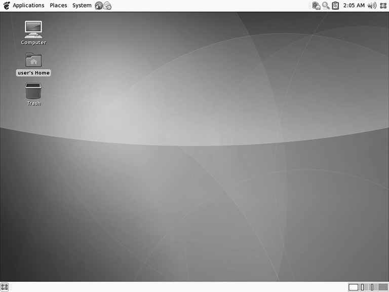
FIGURE 9-1
GNOME.
Courtesy of The GNOME Project
K Desktop Environment (KDE)/Plasma
KDE (http://www.kde.org) is the other of the two most popular Linux GUIs available. Most Linux distributions ship with either KDE or GNOME, or both. For example, the Kbuntu distribution is essentially Ubuntu with KDE. KDE was founded in 1996 by Matthias Ettrich. At the time of KDE’s creation, Ettrich was, like Linus Torvalds, a computer science student. The name KDE was intended as a word play on the Common Desktop Environment (CDE) available for UNIX systems. Today, the K stands for nothing and the acronym stands for K Desktop Environment. KDE is built on the Qt framework. Qt is a multiplatform GUI framework written in C++. KDE is shown in FIGURE 9-2.
Although KDE and GNOME are the most widely known and used graphical user interfaces for Linux, there are certainly others. A couple of the more widely used are listed and briefly described here:
Common Desktop Environment (CDE)—The CDE (http://www.opengroup.org/cde/) was originally developed in 1994 for UNIX systems. At one time it was the default desktop for Sun Solaris systems. CDE is based on HP’s Visual User Environment (VUE).
Enlightenment—This desktop is rather new and is meant specifically for graphics developers. You can learn more at http://www.enlightenment.org.
Linux Boot Process
It is important to understand the Linux boot process because some crimes, including malware attacks, can affect the boot process.
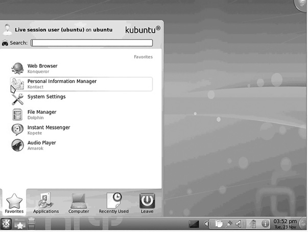
FIGURE 9-2
KDE/Plasma.
Courtesy of KDE.
Linux is often used on embedded systems, even smartphones. In such cases, when the system is first powered on, the first step is to load the bootstrap environment. The bootstrap environment is a special program, such as U-Boot or RedBoot, that is stored in a special section of flash memory. On a PC, booting Linux begins in the BIOS (basic input/output system) at address 0xFFFF0.
Just as with Windows, the first sector on any disk is called the boot sector. It contains executable code that is used in the boot process. A boot sector also has the hex value 0xaa55 in the final 2 bytes. Also, as in Windows, after the BIOS has been loaded and the power-on self test (POST) has completed, the BIOS locates the master boot record (MBR) and passes control to it.
The MBR then loads up a boot loader program, such as LILO (Linux Loader) or GRUB (Grand Unified Bootloader). GRUB is the more modern and much more widely used boot loader. Often boot loaders are larger than a single sector, so they are loaded in stages. When a bootable device is found, the first-stage boot loader is loaded into random access memory (RAM) and executed.
In Linux, there are actually two boot loaders. The first boot loader is rather small, only 512 bytes (a single sector). The first 446 bytes are the primary boot loader, which contains both executable code and error message text. The next 64 bytes are the partition table, which contains a record for each of four partitions. Each is just 16 bytes. The first boot loader is terminated with 2 bytes that are defined as the magic number (0xAA55). This boot loader’s job is to load the second-stage boot loader. The second boot loader is responsible for loading the Linux kernel.
When the second-stage boot loader is loaded into RAM and executing, a splash screen is commonly displayed. At this point, the Linux image is loaded into RAM. When the images are loaded, the second-stage boot loader passes control to the kernel image and the kernel is decompressed and initialized.
At this point, the second-stage boot loader checks the system hardware and any attached peripherals. Once the devices are enumerated, the second-stage boot loader can attempt to mount the root device and load the necessary kernel modules.
The second-stage boot loader loads the kernel image. This is called the kernel stage of the boot process. The kernel must initialize any devices the system has. Even devices that have been initialized by the BIOS must be reinitialized. The system then switches the CPU from real mode to protected mode. The system now loads the compressed kernel and calls the decompress_kernel() function. It is at this point that you may see the “Uncompressing Linux...” message displayed on the screen. Now the start_kernel() function is called, and the uncompressed kernel displays a large number of messages on the screen as it initializes the various hardware items and processes such as the scheduler.
Once the kernel is initialized, the first user program starts. In PC-based Linux systems, that first process is called init, short for initialization. The kernel_thread() function is called next to start init. The kernel goes into an idle loop and becomes an idle thread with process ID 0. The process init() begins high-level system initialization. Note that unlike PC systems, embedded systems have a simpler first user process than init.
The boot process then inspects the /etc/inittab file to determine the appropriate run level. As a reference, the Linux run levels are listed in TABLE 9-2.
Based on the run level, the init process then executes the appropriate start-up script. Those scripts are located in subdirectories of the /etc/rc.d directory. Scripts used for run levels 0 to 6 are located in subdirectories /etc/rc.d/rc0.d through /etc/rc.d/rc6.d, respectively. The default boot run level is set in the file /etc/inittab with the initdefault variable. At this point, the boot process is over, and Linux is up and running!
Logical Volume Manager
Logical Volume Manager (LVM) is an abstraction layer that provides volume management for the Linux kernel. The technology has many purposes, but on a single system (like a single desktop or server) its primary role is to allow the resizing of partitions and the creation of backups by taking snapshots of the logical volumes.
With LVM, the first megabyte of the physical drive or volume (called a PV) contains a structure called the LVM header. The PV for a drive contains that drive or volume’s layout. The Scientific Working Group on Digital Evidence (SWGDE) describes LVM as follows:
|
TABLE 9-2 Typical default active services. |
||
MODE |
DIRECTORY |
RUN LEVEL DESCRIPTION |
0 |
/etc/rc.d/rc0.d |
Halt |
1 |
/etc/rc.d/rc1.d |
Single-user mode |
2 |
/etc/rc.d/rc2.d |
Not used (user-definable) |
3 |
/etc/rc.d/rc3.d |
Full multiuser mode without GUI |
4 |
/etc/rc.d/rc4.d |
Not used (user-definable) |
5 |
/etc/rc.d/rc5.d |
Full multiuser mode with GUI |
6 |
/etc/rc.d/rc6.d |
Reboot |
Some Linux installations use LVM, a logical volume manager for the Linux kernel that manages disk drives and similar mass-storage devices, providing an abstraction layer on top of traditional partitions and block devices. LVM provides a more flexible configuration of storage on block devices by virtualizing the partitions and allowing them to be split, combined, and or arrayed across independent physical disks or physical partitions. In order to parse on-disk structures properly, forensic tools must be LVM aware. Acquisition of an LVM volume must consider the logical configuration of the storage.1
Linux Distributions
Linux is open source. That means the source code is available for anyone who wants to modify, repackage, and distribute it. Therefore, a lot of different distributions are available. They are all Linux, they all have the same Linux shells, but each has some differences. For example, some use KDE by default, whereas others use GNOME. Some ship with lots of additional open source tools, whereas others don’t have quite as many tools, or have different tools. A few of the more common distributions include the following:
Ubuntu—Very popular with beginners
Red Hat Enterprise Linux (RHEL)—Often used with large-scale servers
OpenSuse—A popular, general-purpose Linux distribution
Debian—Another popular, general-purpose Linux distribution
Slackware—Becoming more popular
The website http://www.DistroWatch.com has a list of the 100 best-selling distributions.
At one time, BackTrack was the most interesting distribution to forensic analysts. BackTrack was replete with tools for penetration testing and forensics. As of March 2013, however, support for BackTrack was officially stopped. It is a good idea to become at least familiar with how BackTrack was originally based on the Knoppix distribution but is now based on the Debian distribution and re-released as Kali Linux. Kali Linux is covered in more depth later in the chapter. For more information about working with BackTrack, there are some great tutorials at http://www.backtrack-linux.org/tutorials/.