InfluxDB provides an SQL-like query language; it is used for querying time-series data. It also supports HTTP APIs for write and performs admin-related work.
Let's use the InfluxDB CLI tool to connect to an InfluxDB instance and run some queries.
Start and connect to the InfluxDB instance by typing the following commands:
sudo service InfluxDB start
$ influx -precision rfc3339
By default, InfluxDB shows the time as nanosecond UTC value, it is a very long number, like 1511815800000000000. The argument -precision rfc3339 is for the display time field as a human readable format - YYYY-MM-DDTHH:MM:SS.nnnnnnnnnZ:
Connected to http://localhost:8086 version 1.5
InfluxDB shell version: 1.5
>
We can check available databases by using the show databases function:
> show databases;
name: databases
name
----
_internal
To use the command to switch to an existing database, you can type the following command:
use _internal
This command will switch to the existing database and set your default database to _internal. Doing this means all subsequent commands you write to CLI will automatically be executed on the _internal database until you switch to another database.
So far, we haven't created any new database. At this stage, it shows the default database _internal provided by the product itself. If you want to view all of the available measurements for the current database, you can use the following command:
show measurements
Let's quickly browse the measurements under the _internal database.
> use _internal
Using database _internal
> show measurements
name: measurements
name
----
cq
database
httpd
queryExecutor
runtime
shard
subscriber
tsm1_cache
tsm1_engine
tsm1_filestore
tsm1_wal
write
We can see that the _internal database contains lots of system-level statistical data, which can store very useful system information and help you analyze the system information.
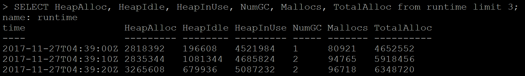
For example, if you want to check heap usage over the time, you can run an SQL-like SELECT statement command to query and get more information:
SELECT HeapAlloc, HeapIdle, HeapInUse, NumGC, Mallocs, TotalAlloc from runtime limit 3;
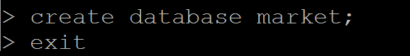
It's time to create our first InfluxDB database! In our sample project, we will use real-time intra day stock quotes market data to set up our lab. The sample data contains November 27, 2017 to November 29, 2017 market stock data for three companies: Apple Inc, JPMorgan Chase & Co., and Alphabet Inc. The interval is 60 seconds.
Here is the example data format:
tickers,ticker=JPM company="JPMorgan Chase & Co",close=98.68,high=98.7,low=98.68,open=98.7,volume=4358 151179804
tickers,ticker=JPM company="JPMorgan Chase & Co",close=98.71,high=98.7,low=98.68,open=98.68,volume=1064 151179810
In the data shown here, we separated measurement, tag set and field set use comma, each tag set and field set are separated by space: measurement, tag set..., field set.... . Define the ticker as tag set and define company, close, high, low, open, volume as fields set. The last value is UTC time. The measurement name is tickers.
Download the sample data to the Unix box:
/tmp/data/ticker_data.txt
Then, load the data to the market database:
/tmp/data$ influx -import -path=/tmp/data/ticker_data.txt -database=market -precision=s
2017/11/30 12:13:17 Processed 1 commands
2017/11/30 12:13:17 Processed 3507 inserts
2017/11/30 12:13:17 Failed 0 inserts
In InfluxDB CLI, verify the new measurement tickers that are created:
> show measurements;
name: measurements
name
----
tickers
The SELECT statement is used to retrieve data points from one or more measurements. The InfluxDB query syntax is as follows:
SELECT <field_key>[,<field_key>,<tag_key>] FROM <measurement_name>[,<measurement_name>] WHERE <conditional_expression> [(AND|OR) <conditional_expression> [...]]
The following are the arguments for SELECT:
|
Name |
Description |
|
SELECT |
This statement is used to fetch data points from one or more measurements |
|
* |
This indicates all tag keys and field keys and the time |
|
field_key |
This returns a specific field |
|
tag_key |
This returns a specific tag |
|
SELECT "<field_key>"::field,"<tag_key>"::tag |
This returns a specific field and tag; the ::[field | tag] syntax specifies the identifier's type |
|
FROM <measurement_name>,<measurement_name> |
This returns data from one or more measurements |
|
FROM <database_name>.<retention_policy_name>.<measurement_name> |
This returns a fully qualified measurement |
|
FROM <database_name>..<measurement_name> |
This returns specific database measurement with default RP |
Let's look at some examples for a better understanding.
The query selects all of the fields, tags, and time from tickers measurements:
> select * from tickers;
name: tickers
time close company high low open ticker volume
---- ----- ------- ---- --- ---- ------ ------
2017-11-27T05:00:00Z 174.05 APPLE INC 174.105 174.05 174.06 AAPL 34908
2017-11-27T05:00:00Z 98.42 JPMorgan Chase & Co 98.44 98.4 98.4 JPM 7904
2017-11-27T05:00:00Z 1065.06 Alphabet Inc 1065.06 1065.06 1065.06 GOOGL 100
[....]
The query selects the field key and tag key from the tickers measurements:
> select ticker, company, close, volume from tickers;
name: tickers
time ticker company close volume
---- ------ ------- ----- ------
2017-11-27T05:00:00Z AAPL APPLE INC 174.05 34908
2017-11-27T05:00:00Z JPM JPMorgan Chase & Co 98.42 7904
2017-11-27T05:00:00Z GOOGL Alphabet Inc 1065.06 100
2017-11-27T05:01:00Z JPM JPMorgan Chase & Co 98.365 20155
[...]
The query selects the field key and tag key based on the identifier type from tickers measurements:
> SELECT ticker::tag,company::field,volume::field,close::field FROM tickers limit 3;
name: tickers
time ticker company volume close
---- ------ ------- ------ -----
2017-11-27T05:00:00Z AAPL APPLE INC 34908 174.05
2017-11-27T05:00:00Z JPM JPMorgan Chase & Co 7904 98.42
2017-11-27T05:00:00Z GOOGL Alphabet Inc 100 1065.06
The query selects all of the fields based on the identifier type from tickers measurements:
> SELECT *::field FROM tickers limit 3;
name: tickers
time close company high low open volume
---- ----- ------- ---- --- ---- ------
2017-11-27T05:00:00Z 174.05 APPLE INC 174.105 174.05 174.06 34908
2017-11-27T05:00:00Z 98.42 JPMorgan Chase & Co 98.44 98.4 98.4 7904
2017-11-27T05:00:00Z 1065.06 Alphabet Inc 1065.06 1065.06 1065.06 100
The query selects fully qualified ticker measurements:
> SELECT ticker, company, volume, close FROM market.autogen.tickers limit 3;
name: tickers
time ticker company volume close
---- ------ ------- ------ -----
2017-11-27T05:00:00Z AAPL APPLE INC 34908 174.05
2017-11-27T05:00:00Z JPM JPMorgan Chase & Co 7904 98.42
2017-11-27T05:00:00Z GOOGL Alphabet Inc 100 1065.06
The following is a list of arguments for WHERE:
|
WHERE supported operators |
Operation |
|
= |
equal to |
|
<> |
not equal to |
|
!= |
not equal to |
|
> |
greater than |
|
>= |
greater than or equal to |
|
< |
less than |
|
<= |
less than or equal to |
|
Tags: tag_key <operator> ['tag_value'] |
Single quote for tag value, since tag value is of string type |
|
timestamps |
The default time range is between 1677-09-21 00:12:43.145224194 and 2262-04-11T23:47:16.854775806Z UTC |
Let's look at some examples of this argument for a better understanding.
The query returns all tickers when high is larger than 174.6 and ticker is AAPL:
> SELECT * FROM tickers WHERE ticker='AAPL' AND high> 174.6 limit 3;
name: tickers
time close company high low open ticker volume
---- ----- ------- ---- --- ---- ------ ------
2017-11-27T14:30:00Z 175.05 APPLE INC 175.06 174.95 175.05 AAPL 261381
2017-11-27T14:31:00Z 174.6 APPLE INC 175.05 174.6 175 AAPL 136420
2017-11-27T14:32:00Z 174.76 APPLE INC 174.77 174.56 174.6003 AAPL 117050
The query performs basic arithmetic to find out the date when the ticker is JPM and high price is more than the low price by 0.2%:
> SELECT * FROM tickers WHERE ticker='JPM' AND high> low* 1.002 limit 5;
name: tickers
time close company high low open ticker volume
---- ----- ------- ---- --- ---- ------ ------
2017-11-27T14:31:00Z 98.14 JPMorgan Chase & Co 98.31 98.09 98.31 JPM 136485
2017-11-27T14:32:00Z 98.38 JPMorgan Chase & Co 98.38 98.11 98.12 JPM 27837
2017-11-27T14:33:00Z 98.59 JPMorgan Chase & Co 98.59 98.34 98.38 JPM 47042
2017-11-27T14:41:00Z 98.89 JPMorgan Chase & Co 98.9 98.68 98.7 JPM 51245
2017-11-29T05:05:00Z 103.24 JPMorgan Chase & Co 103.44 103.22 103.44 JPM 73835
InfulxDB supports group by. The GROUP BY statement is often used with aggregate functions (COUNT, MEAN, MAX, MIN, SUM, AVG) to group the result set by one or more tag keys.
The following is the syntax:
SELECT_clause FROM_clause [WHERE_clause] GROUP BY [* | <tag_key>[,<tag_key]]
The following are the arguments for the GROUP BY TAG_KY:
|
GROUP BY * |
Groups by all tags |
|
GROUP BY <tag_key> |
Groups by a specific tag |
|
GROUP BY <tag_key>,<tag_key> |
Groups by multiple specific tags |
|
Supported Aggregation functions: COUNT(), DISTINCT(), INTEGRAL(), MEAN(), MEDIAN(), MODE(), SPREAD(), STDDEV(), SUM() |
|
|
Supported Selector functions: BOTTOM(), FIRST(), LAST(), MAX(), MIN(), PERCENTILE(), SAMPLE(), TOP() |
Consider the following example:
The query finds all tickers' maximum volumes, minimum volumes, and median volumes during 10-19, November 27, 2017:
> select MAX(volume), MIN(volume), MEDIAN(volume) from tickers where time <= '2017-11-27T19:00:00.000000000Z' AND time >= '2017-11-27T10:00:00.000000000Z' group by ticker;
name: tickers
tags: ticker=AAPL
time max min median
---- --- --- ------
2017-11-27T10:00:00Z 462796 5334 32948
name: tickers
tags: ticker=GOOGL
time max min median
---- --- --- ------
2017-11-27T10:00:00Z 22062 200 1950
name: tickers
tags: ticker=JPM
time max min median
---- --- --- ------
2017-11-27T10:00:00Z 136485 2400 14533
By change group by *, it will group the query result for all tags:
> select MAX(volume), MIN(volume), MEDIAN(volume) from tickers where time <= '2017-11-27T19:00:00.000000000Z' AND time >= '2017-11-27T10:00:00.000000000Z' group by *;
name: tickers
tags: ticker=AAPL
time max min median
---- --- --- ------
2017-11-27T10:00:00Z 462796 5334 32948
name: tickers
tags: ticker=GOOGL
time max min median
---- --- --- ------
2017-11-27T10:00:00Z 22062 200 1950
name: tickers
tags: ticker=JPM
time max min median
---- --- --- ------
2017-11-27T10:00:00Z 136485 2400 14533
InfluxDB supports the arguments for GROUP BY - time interval, the following is the syntax:
SELECT <function>(<field_key>) FROM_clause WHERE <time_range> GROUP BY time(<time_interval>),[tag_key] [fill(<fill_option>)]
|
Syntax |
Descrption |
|
time_range |
Range of timestamp field, time > past time and < future time |
|
time_interval |
Duration literal, group query result into the duration time group |
|
fill(<fill_option>) |
Optional. When time intervals have no data, it can change to fill the value |
Let's look at some examples for a better understanding.
Find stock trade volumes' mean value during 10-19, November 27, 2017, and group the results into 60-minute intervals and ticker tag key:
> select mean(volume) from tickers where time <= '2017-11-27T19:00:00.000000000Z' AND time >= '2017-11-27T10:00:00.000000000Z' group by time(60m), ticker;
name: tickers
tags: ticker=AAPL
time mean
---- ----
2017-11-27T10:00:00Z
2017-11-27T11:00:00Z
2017-11-27T12:00:00Z
2017-11-27T13:00:00Z
2017-11-27T14:00:00Z 139443.46666666667
2017-11-27T15:00:00Z 38968.916666666664
2017-11-27T16:00:00Z 44737.816666666666
2017-11-27T17:00:00Z
2017-11-27T18:00:00Z 16202.15
2017-11-27T19:00:00Z 12651
name: tickers
tags: ticker=GOOGL
time mean
---- ----
2017-11-27T10:00:00Z
2017-11-27T11:00:00Z
2017-11-27T12:00:00Z
2017-11-27T13:00:00Z
2017-11-27T14:00:00Z 6159.033333333334
2017-11-27T15:00:00Z 2486.75
2017-11-27T16:00:00Z 2855.5
2017-11-27T17:00:00Z
2017-11-27T18:00:00Z 1954.1166666666666
2017-11-27T19:00:00Z 300
name: tickers
tags: ticker=JPM
time mean
---- ----
2017-11-27T10:00:00Z
2017-11-27T11:00:00Z
2017-11-27T12:00:00Z
2017-11-27T13:00:00Z
2017-11-27T14:00:00Z 35901.8275862069
2017-11-27T15:00:00Z 17653.45
2017-11-27T16:00:00Z 14139.25
2017-11-27T17:00:00Z
2017-11-27T18:00:00Z 14419.416666666666
2017-11-27T19:00:00Z 4658
InfluxDB supports the INTO clause. You can copy from one measurement to another or create a new database for measurement.
The following is the syntax:
SELECT_clause INTO <measurement_name> FROM_clause [WHERE_clause] [GROUP_BY_clause]
|
Syntax |
Description |
|
INTO <measurement_name> |
This helps you to copy data into a specific measurement. |
|
INTO <database_name>.<retention_policy_name>.<measurement_name> |
This helps you to copy data into a fully qualified measurement. |
|
INTO <database_name>..<measurement_name> |
This helps you to copy data into a specified measurement with a default RP. |
|
INTO <database_name>.<retention_policy_name>.:MEASUREMENT FROM /<regular_expression>/ |
This helps you to copy data into a specified database with RP and using regular expression match from the clause. |
Let's take a look at some examples for a better understanding.
Copy the aggregate mean of all of the field values into a different database and create a new measurement:
> use market
Using database market
> SELECT MEAN(*) INTO market_watch.autogen.avgvol FROM /.*/ WHERE time >= '2017-11-27T00:00:00.000000000Z' AND time <= '2017-11-27T23:59:59.000000000Z' GROUP BY time(60m);
name: result
time written
---- -------
1970-01-01T00:00:00Z 8
> use market_watch
Using database market_watch
> show measurements;
name: measurements
name
----
avgvol
tickers
> select * from avgvol
name: avgvol
time mean_close mean_high mean_low mean_open mean_volume
---- ---------- --------- -------- --------- -----------
2017-11-27T05:00:00Z 435.3618644067796 435.43688926553676 435.27535762711864 435.33908870056507 16300.42372881356
2017-11-27T14:00:00Z 448.45324269662916 448.67904269662927 448.16110786516856 448.42909325842686 60777.84269662921
2017-11-27T15:00:00Z 446.46472277777775 446.5794283333334 446.3297522222223 446.4371933333333 19703.03888888889
2017-11-27T16:00:00Z 445.9267622222222 446.0731233333333 445.7768644444446 445.9326772222222 20577.522222222222
2017-11-27T18:00:00Z 447.22421222222226 447.29334333333327 447.1268016666667 447.1964166666667 10858.56111111111
2017-11-27T19:00:00Z 440.0175634831461 440.1042516853933 439.9326162921348 440.02026348314615 11902.247191011236
2017-11-27T20:00:00Z 447.3597166666667 447.43757277777786 447.2645472222222 447.3431649999999 19842.32222222222
2017-11-27T21:00:00Z 448.01033333333334 448.43833333333333 448.00333333333333 448.29333333333335 764348.3333333334