The preceding figure showed that write is stored both in memory and on disk. Periodically, the data is flushed from memory to disk:

Additionally, deletes in Cassandra are written to disk in structures known as tombstones. A tombstone is essentially a timestamped placeholder for a delete. The tombstone gets replicated out to all of the other nodes responsible for the deleted data. This way, reads for that key will return consistent results, and prevent the problems associated with ghost data.

Eventually, SSTable files are merged together and tombstones are reclaimed in a process called compaction. While it takes a while to run, compaction is actually a good thing and ultimately helps to increase (mostly read) performance by reducing the number of files (and ultimately disk I/O) that need to be searched for a query. Different compaction strategies can be selected based on the use case. While it does impact performance, compaction throughput can be throttled (manually), so that it does not affect the node's ability to handle operations.

In a distributed database environment (especially one that spans geographic regions), it is entirely possible that write operations may occasionally fail to distribute the required amount of replicas. Because of this, Cassandra comes with a tool known as repair. Cassandra anti-entropy repairs have two distinct operations:

• Merkle trees are calculated for the current node (while communicating with other nodes) to determine replicas that need to be repaired (replicas that should exist, but do not)
• Data is streamed from nodes that contain the desired replicas to fix the damaged replicas on the current node

To maintain data consistency, repair of the primary token ranges must be run on each node within the gc_grace_seconds period (default is 10 days) for a table. The recommended practice is for repairs to be run on a weekly basis.

Read operations in Cassandra are slightly more complex in nature. Similar to writes, they are served by structures that reside both on disk and in memory:

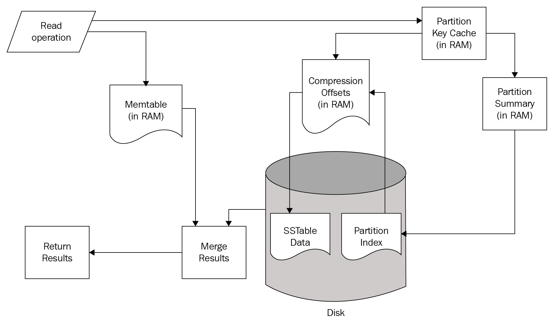
A Read operation simultaneously checks structures in memory and on Disk. If the requested data is found in the Memtable structures of the current node, that data is merged with results obtained from the disk.

The read path from the disk also begins in memory. First, the Bloom Filter is checked. The Bloom Filter is a probability-based structure that speeds up reads from disk by determining which SSTables are likely to contain the requested data.

If the Bloom Filter was unable to determine which SSTables to check, the Partition Key Cache is queried next. The key cache is enabled by default, and uses a small, configurable amount of RAM.^[6] If a partition key is located, the request is immediately routed to the Compression Offset.

If a partition key is not located in the Partition Key Cache, the Partition Summary is checked next. The Partition Summary contains a sampling of the partition index data, which helps determine a range of partitions for the desired key. This is then verified against the Partition Index, which is an on-disk structure containing all of the partition keys.

Once a seek is performed against the Partition Index, its results are then passed to the Compression Offset. The Compression Offset is a map structure which^[6] stores the on-disk locations for all partitions. From here, the SSTable containing the requested data is queried, the data is then merged with the Memtable results, and the result set is built and returned.

One important takeaway, from analyzing the Cassandra read path, is that queries that return nothing do consume resources. Consider the possible points where data stored in Cassandra may be found and returned. Use of several of the structures in the read path only happens if the requested data is not found in the prior structure. Therefore, using Cassandra to check for the mere existence of data is not an efficient use case.