We have been talking about using the recall metric as our proxy for how effective our predictive model is. Even though recall is still the recall we want to calculate, bear mind in mind that the under-sampled data isn't skewed toward a certain class, which doesn't make the recall metric as critical.

We use this parameter to build the final model with the whole training dataset and predict the classes in the test data:

# dataset
lr = LogisticRegression(C = best_c, penalty = 'l1')
lr.fit(X_train_undersample,y_train_undersample.values.ravel())
y_pred_undersample = lr.predict(X_test_undersample.values)

Here is the compute confusion matrix:

cnf_matrix = confusion_matrix(y_test_undersample,y_pred_undersample)
np.set_printoptions(precision=2)

print("Recall metric in the testing dataset: ", cnf_matrix[1,1]/(cnf_matrix[1,0]+cnf_matrix[1,1]))

We plot the non-normalized confusion matrix as follows:

class_names = [0,1]
plt.figure()
plot_confusion_matrix(cnf_matrix, classes=class_names, title='Confusion matrix')
plt.show()

Here is the output for the preceding code:

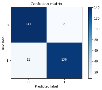
Hence, the model is offering a 92.5% recall accuracy on the generalized unseen data (test set), which is not a bad percentage on the first try. However, keep in mind that this is a 92.5% recall accuracy measure on the under-sampled test set. We will apply the model we fitted and test it on the whole data, as shown:

We Use this parameter to build the final model with the whole training dataset and predict the classes in the test
# dataset
lr = LogisticRegression(C = best_c, penalty = 'l1')
lr.fit(X_train_undersample,y_train_undersample.values.ravel())
y_pred = lr.predict(X_test.values)

# Compute confusion matrix
cnf_matrix = confusion_matrix(y_test,y_pred)
np.set_printoptions(precision=2)

print("Recall metric in the testing dataset: ", cnf_matrix[1,1]/(cnf_matrix[1,0]+cnf_matrix[1,1]))

# Plot non-normalized confusion matrix
class_names = [0,1]
plt.figure()
plot_confusion_matrix(cnf_matrix, classes=class_names, title='Confusion matrix')
plt.show()

Here is the output from the preceding code:

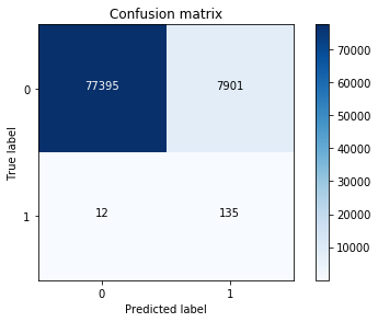
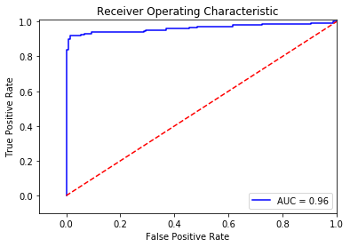
We still have a very decent recall accuracy when applying it to a much larger and skewed dataset. By plotting ROC curve and precision-recall curve, we find that the precision-recall curve is much more convenient as our problems relies on the positive class being more interesting than the negative class, but, as we have calculated the recall precision, we will not plot the precision-recall curves. AUC and ROC curves are also interesting to check whether the model is also predicting as a whole correctly and not making many errors:

# ROC CURVE
lr = LogisticRegression(C = best_c, penalty = 'l1')
y_pred_undersample_score = lr.fit(X_train_undersample,y_train_undersample.values.ravel()).decision_function(X_test_undersample.values)
fpr, tpr, thresholds = roc_curve(y_test_undersample.values.ravel(),y_pred_undersample_score)
roc_auc = auc(fpr,tpr)
# Plot ROC
plt.title('Receiver Operating Characteristic')
plt.plot(fpr, tpr, 'b',label='AUC = %0.2f'% roc_auc)
plt.legend(loc='lower right')
plt.plot([0,1],[0,1],'r--')
plt.xlim([-0.1,1.0])
plt.ylim([-0.1,1.01])
plt.ylabel('True Positive Rate')
plt.xlabel('False Positive Rate')
plt.show()

We get the following output:

An additional process that would be interesting would be to initialize multiple under-sampled datasets and repeat the process in a loop. Remember: to create an under-sampled dataset, we randomly get records from the majority class. Even though this is a valid technique, it doesn't represent the real population, so it would be interesting to repeat the process with different under-sampled configurations and check whether the previous chosen parameters are still the most effective. In the end, the idea is to use a wider random representation of the whole dataset and rely on the averaged best parameters.