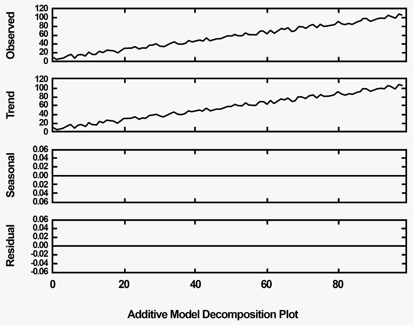
These are random increases or decreases of values in the series. We will be generally dealing with the preceding systematic components in the form of additive models, where additive models can be defined as the sum of level, trend, seasonality, and noise. The other type is called the multiplicative model, where the components are products of each other.

The following graphs help to distinguish between additive and multiplicative models. This graph shows the additive model:

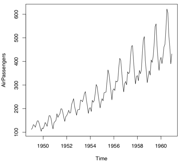
Since data decomposition has a major role in data analyzing, we understand these different components by using pandas inbuilt dataset that is the "International airline passengers: monthly totals in thousands, Jan 49 – Dec 60" dataset. The dataset contains a total of 144 observations of sales from the period of 1949 to 1960 for Box and Jenkins.

Let's import and plot the data:

from pandas import Series
from matplotlib import pyplot
airline = Series.from_csv('/path/to/file/airline_data.csv', header=0)
airline.plot()
pyplot.show()

The following graph shows how there is a seasonality in data and a subsequent increase in the height(amplitude) of the graph as the years have progressed:

We can mathematically compute the trend and the seasonality for the preceding graph with an additive model as shown:

from pandas import Series
from matplotlib import pyplot
from statsmodels.tsa.seasonal import seasonal_decompose
airline = Series.from_csv('/path/to/file/airline_data.csv', header=0)
result = seasonal_decompose(airline, model='additive')
result.plot()
pyplot.show()

The output for the preceding code is as shown follows:

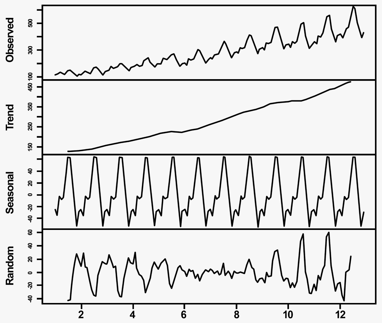
The preceding graph can be interpreted as follows:

• Observed: The regular airline data graph
• Trend: The observed increase in trend
• Seasonality: The observed seasonality in the data
• Random: This is first observed graph after removing the initial seasonal patterns