We will revisit a problem that is detecting malicious URLs, and we will find a way to solve the same with decision trees. We start by loading the data:

 from urlparse import urlparse
 import pandas as pd
 urls = pd.read_json("../data/urls.json")
 print urls.shape
 urls['string'] = "http://" + urls['string']

(5000, 3)

On printing the head of the urls:

urls.head(10)

The output looks as follows:

Following code is used to produce the output in formats of truth and string from the dataset:

X, y = urls['truth'], urls['string']
X.head()  # look at X

On executing previous code you will have the following output:

 0    http://startbuyingstocks.com/
 1                http://qqcvk.com/
 2        http://432parkavenue.com/
 3           http://gamefoliant.ru/
 4                  http://orka.cn/
 Name: string, dtype: object

We get our null accuracy because we are interested in prediction where 0 is not malicious:

y.value_counts(normalize=True)


 0    0.9694
 1    0.0306
 Name: truth, dtype: float64

We create a function called custom_tokenizer that takes in a string and outputs a list of tokens of the string:

from sklearn.feature_extraction.text import CountVectorizer
 import re
 
 def custom_tokenizer(string):
    final = []
    tokens = [a for a in list(urlparse(string)) if a]
    for t in tokens:
        final.extend(re.compile("[.-]").split(t))
    return final

print custom_tokenizer('google.com')
 
 print custom_tokenizer('https://google-so-not-fake.com?fake=False&seriously=True')

['google', 'com']
['https', 'google', 'so', 'not', 'fake', 'com', 'fake=False&seriously=True']

We first use logistic regression . The relevant packages are imported as follows:

from sklearn.pipeline import Pipeline
 from sklearn.linear_model import LogisticRegression
vect = CountVectorizer(tokenizer=custom_tokenizer)
 lr = LogisticRegression()
 lr_pipe = Pipeline([('vect', vect), ('model', lr)])

from sklearn.model_selection import cross_val_score, GridSearchCV, train_test_split
scores = cross_val_score(lr_pipe, X, y, cv=5)
scores.mean()  # not good enough!!

The output can be seen as follows:

0.980002384002384

We will be using random forest to detect malicious urls. The theory of random forest will be discussed in the next chapter on decision trees. To import the pipeline, we get the following:

from sklearn.pipeline import Pipeline
 from sklearn.ensemble import RandomForestClassifier
 
 rf_pipe = Pipeline([('vect', vect), ('model',  RandomForestClassifier(n_estimators=500))])
 scores = cross_val_score(rf_pipe, X, y, cv=5)
 
 scores.mean()  # not as good

The output can be seen as follows:

0.981002585002585

We will be creating the test and train datasets and then creating the confusion matrix for this as follows:

X_train, X_test, y_train, y_test = train_test_split(X, y)
from sklearn.metrics import confusion_matrix
rf_pipe.fit(X_train, y_train)
preds = rf_pipe.predict(X_test)
 print confusion_matrix(y_test, preds)  # hmmmm

[[1205    0]
 [  27 18]]

We get the predicted probabilities of malicious data:

probs = rf_pipe.predict_proba(X_test)[:,1]  

We play with the threshold to alter the false positive/negative rate:

import numpy as np  
 for thresh in [.1, .2, .3, .4, .5, .6, .7, .8, .9]:
    preds = np.where(probs >= thresh, 1, 0)
    print thresh
    print confusion_matrix(y_test, preds)
    print

The output looks as follows:

0.1
 [[1190   15]
 [  15 30]]
 
 0.2
 [[1201    4]
 [  17 28]]
 
 0.3
 [[1204    1]
 [  22 23]]
 
 0.4
 [[1205    0]
 [  25 20]]
 
 0.5
 [[1205    0]
 [  27 18]]
 
 0.6
 [[1205    0]
 [  28 17]]
 
 0.7
 [[1205    0]
 [  29 16]]
 
 0.8
 [[1205    0]
 [  29 16]]
 
 0.9
 [[1205    0]
 [  30 15]]

We dump the importance metric to detect the importance of each of the urls:

pd.DataFrame({'feature':rf_pipe.steps[0][1].get_feature_names(), 'importance':rf_pipe.steps[-1][1].feature_importances_}).sort_values('importance', ascending=False).head(10)

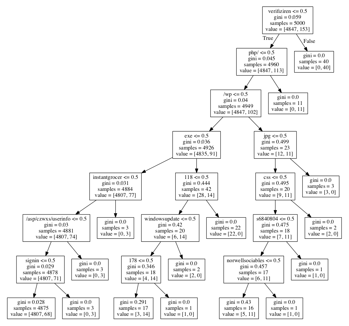
We will use the decision tree classifier as follows:

treeclf = DecisionTreeClassifier(max_depth=7)
 
tree_pipe = Pipeline([('vect', vect), ('model', treeclf)])
 
 vect = CountVectorizer(tokenizer=custom_tokenizer)
 
 scores = cross_val_score(tree_pipe, X, y, scoring='accuracy', cv=5)
 
 print np.mean(scores)
 
 tree_pipe.fit(X, y)
 
 export_graphviz(tree_pipe.steps[1][1], out_file='tree_urls.dot', feature_names=tree_pipe.steps[0][1].get_feature_names())

The level of accuracy is 0.98:

0.9822017858017859

The tree diagram below shows how the decision logic for maliciousness detection works.