Table of Contents for
Web Mapping Illustrated
 Web Mapping Illustrated
Published by
O'Reilly Media, Inc., 2005
Web Mapping Illustrated
Published by
O'Reilly Media, Inc., 2005
- Web Mapping Illustrated
- Cover
- Web Mapping Illustrated
- A Note Regarding Supplemental Files
- Foreword
- Preface
- Youthful Exploration
- The Tools in This Book
- What This Book Covers
- Organization of This Book
- Conventions Used in This Book
- Safari Enabled
- Comments and Questions
- Acknowledgments
- 1. Introduction to Digital Mapping
- 1.1. The Power of Digital Maps
- 1.2. The Difficulties of Making Maps
- 1.3. Different Kinds of Web Mapping
- 2. Digital Mapping Tasks and Tools
- 2.1. Common Mapping Tasks
- 2.2. Common Pitfalls, Deadends, and Irritations
- 2.3. Identifying the Types of Tasks for a Project
- 3. Converting and Viewing Maps
- 3.1. Raster and Vector
- 3.2. OpenEV
- 3.3. MapServer
- 3.4. Geospatial Data Abstraction Library (GDAL)
- 3.5. OGR Simple Features Library
- 3.6. PostGIS
- 3.7. Summary of Applications
- 4. Installing MapServer
- 4.1. How MapServer Applications Operate
- 4.2. Walkthrough of the Main Components
- 4.3. Installing MapServer
- 4.4. Getting Help
- 5. Acquiring Map Data
- 5.1. Appraising Your Data Needs
- 5.2. Acquiring the Data You Need
- 6. Analyzing Map Data
- 6.1. Downloading the Demonstration Data
- 6.2. Installing Data Management Tools: GDAL and FWTools
- 6.3. Examining Data Content
- 6.4. Summarizing Information Using Other Tools
- 7. Converting Map Data
- 7.1. Converting Map Data
- 7.2. Converting Vector Data
- 7.3. Converting Raster Data to Other Formats
- 8. Visualizing Mapping Data in a Desktop Program
- 8.1. Visualization and Mapping Programs
- 8.2. Using OpenEV
- 8.3. OpenEV Basics
- 9. Create and Edit Personal Map Data
- 9.1. Planning Your Map
- 9.2. Preprocessing Data Examples
- 10. Creating Static Maps
- 10.1. MapServer Utilities
- 10.2. Sample Uses of the Command-Line Utilities
- 10.3. Setting Output Image Formats
- 11. Publishing Interactive Maps on the Web
- 11.1. Preparing and Testing MapServer
- 11.2. Create a Custom Application for a Particular Area
- 11.3. Continuing Education
- 12. Accessing Maps Through Web Services
- 12.1. Web Services for Mapping
- 12.2. What Do Web Services for Mapping Do?
- 12.3. Using MapServer with Web Services
- 12.4. Reference Map Files
- 13. Managing a Spatial Database
- 13.1. Introducing PostGIS
- 13.2. What Is a Spatial Database?
- 13.3. Downloading PostGIS Install Packages and Binaries
- 13.4. Compiling from Source Code
- 13.5. Steps for Setting Up PostGIS
- 13.6. Creating a Spatial Database
- 13.7. Load Data into the Database
- 13.8. Spatial Data Queries
- 13.9. Accessing Spatial Data from PostGIS in Other Applications
- 14. Custom Programming with MapServer’s MapScript
- 14.1. Introducing MapScript
- 14.2. Getting MapScript
- 14.3. MapScript Objects
- 14.4. MapScript Examples
- 14.5. Other Resources
- 14.6. Parallel MapScript Translations
- A. A Brief Introduction to Map Projections
- A.1. The Third Spheroid from the Sun
- A.2. Using Map Projections with MapServer
- A.3. Map Projection Examples
- A.4. Using Projections with Other Applications
- A.5. References
- B. MapServer Reference Guide for Vector Data Access
- B.1. Vector Data
- B.2. Data Format Guide
- ESRI Shapefiles (SHP)
- PostGIS/PostgreSQL Database
- MapInfo Files (TAB/MID/MIF)
- Oracle Spatial Database
- Web Feature Service (WFS)
- Geography Markup Language Files (GML)
- VirtualSpatialData (ODBC/OVF)
- TIGER/Line Files
- ESRI ArcInfo Coverage Files
- ESRI ArcSDE Database (SDE)
- Microstation Design Files (DGN)
- IHO S-57 Files
- Spatial Data Transfer Standard Files (SDTS)
- Inline MapServer Features
- National Transfer Format Files (NTF)
- About the Author
- Colophon
- Copyright
Accessing Spatial Data from PostGIS in Other Applications
Visualizing results isn’t always the end goal of a spatial query. Often, someone just needs to write a report or provide a statistic. However, figures often help explain the data in a way that a report can’t, which is why mapping is such a useful tool for communication.
If you want to visualize the results of PostGIS queries, you have a few options. Depending on what software you use, the simplest method may be to export the data from PostGIS to another format, such as a GML file or an ESRI shapefile. Or you may want to view the data directly in a desktop viewer such as OpenEV or put it in a MapServer web map application.
Exporting PostGIS Data into a Shapefile or GML
You can use the ogr2ogr
utility to convert from PostGIS into many other formats. As discussed
in Chapter 7, it is run from
the command line. Here is an example of how to convert the mycounties view from PostGIS into a
shapefile, though any OGR-supported output format can be used:
> ogr2ogr -f "ESRI Shapefile" mycounties.shp "PG:dbname=project1" mycountiesThe -f parameter specifies
what the output data format will be. The output dataset name will be
mycounties.shp. The source dataset
is the project1 database. The final
word, mycounties, is the name of
the layer to request from PostGIS. In this case it is a PostgreSQL
view, but it can also be a table.
The shapefile can then be loaded into any GIS or mapping product that supports shapefiles. This format is fairly universal. To create a GML file, it looks almost the same:
> ogr2ogr -f "GML" mycounties.gml "PG:dbname=project1" mycountiesAs noted earlier in the "Load Data into the Database"
section, the shp2pgsql and pgsql2shp command-line tools may also be
used. Both shapefiles and GML can be used as a data source for a layer
in MapServer as discussed in Chapters 10 and 11.
Viewing PostGIS Data in OpenEV
The real power of PostGIS is that the data it holds can be accessed directly by a number of applications. When you export data from PostGIS into another format, it is possible for your data to become out of sync. If you can access the data directly from PostGIS, you won’t need to do the exporting step. This has the added benefit of always being able to access the most current data. OpenEV and MapServer are two examples of programs that access PostGIS data directly.
OpenEV can load spatial data from a PostGIS database. This is
only possible if you launch OpenEV from the command line and specify
the database connection you want to access. For example, to access the
project1 database, the command line
to start OpenEV looks like this:
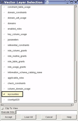
> openev "PG:dbname=project1 user=tyler host=localhost"You will see a long list of warning and status messages as
OpenEV starts up. If it connects to the database properly, you will
see a list of the tables to choose from. Figure 13-5 shows the layer
list from my project1
database.
Warning
The vertical scrollbar seems to have some problems. You may need to resize the window by stretching it taller, to be able to scroll down to find your layers. More recent layers/tables are listed at the bottom.
When you find the layer you want from the list, click on the check mark beside the layer name. The check mark will become darker. Then press the Accept button to load the data into the OpenEV view. The layer is read-only, and changes aren’t saved back into the database.
Viewing PostGIS Data in MapServer
PostGIS is used by many as a data source for MapServer applications. Data management is handled in PostGIS, and MapServer is used as a visualization engine. This combination allows each product to do what it does best.
Appendix B includes examples that use various types of data with MapServer, including PostGIS data. Chapters 10 and 11 describe how to build MapServer applications. The global map example used there can be extended to include a layer of the counties of the United States, based on the examples used earlier in this chapter. The layer can be treated like most other layers but with a few more parameters to help MapServer connect to the database.
Basic MapServer layers, like shapefiles, specify the name of the
source data using the DATA
keyword:
DATA<path to source file>
A PostGIS data source isn’t accessed through a file. Instead, you specify three pieces of database connection information:
CONNECTIONTYPEPOSTGISCONNECTION"dbname=<databasename>host=<host computer name>user=<database user name>port=<default is 5432>"DATA"<geometry column name> from<source data table>"
CONNECTIONTYPE tells
MapServer what kind of data source it is going to load. The CONNECTION parameter is often called the
connection string . It includes the same kind of PostgreSQL connection
information used earlier in this chapter. Some of the information is
optional, but it is a good habit to include all of it even if it is
redundant. Port 5432 is the default port for PostgreSQL. Many problems
new users run into are related to not having enough information
specified here.
Warning
The keyword from used in
the DATA parameter may cause you
grief if it isn’t written in lowercase. It is a known bug that gives
you errors if you use FROM in
uppercase. This bug may be fixed in more recent versions of
MapServer.
Example 13-7 shows the full listing of a layer in the MapServer configuration file, based on the county data loaded into PostGIS earlier on.
LAYER NAMEusa_countiesTYPE POLYGON STATUS DEFAULTCONNECTIONTYPE POSTGIS CONNECTION "dbname=project1 user=tyler host=localhost port=5432" DATA "wkb_geometry from countyp020"CLASS SYMBOL 'circle' SIZE 2 OUTLINECOLOR 0 0 0 END PROJECTION "init=epsg:4326" END END
This example assumes that you have a SYMBOLSET defined with a symbol named
circle available. If you don’t, you
can ignore the SYMBOL'circle' line, but your resulting map will
look slightly different.
The layer in this example is part of a larger map file called
global.map , which also includes some global images showing
elevation changes. To test the map file, use the shp2img command-line utility from your
MapServer installation.
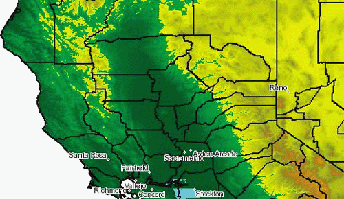
> shp2img -e -122.818 37.815 -121.406 41.003 -m global.map -o fig13-6.pngSee Chapter 10 for more information and some examples using this command. This example draws the layers in the map file, with a focus on a geographic extent covering part of the western United States. The resulting map is saved to an image file called fig13-6.png and is shown in Figure 13-6.
This map includes a few city names from a shapefile and an elevation backdrop from some image files. The county boundary layer (black outlines) is from the PostGIS database. Being able to integrate different types of data into one map is an essential part of many MapServer applications.
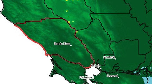
Highlighting a subset of shapes
With some minor modifications to Example 13-7, you can start
to do some basic colortheming. Example 13-8 shows how to
make one county stand out among the others using multiple CLASS objects in the layer, along with the
EXPRESSION parameter. The
resulting map is shown in Figure 13-7.
Tip
For more information about EXPRESSION syntax, see Table 10-1.
LAYER
  NAME usa_counties
  TYPE POLYGON
  STATUS DEFAULT
  CONNECTIONTYPE POSTGIS
  CONNECTION "dbname=project1 user=tyler host=localhost port=5432"
  DATA "wkb_geometry from countyp020"
  CLASS
                     EXPRESSION ("[county]" = 'Sonoma County')
    SYMBOL 'circle'
    SIZE 4
    OUTLINECOLOR 255 0 0
  END
    CLASS
    EXPRESSION ("[county]" != 'Sonoma County')
    SYMBOL 'circle'
    SIZE 2
    OUTLINECOLOR 0 0 0
  END
  PROJECTION
    "init=epsg:4326"
  END
END
Using subqueries for more complex SQL
More sophisticated queries can be used in the DATA line for the layer, but some care is
needed to make it work. For example, if you are more comfortable
with SQL and want to show only Sonoma County, you might be tempted
to use:
DATA "wkb_geometry from countyp020 where county = 'Sonoma County'"
This won’t work. You need to handle any deviation from the
most basic DATA parameter as a
subquery. Here is an example of a subquery, put onto separate lines
for readability only:
DATA "wkb_geometry from(select wkb_geometryfrom countyp020where county = 'Sonoma County')as myquery"
The subquery is the part in the parentheses and can be much
more complex than this example. The myquery keyword is arbitrary but
necessary. It can be any name and is simply a placeholder. MapServer
needs two more pieces of information to handle subqueries. It needs
to be able to uniquely identify each record coming from PostGIS. To
do this, add a using unique
<field
name> clause. If you include a unique
number field in your query use that field name: using unique
countyID. Otherwise you might try using
the geometry field because it will probably have unique values for
every record: using unique
wkb_geometry. It may be not be the most
efficient choice, but it does work.
MapServer also needs to know what spatial reference system the
data will be in. This is specified by adding a using srid =
<
SRID #
> clause. If you already have
a PROJECTION section for your
layer in the map file, you can probably get away with: using srid =
-1, which effectively ignores the
projection settings.
A working example of this subquery method is shown in Example 13-9.
DATA "wkb_geometry from ( select wkb_geometry from countyp020 where
           county = 'Sonoma County') as myquery using unique wkb_geometry
using srid = -1"
A mixture of other PostGIS and PostgreSQL functions can be used in a subquery. For example:
DATA "wkb_geometry from ( select wkb_geometry from countyp020 where
wkb_geometry && 'POINT(-122.88 38.52)' ) as myquery using unique
wkb_geometry using srid = -1"
This example uses the PostGIS bounding box comparison operator
(&&) and a manually
constructed point geometry. It selects the geometry of the county
polygon using the location of the point, just like in earlier
examples in the "Querying
for Spatial Proximity" section.
PostGIS can also create new spatial features through queries,
and MapServer can then map them. For example, you can use the
buffer() function to create a
buffered area around your shape. You can create another layer using
the exact syntax as Example
13-9, but then change it so that it uses a buffer() to expand the shape. It may also
be helpful to simplify the shape a bit so that the buffer is
smoother. Here is a complex example that uses both the buffer() and simplify() functions:
DATA "wkb_geometry from (
select buffer( simplify(wkb_geometry,0.01), 0.2)
         as wkb_geometry
from countyp020
where county='Sonoma County ') as foo
using unique wkb_geometry"
Both functions require a numeric value as well as a geometry
field. These numeric values are always specified in the units of
measure for the coordinates in the data. simplify() weeds out certain vertices
based on a tolerance you provide. In this case it simplifies to a
tolerance of 0.2 degrees. That
simplified shape is then passed to the buffer() function. The buffer drawn around
the features is created 0.01
degrees wide.
Many different types of queries can be used, including queries
from tables, views, or manually constructed geometries in an SQL
statement. For anything other than the most simple table query, be
sure to use the using unique and using srid keywords properly and ensure that the
query returns a valid geometry.
Using PostGIS attributes to draw labels
As with any MapServer data source that has attribute data, PostGIS layers can also use this information to label a map. Example 13-10 is the same as Example 13-8, but includes parameters required for labeling.
LAYER NAME usa_counties TYPE POLYGON STATUS DEFAULT CONNECTIONTYPE POSTGIS CONNECTION "dbname=project1 user=tyler host=localhost port=5432" DATA "wkb_geometry from countyp020"LABELITEM"county"CLASS EXPRESSION ("[county]" = 'Sonoma County') SYMBOL 'circle' SIZE 2 OUTLINECOLOR 0 0 0 #222 120 120LABELCOLOR 0 0 0OUTLINECOLOR 255 255 255TYPE TRUETYPEFONT ARIALSIZE 14ENDEND PROJECTION "init=epsg:4326" END END
This example assumes you have a FONTSET specified in the map file, with a
font named ARIAL available. If
you don’t have these, remove the TYPE, FONT, and SIZE lines in the example.
Adding labels to maps is discussed in more detail in Chapters 10 and 11. With PostGIS, there are a
couple additional considerations to keep in mind. The attribute
specified by LABELITEM must exist
in the table that holds the geometry or in the subquery used. While
this sounds like common sense, it is easy to forget. Example 13-10 has a simple
DATA parameter and doesn’t
include a subquery. Because it points to an existing table, all the
attributes of that table are available to be used as a LABELITEM. However, if a subquery is used
as in Example 13-9,
the attribute used in LABELITEM
must also be returned as part of the subquery. To use the code in
Example 13-9, more
than just the wkb_geometry column
needs to be returned by the subquery. The resulting settings needs
to look like:
DATA "wkb_geometry from ( selectcounty,wkb_geometry from countyp020 where county = 'Sonoma County') as myquery using unique wkb_geometry using srid = -1"
The only addition was county in the subquery. This makes the
county attribute available to
MapServer for use with labels, in addition to the wkb_geometry attribute which was already
part of the subquery.
The other common issue encountered when creating labels is
related to the case of field names. In PostgreSQL (as with other
relational databases), it is possible to have upper- and lowercase
field names, in addition to normal names with no explicit case. All
the field names used in the examples so far have been normal, but
some tools may create fields that are all uppercase, all lowercase,
or (even worse) mixed case. This makes it difficult to refer to
field names because the exact case of every letter in the field name
needs to be specified throughout your MapServer layer parameters.
This is done by using double quotes around field names, which gets
confusing when you may already be using double quotes around a field
name as in LABELITEM "county" in Example 13-10. If the
county attribute is stored as an
uppercase field name, then a set of single quotes must be wrapped
around the field name. The field name must be written in uppercase,
like: LABELITEM
'"COUNTY"'.
Warning
Using attributes for labeling maps is common, but the two
issues related here apply equally to any aspect of the LAYER parameters that refer to PostGIS
fields, not just for labeling purposes, for example in the
DATA, CLASSITEM, and EXPRESSION parameters, and more.
If you use ogr2ogr for
loading data into PostgreSQL, you may need to use another option to
ignore uppercase table and field names. The layer creation option
-lco LAUNDER=YES ensures that all table and
field names are in normal case. By default, ogr2ogr maintains the case used in the
data source.
Using PostGIS in Other Applications
Other open source applications that aren’t discussed in this book, but are able to access PostGIS data, include Quantum GIS (QGIS), uDIG, Java Unified Mapping Platform (JUMP), Thuban, GeoServer, GRASS GIS, etc. Links to these applications are provided in Chapter 8.
Some commercial vendors have implemented PostGIS support as well. Safe Software’s Feature Manipulation Engine supports reading and writing of PostGIS datasets. This powerful tool makes migrating to PostGIS simple and large-scale conversion projects easy. It supports the conversion of dozens of vector and database formats. See http://safe.com for more on licensing and using FME.
Cadcorp’s Spatial Information System (SIS) also supports PostGIS, starting at SIS v6.1. For more information, see their press release at http://www.cadcorp.com.
ArcMap and PostGIS
Even if you’re using PostGIS, your organization may still be using ESRI’s proprietary tools. A common question for ESRI ArcGIS users is “How can I access PostGIS data in ArcMap?” There is an open source project called the PostGIS-ArcMap Connector, PgArc for short. You can find this project at http://pgarc.sourceforge.net/.
PgArc automates the import of PostGIS tables into temporary shapefiles and loads them into ArcMap. Layers can then be edited and put back into PostGIS, overwriting the existing table in the database. There have been some changes introduced with ArcMap 9 that are currently being addressed. More improvements can still be made to strengthen the product; volunteer ArcMap programmers are always welcome.
Another way to access PostGIS data is to use the Web Mapping Server capabilities of MapServer. MapServer can access PostGIS data and create map images using the WMS standard. ESRI has an interoperability extension for ArcMap that allows users to access WMS layers. MapServer is excellent at filling this middle-man role. Chapter 12 is devoted to using MapServer with Open Geospatial Consortium Web Mapping Standards.
For ArcView 3 users, Refractions Research has an excellent WMS connector available at http://www.refractions.net/arc3wms/. An ArcIMS emulator is also available that can make MapServer layers available as ArcIMS layers. More information about the emulator is at http://mapserver.refractions.net/.