Table of Contents for
Web Mapping Illustrated
 Web Mapping Illustrated
Published by
O'Reilly Media, Inc., 2005
Web Mapping Illustrated
Published by
O'Reilly Media, Inc., 2005
- Web Mapping Illustrated
- Cover
- Web Mapping Illustrated
- A Note Regarding Supplemental Files
- Foreword
- Preface
- Youthful Exploration
- The Tools in This Book
- What This Book Covers
- Organization of This Book
- Conventions Used in This Book
- Safari Enabled
- Comments and Questions
- Acknowledgments
- 1. Introduction to Digital Mapping
- 1.1. The Power of Digital Maps
- 1.2. The Difficulties of Making Maps
- 1.3. Different Kinds of Web Mapping
- 2. Digital Mapping Tasks and Tools
- 2.1. Common Mapping Tasks
- 2.2. Common Pitfalls, Deadends, and Irritations
- 2.3. Identifying the Types of Tasks for a Project
- 3. Converting and Viewing Maps
- 3.1. Raster and Vector
- 3.2. OpenEV
- 3.3. MapServer
- 3.4. Geospatial Data Abstraction Library (GDAL)
- 3.5. OGR Simple Features Library
- 3.6. PostGIS
- 3.7. Summary of Applications
- 4. Installing MapServer
- 4.1. How MapServer Applications Operate
- 4.2. Walkthrough of the Main Components
- 4.3. Installing MapServer
- 4.4. Getting Help
- 5. Acquiring Map Data
- 5.1. Appraising Your Data Needs
- 5.2. Acquiring the Data You Need
- 6. Analyzing Map Data
- 6.1. Downloading the Demonstration Data
- 6.2. Installing Data Management Tools: GDAL and FWTools
- 6.3. Examining Data Content
- 6.4. Summarizing Information Using Other Tools
- 7. Converting Map Data
- 7.1. Converting Map Data
- 7.2. Converting Vector Data
- 7.3. Converting Raster Data to Other Formats
- 8. Visualizing Mapping Data in a Desktop Program
- 8.1. Visualization and Mapping Programs
- 8.2. Using OpenEV
- 8.3. OpenEV Basics
- 9. Create and Edit Personal Map Data
- 9.1. Planning Your Map
- 9.2. Preprocessing Data Examples
- 10. Creating Static Maps
- 10.1. MapServer Utilities
- 10.2. Sample Uses of the Command-Line Utilities
- 10.3. Setting Output Image Formats
- 11. Publishing Interactive Maps on the Web
- 11.1. Preparing and Testing MapServer
- 11.2. Create a Custom Application for a Particular Area
- 11.3. Continuing Education
- 12. Accessing Maps Through Web Services
- 12.1. Web Services for Mapping
- 12.2. What Do Web Services for Mapping Do?
- 12.3. Using MapServer with Web Services
- 12.4. Reference Map Files
- 13. Managing a Spatial Database
- 13.1. Introducing PostGIS
- 13.2. What Is a Spatial Database?
- 13.3. Downloading PostGIS Install Packages and Binaries
- 13.4. Compiling from Source Code
- 13.5. Steps for Setting Up PostGIS
- 13.6. Creating a Spatial Database
- 13.7. Load Data into the Database
- 13.8. Spatial Data Queries
- 13.9. Accessing Spatial Data from PostGIS in Other Applications
- 14. Custom Programming with MapServer’s MapScript
- 14.1. Introducing MapScript
- 14.2. Getting MapScript
- 14.3. MapScript Objects
- 14.4. MapScript Examples
- 14.5. Other Resources
- 14.6. Parallel MapScript Translations
- A. A Brief Introduction to Map Projections
- A.1. The Third Spheroid from the Sun
- A.2. Using Map Projections with MapServer
- A.3. Map Projection Examples
- A.4. Using Projections with Other Applications
- A.5. References
- B. MapServer Reference Guide for Vector Data Access
- B.1. Vector Data
- B.2. Data Format Guide
- ESRI Shapefiles (SHP)
- PostGIS/PostgreSQL Database
- MapInfo Files (TAB/MID/MIF)
- Oracle Spatial Database
- Web Feature Service (WFS)
- Geography Markup Language Files (GML)
- VirtualSpatialData (ODBC/OVF)
- TIGER/Line Files
- ESRI ArcInfo Coverage Files
- ESRI ArcSDE Database (SDE)
- Microstation Design Files (DGN)
- IHO S-57 Files
- Spatial Data Transfer Standard Files (SDTS)
- Inline MapServer Features
- National Transfer Format Files (NTF)
- About the Author
- Colophon
- Copyright
Preprocessing Data Examples
Projects in this chapter focus on the city of Kelowna, Canada. In the summer of 2003, there were massive fires in the area. It was a very destructive fire season, destroying many homes. This area is used as a case study throughout the rest of this chapter as you work through a personal mapping project in the area. Many of the typical problems, like trying to find good base map data, are discussed.
In order to use base map data, you need to do some data preprocessing. This often involves clipping out areas of interest or projecting information into a common coordinate system.
Clipping Out an Area of Interest
The satellite image used for this project covered a much broader area than was needed. Unnecessary portions of the image were clipped off, speeding up loading and making the image a more manageable size.
Tip
Satellite imagery of Canada is readily available from the government’s GeoGratis data site (http://geogratis.cgdi.gc.ca/). The scene for Kelowna is path 45 and row 25; you can grab the image file from the Landsat 7 download directory (/download/landsat_7/ortho/geotiff/utm/045025/). The files are organized and named based on the path, row, date, projection, and the band of data in the file. The file ...743_utm10.tif contains a preprocessed color composite using bands 7, 4, and 3 to represent red, green, and blue colors in the image.
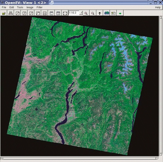
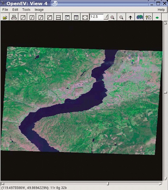
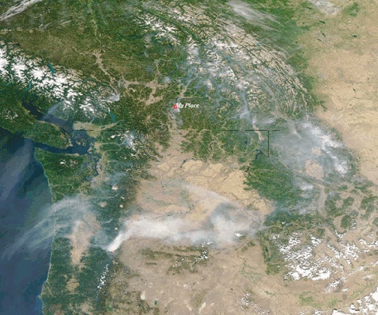
I used OpenEV to view the file and determine the area of interest. Figure 9-1 shows the whole image or scene.
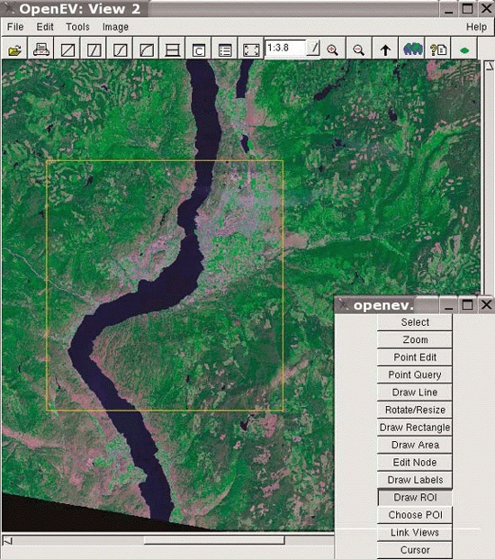
The large lake in the bottom half of the image is Okanagan Lake. After zooming in to the general area of interest, the Draw Region Of Interest (ROI) tool is used to select a rectangle. The Draw ROI tool is on the Edit Toolbar, which can be found in the Edit menu. To use the ROI tool, select the tool and drag a rectangle over the area. It creates an orange rectangle and leaves it on the screen, as shown in Figure 9-2.
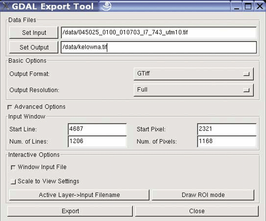
This area is then exported to a new file. To do this, use the File → Export tool. The Export window provides several options as shown in Figure 9-3. There is a small button near the bottom of the window that shows Advanced Options.
The filename of the image that will be created is entered into the Set Output box. This tool automatically exports the whole image to a new file, but only the selected region needs to be exported. To do this, select the Window Input File button. The four text entry boxes in the Input Window area show numbers that correspond to the pixel numbers of the image that will be exported. Only the pixels in the portion of the image identified as the ROI should be used.
Warning
A bug with the software sometimes requires you to redefine your ROI after the Window Input File option is selected. If you want to use the ROI that is already drawn, you can click on one edge of the ROI box in the view; the text boxes are then updated.
When you press the Export button, it creates the image using only the region you specify.
Now the original image isn’t needed, and the new image can be loaded into OpenEV. Figure 9-4 shows the new image being displayed.
Now you have a more manageable image to work with, and it is nicely clipped to the area of interest. You can clearly see changes in vegetation cover and urban areas. The urban areas are gray, thicker forests are a darker green, brighter green are thinned forests, etc. The data is fairly low resolution, but if you zoom in to the city you can almost find your way around the main streets. The lower part of the image shows some hilly landforms; this is the area of Okanagan Mountain Park, where the fire began. The image shows this area before the fire occurred.
This project will use a coordinate of a location from a GPS receiver. Because it is a single point, it is easy to just write down the coordinate off the receiver’s screen rather than exporting it to a file.
The point was recorded using latitude and longitude geographic coordinates. The image is in a different spatial reference system that uses the UTM projection. The coordinates can be converted into UTM, or the image can be transformed into geographic coordinates (e.g., decimal degrees). The latter can be easiest because you
may end up using other data from global datasets, which are typically stored in decimal degrees.
Use the GDAL utility gdalwarp
to transform the image. It is a Python script that can
transform rasters between different coordinate systems, often referred
to as reprojecting. The kelowna.tif image must be
removed from OpenEV before reprojecting.
Tip
GDAL utilities, including gdalwarp, are available in the
FWTools package. Instructions for acquiring and installing
FWTools can be found in Chapter
6.
The options for this command are formed in a similar way to
projection exercises elsewhere in this book (e.g., Chapter 7 and Appendix A). From the command line
specify the command name, the target spatial reference system
(-t_srs), and the source/target
filenames.
    >gdalwarp -t_srs "EPSG:4326" kelowna.tif kelowna_ll.tif

    Creating output file that is 1489P x 992L.
    :0...10...20...30...40...50...60...70...80...90...100 - done.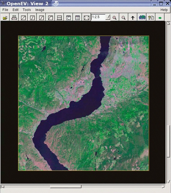
The EPSG code system is a shorthand way of specifying a projection and other coordinate transformation parameters. The EPSG code 4326 represents the lat/long degrees coordinate system. Otherwise, you would have to use the projection name and ellipsoid:
-t_srs "+proj=longlat +ellps=WGS84 +datum=WGS84"
Tip
To transform data between coordinate systems, programs such as
gdalwarp must know what the
source coordinate system is and what the output system will be. This
often requires the -s_srs (source
spatial reference system) option. Because the source image has this
coordinate system information already encoded into it, you don’t
need to explicitly tell gdalwarp
what it is. It will find the information in the file and
automatically apply it.
There is more information on projections, ellipsoids, and EPSG codes in Appendix A.
The resulting image looks slightly warped. Instead of being in UTM meter coordinates, all points on the map are in latitude/longitude decimal degree coordinates. Figure 9-5 shows the new image. When you move your cursor over the image, the coordinates show in the status bar at the bottom of the View window.
This image is now ready to use as a base map for creating your own data.
Starting to Draw Your Map Features
Once the base map is ready to be used, you can start to create new map data. This following example results in a simple map showing a home in Kelowna and the driving path to the fire burning in a nearby park. This involves a few different types of data: a point location of the home, a road line, and the area encompassing the fire.
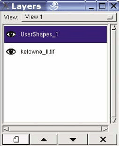
With OpenEV open and the satellite image as the background layer, you are almost ready to start drawing points (a.k.a. digitizing). First you need to create a new vector layer that will store the point locations. This is done by clicking the New Layer button in the Layers window. It is the bottom-left button that looks like a page, as shown in Figure 9-6.
When the new layer is created, it is given the default name
UserShapes_1. This layer is saved
as a shapefile. Shapefiles are limited to holding one type of data
at a time including points, lines, or polygons. If you create a
point, it only stores points. Right-click on the new layer, and
rename it Home in the properties window. You may need to turn the
layer off and back on for the title to change.
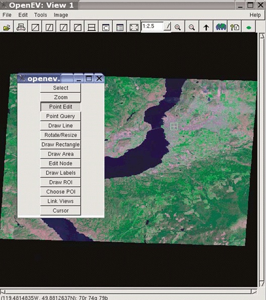
Next, open up the Edit Toolbar from the Edit menu. The tool called Point Edit allows you to draw points on the map and store them in the currently selected layer. In Figure 9-7, the tool was selected and then used to identify a location near downtown Kelowna. The location was based on the coordinate: 119.491°W, 49.882°N. To find this location, you move your pointer over the map and watch the coordinates in the status bar change. When you get to that coordinate, click the mouse button. The location is drawn as a green square, according to the default properties of the new layer.
To save the new location to a shapefile, make sure the layer
is still selected or active in the Layers window. From the File
menu, select Save Vector Layer. A dialog box pops up asking for the
location and name of the file to create. Store the file in the same
folder as the satellite image so they are easy to find. Call the
layer home.shp. To test that the
layer saved properly, turn off the new layer you have showing and
use File → Open to open
the shape file you just saved. To remove points or move existing
points, use the Select tool, and click on the point. You can click
and drag to move the point.
Creating and saving tabular attributes
The geographic location isn’t the only thing you’ll want to save. Sometimes you will want to save an attribute to identify the point later on.
Tip
An attribute is often called a field or column and is stored in the .dbf file associated with a shapefile.
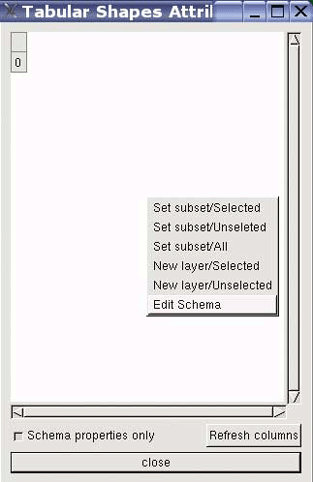
With the new layer selected, go to the Tools menu, and select
Tabular Shapes Grid. This shows an empty attribute table for the layer.
If you do this with another vector layer that already has
attributes, it will show those values. Your point will have a number
identifier (e.g., 0) but nothing
else to describe what the point represents. You can create a new
attribute by clicking inside the Tabular Shapes Attribute window. A menu pops up giving you the Edit Schema
option, as shown in Figure
9-8.
Warning
You can only edit the schema of a new layer—one that hasn’t been saved yet. It is often best to set up your attributes before saving the vector layer to a file.
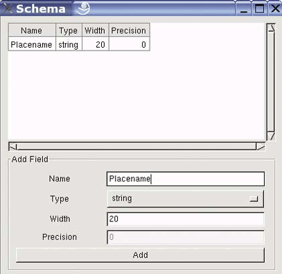
The Schema window that appears allows you to create a new attribute. In Figure 9-9 a new attribute has been created, called Placename. This is done by typing the name of the new attribute into the Name box near the bottom of the window, then pressing the Add button (leaving the default type as string and width as 20). The description of the attribute is listed at the top of the window.
Close the Schema window, and you are brought back to the
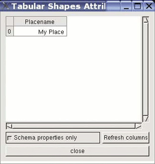
attribute listing. Now there is a new column, as in Figure 9-10. You can click
inside that column and type in a value for the Placename attribute
for the point created earlier. Try typing in My
Place and then press Enter
to save the change. This change is saved automatically, and no
manual resaving of the file is required.
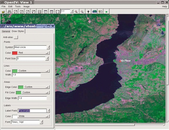
You can test out this attribute by using it to label your new point. To enable labels, right-click on the layer name in the Layers window. This brings up the properties of the layer. Now, select the Draw Styles tab. Near the bottom is an option called Label Field. You should be able to change this from disabled to Placename. As shown in Figure 9-11, your view window should now display the label for the point you created.
Now that you have a point showing where the house is you’re ready to draw some more details about the transportation infrastructure. This is a bit more complex because line features are more than just a point. In fact, line features are a series of points strung together and often referred to as line strings. Mapping road lines involves drawing a series of points for each line and saving them to a new shapefile.
Open the Layers window again, and click the New Layer button shown by the white-page icon. The typical new layer is created with a basic name such as UserShapes. Change the name to reflect the type of data being created, such as Roads.
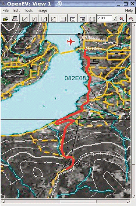
From the Edit Toolbar (activated under the Edit menu), you will find a Draw Line tool. This is much like the Point Edit tool, but is made for lines, not points. In this project, a line is drawn showing the rough driving path from a park to the house (My Place). A base map of the area from a government web site helps show where the driving path should be drawn.
With the additional base map showing road lines, you can now draw on top of those lines, following the path to the park. Figure 9-12 shows the rough red line drawn as a path. Each point clicked becomes a vertex in the line. OpenEV shows these as squares. After the last vertex is created, press the right mouse button to finish drawing. That line is now complete. You can modify the settings for the Roads layer to draw the line a bit thicker, making it easier to see on top of the busy base map. Note that the base map image is fairly poor resolution. That doesn’t matter because it will be tossed away when finished drawing; it’s used here as a temporary reference.
Now that you have a road line, you can save it to a shape file. As with the point data, just select that layer from the Layers window, and then use the Save Vector Layer option under the File menu to save it as roads.shp.
Mapping regions of interest (area/polygons data)
The third part of this mapping project is to draw the area of the forest fire. This won’t be a point or a line, but a polygon or area showing the extent of a feature. To help with this task, a few satellite images that were taken during or after the fire are used. Two main barriers come up, one of resolution and the other a lack of geo-referencing information. Both images and their shortcomings are presented to give you an idea of the thought process and the compromises that need to be made.
The first image is from http://rapidfire.sci.gsfc.nasa.gov/gallery/?2003245-0902/PacificNW.A2003245.2055.250m.jpg.
An overview of this image, with the point from home.shp, can be seen in Figure 9-13.
Tip
The web site at http://rapidfire.sci.gsfc.nasa.gov/gallery/ is a great resource! It includes various scales of real-time imagery showing thousands of events from around the globe.
The great thing about this image was that you can download the world file for the image too. This is the geo-referencing information needed to geographically position the image in OpenEV (and other GIS/mapping programs). The link to the world file is at the top of the page. Be sure to save it with the same filename prefix as the image. For these images, the filename suffix, or extension, is jgw. Be sure to save it with the proper name, or the image won’t find the geo-referencing information. The only problem with this image is that it’s very low resolution. My search for a better image led to:
It’s good and has much higher resolution, showing the fire very well, as seen in Figure 9-14.
This image isn’t geo-referenced. Because only the general
extent of the fire is needed, it isn’t worth the trouble of
geo-referencing. It is possible to do so using the gdal_translate utility with the -gcp option, but it can be very
tedious.
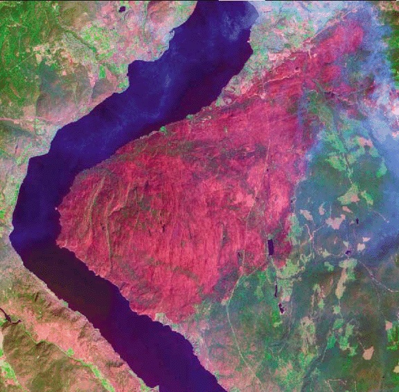
The final decision is to use the first image. It is lower resolution, but with little effort, it’s ready to work with OpenEV.
Add the fire image layer, and you will see that it overlaps the Kelowna Landsat image very well. Because the base data is no longer in UTM projection, it lines up with this image without any more effort. This image is fairly low resolution, but it does show the rough area of the fire as well as smoke from the eastern portion as it still burns.
Create a new layer to save the polygon data to, and call it Fire_Area. Then from the Edit Toolbar, select the Draw Area tool. Draw the outline of the burned area. Don’t be too worried about accuracy because the end product isn’t going to be a highly detailed map—just a general overview. Figure 9-15 shows the process of drawing the polygon.
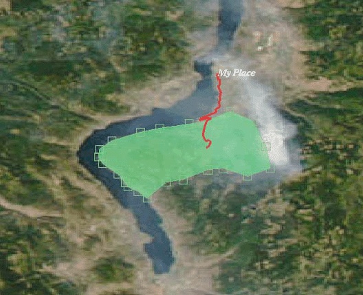
Each vertex helps to define the outer edge of the area. When done, press the right mouse button to complete the drawing. Then use Save Vector Layer to put the Fire_Area layer into a shape file called fire_area.shp.
Tip
You may notice that the extent of the fire shown on this image is quite different from the image in Figure 9-14. This is because Figure 9-15 was taken at an earlier time.
These examples have produced a few different images and three vector data shapefiles. These can now be used in a MapServer-based interactive web map (Chapters 10 and 11), or the data can be made available to others through a web service (Chapter 12). Either way, you have made the basic map data and have the flexibility to use it in any program that supports these data formats.