Table of Contents for

Web Mapping Illustrated

A simple world map boundary dataset will be used for this example. This shapefile contains boundaries of the country borders for the world and are available from the FreeGIS (http://www.freegis.org) web site at http://ftp.intevation.de/freegis/worlddata/freegis_worlddata-0.1_simpl.tar.gz.

The first thing to do is check out the data. This is done using the ogrinfo tool as described in Chapter 6. This isn’t a MapServer utility but is a valuable tool for getting started, as shown in Example 10-1.

                  > ogrinfo countries_simpl.shp -al -summary
INFO: Open of 'countries_simpl.shp'
using driver 'ESRI Shapefile' successful.

Layer name: countries_simpl
Geometry: Polygon
Feature Count: 3901
Extent: (-179.999900, -89.999900) - (179.999900, 83.627357)
Layer SRS WKT:
(unknown)
gid: Integer (11.0)
cat: Integer (11.0)
fibs: String (2.0)
name: String (255.0)
f_code: String (255.0)
total: Integer (11.0)

male: Integer (11.0)
female: Integer (11.0)
ratio: Real (24.15)

This example shows several key pieces of information prior to building the MapServer map file.

    Geometry: Polygon

The shapefile holds polygon data. MapServer can shade the polygon areas or just draw the outline of the polygons. If the geometry was line or linestring, it wouldn’t be possible to fill the polygons with a color.

    Feature Count: 3901

The feature count shows that there are many (3,901 to be exact) polygons in this file. If it said there were no features, that would tell me there is something wrong with the file.

    Extent: (-179.999900, -89.999900) - (179.999900, 83.627357)

ogrinfo shows that the data covers almost the entire globe, using latitude and longitude coordinates. The first pair of numbers describes the most southwestern corner of the data. The second pair of numbers describes the most northeastern extent. Therefore when making a map file, set it up so that the map shows the entire globe from -180,-90 to 180,90 degrees.

    Layer SRS WKT:
    (unknown)

There is no spatial reference system (SRS) set for this shapefile. By looking at the fact that the extent is shown in decimal degrees, it is safe to say that this file contains unprojected geographic coordinates.

    gid: Integer (11.0)
    cat: Integer (11.0)
    fibs: String (2.0)
    name: String (255.0)
    f_code: String (255.0)
    total: Integer (11.0)
    male: Integer (11.0)
    female: Integer (11.0)

This is a list of the attributes (or fields) that are part of the file. This is helpful to know when adding a label to your map to show, for example, the name of the country. It also indicates that the field called name holds up to 255 characters. Therefore some of the names can be quite long, such as "Macedonia, The Former Yugo. Rep. of".

With this information you are ready to put together a basic map file.

    > ogrinfo countries_simpl.shp -al | grep name | sort | uniqLayer name: countries_simpl
      name: String (255.0)
      name (String) = Afghanistan
      name (String) = Albania
      name (String) = Algeria
      name (String) = American Samoa
    continued...

The map file is the core of MapServer applications. It configures how the map will look, what size it will be, and which layers to show. There are many different configuration settings. Map file reference documents on the MapServer web site are a necessary reference for learning about new features. You can find the documents at http://mapserver.gis.umn.edu/doc/mapfile-reference.html.

Map files are simple text files that use a hierarchical, or nested, object structure to define settings for the map. The map file is composed of objects (a.k.a. sections). Each object has a keyword to start and the word END to stop. Objects can have other subobjects within them where applicable. For example, a map layer definition will include objects that define how layers will be drawn or how labels are created for a layer. Example 10-2 shows the most basic possible definition of a map file, using only 15 lines of text.

MAP                         # Start of MAP object
  SIZE 600 300
  EXTENT -180 -90 180 90
  LAYER                     # Start of LAYER object
    NAME countries
    TYPE POLYGON
    STATUS DEFAULT
    DATA countries_simpl
    CLASS                   # Start of CLASS object
      STYLE                 # Start of STYLE object
        OUTLINECOLOR 100 100 100
      END                   # End of STYLE object
    END                     # End of CLASS object
  END                       # End of LAYER object
END                         # End of MAP object and map file

There are only four objects in this map file:

Figure 10-1 is a graphical representation of the nested hierarchy of objects and properties.

Figure 10-1. Some of the main objects used in a MapServer map file

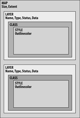
These objects are nested within each other. Each object has different types of settings. The SIZE and EXTENT settings are part of the MAP object. The LAYER object has a NAME, TYPE, STATUS, and DATA setting. The CLASS object has no settings in this example, but holds the STYLE object, which defines what OUTLINECOLOR to draw the lines.

The DATA setting gives the name of the dataset used for drawing this layer. In these examples, the data is a shapefile called countries_simpl. The examples assume that the map file is saved in the same location that you are running the commands from. For more information on other data formats and how to use them in MapServer, see Appendix B.

Comments can be interspersed throughout the map file using the # symbol. Everything written after the symbol, and on the same line, is ignored by MapServer. Example 10-2 uses comments to show the start and end of the main objects.

Indenting lines is optional but recommended to make your map file more readable. This structure is treated hierarchically by indenting the start of an object and un-indenting the end of the object.

Keywords in the map file can be upper, lower, or mixed case. It is recommended to write object names (such as MAP) and other keywords (such as DATA, COLOR) in uppercase and any items that are values for settings in lowercase (such as filenames, layer names, and comments). This is personal preference, but the convention can make it easier to read.

The text of the map file must be saved into a file on your filesystem. The filename of a map file must have a map suffix. The map file in Example 10-2 was saved as a file named global.map.

Values needing quotations can use either single or double quotes. In many cases, quotes are optional. Filenames are a good example. They can be either unquoted, single quoted, or double quoted.

The MapServer command shp2img takes the settings in the map file and produces a map image. Example 10-3 and the later Example 10-4 show the syntax of the command as well as an example of how to run it with the global.map map file.

> shp2img
Syntax: shp2img -m [mapfile] -o [image] -e minx miny maxx maxy
                -t -l [layers] -i [format]
  -m mapfile: Map file to operate on - required.
  -i format: Override the IMAGETYPE value to pick output format.
  -t: enable transparency
  -o image: output filename (stdout if not provided)
  -e minx miny maxx maxy: extents to render - optional
  -l layers: layers to enable - optional
  -all_debug n: Set debug level for map and all layers.
  -map_debug n: Set map debug level.
  -layer_debug layer_name n: Set layer debug level.

Only the first two options (-m and -o) are used in the following example:

    > shp2img -m global.map -o mymap.png

This example produces a new file called mymap.png, shown in Figure 10-2.

Figure 10-2. Initial map image of country boundaries

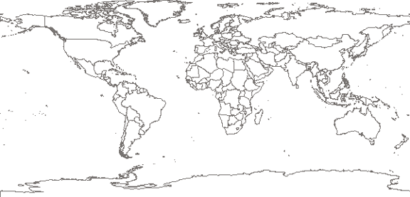
When the image is created, you can view it with any image viewing software. Internet web browsers can usually view PNG, JPEG, GIF, and others.

Depending on where you got MapServer from or how you compiled it, the images you produce might not be PNG format by default. To explicitly request PNG output files, use the -i option, like:

    > shp2img -m global.map -o mymap.png -i PNG

If you get an error or an image that isn’t viewable, your copy of MapServer might not support PNG output. If so, try a JPEG or GIF format. Make sure you change the file extension of the output image to reflect the image format you choose, for example:

    > shp2img -m global.map -o mymap.jpg -i JPEG

For more assistance see the Setting Output Image Formats section at the end of this chapter.

The simple map outline used in the previous example is great for new users. With some simple additions to the map file, you can easily add labels to your map. Example 10-4 shows the additional lines required to do this.

MAP
  SIZE 600 300
  EXTENT -180 -90 180 90
  LAYER
    NAME countries
    TYPE POLYGON
    STATUS DEFAULT
    DATA countries_simpl
    LABELITEM 'NAME'
    CLASS
      STYLE
        OUTLINECOLOR 100 100 100
      END
      LABEL
                  MINFEATURESIZE 40
                  END
    END
  END
END

Four more lines were add to the country LAYER object.

               
    LABELITEM 'NAME'

This setting tells MapServer what attribute to use to label the polygons. Each country polygon has a set of attributes that can be used to create labels. The LABELITEM setting specifies which one is used. ogrinfo, discussed in Chapter 7, can output a list of the attributes available in the file.

The additional lines were very simple:

               
    LABEL
        MINFEATURESIZE 40
    END

The second line is optional but makes the map more readable. There are a lot of ways to control how labels are drawn by MapServer. The MINFEATURESIZE option allowed me to specify a minimum size (number of pixels wide) that a country has to be before it will have a label created for it. Therefore smaller countries don’t get labeled because they would be unreadable at this scale anyway. Playing around with the value used for MINFEATURESIZE will yield very different results; try changing it from 40 to 20 or even down to 10.

If the EXTENT line is changed to zoom in to a smaller part of the world, more labels will show because the size of the countries will be larger.

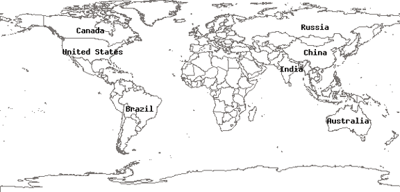
When you rerun the shp2img command as in Example 10-4, it now produces a world map with a few labels, as seen in Figure 10-3.

Figure 10-3. World map with country names as labels

The shp2img utility has several other options. One allows you to select a different map EXTENT to override what is defined in the map file. This is very handy because you don’t need to change the map file. Simply modify your command by adding the -e parameter and specify an extent as in the map file.

Before using the -e parameter you must choose an area to zoom in to. You can use the ogrinfo utility in concert with the ogr2ogr conversion tool. The ogrinfo command gives you only the overall extent of a given layer; it doesn’t report on the extent of a single feature. Therefore, you might want to extract only the features of interest and put them into a temporary shapefile. You can use the ogrinfo command on the new file and then throw the data away.

Example 10-5 shows an example of this utility assessing the extents of a country.

                  > ogr2ogr -where "name='Bulgaria'" bulgaria.shp countries_simpl.shp
                  > ogrinfo bulgaria.shp -al -summary

INFO: Open of 'bulgaria.shp'
using driver 'ESRI Shapefile' successful.

Layer name: bulgaria
Geometry: Polygon
Feature Count: 1
Extent: (22.371639, 41.242084) - (28.609278, 44.217640)
continued...

Using the -where option with ogr2ogr allows you to convert from one shapefile to a new one, but only transfer certain features, e.g., the boundary of Bulgaria. By running ogrinfo on that new file, you can see what Extent you should use in your map file to focus on that country. You can then use this extent in the shp2img command to create a map, as seen in Figure 10-4.

Figure 10-4. Zooming in to Bulgaria

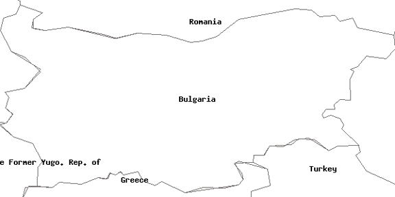
Here is an example that uses this information with the -e option:

    > shp2img -m global.map -o mymap.png -e 22.371639 41.242084 28.609278 44.217640

This map shows Bulgaria and some of the surrounding countries.

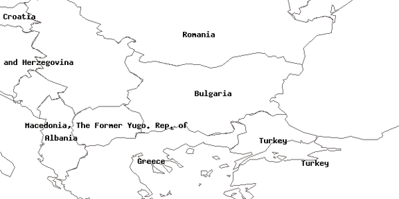
If you want to zoom out further, decrease the minimum coordinates (the first pair of numbers) and increase the maximum coordinates (the second pair) by one or two degrees like this:

    > shp2img -m global.map -o mymap.png -e 19 39 31 46

The map in Figure 10-5 is zoomed out further, giving a better context for Bulgaria.

Figure 10-5. Zooming out of a map image by changing the extent in the shp2img command

With a few more lines in the map file, as shown in Example 10-6, you can create a better looking map. Here is a modified map file with a few lines added and a couple changed.

MAP
  SIZE 600 300
  EXTENT -180 -90 180 90
  IMAGECOLOR 180 180 250
  LAYER
    NAME countries
    TYPE POLYGON
    STATUS DEFAULT
    DATA countries_simpl
    LABELITEM 'NAME'
   CLASSITEM 'NAME'
    CLASS
      EXPRESSION 'Bulgaria'
      STYLE

        OUTLINECOLOR 100 100 100
        COLOR 255 255 150
      END
      LABEL
        SIZE LARGE
                  MINFEATURESIZE 40
      END
    END
    CLASS
      EXPRESSION ('[NAME]' ne 'Bulgaria')
      STYLE
        OUTLINECOLOR 100 100 100
        COLOR 200 200 200
      END
    END
  END
END

The shp2img command is the same as in the previous example, but produces a colored map showing Bulgaria more clearly. The command is:

    > shp2img -m global.map -o example6b.png -e 19 39 31 46

The extent given by the shp2img command is still zoomed in to Bulgaria. Remember that the -e option overrides the EXTENT setting in the map file.

The result of this map file is shown in Figure 10-6.

Figure 10-6. Simple color theming of countries, highlighting a particular polygon and setting a background color

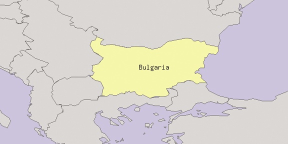
A few things to notice are three different COLOR settings and the single label:

               
    IMAGECOLOR 180 180 250

This setting basically makes any place blue where there were no country polygons in the shapefile. IMAGECOLOR is the background color of the map image, which is white by default. In this case it makes an interesting background simulating water.

You may notice that in the map file there are two CLASS...END objects. One tells how to color and label Bulgaria. The other tells how to color all the other countries.

               
    CLASSITEM 'NAME'

This line sets you up to use multiple classes in your map file. In this case, it says that the NAME attribute is going to be used to filter out certain features on the map. This is done by specifying an EXPRESSION (more on expressions in the next section) for each class, like in the first class:

    CLASS
       EXPRESSION 'Bulgaria'
       STYLE
          OUTLINECOLOR 100 100 100
          COLOR 255 255 150
       END
       LABEL
          SIZE LARGE
       END
    END

When drawing this class, MapServer draws only the polygons that have a NAME attribute of 'Bulgaria'. All other polygons or countries aren’t drawn in this class. The COLOR setting tells MapServer to fill Bulgaria with a color, and not just draw the outline as before. The only other change in this class is that the label size has been explicitly set a bit larger than the default.

The second class tells how to draw all countries other than Bulgaria.

               
    CLASS
       EXPRESSION ('[NAME]' ne 'Bulgaria')
       STYLE
         OUTLINECOLOR 100 100 100
         COLOR 200 200 200
       END
    END

Notice that there is a more complex expression set for this class. This one ignores Bulgaria but draws all the other countries. The next section discusses expression concepts in more detail.

The FILTER and EXPRESSION keywords can use simple or complex expressions to define the set of features to draw. Example 10-6 showed the simple way to use EXPRESSION to define the features for a CLASS . In the example, a single text string is provided. It is quoted, but doesn’t need to be. MapServer will look for all occurrences of that string in whatever attribute is set by CLASSITEM .

Logical expressions can also be defined where more than one value in a single attribute needs to be evaluated. Ranges of values and combinations of attributes can be given. Table 10-1 gives a summary of the types of expressions that can be used.

There are some exceptions to this table’s above rules when using the FILTER option with some data sources, particularly with database connections such as PostGIS:

Creating expressions isn’t always easy. Here are a few rules to keep in mind:

An important part of any map is the legend describing what colors and symbols mean. MapServer can create legends in realtime when a map is produced, or as a separate image.

To add a legend to your map, you must add a LEGEND...END object to your MAP. Note that this isn’t part of a LAYER object. It is part of the overall map object settings. Example 10-7 shows the first few lines of the map file (for context) with a few legend-specific settings highlighted.

MAP
  SIZE 600 300
  EXTENT -180 -90 180 90
  IMAGECOLOR 180 180 250

  LEGEND
    STATUS EMBED
    POSITION LR
    TRANSPARENT TRUE
  END
...

The status setting can be set to ON, OFF, or EMBED. The EMBED option is a great way to add the legend directly to the map. If you don’t use EMBED, then you must create the legend as a separate image (as you will see in a moment). Setting the legend to have a transparent background is also a nice option. If you don’t want it to be transparent, then you can remove the TRANSPARENT TRUE line. A default white background will be drawn behind the legend.

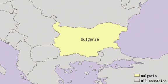
One more change is required to make the legend draw. You must have NAME settings for each class. The name given will be the text shown in the legend next to the symbols for that class. For example, add NAME 'Bulgaria' to the first class and NAME 'All Countries' to the second class as in Example 10-8. Until you do so, no legend will be created.

...
    CLASS
      NAME 'Bulgaria'
      EXPRESSION 'Bulgaria'

      STYLE
        OUTLINECOLOR 100 100 100
        COLOR 255 255 150
      END
      LABEL
        SIZE LARGE
        MINFEATURESIZE 40
      END
    END
    CLASS
      NAME 'All Countries'
      EXPRESSION ('[NAME]' ne 'Bulgaria')
      STYLE
        OUTLINECOLOR 100 100 100
        COLOR 200 200 200
      END
    END
...

Rerunning the shp2img command as before creates the image shown in Figure 10-7.

Figure 10-7. An embedded legend on the map

The POSITION setting has a few basic options that tell MapServer where to place the legend on the map using a two-letter code for the relative position: lower-right (LR), upper-center (UC), etc.

The legends so far have been embedded in the map image, but you can also create a separate image file that just includes the legend. This is done with the legend command:

               
    > legend global.map legend.png

The legend command creates an image that has just the legend in it as shown in Figure 10-8. It takes two parameters after the command name: first, the map file name and then the output image filename to be created.

Figure 10-8. A legend image created by the legend command

The legend is created according to the settings in the LEGEND object of the map file. You can change certain settings, but the POSITION and EMBED options are effectively ignored. Those options are intended for use with shp2img or with the mapserv web application.

A scale bar is a graphic showing the relative distances on the map. It consists of lines or shading and text describing what distance a segment of line in the scale-bar represents. As with legends in the preceding examples, it is simple to add scale-bar settings to your map file. All the options for scale-bar settings are listed in the MapServer map file documentation, under the scale-bar object at http://mapserver.gis.umn.edu/doc/mapfile-reference.html#scalebar.

Example 10-9 highlights the eight lines added to the map file in previous examples.

MAP
  SIZE 600 300
  EXTENT -180 -90 180 90
  IMAGECOLOR 180 180 250

  UNITS DD

  SCALEBAR
    STATUS EMBED
    UNITS KILOMETERS
    INTERVALS 3
    TRANSPARENT TRUE
    OUTLINECOLOR 0 0 0
  END

  LEGEND
    STATUS EMBED
...

A scale bar converts the map distances (centimeters, inches, pixels) to real-world distances (kilometers, miles), as seen in the lower-left corner of Figure 10-9.

Figure 10-9. Map image with an embedded scale bar

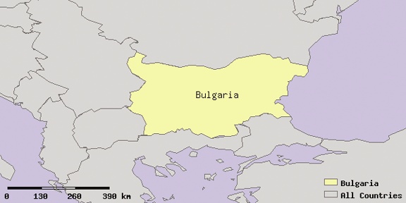
The same method used in previous examples using shp2img created this map with the embedded scale bar:

    > shp2img -m global.map -o mymap.png -e 19 39 31 46

The first line added to the map file is the UNITS keyword. DD tells MapServer that the mapping data is represented in decimal degree coordinates/units. This setting affects the whole map file and isn’t just scale bar-specific, which is why it isn’t inside the SCALEBAR...END object.

The SCALEBAR object of the map file has several options. A few, but not all, of the options are used in this example. These are just enough to make a nice-looking scale bar without a lot of fuss. The STATUS EMBED option is just like the one used in the legend example earlier. It puts the graphic right on the map, rather than requiring you to create a separate graphic. The UNITS KILOMETERS specifies what measurement units are shown on the scale bar. In this case each segment of the scale bar is labeled in kilometers. This can be changed to inches, feet, meters, etc.

INTERVALS 3 makes three segments in the scale bar. The default is four segments. This is a handy option, allowing you to have control over how readable the resulting scale bar is. If you have too many segments crammed into a small area, the labels can become hard to read.

There is one important option not shown in the earlier example. SIZE x y is an option that explicitly sets the width (x) and height (y) of the scale bar. You can accept the default to keep it simple. Note that when specifying the number of segments using INTERVALS, it subdivides the width accordingly. If you want a large number of INTERVALS, you will probably need to increase the SIZE of the scale bar to make it readable.

The last two options in Example 10-9 are aesthetic. TRANSPARENT makes the background of the scale bar clear. OUTLINECOLOR creates a thin black outline around the scale bar segments.

If you don’t want to embed the scale bar in your map, change STATUS EMBED to STATUS ON and use the scalebar command-line utility to create a separate graphic image. It is used like the legend utility in previous examples. The following example shows how you use the command:

    > scalebar global.map scalebar.png

The command takes two parameters, a map filename and an output image name. Note that scalebar doesn’t have the same options as shp2img.

Figure 10-10 shows the image created by the command.

Figure 10-10. A simple scale bar graphic produced by a map file and the scalebar utility

Be sure not to scale the graphics if you are going to manually pull together the scale bar and map images for something like a publication or web page. If you change the size or scale of the scale bar and don’t adjust the map image accordingly, your scale bar will be inaccurate.

The final map file created for this example is shown in Example 10-10. The EXTENT value has been changed to reflect the extents used in the shp2img command in earlier examples.

MAP                         # Start of MAP object
  SIZE 600 300              # 600 by 300 pixel image output
  #EXTENT -180 -90 180 90   # Original extents ignored
  EXTENT 19 39 31 46        # Final extents
  IMAGECOLOR 180 180 250    # Sets background map color
  UNITS DD                  # Map units
  SCALEBAR                  # Start of SCALEBAR object
    STATUS EMBED            # Embed scalebar in map image
    UNITS KILOMETERS        # Draw scalebar in km units

    INTERVALS 3             # Draw a three piece scalebar
    TRANSPARENT TRUE        # Transparent background
    OUTLINECOLOR 0 0 0      # Black outline
  END                       # End of SCALEBAR object
  LEGEND                    # Start of LEGEND object
    STATUS EMBED            # Embed legend in map image
    POSITION LR             # Embed in lower-right corner
    TRANSPARENT TRUE        # Transparent background
  END                       # End of LEGEND object
  LAYER                     # Start of LAYER object
    NAME countries          # Name of LAYER
    TYPE POLYGON            # Type of features in LAYER
    STATUS DEFAULT          # Draw STATUS for LAYER
    DATA countries_simpl    # Source dataset
    LABELITEM 'NAME'        # Attribute for labels
    CLASSITEM 'NAME'        # Attribute for expressions
    CLASS                   # Start of CLASS object
      NAME 'Bulgaria'       # Name of CLASS
      EXPRESSION 'Bulgaria' # Draw these features in class
      STYLE                 # Start of STYLE object
        OUTLINECOLOR 100 100 100
                            # Color of outer boundary
        COLOR 255 255 150   # Polygon shade color
      END                   # End of STYLE object
      LABEL                 # Start of LABEL object
        SIZE LARGE          # Size of font in label
        MINFEATURESIZE 40   # Min. sized polygon to label
      END                   # End of LABEL object
    END                     # End of CLASS object
    CLASS                   # Start of CLASS object
      NAME 'All Countries'  # Name of CLASS
      EXPRESSION ('[NAME]' ne 'Bulgaria')
                            # Draw features in class
      STYLE                 # Start of STYLE object
        OUTLINECOLOR 100 100 100
                            # Color of outer boundary
        COLOR 200 200 200   # Polygon shade color
      END                   # End of STYLE object
    END                     # End of CLASS object
  END                       # End of LAYER object
END                         # End of MAP object and map file