Table of Contents for
Web Mapping Illustrated
 Web Mapping Illustrated
Published by
O'Reilly Media, Inc., 2005
Web Mapping Illustrated
Published by
O'Reilly Media, Inc., 2005
- Web Mapping Illustrated
- Cover
- Web Mapping Illustrated
- A Note Regarding Supplemental Files
- Foreword
- Preface
- Youthful Exploration
- The Tools in This Book
- What This Book Covers
- Organization of This Book
- Conventions Used in This Book
- Safari Enabled
- Comments and Questions
- Acknowledgments
- 1. Introduction to Digital Mapping
- 1.1. The Power of Digital Maps
- 1.2. The Difficulties of Making Maps
- 1.3. Different Kinds of Web Mapping
- 2. Digital Mapping Tasks and Tools
- 2.1. Common Mapping Tasks
- 2.2. Common Pitfalls, Deadends, and Irritations
- 2.3. Identifying the Types of Tasks for a Project
- 3. Converting and Viewing Maps
- 3.1. Raster and Vector
- 3.2. OpenEV
- 3.3. MapServer
- 3.4. Geospatial Data Abstraction Library (GDAL)
- 3.5. OGR Simple Features Library
- 3.6. PostGIS
- 3.7. Summary of Applications
- 4. Installing MapServer
- 4.1. How MapServer Applications Operate
- 4.2. Walkthrough of the Main Components
- 4.3. Installing MapServer
- 4.4. Getting Help
- 5. Acquiring Map Data
- 5.1. Appraising Your Data Needs
- 5.2. Acquiring the Data You Need
- 6. Analyzing Map Data
- 6.1. Downloading the Demonstration Data
- 6.2. Installing Data Management Tools: GDAL and FWTools
- 6.3. Examining Data Content
- 6.4. Summarizing Information Using Other Tools
- 7. Converting Map Data
- 7.1. Converting Map Data
- 7.2. Converting Vector Data
- 7.3. Converting Raster Data to Other Formats
- 8. Visualizing Mapping Data in a Desktop Program
- 8.1. Visualization and Mapping Programs
- 8.2. Using OpenEV
- 8.3. OpenEV Basics
- 9. Create and Edit Personal Map Data
- 9.1. Planning Your Map
- 9.2. Preprocessing Data Examples
- 10. Creating Static Maps
- 10.1. MapServer Utilities
- 10.2. Sample Uses of the Command-Line Utilities
- 10.3. Setting Output Image Formats
- 11. Publishing Interactive Maps on the Web
- 11.1. Preparing and Testing MapServer
- 11.2. Create a Custom Application for a Particular Area
- 11.3. Continuing Education
- 12. Accessing Maps Through Web Services
- 12.1. Web Services for Mapping
- 12.2. What Do Web Services for Mapping Do?
- 12.3. Using MapServer with Web Services
- 12.4. Reference Map Files
- 13. Managing a Spatial Database
- 13.1. Introducing PostGIS
- 13.2. What Is a Spatial Database?
- 13.3. Downloading PostGIS Install Packages and Binaries
- 13.4. Compiling from Source Code
- 13.5. Steps for Setting Up PostGIS
- 13.6. Creating a Spatial Database
- 13.7. Load Data into the Database
- 13.8. Spatial Data Queries
- 13.9. Accessing Spatial Data from PostGIS in Other Applications
- 14. Custom Programming with MapServer’s MapScript
- 14.1. Introducing MapScript
- 14.2. Getting MapScript
- 14.3. MapScript Objects
- 14.4. MapScript Examples
- 14.5. Other Resources
- 14.6. Parallel MapScript Translations
- A. A Brief Introduction to Map Projections
- A.1. The Third Spheroid from the Sun
- A.2. Using Map Projections with MapServer
- A.3. Map Projection Examples
- A.4. Using Projections with Other Applications
- A.5. References
- B. MapServer Reference Guide for Vector Data Access
- B.1. Vector Data
- B.2. Data Format Guide
- ESRI Shapefiles (SHP)
- PostGIS/PostgreSQL Database
- MapInfo Files (TAB/MID/MIF)
- Oracle Spatial Database
- Web Feature Service (WFS)
- Geography Markup Language Files (GML)
- VirtualSpatialData (ODBC/OVF)
- TIGER/Line Files
- ESRI ArcInfo Coverage Files
- ESRI ArcSDE Database (SDE)
- Microstation Design Files (DGN)
- IHO S-57 Files
- Spatial Data Transfer Standard Files (SDTS)
- Inline MapServer Features
- National Transfer Format Files (NTF)
- About the Author
- Colophon
- Copyright
The Third Spheroid from the Sun
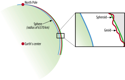
The Earth is round, or so they say. Video games, globes, and graphic art may depict the Earth as a perfect ball shape or sphere, but in reality the Earth is a bit squished. Therefore, we call the Earth a spheroid, rather than a sphere. It is sphere-like, but somewhat elliptical.
To take it one level further, we all know that the surface of the Earth isn’t perfectly uniform. There are mountains and valleys, bumps and dips. Geoid is the term used for a more detailed model of the Earth’s shape. At any point on the globe, the geoid may be higher or lower than the spheroid. Figure A-1 shows an example of the relationships among the sphere, spheroid, and geoid.
Figure A-1 is based on a graphic courtesy of Dylan Prentiss, Department of Geography, University of California, Santa Barbara. Further descriptions are available at the Museum’s Teaching Planet Earth web site, http://earth.rice.edu/mtpe/geo/geosphere/topics/remotesensing/60_geoid.html.
As you can see, when talking about the shape of the Earth it is very important to know what shape you are referring to. The shape of the Earth is a critical factor when
producing maps because you (usually) want to refer to the most exact position possible. Many maps are intended for some sort of navigational purpose, therefore mapmakers need a consistent way of helping viewers find a location.
Geographic Coordinate System
How do you refer someone to a particular location on the Earth? You might say a city name, or give a reference to a landmark such as a mountain. This subjective way of referring to a location is helpful only if you already have an idea of where nearby locations are. Driving directions are a good example of a subjective description for navigating to a particular location. You may get directions like “Take the highway north, turn right onto Johnson Road and go for about 20 miles to get to the farm.” Depending on where you start from, this may help you get to the farm, or it may not. There has to be a better way to tell someone where to go and how to get there. There is a better way; it is called the Geographic Coordinate System.
The increasing use of hand-held Global Positioning Systemreceivers is helping the general public think about the Geographic Coordinate System. People who own a GPS receiver can get navigation directions to a particular location using a simple pair of numbers called coordinates . Sometimes an elevation can be provided too, giving a precise 3D description of a location.
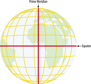
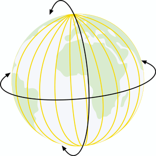
A Geographic Coordinate System, like that shown in Figure A-2, is based on a method of describing locations using a longitude and latitude degree measurement. These describe a specific distance from the equator (0° north/south) and the Greenwich Meridian (0° east/west).
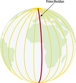
From this starting point, the earth is split into 360 slices, running from the North Pole to the South Pole, known as degrees and represented by the symbol °. Half of
these slices are to the east of 0° and half are to the west. These are referred to as longitudes or meridians . Therefore, the maximums are 180° west longitude and 180° east longitude (see Figure A-3).
A variant of the basic geographic coordinate system for longitudes is useful in some parts of the world. For example, 180° west longitude runs right through the South Pacific Islands. Maps of this area can use a system where longitudes start at 0° and increase eastward only, ending back at the same location which is also known as 360° (see Figure A-4).
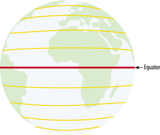
The earth is divided into latitudes as well. You can picture these as 180 slices running horizontally around the globe. Half of these slices are north of the equator and the other half are south of the equator. These are referred to as latitudes or parallels. Therefore the values range from 90° south latitude (at the south pole) to 90° north latitude (at the north pole) (see Figure A-5).
Decimal degrees versus degrees minutes seconds
Global coordinates can be represented using a couple of different notations. It is hard to say if one of them is more common than the other, but some are certainly more intuitive than others.
One of the more traditional notations is known as Degrees Minutes Seconds (DMS). The coordinates are written as three separate numbers, each representing a degree, minute, and second, respectively.
For example, 122°W is read
as 122 degrees west. Rarely are the degrees alone precise enough for
a location; minutes and seconds are subdivisions of each degree and
provide more precision. Each minute is 1/60th of a degree. Likewise,
one second is 1/60th of a minute. A more precise example would be
122°30'15"W, read as 122 degrees,
30 minutes, and 15 seconds west.
At the other end of the spectrum is the decimal degree (DD)
notation. This notation uses a decimal place in place of minutes and
seconds. For example, 122.525°W
is read as 122.525 degrees west.
The decimal portion, .525,
represents just over half a degree.
In between DMS and DD are a couple more permutations. One of
the more common is to have a degree and a minute, but the seconds
are a decimal of the minute; for example, 122°30.25". I find this type of notation
difficult to use because it mixes two worlds that don’t play well
together. It can’t be called either DD or DMS, making it tough to
explain. I highly recommend using Decimal Degrees as much as
possible. It is commonly understood, supported well by most tools
and is able to be stored in simple numeric fields in
databases.
It is also common to see different signs used to distinguish
an east or west value. For example, 122°W may also be known as -122° or simply -122; this is minus because it is less
than or west of the Greenwich Meridian. The opposite version of it,
e.g., 122°, is assumed to be
positive and east of 0°.
Map Projections: Flattening the Spheroid
The Geographic Coordinate System is designed to describe precise locations on a sphere-like shape. Hardcopy maps and onscreen displays aren’t at all sphere-like; hence they present a problem for making useful depictions of the real world. This is where map projections come in. The problem of trying to depict the round earth on a flat surface is nothing new, but the technology for doing so has improved substantially with the advent of computerized mapping.
The science of map projections involves taking locations in a Geographic Coordinate System and projecting them on to a flat plane. The term projection tells a little bit about how this was done historically. Picture a globe that is made of glass. Painted on the glass are the shapes of the continents. If you were to put a light inside the glass, some light would come through and some would be stopped by the paint. If you held a piece of paper up beside the globe, you would see certain areas lit up and other areas in shadow. You would, in fact, see a projected view of the continents, much like a video projector creates from shining light through a piece of film. You can sketch the shapes on the paper, and you would have a map. Projections are meant for display on a flat surface. Locating a position on a projected map requires the use of a planar coordinate system (as opposed to a geographic coordinate system). This is considered planar because it is a simple plane (the flat paper) and can only touch one area on the globe.
This example has limitations. You can map only the portion of the earth that is nearest the paper, and continents on the other side of the globe can’t be mapped on the same piece of paper because the light is shining the other way. Also, the map features look most accurate close to the center of the page. As you move outward from the center, the shapes get distorted, just like your shadow late on a summer day as it stretches across the sidewalk: it’s you, but not quite right. More inventive ways of projecting include all sorts of bending and rolling of the paper. The paper in these examples can be referred to as a plane: the flat surface that the map is going to be projected on to.
There are many different classes and types of map projections. Here are just a few of the most simple:
- Cylindrical projections
These involve wrapping the plane around the globe like a cylinder. They can touch the globe all the way around, but the top and bottom of the map are distorted.
- Conic projections
These look like, you guessed it, a plane rolled into a cone shape and set like a hat onto the globe. If you set it on the top of the globe, it rests on a common latitude all the way around the North Pole. The depth of the cone captures the details of the pole, but are most accurate at the common latitude. When the paper is laid flat, it is like removing the peel of an orange and laying it perfectly flat.
- Orthographic projections
These look like a map drawn by an astronaut in orbit. Instead of having the light inside the globe, it’s set behind the globe; the paper is flat against the front. All the features of the continents are projected onto the paper, which is hardly useful for a global-scale map because it shows only a portion of the globe. However, if the features on the backside are ignored, then it looks like a facsimile of the earth. With the current processing power of computers, rendering maps as spheres is possible, but these realistic-looking perspectives aren’t always useful.
The role of mathematical computations is essential to projecting map data. It is the heart of how the whole process works. Fortunately, you don’t need to know how it works to use it. All you need to know is that the glass-globe analogy is, in fact, replaced by mathematical calculations.
Each map projection has strong and weak points. Different types of projections are suited for different applications. For example, a cylindrical projection gives you an understandable global map but won’t capture the features of the poles. Likewise a conic projection is ideal for polar mapping, but impossible for global maps.
Although there are a few main classes of projections (cylindrical, conic, etc.) there are literally hundreds of projections that have been designed. The details of how each one is implemented vary greatly. In some cases, you simply need to know what map projection you want. In others, you need to know detailed settings for where the plane touches the globe or at what point the map is centered.
Planar/Projected Coordinate System
Both planar and projected are terms that describe the coordinate system designed for a flat surface. The Geographic Coordinate System uses measurements based on a spherical world, or degrees. A projected coordinate system is designed for maps and uses a Cartesian Plane to locate coordinates.
The Cartesian Plane is a set of two (or more) axes where both axes intersect at a central point. That central point is coordinate 0,0. The axes use common units and can vary from one map projection to another. For example, the units can be in meters: coordinate (100,5) is 100 meters east and 5 meters north. Coordinate (-100,-5) is 100 meters west and 5 meters south.
The Y axis is referred to as the central meridian. The central meridian could be anywhere and depends on the map projection. If a projection is localized for Canada, the central meridian might be 100° west. All east/west coordinates would be relative to that meridian. This is in contrast to the geographic coordinate system where the central meridian is the Greenwich Meridian, where all east/west coordinates are always relative to the same longitude.
The X axis is perpendicular to the Y axis, meeting it at a right angle at 0,0. This is referred to as the latitude of origin. In a projected coordinate system, it can be any latitude. If focused on Canada, the latitude of origin might be 45° north. Every projected north/south coordinate is relative to that latitude. In the geographic coordinate, this is the equator, where all north/south coordinates are always relative to the equator.