Web Mapping Illustrated

Using OpenEV

OpenEV was designed as an example of the kinds of tools that can be built on top of various open source GIS libraries. It has a variety of powerful features, is open to complete customization, and includes the ability to add in custom tools written in Python. For the purposes of this chapter, only some of the basic functions (not including Python scripting) will be demonstrated. These include the ability to view various formats of raster and vector data layers, change their colors, create labels, etc. It is also possible to create your own data; check for that in Chapter 9.

Follow along with the examples, and try them yourself to build up your familiarity and comfort with this tool. You will first test your installation of OpenEV, then create some custom maps using the demonstration datasets. Once the basic viewing capabilities are explored, you will learn to create some more sophisticated color classifications, and ultimately produce a 3D model to navigate through.

Installing OpenEV

Chapters 5 and 6 walked you through how to acquire sample data and review it using some simple tools. If you don’t already have the MapServer demonstration data and the FWTools downloaded and installed, please refer back to these sections in Chapter 6.

You should have two things: a sample MapServer application known as Workshop and a copy of OpenEV that comes with FWTools. To test that you have OpenEV installed, launch the program. Windows users will launch the OpenEV_FW desktop shortcut. This will open a command window and create some windows.

Warning

Don’t close the command window that appears. OpenEV needs this to stay open. It is safe to minimize the window while using OpenEV.

Linux users will launch the openev executable from the FWTools bin_safe folder.

Tip

Linux users: if you don’t have a bin_safe folder, run the installer by typing:

    > ./install.sh

This prepares the installation and creates a folder called bin_safe. Now, run the command:

    > . /fwtools_env.sh

(Note the space after the period.) This loads all the environment variables. Now you should be able to run openev from anywhere.

When starting, the main window titled “OpenEV: View 1” should appear with a black background. The Layers windows will also appear.

Loading Sample Map Data into OpenEV

Starting from the default View 1 screen, you can add in sample data by selecting Open from the File menu, or by clicking on the folder icon on the left side of the main tool bar. The File Open window allows you to find a dataset on your filesystem and load it as a layer in OpenEV. All files are listed in the File Open window, whether or not they are spatial datafiles. OpenEV doesn’t attempt to guess what they are until you actually try to open one.

Windows users may get confused when trying to find data on a drive with a different drive letter. The drive letters are listed below all the folders in the File Open window. You must scroll down to find them.

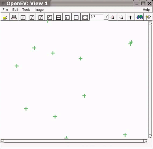
Open the Airports Shapefile

Navigate using the File Open window to the location where the workshop/data folder has been unzipped. In the data folder, you will see dozens of files listed. Select airports.shp to load the airports shapefile. As shown in Figure 8-1, 12 small green crosses should appear in the view. Each point represents the location of an airport from the demonstration dataset.

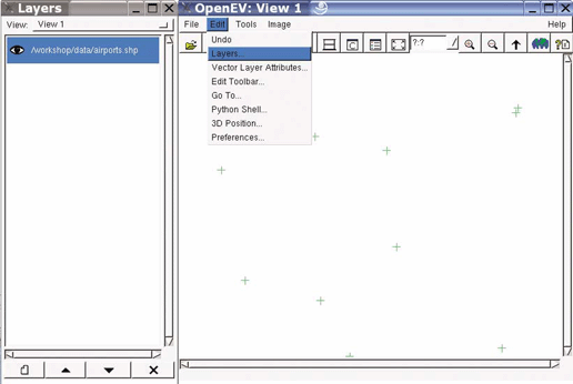
Using the Layers Window

OpenEV has other windows for different tasks. One of these is the Layers window. If it isn’t already showing, select Layers from the Edit menu, as shown in Figure 8-2. This window lists the layers that are currently loaded into OpenEV. A layer can be an image or, as in our case, vector data. Only the airports layer should be loaded at this point. You will see the full path to the airports.shp file. Beside this layer name is an eye icon. This says that the layer is currently set to be visible in the view. Try clicking it on and off.

Figure 8-1. Initial loading of airport shape file

The layers window allows you to change certain graphical display settings for your layers. Access these settings by right-clicking on the layer name. The airport layer name may be somewhat obscured if you have the file deep in subfolders, because the default name for the layer is the whole path to the file. The layer window can be resized to show the full name more clearly if necessary.

Changing General Layer Settings

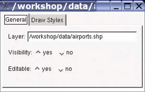
Right-click on the airports layer in the Layers window, you’ll see the Properties window for the airports layer, as shown in Figure 8-3.

There are three options on the General tab of the Properties window:

Layer

This is the layer name. It can be changed to whatever you want it shown as in the Layers window. Changing this value won’t affect the datafile itself. Because the default puts the whole path in as the layer name, change this to something

Figure 8-2. Viewing the layers loaded into the view

Figure 8-3. General layer settings window

more meaningful, such as “Airports”. It will be updated in the Layers window the next time the layer is turned off and back on.

Visibility

This setting is changed when clicking on the eye icon in the layers window. When set to Yes, the layer shows in the view. Otherwise, it is turned off and won’t be drawn.

Editable

Vector data files can be edited within OpenEV. This is a powerful feature that is often hard to find in free programs. Setting a layer to be editable allows you to move features around, create new ones, delete them, or reshape lines. The default setting is Yes. It is a good habit to change it to No so that you don’t accidentally modify features.

Changing Draw Styles for Layers

The other tab at the top of the airports Properties window is called Draw Styles. Switch to this tab to see the various draw settings, as shown in Figure 8-4. There are five different groups of settings on this tab.

Figure 8-4. Draw styles window

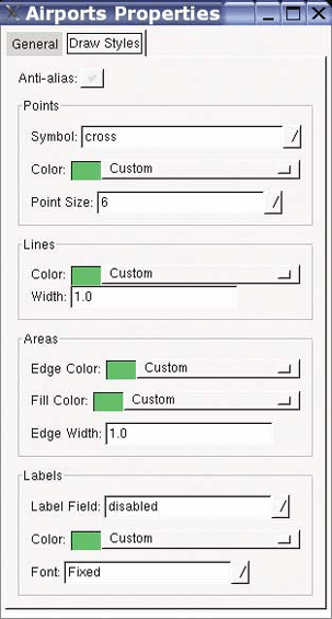
Anti-alias: The anti-alias setting is a checkbox; it is either on or off (it is off by default). This option allows your map features to be drawn more smoothly. It can often make your text and shapes look softer and less stark. The graphics of the airport layer points are pretty simple. Using anti-aliasing won’t make much difference. It is most noticeable with curved lines or text.
Points: Every airport point is given a specific symbol on the map. In this case, the airports are shown with the default symbol, a cross. There are several other options, and all are very simple. By default they are colored green; you can change the color by clicking on the word Custom or on the drop-down box square beside Custom. This provides a list of colors to choose from. Try some out, or select Custom from the list, and you are shown a color wheel. Note that the color wheel has an opacity setting that allows you to set the amount of transparency for your layer. Point size sets the size of the symbol on the map; this can be chosen from the drop-down list or typed in.
Lines: The settings for lines are fairly simple. You can set only the width and color.
Areas: Polygon features are also known as areas. Area features are made up of an edge line that draws the perimeter of the feature. It is possible to give that edge line a color and a width. You can also choose what color will fill the inside of the feature.
Labels: In many datasets, point features and label features look and act the same: they have a specific (point-like) location and some text associated with them. The text is shown for a layer when the Label Field is set. By default, it is disabled, and no labels are drawn. If the point dataset you are working with has attributes or fields of data for each point, you can select one from this list. With the airports layer, try setting the Label Field to NAME. This shows the name of each airport beside the point. Note that labels can’t be drawn for line or area layers at this time.

When all the settings are complete, simply close the properties window by clicking on the X symbol in the top-right corner of the window. As you change settings, they are updated automatically in the view. Close the properties window, and return to the View 1 window.

Adding More Data to the View

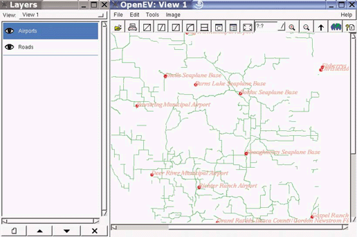
One of the benefits of software like OpenEV is the ability to add many layers of data and compare them with each other. With some work setting draw styles, a simple map can be produced. The workshop dataset includes more than just an airports layer.

Click on the folder icon in View 1 to add another layer of features. The data is located in the same folder as the airports. This time add the file called ctyrdln3.shp. This is a layer containing road line data for the same county as the airports.

From the Layers window, right-click on the ctyrdln3 layer to open the layer properties window. Change the name to something obvious, such as Roads. You should also change the road line colors so they aren’t the same as the airports. Notice that the road lines are being drawn on top of the airport symbols. The order of the layers is always important when creating a map, and, depending on your project, you may want to reorder the layers. This is done in the Layers window. Left-click on the layer name you want to change. The layer name will now be highlighted. Then select one of the up or down arrow buttons at the bottom of the Layers window. This moves the layer up or down in the draw order. The final product looks like Figure 8-5.

Figure 8-5. Road lines and airports loaded

Previous Chapter

8.1. Visualization and Mapping Programs

Next Chapter

8.3. OpenEV Basics