Web Mapping Illustrated

Spatial Data Queries

One of the strengths of PostGIS is its ability to store spatial data in a mature, enterprise-level, relational database. Data is made available through standard SQL queries, making it readily available to do analysis with another program without having to import and export the data into proprietary data formats. Another key strength is its ability to use spatially aware PostGIS functions to perform the analysis within the database, still using SQL. The spatial data query examples in this section are the most basic possible. PostGIS boasts of a variety of operators and functions for managing, manipulating, and creating spatial data, including the ability to compute geometric buffers, unions, intersections, reprojecting between coordinate systems, and more. The basic examples shown here focus on loading and accessing the spatial data.

To see what data is in the countyp020 table, you can use any basic SQL query to request a listing. For example, this typical SQL query lists all data in the table, including the very lengthy geometry definitions. Running this query isn’t recommended:

# SELECT * FROM countyp020;

Getting a list of over 6,000 counties and their geometries would hardly be useful. A more useful query might be something like Example 13-3 which limits and groups the results.

Example 13-3. A basic SELECT DISTINCT query to list the counties in New Mexico state

# SELECT DISTINCT county FROM countyp020 WHERE state = 'NM';
             county
---------------------------------
 Bernalillo County
 Catron County
 Chaves County
 Cibola County
 Colfax County
 Curry County
 DeBaca County
 Dona Ana County
 Eddy County
 Grant County
 Guadalupe County
 Harding County
 Hidalgo County
 Lea County
 Lincoln County
...
 (33 rows)

This query lists all the counties in the state of New Mexico (state = 'NM'). This has nothing to do with the spatial data, except that all this information was originally in the shapefile that was loaded. To see some of the geographic data, you must run a query that returns this information.

Example 13-4 shows a query that lists all the information about Curry County, including a list of all the geometric points used to define the shape of the county.

Tip

At the beginning of this example the \x command tells psql to list the data in expanded display mode. This is a bit easier to read when there is a lot of data and very few records. Using \x a second time disables expanded mode.

Example 13-4. Querying a table to show all the geometric and tabular data for a particular feature

project1=# \x
Expanded display is on.
project1=# SELECT * FROM countyp020 WHERE state='NM' AND county = 'Curry County';
 
[ RECORD 1 ] -------------------------------------------
ogc_fid      | 4345
wkb_geometry | SRID=-1;POLYGON((-103.04238129 34.74721146,
-103.04264832 34.36763382,-103.04239655 34.30997849,
-103.0424118 34.30216599,-103.73503113 34.30317688,
-103.49039459 34.77983856...))
area         | 0.358
perimeter    | 2.690
countyp020   | 4346
state        | NM
county       | Curry County
fips         | 35009
state_fips   | 35
square_mil   | 1404.995

Tip

More recent versions of PostGIS don’t display the geometry as text by default. To have it display coordinates in text format, you must use the astext() function with the wkb_geometry column like:

SELECT astext(wkb_geometry) FROM...

Some of the geometry information has been removed because the list of coordinates is very long; there is one pair of coordinates for every vertex in the polygon. This example shows how you can access spatial coordinate data directly with your queries. No GIS program is required to get this level of information, just basic SQL. The results may not be in the format you need, but you can modify it to suit your purposes. For example, if you are creating a custom application that needs access to geographic coordinates, you can call a PostgreSQL database, access the geometry of a table, then manipulate the data into the form your application needs.

Most people interested in web mapping don’t need to create their own custom application for accessing and using the power of PostGIS. MapServer, for example, can query PostGIS for the geometry of these features and display it on a map. You only need to know how to point MapServer to the right database and table. More on using MapServer with PostGIS follows later in this chapter.

Building Spatial Indexes

Before doing spatial queries, some preparation work is needed. To improve spatial query performance, you should build spatial indexes for any tables that hold geometry data. This is done using the CREATE INDEX command with a few geometry options. The command to create an index for the geometry in the countyp020 table looks like this:

# CREATE INDEX idx_countyp020_geo ON countyp020 USING GIST (wkb_geometry
GIST_GEOMETRY_OPS);

The idx_countyp020_geo keyword is used for the name of the index, which is completely arbitrary. The second parameter countyp020 is the name of the table you are creating the index for. The field that holds the geometry data is identified as wkb_geometry.This is the default name given to the geometry columns of data converted with the ogr2ogr utility. The rest of the command consists of keywords needed for the indexing functions to run and must be used as shown.

Any index creation steps should be followed with the command:

# vacuum analyze <table name>

This does some internal database housekeeping, which helps your queries run more efficiently. You can also run it without specifying a particular table, and it will analyze all the tables. With large amounts of data, the vacuum process can take a long time. Running it on all the tables takes even longer to complete.

Critical Tabular Indexes

Spatial indexing on its own doesn’t ensure high performance in your application. You must generally manage spatial and nonspatial data querying efficiently. To do so, you should create regular table indexes for any fields used in the WHERE clause of your query. To optimize for MapServer data access and querying, you can create an index on the unique ID for the table. However, the unique ID used by MapServer may not be apparent. There are two approaches to consider when using PostGIS layers in MapServer. If you use a simple PostGIS connection statement such as:

DATA wkb_geometry from countyp020

MapServer uses PostgreSQL’s internal object ID. This is accessed by referring to it as a field named oid. There are MapServer examples later in this chapter.

Tip

The oid column doesn’t appear in the column listing for a table using \dt, but you can use it in a SELECT statement to see what the values are.

If MapServer is using a FILTER setting or being used to query features, building an index for the oid column will improve performance. You can build one using a standard CREATE INDEX statement:

# CREATE INDEX idx_countyp020_oid ON countyp020 (oid);

When you use a more complex DATA setting, such as the subquery shown later in Example 13-10, you need to specify what unique ID column to use because MapServer doesn’t necessarily have access to the oid column. You do this with the USING UNIQUE <column name> statement. An index should be created for this column.

Querying for Spatial Proximity

Normal SQL with tabular data is quite powerful, but using PostGIS functions to query for spatial relationships between data opens up another dimension of analysis. GIS analysis software was once needed to do these kinds of queries, but now you can do it within a PostGIS database. For example, you can query the countyp020 table to give you a list of the counties within a certain distance of your home county. You can also do queries across different tables that have spatial data stored in them. If you have a table with the coordinates for certain points of interest, you can query between that table and the countyp020 table to find which county your points are in. The following examples show some of the basics of PostGIS, in the context of some typical spatial tasks.

Find the county for a given point

This example will take a point that is within the United States and use that coordinate to find what county it falls in. A quick search on the Internet for the location of Mount St. Helens brings up the site http://www.fs.fed.us/gpnf/volcanocams/msh/faqs/location.shtml. The site lists the coordinates of the summit as: 46.20 N, 122.18 W. These coordinates can be used in a query of the countyp020 shapes.

Here is the SQL statement, with some description of the parts following:

# SELECT county
# FROM countyp020
# WHERE distance( wkb_geometry,
#       'POINT(-122.18 46.20)'
#       ) = 0;

                       county
----------------------------------------------------
 Skamania County
(1 row)

SELECT county specifies what column you want to see values from as a result of this query. This example requests the name of the county this point is in.
FROM countyp020 identifies which table you are querying counties for. This query is pretty simple, using a single table called countyp020.
Line three is where the spatial capabilities start to kick in. The WHERE keyword begins a section that limits the results you see. In this case, PostgreSQL shows only the counties that meet the criteria specified after the WHERE keyword.
The WHERE clause contains two parts: the distance function and the criteria to compare the results of the distance function to. The distance function is denoted by distance(.....). This is a PostGIS function for comparing two geometric features. It takes two parameters, and each must be a geometric feature. The first parameter to use is: wkb_geometry--the name of the column that holds the spatial data in the countyp020 table. The second parameter (separated from the first by a comma) is text that was manually put together: 'POINT(-122.18 46.20)'. This is a well-known text (WKT) representation of a geometric point. Here are where the coordinates of Mount St. Helens are used. The have been slightly reformatted so they are in the order:
```
                        POINT(
                        <longitude> <latitude>
                        )
```
or:
```
POINT(X Y)
```
The coordinates are simply wrapped by the word POINT, to tell PostGIS what kind of geometric feature you are using.
Warning
Quite often these kinds of coordinates are written as latitude, longitude. It is a common mistake to forget that what the database is looking for is the x, or east/west values first and the y or north/south values second. Longitude is x, and latitude is y.
The final line in the query tells PostGIS to compare the distance between the two features and limits the results to those that are = 0. These are features that are side by side or overlap each other. The query is sent away, and PostGIS returns the results—a list of all the counties that the point falls in. Of course, there is only one because a point can only be in one place at a time.

If you have several points making a line, you can add those points here by adding in more pairs of coordinates separated by commas. The keyword POINT is then replaced by LINESTRING:

LINESTRING(-122.18 46.20, -122.00 45.00)

All the counties the line went through are now returned:

                       county
----------------------------------------------------
 Skamania County
 Multnomah County
 Clackamas County
(3 rows)

Querying for nearby county polygons

Shapes within a table can also be compared against each other; this uses the SQL method referred to as a self join. One table is joined back to itself to do some comparisons. Example 13-5 compares one particular county with all the other counties in order to see which counties border it.

Example 13-5 is much like the previous section’s example, but the WHERE and FROM clauses refer to a second table. In this case, the second table is the same as the first but is given an alias. Both tables are given aliases, a and b, respectively. These can now be thought of as different tables.

Example 13-5. Using a self join to find the neighboring polygons of a given county

# SELECT a.county
# FROM countyp020 a,
# countyp020 b
# WHERE b.county = 'Sonoma County'
# AND a.wkb_geometry && b.wkb_geometry;
 
                       county
----------------------------------------------------
 Sonoma County
 Napa County
 Yolo County
 Lake County
 Mendocino County
 Marin County
 Solano County
(7 rows)

Table a is targeted by the query in the SELECT statement. The list of counties is from table a. The results from that query are constrained by values in table b. The first part of the WHERE clause—b.county = 'Sonoma County'—reduces table b to being, in essence, just one polygon. This constraint makes the query much more manageable. The query would be relatively useless if it tried to find all counties and all their neighbors. Don’t wait up for the answer!

The final line of the query, a.wkb_geometry && b.wkb_geometry, is where PostGIS comes in. Both the geometry columns are compared using the && operator. This operator compares the bounding box (bbox) of each shape to check for overlaps. The bounding box of a shape is the rectangle that encompasses the extent of the shape, as shown by the dashed rectangular outline in Figure 13-1.

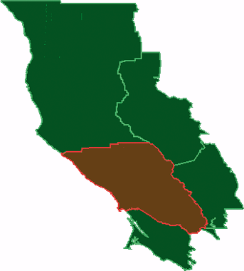
The query in Example 13-5 compares the bounding box of Sonoma County with the shapes of the other bounding boxes. Figure 13-2 shows the shapes and their bounding boxes. Notice how they overlap. When there is an overlap between Sonoma County’s bounding box (shown in red) and the shape of another (shown in green), that other county is selected as a match.

Using bounding boxes this way makes spatial querying much more efficient. PostGIS doesn’t have to do a lot of complex calculations for every vertex or line of every polygon. Instead, it does a rough check using the bounding box rectangles. This uses less memory and is processed much faster.

Figure 13-1. A polygon and its bounding box, shown by the dotted rectangle

Figure 13-2. Sonoma County and surrounding county shapes and bounding boxes

This exercise is supposed to show which counties bordered Sonoma County. If you study Figure 13-2, you will notice that one county isn’t an adjacent neighbor but its bounding box overlaps Sonoma County’s bounding box. This is Yolo County, highlighted in Figure 13-3.

Figure 13-3. Yolo County’s bounding box overlapping Sonoma County’s even though they aren’t adjacent polygons

The && operator is intended to quickly check the general location of shapes. It can’t tell you that two shapes are adjacent, but only if they are close to one another. If two shapes don’t have overlapping bounding boxes, they will not be adjacent. This function is helpful when doing spatial queries because it allows further analysis by PostGIS to focus only on the shapes that might overlap.

To take the query example one step further, the PostGIS Distance() function must be used to determine how close the counties actually are. Example 13-6 is almost identical to Example 13-5 but includes one more WHERE clause.

Example 13-6. Using the distance() function to find adjacent polygons

# SELECT a.county
# FROM countyp020 a,
# countyp020 b
# WHERE b.county = 'Sonoma County'
# AND a.wkb_geometry && b.wkb_geometry
# AND distance(a.wkb_geometry, b.wkb_geometry) = 0;

                       county
----------------------------------------------------
 Sonoma County
 Napa County
 Lake County
 Mendocino County
 Marin County
 Solano County
(6 rows)

The only difference is the last line:

                  AND distance(a.wkb_geometry, b.wkb_geometry) = 0;

The distance function requires two sets of geometry features as parameters. PostGIS calculates the minimum distance between the features in the a.wkb_geometry and b.wkb_geometry columns. If there are any shapes that don’t share the same border as Sonoma County, they are rejected.

Because the && operator is still being used, the distance function is used only to compare the seven features returned by the query in Example 13-5. The resulting set of features are shown on a map in Figure 13-4. Yolo County is no longer part of the result set.

Figure 13-4. The final results show the features selected by the query for counties adjacent to Sonoma County

Planning to visualize query results

If you plan to visualize your results, you can create a view or table with the results of your query. To create a view of the query in Example 13-6, you need to add the CREATE VIEW <view name> AS keywords to the beginning of the SQL statement and wrap your command with parenthesis like this:

# CREATE VIEW mycounties AS
                  (SELECT a.county......=0 );

This view can be accessed just like any table by referring to the name of the view mycounties, instead of the name of a table.

You will also need to make sure to include the geometry results in a column of the query. Earlier examples listed only tabular data, but in order to produce graphics, you need to have a geometry column in your query results. For example, you can modify the SELECT a.county statement in Example 13-6, by adding the geometry column from table a:

# SELECT a.county, a.wkb_geometry

Previous Chapter

13.7. Load Data into the Database

Next Chapter

13.9. Accessing Spatial Data from PostGIS in Other Applications