Giving Directions: The d Attribute

A <path> may be able to draw incredibly complex shapes, but the attribute structure for a <path> element is very simple:

<path d="path-data"/>

The d attribute holds the path instruction set, which can be thought of as a separate coding language within SVG. It consists of a sequence of points and single letter instructions that give the directions for drawing the shape.

Understanding how to draw with SVG <path> elements is therefore a matter of understanding the path-data code.

To allow paths of any complexity, the <path> element lets you specify as many pieces of the path as you need, each using a basic mathematical shape. Straight lines, Bézier curves, and elliptical curves of any length can be specified. Each piece is defined by the type of drawing command, indicated by a letter code, and a series of numerical parameters.

The same path instructions are used outside of SVG. The HTML Canvas2D API (for drawing on a <canvas> element with JavaScript) can now accept path-data strings as input. The same code is also used for paths in Android’s “vector drawables,” which use an XML format that is similar to SVG.

The path instructions are written as a single string of data, and are followed in order. Each path segment starts from the end point of the previous statement; the command letter is followed by coordinates that specify the new end point and—for the more complex curves—the route to get there. Each letter is an abbreviation for a specific command: M, for instance, is short for move-to, while C is cubic curve-to.

There are generally two approaches to rendering the path. In the first approach, path coordinates are given in absolute terms, explicitly describing points in the coordinate system. The single letter commands that control absolute positioning are given as uppercase characters: M, L, A, C, Q, and so on. Changing one point only affects the line segments that directly include that point.

The second approach is to use relative coordinates, indicated by lowercase command letters: m, l, a, c, q, and so on. For relative commands, the coordinates describe the offset from the end of the previous segment, rather than the position relative to the origin of the coordinate system. You can move around a path defined entirely in relative coordinates by changing the first point.

The shorthand custom shapes, <polygon> and <polyline>, only use straight line segments and absolute coordinates. There are no code letters, just a list of points given in the (aptly named) points attribute of each shape:

<polygon points="list of x,y points"/>
<polyline points="list of x,y points"/>

Before getting into the difference between <polygon> and <polyline>, we’ll first go back to <path> (which can substitute for either), and consider what it means to draw a shape from a list of points.

Straight Shooters: The move-to and line-to Commands

The easiest-to-understand path instructions are those that create straight-line shapes. The only numbers you need to include in the directions are the coordinates of the start and end points of the different line segments.

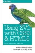
The basic commands you need to know are the M (or m) move-to instruction, and the L (or l) line-to command. For instance, this code creates a path in the shape of a diamond—technically, a rhombus—centered around the point (10,10):

<path d="M3,10 L10,0 L17,10 L10,20 L3,10" />

Filled in red, that looks like this:

The directions in the path data can be read as follows:

• M3,10: move to the point (3,10), meaning the point where x=3 and y=10, without drawing any line;

• L10,0: draw a line from the previous point to the position (10,0);

• L17,10: draw another line from there to (17,10);

• L10,20: draw a third line to (10,20); and finally,

• L3,10: draw a line back to (3,10).

Figure 6-1 shows how the five points in the shape would be positioned if they were marked out on graph paper. The final point exactly overlaps the first.

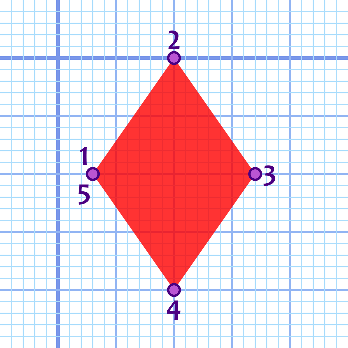
Figure 6-1. A diamond drawn with straight-line path segments

Using relative coordinates, you can define the same path with the following code:

<path d="m3,10 l7,-10 l7,10 l-7,10 l-7,-10"/>

The end result is identical:

In this case, the instructions read:

• m3,10: move 3 units right and 10 units down from the origin;

• l7,-10: draw a straight line starting from the previous point, ending at a new point that is 7 units to the right and 10 units up (that is, 10 units in the negative y direction);

• l7,10: draw another line that ends at a point 7 units further to the right and 10 units back down;

• l-7,10: draw a third line moving back 7 units to the left (the negative x direction) and another 10 units down; and

• l-7,-10: draw a line moving another 7 units left and 10 units up.

To create the same size diamond at a different position, you would only need to change the initial move-to coordinates; everything else is relative to that point.

The relative move-to command in the second snippet may seem equivalent to an absolute M command. Moving x and y units relative to the coordinate system origin is the same as moving to the absolute point (x,y).

However, the move-to commands can also be used partway through the path data. In that case, an m command, with relative coordinates, is not equivalent to an M command with absolute coordinates. Just like with lines, the relative coordinates will then be measured relative to the last end point.

Unlike with lines, the move command is a “pen up” command. The context point is changed, but no line is drawn: no stroke is applied, and the area in between is not enclosed in the fill region. We’ll show an example of move commands in the middle of a path in “Hole-y Orders and Fill Rules”.

Finishing Touches: The close-path Command

The solid fill that was used in Figure 6-1 disguises a problem with paths created only via move-to and line-to commands. If you were to add a stroke with a large stroke width, like in Figure 6-2, you would notice that the left corner, where the path starts and ends, does not match the others.

When a path is drawn, the stroke is open-ended unless it is specifically terminated. What that means is that the stroke will not connect the last point and the first point of a region, even if the two points are the same. The strokes will be drawn as loose ends instead of as corners.

To close a path, use the Z or z close-path command. It tells the browser to connect the end of the path back to the begining, drawing a final straight line from the last point back to the start if necessary. The closing line will have length 0 if the two points coincide.

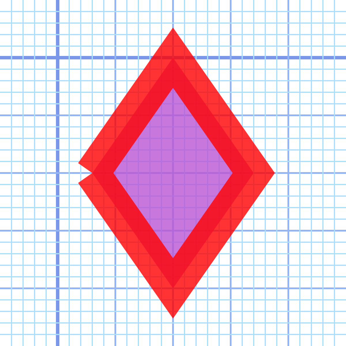
Figure 6-2. An open-path diamond shape, with a thick stroke

The following versions of the diamond each have a closed path; in the second case, it is used to replace the final line-to command, which is preferred:

<path d="M3,10 L10,0 L17,10 L10,20 L3,10 Z" />
<path d="m3,10 l7,-10 l7,10 l-7,10 z"/>

These versions of the path, when stroked using the same styles as before, create the shape shown in Figure 6-3.

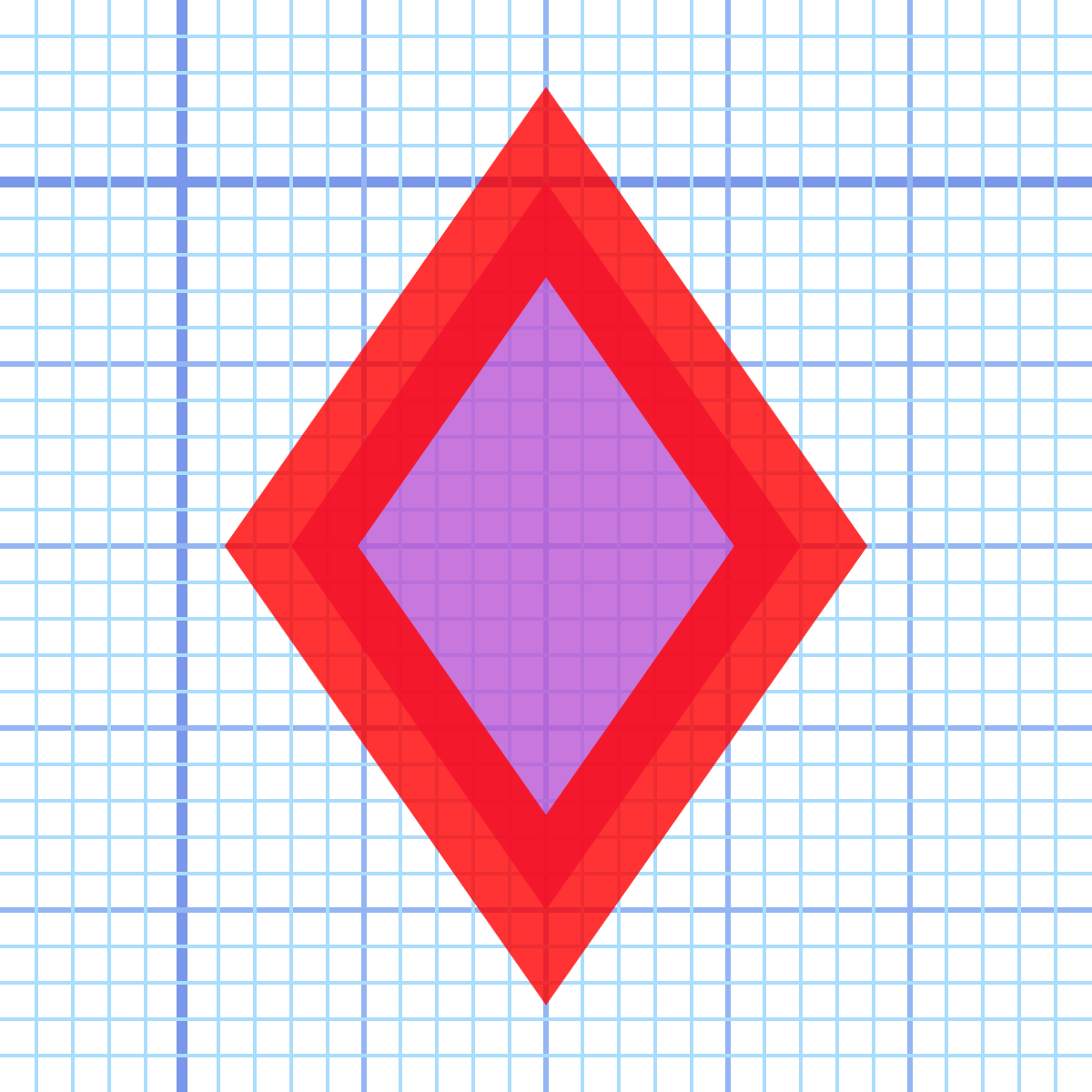
Figure 6-3. A closed-path diamond shape, with a thick stroke

Again, closing a path only affects the stroke, not the fill; the fill region of an open path will always match the closed path, created by drawing a straight line from the final point back to the beginning.

When a path has multiple subpaths created with move-to commands, the close-path command closes the most recent subpath. In other words, it connects to the point defined by the most recent move-to command.

Hole-y Orders and Fill Rules

A useful feature of the “pen-up” move-to command is that it allows you to draw several distinct fill regions in the same path, simply by including additional M or m instructions to start a new section. The different subpaths may be spread across the graphic, visually distinct, but they remain a single element for styling and for interaction with user events.

With multiple subpaths—or even with a single subpath that criss-crosses itself—you can also create “holes” within the path’s fill region. The following version of the diamond includes cut-away regions to suggest light reflecting off a three-dimensional shape, as demonstrated in Figure 6-4.

<path d="M3,10 L10,0 17,10 10,20 Z
         M9,11 L10,18 10,10 15,10 11,9 10,2 10,10 5,10 Z" />

At the default scale, that looks like this:

Figure 6-4 shows how the points are located in the grid. The points are numbered in order, like a connect-the-dots drawing.

Although we haven’t mentioned it so far, the outside diamond shape was intentionally drawn in a clockwise direction. The inner cutout is drawn in a counterclockwise direction. By convention in SVG and other vector graphics languages, the counterclockwise path cancels out the clockwise path, returning the center cutout to the “outside” of the path’s fill region.

If the inside subpath were also clockwise, or if both subpaths were counterclockwise, then it gets more complicated. By default, the inner path would have added to the outside one, and the center region would have still been filled in.

This additive behavior can be controlled with the fill-rule style property. The default value is nonzero; if you switch it to evenodd, cutouts will always be cut out, regardless of the direction of the path.

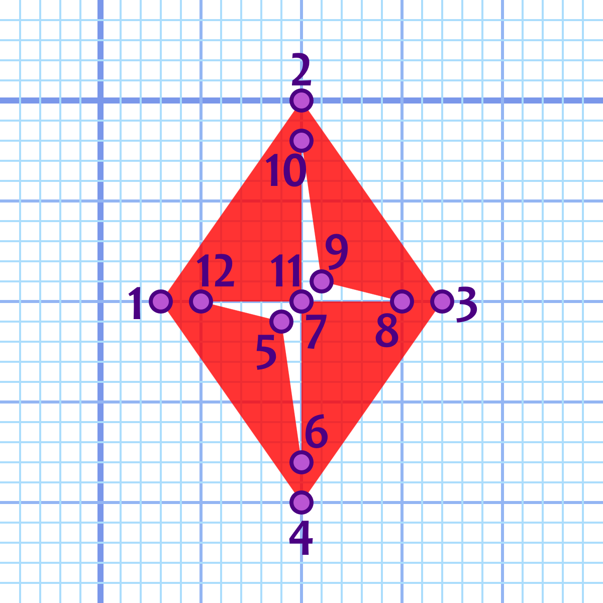
Figure 6-4. A diamond drawn with a cut-out subpath region

Which rule should you use? Which direction should you draw your shapes?

As with most things in programming, it depends.

If both subpaths are drawn in the same direction, you can use fill-rule to control whether they add together (nonzero, the default) or cancel out (evenodd). So you’ll have flexibility later. It’s easier to change a style property than to change your path data.

When a cutout region is drawn in the opposite direction from the main path shape (as in the code for Figure 6-4), it will always be a cutout. So you have predictability.

A fill-rule of evenodd forces the shape to alternate between “inside” and “outside” the path every time it crosses an edge, regardless of whether it is clockwise or counterclockwise. That’s nice and simple, but it means that any overlapping regions are cut out. This can be problematic with complex shapes that have many curves, which might loop around on themselves slightly.

A nonzero fill ensures that these accidental overlaps add together: you have to explictly reverse direction to create a hole.

The fill-rule style property is inherited. It can be declared once for the entire SVG, or it can be defined for individual shapes.

Following the Grid: Horizontal and Vertical Lines

When you define a line with an L (or l) command, you specify both horizontal and vertical coordinates (or offsets, for l). If either the horizontal or vertical position is staying the same, however, there’s a shortcut available.

Precise horizontal and vertical lines can be written concisely with dedicated path commands: H (or h) for horizontal lines, and V (or v) for vertical lines.

These command letters are followed by a single coordinate for the value that is changing. In a horizontal line, the y-value stays the same, so only the x-value is required; in a vertical line, the x-value is constant, so only the y-value is needed.

The following paths therefore both define a 20×10 rectangle with its top-left corner at (10,5) and its bottom-right corner at (30,15). The first path uses absolute coordinates, while the second uses relative offsets:

<path d="M10,5 H30 V15 H0 Z" />
<path d="M10,5 h20 v10 h-20 z" />

Of course, we already have the <rect> element for rectangles. But horizontal and vertical lines show up in many other places. You can create a complete set of gridlines for a chart as a single path with M, H, and V commands. The grids used in the figures in this chapter use a single element for each color and thickness of line:

<path id="axes"
      fill="none" stroke="royalBlue" stroke-width="0.3"
      d="M-5, 0H25 M 0,-5V25"/>
<path id="major-grid"
      fill="none" stroke="cornflowerBlue" stroke-width="0.15"
      d="M-5, 5H25 M 5,-5V25
         M-5,10H25 M10,-5V25
         M-5,15H25 M15,-5V25
         M-5,20H25 M20,-5V25"/>
<!-- And one more, for the minor grid -->

Of course, you can also mix horizontal and vertical with diagonal lines (or curves!) to create all sorts of complex shapes.

The cutout path used for the decorative diamond in Figure 6-4 contains vertical and horizontal lines. After being rewritten to use the shorthand commands, the complete code for the diamond is given in Example 6-1.

<svg xmlns="http://www.w3.org/2000/svg" xml:lang="en"
     height="20px" width="20px">
    <title>Diamond</title>
    <path fill="red"
          d="M3,10 L10,0 17,10 10,20 Z
             M9,11 L10,18 V10 H15 L11,9 10,2 V10 H5 Z" />
</svg>

Using horizontal and vertical commands helps reduce file size, but more importantly: it helps keep your code DRY. It’s easier to change things later if coordinates are not repeated when they don’t have to be.

Of course, reducing file size is a common concern of SVG, and path data was designed with that in mind.

Crunching Characters

This book tries to keep path data legible, by using commas to separate x,y coordinates for a single point and spaces between separate coordinates or separate commands. However, the path syntax is designed to encourage brevity, allowing the path instructions to be condensed considerably:

• Whitespace and commas are interchangeable, and are only required in order to separate numbers that could be mistaken for a single multidigit value.

• The initial zero in a small decimal number can be omitted. This can be combined with the previous rule, so that a line to the point (0.5, 0.7) could be written as L.5.7: you can’t have two decimal places in the same number, so the second . starts a new number.

• The command letter can be omitted when it is the same as the previous path segment, except for multiple move-to commands. Multiple coordinates after a move-to command will be interpreted as line-to commands of the same type (relative or absolute).

The following is a valid equivalent to the diamond shape from Example 6-1. It switches between absolute and relative commands, eliminates separators wherever possible, and uses spaces if a separator is required, without regard to keeping coordinate pairs organized:

<path d="m3 10 7-10 7 10-7 10zM9 11l1 7V10h5l-4-1-1-7v8H5Z"/>

This uses 49 characters to create the same shape that was originally defined in 66 characters plus an indented newline:

<path d="M3,10 L10,0 17,10 10,20 Z
         M9,11 L10,18 V10 H15 L11,9 10,2 V10 H5 Z" />

That’s a savings of more than 25%, which can be significant when you consider that path data often makes up a large portion of SVG file sizes. We highly encourage you to use SVG optimizer tools to condense very large path data strings. But for handwriting code—and reading it later—we’ll be sticking with the “pretty” versions.

Short and Sweet Shapes: Polygons and Polylines

There’s another, more legible way to simplify straight-line paths: use a <polygon> or <polyline> element.

Both of these elements allow you to create straight-line shapes simply by giving a list of the corner points in the points attribute. The points in a <polyline> create an open path when stroked; for <polygon>, the shape is closed from the last point back to the first.

The coordinates are always absolute, and can be separated by whitespace or commas, in whichever organization makes sense to you. Here is the basic diamond once again, as a four-point <polygon>:

<polygon points="3,10 10,0 17,10 10,20" />

There are a number of features of SVG that (in SVG 1.1) are only available for <path> elements, and not other shapes. This includes text on a path (which we’ll introduce in Chapter 7) and the JavaScript functions for accessing the length of a path (which we’ll discuss in Chapter 13).

If need be, you can always convert the simple list of points for <polygon> to a <path> data attribute by inserting an M at the beginning and a Z at the end. For a <polyline>, skip the Z to keep the path open-ended.

Another reason to convert polygons to paths is to combine multiple shapes into subpaths of a single complex shape. Polygons and polylines can only have a single, continuous shape.

Even without distinct subpaths, polygons can have “holes” created by criss-crossing edges. Because the edges will all be part of the same continuous shape, the winding order won’t change, so the fill rules are simpler than for multipart paths. The overlapping sections will only be treated as holes if you set fill-rule: evenodd.

The remaining sections of the chapter focus on curved paths, which means we’re focusing exclusively on the <path> element, not on <polygon> or <polyline>.

Curve Balls: The Quadratic Bézier Command

Anyone who has ever put together a connect-the-dots picture knows that straight lines, while useful for getting a general feel for a given shape, are at best a loose approximation of the real world. For a graphics language, the ability to generate curved segments between points is essential.

SVG paths use three types of curves: quadratic Bézier curves, cubic Bézier curves, and elliptical curves. Bézier curves are also available with shorthand smooth-curve commands, and each curve command can be expressed in absolute or relative coordinates. All these options can be a little daunting on first impression, but understanding this breakdown can make the selection of the best curve forms easier.

Bézier curves rely on two convenient truths:

• You can express close approximations to most continuous curves by using a series of quadratic or cubic equations (equations where the y position is related to x² or x³, respectively) connected together in a spline, such that the curve flows smoothly from one segment to the next.

  It’s not always a perfect approximation—in equations where more complex mathematical relationships predominate, finding an exact match with a Bézier equation can be difficult at best—but you can always improve the approximation by using a greater number of shorter curve segments, smoothed together.

• You can calculate quadratic and cubic curves over a finite area as a weighted average of multiple x,y points: end points for the curve segment and control points defining its shape.

  Computers can calculate these weighted averages much more efficiently than they can squares or cubes, and many times faster than they can calculate more complicated mathematical relationships.

What does “a weighted average of multiple x,y points” mean? Consider Figure 6-5, which is an exact repeat of Figure 5-2 from Chapter 5.

The start points of each line in the top right of the graphic are each a percentage of the distance between (0,0) and the point (10cm, 0); the end points of each line are each positioned at a matching percentage of the distance between (10cm, 0) and (10cm, 10cm). This is a direct result of how the lines were created in the JavaScript loops.

Less obvious is that the same percentages apply to the apparent curved line created by the overlapping, intersecting lines. The first line, the one whose start and end points are weighted entirely to the initial positions, sketches out the very beginning of the curve. The second line, which starts and ends 10% of the way along the square’s edges, intersects that curve at 10% of its (the line’s) length. And so on for the rest of the lines: the middle line, which spans from (5cm, 0) to (10cm, 5cm), crosses the curve at its halfway point; the line from (8cm, 0) to (10cm, 8cm) crosses the curve 80% of the way to its end point.

The apparent curve created by those intersecting straight lines can be directly drawn as a quadratic Bézier curve. A quadratic Bézier requires three points: the start point, an end point, and a single control point between them that establishes the farthest extent of the mesh envelope (aka the string art). For the curves created by the lines in Figure 6-5, the start and end points are (0,0) and (10cm, 10cm); the control points are (10cm, 0) for the top half of the curve and (0, 10cm) for the lower half.

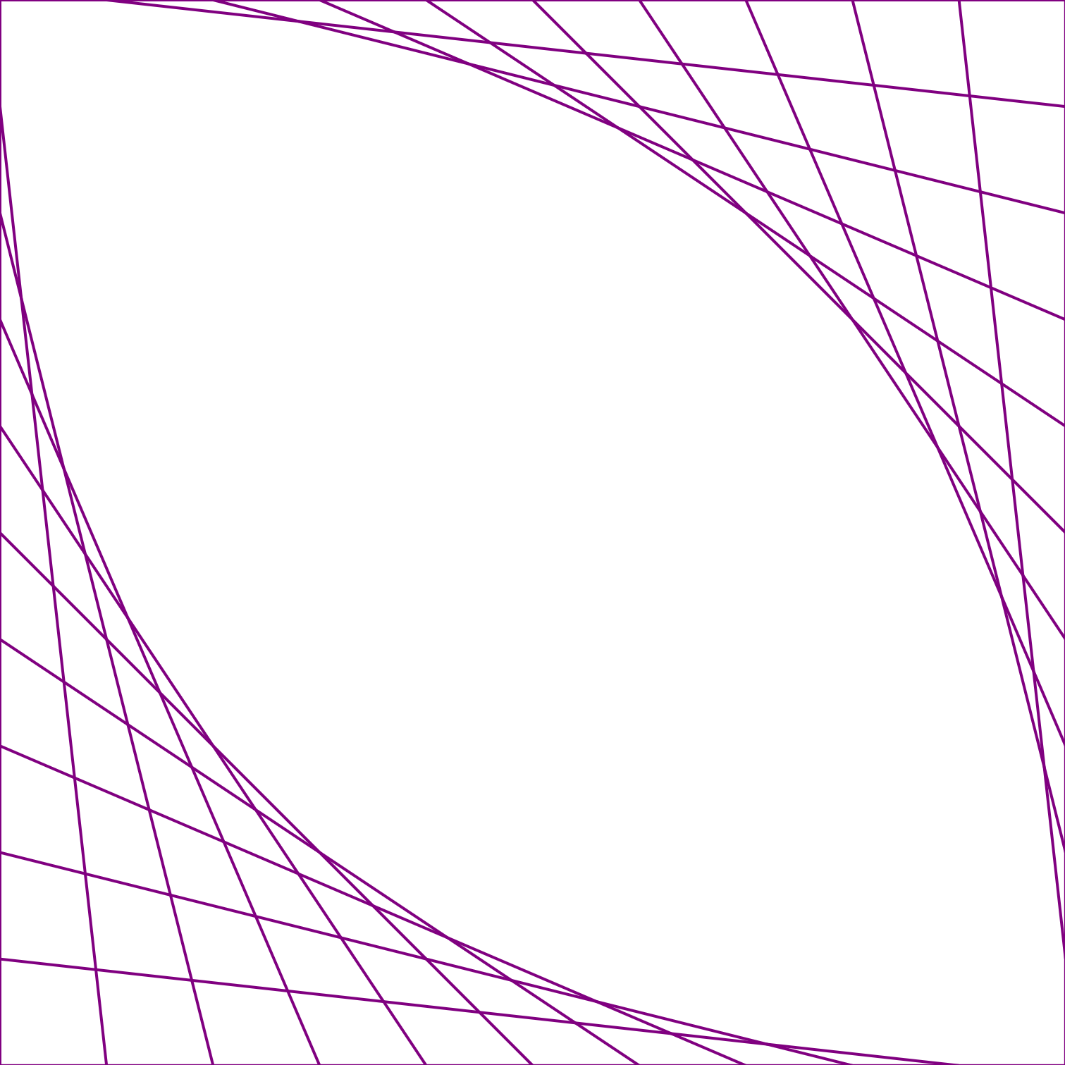
Figure 6-5. String art “curves” created from SVG lines

Figure 6-6 adds those two Bézier curves, as two halves of a filled-in shape, to the SVG. As you can see, the lines perfectly brush the edges of the curved shape.

In SVG path notation, the command letter for quadratic curves is Q (or q for relative coordinates). As with all path commands, the start point is taken from the end point of the previous command in the path. That means that a Q is followed by two pairs of x,y coordinates: the first pair of numbers describes the control point, and the second pair defines the end point.

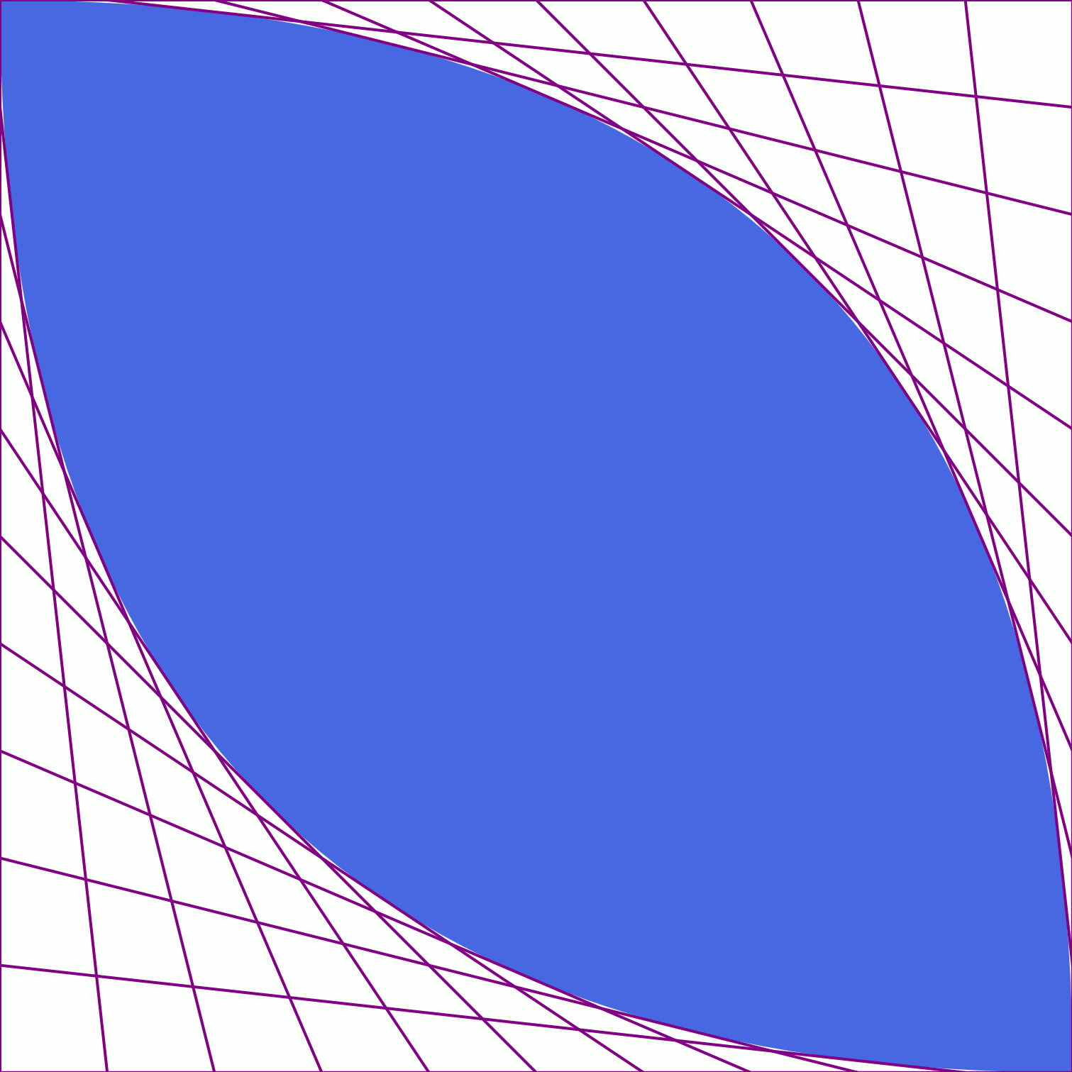
Figure 6-6. A quadratic Bézier path, and the string art mesh that encloses it

Curves shaped like those in Figure 6-6 would be written as follows, in a 10×10 coordinate system:

<path d="M0,0 Q 10, 0 10,10
              Q  0,10  0,0 Z" />

It starts from the top-left (0,0) point, moves clockwise around the upper curve to the bottom corner, then moves back up along the bottom curve.

In relative coordinates, the curve would be:

<path d="m0,0 q 10,0  10,10
              q-10,0 -10,-10 z" />

Since the path starts from (0,0), the numbers in the first segment haven’t changed; the numbers in the second segment are all relative to the (10,10) point from the end of the first curve.

There’s just one more complication. As we briefly mentioned earlier, you cannot use units like cm in path data coordinates; you must use user coordinate numbers. The preceding paths draw shapes 10px tall and wide, not 10cm.

In Chapter 8 we’ll discuss how you can use nested coordinate systems to scale a specific number of user coordinates to exactly match a chosen length. For now, we’ll take advantage of the fact that user coordinates are equivalent to CSS px units, and all modern browsers scale real-world units so that there are 96px per in. Since there are 2.54cm per inch—in the real world or in your browser—this means that 10cm is (10*96/2.54) user units, or approximately 377.95 units.

The following path therefore draws the two quadratic curves in Figure 6-6:

<path d="M0,0 Q377.95,0 377.95,377.95
              Q0,377.95 0,0 Z"
      fill="royalBlue" />

Smooth Operators: The Smooth Quadratic Command

The two quadratic curves used in Figure 6-6 meet at sharp points. However, earlier we mentioned that you can create continuous curves by connecting multiple Bézier curves smoothly.

What makes a smooth connection between curves? A smooth curve does not have any sudden changes in direction. In order to connect two curved path segments smoothly, the direction of the curve as it reaches the end of the first segment must exactly match the direction of the curve as it begins the next segment.

Take a look at Figure 6-6 again. The direction of the start of each curve segment is the direction of the line from the start point to the control point. The direction of the end of each segment matches the line from the control point to the end point. Those lines are tangent to the start and end of the curve. Line them up so one tangent is a continuation of the other, and your curve will look continuous too.

SVG has a shortcut to make smooth curves easier. The T (or t) command creates a quadratic curve that smoothly extends the previous Bézier curve segment. The control point is calculated automatically, based on the control point from the previous segment; the new control point is positioned the same distance from its start point (the previous segment’s end point) as the other control point is, but in a straight line on the opposite side.

Figure 6-7 shows what that looks like. The distance from the control point of the first segment to the mid-point is 3 units right and 5 units down. The reflected control point for the next segment is therefore an additional 3 units right and 5 units down. Note that while the control points are reflected, the final shape of the curve is not a mirror reflection. (It could be, but only if the other points were all arranged symmetrically, too.)

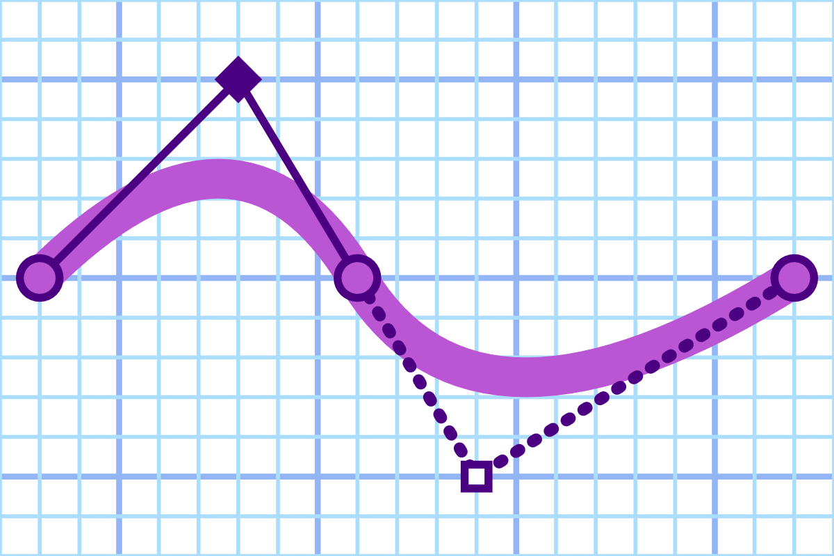
Figure 6-7. A curve made of two quadratic segments, with the control point reflected from the first segment to the second

If the curve segment prior to a T command wasn’t a quadratic Bézier (smooth or otherwise), the control point for the new segment defaults to its start point. This effectively turns the T segment into a straight line, and turns your smooth connection into a sharp corner.

The smooth curve command is not the only way to smoothly connect Bézier curves. If the second curve should be much deeper or shallower than the previous one, you may need to move the control point to be closer or farther away from the end point, without changing the direction of the tangent line.

To do this, make sure the slope of the tangent lines remains the same: the ratio of the change in y-values to the change in x-values. You can also use this calculation to create a curve that smoothly extends from a straight line; the line is its own tangent.

Example 6-2 uses quadratic curves to create a heart icon to match the diamond, with a mix of manual and shorthand smooth connections. The end result should look like this:

<svg xmlns="http://www.w3.org/2000/svg" xml:lang="en"
     height="20px" width="20px">
    <title>Heart</title>
    <path fill="red"
          d="M 10,6
             Q 10,0 15,0
             T 20,6
             Q 20,10 15,14
             T 10,20
             Q 10,18 5,14
             T 0,6
             Q 0,0 5,0
             T 10,6
             Z" />
</svg>

Figure 6-8 shows the shape, scaled up on the grid. The connect-the-dots numbers have been omitted so we can instead emphasize the positions of the control points. Explicit control points (the ones specified in the code) are marked with solid lines and dark markers; the reflected control points are shown with dotted lines and white square markers.

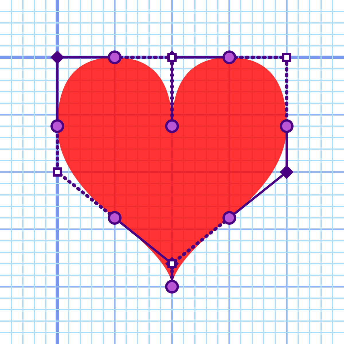
Figure 6-8. A heart drawn with quadratic Bézier curves, showing the control points

The first half of the path directions can be read as follows:

• M 10,6 starts the path at the dimple of the heart, horizontally centered in the 20px width.

• Q 10,0 15,0 creates the first curve segment, tracing the shape of the heart in a clockwise direction. The control point is (10,0) and the end point is (15,0), at the top of the right lobe of the heart.

• T 20,6 creates a smooth quadratic curve to the far rightmost edge of the heart. The missing control point can be calculated from the previous segment: the tangent line from (10,0) to (15,0) moved 5 units in the x-direction and 0 units vertically; you locate the new control point by repeating that vector, from (15,0) to (20,0).

• Q 20,10 15,14 manually creates a smooth connection to the next quadratic curve. The ending tangent of the previous segment, from (20,0) to (20,6), was perfectly vertical, so it was easy to position the new control point, (20,10), along the same line. Using that control point, the path segment curves inward to (15,14).

• T 10,20 smoothly extends the curve, inflecting it back downward to the bottom point of the heart shape. The line from the previous control point (20,10) to the start/end point (15,14) was equal to –5 x units and +4 y units, so the automatically calculated control point will be that same offset again, from (15,14) to (10,18).

The next segment is not a smooth continuation of the curve; the bottom of the heart is a sharp point. The rest of the heart is symmetrical to the part drawn so far, reflected around the line y=10.

This type of symmetry, it turns out, doesn’t make very good use of the automatically calculated control points; in order to recreate the same curves on the other side of the heart, you need to know the control points from the first half. The Q 10,18 5,14 segment is the reflection of the T 10,20 segment, but in this case the (10,18) control point needs to be explicitly stated.

With quadratic curves, eight curve segments are required to draw the heart. Each segment can only curve in a single direction, and the start and end points for each segment must be chosen so that a single control point can define both the tangent line that starts the curve and the tangent line that ends it.

To gain more flexibility—to allow the ending tangent of the curve segment to be defined independently from the starting tangent—you need to use cubic curves. But rather than redrawing the heart, the next section uses cubic curves to add a spade to our set of card suit icons.

Wave Motion: The Cubic Bézier Commands

A quadratic Bézier curve is a parabola—useful for creating gentle curves that have a single bend. A cubic Bézier curve, on the other hand, is much more flexible.

A cubic curve is defined by two control points. The first defines the tangent line from the start point, and the second defines the tangent line to the end point.

If the tangent lines point in opposite directions, a cubic curve segment may have two bends, curving like a letter S in opposite directions. With other control points, the segment may look more like a letter C. A cubic curve may also look not that different from a quadratic curve, with only one gentle bend—or no bend at all, if the two control points fall directly on the line between the start and end points.

Most drawing applications primarily use cubic Bézier curves because they are more flexible than quadratic ones.

Figure 6-9 shows how this flexibility can create curves that no longer feel neat and geometric. The curve consists of two cubic segments, which are smoothly joined with reflecting control points in the middle. But the control points on the ends angle out in completely unrelated directions.

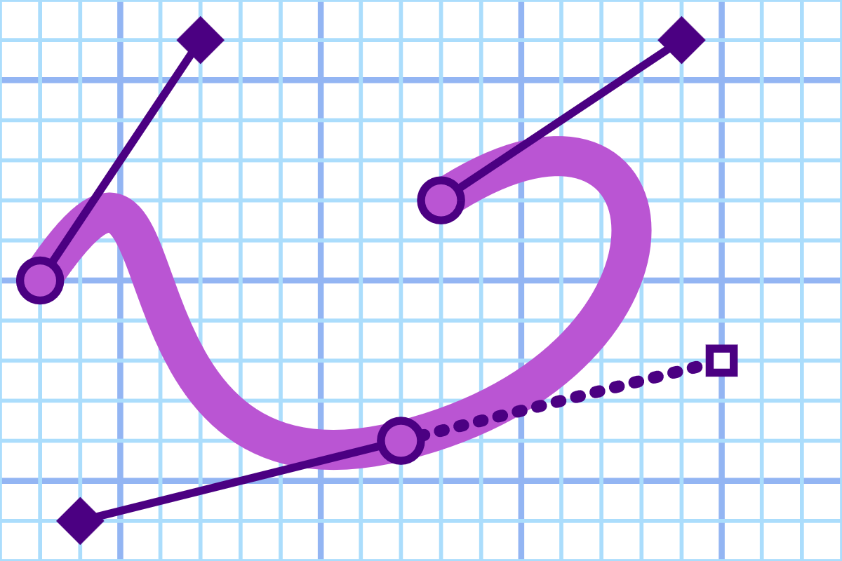
Figure 6-9. A curve made from two cubic Bézier segments, showing the control points

In the path directions, cubic curves use the letter C (or c) followed by three sets of coordinates, for the first and second control points and the end point. As always, the start point is taken from the end of the previous command.

Smooth cubic Béziers curves can be used in a similar manner to smooth quadratics. The command letter is S (or s) and it is followed by two sets of coordinates, for the second control point and the end point. The curve in Figure 6-9 uses the following code:

<path d="M 3,10
         C 7,4  4,16 12,14
         S     19,4  13,8 " />

The first control point for the smooth segment is calculated automatically.

As with the quadratic smooth curve command, the smooth shorthand only works in certain situations. If you use an S command after a segment that wasn’t a cubic Bézier—including after a quadratic Bézier—the automatically calculated control point will default to the curve’s start point. This doesn’t convert the curve to a straight line (as it did for T), since the second control point will still introduce a bend. But it will destroy the smoothness of the connection.

Example 6-3 continues our series of card suit icons, drawing the following spade shape using cubic Bézier curves:

<svg xmlns="http://www.w3.org/2000/svg" xml:lang="en"
     height="20px" width="20px">
    <title>Spade</title>
    <path fill="black"
          d="M 9,15
             C 9,20 0,21 0,16
             S 6,9 10,0
             C 14,9 20,11 20,16
             S 11,20 11,15
             Q 11,20 13,20
             H 7
             Q 9,20 9,15 Z" />
</svg>

Figure 6-10 shows the scaled-up result with the points marked out on the grid. Again, the solid lines and diamonds mark the explicitly defined control points, while the dotted line and white squares mark the reflected control points. The control points for the cubic and quadratic curves overlap at the stem.

The directions can be read as follows:

• M 9,15 positions the start of the path at the point where the left lobe connects with the stem. As usual, the path will progress clockwise around the shape—direction might not matter if you’re not creating cutouts, but it’s a good habit to always use clockwise shapes.

• C 9,20 0,21 0,16 draws the entire lower curve of the left lobe. The initial tangent line points directly downward, from (9,15) to (9,20), while the ending tangent line points directly upward, from (0,21) to the end point of (0,16).

• S 6,9 10,0 creates a smooth continuation of the curve, ending with a tangent line from (6,9) to the center point of (10,0).

• C 14,9 20,11 20,16 creates the symmetrical curve: the initial (14,9) control point is the reflection of the (6,9) point from the previous curve, while the second control point (20,11) is the reflection of the point that had been automatically calculated in the previous segment. The (20,16) end point matches the (0,16) point from the initial cubic curve.

• S 11,20 11,15 draws the right lower lobe, reflecting the shape of the left lower lobe.

• Q 11,20 13,20 creates a quadratic curve for the right side of the stem.

• H 7 draws the horizontal line across the bottom of the stem.

• Q 9,20 9,15 Z draws the matching quadratic curve for the opposite edge of the stem, and closes off the path.

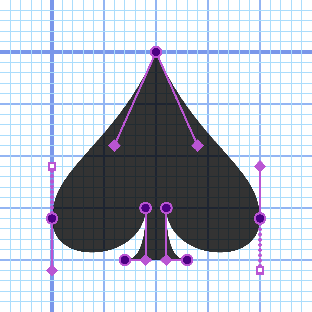
Figure 6-10. A spade drawn with cubic Bézier curves, showing the control points

Using cubic curves, each lobe of the spade was drawn with two path segments, compared to the four quadratic segments required for each lobe of the heart.

Building the Arcs

In general, cubic Bézier curves can be used to encode nearly any type of shape you might want to draw. However, as mentioned previously, Bézier curves will never perfectly match shapes based on mathematical relationships other than quadratic or cubic functions. You can never draw a perfect circle or ellipse with a Bézier curve. Because perfect circular arcs are expected in many diagrams, SVG includes a separate command specifically for them.

The final path command in the SVG toolbox is the arc segment (A or a), which creates a circular arc between two points. This is useful for creating circular arcs for pie charts and elliptical arcs for…um, flattened pie charts? It also allows you to create the asymmetrical rounded rectangles that we alluded to in Chapter 5.

The syntax for the arc command is a little more complex than for the Bézier segments. The required parameters are as follows:

A rx ry x-axis-rotation large-arc-flag sweep-flag x y

The x and y values at the end of the command are the coordinates of the end point of the arc. These are the only values that differ between absolute (A) and relative (a) arc commands.

The rx and ry parameters specify the horizontal and vertical radii lengths of the ellipse from which the arc will be extracted. There’s no separate syntax for circular arcs; just set rx and ry to the same value.

The next number (x-axis-rotation) allows you to rotate the x-axis of the ellipse relative to the x-axis of the coordinate system. The rotation number is interpreted in degrees; positive values are clockwise rotation, and negative values are counterclockwise. For circular arcs, this value is usually 0; rotating a circle has no visible effect on its shape.

The next two parameters tend to confuse people. To fully understand the large-arc-flag and sweep-flag, it may help to try drawing arcs by hand.

Grab your coffee mug, get a coin out of your pocket, or use a jar, tube, or anything else circular—or elliptical, if you can find an ellipse! Your circular/elliptical design aid, whatever it is, has a fixed radius in both directions. If it’s elliptical, try to hold it at a fixed angle, too. Try out this exercise:

1. Take a piece of paper, and mark two points on it for your arc’s start point and end point. Don’t make them too far apart.

2. Set your coin/coffee mug down on the paper and adjust it until it touches both points.

3. Trace a curve around your circular object to connect the points.

4. Then, trace another curve around the other side of your circle.

5. Take your circle and shift it so that its center point is on the opposite side of the straight line between your start and end points. Readjust it so that it just touches the start and end points.

6. Trace around the circle to connect up the points again, from both directions.

7. Remove your coin/coffee mug. You should have a drawing that looks vaguely like Figure 6-11.

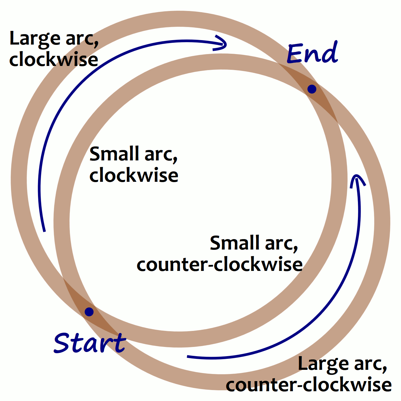
Figure 6-11. The many ways to connect two points with a coffee mug stain

Each of the four arcs in Figure 6-11 has been labeled by (a) whether it goes around the longer route (large arc) or the shorter route (small arc), and (b) whether the path from start to end goes around the circle clockwise or counterclockwise. These are the parameters that you specify with the large-arc-flag and sweep-flag. These parameters are flags, meaning that they are “true” (value 1) if the arc should have that property, and “false” (value 0) otherwise.

The sweep-flag could be called the clockwise-flag, but that would only confuse things once we start transforming the coordinate system. Transformations can create mirror-reflected situations where clockwise isn’t clockwise anymore.

If this seems overly confusing, it is. The elliptical arc is one of those commands that gives up in legibility more than what it gains in flexibility. In order to integrate arcs into continuous paths, they need to be defined by precise start and end points, which isn’t how arcs are usually defined in geometry.

The code to draw Figure 6-11 is provided in the online supplementary material. The four arcs are all the same except for the 0 or 1 values in the flag parameters:

<path d="M100,350 A180,180 0 1 1 350,100" />
<path d="M100,350 A180,180 0 0 1 350,100" />
<path d="M100,350 A180,180 0 0 0 350,100" />
<path d="M100,350 A180,180 0 1 0 350,100" />

Make sure you know which one is which!

Using arcs, we can complete the card suit icon set. The code for this club icon is given in Example 6-4:

<svg xmlns="http://www.w3.org/2000/svg" xml:lang="en"
     height="20px" width="20px">
    <title>Club</title>
    <path fill="black"
          d="M 9,15.5
             A 5,5 0 1 1 5.5,7.5
             A 5,5 0 1 1 14.5,7.5
             A 5,5 0 1 1 11,15.5
             Q 11,20 13,20
             H 7
             Q 9,20 9,15.5 Z" />
</svg>

All three arcs are “large,” and the entire shape is drawn in a clockwise direction, so both flags are set to 1 for each A command. The stem is the same as for the spade in Example 6-3.

Figure 6-12 shows the enlarged figure, including the complete circles from which the arcs are extracted.

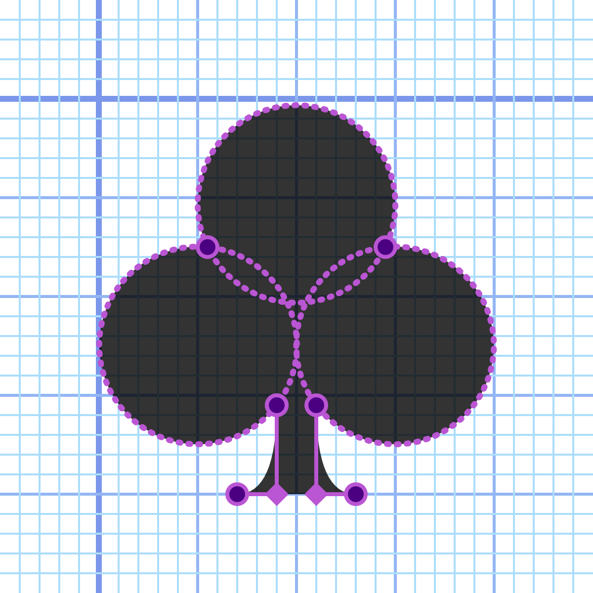
Figure 6-12. A club drawn with path arc commands, showing the underlying geometry

Summary: Custom Shapes

The core concept of SVG (and vector graphics, in general) is that drawings can be described through a set of precise mathematical instructions. With the exception of the few common shape elements described in Chapter 5, most SVG shapes are drawn point by point, using <polygon>, <polyline>, or the infinitely flexible <path>.

While <polygon> and <polyline> elements can be described by a simple list of points, the <path> uses its own language to describe what type of line to draw and how.

Drawing a shape is the first step in creating a piece of artwork, and the tools that SVG provides here are extremely robust. The next step is to be able to position and manipulate those shapes within the vector coordinate system.

The basic shapes <line>, <rect>, <circle>, and <ellipse>, while limited in geometry, are incredibly flexible in size because each geometric attribute can be set independently with user coordinates, units, or percentages. In contrast, <path>, <polygon>, and <polyline> allow complete customization of the shape, but all the points must be defined relative to the user coordinate system. To create flexibility in their position and size, you need to manipulate the coordinate system directly, something we’ll explore in Part III.

Before we get there, however, we have one final set of SVG shapes to discuss: letters! And numbers! And emoji! In other words, text—the topic of Chapter 7.