Chapter 12

Tables

12.1 Introduction

In the last few chapters, we’ve dealt primarily with manipulating numbers and performing logical operations. Another common task that microprocessors usually perform is searching for data in memory from a list of elements, where an element could be sampled data stored from sensors or analog-to-digital converters (ADCs), or even data in a buffer that is to be transmitted to an external device. In the last 10 years, research into sorting and search techniques have, in part, been driven by the ubiquity of the Internet, and while the theory behind new algorithms could easily fill several books, we can still examine some simple and very practical methods of searching. Lookup tables are sometimes efficient replacements for more elaborate routines when functions like log(x) and tan(x) are needed; the disadvantage is that you often trade memory usage and precision for speed. Before we examine subroutines, it’s worth taking a short look at some of the basic uses of tables and lists, for both integer and floating-point algorithms, as this will ease us into the topic of queues and stacks.

12.2 Integer Lookup Tables

Consider a list of elements ordered in memory starting at a given address. Suppose that each element in the list is a word in length, as shown in Figure 12.1. Addressing a particular element in the list becomes quite easy, since the ARM addressing modes allow pre-indexed addressing with an offset. More precisely, if the starting address were held in register r5, then a given element could either be addressed by putting an offset in another register, or the element number can be used to generate an offset by scaling. The third element in the list could be accessed using either

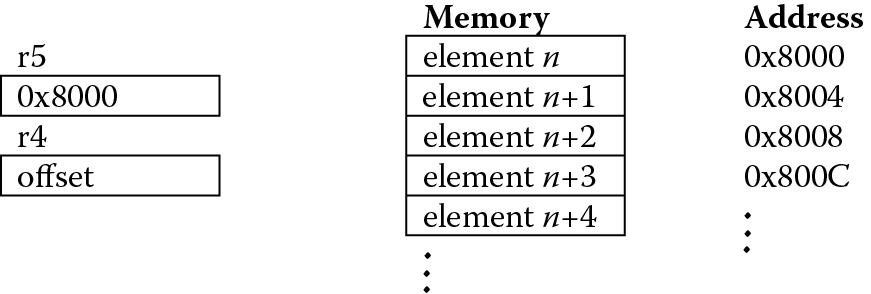
LDR r6, [r5, r4]

or

LDR r6, [r5, r4, LSL #2]

where register r4 would contain the value 8, the actual offset, in the first case, or 2, one less than the element number, in the second case (for our discussion, the first element is number zero). The latter addressing mode accounts for the size of the data by scaling the element number by 4.

Certainly the same concepts apply if the elements are halfwords, only now the load instructions would be

LDRH r6, [r4, r5]

and

LDRH r6, [r4, r5, LSL #1]

Example 12.1

Many control and audio applications require computing transcendental functions, such as log(x), tan(x), and sin(x). An easy way to compute the sine of an angle is to use a lookup table. There are obvious limits to the precision available with such a method, and if greater precision is required, there are very good routines for computing these types of functions, such as those by Symes (Sloss, Symes, and Wright 2004). However, a lookup table can return a value in Q31 notation for integer values of the angle between 0 and 360 degrees, and the implementation is not at all difficult.

To begin, it’s necessary to create a table of sine values for angles between 0 and 90 degrees using Q notation. A short C program can generate these values very quickly, and if you throw in a little formatting at the end, it will save you the time of having to add assembler directives. The C code* below will do the trick:

#include <stdio.h > 

#include <string.h > 

#include <math.h > 

main()

{

	int i;

	int index = 0;

	signed int j[92];

	float sin_val;

	FILE *fp;

	if ((fp = fopen(“sindata.txt”,”w”)) = =NULL)

	{

		printf(“File could not be opened for writing\n”);

		exit(1);

	}

	for (i = 0; i < =90; i + +){

		/* convert to radians */

		sin_val = sin(M_PI*i/180.0);

		/* convert to Q31 notation */

		j[i] = sin_val * (2147483648);

		}

	for (i = 1; i < =23; i + +){

		fprintf(fp,”DCD “);

		fprintf(fp,”0x%x,”,j[index]);

		fprintf(fp,”0x%x,”,j[index + 1]);

		fprintf(fp,”0x%x,”,j[index + 2]);

		fprintf(fp,”0x%x”,j[index + 3]);

		fprintf(fp,”\n”);

		index += 4;

		}

	fclose(fp);

}

It’s important to note that while generic C code like this will produce accurate values for angles between 0 and 89 degrees, it’s still necessary to manually change the value for 90 degrees to 0x7FFFFFFF, since you cannot represent the number 1 in Q31 notation (convince yourself of this). Therefore, we will just use the largest value possible in a fractional notation like this. The next step is to take the table generated and put this into an assembly program, such as the ones shown below for the ARM7TDMI and the Cortex-M4. While this is clearly not optimized code, it serves to illustrate several points.

; Example for the ARM7TDMI

	AREA SINETABLE, CODE

	ENTRY

; Registers used:

; r0 = return value in Q31 notation

; r1 = sin argument (in degrees, from 0 to 360)

; r2 = temp

; r4 = starting address of sine table

; r7 = copy of argument

main

	MOV	r7,r1	; make a copy of the argument

	LDR	r2, = 270	; constant won’t fit into rotation scheme

	ADR	r4, sin_data	; load address of sin table

	CMP	r1, #90	; determine quadrant

	BLE	retvalue	; first quadrant?

	CMP	r1, #180

	RSBLE	r1,r1,#180	; second quadrant?

	BLE	retvalue

	CMP	r1, r2

	SUBLE	r1, r1, #180	; third quadrant?

	BLE	retvalue

	RSB	r1, r1, #360	; otherwise, fourth

retvalue

	; get sin value from table

	LDR	r0, [r4, r1, LSL #2]

	CMP	r7, #180	; do we return a neg value?

	RSBGT	r0, r0, #0	; negate the value if so

done	B	done

ALIGN

sin_data

		DCD 0x00000000,0x023BE164,0x04779630,0x06B2F1D8

		DCD 0x08EDC7B0,0x0B27EB50,0x0D613050,0x0F996A30

		DCD 0x11D06CA0,0x14060B80,0x163A1A80,0x186C6DE0

		DCD 0x1A9CD9C0,0x1CCB3220,0x1EF74C00,0x2120FB80

		DCD 0x234815C0,0x256C6F80,0x278DDE80,0x29AC3780

		DCD 0x2BC750C0,0x2DDF0040,0x2FF31BC0,0x32037A40

		DCD 0x340FF240,0x36185B00,0x381C8BC0,0x3A1C5C80

		DCD 0x3C17A500,0x3E0E3DC0,0x40000000,0x41ECC480

		DCD 0x43D46500,0x45B6BB80,0x4793A200,0x496AF400

		DCD 0x4B3C8C00,0x4D084600,0x4ECDFF00,0x508D9200

		DCD 0x5246DD00,0x53F9BE00,0x55A61280,0x574BB900

		DCD 0x58EA9100,0x5A827980,0x5C135380,0x5D9CFF80

		DCD 0x5F1F5F00,0x609A5280,0x620DBE80,0x63798500

		DCD 0x64DD8900,0x6639B080,0x678DDE80,0x68D9F980

		DCD 0x6A1DE700,0x6B598F00,0x6C8CD700,0x6DB7A880

		DCD 0x6ED9EC00,0x6FF38A00,0x71046D00,0x720C8080

		DCD 0x730BAF00,0x7401E500,0x74EF0F00,0x75D31A80

		DCD 0x76ADF600,0x777F9000,0x7847D900,0x7906C080

		DCD 0x79BC3880,0x7A683200,0x7B0A9F80,0x7BA37500

		DCD 0x7C32A680,0x7CB82880,0x7D33F100,0x7DA5F580

		DCD 0x7E0E2E00,0x7E6C9280,0x7EC11A80,0x7F0BC080

		DCD 0x7F4C7E80,0x7F834F00,0x7FB02E00,0x7FD31780

		DCD 0x7FEC0A00,0x7FFB0280,0x7FFFFFFF

		END

; Program for the Cortex-M4

		MOV	r7,r1	; make a copy of the argument

		LDR	r2, = 270 	; constant won’t fit into rotation scheme

		ADR	r4, sin_data	; load address of sin table

		CMP	r1, #90	; determine quadrant

		BLE	retvalue	; first quadrant?

		CMP	r1, #180

		ITT	LE

		RSBLE	r1,r1,#180	; second quadrant?

		BLE	retvalue

		CMP	r1, r2

		ITT	LE

		SUBLE	r1, r1, #180	; third quadrant?

		BLE	retvalue

		RSB	r1, r1, #360	; otherwise, fourth

retvalue

		; get sin value from table

		LDR	r0, [r4, r1, LSL #2]

		CMP	r7, #180	; do we return a neg value?

		IT	GT

		RSBGT	r0, r0, #0	; negate the value if so

done		B	done

		ALIGN

sin_data

		DCD 0x00000000,0x023BE164,0x04779630,0x06B2F1D8

		DCD 0x08EDC7B0,0x0B27EB50,0x0D613050,0x0F996A30

		DCD 0x11D06CA0,0x14060B80,0x163A1A80,0x186C6DE0

		DCD 0x1A9CD9C0,0x1CCB3220,0x1EF74C00,0x2120FB80

		DCD 0x234815C0,0x256C6F80,0x278DDE80,0x29AC3780

		DCD 0x2BC750C0,0x2DDF0040,0x2FF31BC0,0x32037A40

		DCD 0x340FF240,0x36185B00,0x381C8BC0,0x3A1C5C80

		DCD 0x3C17A500,0x3E0E3DC0,0x40000000,0x41ECC480

		DCD 0x43D46500,0x45B6BB80,0x4793A200,0x496AF400

		DCD 0x4B3C8C00,0x4D084600,0x4ECDFF00,0x508D9200

		DCD 0x5246DD00,0x53F9BE00,0x55A61280,0x574BB900

		DCD 0x58EA9100,0x5A827980,0x5C135380,0x5D9CFF80

		DCD 0x5F1F5F00,0x609A5280,0x620DBE80,0x63798500

		DCD 0x64DD8900,0x6639B080,0x678DDE80,0x68D9F980

		DCD 0x6A1DE700,0x6B598F00,0x6C8CD700,0x6DB7A880

		DCD 0x6ED9EC00,0x6FF38A00,0x71046D00,0x720C8080

		DCD 0x730BAF00,0x7401E500,0x74EF0F00,0x75D31A80

		DCD 0x76ADF600,0x777F9000,0x7847D900,0x7906C080

		DCD 0x79BC3880,0x7A683200,0x7B0A9F80,0x7BA37500

		DCD 0x7C32A680,0x7CB82880,0x7D33F100,0x7DA5F580

		DCD 0x7E0E2E00,0x7E6C9280,0x7EC11A80,0x7F0BC080

		DCD 0x7F4C7E80,0x7F834F00,0x7FB02E00,0x7FD31780

		DCD 0x7FEC0A00,0x7FFB0280,0x7FFFFFFF

The first task of the program is to determine in which quadrant the argument lies. Since

sin(x) = sin(180° – x)

and

sin(x − 180°) = −sin(x)

sin(360° − x) = −sin(x)

we can simply compute the value of sine for the argument’s reference angle in the first quadrant and then negate the result as necessary. The first part of the assembly program compares the angle to 90 degrees, then 180 degrees, then 270 degrees. If it’s over 270 degrees, then by default it must be in the fourth quadrant. The reference angle is also calculated to use as a part of the index into the table, using SUB or RSB as necessary. For values that lie in either the third or fourth quadrant, the final result will need to be negated.

The main task, obtaining the value of sine, is actually just one line of code:

LDR r0, [r4, r1, LSL #2] ; get sin value from table

Since the starting address of our lookup table is placed in register r4, we index the entry in the table with an offset. Here, we’re using pre-indexed addressing, with the offset calculated by multiplying the value of the argument (a number between 0 and 90) by four. For example, if the starting address of the table was 0x4000, and the angle was 50, then we know we have to skip 50 words of data to get to the entry in the table that we need.

The reverse subtract at the end of the routine negates our final value if the argument was in either quadrant three or four. The exact same technique could be used to generate a cosine table, which is left as an exercise, or a logarithm table.

12.3 Floating-Point Lookup Tables

Analogous to the integer lookup tables in Section 12.2, floating-point lookup tables are addressed with load instructions that have offsets, only the values for most cases are single-precision floating-point numbers. Instead of an LDR instruction, we use a VLDR instruction to move data into a register, or something like

	VLDR.F s2, [r1, #20] ; offset is a multiple of 4

Example 12.2

In this example, we set up a constant table with the label ConstantTable and load this address into register r1, which will serve as an index register for the VLDR instruction. The offset may be computed as the index of the value in the table entry less one, then multiplied by 4, since each data item is 4 bytes in length.

	ADR		r1, ConstantTable ; Load address of

					  ; the constant table

	; load s2 with pi, s3 with 10.0,

	; and multiply them to s4

	VLDR.F		s2, [r1, #20] ; load pi to s2

	VLDR.F		s3, [r1, #12] ; load 10.0 to s3

	VMUL.F		s4, s2, s3

loop	B		loop

	ALIGN

ConstantTable

	DCD		0x3F800000 ; 1.0

	DCD		0x40000000 ; 2.0

	DCD		0x80000000 ; -0.0

	DCD		0x41200000 ; 10.0

	DCD		0x42C80000 ; 100.0

	DCD		0x40490FDB ; pi

	DCD		0x402DF854 ; e

A common use of the index-with-offset addressing mode is with literal pools, which we encountered in Chapter 6. Literal pools are very useful in floating-point code since many floating-point data items are not candidates for the immediate constant load, which we will discuss in a moment. When the assembler creates a literal pool, it uses the PC as the index register. The Keil assembler allows for constants to be named with labels and used with their label.

Example 12.3

The following modification to the example above shows how labels can be used in constant tables, should your assembler support this.

	; load s2 with pi, s3 with 10.0,

	; and multiply them to s4

	VLDR.F		s5, C_Pi

	VLDR.F		s6, C_Ten

	VMUL.F		s7, s5, s6

loop	B		loop

	ALIGN

C_One	DCD	0x3F800000 ; 1.0

C_Two	DCD	0x40000000 ; 2.0

C_NZero	DCD	0x80000000 ; -0.0

C_Ten	DCD	0x41200000 ; 10.0

C_Hun	DCD	0x42C80000 ; 100.0

C_Pi		DCD	0x40490FDB ; pi

C_e		DCD	0x402DF854 ; e

Since the labels C_Pi and C_Ten translate to addresses, the distances between the current value of the Program Counter and the constants are calculated, then used in a PC-relative VLDR instruction. This technique allows you to place floating-point values in any order, since the tools calculate offsets for you.

Example 12.4 Reciprocal Square Root Estimation Code

In graphics algorithms, the reciprocal square root is a common operation, used frequently in computing the normal of a vector for use in lighting and a host of other operations. The cost of doing the full-precision, floating-point calculation of a square root followed by a division can be expensive. On the Cortex-M4 with floating-point hardware, these operations take 28 cycles, which is a relatively small amount for division and square root. So this example, while not necessarily an optimal choice in all cases, demonstrates the use of a table of half-precision constants and the use of the conversion instruction. The reciprocal square root is calculated by using a conversion table for the significand and adjusting the exponent as needed.

The algorithm proceeds as follows. If we first consider the calculation of a reciprocal square root, the equation is

$\frac{1}{\sqrt{x}}=\frac{1}{\sqrt{1.f\cdot 2^n}}$

where x = 1.f ⋅ 2n

And we know that

$\frac{1}{\sqrt{1.f\cdot 2^n}}=\frac{1}{\sqrt{1.f}\cdot \sqrt{2^n}}$

Resulting in

$\frac{1}{\sqrt{1.f}\cdot \sqrt{2^n}}=1.g\cdot 2^{-n\text{/}2}$

where 1.g is the table estimate.

The sequence of operations then becomes:

1. Load pointers to a table for even exponent input operands and a table for odd exponent operands. The tables take a small number of the most significant fraction bits as the index into the table.
2. The oddness of the exponent is determined by ANDing all bits except the LSB to a zero, and testing this with the TEQ instruction. If odd, the exponent is incremented by 1.
3. Divide the exponent by 2 and negate the result. A single-precision scale factor is generated from the computed exponent.
4. Extract the upper 4 bits of the fraction, and if the exponent is odd, use them to index into table RecipSQRTTableOdd for the estimate (the table estimate 1.g), and if the exponent is even, use the table RecipSQRTTableEven for the estimate.
5. Convert the table constant to a single-precision value using the VCVTB instruction, then multiply by the scale factor to get the result.

Note that this code does not check for negative values for x, or whether x is infinity or a NaN. Adding these checks is left as an exercise for the reader.

Reset_Handler

	; Enable the FPU

	; Code taken from ARM website

	; CPACR is located at address 0xE000ED88

	LDR.W	r0, =0xE000ED88	; Read CPACR

	LDR	r1, [r0]

	; Set bits 20-23 to enable CP10 and CP11 coprocessors

	ORR	r1, r1, #(0xF << 20)

	; Write back the modified value to the CPACR

	STR	r1, [r0]	; wait for store to complete

	DSB

	; Reciprocal Square Root Estimate code

	; r1 holds the address to the odd table

	ADR	r0, RecipSQRTTableOdd

	; r2 holds the address to the even table

	ADR	r1, RecipSQRTTableEven

	; Compute the reciprocal square root estimate for a

	; single precision value X x 2^n as

	; 1/(X)^-1/2. The estimate table is stored in two

	; halves, the first for odd exponents

	; RecipSqrtTableOdd) and the second for

	; even exponents (RecipSqrtTableEven).

	VLDR.F	s0, InputValue

	VMOV.F	r2, s0

	; Process the exponent first – we assume positive input

	MOV	r3, r2	; exp in r2, frac in r3

	LSR	r2, #23	; shift the exponent for subtraction

	SUB	r2, #127	; subtract out the bias

	AND	r4, r2, #1	; capture the lsb to r4

	TEQ	r4, #1	; check for odd exponent

	; Odd Exponent - add 1 before the negate and shift

	; right operations

	ADDEQ	r2, #1	; increment to make even

	; All exponents

	LSR	r2, r2, #1	; shift right by 1 to divide by 2

	NEG	r2, r2	; negate

	ADD	r2, #127	; add in the bias

	LSL	r2, #23	; return the new exponent - the

	; Extract the upper 4 fraction bits for the table lookup

	AND	r3, #0x00780000

	LSR	r3, #18	; shift so they are *2

	; Select the table and the table entry based on

	; the upper fraction bits

	LDRHEQ	r4, [r3, r0]	; index into the odd table

	LDRHNE	r4, [r3, r1]	; index into the even table

	VMOV.F	s3, r4	; copy the selected half-precision

	VCVTB.F32.F16	s4, s3	; convert the estimate to sp

	VMOV.F	s5, r2	; move the exp multiplier to s5

	VMUL.F	s6, s5, s4	; compute the recip estimate

loop	B	loop

	ALIGN

InputValue

; Test values. Uncomment the value to convert

;	DCD	0x42333333 	; 44.8, recip sqrt is 0.1494, odd exp

;	DCD	0x41CA3D71 	; 25.28, recip sqrt is 0.19889, even exp

	ALIGN

RecipSQRTTableEven

	DCW	0x3C00 	; 1.0000 -> 1.0000

	DCW 	0x3BC3 	; 1.0625 -> 0.9701

	DCW 	0x3B8B 	; 1.1250 -> 0.9428

	DCW 	0x3A57 	; 1.1875 -> 0.9177

	DCW 	0x3B28 	; 1.2500 -> 0.8944

	DCW 	0x3AFC 	; 1.3125 -> 0.8729

	DCW 	0x3AD3 	; 1.3750 -> 0.8528

	DCW 	0x3AAC 	; 1.4375 -> 0.8340

	DCW 	0x3A88 	; 1.5000 -> 0.8165

	DCW 	0x3A66 	; 1.5625 -> 0.8000

	DCW 	0x3A47 	; 1.6250 -> 0.7845

	DCW 	0x3A29 	; 1.6875 -> 0.7698

	DCW 	0x3A0C 	; 1.7500 -> 0.7559

	DCW 	0x39F1 	; 1.8125 -> 0.7428

	DCW 	0x39D8 	; 1.8750 -> 0.7303

	DCW	0x39BF 	; 1.9375 -> 0.7184

	ALIGN

RecipSQRTTableOdd

	DCW	0x3DA8 	; 0.5000 -> 1.4142

	DCW	0x3D7C 	; 0.5322 -> 1.3707

	DCW 	0x3D55 	; 0.5625 -> 1.3333

	DCW	0x3D31 	; 0.5938 -> 1.2978

	DCW	0x3D0F 	; 0.6250 -> 1.2649

	DCW	0x3CF0 	; 0.6563 -> 1.2344

	DCW	0x3CD3 	; 0.6875 -> 1.2060

	DCW	0x3CB8 	; 0.7186 -> 1.1795

	DCW	0x3C9E 	; 0.7500 -> 1.1547

	DCW	0x3C87 	; 0.7813 -> 1.1313

	DCW	0x3C70 	; 0.8125 -> 1.1094

	DCW	0x3C5B 	; 0.8438 -> 1.0886

	DCW	0x3C47 	; 0.8750 -> 1.0690

	DCW	0x3C34 	; 0.9063 -> 1.0504

	DCW	0x3C22 	; 0.9375 -> 1.0328

	DCW	0x3C10 	; 0.9688 -> 1.0160

12.4 Binary Searches

Searching through lists or tables of information is considered to be something of a standard problem in computer science. Tables are usually organized to hold data in a regular structure so that they can be searched quickly, using an identifier at the beginning of an entry. A key is defined as a tag of some sort that identifies an entry in the table. Sometimes it’s just important to know whether or not a key exists in a table. Sometimes you need the data associated with that key. Either way, the techniques used for gathering this information date back almost as far as the computer itself, and while volumes have been written on the subject (Knuth 1973), we’ll start by examining a basic search technique called a binary search.

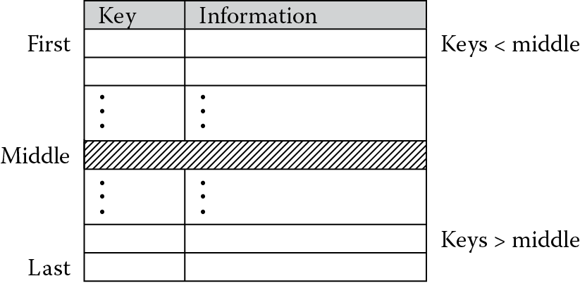
If you have a list of entries in a table, as shown in Figure 12.2, where each entry consists of a numerical key and some type of data to go along with that key, e.g., character data such as an address or numerical data such as a phone number, you could try to find a key by sequentially comparing each key in the table to your value. Obviously this would take the longest amount of time, especially if the key of interest happened to be at the end of the table. If the keys are sorted already, say in increasing order, then you can significantly reduce your search efforts by starting at the middle of the table. This can immediately halve your search effort. Again referring to Figure 12.2, you can see that if our key is less than the middle key, we don’t even have to look in the latter half of the table. We know it’s somewhere between the first and middle keys, if it’s there at all. Next, we further refine the search by making the last key in our search the key just before the middle one. The new middle key is defined as the average of the first and last keys, and the procedure is repeated until the key is either found or we confirm that it’s not in the table. If the middle key happens to match our key, then the algorithm is finished. In a like manner, if the key we’re looking for is between the middle and last keys in the table, we move the start of our search to the entry just after the middle key and compute a new middle key for comparisons. The C equivalent of this technique could be described as

first = 0;

last = num_entries − 1;

index = 0;

while  ((index = = 0) & (first <= last)){

	middle = (first + last)/2;

	if (key = = table[middle]) index = middle;

	else if (key < table[middle]) last = middle – 1;

	else first = middle + 1;

	}

where num_entries is the number of entries in the table.

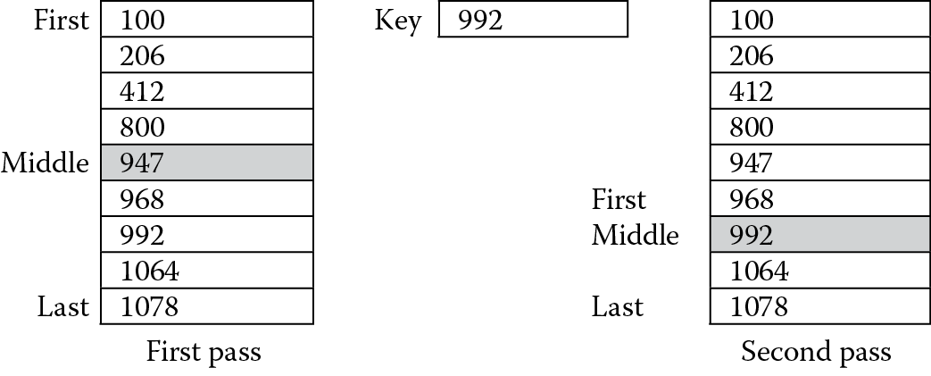
Figure 12.3 shows an example of how this works. Suppose we have a table with nine entries in it, and the key of interest is 992. On the first pass of the search, we compute the middle of the table to be index number 4, since this is the average of the first and last entry numbers, 0 and 8, respectively. A comparison is then made against the table entry with this index. Since our number is greater than the middle number, the search focuses on the half of the table where the keys are even larger. The new starting position is entry number 5, while the last entry remains the same. A new middle index is found by averaging 5 and 8, which is 6 (remember they have to be integers). The comparison against the table entry with this index happens to match, so we’ve actually found the entry and the algorithm terminates.

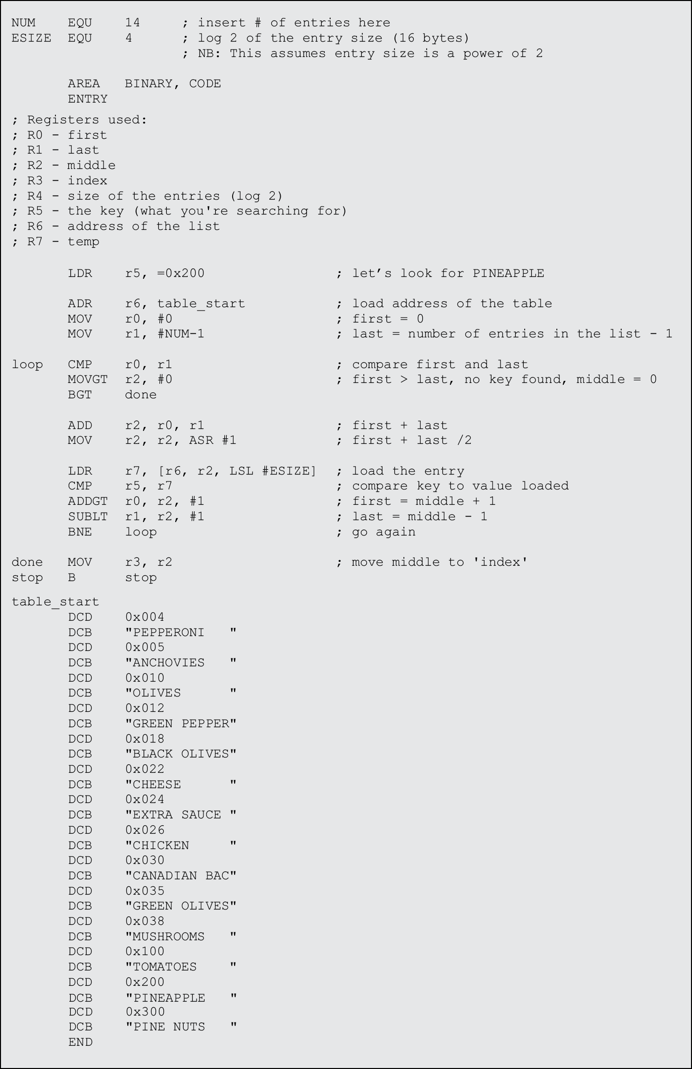
In coding the binary search, we should examine a few aspects of the algorithm and of the data first, since most of the work can be done with just a few instructions. The rest of them are used to control the loop. Consider a table starting at address 0x4000, where each entry is 16 bytes, and say that 4 bytes, or a word, is used as a key. This leaves the remaining 12 bytes for character data, as shown in Figure 12.4. Examining the address of the tag, we can see that if the index i ranges from 0 to some number n–1, and the starting address of the table is table_addr, the address of the ith entry would be

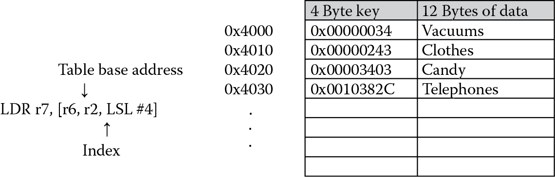
address = table_addr + i * size_of_entry.

For our table, the second entry would start at address 0x4000 + 2 × 16 = 0x4020.

Using this approach, we can simply use an LDR instruction with pre-indexed addressing, offsetting the table’s base address with the scaled index, which is held in a register. The scaling (which is based on the entry size in bytes) can actually be specified with a constant—ESIZE—so that if we change this later, we don’t have to recode the instructions. With this approach comes a word of caution, since we assume that the entry size is a power of two. If this is not the case, all hope is not lost. You can implement a two-level table, where an entry now consists of a key and an address pointing to data in memory, and the data can be any size you like. The size of each entry is again fixed, and it can be set to a power of two. However, for our example, the entry size is a power of two.

We can load our table entries with a single pre-indexed instruction:

LDR r7, [r6, r2, LSL #ESIZE]

This just made short work of coding the remaining algorithm. The first four instructions in Figure 12.5 are just initialization—the base address of the table is loaded into a register, the first index is set to 0, and the last index is set to the last entry, in this case, the number of entries we have, called NUM, minus one. The instructions inside of the loop test to see whether the first index is still smaller than or equal to the last index. If it is, a new middle index is generated and used to load the table entry into a register. The data is loaded from the table and tested against our key. We can effectively use conditional execution to change the first and last indices, since the comparison will test for mutually exclusive conditions. The loop terminates with either a zero or the key index loaded into register r3. The data that is used in the example might be someone’s address on a street, followed by his or her favorite pizza toppings. Note that each key is 4 bytes and the character data is 12 bytes for each entry.

Execution times for search algorithms are important. Consider that a linear search through a table would take twice as long to execute if the table doubled in size, where a binary search would only require one more pass through its loop. The execution time increases logarithmically.

12.5 Exercises

1. Using the sine table as a guide, construct a cosine table that produces the value for cos(x), where 0 < x < 360. Test your code for values of 84 degrees and 105 degrees.
2. It was mentioned in Section 12.4 that a binary search only works if the entries in a list are sorted first. A bubble sort is a simple way to sort entries. The basic idea is to compare two adjacent entries in a list—call them entry[j] and entry[j + 1]. If entry[j] is larger, then swap the entries. If this is repeated until the last two entries are compared, the largest element in the list will now be last. The smallest entry will ultimately get swapped, or “bubbled,” to the top. This algorithm could be described in C as

	last = num;

	while (last > 0){

	pairs = last – 1;

	for (j = 0; j <= pairs; j + +) {

		if(entry[j] > entry[j + 1]) {

				temp = entry[j];

				entry[j] = entry[j + 1];

				entry[j + 1] = temp;

				last = j;

		}

	}

	}

1. where num is the number of entries in the list. Write an assembly language program to implement a bubble sort algorithm, and test it using a list of 20 elements. Each element should be a word in length.

1. Using the bubble sort algorithm written in Exercise 2, write an assembly program that sorts entries in a list and then uses a binary search to find a particular key. Remember that your sorting routine must sort both the key and the data associated with each entry. Create a list with 30 entries or so, and data for each key should be at least 12 bytes of information.
2. Create a queue of 32-bit data values in memory. Write a function to remove the first item in the queue.
3. Using the sine table as a guide, construct a tangent table that produces the value for tan(x), where 0 ≤ x ≤ 45. Test your code for values of 12 degrees and 43 degrees. You may return a value of 0x7FFFFFFF for the case where the angle is equal to 45 degrees, since 1 cannot be represented in Q31 notation.
4. Implement a sine table that holds values ranging from 0 to 180 degrees. The implementation contains fewer instructions than the routine in Section 12.2, but to generate the value, it uses more memory to hold the sine values themselves. Compare the total code size for both cases.
5. Implement a cosine table that holds values ranging from 0 to 180 degrees. The implementation contains fewer instructions than the routine in Section 12.2, but to generate the value, it uses more memory to hold the cosine values themselves. Compare the total code size for both cases.
6. Rewrite the binary search routine for the Cortex-M4.

---