Table of Contents for
ARM Assembly Language, 2nd Edition
 ARM Assembly Language, 2nd Edition
Published by
Chapman and Hall/CRC, 2016
ARM Assembly Language, 2nd Edition
Published by
Chapman and Hall/CRC, 2016
- Contents
- ARM Assembly Language: Fundamentals and Techniques, Second Edition
- Preliminaries
- To our families
- Preface
- Acknowledgments
- Authors
- Chapter 1 - An Overview of Computing Systems
- Chapter 2 - The Programmer’s Model
- Chapter 3 - Introduction to Instruction Sets: v4T and v7-M
- Chapter 4 - Assembler Rules and Directives
- Chapter 5 - Loads, Stores, and Addressing
- Chapter 6 - Constants and Literal Pools
- Chapter 7 - Integer Logic and Arithmetic
- Chapter 8 - Branches and Loops
- Chapter 9 - Introduction to Floating-Point: Basics, Data Types, and Data Transfer
- Chapter 10 - Introduction to Floating-Point: Rounding and Exceptions
- Chapter 11 - Floating-Point Data-Processing Instructions
- Chapter 12 - Tables
- Chapter 13 - Subroutines and Stacks
- Chapter 14 - Exception Handling: ARM7TDMI
- Chapter 15 - Exception Handling: v7-M
- Chapter 16 - Memory-Mapped Peripherals
- Chapter 17 - ARM, Thumb and Thumb-2 Instructions
- Chapter 18 - Mixing C and Assembly
- Appendix A: Running Code Composer Studio
- Appendix B: Running Keil Tools
- Appendix C: ASCII Character Codes
- Appendix D
- Glossary
- References
Chapter 9
Introduction to Floating-Point
Basics, Data Types, and Data Transfer
9.1 Introduction
In Chapter 1 we looked briefly at the formats of the floating-point data types called single-precision and double-precision. These data types are referred to as float and double, respectively, in C, C++, and Java. These formats have been the standard since the acceptance of the IEEE Standard for Binary Floating-Point Arithmetic (IEEE Standard 1985), known as the IEEE 754-1985 standard, though floating-point was in use long before an effort to produce a standard was considered. Each computer maker had their own data types, rounding modes, exception handling, and odd numeric quirks. In this chapter we take a closer look at the single-precision floating-point data type, the native data type of the Cortex-M4 floating-point unit, and a new format called half-precision. An aim of this chapter is to answer why a programmer would choose to use floating-point over integer in arithmetic computations, and what special considerations are necessary to properly use these data types. This introductory look, here and in Chapters 10 and 11, will let us add floating-point to our programming and make use of a powerful feature of the Cortex-M4.
9.2 A Brief History of Floating-Point in Computing
Hardware floating-point is a relatively new part of embedded microprocessors. One of the earliest embedded processors offered with optional floating-point was the ARM10, introduced in 1999. In the last fifteen years embedded processors, such as the ARM11 and Cortex-M4, have been available with hardware floating-point. The adoption of floating-point in the embedded space follows a long tradition of computing features which were first introduced in supercomputer and mainframe computers, and over time migrated to minicomputers, later to desktop processors, and ultimately to the processors which power your smart phone and tablet.
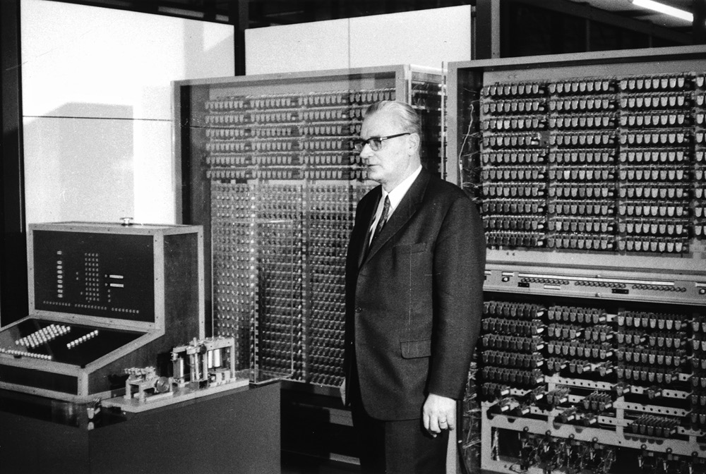
The earliest processor with floating-point capability was the Z3, built by Konrad Zuse in Berlin in the years 1938–1941.* Figure 9.1 shows Dr. Zuse and a reconstruction of the Z3 computer. It featured a 22-bit floating-point unit, with 1 sign bit, 7 bits of exponent, and 14 bits of significand. Many of the early machines eschewed floating-point in favor of fixed-point, including the IAS Machine, built by John von Neumann in Princeton, New Jersey. Of the successful commercial computers, the UNIVAC 1100 series and 2200 series included two floating-point formats, a single-precision format using 36 bits and a double-precision format using 72 bits. Numerous machines soon followed with varying data formats. The IBM 7094, shown in Figure 9.2, like the UNIVAC, used 36-bit words, but the IBM 360, which followed in 1964, used 32-bit words, one for single-precision and two for double-precision. The interesting oddity of IBM floating-point was the use of a hexadecimal exponent, that is, the exponent used base 16 rather than base 2, with each increment of the exponent representing 24.† In the supercomputer space, machines by Control Data Corporation (CDC) and later by Cray would use a 60-bit floating-point format and be known for their speed of floating-point computation. That race has not stopped. While Cray held the record for years with a speed of 160 million floating-point operations per second (megaflops), modern supercomputers boast speeds in the petaflop (1015 flops) range! Figure 9.3 is a photograph of Seymore Cray and the original Cray-1 computer.


However, even with the wide adoption of floating-point there were problems. Companies supported their own formats of floating-point data types, had different models for exceptions, and rounded the results in different ways. While you may not be familiar with floating-point exceptions or rounding just yet, when these concepts are addressed you will see the benefits of a standard that defines the data types, exception handling, and rounding modes. For an example of the problems that arose due to the varied landscape of behaviors, consider the Cray machines. These processors were blazingly fast in their floating-point computations, but they suffered in computational accuracy due to some shortcuts in their rounding logic. They were fast, but not always accurate! In the early 1980s, an IEEE standards committee convened to produce a standard for floating-point which would introduce a consistency to computations done in floating-point, enable work to be performed across a wide variety of computers, and result in a system which could be used by non-numerical experts to produce reliable numerical code. A key leader in this effort was Dr. William Kahan, shown in Figure 9.4, of the University of California at Berkeley, at the time consulting with Intel Corporation on the development of the i8087 floating-point coprocessor. The specification defined the format of the data types, including special values such as infinities and not-a-numbers (NaNs, to be considered in a later section); how rounding was to be done; what conditions would result in exceptions; and how exceptions would be handled and reported. In 2008, a revision of the standard, referred to as IEEE 754-2008, was released, adding decimal data types and addressing a number of issues unforeseen 25 years ago. Most processors with floating-point hardware, from supercomputers to microcontrollers, implement some subset of the IEEE 754 standard.

9.3 The Contribution of Floating-Point to the Embedded Processor
The cost of an integrated circuit is directly related to the size of the die. The larger the size of the die, the fewer of them that can be put on a wafer. With constant wafer costs, the more die on the wafer, the lower the cost of each die. So it is a reasonable question to ask why manufacturers spend the die area on an FPU, or, more specifically, what value does the floating-point unit of the Cortex-M4 bring? To answer these questions it is necessary to first consider how floating-point computations differ from integer computations. As we saw in Chapter 2, the integer data types are commonly in three formats:
- Byte, or 8 bits
- Halfword, or 16 bits
- Word, or 32 bits
Each of these formats may be treated as signed or unsigned. For the moment we will consider only 32-bit words, but each data type shares these characteristics. The range of an unsigned word value is 0 to 4,294,967,295 (232–1). Signed word values are in the range −2,147,483,648 to 2,147,483,647, or −231 to 231−1. While these are large numbers, many fields of study cannot live within these bounds. For example, the national debt is $17,320,676,548,008.59 (as of January 4, 2014), a value over 2000 times larger than can be represented in a 32-bit unsigned word. In the field of astronomy, common distances are measured in parsecs, with one parsec equal to 3.26 light years, or about 30,856,780,000,000 km. While such a number cannot be represented in a 32-bit unsigned word, it is often unnecessary to be as precise as financial computations. Less precise values will often suffice. So, while the charge on an electron, denoted e, is 1.602176565 × 10⁻¹⁹ coulombs, in many instances computations on e can tolerate reduced precision, perhaps only a few digits. So 1.60 × 10⁻¹⁹ may be precise enough for some calculations. Floating-point enables us to trade off precision for range, so we can represent values larger than 32-bit integers and also much smaller than 1, but frequently with less than full precision.
Could this mean floating-point is always the best format to use? Simply put, no. Consider the 32-bit integer and 32-bit single-precision floating-point formats. Both have the same storage requirements (32 bits, or one word), both have the same number of unique bit patterns (232), but integers have a fixed numeric separation, that is, each integer is exactly the same distance from the integer just smaller and the integer just larger. That numeric separation is exactly and always 1. Consider that we represent the decimal value 1037 in 32-bit binary as
0000 0000 0000 0000 0000 0100 0000 1101;
the integer value just smaller is 1036, represented in 32-bit binary as
0000 0000 0000 0000 0000 0100 0000 1100;
and the integer value just larger is 1038, and it is represented in 32-bit binary as
0000 0000 0000 0000 0000 0100 0000 1110.
In each case the difference between sequential values is exactly 1 (verify you believe this from the last 4 bits). This is why integers make a great choice for counters and address values, but not always for arithmetic calculations. Why would a 32-bit floating-point value be better for arithmetic? As we showed above, the range of a 32-bit integer is insufficient for many problems—it is simply not big enough on the end of the number curve, and not small enough to represent values between 0 and 1. If we use 64-bit integers we extend the range significantly, but again not enough for all problems. We will see that floating-point values have a much greater range than even 64-bit integers. They accomplish this by not having a fixed numeric separation, but a variable one that depends on the value of the exponent. We’ll explain this in Section 9.5.
So, back to our question—Why include floating-point capability in the processor? To begin our evaluation, let’s ask some questions. First, does the application have inputs, outputs, or intermediate values larger than representable by the available integers? Second, does the application have inputs, outputs, or intermediate values between 0 and 1? If either of these questions is yes, can we use fixed-point representations to satisfy the range required? Third, do any of the algorithms in the application require correct rounding, rather than truncation? Fourth, how easy is it to ensure that no intermediate value is outside the range of the available integers? In many cases the analysis required to ensure that all inputs, outputs, and intermediate values remain in the range available is not trivial, but can be quite difficult. The answers to these questions will point the system designer to one of two conclusions–that the integer formats are sufficient, or the problems are better processed with floating-point. The following chapters introduce the key elements of floating-point, where floating-point differs from integer and fixed-point computation, and what benefits come naturally to computations in floating-point. Knowing this will make the decision easier for the system designer.
9.4 Floating-Point Data Types
The IEEE 754-2008 specification defines four binary floating-point formats: 16-bit, 32-bit, 64-bit, and 128-bit, commonly referred to as half-precision, single-precision, double-precision, and quad-precision, respectively. C, C++, and Java refer to the 32-bit format as float and the 64-bit format as double. The Cortex-M4 does not support the two larger formats, but does support a half-precision floating-point format for data storage and the single-precision data type for computation. Figure 9.5 shows the half-precision, single-precision, and double-precision data formats.
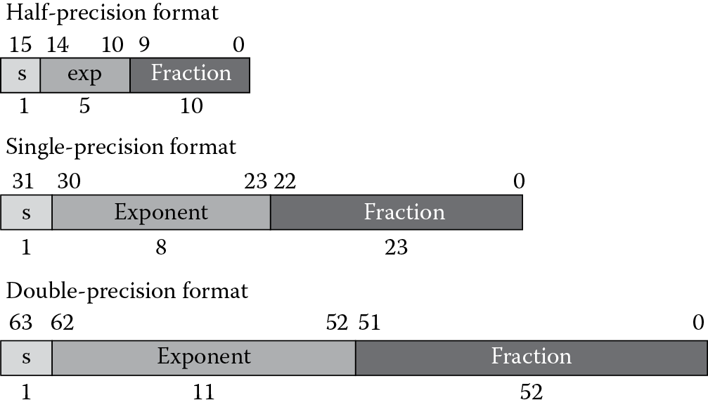
From Figure 9.5 you can see the floating-point formats are composed of three component parts: the sign bit, represented by s; the exponent, typically in a biased form (see the explanation of bias below); and the fraction. The value of a floating-point data value is computed according to the formula for normal values, covered in Section 9.6.1. We will consider special values in a later sections. This format is called sign magnitude representation, since the sign bit is separate from the bits that comprise the magnitude of the value. The equation for normal values in a floating-point format is given by‡
F = (−1)s × 2(exp–bias) × 1.f (9.1)
where:
- s is the sign,
- 0 for positive
- 1 for negative
- exp is the exponent,
- The bias is a constant specified in the format
- The purpose is to create a positive exponent
- f is the fraction, or sometimes referred to as the mantissa
We refer to the value 1.f as the significand, and this part of the equation is always in the range [1.0, 2.0) (where the value may include 1.0 but not 2.0). The set of possible values is referred to as the representable values, and each computation must result in either one of these representable values or a special value. The bias is a constant added to the true exponent to form an exponent that is always positive. For the single-precision format, the bias is 127, resulting in an exponent range of 1 to 254 for normal numbers. The exponent values 0 and 255 are used for special formats, as will be considered later. Table 9.1 shows the characteristics of the three standard data types.
Floating-Point Formats and Their Characteristics
|
Format |
|||
|
Half-Precisiona |
Single-Precision |
Double-Precision |
|
|
Format width in bits |
16 |
32 |
64 |
|
Exponent width in bits |
5 |
8 |
11 |
|
Fraction bits |
10 |
23 |
52 |
|
Exp maximum |
+15 |
+127 |
+1023 |
|
Exp minimum |
−14 |
−126 |
−1022 |
|
Exponent bias |
15 |
127 |
1023 |
a The Cortex-M4 has an alternative format for half-precision values. This format may be selected by setting the AHF bit in the FPSCR, and the format will be interpreted as having an exponent range that includes the max exponent, 21 6. This precision does not support NaNs or infinities. The maximum value is (2-2−1 0) × 21 6 or 131008.
Example 9.1
Form the single-precision representation of 6.5.
Solution
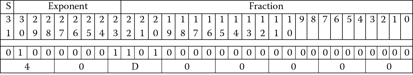
The sign is positive, so the sign bit will be 0. The power of 2 that will result in a significand between 1 and almost 2 is 4.0 (22), resulting in a significand of 1.625. Expressed in floating-point representation, the value 6.5 is
6.5 = −10 × 22 × 1.625
To finish the example, convert the resulting factor to a significand in binary.
1.625 = 1 + ½ + ⅛, or in binary, 1.101.
The exponent is 2, and when the bias is added to form the exponent part of the single-precision representation, the biased exponent becomes 129, or 0x81.
The resulting single-precision value is 0x40D00000, shown in binary and hexadecimal in Figure 9.6.
Example 9.2
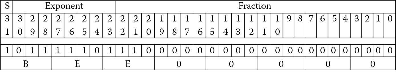
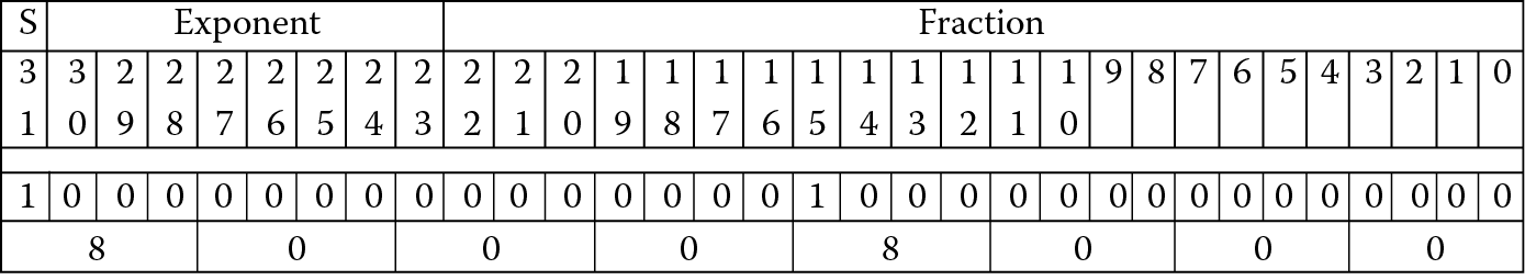
Form the single-precision representation of −0.4375.
Solution
The sign is negative, so the sign bit will be 1. The power of 2 that will result in a significand between 1 and almost 2 is 2−2 (0.25), giving a significand of 1.75.
−0.4375 = −11 × 2−2 × 1.75
1.75 = 1 + ½ + ¼, or in binary, 1.11.
The exponent is −2, and when the bias is added to form the exponent of the single-precision representation, the biased exponent becomes 125, or 0x7D. The resulting single-precision value is 0xBEE00000. See Figure 9.7.
It’s unlikely you will ever have to do these conversions by hand. The assembler will perform the conversion for you. Also, a number of useful websites will do the conversions for you. See, e.g., (http://babbage.cs.qc.cuny.edu/IEEE-754.old/Decimal.html) for conversions from decimal to floating-point. See also (http://babbage.cs.qc.cuny.edu/IEEE-754.old/32bit.html) for an excellent website that has a very useful calculator to perform the conversion from single-precision floating-point to decimal. Also, the website at (http://www.h-schmidt.net/FloatConverter) allows you to set each bit separately in a single-precision representation and see immediately the contribution to the final value.
9.5 The Space of Floating-Point Representable Values
In school we learned about the number line and the whole numbers. On this number line, each whole number was separated from its neighbor whole number by the value 1. Regardless of where you were on the number line, any whole number was 1 greater than the whole number to the left and 1 less than the whole number to the right. Such is not the case for the floating-point number line. Recall from Equation 9.1 above that the significand is multiplied by a power of 2. The larger the exponent, the greater the multiplication factor applied to the significand. Two significands that are contiguous, i.e., the larger significand is the next higher value, would differ by a factor of the exponent rather than a fixed value. Let’s represent this idea using a simple format with 2 bits of fraction and an exponent range of −3 ≤ E ≤ 0. The floating-point number line looks like Figure 9.8.
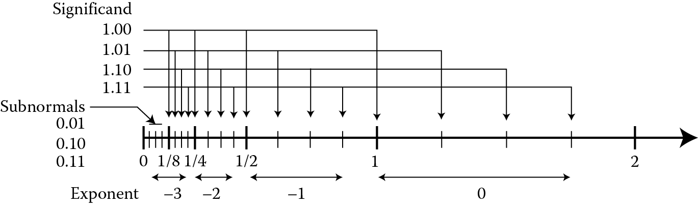
Floating-point number line for positive values, 2 exponent bits and 2 fractional bits (see Ercegovac and Lang 2004).
There are several things to notice in the number line in Figure 9.8. First, the number of representable values associated with each exponent is fixed at 2n, where n is the number of bits in the fraction. In this example, two bits give four representable values for each exponent. Notice that four values exist with an exponent of −1 using our format: ½, ⅝, ¾, and ⅞. Second, notice the numeric separation between each representable value is a function of the exponent value, and as the exponent increases by one, the numeric separation doubles. The only exception is in the subnormal range, and we will discuss subnormals in Section 9.6.2. If we consider a single-precision data value with the exponent equal to 0 (a biased exponent of 127), the range of values with this exponent are:
1.0 … 1.99999998808 (21 – 2−23)
That is, the minimum value representable is 1.0, while the maximum value is just less than 2.0. With a fraction of 23 bits, the numeric separation between representable values is 2−23, or ~1.192 × 10⁻⁷, a fairly small amount.
Contrast this to an exponent of 23 (a biased exponent of 150). Now each value will be in the range
8388608 … 16777215
In this instance, the numeric separation between representable values is 1.0, much larger than the 1.192 × 10⁻⁷ of the previous example.
If we continue this thought with an exponent closer to the maximum, say 73 (a biased exponent of 200), we have this range of values:
9.445 × 10²¹ … 1.889 × 10²²
Here the numeric separation between representable values is roughly 1.126 × 10¹⁵! If we go in the other direction, say with an exponent value of −75 (a biased exponent of 52), the range becomes
2.647 × 10⁻²³ … 5.294 × 10⁻²³
with a numeric separation of 3.155 × 10⁻³⁰! Table 9.2 is a summary of the findings.
Examples of the Range of Numeric Separation in Single-Precision Values
|
Exponent |
exp-bias |
Range |
Numeric Separation |
|
52 |
−75 |
2.647 × 10− 23 … 5.294 × 10− 23 |
3.155 × 10− 30 |
|
127 |
0 |
1.0 … 1.9999998 |
1.192 × 10− 7 |
|
150 |
23 |
8388608 … 16777215 |
1.0 |
|
200 |
73 |
9.445 × 10²¹ … 1.889 × 10²² |
1.126 × 10¹⁵ |
From Table 9.2 it is evident that the range of single-precision values and the numeric separation vary a great deal. Notice that the numeric separation between values for an exponent of 73 is greater than the total range for values with an exponent of 23. The key to understanding floating-point as a programmer is that floating-point precision is not fixed but a function of the exponent. That is, while the numeric separation in an integer data type is always 1, the numeric separation of a floating-point data type varies with the exponent. This is rarely a problem for scientific computations—we typically are interested in only a few digits regardless of the magnitude of the results. So if we specify the precision of our results is to be 4 digits, 1 to the left of the decimal point and three to the right, we may compute
5.429 × 10¹⁵
but another calculation may result in
−2.907 × 10⁻⁸
and we would not consider this in error even though the value of the second calculation is much smaller than the smallest variation we are interested in of the first result (a factor of 1012). Rather, the precision of each of the calculations is the same—4 digits. Thinking of floating-point as a base-2 version of scientific notation will help in grasping the useful properties of floating-point, and in using them properly.
9.6 Floating-Point Representable Values
All representable values have a single encoding in each floating-point format, but not all floating-point encodings represent a number. This is another difference between floating-point and integer representation. The IEEE 754-2008 specification defines five classes of floating-point encodings: normal numbers, subnormal numbers, zeros, NaNs, and infinities. Each class has some shared properties and some unique properties. Let’s consider each one separately.
9.6.1 Normal Values
We use the term normal value to define a floating-point value that satisfies the equation
F = (−1)s × 2(exp–bias) × 1.f (9.1)
which we saw earlier in Section 9.4. In the space of normal values, each floating-point number has a single encoding, that is, an encoding represents only one floating-point value and each representable value has only one encoding. Put another way, no aliasing exists within the single-precision floating-point data type. It is possible to have multiple encodings represent a single value when represented in decimal floating-point formats, but this is beyond the scope of this text. See the IEEE 754-2008 specification for more on this format.
Recall that a 32-bit signed integer has a range of −2,147,483,648 to 2,147,483,647 (+/−2.147 × 109). Figure 9.9 shows the range of signed 32-bit integers, half-precision (16-bit) and single-precision (32-bit) floating-point data types for the normal range. Notice the range of the signed 32-bit integer and the half-precision data types is roughly the same; however, notice the much greater range available in the single-precision floating-point data type.
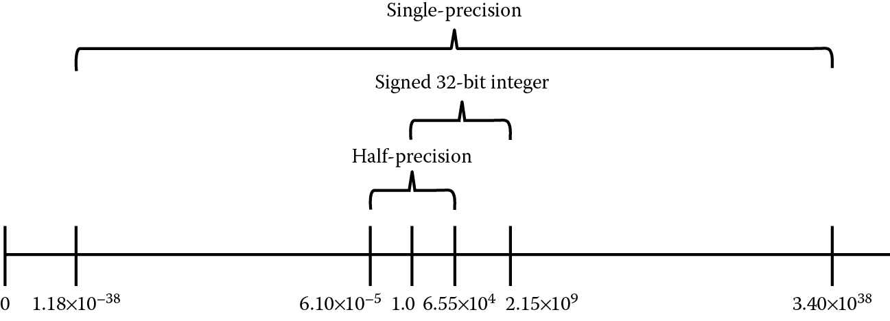
Relative normal range for signed 32-bit integer, half-precision floating-point, and single-precision floating-point data types.
Remember, the tradeoff between the integer data types and the floating-point data types is in the precision of the result. In short, as we showed in Figure 9.8, the precision of a floating-point data value is a function of the exponent. As the exponent increases, the precision decreases, resulting in an increased numeric separation between representable values.
Table 9.3 shows some examples of normal data values for half-precision and single-precision formats. Note that each of these values may be made negative by setting the most-significant bit. For example, −1.0 is 0xBF800000. Using the technique shown in Section 9.4, try out some of these. You can check your work using the conversion tools listed in the References.
Several Normal Half-Precision and Single-Precision Floating-Point Values
|
Format |
||
|
Half-Precision |
Single-Precision |
|
|
1.0 |
0x3C00 |
0x3F800000 |
|
2.0 |
0x4000 |
0x40000000 |
|
0.5 |
0x3800 |
0x3F000000 |
|
1024 |
0x6400 |
0x44800000 |
|
0.005 |
0x1D1F |
0x3BA3D70A |
|
6.10 × 10− 5 |
0x0400 |
0x38800000 |
|
6.55 × 10⁴ |
0x7BFF |
0x477FE000 |
|
1.175 × 10− 38 |
Out of range |
0x00800000 |
|
3.40 × 1038 |
Out of range |
0x7F7FFFFF |
9.6.2 Subnormal Values
The inclusion of subnormal values§ was an issue of great controversy in the original IEEE 754-1985 deliberations. When a value is non-zero and too small to be represented in the normal range, it value may be represented by a subnormal encoding. These values satisfy Equation 9.2:
F = (−1)s × 2−126 × 0.f (9.2)
Notice first the exponent value is fixed at −126, one greater than the negative bias value. This value is referred to as emin, and is the exponent value of the smallest normal representation. Also notice that the 1.0 factor is missing, changing the significand range to [0.0, 1.0). The subnormal range extends the lower bounds of the representable numbers by further dividing the range between zero and the smallest normal representable value into 223 additional representable values. If we look again at Figure 9.8, we see in the region marked Subnormals that the range between 0 and the minimum normal value is represented by n values, as in each exponent range of the normal values. The numeric separation in the subnormal range is equal to that of the normal values with minimum normal exponent. The minimum value in the normal range for the single-precision floating-point format is 1.18 × 10−38. The subnormal values increase the minimum range to 1.4 × 10−45. Be aware, however, when an operand in the subnormal range decreases toward the minimum value, the number of significant digits decreases. In other words, the precision of subnormal values may be significantly less than the precision of normal values, or even larger subnormal values. The range of subnormal values for the half-precision and single-precision data types is shown in Table 9.4. Table 9.5 shows some examples of subnormal data values. As with the normal values, each of these values may be made negative by setting the most significant bit.
Subnormal Range for Half-Precision and Single-Precision
|
Format |
||
|
Half-Precision |
Single-Precision |
|
|
Minimum |
+/−5.96 × 10− 8 |
+/−1.45 × 10− 45 |
|
Maximum |
+/−6.10 × 10− 5 |
+/−1.175 × 10− 38 |
Examples of Subnormal Values for Half-Precision and Single-Precision
|
Format |
||
|
Half-Precision |
Single-Precision |
|
|
6.10 × 10− 5 |
0x03FF |
|
|
1.43 × 10− 6 |
0x0018 |
|
|
5.96 × 10− 8 |
0x0001 |
|
|
1.175 × 10− 38 |
0x007FFFFF |
|
|
4.59 × 10− 41 |
0x00008000 |
|
|
1.45 × 10− 45 |
0x00000001 |
|
Example 9.3
Convert the value −4.59 × 10−41 to single-precision.
Solution
The value is below the minimum threshold representable as a normal value in the single-precision format, but is greater than the minimum representable subnormal value and is in the subnormal range for the single-precision format.
Recalling our conversion steps above, we can use the same methodology for subnormal values so long as we recall that the exponent is fixed at the value 2−126 and no implicit 1 is present.
First, divide −4.592 × 10−41 by 2−126 and we have −0.00390625, which is equal to 2−8. This leaves us with
−4.592 × 10−41 = −11 × 2−126 × 0.00390625
The result single-precision value is 0x80008000, shown in binary and hexadecimal in Figure 9.10.
The conversion to and from half-precision is done in an identical manner, but remember the subnormal exponent for the half-precision format is −14 and the format is only 16 bits.
A computation that results in a subnormal value may set the Underflow flag and may signal an exception. We will address exceptions in a later chapter.
9.6.3 Zeros
It’s odd to think of zero as anything other than, well, zero. In floating-point zeros are signed. You may compute a function and see a negative zero as a result! Zeros are formed by a zero exponent and zero fraction. A critical bit of information here—if the fraction is not zero, the value is a subnormal, as we saw above. While numerous subnormal encodings are possible, only two zero encodings, a positive zero with a sign bit of zero, and a negative zero with a sign bit of one, are possible. How is it possible to have a negative zero? There are several ways outlined in the IEEE 754-2008 specification. One way is to be in Round to Minus Infinity mode (we will consider rounding in Chapter 10) and sum two equal values that have opposite signs.
Example 9.4
Add the two single-precision values 0x3F80000C and 0xBF80000C with different rounding modes.
Solution
Let register s0 contain 0x3F80000C and register s1 contain 0xBF80000C. The two operands have the same magnitude but opposite sign, so the result of adding the two operands using the Cortex-M4 VADD instruction (we will consider this instruction in Chapter 11)
VADD s2, s0, s1
in each case is zero. But notice that the sign of the zero is determined by the rounding mode. We will consider rounding modes in detail in Chapter 10, but for now consider the four in Table 9.6. (The names give a clue to the rounding that is done. For example, roundTowardPositive always rounds up if the result is not exact. The rounding mode roundTiesToEven uses the method we learned in school—round to the nearest valid number, and if the result is exactly halfway between two valid numbers, pick the one that is even.)
Operations with Zero Result in Each Rounding Mode
|
Rounding Mode |
Result |
|
|
roundTiesToEven |
0x00000000 |
Positive Zero |
|
roundTowardPositive |
0x00000000 |
Positive Zero |
|
roundTowardNegative |
0x80000000 |
Negative Zero |
|
roundTowardZero |
0x00000000 |
Positive Zero |
Likewise, a multiplication of two values, one positive and the other negative, with a product too small to represent as a subnormal, will return a negative zero. And finally, the square root of −0 returns −0. Why bother with signed zeros? First, the negative zero is an artifact of the sign-magnitude format, but more importantly, the sign of zero is an indicator of the direction of the operation or the sign of the value before it was rounded to zero. This affords the numeric analyst with information on the computation, which is not obvious from an unsigned zero result, and this may be useful even if the result of the computation is zero.
The format of the two zeros for half-precision and single-precision are shown in Table 9.7.
Format of Signed Zero in Half-Precision and Single-Precision
|
Format |
||
|
Half-Precision |
Single-Precision |
|
|
+0.0 |
0x0000 |
0x00000000 |
|
−0.0 |
0x8000 |
0x80000000 |
9.6.4 Infinities
Another distinction between floating-point and integer values is the presence of an infinity encoding in the floating-point formats. A floating-point infinity is encoded with an exponent of all ones and a fraction of all zeros. The sign indicates whether it is a positive or negative infinity. While it is tempting to consider the positive infinity as the value just greater than the maximum normal value, it is best considered as a mathematical symbol and not as a number. In this way computations involving infinity will behave as would be expected. In other words, any operation computed with an infinity value by a normal or subnormal value will return the infinity value. However, some operations are invalid, that is, there is no generally accepted result value for the operation. An example is multiplication of infinity by zero. We note that the IEEE 754-2008 specification defines the nature of the infinity in an affine sense, that is,
−∞ < all finite numbers < +∞
Recall from Section 7.2.2 that overflow in an integer computation produces an incorrect value and sets a hardware flag. To determine whether overflow occurred, a check on the flags in the status register must be made before you can take appropriate action. Multiplying two very large values that result in a value greater than the maximum for the floating-point format will return an infinity,¶ and further calculations on the infinity will indicate the overflow. While there is an overflow flag (more on this in Chapter 10), in most cases the result of a computation that overflows will indicate as much without requiring the programmer to check any flags. The result will make sense as if you had done it on paper. The format of the half-precision and single-precision infinities is shown in Table 9.8.
Format of Signed Infinity in Half-Precision and Single-Precision
|
Format |
||
|
Half-Precision |
Single-Precision |
|
|
−Infinity |
0xFC00 |
0xFF800000 |
|
+Infinity |
0x7C00 |
0x7F800000 |
9.6.5 Not-a-Numbers (NaNs)
Perhaps the oddest of the various floating-point classes is the not-a-number, or NaN. Why would a numerical computation method include a data representation that is “not a number?” A reasonable question, certainly. They have several uses, and we will consider two of them. In the first use, a programmer may choose to return a NaN with a unique payload (the bits in the fraction portion of the format) as an indicator that a specific, typically unexpected, condition existed in a routine within the program. For instance, the programmer believes the range of data for a variable at a point in the program should not be greater than 100. But if it is, he can use a NaN to replace the value and encode the payload to locate the line or algorithm in the routine that caused the behavior. Secondly, NaNs have historically found use as the default value put in registers or in data structures. Should the register or data structure be read before it is written with valid data, a NaN would be returned. If the NaN is of a type called signaling NaNs, the Invalid Operation exception would be signaled, giving the programmer another tool for debugging. This use would alert the programmer to the fact that uninitialized data was used in a computation, likely an error. The Motorola MC68881 and later 68K floating-point processors initialized the floating-point register file with signaling NaNs upon reset for this purpose. Both signaling NaNs, and a second type known as quiet NaNs, have been used to represent non-numeric data, such as symbols in a symbolic math system. These programs operate on both numbers and symbols, but the routines operating on numbers can’t handle the symbols. NaNs have been used to represent the symbols in the program, and when a symbol is encountered it would cause the program to jump to a routine written specifically to perform the needed computation on symbols rather than numbers. This way it would be easy to intermix symbols and numbers, with the arithmetic of the processor operating on the numbers and the symbol routines operating whenever an operand is a symbol.
How does one use NaNs? One humorous programmer described NaNs this way: when you think of computing with NaNs, replace the NaN with a “Buick” in a calculation.** So, what is a NaN divided by 5? Well, you could ask instead, “What is a Buick divided by 5?” You quickly see that it’s not possible to reasonably answer this question, since a Buick divided by 5 is not-a-number, so we will simply return the Buick (unscratched, if we know what’s good for us). Simply put, in an operation involving a NaN, the NaN, or one of the NaNs if both operands are NaN, is returned. This is the behavior of an IEEE 754-2008-compliant system in most cases when a NaN is involved in a computation. The specification does not direct which of the NaNs is returned when two or more operands are NaN, leaving it to the floating-point designer to select which is returned.
A NaN is encoded with an exponent of all ones and a non-zero fraction. Note that an exponent of all ones with a zero fraction is an infinity encoding, so to avoid confusing the two representations, a NaN must not have a zero fraction. As we mentioned above, NaNs come in two flavors: signaling NaNs (sNaN) and non-signaling, or quiet, NaNs (qNaN). The difference is the value of the first, or most significant, of the fraction bits. If the bit is a one, the NaN is quiet. Likewise, if the bit is a zero, the NaN is signaling, but only if at least one other fraction bit is a one. In the half-precision format, bit 9 is the bit that identifies the NaN type; in the single-precision format it’s bit 22. The format of the NaN encodings for the half-precision format and the single-precision format is shown in Table 9.9.
Format of NaN Encodings in Half-Precision and Single-Precision
|
Format |
||
|
Half-Precision |
Single-Precision |
|
|
Sign bit |
0/1 |
0/1 |
|
Exponent bits |
Must be all ones, 0x1F |
Must be all ones, 0xFF |
|
NaN type bit |
Bit 9 |
Bit 22 |
|
Payload bits |
Bits 8-0 |
Bits 21-0 |
Why two encodings? The signaling NaN will cause an Invalid Operation exception (covered in Section 10.3.4) to be set, while a quiet NaN will not. What about the fraction bits when a NaN is an operand to an operation? The specification requires that the fraction bits of a NaN be preserved, that is, returned in the NaN result, if it is the only NaN in the operation and if preservation is possible. (An example when it would not be possible to preserve the fraction is the case of a format conversion in which the fraction cannot be preserved because the final format lacks the necessary number of bits.) If two or more NaNs are involved in an operation, the fraction of one of them is to be preserved, but which is again the decision of the processor designer. The sign bit of a NaN is not significant, and may be considered as another payload bit. Several of the many NaN values are shown in Table 9.10, with payloads of 0x01 and 0x55. Notice how the differentiator is the most-significant fraction bit.
Examples of Quiet and Signaling NaNs in Half-Precision and Single-Precision Formats
|
Format |
||
|
Half-Precision |
Single-Precision |
|
|
Quiet NaN, 0x01 |
0x7D01 |
0x7FC00001 |
|
Quiet NaN, 0x55 |
0x7D55 |
0x7FC00055 |
|
Signalling NaN, 0x01 |
0x7C01 |
0x7F800001 |
|
Signalling NaN, 0x55 |
0x7C55 |
0x7F800055 |
9.7 The Floating-Point Register File of the Cortex-M4
Within the floating-point unit of the Cortex-M4 is another register file made up of 32 single-precision registers labeled s0 to s31. One difference to note between the ARM registers and the FPU registers is that none of the FPU registers are banked, as are some of the ARM registers. The Cortex-M4 can also address registers as double-precision registers for loads and stores even without specific instructions which operate on double-precision data types. Likewise, half-precision and integer data can be stored in the FPU registers in either the upper or lower half of the register. The register file is shown in Figure 9.11.
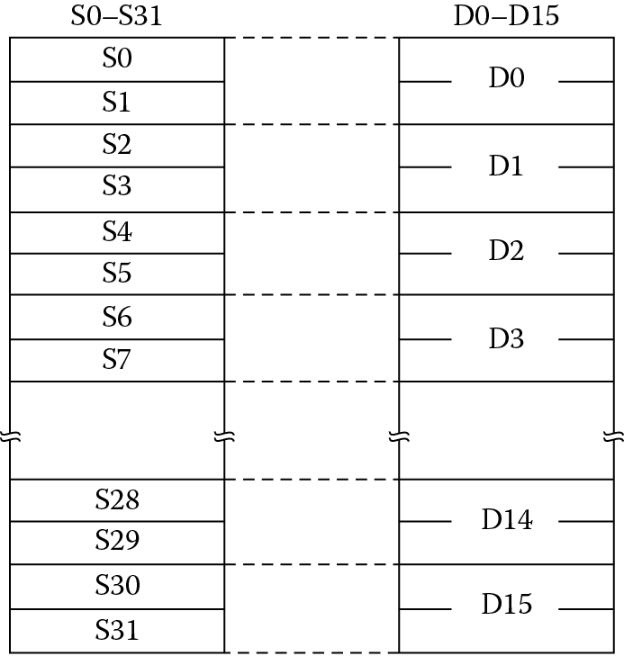
Each single-precision register may be used as a source or destination, or both, in any instruction. There are no limitations on the use of the registers, unlike register r13, register r14, and register r15 in the integer register file. This is referred to as a flat register file, although some restrictions do exist when a standard protocol, such as the ARM Architecture Procedure Call Standard (AAPCS), is in place for passing operands and results to subroutines and functions. The FPU registers are aliased, such that two single-precision registers may be referenced as a double-precision register. The aliasing follows the relation shown below.
For example, register d[6] is aliased to the register pair {s13, s12}. In several of the load and store instructions, the FPU operand may be either a single-precision or double-precision register. This enables 64-bit data transfers with memory and with the ARM register file. It’s important to ensure that you know which single-precision registers are aliased to a double-precision register, so you don’t accidently overwrite a single-precision register with a load to a double-precision register.
9.8 FPU Control Registers
Two control registers are of immediate importance, and they are the FPSCR and the CPACR. The first controls the internal workings of the FPU, while the second enables the FPU. If the FPU is not enabled, any access to the FPU will result in a fault. This will be covered in more detail in Chapter 15, but for now we need to know that the FPU must be enabled or our programs will not work.
9.8.1 The Floating-Point Status and Control Register, FPSCR
In Chapter 7, we became familiar with the various status registers, e.g., the CPSR and APSR. We also examined the use of the register to hold condition code flags and to specify various options and modes of operation. The equivalent register in the FPU is the Floating-Point Status and Control Register (FPSCR), shown in Figure 9.12. Reading and writing the FPSCR is covered in Chapter 11. Notice that the APSR and the FPSCR are alike in that the upper 4 bits hold the status of the last comparison, the N, Z, C, and V bits. These bits record the results of floating-point compare instructions (considered in Chapter 11) and can be transferred to the APSR for use in conditional execution and conditional branching.
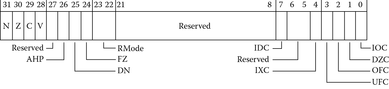
9.8.1.1 The Control and Mode Bits
The bits following the status bits are used to specify modes of operation. The AHP bit specifies the “alternative half-precision format” to select the format of the half-precision data type. If set to zero, the IEEE 754-2008 format is selected, and if set to 1, the ARM alternative format is selected. The DN bit selects whether the FPU is in “default NaN” mode. When not in default NaN mode (the common case), operations with NaN input values preserve the NaN (or one of the NaN values, if more than one input operand is a NaN) as the result. When in default NaN mode any operation involving a NaN returns the default NaN as the result, regardless of the NaN payload or payloads. The default NaN is a qNaN with an all-zero payload, as in Table 9.11.
Format of the Default Nan for Half-Precision and Single-Precision Data Types
|
Format |
||
|
Half-Precision |
Single-Precision |
|
|
Sign bit |
0 |
0 |
|
Exponent |
0x1F |
0xFF |
|
Fraction |
bit [9] = 1, bits [8:0] = 0 |
bit [22] = 1, bits [21:0] = 0 |
The FZ bit selects whether the processor is in flush-to-zero mode. When set, the processor ignores subnormal inputs, replacing them in computations with signed zeroes, and flushes a result in the subnormal range to a signed zero. Both the DN and FZ bits are discussed in greater detail in Chapter 11. Bits 23 and 22 contain the RMode bits. These bits specify the rounding mode to be used in the execution of most operations. The default rounding mode is roundTiesToEven, also known as Round to Nearest Even. It’s important to know where these bits may be found, but we will not take up rounding until Chapter 10. The rounding mode is selected by setting the RMode bits to one of the bit patterns shown in Table 9.12.
Rounding Mode Bits
|
Rounding Mode |
Setting in FPSCR[22:23] |
|
roundTiesToEven |
0b00 (default) |
|
roundTowardPositive |
0b01 |
|
roundTowardNegative |
0b10 |
|
roundTowardZero |
0b11 |
9.8.1.2 The Exception Bits
The status bits in the lower 8 bits of the FPSCR indicate when an exceptional condition has occurred. We will examine exceptions in Chapter 10, but here we only need to know that these bits are set by hardware and cleared only by a reset or a write to the FPSCR. The Cortex-M4 does not trap on any exceptional conditions, so these bits are only useful to the programmer to identify an exceptional condition has occurred since the bit was last cleared.
The exception bits are shown in the Table 9.13. Each of these bits is “sticky”, that is, they are set on the first instance of the condition, and remain set until cleared by a write to the FPSCR. If the bits are cleared before a block of code, they will indicate whether their respective condition occurred in that block. They won’t tell you what instruction or operand(s) caused the condition, only that it occurred somewhere in the block of code. To learn this information more precisely you can step through the code and look for the instruction that set the exception bit of interest.
FPSCR Exception Bits
|
FPSCR Bit Number |
Bit Name |
This Bit Is Set When |
|
7 |
IDC Input Denormal |
An input to an operation was subnormal and was flushed to zero before used in the operation. Valid only in flush-to-zero mode. |
|
4 |
IXC Inexact |
An operation returned a result that was not representable in the single-precision format, and a rounded result was written to the register file. |
|
3 |
UFC Underflow |
An operation returned a result that, in absolute value, was smaller in magnitude than the positive minimum normalized number before rounding , and was not exact. |
|
2 |
OFC Overflow |
An operation returned a result that, in absolute value, was greater in magnitude than the positive maximum number after rounding . |
|
1 |
DZC Division by Zero |
A divide had a zero divisor and the dividend was not zero, an infinity or a NaN. |
|
0 |
IOC Invalid Operation |
An operation has no mathematical value or cannot be represented. |
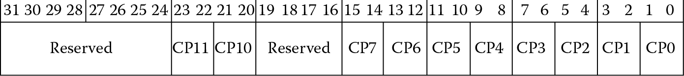
9.8.2 The Coprocessor Access Control Register, CPACR
The Coprocessor Access and Control Register, known as the CPACR, controls the access rights to all implemented coprocessors, including the FPU. Coprocessors are addressed by coprocessor number, a four-bit field in coprocessor instructions that identifies to the coprocessor whether it is to handle this instruction or to ignore it. Coprocessors are identified by CPn, where n is a number from 0 to 15. Coprocessors CP8 to CP15 are reserved by ARM, allowing system-on-chip designers to utilize CP0-CP7 for special function devices that can be addressed by coprocessor instructions. ARM processors have supported user coprocessors from the ARM1, but designing and incorporating custom coprocessors is not a trivial exercise, and is beyond the scope of this book. The FPU in ARM processors uses coprocessor numbers CP10 and CP11. The two coprocessor numbers are part of each FPU instruction, and specify the precision of the instruction, with CP10 specifying single-precision execution and CP11 specifying double-precision execution. Since the Cortex-M4 executes instructions operating on single-precision operands only, CP10 must be enabled. However, some of the instructions which load and store 64-bit double-precision data are in CP11 space, so it makes sense to enable both CP10 and CP11.
To enable the FPU the two bits corresponding to CP10 and CP11, bits 23:22 and 21:20, must be set to either 01 or 11. If CP10 and CP11 are each set to 01, the FPU may be accessed only in a privileged mode. If code operating in unprivileged Thread mode attempts to execute a FPU instruction, a UsageFault will be triggered and execution will transfer to a handler routine. For more information on exceptions and exception handling, see Chapter 15. If the bits are set to 11, the FPU is enabled for operations in privileged and unprivileged modes. This is the mode in which we will operate for our examples, but if you were designing a system you would have the flexibility to utilize the privileged and unprivileged options in your system code. The format of the CPACR is shown in Figure 9.13.
The following code may be used to enable CP10 and CP11 functionality in both privileged and unprivileged modes. The CPACR is a memory-mapped register, that is, it is addressed by a memory address rather than by a register number. In the Cortex-M4 the CPACR is located at address 0xE000ED88.
; Enable the FPU, both CP10 and CP11, for
; privileged and unprivileged mode accesses
; CPACR is located at address 0xE000ED88
LDR.W r0, = 0xE000ED88
; Read CPACR
LDR r1, [r0]
; Set bits 20-23 to enable CP10 and CP11 coprocessors
ORR r1, r1, #(0xF << 20)
; Write back the modified value to the CPACR
STR r1, [r0]
; Wait for store to complete
DSB
It is necessary to execute this code or some code that performs the same functions before executing any code that loads data into the FPU or executes any FPU operations.
9.9 Loading Data into Floating-Point Registers
We have seen the various data types and formats available in the Cortex-M4 FPU, but how is data loaded into the register file and stored to memory? Fortunately, the instructions for loading and storing data to the FPU registers share features with the integer instructions seen in Chapter 5. We will first consider transfers to and from memory, then with the integer register file, and finally between FPU registers.
9.9.1 Floating-Point Loads and Stores: The Instructions
Memory is accessed in the same way for floating-point data and integer data. The instructions and the format for floating-point loads and stores is given below.
VLDR|VSTR{<cond>}.32 <Sd>, [<Rn>{, #+/ − <imm>}]
VLDR|VSTR{<cond>}.64 <Dd>, [<Rn>{, #+/ − <imm>}]
The <cond> is an optional condition field, as discussed in Chapter 8. Notice that these instructions do not follow the convention of naming the destination first. For both loads and stores the FPU register is named first and the addressing follows. All FPU instructions may be predicated by a condition field; however, as described in Chapter 8, selecting a predicate, such as NE, introduces an IT instruction to affect the predicated execution. The <Sd> value is a single-precision register, the <Dd> register is a pair of single-precision registers, the <Rn> register is an integer register, and the <imm> field is an 8-bit signed offset field. This addressing mode is referred to as pre-indexed addressing, since the offset is added to the address in the index register to form the effective address. For example, the instruction
VLDR s5, [r6, #08]
loads the 32-bit value located in memory into FPU register s5. The address is created from the value in register r6 plus the offset value of 8. Only fixed offsets and a single-index register are available in the FPU load and store instructions. An offset from an index register is useful in accessing constant tables and stacked data. Stacks will be covered in Chapter 13, and we will see an example of floating-point tables in Chapter 12.
VLDR may also be used to create literal pools of constants. This use is referred to as a pseudo-instruction, meaning the instruction as written in the source file is not a valid Cortex-M4 instruction, but is used by the assembler as a shortcut. The VLDR pseudo-instruction used with immediate data creates a constant table and generates VLDR PC-relative addressed instructions. The format of the instruction is:
VLDR{<cond>}.F32 Sd, =constant
VLDR{<cond>}.F64 Dd, =constant
Any value representable by the precision of the register to be loaded may be used as the constant. The format of the constants in the Keil tools may be any of the following:
[+/−]number.number (e.g., −5.873, 1034.77)
[+/−]number[e[+/−]number] (e.g., 6e-5, −123e12)
[+/−]number.number[e[+/−]number] (e.g., 1.25e-18, −5.77e8)
For example, to load Avogadro’s constant, the molar gas constant, and Boltzmann’s constant in single-precision, the following pseudo-instructions are used to create a literal pool and generate the VLDR instructions to load the constant into the destination registers.
VLDR.F32 s14, =6.0221415e23 ; Avogadro’s number
VLDR.F32 s15, =8.314462 ; molar gas constant
VLDR.F32 s16, =1.3806505e-23 ; Boltzmann’s constant
The following code is generated:
41: VLDR.F32 s14, = 6.0221415e23 ; Avogadro’s number
0x0000001C ED9F7A03 VLDR s14,[pc,#0x0C]
42: VLDR.F32 s15, = 8.314462 ; molar gas constant
0x00000020 EDDF7A03 VLDR s15,[pc,#0x0C]
43: VLDR.F32 s16, = 1.3806505e-23 ; Boltzmann’s constant
0x00000024 ED9F8A03 VLDR s16,[pc,#0x0C]
The memory would be populated as shown below.
0x0000002C 0C30 DCW 0x0C30
0x0000002E 66FF DCW 0x66FF
0x00000030 0814 DCW 0x0809
0x00000032 4105 DCW 0x4105
0x00000034 8740 DCW 0x8740
0x00000036 1985 DCW 0x1985
You should convince yourself these constants and offsets are correct.
For hexadecimal constants, the following may be used:
VLDR{<cond>}.F32 Sd, =0f_xxxxxxxx
where xxxxxxxx is an 8 character hex constant. For example,
VLDR.F32 s17, =0f_7FC00000
will load the default NaN value into register s17.
Note that Code Composer Studio does not support VLDR pseudo-instructions. See Section 6.3.
9.9.2 The VMOV instruction
Often we want to copy data between ARM registers and the FPU. The VMOV instruction handles this, along with moving data between FPU registers and loading constants into FPU registers. The first of these instructions transfers a 32-bit operand between an ARM register and an FPU register; the second between an FPU register and an ARM register:
VMOV{<cond>}.F32 <Sd>, <Rt>
VMOV{<cond>}.F32 <Rt>, <Sn>
The format of the data type is given in the .F32 extension. When it could be unclear which data format the instruction is transferring, the data type is required to be included. The data type may be one of the following shown in Table 9.14.
Data Type Identifiers
|
Data Type |
Identifier |
|
Half-precision |
.F16 |
|
Single-precision |
.F32 or .F |
|
Double-precision |
.F64 or .D |
We referred to the operand simply as a 32-bit operand because what is contained in the source register could be any 32-bit value, not necessarily a single-precision operand. For example, it could contain two half-precision operands. However, it does not have to be a floating-point operand at all. The FPU registers could be used as temporary storage for any 32-bit quantity.
The VMOV instruction may also be used to transfer data between FPU registers. The syntax is
VMOV{<cond>}.F32 <Sd>, <Sn>
One important thing to remember in any data transfer operation is that the content of the source register is ignored in the transfer. That is, the data is simply transferred bit by bit. This means that if the data in the source register is an sNaN, the IOC flag will not be set. This is true for any data transfer operation, whether between FPU registers, or between an FPU register and memory, or between an FPU register and an ARM register.
As a legacy of the earlier FPUs that processed double-precision operands, the following VMOV instructions transfer to or from an ARM register and the upper or lower half of a double-precision register. The x is replaced with either a 1, for the top half, or a 0, for the lower half. This is necessary to identify which half of the double-precision register is being transferred.
VMOV{<cond>}.F32 <Dd[x]>, <Rt>
VMOV{<cond>}.F32 <Rt>, <Dn[x]>
It is not necessary to include the .F32 in the instruction format above, but it is good practice to make the data type explicit whenever possible. The use of this form of the VMOV instruction is common in routines which process double-precision values using integer instructions, such as routines that emulate double-precision operations. You may have access to integer routines that emulate the double-precision instructions that are defined in the IEEE 754-2008 specification but are not implemented in the Cortex-M4.
Two sets of instructions allow moving data between two ARM registers and two FPU registers. One key thing to note is that the ARM registers may be independently specified but the FPU registers must be contiguous. As with the instructions above, these are useful in handling double-precision operands or simply moving two 32-bit quantities in a single instruction. The first set is written as
VMOV{<cond>} <Sm>, <Sm1>, <Rt>, <Rt2>
VMOV{<cond>} <Rt>, <Rt2>, <Sm>, <Sm1>
The transfer is always between Sm and Rt, and Sm1 and Rt2. Sm1 must be the next contiguous register from Sm, so if Sm is register s6 then Sm1 is register s7. For example, the following instruction
VMOV s12, s13, r6, r11
would copy the contents of register r6 into register s12 and register r11 into register s13. The reverse operation is also available. The second set of instructions substitutes the two single-precision registers with a reference to a double-precision register. This form is a bit more limiting than the instructions above, but is often more useful in double-precision emulation code. The syntax for these instructions is shown below.
VMOV{<cond>} <Dm>, <Rt>, <Rt2>
VMOV{<cond>} <Rt>, <Rt2>, <Dm>
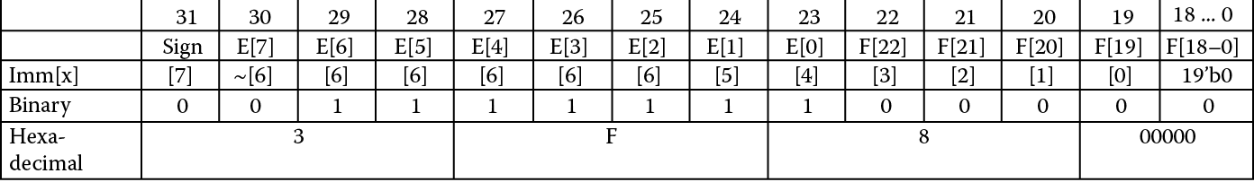
One final VMOV instruction is often very useful when a simple constant is needed. This is the immediate form of the instruction,
VMOV{<cond>}.F32 <Sd>, #<imm>
For many constants, the VMOV immediate form loads the constant without a memory access. Forming the constant can be a bit tricky, but fortunately for us, the assembler will do the heavy lifting. The format of the instruction contains two immediate fields, imm4H and imm4L, as we see in Figure 9.14.

The destination must be a single-precision register, meaning this instruction cannot be used to create half-precision constants. It’s unusual for the programmer to need to determine whether the constant can be represented, but if code space or speed is an issue, using immediate constants saves on area and executes faster than the PC-relative loads generated by the VLDR pseudo-instruction.
The single-precision operand is formed from the eight bits contained in the two 4-bit fields, imm4H and imm4L. The imm4H contains bits 7-4, and imm4L bits 3-0. The bits contribute to the constant as shown in Figure 9.15.

While at first glance this does look quite confusing, many of the more common constants can be formed this way. The range of available constants is
+/− (1.0 … 1.9375) × 2(−3 … +4)
For example, the constant 1.0, or 0x3F800000, is formed when the immediate field is imm4H = 0111 and imm4L = 0000. When these bits are inserted as shown in Figure 9.15, we have the bit pattern shown in Figure 9.16.
Some other useful constants suitable for the immediate VMOV include those listed in Table 9.15. Notice that 0 and infinity cannot be represented, and if the constant cannot be constructed by this instruction, the assembler will create a literal pool.
Useful Floating-Point Constants
|
Constant Value |
imm4H |
Imm4L |
|
0.5 |
0110 |
0000 |
|
0.125 |
0100 |
0000 |
|
2.0 |
0000 |
0000 |
|
31 |
0011 |
1111 |
|
15 |
0010 |
1110 |
|
4.0 |
0001 |
0000 |
|
−4.0 |
1001 |
0000 |
|
1.5 |
0111 |
1000 |
|
2.5 |
0001 |
0100 |
|
0.75 |
0110 |
1000 |
9.10 Conversions between Half-Precision and Single-Precision
A good way to reduce the memory usage in a design is to use the smallest format that will provide sufficient range and precision for the data. As we saw in Section 9.6.1, the half-precision data type has a range of +/− 6.10 × 10⁻⁵ to +/− 6.55 × 10⁴, with 10 fraction bits, giving roughly 3.3 digits of precision. When the data can be represented in this format, only half the memory is required as compared to using single-precision data for storage.
The instructions VCVTB and VCVTT convert a half-precision value in either the lower half or upper half of a floating-point register, respectively, to a single-precision value, or convert a single-precision value to a half-precision value and store it in either the lower half or upper half of the destination floating-point register. The syntax of these instructions is
VCVTB{<cond>}.F32.F16 <Sd>, <Sm>
VCVTT{<cond>}.F32.F16 <Sd>, <Sm>
VCVTB{<cond>}.F16.F32 <Sd>, <Sm>
VCVTT{<cond>}.F16.F32 <Sd>, <Sm>
The B variants operate on the lower 16 bits of the Sm or Sd register, while the T variants operate on the upper 16 bits. These instructions provide a means of storing table data that does not require the precision or range of single-precision floating-point but can be represented sufficiently in the half-precision format.
9.11 Conversions to Non-Floating-Point Formats
Often data is input to a system in integer or fixed-point formats and must be converted to floating-point to be operated on. For example, the analog-to-digital converter in the TM4C1233H6PM microcontroller from Texas Instruments outputs a 12-bit digital conversion in the range 0 to the analog supply voltage, to a maximum of 4 volts. Using the fixed-point to floating-point conversion instructions, the conversion from a converter output to floating-point is possible in two instructions—one to move the data from memory to a floating-point register, and the second to perform the conversion. The range of options in the fixed-point conversion instructions makes it easy to configure most conversions without any scaling required. In Chapter 18, we will look at how to construct conversion routines using these instructions, which may be easily called from C or C++.
In the following sections, we will look at the instructions for conversion between 32-bit integers and floating-point single-precision, and between 32-bit and 16-bit fixed-point and floating-point single-precision.
9.11.1 Conversions between Integer and Floating-Point
The Cortex-M4 has two instructions for conversion between integer and floating-point formats. The instructions have the format
VCVT{R}<c>.<T32>.F32 <Sd>, <Sm>
VCVT<c>.F32.<T32> <Sd>, <Sm>
The <T32> may be replaced by either S32, for 32-bit signed integer, or U32, for 32-bit unsigned integer. Conversions to integer format commonly use the roundTowardZero (RZ) format. This is the behavior seen in the C and C++ languages; conversion of a floating-point value to an integer always truncates any fractional part. For example, each of the following floating-point values, 12.0, 12.1, 12.5, and 12.9, will return 12 when converted to integer. Likewise, −12.0, −12.1, −12.5, and −12.9 will return −12. To change this behavior, the R variant may be used to perform the conversion using the rounding mode in the FPSCR. When the floating-point value is too large to fit in the destination precision, or is an infinity or a NaN, an Invalid Operation exception is signaled, and the largest value for the destination type is returned. Exceptions are covered in greater detail in Chapter 10.
A conversion from integer to floating-point always uses the rounding mode in the FPSCR. If the conversion is not exact, as in the case of a very large integer that has more bits of precision than are available in the single-precision format, the Inexact exception is signaled, and the input integer is rounded. For example, the value 10,000,001 cannot be precisely represented in floating-point format, and when converted to single-precision floating-point will signal the Inexact exception.
9.11.2 Conversions between Fixed-Point and Floating-Point
The formats of the fixed-point data type in the Cortex-M4 can be either 16 bits or 32 bits, and each may be signed or unsigned. The position of the binary point is identified by the <fbits> field, which specifies the number of fractional bits in the format. For example, let us specify an unsigned, 16-bit, fixed-point format in which there are 8 bits of integer data and 8 bits of fractional data. So the range of this data type is [0, 128), with a numeric separation of 1/256, or 0.00390625. That is, the value increments by 1/256 as one is added to the least-significant bit.
The instructions have the format
VCVT{<cond>}.<Td>.F32 <Sd>, <Sd>, #<fbits>
VCVT{<cond>}.F32.<Td> <Sd>, <Sd>, #<fbits>
The <Td> value is the format of the fixed-point value, one of U16, S16, U32, or S32. Rounding of the conversions depends on the direction. Conversions from fixed-point to floating-point are always done with the roundTiesToEven rounding mode, and conversions from floating-point to fixed-point use the roundTowardZero rounding mode. We will consider these rounding modes in Chapter 10. One thing to notice in these instructions is the reuse of the source register for the destination register. This is due to the immediate <fbits> field. Simply put, there is not room in the instruction word for two registers, so the source register is overwritten. This should not be an issue; typically this instruction takes a fixed-point value and converts it, and the fixed-point value is needed only for the conversion. Likewise, when a floating-point value is converted to a fixed-point value, the need for the floating-point value is often gone.
Example 9.5
Convert the 16-bit value 0x0180 in U16 format with 8 bits of fraction to a single-precision floating-point value.
Solution
ADR r1, DataStore
LDRH r2, [r1]
; Convert each of the 16-bit data to single-precision with
; different <fbits> values
VMOV.U16 s7, r2 ; load the 16-bit fixed-pt to s reg
VCVT.F32.U16 s7, s7, #8 ; convert the fixed-pt to SP with
; 8 bits of fraction
loop B loop
ALIGN
DataStore
DCW 0x0180
The value in register s7 after this code is run is 0x3FC00000, which is 1.5. How did the Cortex-M4 get this value? Look at Table 9.16.
Output of Example 9.5
|
Format U/S, <fbits > |
Hex Value |
Binary Value |
Decimal Value |
Single-Precision Floating-Point Value |
|
U16, 8 |
0x0180 |
00000001.10000000 |
1.5 |
0x3FC00000 |
Notice that we specified 8 bits of fraction (here 8’b10000000, representing 0.5 in decimal) and 8 bits of integer (here 8’b00000001, representing 1.0), hence the final value of 1.5. In this format, the smallest representable value would be 0x0001 and would have the value 0.00390625, and the largest value would be 0xFFFF, which is 255.99609375 (256 – 0.00390625). Any multiple of 0.00390625 between these two values may be represented in 16 bits. If we wanted to do this in single-precision, each value would require 32 bits. With the U16 format we can represent each in only 16 bits.
There are valid uses for this type of conversion. The cost of memory is often a factor in the cost of the system, and minimizing memory usage, particularly ROM storage, will help. Another use is generating values that may be used by peripherals that expect outputs in a non-integer range. If we want to control a motor and the motor control inputs are between 0 to almost 10, with 4 bits of fraction (so we can increment by 1/16, i.e., 0, 1/16, 1/8, 3/16, … 9.8125, 9.875) the same instruction can be used to convert from floating-point values to U16 values. Conversion instructions are another tool in your toolbox for optimizing your code for speed or size, and in some cases, both.
The 16-bit formats may also be interpreted as signed when the S16 format is used, and both signed and unsigned fixed-point 32-bit values are available. Table 9.17 shows how adjusting the #fbits value can change how a 16-bit hex value is interpreted. If the #fbits value is 0, the 16 bits are interpreted as an integer, either signed or unsigned, and the numeric separation is 1, as we expect in the integer world. However, if we choose #fbits to be 8, the 16 bits are interpreted as having 8 integer bits and 8 fraction bits, and the range is that of an 8-bit integer, but with a numeric separation of 2−8, or 0.00390625, allowing for a much higher precision than is available with integers by trading off range.
Ranges of Available 16-Bit Fixed-Point Format Data
|
fbits |
Integer Bits: Fraction Bits |
Numeric Separation |
Range Unsigned Range Signed |
|
0 |
16:0 |
20 , 1 |
0 … 65,535 − 32,768 … 32,767 |
|
1 |
15:1 |
2− 1 , 0.5 |
0 … 32,767.5 − 16,384 … 16,383.5 |
|
2 |
14:2 |
2− 2 , 0.25 |
0 … 16,383.75 − 8,192 … 8,191.75 |
|
3 |
13:3 |
2− 3 , 0.125 |
0 … 8,191.875 − 4,096 … 4,047.875 |
|
4 |
12:4 |
2− 4 , 0.0625 |
0 … 4,095.9375 − 2,048 … 2,023.9375 |
|
5 |
11:5 |
2− 5 , 0.03125 |
0 … 2,047.96875 − 1,024 … 1,023.96875 |
|
6 |
10:6 |
2− 6 , 0.015625 |
0 … 1,023.984375 − 512 … 511.984375 |
|
7 |
9:7 |
2− 7 , 0.0078125 |
0 … 511.9921875 − 256 … 255.9921875 |
|
8 |
8:8 |
2− 8 , 0.00390625 |
0 … 255.99609375 − 128 … 127.99609375 |
|
9 |
7:9 |
2− 9 , 0.001953125 |
0 … 127.998046875 − 64 … 63.998046875 |
|
10 |
6:10 |
2− 10 , 0.000976563 |
0 … 63.999023438 − 32 … 31.999023438 |
|
11 |
5:11 |
2− 11 , 0.000488281 |
0 … 31.99951171875 − 16 … 15.99951171875 |
|
12 |
4:12 |
2− 12 , 0.000244141 |
0 … 15.999755859375 − 8 … 7.999755859375 |
|
13 |
3:13 |
2− 13 , 0.00012207 |
0 … 7.9998779296875 4 … 3.9998779296875 |
|
14 |
2:14 |
2− 14 , 6.10352E-05 |
0 … 3.99993896484375 2 … 1.99993896484375 |
|
15 |
1:15 |
2− 15 , 3.05176E-05 |
0 … 1.999969482421875 − 1 … 0.999969482421875 |
|
16 |
0:16 |
2− 16 , 1.52588E-05 |
0 … 0.999984741210937 − 0.5 … 0.499984741210937 |
When the range and desired precision are known, for example, for a sensor attached to an analog-to-digital converter (ADC) or for a variable speed motor, the fixed-point format can be used to input the data directly from the converter without having to write a conversion routine. For example, if we have an ADC with 16-bit resolution over the range 0 to +VREF, we could choose a VREF value of 4.0 V. The U16 format with 14 fraction bits has a range of 0 up to 4 with a resolution of 2−14. All control computations for the motor control could be made using a single-precision floating-point format and directly converted to a control voltage using
VCVT.U16.F32 s9, s9, #14
The word value in the s9 register could then be written directly to the ADC buffer location in the memory map. If the conversion is not 16 bits, but say 12 bits, conversion with the input value specified to be the format U16 with 10 fraction bits would return a value in the range 0 to 4 for all 12-bit inputs. Similarly, if VREF is set to 2 V, the U16 format with 15 fraction bits would suffice for 16-bit inputs and the U16 with 11 fraction bits for 12-bit inputs. The aim of these instructions is to eliminate the need for a multiplier step for each input sampled or control output. Careful selection of the VREF and the format is all that is required. Given the choice of signed and unsigned formats and the range of options available, these conversion instructions can be a powerful tool when working with physical input and output devices.
9.12 Exercises
- Represent the following values in half-precision, single-precision, and double-precision.
- 1.5
- 3.0
- −4.5
- −0.46875
- 129
- −32768
- Write a program in a high-level language to take as input a value in the form (−)x.y and convert the value to single-precision and double-precision values.
- Using the program from Exercise 2 (or a converter on the internet), convert the following values to single-precision and double-precision.
- 65489
- 2147483648
- 229
- −0.38845
- 0.0004529
- 11406
- −57330.67
- Expand the program in Exercise 2 to output half-precision values. Test your output on the values from Exercise 3. Which would fit in half-precision?
- Write a program in a high-level language to take as input a single-precision value in the form 0xXXXXXXXX (where X is a hexadecimal value) and convert the input to decimal.
- Using the program from Exercise 5 (or a converter on the internet), convert the following single-precision values to decimal. Identify the class of value for each input. If the input is a NaN, give the payload as the value, and NaN type in the class field.
Single-Precision Value
Value
Class
a. 0x3fc00000
b. 0x807345ff
c. 0x7f350000
d. 0xffffffff
e. 0x20000000
f. 0x7f800000
g. 0xff800ffe
h. 0x42c80000
i. 0x4d800000
j. 0x80000000
- What value would you write to the FPSCR to set the following conditions?
- FZ unset, DN unset, roundTowardZero rounding mode
- FZ set, DN unset, roundTowardPositive rounding mode
- FZ set, DN set, roundTiesToEven rounding mode
- Complete the following table for each of the FPSCR values shown below.
N
Z
C
V
DN
FZ
RMode
IDC
IXC
UFC
OFC
DZC
IOC
0x41c00010
0x10000001
0xc2800014
- Give the instructions to load the following values to FPU register s3.
- 5.75 × 10³
- 147.225
- –9475.376
- −100.6 × 10⁻⁸
- Give the instructions to perform the following load and store operations.
- Load the 32-bit single-precision value at the address in register r4 into register s12.
- Load the 32-bit single-precision value in register r6 to register s12. Repeat for a store of the value in register s15 to register r6.
- Store the 32-bit value in register s4 to memory at the address in register r8 with an offset of 16 bytes.
- Store the 32-bit constant 0xffffffff to register s28.
- Give the instructions to perform a conversion of four fixed-point data in unsigned 8.8 format stored in register s8 to register s11 to single-precision format.
- What instruction would you use to convert a half-precision value in the lower half of register s5 to a single-precision value, and store the result in register s2?
- Give the instructions to load 8 single-precision values at address 0x40000100 to FPU registers s8 to s15.
- How many subnormal values are there in a single-precision representation? Is this the same number as values for any non-zero exponent?
* Konrad Zuse’s Legacy: The architecture of the Z1 and Z3, IEEE Annals of the History of Computing, 19, 2, 1997, pp. 5–16.
†* See IBM System/360 Principles of Operation, IBM File No. S360-01, pp. 41–42, available from http://bitsavers.informatik.uni-stuttgart.de/pdf/ibm/360/princOps/A22-6821-6_360PrincOpsJan67.pdf.
‡* We will consider values, or encodings, for values that are not in the space of normal values in Section 9.6.
§ The ARM documentation in the ARM v7-M Architecture Reference Manual uses the terms “denormal” and “denormalized” to refer to subnormal values. The ARM Cortex-M4 Technical Reference Manual uses the terms “denormal” and “subnormal” to refer to subnormal values.
¶ In some rounding modes, a value of Maximum Normal will be returned. We will consider this case in the section in our discussion of exceptions.
** Buick is a brand of General Motors vehicle popular in the 1980s.