Chapter 3

Introduction to Instruction Sets

v4T and v7-M

3.1 Introduction

This chapter introduces basic program structure and a few easy instructions to show how directives and code create an assembly program. What are directives? How is the code stored in memory? What is memory? It’s unfortunate that the tools and the mechanics of writing assembly have to be learned simultaneously. Without software tools, the best assembly ever written is virtually useless, difficult to simulate in your head, and even harder to debug. You might find reading sections with unfamiliar instructions while using new tools akin to learning to swim by being thrown into a pool. It is. However, after going through the exercise of running a short block of code, the remaining chapters take time to look at all of the details: directives, memory, arithmetic, and putting it all together. This chapter is meant to provide a gentle introduction to the concepts behind, and rules for writing, assembly programs.

First, we need tools. While the ideas behind assemblers haven’t changed over the years, the way that programmers work with an assembler has, in that command-line assemblers aren’t really the first tool that you want to use. Integrated Development Environments (IDEs) have made learning assembly much easier, as the assembler can be driven graphically. Gone are the days of having paper tape as an input to the machine, punch cards have been relegated to museums, and errors are reported in milliseconds instead of hours. More importantly, the countless options available with command-line assemblers are difficult to remember, so our introduction starts the easy way, graphically. Graphical user interfaces display not only the source code, but memory, registers, flags, the binary listings, and assembler output all at once. Tools such as the Keil MDK and Code Composer Studio will set up most of the essential parameters for us.

If you haven’t already installed and familiarized yourself with the tools you plan to use, you should do so now. By using tools that support integrated development, such as those from Keil, ARM, IAR, and Texas Instruments, you can enter, assemble, and test your code all in the same environment. Refer to Appendices A and B for instructions on creating new projects and running the code samples in the book. You may also choose to use other tools, either open-source (like gnu) or commercial, but note there might be subtle changes to the syntax presented throughout this book, and you will want to consult your software’s documentation for those details. Either way, today’s tools are vastly more helpful than those used 20 years ago—no clumsy breakpoint exceptions are needed; debugging aids are already provided; and everything is visual!

3.2 ARM, Thumb, and Thumb-2 Instructions

There is no clean way to avoid the subject of instruction length once you begin writing code, since the instructions chosen for your program will depend on the processor. Even more daunting, there are options on the length of the instruction—you can choose a 32-bit instruction or let the assembler optimize it for you if a smaller one exists. So some background on the instructions themselves will guide us in making sense of these differences. ARM instructions are 32 bits wide, and they were the first to be used on older architectures such as the ARM7TDMI, ARM9, ARM10, and ARM11. Thumb instructions, which are a subset of ARM instructions, also work on 32-bit data; however, they are 16 bits wide. For example, adding two 32-bit numbers together can be done one of two ways:

ARM instruction ADD r0, r0, r2

Thumb instruction ADD r0, r2

The first example takes registers r0 and r2, adds them together, then stores the result back in register r0. The data contained in those registers as well as the ARM instruction itself is 32 bits wide. The second example does the exact same thing, only the instruction is 16 bits wide. Notice there are only two operands in the second example, so one of the operands, register r0, acts as both the source and destination of the data. Thumb instructions are supported in older processors such as the ARM7TDMI, ARM9, and ARM11, and all of the Cortex-A and Cortex-R families.

Thumb-2 is a superset of Thumb instructions, including new 32-bit instructions for more complex operations. In other words, Thumb-2 is a combination of both 16-bit and 32-bit instructions. Generally, it is left to the compiler or assembler to choose the optimal size, but a programmer can force the issue if necessary. Some cores, such as the Cortex-M3 and M4, only execute Thumb-2 instructions—there are no ARM instructions at all. The good news is that Thumb-2 code looks very similar to ARM code, so the Cortex-M4 examples below resemble those for the ARM7TDMI, allowing us to concentrate more on getting code to actually run. In Chapter 17, Thumb and Thumb-2 are discussed in detail, especially in the context of optimizing code, but for now, only a few basic operations will be needed.

3.3 Program 1: Shifting Data

Finally, we get around to writing up and describing a real, albeit small, program using a few simple instructions, some directives, and the tools to watch everything in action. The code below takes a simple value (0x11), loads it into a register, and then shifts it one bit to the left, twice. The code could be written identically for either the Cortex-M4 or an ARM7TDMI, but we’ll look at the first example using only the ARM7TDMI using Keil directives, shown below.

	AREA Prog1, CODE, READONLY

	ENTRY

	MOV	r0, #0x11	; load initial value

	LSL	r1, r0, #1	; shift 1 bit left

	LSL	r2, r1, #1	; shift 1 bit left

stop	B	stop		; stop program

	END

For the assembler to create a block of code, we need the AREA declaration, along with the type of data we have—in this case, we are creating instructions, not just data (hence the CODE option), and we specify the block to be read-only. Since all programs need at least one ENTRY declaration, we place it in the only file that we have, with the only section of code that we have. The only other directive we have for the assembler in this file is the END statement, which is needed to tell the assembler there are no further instructions beyond the B (branch) instruction.

For most of the instructions (there are a few exceptions), the general format is

instruction destination, source, source

with data going from the source to the destination. Our first MOV instruction has register r0 as its destination register, with an immediate value, a hex number, as the source operand. We’ll find throughout the book that instructions have a variety of source types, including numbers, registers, registers with a shift or rotate, etc. The MOV command is normally used to shuffle data from one register to another register. It is not used to load data from external memory into a register, and we will see that there are dedicated load and store instructions for doing that. The LSL instruction takes the value in register r0, shifts it one bit to the left, and moves the result to register r1. In Chapter 6, we will look at the datapaths of the ARM7TDMI and the Cortex-M4 in more detail, but for now, note that we can also modify other instructions for performing simple shifts, such as an ADD, using two registers as the source operands in the instruction, and then providing a shift count. The second LSL instruction is the same as the first, shifting the value of register r1 one bit to the left and moving the result to register r2. We expect to have the values 0x11, 0x22, and 0x44 in registers r0, r1, and r2, respectively, after the program completes.

The last instruction in the program tells the processor to branch to the branch instruction itself, which puts the code into an infinite loop. This is hardly a graceful exit from a program, but for the purpose of trying out code, it allows us to terminate the simulation easily by choosing Start/Stop Debug Session from the Debug menu or clicking the Halt button in our tools.

3.3.1 Running the Code

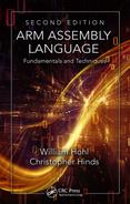
Learning assembly requires an adventurous programmer, so you should try each code sample (and write your own). The best way to hone your skills is to assemble and run these short routines, study their effects on registers and memory, and make improvements as needed. Following the examples provided in Appendices A and B, create a project and a new assembly file. You may wish to choose a simple microcontroller, such as the LPC2104 from NXP, as your ARM7TDMI target, and the TM4C1233H6PM from TI as your Cortex-M4 target (NB: this part is listed as LM4F120H5QR in the Keil tools). Once you’ve started the debugger, you can single-step through the code, executing one instruction at a time until you come to the last instruction (the branch). You may also wish to view the assembly listing as it appears in memory. If you’re using the MDK tools, choose Disassembly Window from the View menu, and your code will appear as in Figure 3.1. You can see the mnemonics in the sample program alongside their equivalent binary representations. Code Composer Studio has a similar Disassembly window, found in its View menu.

Recall from Chapter 1 that a stored program computer holds instructions in memory, and in this first exercise for the ARM7TDMI, memory begins at address 0x00000000 and the last instruction of our program can be found at address 0x0000000C. Notice that the branch instruction at this address has been changed, and that our label called stop has been replaced with its numerical equivalent, so that the line reads

0x0000000C EAFFFFFE B 0x0000000C

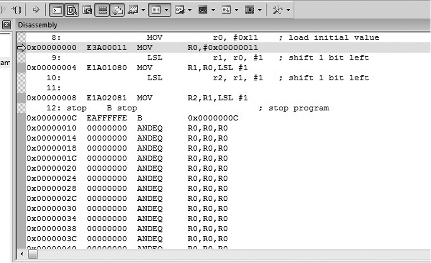
The label stop in this case is the address of the B instruction, which is 0x0000000C. In Chapter 8, we’ll explore how branches work in detail, but it’s worth noting here that the mnemonic has been translated into the binary number 0xEAFFFFFE. Referring to Figure 3.2 we can see that a 32-bit (ARM) branch instruction consists of four bits to indicate the instruction itself, bits 24 to 27, along with twenty-four bits to be used as an offset. When a program uses the B instruction to jump or branch to some new place in memory, it uses the Program Counter to create an address. For our case, the Program Counter contains the value 0x00000014 when the branch instruction is in the execute stage of the ARM7TDMI’s pipeline. Remember that the Program Counter points to the address of the instruction being fetched, not executed. Our branch instruction sits at address 0x0000000C, and in order to create this address, the machine needs merely to subtract 8 from the Program Counter. It turns out that the branch instruction takes its twenty-four-bit offset and shifts it two bits to the left first, effectively multiplying the value by four. Therefore, the two’s complement representation of −2, which is 0xFFFFFE, is placed in the instruction, producing a binary encoding of 0xEAFFFFFE.

Examining memory beyond our small program shows a seemingly endless series of ANDEQ instructions. A quick examination of the bit pattern with all bits clear will show that this translates into the AND instruction. The source and destination registers are register r0, and the conditional field, to be explained in Chapter 8, translates to “if equal to zero.” The processor will fetch these instructions but never execute them, since the branch instruction will always force the processor to jump back to itself.

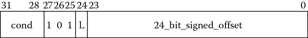
3.3.2 Examining Register and Memory Contents

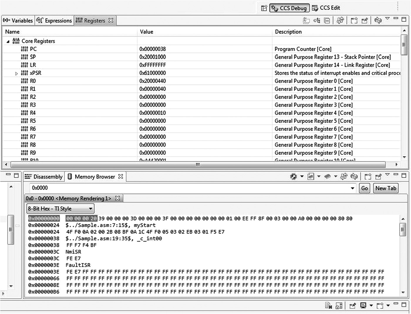
Again referring back to the stored program computer in Chapter 1, we know that both registers and memory can hold data. While you write and debug code, it can be extremely helpful to monitor the changes that occur to registers and memory contents. The upper left-hand corner of Figure 3.3 shows the register window in the Keil tools, where the entire register bank can be viewed and altered. Changing values during debugging sessions can often save time, especially if you just want to test the effect of a single instruction on data. The lower right-hand corner of Figure 3.3 shows a memory window that will display the contents of memory locations given a starting address. Code Composer Studio has these windows, too, shown in Figure 3.4. For now, just note that our ARM7TDMI program starts at address 0x00000000 in memory, and the instructions can be seen in the following 16 bytes. For the next few chapters, we’ll see examples of moving data to and from memory before unleashing all the details about memory in Chapter 5.

Breakpoints can also be quite useful for debugging purposes. A breakpoint is an instruction that has been tagged in such a way that the processor stops just before its execution. To set a breakpoint on an instruction, simply double-click the instruction in the gray bar area. You can use either the source window or the disassembly window. You should notice a red box beside the breakpointed instruction. When you run your code, the processor will stop automatically upon hitting the breakpoint. For larger programs, when you need to examine memory and register contents, set a breakpoint at strategic points in the code, especially in areas where you want to single-step through complex instruction sequences.

3.4 Program 2: Factorial Calculation

The next simple programs we look at for both the ARM7TDMI and the Cortex-M4 are ones that calculate the value of n!, which is a relatively short loop using only a few instructions. Recall that n! is defined as

$n!={\displaystyle \prod _{i=1}^{n}i=n(n-1)(n-2)}...(1)$

For a given value of n, the algorithm iteratively multiplies a current product by a number that is one less than the number it used in the previous multiplication. The code continues to loop until it is no longer necessary to perform a multiplication, that is, when the multiplier is equal to zero.

For the ARM7TDMI code below, we can introduce the topics of

Conditional execution—The multiplication, subtraction, and branch may or may not be performed, depending on the result of another instruction.

Setting flags—The CMP instruction directs the processor to update the flags in the Current Program Status Register based on the result of the comparison.

Change-of-flow instructions—A branch will load a new address, called a branch target, into the Program Counter, and execution will resume from this new address.

Flags, in particular their use and meaning, are covered in detail in Chapters 7 and 8, but one condition that is quite easy to understand is greater-than, which simply tells you whether a value is greater than another or not. After a comparison instruction (CMP), flags in the CPSR are set and can be combined so that we might say one value is less than another, greater than another, etc. In order for one signed value to be greater than another, the Z flag must be clear, and the N and V flags must be equal. From a programmer’s viewpoint, you simply write the condition in the code, e.g., GE for greater-than-or-equal, LT for less-than, or EQ for equal.

	AREA Prog2, CODE, READONLY

	ENTRY

	MOV	r6,#10		; load n into r6

	MOV	r7,#1		; if n = 0, at least n! = 1

loop	CMP	r6, #0

	MULGT	r7, r6, r7

	SUBGT	r6, r6, #1		; decrement n

	BGT	loop		; do another mul if counter!= 0

stop	B	stop		; stop program

	END

As in the first program, we have directives for the Keil assembler to create an area with code in it, and we have an ENTRY point to mark the start of our code. The first MOV instruction places the decimal value 10, our initial value, into register r6. The second MOV instruction moves a default value of one into register r7, our result register, in the event the value of n equals zero. The next instruction simply subtracts zero from register r6, setting the condition code flags. We will cover this in much more detail in the next few chapters, but for now, note that if we want to make a decision based on an arithmetic operation, say if we are subtracting one from a counter until the counter expires (and then branching when finished), we must tell the instructions to save the condition codes by appending the “S” to the instruction. The CMP instruction does not need one—setting the condition codes is the only function of CMP.

The bulk of the arithmetic work rests with the only multiplication instruction in the code, MULGT, or multiply conditionally. The MULGT instruction is executed based on the results of that comparison we just did—if the subtraction ended up with a result of zero, then the zero (Z) flag in the Current Program Status Register (CPSR) will be set, and the condition greater-than does not exist. The multiply instruction reads “multiply register r6 times register r7, putting the results in register r7, but only if r6 is greater than zero,” meaning if the previous comparison produced a result greater than zero. If the condition fails, then this instruction proceeds through the pipeline without doing anything. It’s a no-operation instruction, or a nop (pronounced no op).

The next SUB instruction decrements the value of n during each pass of the loop, counting down until we get to where n equals zero. Like the multiplier instruction, the conditional subtract (SUBGT) instruction only executes if the result from the comparison is greater than zero. There are two points here that are important. The first is that we have not modified the flag results of the earlier CMP instruction. In other words, once the flags were set or cleared by the CMP instruction, they stay that way until something else comes along to modify them. There are explicit commands to modify the flags, such as CMP, TST, etc., or you can also append the “S” to an instruction to set the flags, which we’ll do later. The second thing to point out is that we could have two, three, five, or more instructions all with this GT suffix on them to avoid having to make another branch instruction. Notice that we don’t have to branch around certain instructions when the subtraction finally produces a value of zero in our counter—each instruction that fails the comparison will simply be ignored by the processor, including the branch (BGT), and the code is finished.

As before, the last branch instruction just branches to itself so that we have a stopping point. Run this code with different values for n to verify that it works, including the case where n equals zero.

The factorial algorithm can be written in a similar fashion for the Cortex-M4 as

		MOV	r6,#10		; load 10 into r6

		MOV	r7,#1		; if n = 0, at least n! = 1

	loop	CMP	r6, #0

		ITTT	GT		; start of our IF-THEN block

		MULGT	r7, r6, r7

		SUBGT	r6, r6, #1

		BGT	loop	; end of IF-THEN block

	stop	B	stop	; stop program

The code above looks a bit like ARM7TDMI code, only these are Thumb-2 instructions (technically, a combination of 16-bit Thumb instructions and some new 32-bit Thumb-2 instructions, but since we’re not looking at the code produced by the assembler just yet, we won’t split hairs).

The first two MOV instructions load our value for n and our default product into registers r6 and r7, respectively. The comparison tests our counter against zero, just like the ARM7TDMI code, except the Cortex-M4 cannot conditionally execute instructions in the same way. Since Thumb instructions do not have a 4-bit conditional field (there are simply too few bits to include one), Thumb-2 provides an IF-THEN structure that can be used to build small loops efficiently. The format will be covered in more detail in Chapter 8, but the ITTT instruction indicates that there are three instructions following an IF condition that are treated as THEN operations. In other words, we read this as “if register r6 is greater than zero, perform the multiply, the subtraction, and the branch; otherwise, do not execute any of these instructions.”

3.5 Program 3: Swapping Register Contents

This next program is actually a useful way to shuffle data around, and a good exercise in Boolean arithmetic. A fast way to swap the contents of two registers without using an intermediate storage location (such as memory or another register) is to use the exclusive OR operator. Suppose two values A and B are to be exchanged. The following algorithm could be used:

A = A ⊕ B

B = A ⊕ B

A = A ⊕ B

The ARM7TDMI code below implements this algorithm using the Keil assembler, where the values of A = 0xF631024C and B = 0x17539ABD are stored in registers r0 and r1, respectively.

	AREA Prog3, CODE, READONLY

	ENTRY

	LDR	r0, =0xF631024C	; load some data

	LDR	r1, =0x17539ABD	; load some data

	EOR	r0, r0, r1	; r0 XOR r1

	EOR	r1, r0, r1	; r1 XOR r0

	EOR	r0, r0, r1	; r0 XOR r1

stop	B 	stop	; stop program

	END

After execution, r0 = 0x17539ABD and r1 = 0xF631024C. Exclusive OR statements work on register data only, so we perform three EOR operations using our preloaded values. There are two funny-looking LDR (load) instructions, and in fact, they are not legal instructions. Rather, they are pseudo-instructions that we put in the code to make it easier on us, the programmer. While LDR instructions are normally used to bring data from memory into a register, here they are used to load the hexadecimal values 0xF631024C and 0x17539ABD into registers. This pseudo-instruction is not supported by all tools, so in Chapter 6, we investigate all the different ways of loading constants into a register.

3.6 Program 4: Playing with Floating-Point Numbers

The Cortex-M4 is the first Cortex-M processor to offer an optional floating-point unit, allowing real values to be used in microcontroller routines more easily. This is no small block of logic; consequently, it is worth examining a short program to introduce the subject, as well as the format of the numbers themselves. The following code adds 1.0 and 1.0 together, which is not at all obvious:

	LDR 	r0, =0xE000ED88	 ; Read-modify-write

	LDR 	r1, [r0]

	ORR 	r1, r1, #(0xF << 20)  ; Enable CP10, CP11

	STR 	r1, [r0]

	VMOV.F	s0, #0x3F800000	 ; single-precision 1.0

	VMOV.F	s1, s0

	VADD.F	s2, s1, s0	 ; 1.0 + 1.0 = ??

The first instruction, LDR, is actually the same pseudo-instruction we saw in Program 3 above, placing a 32-bit constant into register r0. We then use a real load instruction, LDR, to perform a read-modify-write operation, first reading a value at address 0xE000ED88 into register r1. This is actually the address of the Coprocessor Access Control Register, one of the memory-mapped registers used for controlling the floating-point unit. We then use a logical-OR instruction to set bits r1[23:20] to give us full access to coprocessors 10 and 11 (covered in Chapter 9). The final store instruction (STR) writes the value into the memory-mapped register, turning on the floating-point unit.

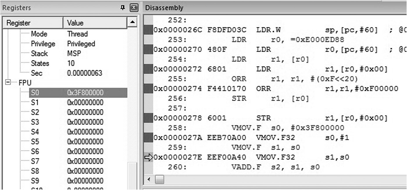
If you run the code using the Keil tools, you will see all of the registers for the processor, including the floating-point registers, in the Register window, shown in Figure 3.5. As you single-step through the code, notice that the first floating-point register, s0, eventually gets loaded with the value 0x3F800000, which is the decimal value 1.0 represented as a single-precision floating-point number. The second move operation (VMOV.F) copies that value from register s0 to s1. The VADD.F instruction adds the two numbers together, but the resulting 32-bit value, 0x40000000, definitely feels a little odd—that’s 2.0 as a single-precision floating-point value! Run the code again, replacing the value in register s0 with 0x40000000. You anticipate that the value is 4.0, but the result requires a bit of interpretation.

3.7 Program 5: Moving Values between Integer and Floating-Point Registers

It’s worth exploring one more short example. Here data is transferred between the ARM integer processor and the floating-point unit. Type in and run the following code on a Cortex-M4 microcontroller with floating-point hardware, single-stepping through each instruction to see the register values change.

	LDR 	r0,	=0xE000ED88	; Read-modify-write

	LDR 	r1,	[r0]

	ORR 	r1,	r1, #(0xF << 20)	; Enable CP10, CP11

	STR 	r1,	[r0]

	LDR	r3,	=0x3F800000	; single precision 1.0

	VMOV.F	s3,	r3	; transfer contents from ARM to FPU

	VLDR.F	s4,	=6.0221415e23	; Avogadro’s constant

	VMOV.F	r4,	s4	; transfer contents from FPU to ARM

The first four instructions are those that we saw in the previous example to enable the floating-point unit. In line five, the LDR instruction loads register r3 with the representation of 1.0 in single precision. The VMOV.F instruction then takes the value stored in an integer register and transfers it to a floating-point register, register s3. Notice that the VMOV instruction was also used earlier to transfer data between two floating-point registers. Finally, Avogadro’s constant is loaded into a floating-point register directly with the VLDR pseudo-instruction, which works just like the LDR pseudo-instruction in Programs 3 and 4. The VMOV.F instruction transfers the 32-bit value into the integer register r4. As you step through the code, watch the values move between integer and floating-point registers. Remember that the microcontroller really has little control over what these 32-bit values mean, and while there are some special values that do get treated differently in the floating-point logic, the integer logic just sees the value 0x66FF0C30 (Avogadro’s constant now converted into a 32-bit single-precision number) in register r4 and thinks nothing of it. The exotic world of IEEE-compatible floating-point numbers will be covered in great detail in Chapters 9 through 11.

3.8 Programming Guidelines

Writing assembly code is generally not difficult once you’ve become familiar with the processor’s abilities, the instructions available, and the problem you are trying to solve. When writing code for the first time, however, you should keep a few things in mind:

• Break your problem down into small pieces. Writing smaller blocks of code can often prove to be much easier than trying to tackle a large problem all at one go. The trade-off, of course, is that you must now ensure that the smaller blocks of code can share information and work together without introducing bugs in the final routine.
• Always run a test case through your finished code, even if the code looks like it will “obviously” work. Often you will find a corner case that you haven’t anticipated, and spending some time trying to break your own code is time well spent.
• Use the software tools to their fullest when writing a block of code. For example, the Keil MDK and Code Composer Studio tools provide a nice interface for setting breakpoints on instructions and watchpoints on data so that you can track the changes in registers, memory, and the condition code flags. As you step through your code, watch the changes carefully to ensure your code is doing exactly what you expect.
• Always make the assumption that someone else will be reading your code, so don’t use obscure names or labels. A frequent complaint of programmers, even experienced ones, is that they can’t understand their own code at certain points because they didn’t write down what they were thinking at the time they wrote it. Years may pass before you examine your software again, so it’s important to notate as much as possible, as carefully as possible, while you’re writing the code and it’s fresh in your mind.
• While it’s tempting to make a program look very sophisticated and clever, especially if it’s being evaluated by a teacher or supervisor, this often leads to errors. Simplicity is usually the best bet for beginning programs.
• Your first programs will probably not be optimal and efficient. This is normal. As you gain experience coding, you will learn about optimization techniques and pipeline effects later, so focus on getting the code running without errors first. Optimal code will come with practice.
• Don’t be afraid to make mistakes or try something out. The software tools that you have available make it very easy to test code sections or instructions without doing any permanent damage to anything. Write some code, run it, watch the effects on the registers and memory, and if it doesn’t work, find out why and try again!
• Using flowcharts may be useful in describing algorithms. Some programmers don’t use them, so the choice is ultimately left to the writer.
• Pay attention to initialization. When your programs or modules begin, make a note of what values you expect to find in various registers—are they to be clear? Do you need to reset certain parameters at the start of a loop? Check for constants and fixed values that can be stored in memory or in the program itself. Before using variables (register or memory contents), it’s always a good idea to set them to a known value. In some cases, this may not be necessary, e.g., if you subtracted two numbers and stored the result in a register that had not been initialized, the operation itself will set the register to a known value. However, if you use a register assuming the contents are clear, even a memory-mapped register, you can easily introduce errors in your code since some memory-mapped registers are described as undefined coming out of reset and may not be set to zero. Memory-mapped registers are examined in more detail in Chapter 16.

3.9 Exercises

1. Change Program 1, replacing the last LSL instruction with

   	ADD	r2, r1, r1, LSL #2

2. and rerun the simulation. What value is in register r2 when the code reaches the infinite loop (the B instruction)? What is the ADD instruction actually doing?
3. Using a Disassembly window, write out the seven machine codes (32-bit instructions) for Program 2.
4. How many bytes does the code for Program 2 occupy? What about Program 3?
5. Change the value in register r6 at the start of Program 2 to 12. What value is in register r7 when the code terminates? Verify that this hex number is correct.
6. Run Program 3. After the first EOR instruction, what is the value in register r0? After the second EOR instruction, what is the value in register r1?
7. Using the instructions in Program 2 as a guide, write a program for both the ARM7TDMI and the Cortex-M4 that computes 6x2 − 9x + 2 and leaves the result in register r2. You can assume x is in register r3. For the syntax of the instructions, such as addition and subtraction, see the ARM Architectural Reference Manual and the ARM v7-M Architectural Reference Manual.
8. Show two different ways to clear all the bits in register r12 to zero. You may not use any registers other than r12.
9. Using Program 3 as a guide, write a program that adds the 32-bit two’s complement representations of −149 and −4321. Place the result in register r7. Show your code and the resulting value in register r7.
10. Using Program 2 as a guide, execute the following instructions on an ARM7TDMI. Place small values in the registers beforehand. What do the instructions actually do?
    1. MOVS r6, r6, LSL #5
    2. ADD r9, r8, r8, LSL #2
    3. RSB r10, r9, r9, LSL #3
    4. (b) Followed by (c)
11. Suppose a branch instruction is located at address 0x0000FF00 in memory. What ARM instruction (32-bit binary pattern) do you think would be needed so that this B instruction could branch to itself?
12. Translate the following machine code into ARM mnemonics. What does the machine code do? What is the final value in register r2? You will want to compare these bit patterns with instructions found in the ARM Architectural Reference Manual.

    Address	Machine code
    00000000	E3A00019
    00000004	E3A01011
    00000008	E0811000
    0000000C	E1A02001

13. Using the VLDR pseudo-instruction shown in Program 5, change Program 4 so that it adds the value of pi (3.1415926) to 2.0. Verify that the answer is correct using one of the floating-point conversion tools given in the References.
14. The floating-point instruction VMUL.F works very much like a VADD.F instruction. Using Programs 4 and 5 as a guide, multiply the floating-point representation for Avogadro’s constant and 4.0 together. Verify that the result is correct using a floating-point conversion tool.