Chapter 6

Constants and Literal Pools

6.1 Introduction

One of the best things about learning assembly language is that you deal directly with hardware, and as a result, learn about computer architecture in a very direct way. It’s not absolutely necessary to know how data is transferred along busses, or how instructions make it from an instruction queue into the execution stage of a pipeline, but it is interesting to note why certain instructions are necessary in an instruction set and how certain instructions can be used in more than one way. Instructions for moving data, such as MOV, MVN, MOVW, MOVT, and LDR, will be introduced in this chapter, specifically for loading constants into a register, and while floating-point constants will be covered in Chapter 9, we’ll also see an example or two of how those values are loaded. The reason we focus so heavily on constants now is because they are a very common requirement. Examining the ARM rotation scheme here also gives us insight into fast arithmetic—a look ahead to Chapter 7. The good news is that a shortcut exists to load constants, and programmers make good use of them. However, for completeness, we will examine what the processor and the assembler are doing to generate these numbers.

6.2 The ARM Rotation Scheme

As mentioned in Chapter 1, an original design goal of early RISC processors was to have fixed-length instructions. In the case of ARM processors, the ARM and many of the Thumb-2 instructions are 32 bits long (16-bit Thumb instructions will be discussed later on). This brings us to the apparent contradiction of fitting a 32-bit constant into an instruction that is only 32 bits long. To see how this is done, let’s begin by examining the binary encoding of an ARM MOV instruction, as shown in Figure 6.1.

You can see the fields associated with the class of instruction (bits [27:25], which indicate that this is a data processing instruction), the instruction itself (bits [24:21], which would indicate a MOV instruction), and the least significant 12 bits. These last bits have quite a few options, and give the instruction great flexibility to either use registers, registers with shifts or rotates, or immediate values as operands. We will look at the case where the operand is an immediate data value, as show in Figure 6.2. Notice that the least significant byte (8 bits) can be any number between 0 and 255, and bits [11:8] of the instruction now specify a rotate value. The value is multiplied by 2, then used to rotate the 8-bit value to the right by that many bits, as shown in Figure 6.3. This means that if our bit pattern were 0xE3A004FF, for example, the machine code actually translates to the mnemonic

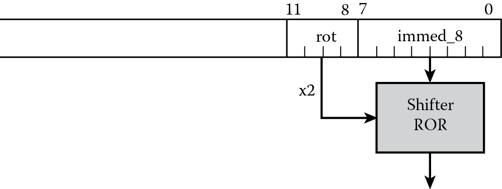
	MOV	r0, #0xFF, 8

since the least-significant 12 bits of the instruction are 0x4FF, giving us a rotation factor of 8, or 4 doubled, and a byte constant of 0xFF.

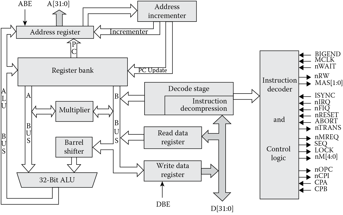
Figure 6.4 shows a simplified diagram of the ARM7 datapath logic, including the barrel shifter and main adder. While its use for logical and arithmetic shifts is covered in detail in Chapter 7, the barrel shifter is also used in the creation of constants. Barrel shifters are really little more than circuits designed specifically to shift or rotate data, and they can be built using very fast logic. ARM’s rotation scheme moves bits to the right using the inline barrel shifter, wrapping the least significant bit around to the most significant bit at the top.

With 12 bits available in an instruction and dedicated hardware for performing shifts, ARM7TDMI processors can generate classes of numbers instead of every number between 0 and 232 − 1. Analysis of typical code has shown that about half of all constants lie in the range between −15 and 15, and about ninety percent of them lie in the range between −511 and 511. You generally also need large, but simple constants, e.g., 0x4000, for masks and specifying base addresses in memory. So while not every constant is possible with this scheme, as we will see shortly, it is still possible to put any 32-bit number in a register.

Let’s examine some of the classes of numbers that can be generated using this rotation scheme. Table 6.1 shows examples of numbers you can easily generate with a MOV using an ARM7TDMI. You can, therefore, load constants directly into registers or use them in data operations using instructions such as

	MOV	r0, #0xFF			; r0 = 255

	MOV	r0, #0x1, 30			; r0 = 1020

	MOV	r0, #0x1, 26			; r0 = 4096

	ADD	r0, r2, #0xFF000000		; r0 = r2 + 0xFF000000

	SUB	r2, r3, #0x8000		; r2 = r3 − 0x8000

	RSB	r8, r9, #0x8000		; r8 = 0x8000 – r9

The Cortex-M4 can generate similar classes of numbers, using similar Thumb-2 instructions; however, the format of the MOV instruction is different, so rotational values are not specified in the same way. The second operand is more flexible, so if you wish to load a constant into a register using a MOV instruction, the constant can take the form of

• A constant that can be created by shifting an 8-bit value left by any number of bits within a word
• A constant of the form 0x00XY00XY
• A constant of the form 0xXY00XY00
• A constant of the form 0xXYXYXYXY

The Cortex-M4 can load a constant such as 0x55555555 into a register without using a literal pool, covered in the next section, which the ARM7TDMI cannot do, written as

		MOV	r3, #0x55555555

Data operations permit the use of constants, so you could use an instruction such as

		ADD r3, r4, #0xFF000000

that use the rotational scheme. If you using a MOV instruction to perform a shift operation, then the preferred method is to use ASR, LSL, LSR, ROR, or RRX instructions, which are covered in the next chapter.

Example 6.1

Calculate the rotation necessary to generate the constant 4080 using the byte rotation scheme.

Solution

Since 4080 is 1111111100002, the byte 111111112 or 0xFF can be rotated to the left by four bits. However, the rotation scheme rotates a byte to the right; therefore, a rotation factor of 28 is needed, since rotating to the left n bits is equivalent to rotating to the right by (32-n) bits. The ARM instruction would be

	MOV r0, #0xFF, 28; r0 = 4080

Example 6.2

A common method used to access peripherals on a microcontroller (ignoring bit-banding for the moment) is to specify a base address and an offset, meaning that the peripheral starts at some particular value in memory, say 0x22000000, and then the various registers belonging to that peripheral are specified as an offset to be added to the base address. The reasoning behind this scheme relies on the addressing modes available to the processor. For example, on the Tiva TM4C123GH6ZRB microcontroller, the system control base starts at address 0x400FE000. This region contains registers for configuring the main clocks, turning the PLL on and off, and enabling various other peripherals. Let’s further suppose that we’re interested in setting just one bit in a register called RCGCGPIO, which is located at an offset of 0x608 and turns on the clock to GPIO block F. This can be done with a single store instruction such as

	STR	r1, [r0, r2]

where the base address 0x400FE000 would be held in register r0, and our offset of 0x608 would be held in register r2. The most direct way to load the offset value of 0x608 into register r2 is just to say

	MOV	r2, #0x608

It turns out that this value can be created from a byte (0xC1) shifted three bits to the left, so if you were to assemble this instruction for a Cortex-M4, the 32-bit Thumb-2 instruction that is generated would be 0xF44F62C1. From Figure 6.5 below you can see that the rotational value 0xC1 occupies the lowest byte of the instruction.

The MVN (move negative) instruction, which moves a one’s complement of the operand into a register, can also be used to generate classes of numbers, such as

	MVN	r0, #0	; r0 = 0xFFFFFFFF

	MVN	r3, #0xEE	; r3 = 0xFFFFFF11

for the ARM7TDMI and Cortex-M4, and

	MVN	r0, #0xFF, 8	; r0 = 0x00FFFFFF

for the ARM7TDMI.

These rotation schemes are fine, but as a programmer, you might find this entire process a bit tiring if you have to enter dozens of constants for a data-intensive algorithm. This brings us back to our shortcut, and to numbers that cannot be built using the various methods above.

6.3 Loading Constants into Registers

We covered the topic of memory in detail in the last chapter, and we saw that there are specific instructions for loading data from memory into a register—the LDR instruction. You can create the address required by this instruction in a number of different ways, and so far we’ve examined addresses loaded directly into a register. Now the idea of an address created from the Program Counter is introduced, where register r15 (the PC) is used with a displacement value to create an address. And we’re also going to bend the LDR instruction a bit to create a pseudo-instruction that the assembler understands.

First, the shortcut: When writing assembly, you should use the following pseudo-instruction to load constants into registers, as this is by far the easiest, safest, and most maintainable way, assuming that your assembler supports it:

LDR <Rd>, =<numeric constant>

or for floating-point numbers

VLDR.F32 <Sd>, =<numeric constant>

VLDR.F64 <Dd>, =<numeric constant>

so you could say something like

	LDR		r8, =0x20000040; start of my stack

or

	VLDR.F32	s7, =3.14159165; pi

It may seem unusual to use a pseudo-instruction, but there’s a valid reason to do so. For most programmers, constants are declared at the start of sections of code, and it may be necessary to change values as code is written, modified, and maintained by other programmers. Suppose that a section of code begins as

SRAM_BASE	EQU	0x04000000

		AREA	EXAMPLE, CODE, READONLY

;

; initialization section

;

		ENTRY

		MOV	r0, #SRAM_BASE

		MOV	r1, #0xFF000000

		.

		.

		.

If the value of SRAM_BASE ever changed to a value that couldn’t be generated using the byte rotation scheme, the code will generate an error. If the code were written using

	LDR	r0, = SRAM_BASE

instead, the code will always assemble no matter what value SRAM_BASE takes. This immediately raises the question of how the assembler handles those “unusual” constants.

When the assembler sees the LDR pseudo-instruction, it will try to use either a MOV or MVN instruction to perform the given load before going further. Recall that we can generate classes of numbers, but not every number, using the rotation schemes mentioned earlier. For those numbers that cannot be created, a literal pool, or a block of constants, is created to hold them in memory, usually very near the instructions that asked for the data, along with a load instruction that fetches the constant from memory. By default, a literal pool is placed at every END directive, so a load instruction would look just beyond the last instruction in a block of code for your number. However, the addressing mode that is used to do this, called a PC-relative address, only has a range of 4 kilobytes (since the offset is only 12 bits), which means that a very large block of code can cause a problem if we don’t correct for it. In fact, even a short block of code can potentially cause problems. Suppose we have the following ARM7TDMI code in memory:

	AREA Example, CODE

	ENTRY		; mark first instruction

	BL	func1	; call first subroutine

	BL	func2	; call second subroutine

stop	B	stop	; terminate the program

func1	LDR	r0, =42	; => MOV r0, #42

	LDR	r1, =0x12345678	; => LDR r1, [PC, #N]

			; where N = offset to literal pool 1

	LDR	r2, =0xFFFFFFFF	; => MVN r2, #0

	BX	lr	; return from subroutine

	LTORG		; literal pool 1 has 0x12345678

func2	LDR	r3, =0x12345678	; => LDR r3, [PC, #N]

			; N = offset back to literal pool 1

	;LDR	r4, =0x87654321	; if this is uncommented, it fails.

			; Literal pool 2 is out of reach!

	BX	lr	; return from subroutine

BigTable

	SPACE 4200	; clears 4200 bytes of memory,

			; starting here

	END		; literal pool 2 empty

This contrived program first calls two very short subroutines via the branch and link (BL) instruction. The next instruction is merely to terminate the program, so for now we can ignore it. Notice that the first subroutine, labeled func1, loads the number 42 into register r0, which is quite easy to do with a byte rotation scheme. In fact, there is no rotation needed, since 0x2A fits within a byte. So the assembler generates a MOV instruction to load this value. The next value, 0x12345678, is too “odd” to create using a rotation scheme; therefore, the assembler is forced to generate a literal pool, which you might think would start after the 4200 bytes of space we’ve reserved at the end of the program. However, the load instruction cannot reach this far, and if we do nothing to correct for this, the assembler will generate an error. The second load instruction in the subroutine, the one setting all the bits in register r2, can be performed with a MVN instruction. The final instruction in the subroutine transfers the value from the Link Register (r14) back into the Program Counter (register r15), thereby forcing the processor to return to the instruction following the first BL instruction. Don’t worry about subroutines just yet, as there is an entire chapter covering their operation.

By inserting an LTORG directive just at the end of our first subroutine, we have forced the assembler to build its literal pool between the two subroutines in memory, as shown in Figure 6.6, which shows the memory addresses, the instructions, and the actual mnemonics generated by the assembler. You’ll also notice that the LDR instruction at address 0x10 in our example appears as

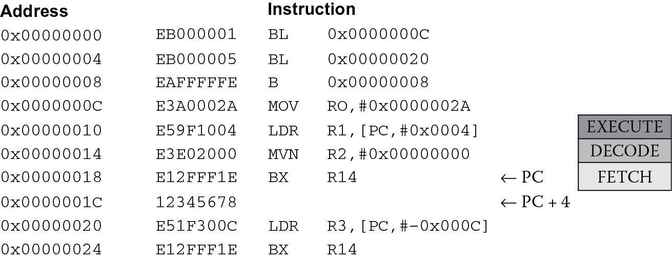
	LDR	r1, [PC,#0x0004]

which needs some explanation as well. As we saw in Chapter 5, this particular type of load instruction tells the processor to use the Program Counter (which always contains the address of the instruction being fetched from memory) modify that number (in this case add the number 8 to it) and then use this as an address. When we used the LTORG directive and told the assembler to put our literal pool between the subroutines in memory, we fixed the placement of our constants, and the assembler can then calculate how far those constants lie from the address in the Program Counter. The important thing to note in all of this is where the Program Counter is when the LDR instruction is in the pipeline’s execute stage. Again, referring to Figure 6.6, you can see that if the LDR instruction is in the execute stage of the ARM7TDMI’s pipeline, the MVN is in the decode stage, and the BX instruction is in the fetch stage. Therefore, the difference between the address 0x18 (what’s in the PC) and where we need to be to get our constant, which is 0x1C, is 4, which is the offset used to modify the PC in the LDR instruction. The good news is that you don’t ever have to calculate these offsets yourself—the assembler does that for you.

There are two more constants in the second subroutine, only one of which actually gets turned into an instruction, since we commented out the second load instruction. You will notice that in Figure 6.6, the instruction at address 0x20 is another PC-relative address, but this time the offset is negative. It turns out that the instructions can share the data already in a literal pool. Since the assembler just generated this constant for the first subroutine, and it just happens to be very near our instruction (within 4 kilobytes), you can just subtract 12 from the value of the Program Counter when the LDR instruction is in the execute stage of the pipeline. (For those readers really paying attention: the Program Counter seems to have fetched the next instruction from beyond our little program—is this a problem or not?) The second load instruction has been commented out to prevent an assembler error. As we’ve put a table of 4200 bytes just at the end of our program, the nearest literal pool is now more than 4 kilobytes away, and the assembler cannot build an instruction to reach that value in memory. To fix this, another LTORG directive would need to be added just before the table begins.

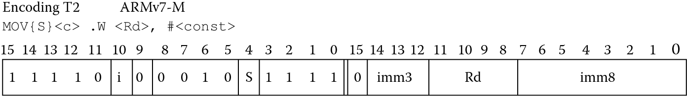
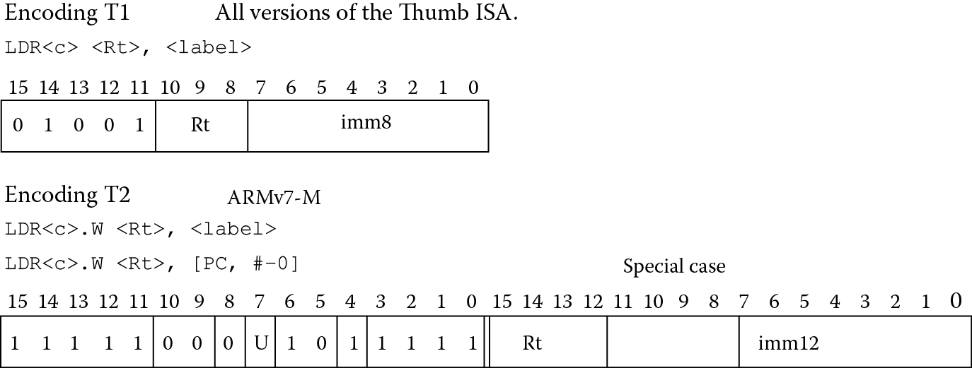
If you tried to run this same code on a Cortex-M4, you would notice several things. First, the assembler would generate code using a combination of 16-bit and 32-bit instructions, so the disassembly would look very different. More importantly, you would get an error when you tried to assemble the program, since the second subroutine, func2, tries to create the constant 0x12345678 in a second literal pool, but it would be beyond the 4 kilobyte limit due to that large table we created. It cannot initially use the value already created in the first literal pool like the ARM7TDMI did because the assembler creates the shorter (16-bit) version of the LDR instruction. Looking at Figure 6.7, you can see the offset allowed in the shorter instruction is only 8 bits, which is scaled by 4 for word accesses, and it cannot be negative. So now that the Program Counter has progressed beyond the first literal pool in memory, a PC-relative load instruction that cannot subtract values from the Program Counter to create an address will not work. In effect, we cannot see backwards. To correct this, a very simple modification of the instruction consists of adding a “.W” (for wide) extension to the LDR mnemonic, which forces the assembler to use a 32-bit Thumb-2 instruction, giving the instruction more options for creating addresses. The code below will now run without any issues.

	BL	func1	; call first subroutine

	BL	func2	; call second subroutine

stop	B	stop	; terminate the program

func1	LDR	r0, =42	; => MOV r0, #42

	LDR	r1, =0x12345678	; => LDR r1, [PC, #N]

			; where N = offset to literal pool 1

	LDR	r2, =0xFFFFFFFF	; => MVN r2, #0

	BX	lr	; return from subroutine

	LTORG		; literal pool 1 has 0x12345678

func2	LDR.W	r3, =0x12345678	; => LDR r3, [PC, #N]

			; N = offset back to literal pool 1

	;LDR	r4, =0x98765432	; if this is uncommented, it fails.

			; Literal pool 2 is out of reach!

	BX	lr	; return from subroutine

BigTable

	SPACE 4200	; clears 4200 bytes of memory,

			; starting here

So to summarize:

Use LDR <Rd > , =< numeric constant> to put a constant into an integer register.

Use VLDR <Sd > , =< numeric constant> to put a constant into a floating-point register. We’ll see this again in Section 9.9.

Literal pools are generated at the end of each section of code.

The assembler will check if the constant is available in a literal pool already, and if so, it will attempt to address the existing constant.

On the Cortex-M4, if an error is generated indicating a constant is out of range, check the width of the LDR instruction.

The assembler will attempt to place the constant in the next literal pool if it is not already available. If the next literal pool is out of range, the assembler will generate an error and you will need to fix it, probably with an LTORG or adjusting the width of the instruction used.

If you do use an LTORG, place the directive after the failed LDR pseudo-instruction and within ±4 kilobytes. You must place literal pools where the processor will not attempt to execute the data as an instruction, so put the literal pools after unconditional branch instructions or at the end of a subroutine.

6.4 Loading Constants with MOVW, MOVT

Earlier we saw that there are several ways of moving constants into registers for both the ARM7TDMI and the Cortex-M4, and depending on the type of data you have, the assembler will try and optimize the code by using the smallest instruction available, in the case of the Cortex-M4, or use the least amount of memory by avoiding literal pools, in the case of both the ARM7TDMI and the Cortex-M4. There are two more types of move instructions available on the Cortex-M4; both instructions take 16 bits of data and place them in a register. MOVW is the same operation as MOV, only the operand is restricted to a 16-bit immediate value. MOVT places a 16-bit value in the top halfword of a register, so the pair of instructions can load any 32-bit constant into a destination register, should your assembler not support the LDR pseudo-instruction, e.g., Code Composer Studio.

Example 6.3

The number 0xBEEFFACE cannot be created using a rotational scheme, nor does it fall into any of the formats, such as 0xXY00XY00, that allow a single MOV instruction to load this value into a register. You can, however, use the combination of MOVT and MOVW to create a 32-bit constant in register r3:

	MOVW		r3, #0xFACE

	MOVT		r3, #0xBEEF

6.5 Loading Addresses into Registers

At some point, you will need to load the address of a label or symbol into a register. Usually you do this to give yourself a starting point of a table, a list, or maybe a set of coefficients that are needed in a digital filter. For example, consider the ARM7TDMI code fragment below.

SRAM_BASE	EQU	0x04000000

	AREA	FILTER, CODE

dest	RN0	; destination pointer

image	RN1	; image data pointer

coeff	RN2	; coefficient table pointer

pointer	RN3	; temporary pointer

	ENTRY

	CODE32

Main

	; initialization area

	LDR	dest, =#SRAM_BASE	; move memory base into dest

	MOV	pointer, dest	; current pointer is destination

	ADR	image, image_data	; load image data pointer

	ADR	coeff, cosines	; load coefficient pointer

	BL	filter	; execute one pass of filter

	.

	.

	.

	ALIGN

image_data

	DCW	0x0001,0x0002,0x0003,0x0004

	DCW	0x0005,0x0006,0x0007,0x0008

	.

	.

	.

cosines

	DCW	0x3ec5,0x3537,0x238e,0x0c7c

	DCW	0xf384,0xdc72,0xcac9,0xc13b

	.

	.

	.

	END

While the majority of the program is still to be written, you can see that if we were to set up an algorithm, say an FIR filter, where you had some data stored in memory and some coefficients stored in memory, you would want to set pointers to the start of each set. This way, a register would hold a starting address. To access a particular data value, you would simply use that register with an offset of some kind.

We have seen the directives EQU and RN already in Chapter 4, but now we actually start using them. The first line equates the label SRAM_BASE to a number, so that when we use it in the code, we don’t have to keep typing that long address, similar to the #DEFINE statement in C. The RN directives give names to our registers r0, r1, r2, and r3, so that we can refer to them by their function rather than by their number. You don’t have to do this, but often it’s helpful to know a register’s use while programming. The first two instructions load a known address (called an absolute address, since it doesn’t move if you relocate your code in memory) into registers r0 and r3. The third and fourth instructions are the pseudo-instruction ADR, which is particularly useful at loading addresses into a register. Why do it this way? Suppose that this section of code was to be used along with other blocks. You wouldn’t necessarily know exactly where your data starts once the two sections are assembled, so it’s easier to let the assembler calculate the addresses for you. As an example, if image_data actually started at address 0x8000 in memory, then this address gets moved into register r1, which we’ve renamed. However, if we change the code, move the image data, or add another block of code that we write later, then this address will change. By using ADR, we don’t have to worry about the address.

Example 6.4

Let’s examine another example, this time to see how the ADR pseudo-instruction actually gets converted into real ARM instructions. Again, the code in this example doesn’t actually do anything except set up pointers, but it will serve to illustrate how ADR behaves.

		AREA	adrlabel,CODE,READONLY

		ENTRY		; mark first instruction to execute

Start	BL	func	; branch to subroutine

stop	B	stop	; terminate

		LTORG		; create a literal pool

func	ADR	r0, Start	; => SUB r0, PC, #offset to Start

		ADR	r1, DataArea	; =>  ADD r1, PC, #offset to DataArea

		;ADR	r2, DataArea + 4300	; This would fail because the offset

				; cannot be expressed by operand2 of ADD

		ADRL	r2, DataArea + 4300	; => ADD r2, PC, #offset1

				; ADD	r2, r2, #offset2

		BX	lr	; return

DataArea

		SPACE	8000	; starting at the current location,

				; clears an 8000-byte area of memory to 0

		END

You will note that the program calls a subroutine called func, using a branch and link operation (BL). The next instruction is for ending the program, so we really only need to examine what happens after the LTORG directive. The subroutine begins with a label, func, and an ADR pseudo-instruction to load the starting address of our main program into register r0. The assembler actually creates either an ADD or SUB instruction with the Program Counter to do this. Similar to the LDR pseudo-instruction we saw previously, by knowing the value of the Program Counter at the time when this ADD or SUB reaches the execute stage of the pipeline, we can simply take that value and modify it to generate an address. The catch is that the offset must be a particular type of number. For ARM instructions, that number must be one that can be created using a byte value rotated by an even number of bits, exactly as we saw in Section 6.2 (if rejected by the assembler, it will generate an error message to indicate that an offset cannot be represented by 0–255 and a rotation). For 32-bit Thumb instructions, that number must be within ±4095 bytes of a byte, half-word, or word-aligned address. If you notice the second ADR in this example, the distance between the instruction and the label DataArea is small enough that the assembler will use a simple ADD instruction to create the constant.

The third ADR tries to create an address where the label is on the other side of an 8000-byte block of memory. This doesn’t work, but there is another pseudo-instruction: ADRL. Using two operations instead of one, the ADRL will calculate an offset that is within a range based on the addition of two values now, both created by the byte rotation scheme mentioned above (for ARM instructions). There is a fixed range for 32-bit Thumb instructions of ±1MB. You should note that if you invoke an ADRL pseudo-instruction in your code, it will generate two operations even if it could be done using only one, so be careful in loops that are sensitive to cycle counts. One other important point worth mentioning is that the label used with ADR or ADRL must be within the same code section. If a label is out of range in the same section, the assembler faults the reference. As an aside, if a label is out of range in other code sections, the linker faults the reference.

There is yet another way of loading addresses into registers, and it is exactly the same as the LDR pseudo-instruction we saw earlier for loading constants. The syntax is

LDR <Rd>, =label

In this instance, the assembler will convert the pseudo-instruction into a load instruction, where the load reads the address from a literal pool that it creates. As with the case of loading constants, you must ensure that a literal pool is within range of the instruction. This pseudo-instruction differs from ADR and ADRL in that labels outside of a section can be referenced, and the linker will resolve the reference at link time.

Example 6.5

The example below shows a few of the ways the LDR pseudo-instruction can be used, including using labels with their own offsets.

	AREA	LDRlabel, CODE, READONLY

	ENTRY		; Mark first instruction to execute

start

	BL	func1	; branch to first subroutine

	BL	func2	; branch to second subroutine

stop	B	stop	; terminate

func1

	LDR	r0, =start	;=> LDR R0, [PC, #offset into Literal Pool 1]

	LDR	r1, =Darea + 12	;=> LDR R1, [PC, #offset into Lit. Pool 1]

	LDR	r2, =Darea + 6000	;=> LDR R2, [PC, #offset into Lit. Pool 1]

	BX	lr	; return

	LTORG

func2

	LDR	r3, =Darea + 6000	; => LDR R3, [PC, #offset into Lit. Pool 1]

			; (sharing with previous literal)

	; LDR	r4, =Darea + 6004	; if uncommented produces an error

			; as literal pool 2 is out of range

	BX	lr	; return

Darea

	SPACE	8000	; starting at the current location, clears

			; an 8000-byte area of memory to zero

	END		; literal pool 2 is out of range of the LDR

			; instructions above

You can see the first three LDR statements in the subroutine func1 would actually be PC-relative loads from a literal pool that would exist in memory at the LTORG statement. Additionally, the first load statement in the second subroutine could use the same literal pool to create a PC-relative offset. As the SPACE directive has cleared an 8000-byte block of memory, the second load instruction cannot reach the second literal pool, since it must be within 4 kilobytes.

So to summarize:

Use the pseudo-instruction

ADR <Rd>, label

to put an address into a register whenever possible. The address is created by adding or subtracting an offset to/from the PC, where the offset is calculated by the assembler.

If the above case fails, use the ADRL pseudo-instruction, which will calculate an offset using two separate ADD or SUB operations. Note that if you invoke an ADRL pseudo-instruction in your code, it will generate two operations even if it could be done using only one.

Use the pseudo-instruction

LDR <Rd>, =label

if you plan to reference labels in other sections of code, or you know that a literal table will exist and you don’t mind the extra cycles used to fetch the literal from memory. Use the same caution with literal pools that you would for the construct

LDR <Rd>, =constant

Consult the Assembler User’s Guide (ARM 2008a) for more details on the use of ADR, ADRL and LDR for loading addresses.

6.6 Exercises

1. What constant would be loaded into register r7 by the following instructions?
   1. MOV r7, #0x8C, 4
   2. MOV r7, #0x42, 30
   3. MVN r7, #2
   4. MVN r7, #0x8C, 4
2. Using the byte rotation scheme described for the ARM7TDMI, calculate the instruction and rotation needed to load the following constants into register r2:
   1. 0xA400
   2. 0x7D8
   3. 0x17400
   4. 0x1980
3. Tell whether or not the following constants can be loaded into an ARM7TDMI register without creating a literal pool and using only a single instruction:
   1. 0x12340000
   2. 0x77777777
   3. 0xFFFFFFFF
   4. 0xFFFFFFFE
4. Tell whether or not the following constants can be loaded into a Cortex-M4 register without creating a literal pool and using only a single instruction:
   1. 0xEE00EE00
   2. 0x09A00000
   3. 0x33333373
   4. 0xFFFFFFFE
5. What is the best way to put a numeric constant into a register, assuming your assembler supports the method?
6. Where is the best place to put literal pool data?
7. Suppose you had the following code:

   		AREA SAMPLE, CODE,READONLY

   		ENTRY

   	start

   		MOV	r12, #SRAM_BASE

   		ADD	r0, r1, r2

   		MOV	r0, #0x18

   		BL	routine1

   		.

   		.

   		.

   	routine1

   		STM	sp!, {r0-r3,lr}

   		.

   		.

   		.

   		END

8. Describe two ways to load the label routine1 into register r3, noting any restrictions that apply.
9. Describe the difference between ADR and ADRL.
10. Give the instruction(s) to perform the following operations for both the ARM7TDMI and the Cortex-M4:
    1. Add 0xEC00 to register r6, placing the sum in register r4.
    2. Subtract 0xFF000000 from register r12, placing the result in register r7.
    3. Add the value 0x123456AB to register r7, placing the sum in register r12.
    4. Place a two’s complement representation of −1 into register r3.
11. Suppose you had the following code and you are using the Keil tools:

    		.

    		.

    		.

    		BL func1	; call first subroutine

    		BL func2	; call second subroutine

    	stop	B stop	; terminate the program

    	func1	MOV r2, #0

    		LDR r1, =0xBABEFACE

    		LDR r2, =0xFFFFFFFC

    		MOV pc, lr	; return from subroutine

    		LTORG	; literal pool 1 has 0xBABEFACE

    	func2	LDR r3, =0xBABEFACE

    		LDR r4, =0x66666666

    		MOV pc, lr	; return from subroutine

    	BigTable

    		SPACE 3700	; clears 3700 bytes of memory,

    			; starting here

    		.

    		.

    		.

12. On an ARM7TDMI, will loading 0x66666666 into register r4 cause an error? Why or why not? What about on a Cortex-M4?
13. The ARM branch instruction—B—provides a ±32 MB branching range. If the Program Counter is currently 0x8000 and you need to jump to address 0xFF000000, how do you think you might do this?
14. Assuming that the floating-point hardware is already enabled (CP10 and CP11), write the instructions to load the floating-point register s3 with a quiet NaN, or 0x7FC00000. (Hint: use Program 5 from Chapter 3 as a guide.) You can write it using either the Keil tools or the CCS tools.