Table of Contents for

The Rootkit Arsenal: Escape and Evasion in the Dark Corners of the System, 2nd Edition

Chapter 8    Defeating Executable Analysis

---

 

With regard to disk analysis, data hiding and data transformation can only go so far. At the end of the day, there will have to be at least one executable that initiates everything (e.g., extracts and decrypts the core payload), and this executable cannot be hidden or encrypted. It must stand out in the open, in the crosshairs of the forensic investigator as an unknown executable.

Once the forensic investigator has found the subset of executable binaries in his or her group of suspicious files, he or she will start performing executable file analysis. There are two variations of executable analysis that can be performed:

  Static executable analysis (think composition).

  Runtime executable analysis (think behavior).

Static analysis looks at the executable, its composition and its surroundings, without actually launching it. This phase of inspection essentially focuses on the suspect file as an inert series of bytes, gleaning whatever is possible from a vantage point that’s relatively secure.

Runtime analysis aims to learn about the operation of an executable by monitoring it during execution in the confines of a controlled environment. In this case, the emphasis is on behavior rather than mere static composition.

8.1    Static Analysis

---

Static analysis is the less risky cousin of runtime analysis. We take out our scalpel and other surgical tools and try to dissect the unknown executable as an inanimate binary. In the end, the nature of static analysis is also what makes it easier to undermine. Thus, static analysis often transitively leads to runtime analysis as the investigator seeks to get a deeper understanding of an application’s composition and behavior.

Scan for Related Artifacts

Having isolated a potential rootkit, the forensic investigator might hunt through the registry for values that include the binary’s file name. For instance, if the executable is registered as a KMD, it’s bound to pop up under the following key:

HKLM\SYSTEM\CurrentControlSet\Services

This sort of search can be initiated at the command line.

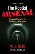
If nothing exists in the registry, the executable may store its configuration parameters in a text file. These files, if they’re not encrypted, can be a treasure trove of useful information as far as determining what the executable does. Consider the following text file snippet:

There may be members of the reading audience who recognize this as part of the .ini file for Hacker Defender.

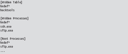
Verify Digital Signatures

If an unknown executable is trying to masquerade as a legitimate system file, you can try to flush it out by checking its digital signature. To this end, the sigcheck.exe utility in the Sysinternals tool suite proves useful.

Just be aware, as described earlier in the book (e.g., the case of the Stuxnet rootkit), that digital signatures do not always provide bulletproof security. If you’re suspicious of a particular system binary, do a raw binary comparison against a known good copy.

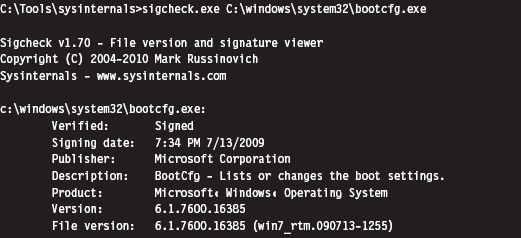
You can also use the SFC.exe (System File Checker) tool to verify the integrity of protected system files. As described in Knowledge Base (KB) Article 929833, checking a potentially corrupted system binary is pretty straightforward.

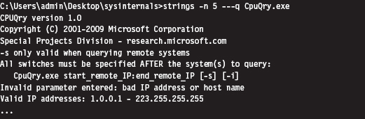
Dump String Data

Another quick preliminary check that a forensic investigator can do is to search an unknown executable for strings. If you can’t locate a configuration file, sometimes its path and command-line usage will be hard-coded in the executable. This information can be enlightening.

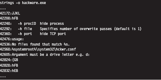
The previous command uses the strings.exe tool from Sysinternals. The -o option causes the tools to print out the offset in the file where each string was located. If you prefer a GUI, Foundstone has developed a string extractor called BinText.¹

Inspect File Headers

One way in which a binary gives away its purpose is in terms of the routines that it imports and exports. For example, a binary that imports the Ws2_32.dll probably implements network communication of some sort because it’s using routines from the Windows Sockets 2 API. Likewise, a binary that imports ssleay32.dll (from the OpenSSL distribution) is encrypting the packets that it sends over the network and is probably trying to hide something.

The dumpbin.exe tool that ships with the Windows SDK can be used to determine what an executable imports and exports. From the standpoint of static analysis, dumpbin.exe is also useful because it indicates what sort of binary we’re working with (i.e., EXE, DLL, SYS, etc.), whether symbol information has been stripped, and it can display the binary composition of the file.

Dumpbin.exe recovers this information by trolling through the file headers of a binary. Headers are essentially metadata structures embedded within an executable. On Windows, the sort of metadata that you’ll encounter is defined by the Microsoft Portable Executable (PE) file format specification.² To get the full Monty, use the /all option when you invoke dumpbin.exe. Here’s an example of the output that you’ll see (I’ve truncated things a bit to make it more readable and highlighted salient information):

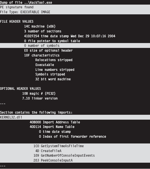
If you prefer a GUI, Wayne Radburn has developed a tool called PEView.exe that offers equivalent information in a tree-view format.³

Disassembly and Decompilation

At the end of the day, the ultimate authority on what a binary does and does not do is its machine instruction encoding. Thus, another way to gain insight into the nature of an executable (from the standpoint of static analysis) is to take a look under the hood.

Although this might seem like the definitive way to see what’s happening, it’s more of a last resort than anything else because reversing a moderately complicated piece of software can be extremely resource-intensive. It’s very easy for the uninitiated to get lost among the trees, so to speak. Mind you, I’m not saying that reversing is a bad idea or won’t yield results. I’m observing the fact that most forensic investigators, faced with a backlog of machines to process, will typically only target the machine code after they’ve tried everything else.

The process of reversing an executable can be broken down into two phases: disassembly and decompilation (see Figure 8.1).

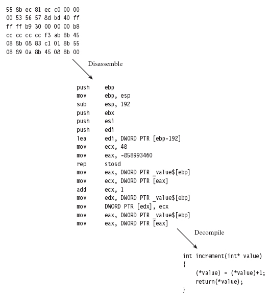
Figure 8.1

The process of disassembly takes the raw machine code and translates it into a slightly more readable set of mnemonics know as assembly code. There are different ways in which this can be done:

  Linear sweep disassembly.

  Recursive traversal disassembly.

Linear sweep disassembly plows through machine code head on, sequentially translating one machine instruction after another. This can lead to problems in the event of embedded data or intentionally injected junk bytes.

Recursive traversal disassembly tries to address these problems by sequentially translating machine code until a control transfer instruction is encountered. At this point, the disassemble attempts to identify potential destinations of the control transfer instruction and then recursively continues to disassemble the code at those destinations. This is all nice and well, until a jump is encountered where the destination is determined at runtime.

The tool of choice for most reversers on Windows is OllyDbg.⁴ It’s a free user-mode debugger that uses a smart, tricked-out implementation of the recursive traversal technique. Another free option is simply to stick with the debuggers that ship with the WDK, which sport extensions that can come in handy when dealing with code that relies heavily on obscure Windows features.

If you have a budget, you might want to consider investing in the IDA Pro disassembler from Hex-Rays.⁵ To get a feel for the tool, the folks at Hex-Rays offer a limited freeware version. Yet another commercial tool is PE Explorer from Heaventools.⁶

Decompilation takes things to the next level by reconstructing higher-level constructs from an assembly code (or platform-neutral intermediate code) representation. Suffice it to say that the original intent of the developer and other high-level artifacts are often lost in the initial translation to machine code, making decompilation problematic.

Some people have likened this process to unscrambling an egg. Suffice it to say that the pool of available tools in this domain is small. Given the amount of effort involved in developing a solid decompiler, your best bet is probably to go with the IDA Pro decompiler plug-in sold by Hex-Rays.

8.2    Subverting Static Analysis

---

In the past, electronic parts on a printed circuit board were sometimes potted in an effort to make them more difficult to reverse engineer. This involved encapsulating the components in a thermosetting resin that could be cured in such a way that it could not be melted later on. The IBM 4758 cryptoprocessor is a well-known example of a module that’s protected by potting. In this section, we’ll look at similar ways to bundle executable files in a manner that discourages reversing.

Data Transformation: Armoring

Armoring is a process that aims to hinder the analysis through the anti-forensic strategy of data transformation. In other words, we take the bytes that make up an executable and we alter them to make them more difficult to understand. Armoring is a general term that encompasses several related, and possibly overlapping, tactics (obfuscation, encryption, etc.).

The Underwriters Laboratory (UL)⁷ has been rating safes and vaults for more than 80 years. The highest safe rating, TXTL60, is given to products that can fend off a well-equipped safe cracker for at least 60 minutes (even if he is armed with 8 ounces of nitroglycerin). What this goes to show is that there’s no such thing as a burglar-proof safe. Given enough time and the right tools, any safe can be compromised.

Likewise, there are limits to the effectiveness of armoring. With sufficient effort, any armored binary can be dissected and laid bare. Having issued this disclaimer, our goal is to raise the complexity threshold just high enough so that the forensic investigator decides to call it quits. This goes back to what I said earlier in the chapter; anti-forensics is all about buying time.

Armoring: Cryptors

A cryptor is a program that takes an ordinary executable and encrypts it so that its contents can’t be examined. During the process of encrypting the original executable, the cryptor appends a minimal stub program (see Figure 8.2). When the executable is invoked, the stub program launches and decrypts the encrypted payload so that the original program can run.

Implementing a cryptor isn’t necessarily difficult, it’s just tedious. Much of it depends upon understanding the Windows PE file format (both in memory and on disk). The process depicted in Figure 8.2 tacitly assumes that we’re encapsulating an entire third-party binary that we didn’t create ourselves.

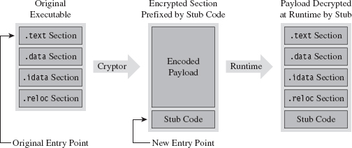
Figure 8.2

In this case, the binary and all of its sections must be wrapped up into a single Windows PE file section. This will require our stub program to assume some of the duties normally relegated to the Windows loader. When we reach the chapter on memory-resident code, we’ll see what type of responsibilities this entails.

Assuming we have access to the source code of the original program, things change slightly (see Figure 8.3). In this case, we’ll need to modify the makeup of the program by adding two new sections. The sections are added using special pre-processor directives. The first new section (the .code section) will be used to store the applications code and data. The existing code and data sections will be merged into the new .code section using the linker’s /MERGE option. The second new section (the .stub section) will implement the code that decrypts the rest of the program at runtime and re-routes the path of execution back to the original entry point.

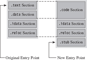
Figure 8.3

Once we’ve re-compiled the source code, the executable (with its .code and .stub sections) will be in a form that the cryptor can digest. The cryptor will map the executable file into memory and traverse its file structure, starting with the DOS header, then the Windows PE header, then the PE optional header, and then finally the PE section headers. This traversal is performed so that we can find the location of the .code section, both on disk and in memory. The location of the .code section in the file (its size and byte offset) is used by the cryptor to encrypt the code and data while the executable lays dormant. The location of the .code section in memory (its size and base address) is used to patch the stub so that it decrypts the correct region of memory at runtime.

The average executable can be composed of several different sections (see Table 8.1). You can examine the metadata associated with them using the dumpbin.exe command with the /HEADERS option.

Table 8.1 PE Sections

Section Name	Description
.text	Executable machine code instructions
.data	Global and static variable storage (initialized at compile time)
.bss	Global and static variable storage (NOT initialized at compile time)
.textbss	Enabled incremental linking
.rsrc	Stores auxiliary binary objects
.idata	Stores information on imported library routines
.edata	Stores information on exported library routines
.reloc	Allows the executable to be loaded at an arbitrary address
.rdata	Mostly random stuff

The .text section is the default section for machine instructions. Typically, the linker will merge all of the .text sections from each .OBJ file into one great big unified .text section in the final executable.

The .data section is the default section for global and static variables that are initialized at compile time. Global and static variables that aren’t initialized at compile time end up in the .bss section.

The .textbss section facilitates incremental linking. In the old days, linking was a batch process that merged all of the object modules of a software project into a single executable by resolving symbolic cross-references. The problem with this approach is that it wasted time because program changes usually only involved a limited subset of object modules. To speed things up, an incremental linker processes only modules that have recently been changed. The Microsoft linker runs in incremental mode by default. You can remove this section by disabling incremental linking with the /INCREMENTAL:NO linker option.

The .rsrc section is used to store module resources, which are binary objects that can be embedded in an executable. For example, custom-built mouse cursors, fonts, program icons, string tables, and version information are all standard resources. A resource can also be some chunk of arbitrary data that’s needed by an application (e.g., like another executable).

The .idata section stores information needed by an application to import routines from other modules. The import address table (IAT) resides in this section. Likewise, the .edata section contains information about the routines that an executable exports.

The .reloc section contains a table of base relocation records. A base relocation is a change that needs to be made to a machine instruction, or literal value, in the event that the Windows loader wasn’t able to load a module at its preferred base address. For example, by default the base address of .EXE files is 0×400000. The default base address of .DLL modules is 0×10000000. If the loader can’t place a module at its preferred base address, the module will need its relocation records to resolve memory addresses properly at runtime. You can preclude the .reloc section by specifying the /FIXED linker option. However, this will require the resulting executable to always be loaded at its preferred base address.

The .rdata section is sort of a mixed bag. It stores debugging information in .EXE files that have been built with debugging options enabled. It also stores the descriptive string value specified by the DESCRIPTION statement in an application’s module-definition (.DEF) file. The DEF file is one way to provide the linker with metadata related to exported routines, file section attributes, and the like. It’s used with DLLs mostly.

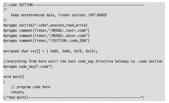
Let’s look at some source code to see exactly how this cryptor works. We’ll start by observing the alterations that will need to be made to prepare the target application for encryption. Specifically, the first thing that needs to be done is to declare the new .code section using the #pragma section directive.

Then we’ll issue several #pragma comment directives with the /MERGE option so that the linker knows to merge the .data section and .text section into the .code section. This way all of our code and data is in one place, and this makes life easier for the cryptor. The cryptor will simply read the executable looking for a section named .code, and that’s what it will encrypt.

The last of the #pragma comment directives (of this initial set of directives) uses the /SECTION linker option to adjust the attributes of the .code section so that it’s executable, readable, and writeable. This is a good idea because the stub code will need to write to the .code section in order to decrypt it.

You can verify that the .text and .data section are indeed merged by examining the compiled executable with a hex editor. The location of the .code section is indicated by the “file pointer to raw data” and “size of raw data” fields output by the dumpbin.exe command using the /HEADERS option.

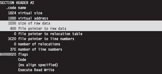
If you look at the bytes that make up the code section, you’ll see the hex digits 0×CAFEBABE. This confirms that both data and code have been fused together into the same region.

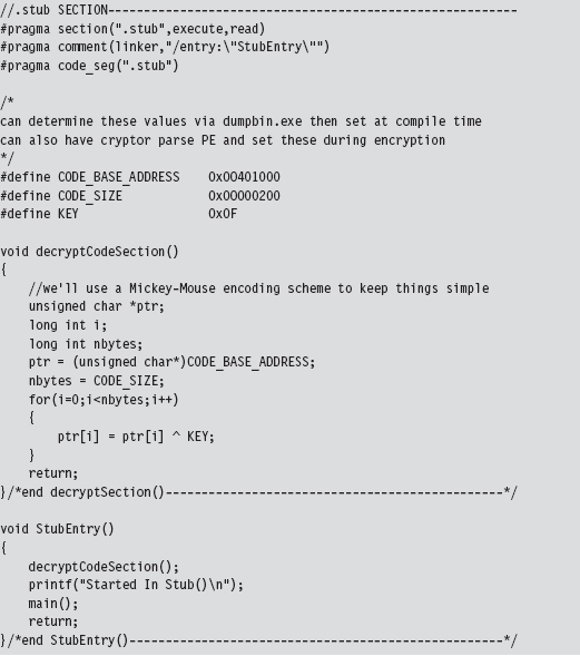
Creating the stub is fairly simple. You use the #pragma section directive to announce the existence of the .stub section. This is followed by a #pragma comment directive that uses the /ENTRY linker option to re-route the program’s entry point to the StubEntry() routine. This way, when the executable starts up, it doesn’t try to execute main(), which will consist of encrypted code!

For the sake of focusing on the pure mechanics of the stub, I’ve stuck to brain-dead XOR encryption. You can replace the body of the decryptCodeSection() routine with whatever.

Also, the base address and size of the .code section were determined via dumpbin.exe. This means that building the stub correctly may require the target to be compiled twice (once to determine the .code section’s parameters, and a second time to set the decryption parameters). An improvement would be to automate this by having the cryptor patch the stub binary and insert the proper values after it encrypts the .code section.

As mentioned earlier, this approach assumes that you have access to the source code of the program to be encrypted. If not, you’ll need to embed the entire target executable into the stub program somehow, perhaps as a binary resource or as a byte array in a dedicated file section. Then the stub code will have to take over many of the responsibilities assumed by the Windows loader:

  Mapping the encrypted executable file into memory.

  Resolving import addresses.

  Apply relocation record fix-ups (if needed).

Depending on the sort of executable you’re dealing with, this can end up being a lot of work. Applications that use more involved development technologies like COM or COM+ can be particularly sensitive.

Another thing to keep in mind is that the IAT of the target application in the .idata section is not encrypted in this example, and this might cause some information leakage. It’s like telling the police what you’ve got stashed in the trunk of your car. One way to work around this is to rely on runtime dynamic-linking, which doesn’t require the IAT. Or, you can go to the opposite extreme and flood the IAT with entries so that the routines that you do actually use can hide in the crowd, so to speak.

Now let’s look at the cryptor itself. It starts with a call to getHMODULE(), which maps the target executable into memory. Then it walks through the executable’s header structures via a call to the GetCodeLoc() routine. Once the cryptor has recovered the information that it needs from the headers, it encrypts the .code section of the executable.

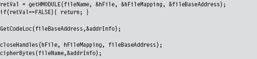
The really important bits of information that we extract from the target executable’s headers are deposited in an ADDRESS_INFO structure. In order to decrypt and encrypt the .code section, we need to know both where it resides in memory (at runtime) and in the .EXE file on disk.

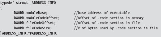
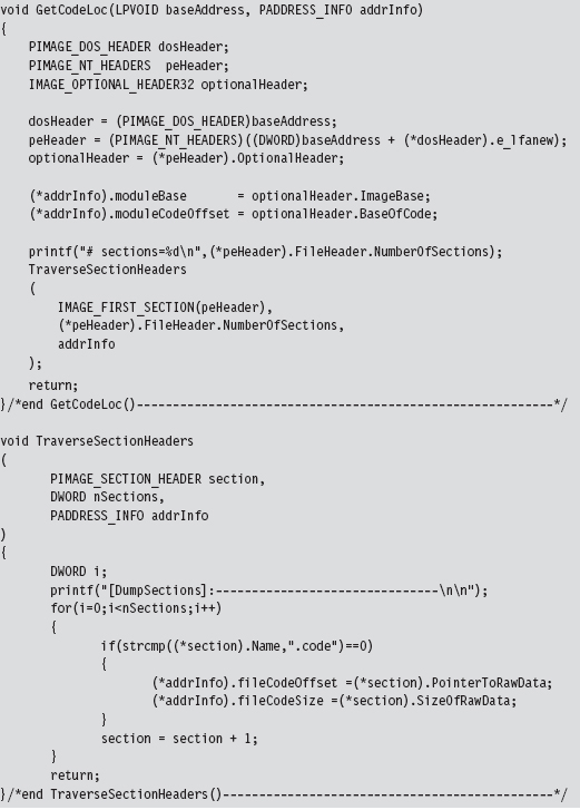
Looking at the body of the GetCodeLoc() routine (and the subroutine that it invokes), we can see that the relevant information is stored in the IMAGE_OPTIONAL_HEADER and in the section header table that follows the optional header.

Once the ADDRESS_INFO structure has been populated, processing the target executable is as simple as opening the file up to the specified offset and encrypting the necessary number of bytes.

This isn’t the only way to design a cryptor. There are various approaches that involve varying degrees of complexity. What I’ve given you is the software equivalent of an economy-class rental car. If you’d like to examine the source code of a more fully featured cryptor, you can check out Yoda’s Cryptor online.⁸

Key Management

One of the long-standing problems associated with using an encrypted executable is that you need to find somewhere to stash the encryption key. If you embed the key within the executable itself, the key will, no doubt, eventually be found. Though, as mentioned earlier in the chapter, if you’re devious enough in terms of how well you camouflage the key, you may be able to keep the analyst at bay long enough to foil static analysis.

One way to buy time involves encrypting different parts of the executable with different keys, where the keys are generated at runtime by the decryptor stub using a tortuous key generation algorithm. Although the forensic investigator might be able to find individual keys in isolation, the goal is to use so many that the forensic investigator will have a difficult time getting all of them simultaneously to acquire a clear, unencrypted view of the executable.

Another alternative is to hide the key somewhere—outside of the encrypted executable—that the forensic investigator might not look, like an empty disk sector reserved for the MFT (according to The Grugq, “reserved” disk storage usually means “reserved for attackers”). If you don’t want to take the chance of storing the key on disk, and if the situation warrants it, you could invest the effort necessary to hide the key in PCI-ROM.

Yet another alternative is use a key that depends upon the unique environmental factors of the host machine that the executable resides on. This sort of key is known as an environmental key, and the idea was proposed publicly in a paper by Riordan and Schneier.⁹ The BRADLEY virus, presented by Major Eric Filiol in 2005, uses environmental key generation to support code armoring.¹⁰

Armoring: Packers

A packer is like a cryptor, only instead of encrypting the target binary, the packer compresses it. Packers were originally used to implement self-extracting applications, back when disk storage was at a premium and a gigabyte of drive space was unthinkable for the typical user. For our purposes, the intent of a packer is the same as that for a cryptor: We want to be able to hinder disassembly. Compression provides us with a way to obfuscate the contents of our executable.

One fundamental difference between packers and cryptors is that packers don’t require an encryption key. This makes packers inherently less secure. Once the compression algorithm being used has been identified, it’s a simple matter to reverse the process and extract the binary for analysis. With encryption, you can know exactly which algorithm is in use (e.g., 3DES, AES, GOST) and still not be able to recover the original executable.

One of the most prolific executable packers is UPX (the Ultimate Packer for eXecutables).¹¹ Not only does it handle dozens of different executable formats, but also its source code is available online. Needless to say that the source code to UPX is not a quick read. If you’d like to get your feet wet before diving into the blueprints of the packer itself, the source code to the stub program that does the decompression can be found in the src/stub directory of the UPX source tree.

In terms of its general operation, the UPX packer takes an executable and consolidates its sections (.text, .data, .idata, etc.) into a single section named UPX1. By the way, the UPX1 section also contains the decompression stub program that will unpack the original executable at runtime. You can examine the resulting compressed executable with dumpbin.exe to confirm that it consists of three sections:

  UPX0

  UPX1

  .rsrc

At runtime (see Figure 8.4), the UPX0 section is loaded into memory first, at a lower address. The UPX0 section is literally just empty space. On disk, UPX0 doesn’t take up any space at all. Its raw data size in the compressed executable is zero, such that both UPX0 and UPX1 start at the same file offset in the compressed binary. The UPX1 section is loaded into memory above UPX0, which makes sense because the stub program in UPX1 will decompress the packed executable starting at the beginning of UPX0. As decompression continues, eventually the unpacked data will grow upwards in memory and overwrite data in UPX1.

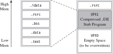
Figure 8.4

The UPX stub wrapper is a minimal program, with very few imports. You can verify this using the ever-handy dumpbin.exe tool.

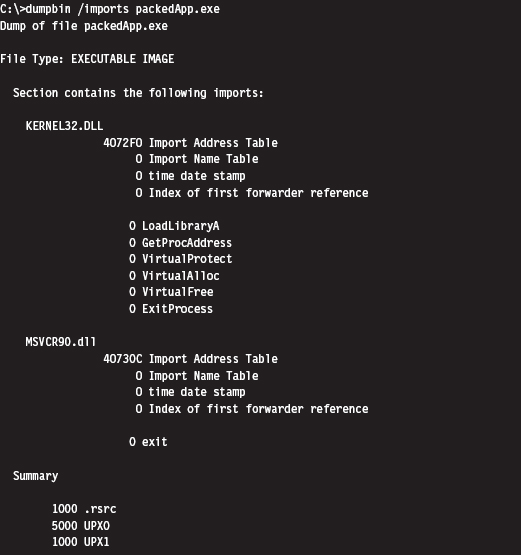
The problem with this import signature is that it’s a dead giveaway. Any forensic investigator who runs into a binary that has almost no embedded string data, very few imports, and sections named UPX0 and UPX1 will immediately know what’s going on. Unpacking the compressed executable is then just a simple matter of invoking UPX with the –d switch.

Armoring: Metamorphic Code

The concept of metamorphic code was born out of a desire to evade the signature recognition heuristics implemented by anti-virus software. The basic idea is to take the machine code that constitutes the payload of a virus and rewrite it using different, but equivalent, machine code. In other words, the code should do the same thing using a different sequence of instructions.

Recall the examples I gave earlier in the book where I demonstrated how there were several distinct, but equivalent, ways to implement a transfer of program control (e.g., with a JMP instruction, or a CALL, or a RET, etc.).

In volume 6 of the online publication 29A, a malware developer known as the Mental Driller presents a sample implementation of a metamorphic engine called MetaPHOR.¹² The structure of this engine is depicted in Figure 8.5. As you can see, because of the complexity of the task that the engine must accomplish, it tends to be much larger than the actual payload that it processes.

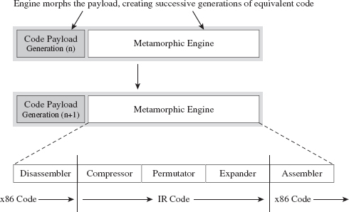
Figure 8.5

The fun begins with the disassembler, which takes the platform-specific machine code and disassembles it into a platform-neutral intermediate representation (IR), which is easier to deal with from an engineering standpoint. The compressor takes the IR code and removes unnecessary code that was added during an earlier pass through the metamorphic engine. This way, the executable doesn’t grow uncontrollably as it mutates.

The permutation component of the engine is what does most of the transformation. It takes the IR code and rewrites it so that it implements the same algorithm using a different series of instructions. Then, the expander takes this output and randomly sprinkles in additional code further to obfuscate what the code is doing. Finally, the assembler takes the IR code and translates it back into the target platform’s machine code. The assembler also performs all the tedious address and relocation fix-ups that are inevitably necessary as a result of the previous stages.

The random nature of permutation and compression/expansion help to ensure that successive generations bear no resemblance to their parents. However, this can also make debugging the metamorphic engine difficult. As time passes, it changes shape, and this can introduce instance-specific bugs that somehow must be traced back to the original implementation. As Stan Lee proclaimed in his comic books, with great power comes great responsibility. God bless you Stan.

But wait a minute! How does this help us? Assuming that this is a targeted attack using a custom rootkit, we’re not really worried about signature recognition. Are we? We’re more concerned with making it difficult to perform a static analysis of our rootkit.

It’s possible to draw on the example provided by metamorphic malware and extrapolate it a step further. Specifically, we started with an embedded metamorphic engine that translates x86 machine code into IR bytecode and then back into x86 machine code. Why even bother with x86 to IR translation? Why not just replace the machine code payload with platform-neutral bytecode and deploy an embedded virtual machine that executes the bytecode at runtime? In other words, our rootkit logic is implemented as an arbitrary bytecode, and it has its own built-in virtual machine to interpret and execute the bytecode (see Figure 8.6). This is an approach that’s so effective that it has been adopted by commercial software protection tools.¹³

Figure 8.6

One way to augment this approach would be to encode our rootkit’s application logic using more than one bytecode instruction set. There are a number of ways this could be implemented. For example, you could implement a common runtime environment that’s wired to support multiple bytecode engines. In this case, the different instruction set encodings might only differ in terms of the numeric values that they correspond to. An unconditional JMP in one bytecode instruction set might be represented by 0×35 and then simply be mapped to 0×78 in another encoding.

Or, you could literally use separate virtual machines (e.g., one being stack-based and the other being register-based). Granted, switching back and forth between virtual machine environments could prove to be a challenge (see Figure 8.7).

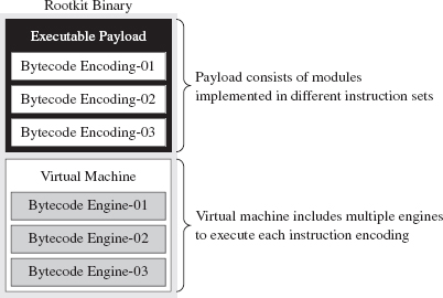
Figure 8.7

Yet another way to make things more difficult for an investigator would be to create a whole series of fake instructions that, at first glance, appear to represent legitimate operations but are actually ignored by the virtual machine. Then you can sprinkle the bytecode with this junk code to help muddy the water.

There’s a certain beauty to this countermeasure. Not only does the virtual machine strategy package our logic in a form that off-the-shelf disassemblers will fail to decipher, but also this sort of approach lends itself to features that tend to be easier to implement in a virtual runtime environment, like loading code dynamically. Dynamic loading is what facilitates pluggable runtime extensions, such that we can implement the rootkit proper as a small core set of features and then load additional modules as needed (see Figure 8.8) so that it can adapt to its surroundings.

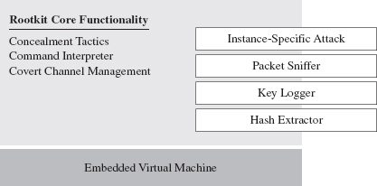
Figure 8.8

For instance, if you discover that the machine that you’ve gained a foothold on is running a certain vendor’s security software client, you can stream over a loadable module that’s explicitly designed to disarm and subvert the application. This saves you the trouble of having to compile the original rootkit with unnecessary functionality that will increase its footprint.

You may be thinking: “Loadable modules or no loadable modules, an embedded virtual machine is still going to make my rootkit into a whale of an executable, one that’s anything but inconspicuous.” After all, the Java Runtime Environment, with its many bells and whistles, can easily require more than 20 MB of storage. This is less of a problem than you might think. My own work in this area confirms that a serviceable virtual machine can be constructed that consumes less than 1 MB.

The Need for Custom Tools

Once a packing or encryption algorithm is known, an investigator will attempt to rely on automation to speed things up. Furthermore, tools will invariably be built to recognize that a certain armoring algorithm is in use so that the investigator knows which unpacker to use. The PEiD tool is an example. It can detect more than 600 different signatures in Windows PE executable files.¹⁴ PEiD has a “Hardcore Scan” mode that can be used to detect binaries packed with UPX.

I’ve said it before and I’ll say it again: Always use custom tools if you have the option. It robs the investigator of his ability to leverage automation and forces him, in turn, to create a custom tool to unveil your binary. This takes the sort of time and resources that anyone short of a state-sponsored player doesn’t have. He’s more likely to give up and go back to tweaking his LinkedIn profile.

The Argument Against Armoring

Now that we’ve made it through armoring, I have some bad news. Although armoring may successfully hinder the static analysis phase of an investigation, it also borders on a scorched earth approach. Remember, we want to be low and slow, to remain inconspicuous. If a forensic investigator unearths an executable with no strings and very few imports, he’ll know that he’s probably dealing with an executable that has been armored. It’s like a guy who walks into a jewelry store wearing sunglasses after dark: It looks really suspicious.

Looking suspicious is bad, because sometimes merely a hint of malice is enough for an assessor to conclude that a machine has been compromised and that the incident response guys need to be called. The recommended approach is to appear as innocuous and benign as possible. Let him perform his static analysis, let him peruse a dump of the machine instructions, and let him wrongfully conclude that there’s nothing strange going on. Nope, no one here but us sheep!

Some tools can detect armoring without necessarily having to recognize a specific signature. Recall that armoring is meant to foil disassembly by recasting machine code into a format that’s difficult to decipher. One common side-effect of this is that the machine code is translated into a seemingly random series of bytes (this is particularly true when encryption is being used). There are currently tools available, like Mandiant’s Red Curtain, that gauge how suspicious a file is based on the degree of randomness exhibited by its contents.¹⁵

Data Fabrication

Having issued the previous warning, if you must armor then at least camouflage your module to look legitimate. For example, one approach would be to decorate the stub application with a substantial amount of superfluous code and character arrays that will make anyone dumping embedded strings think that they’re dealing with some sort of obscure Microsoft tool:

Yet another trick involves the judicious use of a resource-definition script (.RC file), which is a text file that uses special C-like resource statements to define application resources. The following is an example of a VERSIONINFO resource statement that defines version-related data that we can associate with an executable.

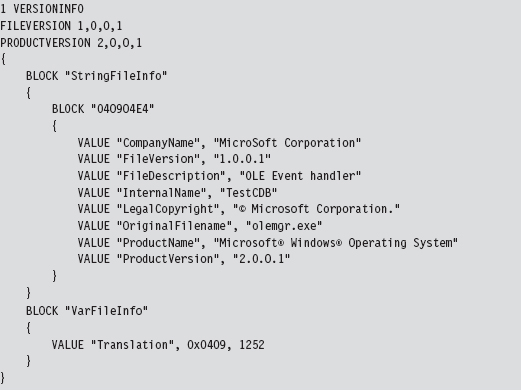
Once you’ve written the .RC file, you’ll need to compile it with the Resource Compiler (RC) that ships with the Microsoft SDK.

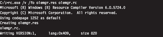
This creates a compiled resource (.RES) file. This file can then be stowed into an application’s .rsrc section via the linker. The easiest way to make this happen is to add the generated .RES file to the Resource Files directory under the project’s root node in the Visual Studio Solution Explorer. The final executable (e.g., olemgr.exe) will have all sorts of misleading details associated with it (see Figure 8.9).

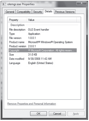
Figure 8.9

If you look at olemgr.exe with the Windows task manager or the Sysinternals Process Explorer, you’ll see strings like “OLE Event Handler” and “Microsoft Corporation.” The instinctive response of many a harried system administrator is typically something along the line of: “It must be one of those random utilities that shipped as an add-on when I did that install last week. It looks important (after all, OLE is core technology), so I better not mess with it.”

OEMs like Dell and HP are notorious for trying to push their management suites and diagnostic tools during installs (HP printer drivers in particular are guilty of this). These tools aren’t as well known or as well documented as the ones shipped by Microsoft. Thus, if you know the make and model of the targeted machine, you can always try to disguise your binaries as part of a “value-added” OEM package.

False-Flag Attacks

In addition to less subtle string decoration and machine code camouflage, there are regional and political factors that can be brought to the table. In early 2010, Google publicly announced¹⁷ that it had been the victim of a targeted attack aimed at its source code. Although authorities have yet to attribute the attacks to anyone in particular, the various media outlets seem to intimate that China is a prime suspect.

So, if you’re going to attack a target, you could launch your attack from machines in a foreign country (preferably one of the usual suspects) and then build your rootkit so that it appears to have been developed by engineers in that country. This is what’s known as a false-flag attack. If you’re fluent in the native language, it’s trivial to acquire a localized version of Windows and the corresponding localized development tools to establish a credible build environment.

Keep in mind that a forensic investigation will also scrutinize the algorithms you use and the way in which you manage your deployment to fit previously observed patterns of behavior. In the case of the Google attack, researchers observed a cyclic redundancy check routine in the captured malware that was virtually unknown outside of China.

Although this sort of masquerading can prove effective in misleading investigators, it’s also a scorched earth tactic. I don’t know about you, but nothing spells trouble to me like an unknown binary from another country. In contrast, if you realize that you’ve been identified as an intruder, or perhaps your motive is to stir up trouble on an international scale, you might want to throw something like this at the opposition to give them a bone to chew on.

Data Source Elimination: Multistage Loaders

This technique is your author’s personal favorite as it adheres to the original spirit of minimizing the quantity and quality of evidence that gets left behind. Rather than deliver the rootkit to the target in one fell swoop, the idea is to break down the process of deployment into stages in an effort to leave a minimal footprint on disk.

Here’s how multistage loaders work: Once a machine has been rooted, we leave a small application behind called a Stage-0 loader and configure the system somehow to launch this executable automatically so that we can survive a restart. This Stage-0 loader is a fairly primitive, hard-coded application whose behavior is fairly limited (see Figure 8.10). All it does is contact some remote machine over a covert channel and load yet another loader, called a Stage-1 loader.

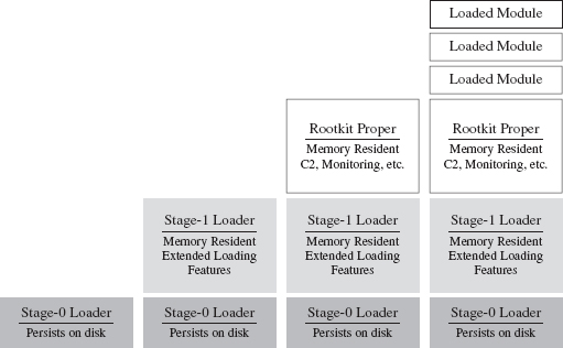
Figure 8.10

The Stage-1 loader is much larger, and as such it can offer a larger set of more sophisticated runtime features. Its configuration parameters aren’t hard-coded, like they are with the Stage-0 loader, and so it can adapt to a fluid environment with greater reliability. Furthermore, the Stage-1 loader is memory resident and doesn’t leave anything on disk (outside of the Windows page file).

Once the Stage-0 loader has situated the Stage-1 loader in memory, the Stage-1 loader will take program control and download the core rootkit. The rootkit will initiate C2 operations and possibly request additional extension modules as circumstances dictate. In the end, everything but the Stage-0 loader is memory resident. The Grugq has referred to this setup as an instance of data contraception.

It goes without saying that our Stage-0 and Stage-1 loaders must assume duties normally performed by the Windows loader, which resides in kernel space (e.g., mapping code into memory, resolving imported routine addresses, implementing relocation record fix-ups, etc.). Later on in the book, we’ll flesh out the details when we look at memory-resident software, user-mode loaders, and shellcode.

Defense In-depth

Here’s a point that’s worth repeating: Protect yourself by using these tactics concurrently. For instance, you could use the Mistfall strategy to implant a Stage-0 loader inside of a legitimate executable. This Stage-0 loader could be implemented using an arbitrary bytecode that’s executed by an embedded virtual machine, which has been developed with localized tools and salted with appropriate international character strings (so that it blends in sufficiently). So there you have it, see Table 8.2, a broad spectrum of anti-forensic strategies brought together in one deployment.

Table 8.2 Anti-Forensic Strategies

Strategy	Tactic
Data source elimination	Stage-0 loader
Data concealment	Inject the loader into an existing legitimate executable
Data transformation	Implement the loader as an arbitrary bytecode
Data fabrication	Build the loader with localized tools

8.3    Runtime Analysis

---

Static analysis often leads to runtime analysis. The investigator may want to get a more complete picture of what an executable does, confirm a hunch, or peek at the internals of a binary that has been armored. Regardless of what motivates a particular runtime analysis, the investigator will need to decide on what sort of environment he or she wants to use and whether he or she wishes to rely on automation as opposed to the traditional manual approach.

The Working Environment

It goes without saying that a runtime analysis must occur in a controlled setting. Launching a potentially malicious executable is like setting off a bomb. As far as malware testing grounds are concerned, a broad range of options has emerged (see Figure 8.11 and Table 8.3).

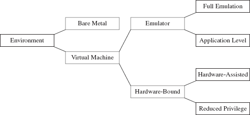
Figure 8.11

Some people still prefer the bare-metal approach where you take a physical host, known as the sacrificial lamb, with a smattering of other hosts (to provide the semblance of core network services) and put them all on a dedicated network segment that’s isolated from the rest of the world by an air gap.

Table 8.3 Types of Virtual Machine Environments

VM Environment	Example	URL
Full emulation	Bochs	http://bochs.sourceforge.net/
	QEMU	http://wiki.qemu.org/Main_Page
Application-level emulation	NTVDM	http://support.microsoft.com/kb/314106
	WoW64	http://msdn.microsoft.com/
Reduced-privilege guest VM	Java HotSpot VM	http://java.sun.com/docs/books/jvms/
	Virtual PC	http://www.microsoft.com/windows/virtual-pc/
Hardware-assisted VM	Hyper-V	http://www.microsoft.com/hyper-v-server/
	ESXi	http://www.vmware.com/

The operational requirements (e.g., space, time, electricity, etc.) associated with maintaining a bare-metal environment has driven some forensic investigators to opt for virtual machine (VM) setup. With one midrange server (24 cores with 128 GB of RAM), you can quickly create a virtual network that you can snapshot, demolish, and then wipe clean with a few mouse clicks.

Virtual machines come in two basic flavors:

  Emulators.

  Hardware-bound VMs.

An emulator is implemented entirely in software. It seeks to replicate the exact behavior of a specific processor or development platform. Full emulation virtual machines are basically user-mode software applications that think they’re a processor. They read in a series of machine instructions and duplicate the low-level operations that would normally be performed by the targeted hardware. Everything happens in user space. Needless to say, they tend to run a little slow.

There are also application-level emulators. We’ve seen these already under a different moniker. Application-level emulators are what we referred to earlier as runtime subsystems, or just “subsystem” for short. They allow an application written for one environment (e.g., 16-bit DOS or Windows 3.1 programs) to be run by the native environment (e.g., IA-32). Here, the goal isn’t so much to replicate hardware at the byte level as it is simply to get the legacy executable to run. As such, the degree of the emulation that occurs isn’t as fine grained.

On the other side of the fence are the hardware-bound virtual machines, which use the underlying physical hardware directly to execute their code. Though hardware-bound VMs have received a lot of press lately (because commodity hardware has progressed to the point where it can support this sort of functionality), the current generation is based on designs that have been around for decades. For example, back in the 1960s, IBM implemented hardware-bound virtual machine technology in its System/360 machines.

A reduced-privilege guest virtual machine is a hardware-bound virtual machine that executes entirely at a lower privilege (i.e., user mode). Because of performance and compatibility issues, these are sort of a dying breed.

The next step up from this is hardware-assisted virtual machines, which rely on a small subset of special machine instructions (e.g., Intel’s Virtualization Technology Virtual Machine Extensions, or VT VMX) to allow greater access to hardware so that a virtual machine can pretty much run as if it were loaded on top of bare metal.

In the case of hardware-assisted virtual machines, a special software component known as a hypervisor mediates access to the hardware so that several virtual machines can share resources. The hypervisor runs in its own ring of privilege (Ring −1, or root operating mode). Think of Ring −1 as Ring 0 with higher walls and reinforced concrete. Typically, one of the virtual machines will be designated as the management instance (Microsoft refers to this as the parent partition) and will communicate with the hypervisor to control the other virtual machines (see Figure 8.12). These other virtual machines, the ones under the sway of the parent partition, are known in Microsoft documents as child partitions.

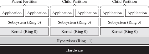
Figure 8.12

So, we have all these different types of testing environments. Which one is the best? The answer is that it depends. My goal in the last page or two has been to introduce you to some terms that you’ll see again. Ultimately, the environment that an investigator uses will depend on the type of runtime analysis that he’s going to use and the nature of the tools he’ll bring to the table. We’ll explore the trade-offs over the next few sections.

Manual Versus Automated Runtime Analysis

Manual runtime analysis requires the investigator to launch the unknown executable in an environment that he himself configures and controls. He decides which monitoring tools to use, the length of the test runs, how he’ll interact with the unknown binary, and what system artifacts he’ll scrutinize when it’s all over.

Manual runtime analysis is time intensive, but it also affords the investigator a certain degree of flexibility. In other words, he can change the nature of future test runs based on feedback, or a hunch, to extract additional information. If an investigator is going to perform a manual runtime analysis of an unknown executable, he’ll most likely do so from the confines of a bare-metal installation or (to save himself from constant re-imaging) a hardware-assisted virtual machine.

The downside of a thorough manual runtime analysis is that it takes time (e.g., hours or perhaps even days). Automated runtime analysis speeds things up by helping the investigator to filter out salient bits of data from background noise. Automated analysis relies primarily on forensic tools that tend to be implemented as either an application-level emulator or carefully designed scripts that run inside of a hardware-assisted virtual machine. The output is a formatted report that details a predetermined collection of behaviors (e.g., registry keys created, files opened, tasks launched, etc.).

The time saved, however, doesn’t come without a price (literally). Commercial sandboxes are expensive because they have a limited market and entail a nontrivial development effort. This is one reason why manual analysis is still seen as a viable alternative. An annual license for a single sandbox can cost you $15,000.¹⁸

Manual Analysis: Basic Outline

An investigator will begin a manual runtime analysis by verifying that all of the tools he needs have been installed and configured (see Figure 8.13). As I mentioned earlier, the benefit of the manual approach is that the investigator can use feedback from past trials to focus in on leads that look promising. As such, he may discover that he needs additional tools as the investigation progresses.

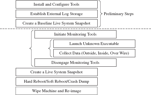
Figure 8.13

It also helps if any log data that gets generated is archived on an external storage location. Once the executable has run, the test machine loses its “trusted” status. The information collected during execution should be relocated to a trusted machine for a postmortem after the test run is over.

Next, the investigator will take a live snapshot of the test machine so that he has something that he can compare the final snapshot against later on (e.g., a list of running processes, loaded modules, open file handles, a RAM dump, etc.). This snapshot is very similar to the sort of data that would be archived during a live incident response. The difference is that the investigator has an idea of what sort of things he’ll be looking for in advance.

Once the baseline has been archived, the investigator will enable his monitoring tools (whatever they may be) and launch the unknown executable. Then he’ll interact with the executable, watch what it does from the inside, the impact that it has on its external surroundings, and capture any network traffic that gets generated. This phase can consume a lot of time, depending upon how much the investigator wants to examine the unknown binary’s runtime antics. If he’s smart, he’ll also take careful notes of what he does and the results that he observes.

When the investigator feels like he’s taken the trial run as far as he can, he’ll terminate the unknown executable and disable his monitoring tools. To help round things out, he’ll probably generate another live system snapshot.

Finally, the investigator will close up shop. He’ll yank the power cord outright, shut down the machine normally, or instigate a crash dump (perhaps as a last-ditch attempt to collect runtime data). Then he’ll archive his log data, file his snapshots, and rebuild the machine from the firmware up for the next trial run.

Manual Analysis: Tracing

One way the investigator can monitor an unknown application’s behavior at runtime is to trace its execution path. Tracing can be performed on three levels:

  System call tracing.

  Library call tracing.

  Instruction-level tracing.

System call tracing records the system routines in kernel space that an executable invokes. Though one might initially presume that this type of information would be the ultimate authority on what a program is up to, this technique possesses a couple of distinct shortcomings. First, and foremost, monitoring system calls doesn’t guarantee that you’ll capture everything when dealing with a user-mode executable because not every user-mode action ends up resolving to a kernel-mode system call. This includes operations that correspond to internal DLL calls.

Then there’s also the unpleasant reality that system calls, like Windows event messages, can be cryptically abstract and copious to the point where you can’t filter out the truly important calls from the background noise, and even then you can’t glean anything useful from them. Unless you’re dealing with a KMD, most investigators would opt to sift through more pertinent data.

Given the limitations of system call tracing, many investigators opt for library call tracing. This monitors Windows API calls at the user-mode subsystem level and can offer a much clearer picture of what an unknown executable is up to.

With regard to system call and library call tracing, various solid tools exist (see Table 8.4).

Table 8.4 Tracing Tools

Tool	Source
Logger.exe, Logviewer.exe	http://www.microsoft.com/whdc/devtools/WDK/default.mspx
Procmon.exe	http://technet.microsoft.com/en-us/sysinternals/bb896645.aspx
Procexp.exe	http://technet.microsoft.com/en-us/sysinternals/bb896653.aspx

Logger.exe is a little-known diagnostic program that Microsoft ships with its debugging tools (which are now a part of the WDK). It’s used to track the Windows API calls that an application makes. Using this tool is a cakewalk; you just have to make sure that the Windows debugging tools are included in the PATH environmental variable and then invoke logger.exe.

Behind the scenes, this tool does its job by injecting the logexts.dll DLL into the address space of the unknown executable, which “wraps” calls to the Windows API. By default, logger.exe records everything (the functions called, their arguments, return values, etc.) in an .LGV file, as in Log Viewer. This file is stored in a directory named LogExts, which is placed on the user’s current desktop. The .LGV files that logger.exe outputs are intended to be viewed with the logviewer.exe program, which also ships with the Debugging Tools for Windows package.

The ProcMon.exe tool that ships with the Sysinternals Suite doesn’t offer the same level of detail as Logger.exe, but it can be simpler to work with. It records activity in four major areas: the registry, the file system, network communication, and process management. Although ProcMon.exe won’t always tell you exactly which API was called, it will give you a snapshot that’s easier to interpret. It allows you to sort and filter data in ways that Logviewer.exe doesn’t.

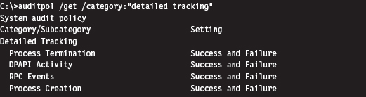
In addition to all of these special-purpose diagnostic tools, there are settings within Windows that can be toggled to shed a little light on things. For example, a forensic investigator can enable the Audit Process Tracking policy so that detailed messages are generated in the Security event log every time a process is launched. This setting can be configured at the command line as follows:

Once this auditing policy has been enabled, it can be verified with the following command:

At the finest level of granularity, there’s instruction tracing, which literally tracks what a module does at the machine-code level. This is the domain of debuggers and the like.

Manual Analysis: Memory Dumping

In addition to watching what an unknown executable does by tracing, the investigator can capture the internal runtime state of an executable by dumping its address space. The Autodump+ tool that ships with the WDK (i.e., adplus. vbs) is really just a glorified Visual Basic Script that wraps an invocation of the CDB.exe user-mode debugger. This is the Old Faithful of single-process memory dumping tools. It’s not as sexy as its more contemporary peers, but Autodump+ is dependable, and it’s maintained by the same company that sells the operating system that it targets.

Autodump+ can be invoked using the following batch script:

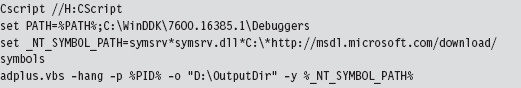
Let’s go through this line by line. The batch file begins by setting the default script interpreter to be the command-line incarnation (i.e., CScript), where output is streamed to the console. Next, the batch file sets the path to include the directory containing Autodump+ and configures the symbol path to use the Microsoft Symbol Server per Knowledge Base Article 311503. Finally, we get to the juicy part where we invoke Autodump+.

Now let’s look at the invocation of Autodump+. The command has been launched in hang mode; which is to say that we specify the –hang option in an effort to get the CDB debugger to attach noninvasively to a process whose PID we have provided using the –p switch. This way, the debugger can suspend all of the threads belonging to the process and dump its address space to disk without really disturbing that much. Once the debugger is done, it will disconnect itself from the target and allow the unknown executable to continue executing as if nothing had happened.

Because we invoked Autodump+ with the –o switch, this script will place all of its output files in the directory specified (e.g., D:\OutputDir). In particular, Autodump+ will create a subdirectory starting with the string “Hang_Mode_” within the output directory that contains the items indicated in Table 8.5.

Table 8.5 Autodump+ Output Files

Artifact	Description
.DMP file	A memory dump of the process specified
.LOG file	Detailed summary of the dumping process
ADPlus_report.txt	An overview of the runtime parameters used by ADPlus.vbs
Process_List.txt	A list of currently running tasks
CDBScripts directory	A replay of the dump in terms of debugger-level commands

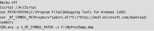
The .LOG file is a good starting point. If you need more info, then look at memory dump with the CDB.exe debugger:

Manual Analysis: Capturing Network Activity

In my own fieldwork, I’ve always started with local network monitoring by using TCPView.exe to identify overt network communication. Having identified the source of the traffic, I usually launch Process Explorer and Process Monitor to drill down into the finer details. If the TCP/UDP ports in use are those reserved for LDAP traffic (e.g., 389, 636), I might also monitor what’s going with an instance of ADInsight.exe. Though these tools generate a ton of output, they can be filtered to remove random noise and yield a fairly detailed description of what an application is doing.

The forensic investigator might also scan the test machine from the outside with an auditing tool like nmap to see if there’s an open port that’s not being reported locally. This trick can be seen as a network-based implementation of cross-view detection. For example, a rootkit may be able to hide a listening port from someone logged into the test machine, by using his own network driver, but the port will be exposed when it comes to an external scan.

Rootkits, by their nature, need to communicate with the outside world. You may be able to conceal network connections from someone sitting at the console, but unless you find a way to subvert the underlying network infrastructure (e.g., switches, routers, bridges, etc.), there’s very little you can do against packet capturing tools (see Table 8.6). This is why investigators, in addition to local network traffic monitoring, will install a sniffer to examine what’s actually going over the wire. There are several ways to do this in practice. They may use a dedicated span port, set up a network tap, or (if they’re really low end) insert a hub.

Table 8.6 Network Traffic Tools

Tool	Type	URL
TCPView	Local	http://technet.microsoft.com/en-us/sysinternals/
Tcpvcon	Local	http://technet.microsoft.com/en-us/sysinternals/
ADInsight	Local	http://technet.microsoft.com/en-us/sysinternals/
Wireshark	Remote	http://www.wireshark.org/
Network Monitor	Remote	http://www.microsoft.com/downloads/
nmap	Remote	http://nmap.org/

Automated Analysis

For some investigators, manual runtime analysis might as well be called “manual labor.” It’s monotonous, time consuming, and exhausting. Automated runtime analysis helps to lighten the load, so to speak, by allowing the investigator to circumvent all of the staging and clean-up work that would otherwise be required.

The virtual machine approach is common with regard to automated analysis. For example, the Norman Sandbox examines malware by simulating machine execution via full emulation.¹⁹ Everything that you’d expect (e.g., BIOS, hardware peripherals, etc.) is replicated with software. One criticism of this approach is that it’s difficult to duplicate all of the functionality of an actual bare-metal install.

The CWSandbox tool sold by Sunbelt Software uses DLL injection and detour patching to address the issues associated with full emulation. If the terms “DLL injection” and “detour patching” are unfamiliar, don’t worry, we’ll look at these in gory detail later on in the book. This isn’t so much an emulator as it is a tricked-out runtime API tracer. The CWSandbox filters rather than encapsulates. It doesn’t simulate the machine environment; the unknown executable is able to execute legitimate API calls (which can be risky, because you’re allowing the malware to do what it normally does: attack). It’s probably more appropriate to say that CWSandbox embeds itself in the address space of an unknown executable so that it can get a firsthand view of what the executable is doing.

In general, licensing or building an automated analysis tool can be prohibitively expensive. If you’re like me and on a budget, you can take Zero Wine for a spin. Zero Wine is an open-source project.²⁰ It’s deployed as a virtual machine image that’s executed by QEMU. This image hosts an instance of the Debian Linux distribution that’s running a copy of Wine. Wine is an application-level emulator (often referred to as a compatibility layer) that allows Linux to run Windows applications. If this sounds a bit recursive, it is. You essentially have an application-level emulator running on top of a full-blown machine emulator. This is done in an effort to isolate the executable being inspected.

Finally, there are online services like ThreatExpert,²¹ Anubis,²² and VirusTotal²³ that you can use to get a feel for what an unknown executable does. You visit a website and upload your suspicious file. The site responds back with a report. The level of detail you receive and the quality of the report can vary depending on the underlying technology stack the service has implemented on the back end. The companies that sell automated analysis tools also offer online submission as a way for you to test drive their products. I tend to trust these sites a little more than the others.

Composition Analysis at Runtime

If an investigator were limited to static analysis, packers and cryptors would be the ultimate countermeasure. Fortunately, for the investigator, he or she still has the option of trying to peek under the hood at runtime. Code may be compressed or encrypted, but if it’s going to be executed at some point during runtime, it must reveal itself as raw machine code. When this happens, the investigator can dump these raw bytes to a file and examine them. Hence, attempts to unpack during the static phase of analysis often lead naturally to tactics used at runtime.

Runtime unpackers run the gamut from simple to complicated (see Table 8.7).

Table 8.7 Unpacking Tools

Tool	Example	Description
Memory dumper	Autodump+	Simply dumps the current memory contents
Debugger plug-in	Universal PE Unpacker	Allows for finer-grained control over dumping
Code-buffer	PolyUnpack	Copies code to a buffer for even better control
Emulator-based	Renovo	Detects unpacking from within an emulator
W-X monitor	OmniUnpack	Tracks written-then-executed memory pages

At one end of the spectrum are memory dumpers. They simply take a process image and write it to disk without much fanfare.

Then there are unpackers that are implemented as debugger plug-ins so that the investigator has more control over exactly when the process image is dumped (e.g., just after the unpacking routine has completed). For instance, IDA Pro ships with a Universal PE Unpacker plug-in.²⁴

The code-buffer approach is a step up from the average debugger plug-in. It copies instructions to a buffer and executes them there to provide a higher degree of control than that of debuggers (which execute in place). The Poly-Unpack tool is an implementation of this idea.²⁵ It starts by decomposing the static packed executable into code and data sections. Then it executes the packed application instruction by instruction, constantly observing whether the current instruction sequence is in the code section established in the initial step.

Emulator-based unpackers monitor a packed executable from outside the matrix, so to speak, allowing the unpacker to attain a somewhat objective frame of reference. In other words, they can watch execution occur without becoming a part of it. Renovo is an emulator-based unpacker that is based on QEMU.²⁶ It extends the emulator to monitor an application for memory writes in an effort to identify code that has been unpacked.

W-X monitors look for operations that write bytes to memory and then execute those bytes (i.e., unpack a series of bytes in memory so that they can be executed). This is normally done at the page level to minimize the impact on performance. The OmniUnpack tool is an instance of a W-X monitor that’s implemented using a Windows KMD to track memory access.²⁷

8.4    Subverting Runtime Analysis

---

The gist of the last section is that the investigator will be able to observe, one way or another, everything that we do. Given this, our goal is twofold:

  Make runtime analysis less productive.

  Do so in a way that won’t raise an eyebrow.

Believe it or not, there’s a whole segment of the industry devoted to foiling runtime analysis: software protection. There are reputable commercial software tools like Themida²⁸ and Armadillo²⁹ that are aimed to do just that. Yep, one person’s malware armor is another person’s software protection. Just like one person’s reversing is another person’s runtime analysis (Figure 8.14).

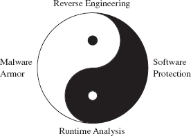
Figure 8.14

However, I think I should mention that software protection, unlike rootkit armor, is allowed to be conspicuous. A protected software application isn’t necessarily trying to blend in with the woodwork. It can be as brazen as it likes with its countermeasures because it has got nothing to hide.

In this section, we’ll look at ways to defeat tracing, memory dumping, and automated runtime analysis. Later on in the book, when we delve into covert channels, we’ll see how to undermine network packet monitoring.

Tracing Countermeasures

To defeat tracing, we will fall back on core anti-forensic strategies (see Table 8.8). Most investigators will start with API tracing because it’s more expedient and only descend down into the realm of instruction-level tracing if circumstances necessitate it. Hence, I’ll begin by looking at ways to subvert API tracing and then move on to tactics intended to frustrate instruction-level tracing.

Table 8.8 Tracing Countermeasures

Strategy	Example Tactics
Data concealment	Evading detour patches
Data transformation	Obfuscation
Data source elimination	Anti-debugger techniques, multistage loaders

API Tracing: Evading Detour Patches

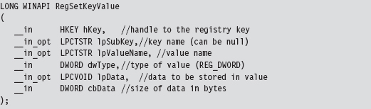
Looking at Figure 8.15, you’ll see the standard execution path that’s traversed when a user-mode application (i.e., the unknown application) invokes a standard Windows API routine like RegSetKeyValue(). Program control gradually makes its way through the user-mode libraries that constitute the Windows subsystem and then traverse the system call gate into kernel mode via the SYSENTER instruction in the ntdll.dll module.

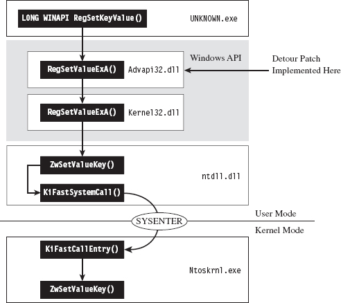
Figure 8.15

One way to trace API invocations is to intercept them at the user-mode API level. Specifically, you modify the routines exported by subsystem DLLs so that every time an application calls a Windows routine to request system services, the invocation is logged.

The mechanics of intercepting program control involve what’s known as detour patching (see Figure 8.16). The term is fairly self-explanatory. You patch the first few bytes of the targeted Windows API routine with a jump instruction so that when your code calls the function, the path of execution is re-routed through a detour that logs the invocation (perhaps taking additional actions if necessary). Tracing user-mode API calls using detour patches has been explored at length by Nick Harbour.³⁰

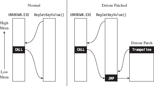
Figure 8.16

When the detour is near completion, it executes the code in the original API routine that was displaced by the jump instruction and then sends the path of execution back to the API routine. The chunk of displaced code, in addition to the jump that sends it back to the original API routine, is known as a trampoline (e.g., executing the displaced code gives you the inertia you need before the jump instruction sends you careening back to the API call).

Tracing with detour patches has its advantages. You can basically track everything that a user-mode application does with regard to calling exported library calls. The bad news is that it’s also straightforward to subvert. You simply sidestep the jump instruction in the API routine by executing your own trampoline (see Figure 8.17).

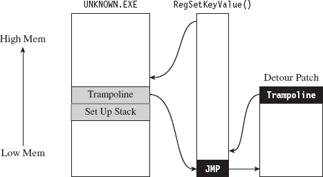
Figure 8.17

Put another way, you re-create the initial portion of the API call so that you can skip the detour jump that has been embedded in the API call by the logging code. Then, instead of calling the routine as you normally would, you go directly to the spot following the detour jump so that you can execute the rest of the API call as you normally would.

Here’s how this would look implemented in code:

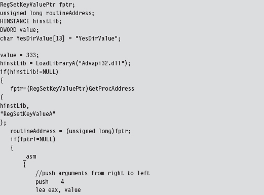
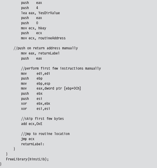
This code invokes the following API call:

In this code, we build our own stack frame, then instead of calling the API routine as we normally would (using the CALL assembly code instruction), we manually execute the first few bytes of the routine and then jump to the location in the API’s code that resides just after these first few bytes. Piece of cake!

Naturally, there’s a caveat. Whereas this may work like a charm against detour patches, using this technique to undermine a tool like ProcMon.exe from the confines of a user-mode application won’t do much good. This is because ProcMon.exe uses a KMD to track your code. You heard correctly, this tool goes down into the sub-basement of Windows, where it’s granted a certain degree of protection from malicious user-mode apps and can get a better idea of what’s going on without interference.

You may be thinking: “But, but … Reverend Bill, I don’t see any .sys files associated with ProcMon.exe in the Sysinternals Suite directory. How does this program execute in kernel mode?”

That’s an excellent question. ProcMon.exe is pretty slick in this regard. It contains an embedded KMD that it dynamically unpacks and loads at runtime, which is why you need membership in the local administrator group to run the program (see Figure 8.18). From its vantage point in kernel space, the KMD can latch on to the central data structures, effectively monitoring the choke point that most system calls must traverse.

In a way, evading detour patches is much more effective when working in kernel space because it’s much easier to steer clear of central choke points. In kernel space there’s no call gate to skirt; the system services are all there waiting to be invoked directly in a common plot of memory. You just set up a stack frame and merrily jump as you wish.

To allow a user-mode application to bypass monitoring software like ProcMon.exe, you’d need to finagle a way for invoking system calls that didn’t use the conventional system call gate. Probably the most direct way to do this would be to establish a back channel to kernel space. For example, you could load a driver in kernel space that would act as a system call proxy. But even then, you’d still be making DeviceIoControl() calls to communicate with the driver, and they would be visible to a trained eye.

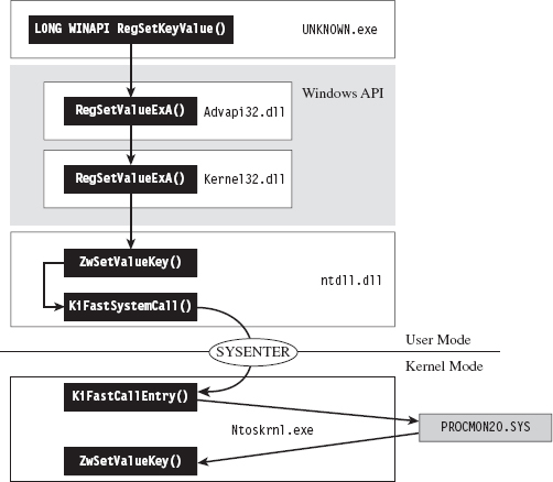
Figure 8.18

One way around this would be to institute a more passive covert channel. Rather than the user-mode application explicitly initiating communication by making an API call (e.g., DeviceIOControl()), why not implement a rogue GDT entry that the application periodically polls. This would be the programmatic equivalent of a memory-resident dead drop where it exchanges messages with the driver.

API Tracing: Multistage Loaders

The best way to undermine API logging tools is to avoid making an API call to begin with. But this isn’t necessarily reasonable (although, as we’ll see later on in the book, researchers have implemented this very scheme). The next best thing would be to implement the sort of multistage loader strategy that we discussed earlier on.

The idea is that the unknown application that you leave behind does nothing more than to establish a channel to load more elaborate memory-resident components. Some researchers might try to gain additional information by running the loader in the context of a sandbox network to get the application to retrieve its payload so they can see what happens next. You can mislead the investigator by identifying nonproduction loaders and then feeding these loaders with a harmless applet rather than a rootkit.

Instruction-Level Tracing: Attacking the Debugger

If an investigator isn’t content with an API-level view of what’s happening, and he has the requisite time on his hands, he can launch a debugger and see what the unknown application is doing at the machine-instruction level.

To attack a debugger head-on, we must understand how it operates. Once we’ve achieved a working knowledge of the basics, we’ll be in a position where we can both detect when a debugger is present and challenge its ability to function.

Break Points

A break point is an event that allows the operating system to suspend the state of a module (or, in some cases, the state of the entire machine) and transfer program control over to a debugger. On the most basic level, there are two different types of break points:

  Hardware break points.

  Software break points.

Hardware break points are generated entirely by the processor such that the machine code of the module being debugged need not be altered. On the IA-32 platform, hardware break points are facilitated by a set of four 32-bit registers referred to as DR0, DR1, DR2, and DR3. These four registers store linear addresses. The processor can be configured to trigger a debug interrupt (i.e., INT 0×01, also known as #DB trap) when the memory at one of these four linear addresses is read, written to, or executed.

Software break points are generated by inserting a special instruction into the execution path of a module. In the case of the IA-32 platform, this special instruction is INT 0×03 (also referred to as the #BP trap), which is mapped to the 0×CC opcode. Typically, the debugger will take some existing machine instruction and replace it with 0×CC (padded with Intel CPU instruction (NOPs), depending on the size of the original instruction). When the processor encounters this instruction, it executes the #BP trap, and this invokes the corresponding interrupt handler. Ultimately, this will be realized as a DEBUG_EVENT that Windows passes to the debugger. The debugger, having called a routine like WaitForDebugEvent() in its main processing loop, will be sitting around waiting for just this sort of occurrence. The debugger will then replace the break point with the original instruction and suspend the state of the corresponding module.

Once a break point has occurred, it will usually be followed by a certain amount of single-stepping. Single-stepping allows instructions to be executed in isolation. It’s facilitated by the Trap flag (TF; the 9th bit of the EFLAGS register). When TF is set, the processor generates a #DB trap after each machine instruction is executed. This allows the debugger to implement the type of functionality required atomically to trace the path of execution, one instruction at a time.

Detecting a User-Mode Debugger

The official Windows API call, IsDebuggerPresent(), is provided by Microsoft to indicate if the current process is running in the context of a user-mode debugger.

This routine returns zero if a debugger is not present. There isn’t much to this routine; if you look at its disassembly you’ll see that it’s really only three or four lines of code:

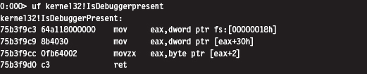
One way to undermine the effectiveness of this call is to hook a program’s IAT so that calls to IsDebuggerPresent() always returns a zero value. You can circumvent this defense by injecting this routine’s code directly into your executable:

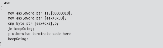
If you look more closely at this code and walk through its instructions, you’ll see that this code is referencing a field in the application’s PEB.

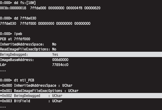
Thus, a more decisive way to subvert this approach is simply to edit the BeingDebugged field in the PEB. In fact, there are debuggers that will do just that in an effort to fake out malware.

This leaves us looking for something a little more robust. It just so happens that there’s an API call, CheckRemoteDebuggerPresent(), that detects if the current process is being examined by a debugger that resides in a separate parallel process (as opposed to the IsDebuggerPresent() call, which detects if the current process is running inside of a debugger process).

By tracing the execution path of this call, we can see that it ends up invoking a routine in the kernel: nt!NtQueryInformationProcess(). This undocumented kernel-space routine checks the DebugPort field in the EPROCESS structure associated with the process. If this field is nonzero, it indicates that a debugger is present.

One might suspect that because the DebugPort field is in kernel space that it might be better protected from manipulation by Ring 3 debuggers. Unfortunately this isn’t the case. It’s pretty straightforward simply to patch this API code in user mode so that it wrongfully indicates the absence of a debugger.

Okay, so let’s look at ways to detect a debugger without relying on API calls or global flags. One way is randomly to insert a break-point instruction into code. Normally, in the absence of a debugger, an exception will be raised that your code will need to catch. But, when a debugger latches onto your code, it will take over this responsibility and skip your manual exception handling.

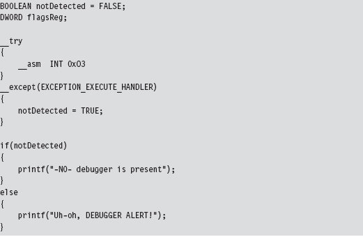
Yet another way to detect a user-mode debugger without relying on API calls or global flags is to use the Read Time Stamp Counter machine instruction (e.g., RDTSC). This instruction is essentially a lightweight mechanism for timing the processor. It returns the number of CPU ticks since system restart, where a tick is some processor-dependent quantum of time (e.g., of the order nanoseconds). This value is represented as a 64-bit quantity whose high-order DWORD is placed in the EDX register and whose lower-order DWORD is placed in the EAX register.

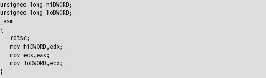
The basic idea here is that an interactive debugger will generate noticeable pauses in the execution path as the investigator suspends the application to poke around. If you quietly sprinkle your code with timing checks, you may be able to detect these pauses.

Detecting a Kernel-Mode Debugger

A KMD can execute the following function call to determine if a kernel-mode debugger is active.

This routine refreshes and then returns the value of KD_DEBUGGER_NOT_PRESENT global kernel variable.

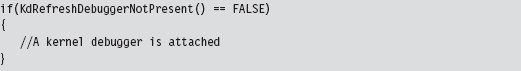
If you wanted to, you could query this global variable directly; it’s just that its value might not reflect the machine’s current state:

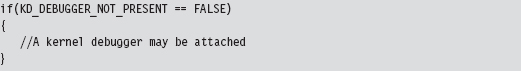
Detecting a User-Mode or a Kernel-Mode Debugger

Regardless of whether a program is being examined by a user-mode debugger or a kernel-mode debugger, the TF will be used to implement single-stepping. Thus, we can check for a debugger by setting the TF. When we update the value of the EFLAGS register with the POPFD instruction, as shown below, a #DB trap will automatically be generated. If a debugger is already present, it will swallow the trap, and our exception handling code will never be invoked.

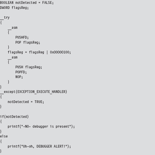
As you may have suspected, there’s a caveat to this approach. In particular, some debuggers will only be detected if the detection code is literally being stepped through (as opposed to the debugger merely being present).

Detecting Debuggers via Code Checksums

Software break points necessitate the injection of foreign opcodes into the original stream of machine instructions. Hence, another way to detect a debugger is to have your code periodically scan itself for modifications. This is essentially how Microsoft implements kernel patch protection (KPP). Be warned that this sort of operation is expensive and can significantly slow things down. The best way to use this tactic is to pick a subset of routines that perform sensitive operations and then, at random intervals, verify their integrity by drawing on a pool of potential checksum procedures that are chosen arbitrarily. Mixed with a heavy dose of obfuscation, this can prove to be a formidable (though imperfect) defense.

One way around checksum detection is to rely on hardware break points. A user-mode application can attempt to counter this maneuver by using the GetThreadContext() API call.

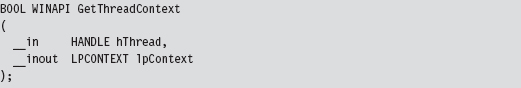
This call populates a CONTEXT structure for the thread whose handle is passed as an input parameter to the routine. If you peruse the Winnt.h header file, you’ll see that this structure contains, among other things, the contents of the hardware debug registers.

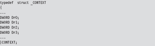
The Argument Against Anti-Debugger Techniques

If you can detect a debugger, then you’re also in a position to spring an ambush on it. The name of the game from this point onward is subtlety. The central goal of a rootkit is to evade detection or at least appear outwardly harmless. If an investigator is debugging your executable and it crashes his debugger, it looks bad. It’s like a cop performing an interrogation: He may not know what you’re hiding, but he does know that you’re being extremely evasive. This, in and of itself, will mark you as a potential perp.

Likewise from the standpoint of an investigator who’s on a budget and doing a preemptive assessment, it may be enough that he’s found a suspect. He might not necessarily care to know exactly what an unknown executable does, but if the executable is acting like it’s got something to hide, the investigator may decide that he’s been rooted and it’s time to call in the incident responders.

This is why I don’t like anti-debugger techniques. Yes, I’ll admit, some of the countermeasures are very clever. At the same time, they can be conspicuous and that’s not good.

Instruction-Level Tracing: Obfuscation

The goal of obfuscation is to alter an application so that:

  Its complexity (potency) is drastically amplified.

  Its intent is difficult to recover (i.e., the obfuscation is resilient).

  It still functions correctly.

Obfuscation can be performed at the source-code level or machine-code level. Both methods typically necessitate regression testing to ensure that obfuscation hasn’t altered the intended functionally of the final product.

Obfuscation at machine-code level is also known as code morphing. This type of obfuscation uses random transformation patterns and polymorphic replacement to augment the potency and resilience of an executable. Code morphing relies on the fact that the IA-32 instruction set has been designed such that it’s redundant; there’s almost always several different ways to do the same thing. Machine-level obfuscators break up a program’s machine code into small chunks and randomly replace these chunks with alternative instruction snippets. Strongbit’s Execryptor package is an example of an automated tool that obfuscates at the machine level.³²

Obfuscating at the source-code level is often less attractive because it affects the code’s readability from the standpoint of the developer. I mean, the idea behind obfuscation is to frustrate the forensic investigator, not the code’s original architect! This problem can be somewhat mitigated by maintaining two source trees: one that’s unprocessed (which is what gets used on a day-to-day basis) and another that’s been obfuscated. Unlike machine-level obfuscation, source-level obfuscation is sometimes performed manually. It’s also easier to troubleshoot if unexpected behavior crops up.

When it comes to obfuscation, there are tactics that can be applied to code and tactics that can be applied to data.

Obfuscating Application Data

Data can be altered with respect to how it is

  Encoded.

  Aggregated.

  Ordered.

Data encoding determines how the bits that make up a variable are used to represent values. For example, take a look at the following loop:

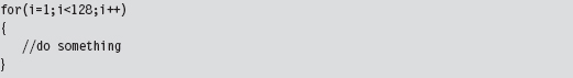
An investigator looking at this code will see something like:

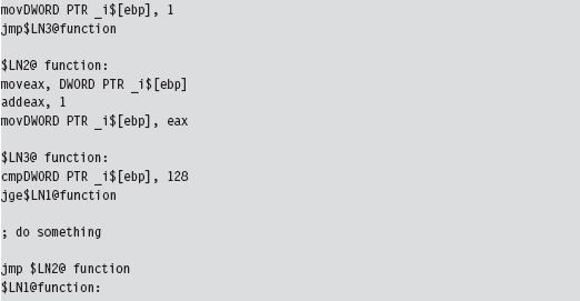
Changing the encoding of the loop index by shifting 2 bits to the left obscures its intuitive significance and makes life more difficult for someone trying to understand what’s going on.

Granted, this example is trivial. But it should give you an idea of what I mean with regard to modifying the encoding of a variable.

Data aggregation specifies how data is grouped together to form compound data types. In general, the more heavily nested a structure is, the harder it is to enumerate its constituents. Thus, one approach that can be used to foil the forensic investigator is to merge all of a program’s variables into one big unified superstructure.

Data ordering controls how related data is arranged in memory. Array restructuring is a classic example of obfuscation that alters how data is ordered. For example, you could interleave two arrays so that their elements are interspersed throughout one large array.

Obfuscating Application Code

Aside from runtime encryption or bytecode transformations, many code obfuscation techniques focus on altering the control flow of an application. The goal of these techniques is to achieve excess; either attain a state where there is no abstraction or attain a state where there is too much abstraction. Complexity becomes an issue at both ends of the architectural spectrum. To this end, the following tactics can be used:

  Inlining and outlining.

  Reordering operations.

  Stochastic redundancy.

  Use exception handling to transfer control.

  Code interleaving.

  Centralized function dispatching.

Inlining is the practice of replacing every invocation of a function with the function’s body. This way, the program can avoid the overhead of building a stack frame and jumping around memory. Inlining is a fairly standard optimization technique that trades off size for speed. Although the final executable will be faster, it will also be larger. This is a handy technique. It requires very little effort (usually toggling the compiler configuration option) but at the same time yields dividends because it destroys the procedural structure that high-level programming languages strive to impose.

Outlining is the flip side of the coin. It seeks to consolidate recurring snippets of program logic into dedicated functions in an effort to trade off space for time. The program will require less space, but it will take more time to run due to the overhead of making additional function calls. Anyone who’s worked with embedded systems, where memory is a scarce commodity, will immediately recognize this tactic. Taken to excess, this train of thought makes every statement into its own function call. If inlining results in no functions, outlining results in nothing but functions. Both extremes can confuse the investigator.

Reordering operations rely on the fact that not all statements in a function are sequentially dependent. This technique is utilized by identifying statements that are relatively independent of one another and mixing them up as much as possible. For added effect, reordering can be used in conjunction with interleaving (which will be described shortly). However, because this technique has the potential to cause a lot of confusion at the source-code level, it’s recommended that instruction reordering be performed at the machine-code level.

Anyone who has seen the 1977 kung fu movie entitled Golden Killah (part of the Wu Tang Forbidden Treasures series) will appreciate stochastic redundancy. In the movie, a masked rebel plagues local officials and eludes capture, seeming at times to defy death and other laws of nature. At the end of the film, we discover that there are actually dozens of rebels, all wearing the same outfit and the same golden mask. The idea behind this software technique is similar in spirit: create several slightly different versions of the same function and then call them at random. Just when the forensic investigator thinks that he’s nailed down a routine, it pops up unexpectedly from somewhere else.

Most developers are taught to use exception handling in a certain way. What our instructors typically fail to tell us is that exceptions can be used to perform abrupt global leaps between functions. Far jumps of this nature can make for painfully subtle transfers of program control, particularly when the jump appears to be a side effect rather than an official re-routing of the current execution path. This is one scenario where floating-point exceptions actually come in handy.

Code interleaving is carried out by taking two or more functions, separating their constituent statements, and merging them into a single routine by tightly weaving their statements together. The best way to see this is visually (see Figure 8.19). The key to reconnecting the individual statements back together into their respective routines is the use of opaque predicates.

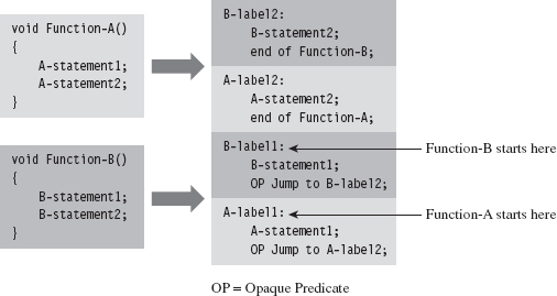
Figure 8.19

A predicate is just a conditional statement that evaluates to true or false. An opaque predicate is a predicate for which the outcome is known in advance, which is to say that it will always return the same result, even if it looks like it won’t. For example:

is an opaque predicate that’s always false.

Opaque predicates are essentially unconditional jumps that look like conditional jumps, which is what we want because we’d like to keep the forensic investigator off balance and in the dark as much as possible.

One way to augment code interleaving is to invoke all of the routines through a central dispatch routine. The more functions you merge together, the better. In the extreme case, you’d merge all of the routines in an executable through a single dispatch routine (which, trust me, can be very confusing). This centralized invocation strategy is the basic idea behind Armadillo’s Nanomite technology.³³

The dispatch routine maintains its own address table that maps return addresses to specific functions. This way, the dispatcher knows which routine to map to each caller. When a routine is invoked, the code making the invocation passes its return address on the stack. The dispatch routine examines this return address and references its address table to determine which function to re-route program control to (see Figure 8.20). In the eyes of the forensic investigator, everyone seems to be calling the same routine regardless of what happens.

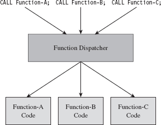
Figure 8.20

Hindering Automation

If a rootkit detects that it’s running within a virtual environment, it can alter its behavior to limit the amount of information that it discloses. This is one reason why many forensic investigators still prefer using a bare-metal lab environment. As in the case of a debugger, subverting an automated tool like an emulator comes down to two subtasks:

  Detecting the automated environment.

  Taking actions that undermine the effectiveness of the environment.

Building an emulator is no small job, which is one reason why you don’t see that many noncommercial implementations. The developers worked so hard that they want to recoup on their investment. Not to mention that there are literally hundreds of obscure routines that must be implemented in order for the unknown executable to behave as if it was executing in an actual subsystem. Therein resides a potential weak spot.

Implementing a perfect application-level emulator essentially entails reconstructing all of the functionality of a genuine application subsystem. Every possible execution path through the user-level API has to be replicated. The problem is that few automated tools are perfect. Hence, one way to detect a sandbox is intentionally to invoke an API call with incorrect parameters to see if the execution environment will return the corresponding error code. Some emulators are too lazy to re-create all of the requisite parameter checking, and this is their downfall.

The same sort of logic follows for full system emulators. Emit a few of the more obscure machine instructions and see what happens. Try to elicit exceptional behavior and then watch carefully for the appropriate response (or lack of response).

On Windows, child partitions running on top of the Hyper-V hypervisor layer almost always have special integration services running (see Table 8.9). These are easy to check for using the QueryServiceStatusEx() or RegOpenKeyEx() API calls and are a dead giveaway.

Table 8.9 Hyper-V Integration Service Routines

Service	Invocation Path
vmickvpexchange	Vmicsvc.exe (feature Kvpexchange)
vmicshutdown	Vmicsvc.exe (feature Shutdown)
vmicheartbeat	Vmicsvc.exe (feature Heartbeat)
Vmictimesync	Vmicsvc.exe (feature TimeSync)
Vmicvss	Vmicsvc.exe (feature VSS)

Once you’ve detected that your code is running in the confines of an automated system, your response should be measured. One avenue of approach is simply to wait out the emulator with some sort of time delay. That is, most emulators will exit after a certain point if they fail to detect suspicious behavior.

Obviously, the automated tool can’t execute forever: At some point, it has got to decide that it has executed its target long enough and call it a day. This tactic has proved successful in the field. You can augment it by having your code make a few innocent looking perfunctory API calls to give the impression that you’ve got nothing to hide. Candygram for Mongo!

Countering Runtime Composition Analysis

If an investigator gets the impression that you’ve armored your application, he may try to find that one magic spot in your code where the executable transforms itself back into naked machine instructions and then dump these naked bytes to disk. The goal of runtime encoding is to deny the investigator the ability to do so.

The ultimate solution would be some sort of homomorphic encryption scheme, where a computational engine processes encrypted inputs and generates encrypted output without ever decrypting the data. In English, you could design a program that’s encrypted even while it’s being executed. IBM has done some work in this area,³⁴ and DARPA has also demonstrated some interest.³⁵ So far, no one has come up with a reasonable algorithm.³⁶

A more mild, and feasible, variation of this idea is the shifting decode frame (also referred to as the running line). The basic idea is to keep the amount of code decrypted at any one point in time to a bare minimum so that it can’t be dumped all at once. Obviously, key management becomes an issue in this instance. This topic has been addressed at length by researchers who focus on what’s been dubbed white-box cryptography.³⁷

If you prefer to dispense with the rocket science altogether, a much more practical implementation along the same line would be to use an embedded virtual machine that supports multiple instruction encodings concurrently. This is the type of defense that software protectors like Themida use. It’s not perfect, but it does raise the bar significantly in terms of the effort that will be required to decipher the resulting memory dump. If the investigator wants to dump your virtual machine bytecode, fine. Give him the software equivalent of the Mayan hieroglyphs.

8.5    Conclusions

---

We started this chapter with the standard song-and-dance that is static executable analysis. As we saw, if a preemptive assessment were limited to static analysis, countermeasures like armoring would be all that we’d need to throw a monkey wrench into the process. Keep in mind, however, that our requirement to remain low and slow means that armoring must be done in such a manner that it doesn’t overtly appear to be armoring. Hence, we must combine armoring with other anti-forensic strategies to achieve defense in-depth (see Figure 8.21).

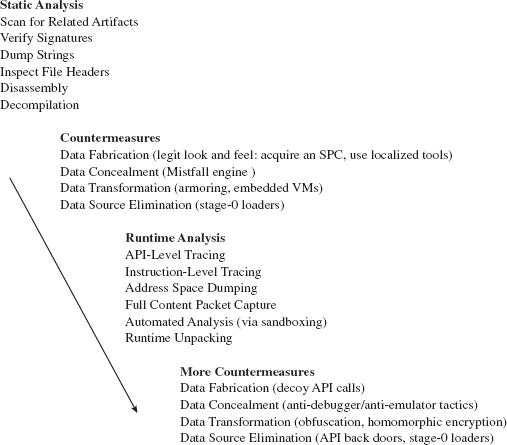
Figure 8.21

Countermeasures like armoring lead naturally to the analyst performing runtime executable analysis in an effort to get the unknown binary to unveil itself and disclose information related to its behavior during execution. In addition to conventional tracing utilities, the investigator may rely on automated sandboxes to save time and full-blown machine emulators to increase his level of control.

Yet even runtime analysis can be foiled. API tracing utilities can be sidestepped through back doors and the deployment of multistage loaders. Instruction-level tracing can be hindered through obfuscation and embedded virtual machines. Attempts to automate can be detected and quietly sabotaged. For every analytic tool that an investigator throws at us during his assessment, we can institute barriers that misdirect and complicate.

In the end, however, all of this fuss may prove unnecessary.

Years ago I heard an ex-convict claim that the best way to outsmart a prison guard is never to get incarcerated to begin with. He’s got a point, that guy. The same sort of logic holds true with regard to rootkits. I’ve devoted this entire chapter to the description of techniques you can use to make life difficult for an investigator who’s dissecting an unknown executable as a part of a preemptive disk analysis. However, these techniques only go so far. Depending on the investigator’s level of paranoia, the very fact that the investigator has discovered an unknown executable may be enough to signal an intrusion. When this happens, your campaign has failed because the primary goal of a rootkit is to allow you to remain undetected.

Thus, the definitive way to counter a disk analysis, and a subsequent executable analysis, is never to end up on disk to begin with. In other words, I’m talking about staying memory resident. This leads us to the next chapter…

 

---

  1. http://www.foundstone.com/us/resources/proddesc/bintext.htm.

  2. http://www.microsoft.com/whdc/system/platform/firmware/PECOFF.mspx.

  3. http://www.magma.ca/~wjr/.

  4. http://www.ollydbg.de/.

  5. http://www.hex-rays.com/idapro/.

  6. http://www.heaventools.com/.

  7. http://www.ul.com/global/eng/pages/corporate/aboutul/.

  8. http://yodap.sourceforge.net/download.htm.

  9. J. Riordan and B. Schneier, “Environmental Key Generation towards Clueless Agents.” In G. Vigna (ed.), Mobile Agents and Security, Springer-Verlag, 1998, pp. 15–24.

10. E. Filiol (May 2005). “Strong Cryptography Armoured Computer Viruses Forbidding Code Analysis: The Bradley Virus.” In Paul Turner & Vlasti Broucek (eds.), EICAR Best Paper Proceedings, 2005, pp. 216–227, ISBN 87-987271-7-6.

11. http://upx.sourceforge.net/.

12. Mental Driller, “How I made MetaPHOR and what I’ve learnt,” 29A, Volume 6, http://www.29a.net/.

13. http://www.oreans.com/codevirtualizer.php.

14. http://www.peid.info/.

15. http://www.mandiant.com/products/free_software/red_curtain/.

16. http://vxheavens.com/lib/vzo21.html.

17. http://googleblog.blogspot.com/2010/01/new-approach-to-china.html.

18. http://www.sunbeltsoftware.com/Malware-Research-Analysis-Tools/Sunbelt-CWSandbox/.

19. http://www.norman.com/technology/norman_sandbox/.

20. http://sourceforge.net/projects/zerowine/.

21. http://www.threatexpert.com.

22. http://anubis.iseclab.org.

23. http://www.virustotal.com.

24. http://www.hex-rays.com/idapro/unpack_pe/unpacking.pdf.

25. http://www.acsac.org/2006/abstracts/122.html.

26. http://www.andrew.cmu.edu/user/ppoosank/papers/renovo.pdf.

27. http://www.acsac.org/2007/papers/151.pdf.

28. http://www.oreans.com/themida.php.

29. http://www.siliconrealms.com/armadillo_engine.shtml.

30. Nick Harbour, Win At Reversing, Black Hat USA 2009.

31. http://www.nsa.gov/business/programs/tapo.shtml.

32. http://www.strongbit.com/execryptor.asp.

33. http://www.ring3circus.com/rce/armadillo-nanomites-and-vectored-exception-handling/.

34. http://domino.research.ibm.com/comm/research_projects.nsf/pages/security.homoenc.html.

35. https://www.fbo.gov/utils/view?id=11be1516746ea13def0e82984d39f59b.

36. http://www.schneier.com/blog/archives/2009/07/homomorphic_enc.html.

37. http://homes.esat.kuleuven.be/~bwyseur/research/wbc.php.