Table of Contents for
The Rootkit Arsenal: Escape and Evasion in the Dark Corners of the System, 2nd Edition
 The Rootkit Arsenal: Escape and Evasion in the Dark Corners of the System, 2nd Edition
Published by
Jones & Bartlett Learning, 2012
The Rootkit Arsenal: Escape and Evasion in the Dark Corners of the System, 2nd Edition
Published by
Jones & Bartlett Learning, 2012
- Cover
- Title Page
- Copyright
- The Rootkit Arsenal: Escape and Evasion in the Dark Corners of the System
- Contents
- Preface
- Part I: Foundations
- Chapter 1 Empty Cup Mind
- Chapter 2 Overview of Anti-Forensics
- Chapter 3 Hardware Briefing
- Chapter 4 System Briefing
- Chapter 5 Tools of the Trade
- Chapter 6 Life in Kernel Space
- Part II: Postmortem
- Chapter 7 Defeating Disk Analysis
- Chapter 8 Defeating Executable Analysis
- Part III: Live Response
- Chapter 9 Defeating Live Response
- Chapter 10 Building Shellcode in C
- Chapter 11 Modifying Call Tables
- Chapter 12 Modifying Code
- Chapter 13 Modifying Kernel Objects
- Chapter 14 Covert Channels
- Chapter 15 Going Out-of-Band
- Part IV: Summation
- Chapter 16 The Tao of Rootkits
- Index
- Photo Credits
Chapter 5 Tools of the Trade
Rootkits lie at the intersection of several related disciplines: security, computer forensics, reverse engineering, system internals, and device drivers. Thus, the tools used to develop and test rootkits run the gamut. In this section, I’m more interested in telling you why you might want to have certain tools, as opposed to explaining how to install them. With the exception of the Windows debugging tools, most tools are of the next–next–finished variety; which is to say that the default installation is relatively self-evident and requires only that you keep pressing the “Next” button.
ASIDE
In this chapter, the emphasis will be on facilitating the development process as opposed to discussing tools geared toward forensic analysis or reversing (I’ll look into that stuff later on). My primary aim is to prepare you for the next chapter, which dives into the topic of kernel-mode software engineering.
5.1 Development Tools
If you wanted to be brutally simple, you could probably make decent headway with just the Windows Driver Kit (i.e., the WDK, the suite formerly known as the Windows DDK) and Visual Studio Express. These packages will give you everything you need to construct both user-mode and kernel-mode software. Microsoft has even gone so far as to combine the Windows debugging tools into the WDK so that you can kill two birds with one stone. Nevertheless, in my opinion, there are still gaps that can be bridged with other free tools from Microsoft. These tools can resolve issues that you’ll confront outside of the build cycle.
Note: With regard to Visual Studio Express, there is a caveat you should be aware of. In the words of Microsoft: “Visual C++ no longer supports the ability to export a makefile for the active project from the development environment.”
In other words, they’re trying to encourage you to stay within the confines of the Visual Studio integrated development environment (IDE). Do things their way or don’t do them at all.
In the event that your rootkit will have components that reside in user space, the Windows software development kit (SDK) is a valuable package. In addition to providing the header files and libraries that you’ll need, the SDK ships with MSDN documentation relating to the Windows application programming interface (API) and component object model (COM) development. The clarity and depth of the material is a pleasant surprise. The SDK also ships with handy tools like the Resource Compiler (RC.exe) and dumpbin.exe.
Finally, there may be instances in which you’ll need to develop 16-bit real-mode executables. For example, you may be building your own boot loader code. By default, IA-32 machines start up in real mode such that boot code must execute 16-bit instructions until the jump to protected mode can be orchestrated. With this in mind, the Windows Server 2003 Device Driver Kit (DDK) ships with 16-bit development tools. If you’re feeling courageous, you can also try an open-source solution like Open Watcom that, for historical reasons, still supports real mode.
ASIDE
The 16-bit sample code in this book can be compiled with the Open Watcom toolset. There are also a couple of examples that use the 16-bit compiler that accompanies the Windows Server 2003 DDK. After the first edition of this book was released, I received a bunch of emails from readers who couldn’t figure out how to build the real-mode code in Chapter 3.
Diagnostic Tools
Once you’re done building your rootkit, there are diagnostic tools you can use to monitor your system in an effort to verify that your rootkit is doing what it should. Microsoft, for instance, includes a tool called drivers.exe in the WDK that lists all of the drivers that have been installed. Windows also ships with built-in commands like netstat.exe and tasklist.exe that can be used to enumerate network connections and executing tasks. Resource kits have also been known to contain the occasional gem. Nevertheless, Microsoft’s diagnostic tools have always seemed to be lacking with regard to offering real-time snapshots of machine behavior.
Since its initial release in the mid-1990s, the Sysinternals Suite has been a successful and powerful collection of tools, and people often wondered why Microsoft didn’t come out with an equivalent set of utilities. In July 2006, Microsoft addressed this shortcoming by acquiring Sysinternals. The suite of tools fits into a 12-MB zip file, and I would highly recommend downloading this package.
Before Sysinternals was assimilated by Microsoft, they used to give away the source code for several of their tools (both RegMon.exe and FileMon.exe come to mind). Being accomplished developers, the original founders often discovered novel ways of accessing undocumented system objects. It should come as no surprise, then, that the people who design rootkits were able to leverage this code for their own purposes. If you can get your hands on one of these older versions, the source code is worth a read.
Disk-Imaging Tools
A grizzled old software engineer who worked for Control Data back in the 1960s once told me that, as a software developer, you weren’t really seen as doing anything truly important until you wrecked your machine so badly that it wouldn’t restart. Thus, as a rootkit engineer, you should be prepared for the inevitable. As a matter of course, you should expect that you’re going to demolish your install of Windows and be able to rebuild your machine from scratch.
The problem with this requirement is that rebuilding can be a time-intensive undertaking. One way to speed up the process is to create an image of your machine’s disk right after you’ve built it and got it set up just so. Re-imaging can turn an 8-hour rebuild into a 20-minute holding pattern.
If you have a budget, you might want to consider buying a copy of Norton Ghost. The imagex.exe tool that ships with the Windows Automated Installation Kit (WAIK) should also do the trick. This tool is free and supports the same basic features as Ghost, not to mention that this tool has been specifically built to support Windows, and no one knows Windows like Microsoft.
Linux users might also be tempted to chime in that you can create disk images using the dd command. For example, the following command creates a forensic duplicate of the /dev/sda3 serial ATA and archives it as a file named SysDrive.img:
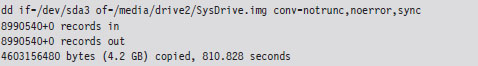
The problem with this approach is that it’s slow. Very, very, slow. The resulting disk image is a low-level reproduction that doesn’t distinguish between used and unused sectors. Everything on the original is simply copied over, block by block.
One solution that I’ve used for disk imaging is PING1 (Partimage Is Not Ghost). PING is basically a live Linux CD with built-in network support that relies on a set of open-source disk-cloning tools. The interface is friendly and fairly self-evident.
ASIDE
Regardless of which disk-imaging solution you choose, I would urge you to consider using a network setup where the client machine receives its image from a network server. Though this might sound like a lot of hassle, it can easily cut your imaging time in half. My own experience has shown that imaging over gigabit Ethernet can be faster than both optical media and external drives. This is one of those things that seems counterintuitive at the outset but proves to be a genuine time-saver.
For Faster Relief: Virtual Machines
If your system has the horsepower to support it, I’d strongly recommend running your development environment inside of a virtual machine that’s executing on top of a bare-metal hypervisor. The standard packages in this arena include VMWare’s ESXi and Microsoft’s Hyper-V. Given that I’ve chosen Windows 7 as a target platform, I prefer Hyper-V. Like I said, no one knows Windows like Microsoft.
Be warned that if you decide to go with Hyper-V, your system will need to be based on x64 hardware that has Intel VT or AMD-V technology enabled. In other words, you’ll be running a virtual 32-bit guest OS (Windows 7) on a hypervisor that’s using 64-bit physical processors.
Note: As mentioned in this book’s preface, we’re targeting the prototypical desktop machine that lies somewhere in a vast corporate cube farm. That means we’re assuming a commodity 32-bit processor running Windows 7. Using 64-bit hardware to support virtual machines doesn’t necessarily infer that our focus has changed. In other words, I’m not assuming that we’ll be attacking a 64-bit system that’s hosting a 32-bit Windows 7 guest operating system. Think of this more as a development crutch rather than an actual deployment scenario.
The advantage of using a virtual machine is speed. Restoring a virtual machine to its original state is typically much faster than the traditional reimaging process. Most bare-metal hypervisor-based environments allow you to create some sort of snapshot of a virtual machine, which represents the state of the virtual machine frozen in time. This way you can take a snapshot of your development environment, wreck it beyond repair, and then simply revert the virtual machine back to its original state when the snapshot was taken. This can be an incredible time-saver, resulting in a much shorter development cycle.
Finally, there’s a bit of marketing terminology being bandied about by the folks in Redmond that muddies the water. Windows Server 2008 R2 is a 64-bit operating system that can install Hyper-V as a server role. This gives you access to most of the bells and whistles (e.g., MMC snap-ins and the like) from within the standard Windows environment. Microsoft Hyper-V Server 2008 R2 is a free stand-alone product that offers a bare-bones instance of Hyper-V technology. The basic UI resembles that of the Server Core version of Windows. You get a command prompt, and that’s it. To make the distinction clear, I’m going to line up these terms next to each other:
 Windows Server 2008 R2.
Microsoft Hyper-V Server 2008 R2.
Notice how, with the stand-alone product, the term “Windows” is replaced by “Microsoft” and the word “Server” is placed after “Hyper-V.” This confused the hell out of me when I first started looking into this product. There are times when I wonder if this ambiguity was intentional?
Tool Roundup
For your edification, Table 5.1 summarizes the various tools that I’ve collected during my own foray into rootkits. All of them are free and can be downloaded off the Internet. I have no agenda here, just a desire to get the job done.
Table 5.1 Tool Roundup
| Tool | Purpose | Notable Features, Extras |
| Visual Studio Express | User-mode applications | Flexible IDE environment |
| Windows SDK | User-mode applications | Windows API docs, dumpbin.exe |
| WDK | Kernel-mode drivers | Windows debugging tools |
| Server 2003 DDK | Kernel-mode drivers | 16-bit real-mode tools |
| Sysinternals Suite | Diagnostic tools | The source code to NotMyFault. exe |
| Windows AIK | System cloning | ImageX.exe |
| Hyper-V Server 2008 R2 | Virtualization | Hyper-V integration services |
| Cygnus Hex Editor | Binary inspection/patching | Useful for shellcode extraction |
Though there may be crossover in terms of functionality, each kit tends to offer at least one feature that the others do not. For example, you can build user-mode apps with both the Windows SDK and Visual Studio Express. However, Visual Studio Express doesn’t ship with Windows API documentation.
5.2 Debuggers
When it comes to implementing a rootkit on Windows, debuggers are such essential tools that they deserve special attention. First and foremost, this is because you may need to troubleshoot a kernel-mode driver that’s misbehaving, and print statements can only take you so far. This doesn’t mean that you shouldn’t include tracing statements in your code; it’s just that sometimes they’re not enough. In the case of kernel-mode code (where the venerable printf() function is supplanted by DbgPrint()), debugging through print statements can be insufficient because certain types of errors result in system crashes, making it very difficult for the operating system to stream anything to the debugger’s console.
Another reason why debuggers are important is that they offer an additional degree of insight. Windows is a proprietary operating system. In the Windows Driver Kit, it’s fairly common to come across data structures and routines that are either partially documented or not documented at all. To see what I’m talking about, consider the declaration for the following kernel-mode routine:

The WDK online help states that this routine “returns a pointer to an opaque process object.”
That’s it, the EPROCESS object is opaque; Microsoft doesn’t say anything else. On a platform like Linux, you can at least read the source code. With Windows, to find out more you’ll need to crank up a kernel-mode debugger and sift through the contents of memory. We’ll do this several times over the next few chapters. The closed-source nature of Windows is one reason why taking the time to learn Intel assembly language and knowing how to use a debugger is a wise investment. The underlying tricks used to hide a rootkit come and go. But when push comes to shove, you can always disassemble to find a new technique. It’s not painless, but it works.
ASIDE
Microsoft does, in fact, give other organizations access to its source code; it’s just that the process occurs under tightly controlled circumstances. Specifically, I’m speaking of Microsoft’s Shared Source Initiative,2 which is a broad term referring to a number of programs where Microsoft allows original equipment manufacturers (OEMs), governments, and system integrators to view the source code to Windows. Individuals who qualify are issued smart cards and provided with online access to the source code via Microsoft’s Code Center Premium SSL-secured website. You’d be surprised who has access. For example, Microsoft has given access of its source code base to the Russian Federal Security Service (FSB).3
The first time I tried to set up two machines to perform kernel-mode debugging, I had a heck of a time. I couldn’t get the two computers to communicate, and the debugger constantly complained that my symbols were out of date. I nearly threw up my arms and quit (which is not an uncommon response). This brings us to the third reason why I’ve dedicated an entire section to debuggers: to spare readers the grief that I suffered through while getting a kernel-mode debugger to work.
The Debugging Tools for Windows package ships with four different debuggers:
The Microsoft Console Debugger (CDB.exe)
The NT Symbolic Debugger (NTSD.exe)
The Microsoft Kernel Debugger (KD.exe)
The Microsoft Windows Debugger (WinDbg.exe).
These tools can be classified in terms of the user interface they provide and the sort of programs they can debug (see Table 5.2). Both CDB.exe and NTSD.exe debug user-mode applications and are run from text-based command consoles. The only perceptible difference between the two debuggers is that NTSD.exe launches a new console window when it’s invoked. You can get the same behavior from CDB.exe by executing the following command:

The KD.exe debugger is the kernel-mode analogue to CDB.exe. The WinDbg.exe debugger is an all-purpose tool. It can do anything that the other debuggers can do, not to mention that it has a modest GUI that allows you to view several different aspects of a debugging session simultaneously.
Table 5.2 Debuggers
| Type of Debugger | User Mode | Kernel Mode |
| Console UI Debugger | CDB.exe, NTSD.exe | KD.exe |
| GUI Debugger | WinDbg.exe | WinDbg.exe |
In this section, I’m going to start with an abbreviated user’s guide for CDB.exe. This will serve as a lightweight warm-up for KD.exe and allow me to introduce a subset of basic debugger commands before taking the plunge into full-blown kernel debugging (which requires a bit more set up). After I’ve covered CDB.exe and KD.exe, you should be able to figure out WinDbg.exe on your own without much fanfare.
ASIDE
If you have access to source code and you’re debugging a user-mode application, you’d probably be better off using the integrated debugger that ships with Visual Studio. User-mode capable debuggers like CDB.exe or WinDbg.exe are more useful when you’re peeking at the internals of an unknown executable.
Configuring CDB.exe
Preparing to run CDB.exe involves two steps:
Establishing a debugging environment.
Acquiring the necessary symbol files.
The debugging environment consists of a handful of environmental variables. The three variables listed in Table 5.3 are particularly useful.
Table 5.3 CDB Environment
| Variable | Description |
| _NT_SOURCE_PATH | The path to the target binary’s source code files |
| _NT_SYMBOL_PATH | The path to the root node of the symbol file directory tree |
| _NT_DEBUG_LOG_FILE_OPEN | Specifies a log file used to record the debugging session |
The first two path variables can include multiple directories separated by semicolons. If you don’t have access to source code, you can simply neglect the _NT_SOURCE_PATH variable. The symbol path, however, is a necessity. If you specify a log file that already exists with the _NT_DEBUG_LOG_FILE_OPEN variable, the existing file will be overwritten.
Many environmental parameters specify information that can be fed to the debugger on the command line. This is a preferable approach if you wish to decouple the debugger from the shell that it runs under.
Symbol Files
Symbol files are used to store the programmatic metadata of an application. This metadata is archived according to a binary specification known as the Program Database Format. If the development tools are configured to generate symbol files, each executable/DLL/driver will have an associated symbol file with the same name as its binary and will be assigned the .pdb file extension. For instance, if I compiled a program named MyWinApp.exe, the symbol file would be named MyWinApp.pdb.
Symbol files contain two types of metadata:
Public symbol information.
Private symbol information.
Public symbol information includes the names and addresses of an application’s functions. It also includes a description of each global variable (i.e., name, address, and data type), compound data type, and class defined in the source code.
Private symbol information describes less visible program elements, like local variables, and facilitates the mapping of source code lines to machine instructions.
A full symbol file contains both public and private symbol information. A stripped symbol file contains only public symbol information. Raw binaries (in the absence of an accompanying .pdb file) will often have public symbol information embedded in them. These are known as exported symbols.
You can use the SymChk.exe command (which ships with the Debugging Tools for Windows) to see if a symbol file contains private symbol information:

The /r switch identifies the executable whose symbol file we want to check. The /s switch specifies the path to the directory containing the symbol file. The /ps option indicates that we want to determine if the symbol file has been stripped. In the case above, MyWinApp.pdb has not been stripped and still contains private symbol information.
Windows Symbols
Microsoft allows the public to download its OS symbol files for free. These files help you to follow the path of execution, with a debugger, when program control takes you into a Windows module. If you visit the website, you’ll see that these symbol files are listed by processor type (x86, Itanium, and x64) and by build type (Retail and Checked).
ASIDE
My own experience with Windows symbol packages was frustrating. I’d go to Microsoft’s website, spend a couple of hours downloading a 200-MB file, and then wait for another 30 minutes while the symbols installed … only to find out that the symbols were out of date (the Window’s kernel debugger complained about this a lot).
What I discovered is that relying on the official symbol packages is a lost cause. They constantly lag behind the onslaught of updates and hot fixes that Microsoft distributes via Windows Update. To stay current, you need to go directly to the source and point your debugger to Microsoft’s online symbol server. This way you’ll get the most recent symbol information.
According to Microsoft’s Knowledge Base Article 311503, you can use the online symbol server by setting the _NT_SYMBOL_PATH:
symsrv*symsrv.dll*<LocalPath>*http://msdl.microsoft.com/download/symbols
In the previous setting, the <LocalPath> string is a symbol path root on your local machine. I tend to use something like C:\windows\symbols or C:\symbols.
Retail symbols (also referred to as free symbols) are the symbols corresponding to the Free Build of Windows. The Free Build is the release of Windows compiled with full optimization. In the Free Build, debugging asserts (e.g., error checking and argument verification) have been disabled, and a certain amount of symbol information has been stripped away. Most people who buy Windows end up with the Free Build. Think retail, as in “Retail Store.”
Checked symbols are the symbols associated with the Checked Build of Windows. The Checked Build binaries are larger than those of the Free Build. In the Checked Build, optimization has been precluded in the interest of enabled debugging asserts. This version of Windows is used by people writing device drivers because it contains extra code and symbols that ease the development process.
Invoking CDB.exe
There are three ways in which CDB.exe can debug a user-mode application:
CDB.exe launches the application.
CDB.exe attaches itself to a process that’s already running.
CDB.exe targets a process for noninvasive debugging.
The method you choose will determine how you invoke CDB.exe on the command line. For example, to launch an application for debugging, you’d invoke CDB.exe as follows:

You can attach the debugger to a process that’s running using either the -p or -pn switch:

You can noninvasively examine a process that’s already running by adding the -pv switch:

Noninvasive debugging allows the debugger to “look without touching.” In other words, the state of the running process can be observed without affecting it. Specifically, the targeted process is frozen in a state of suspended animation, giving the debugger read-only access to its machine context (e.g., the contents of registers, memory, etc.).
As mentioned earlier, there are a number of command-line options that can be fed to CDB.exe as a substitute for setting up environmental variables:
-logo logFile used in place of _NT_DEBUG_LOG_FILE_OPEN
-y SymbolPath used in place of _NT_SYMBOL_PATH
-srcpath SourcePath used in place of _NT_SOURCE_PATH
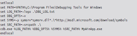
The following is a batch file template that can be used to invoke CDB.exe. It uses a combination of environmental variables and command-line options to launch an application for debugging:
Controlling CDB.exe
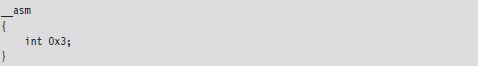
Debuggers use special instructions called break points to suspend temporarily the execution of the process under observation. One way to insert a break point into a program is at compile time with the following statement:
This tactic is awkward because inserting additional break points or deleting existing break points requires traversing the build cycle. It’s much easier to manage break points dynamically while the debugger is running. Table 5.4 lists a couple of frequently used commands for manipulating break points under CDB.exe.
Table 5.4 Break point Commands
| Command | Description |
| bl | Lists the existing break points (they’ll have numeric IDs) |
| bc breakpointID | Deletes the specified break point (using its numeric ID) |
| bp functionName | Sets a break point at the first byte of the specified routine |
| bp | Sets a break point at the location currently indicated by the IP register |
When CDB.exe launches an application for debugging, two break points are automatically inserted. The first suspends execution just after the application’s image (and its statically linked DLLs) has loaded. The second break point suspends execution just after the process being debugged terminates. The CDB.exe debugger can be configured to ignore these break points using the -g and -G command-line switches, respectively.
Once a break point has been reached, and you’ve had the chance to poke around a bit, the commands in Table 5.5 can be used to determine how the targeted process will resume execution. If the CDB.exe ever hangs or becomes unresponsive, you can always yank open the emergency escape hatch (e.g., “abruptly” exit the debugger) by pressing the CTRL+B key combination followed by the ENTER key.
Table 5.5 Execution Control
| Command | Description |
| g | (go) execute until the next break point |
| t | (trace) execute the next instruction (step into a function call) |
| p | (step) execute the next instruction (step over a function call) |
| gu | (go up) execute until the current function returns |
| q | (quit) exit CDB.exe and terminate the program being debugged |
Useful Debugger Commands
There are well over 200 distinct debugger commands, meta-commands, and extension commands. In the interest of brevity, what I’d like to do in this section is to present a handful of commands that are both relevant and practical in terms of the day-to-day needs of a rootkit developer. I’ll start by showing you how to enumerate available symbols. Next, I’ll demo a couple of ways to determine what sort of objects these symbols represent (e.g., data or code). Then I’ll illustrate how you can find out more about these symbols depending on whether a given symbol represents a data structure or a function.
Examine Symbols Command (x)
One of the first things that you’ll want to do after loading a new binary is to enumerate symbols of interest. This will give you a feel for the services that the debug target provides. The Examine Symbols command takes an argument of the form:
moduleName!Symbol
This specifies a particular symbol within a given module. You can use wild cards in both the module name and symbol name to refer to a range of possible symbols. Think of this command’s argument as a filtering mechanism. The Examine Symbols command lists all of the symbols that match the filter expression (see Table 5.6).
Table 5.6 Symbol Examination Commands
| Command | Description |
| x module!symbol | Report the address of the specified symbol (if it exists) |
| x *! | List all of the modules currently loaded |
| x module!* | List all of the symbols and their addresses in the specified module |
| x module!symbol* | List all of the symbols that match the “arg*” wild-card filter |
The following log file snippet shows this command in action.
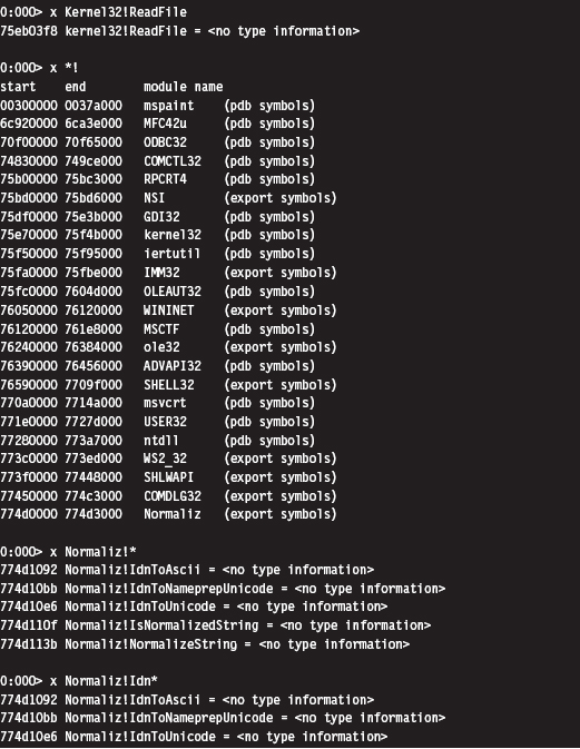
Looking at the previous output, you might notice that the symbols within a particular module are marked as indicating <no type information>. In other words, the debugger cannot tell you if the symbol is a function or a variable.
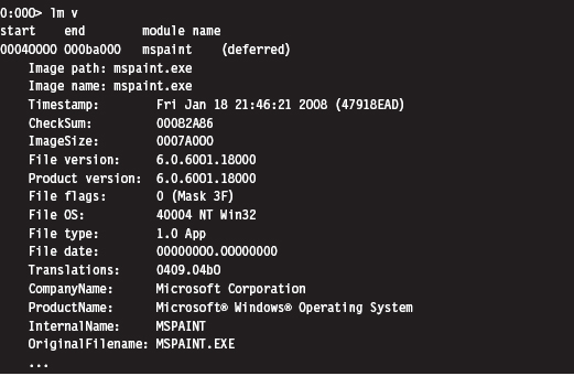
List Loaded Modules (1m and !1mi)
Previously you saw how the Examine Symbols command could be used to enumerate all of the currently loaded modules. The List Loaded Modules command offers similar functionality but with finer granularity of detail. The verbose option for this command, in particular, dumps out almost everything you’d ever want to know about a given binary.
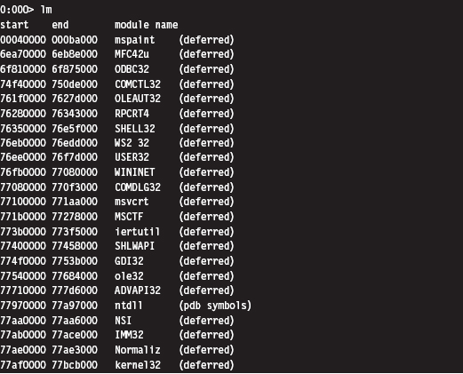
The !lmi extension command accepts that name, or base address, of a module as an argument and displays information about the module. Typically, you’ll run the lm command to enumerate the modules currently loaded and then run the !lmi command to find out more about a particular module.
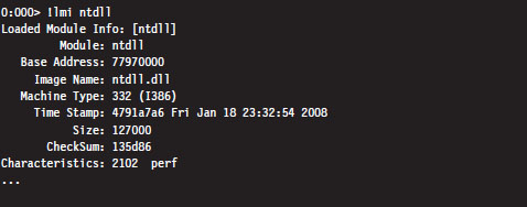
The verbose version of the List Loaded Modules command offers the same sort of extended information as !lmi.
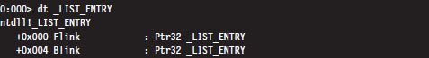
Display Type Command (dt)
Once you’ve identified a symbol, it would be useful to know what it represents. Is it a function or a variable? If a symbol represents data storage of some sort (e.g., a variable, a structure, or union), the Display Type command can be used to display metadata that describes this storage.
For example, we can see that the _LIST_ENTRY structure consists of two fields that are both pointers to other _LIST_ENTRY structures. In practice the _LIST_ENTRY structure is used to implement doubly linked lists, and you will see this data structure all over the place. It’s formally defined in the WDK’s ntdef.h header file.
Unassemble Command (u)
If a symbol represents a routine, this command will help you determine what it does. The unassemble command takes a specified region of memory and decodes it into Intel assembler and machine code. There are several different forms that this command can take (see Table 5.7).
Table 5.7 Disassembly Commands
| Command | Description |
| u | Disassemble 8 instructions starting at the current address |
| u address | Disassemble 8 instructions starting at the specified linear address |
| u start end | Disassemble memory residing in the specified address range |
| uf routineName | Disassemble the specified routine |
The first version, which is invoked without any arguments, disassembles memory starting at the current address (i.e., the current value in the EIP register) and continues onward for eight instructions (on the IA-32 platform). You can specify a starting linear address explicitly or an address range. The address can be a numeric literal or a symbol.
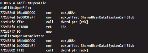
In the previous instance, the NtOpenFile routine consists of fewer than eight instructions. The debugger simply forges ahead, disassembling the code that follows the routine. The debugger indicates which routine this code belongs to (i.e., ZwOpenIoCompletion).
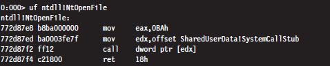
If you know that a symbol or a particular address represents the starting point of a function, you can use the Unassemble Function command (uf) to examine its implementation.
Display Commands (d*)
If a symbol represents data storage, this command will help you find out what’s being stored in memory. This command has many different incarnations (see Table 5.8). Most versions of this command take an address range as an argument. If an address range isn’t provided, a display command will typically dump memory starting where the last display command left off (or at the current value of the EIP register, if a previous display command hasn’t been issued) and continue for some default length.
Table 5.8 Data Display Commands
| Command | Description |
| db addressRange | Display byte values both in hex and ASCII (default count is 128) |
| dW addressRange | Display word values both in hex and ASCII (default count is 64) |
| dd addressRange | Display double-word values (default count is 32) |
| dps addressRange | Display and resolve a pointer table (default count is 128 bytes) |
| dg start End | Display the segment descriptors for the given range of selectors |
The following examples demonstrate different forms that the addressRange argument can take:
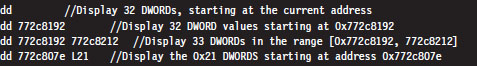
The last range format uses an initial address and an object count prefixed by the letter “L.” The size of the object in an object count depends upon the units of measure being used by the command. Note also how the object count is specified using hexadecimal.
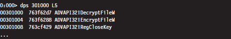
If you ever encounter a call table (a contiguous array of function pointers), you can resolve its addresses to the routines that they point to with the dps command. In the following example, this command is used to dump the import address table (IAT) of the advapi32.dll library in the mspaint.exe program. The IAT is a call table used to specify the address of the routines imported by an application. We’ll see the IAT again in the next chapter.
Note: The IA-32 platform adheres to a little-endian architecture. The least significant byte of a multi-byte value will always reside at the lowest address (Figure 5.1).
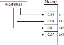
Figure 5.1
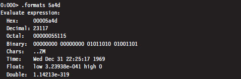
If you ever need to convert a value from hexadecimal to binary or decimal, you can use the Show Number Formats meta-command.
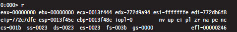
Registers Command (r)
This is the old faithful of debugger commands. Invoked by itself, it displays the general-purpose (i.e., non-floating-point) registers.
5.3 The KD.exe Kernel Debugger
Although the CDB.exe debugger has its place, its introduction was actually intended to prepare you for the main course: kernel debugging. Remember the initial discussion about symbol files and the dozen or so CDB.exe debugger commands we looked at? This wasn’t just wasted bandwidth. All of the material is equally valid in the workspace of the Windows kernel debugger (KD. exe). In other words, the Examine Symbols debugger command works pretty much the same way with KD.exe as it does with CDB.exe. My goal from here on out is to build upon the previous material, focusing on features related to the kernel debugger.
Different Ways to Use a Kernel Debugger
There are four different ways to use a kernel debugger to examine a system:
Using a physical host–target configuration.
Local kernel debugging.
Analyzing a crash dump.
Using a virtual host–target configuration.
One of the primary features of a kernel debugger is that it allows you to suspend and manipulate the state of the entire system (not just a single user-mode application). The caveat associated with this feature is that performing an interactive kernel-debugging session requires the debugger itself to reside on a separate machine.
If you think about it for a minute, this condition does make sense: If the debugger was running on the system being debugged, the minute you hit a break point the kernel debugger would be frozen along with the rest of the system, and you’d be stuck!
To control a system properly, you need a frame of reference that lies outside of the system being manipulated. In the typical kernel-debugging scenario, there’ll be a kernel debugger running on one computer (referred to as the host machine) that’s controlling the execution paths of another computer (called the target machine). These two machines will communicate over a serial cable or perhaps a special-purpose USB cable (Figure 5.2).
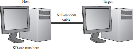
Figure 5.2
Despite the depth of insight that the host–target configuration yields, it can be inconvenient to have to set up two machines to see what’s going on. This leads us to the other three methods, all of which can be used with only a single physical machine.
Local kernel debugging is a hobbled form of kernel debugging that was introduced with Windows XP. Local kernel debugging is somewhat passive. Whereas it allows memory to be read and written to, there are a number of other fundamental operations that are disabled. For example, all of the kernel debugger’s break-point commands (set breakpoint, clear breakpoint, list breakpoints, etc.) and execution control commands (go, trace, step, step up, etc.) don’t function. In addition, register display commands and stack trace commands are also inoperative.
Microsoft’s documentation probably best summarizes the downside of local kernel debugging:
“One of the most difficult aspects of local kernel debugging is that the machine state is constantly changing. Memory is paged in and out, the active process constantly changes, and virtual address contexts do not remain constant. However, under these conditions, you can effectively analyze things that change slowly, such as certain device states.
Kernel-mode drivers and the Windows operating system frequently send messages to the kernel debugger by using DbgPrint and related functions. These messages are not automatically displayed during local kernel debugging.”
ASIDE
There’s a tool from Sysinternals called LiveKD.exe that emulates a local kernel debugging session by taking a moving snapshot (via a dump file) of the system’s state. Because the resulting dump file is created while the system is still running, the snapshot may represent an amalgam of several states.
In light of the inherent limitations, I won’t discuss local kernel debugging in this book. Target–host debugging affords a much higher degree of control and accuracy.
A crash dump is a snapshot of a machine’s state that persists as a binary file. Windows can be configured to create a crash dump file in the event of a bug check (also known as a stop error, system crash, or Blue Screen of Death; it’s a terminal error that kills the machine). A crash dump can also be generated on demand. The amount of information contained in a crash dump file can vary, depending upon how the process of creation occurs.
The KD.exe debugger can open a dump file and examine the state of the machine as if it were attached to a target machine. As with local kernel debugging, the caveat is that KD.exe doesn’t offer the same degree of versatility when working with crash dumps. Although using dump files is less complicated, you don’t have access to all of the commands that you normally would (e.g., break-point management and execution control commands). Nevertheless, researchers like Dmitry Vostokov have written multivolume anthologies on crash dump analysis. It is an entire area of investigation unto itself.
Finally, if you have the requisite horsepower, you can try to have your cake and eat it, too, by using a virtual host–target configuration. In this setup, the host machine and target machine are virtual machine partitions that communicate locally over a named pipe. With this arrangement, you get the flexibility of the two-machine approach on a single physical machine. Initially I eschewed this approach because the Windows technology stack in this arena was still new and not always stable. As Microsoft has refined its Hyper-V code base, I’ve become much more comfortable with this approach.
Physical Host–Target Configuration
Getting a physical host–target setup working can be a challenge. Both hardware and software components must be functioning properly. Getting two machines to participate in a kernel-debugging configuration is the gauntlet, so to speak. If you can get them running properly, everything else is downhill from there.
Preparing the Hardware
The target and host machines can be connected using one of the following types of cables:
Null-modem cable.
IEEE 1394 cable (Apple’s “Firewire,” or Sony’s “i.LINK”).
USB 2.0 debug cable.
Both USB 2.0 and IEEE 1394 are much faster options than the traditional null-modem, and this can mean something when you’re transferring a 3-GB core dump during a debug session. However, these newer options are also much more complicated to set up and can hit you in the wallet (the last time I checked, PLX Technologies manufactures a USB 2.0 debug cable that sells for $83).
Hence, I decided to stick with the least common denominator, a technology that has existed since the prehistoric days of the mainframe: the null-modem cable. Null-modem cables have been around so long that I felt pretty safe that they would work (if anything would). They’re cheap, readily available, and darn near every machine has a serial port.
A null-modem cable is just a run-of-the-mill RS-232 serial cable that has had its transmit and receive lines cross-linked so that one guy’s send is the other guy’s receive (and vice versa). It looks like any other serial cable with the exception that both ends are female (see Figure 5.3).
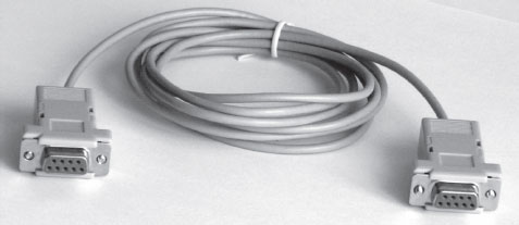
Figure 5.3
Before you link up your machines with a null-modem cable, you might want to reboot and check your BIOS to verify that your COM ports are enabled. You should also open up the Device Manager snap-in (devmgmt.msc) to ensure that Windows recognizes at least one COM port (see Figure 5.4).
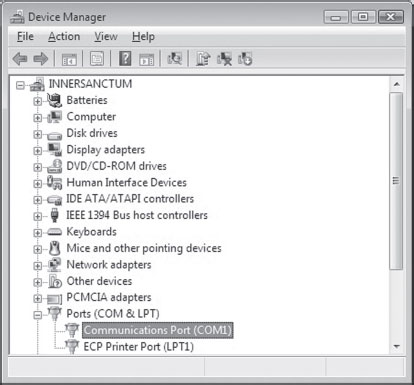
Figure 5.4
The Microsoft documents that come with the debugging tools want you to use HyperTerminal to check your null-modem connection. As an alternative to the officially sanctioned tool, I recommend using a free secure shell (SSH) client named PuTTY. PuTTY is a portable application; it requires no installation and has a small system footprint. Copy PuTTY.exe to both machines and double click it to initiate execution. You’ll be greeted by a Configuration screen that displays a category tree. Select the Session node and choose “Serial” for Connection type. PuTTY will auto-detect the first active COM port, populating the Serial line and Speed fields (see Figure 5.5).
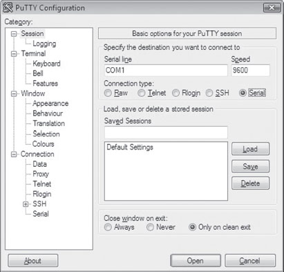
Figure 5.5
On both of my machines, these values defaulted to COM1 and 9600. Repeat this on the other machine and then press the Open button.
If fate smiles on you, this will launch a couple of Telnet-like consoles (one on each machine) where the characters you type on the keyboard of one computer end up on the console of the other computer. Don’t expect anything you type to be displayed on the machine that you’re typing on, look over at the other machine to see the output. This behavior will signal that your serial connection is alive and well.
Preparing the Software
Once you have the machines chatting over a serial line, you’ll need to make software-based adjustments. Given their distinct roles, each machine will have its own set of configuration adjustments.
On the target machine, you’ll need to tweak the boot configuration data file so that the boot manager can properly stage the boot process for kernel debugging. To this end, the following commands should be invoked on the target machine.

The first command enables kernel debugging during system bootstrap. The second command sets the global debugging parameters for the machine. Specifically, it causes the kernel debugging components on the target machine to use the COM1 serial port with a baud rate of 19,200 bps. The third command lists all of the settings in the boot configuration data file so that you can check your handiwork.
That’s it. That’s all you need to do on the target machine. Shut it down for the time being until the host machine is ready.
As with CDB.exe, preparing KD.exe for a debugging session on the host means:
Establishing a debugging environment.
Acquiring the necessary symbol files.
The debugging environment consists of a handful of environmental variables that can be set using a batch file. Table 5.9 provides a list of the more salient variables.
Table 5.9 Environmental Variables
| Variable | Description |
| _NT_DEBUG_PORT | The serial port used to communicate with the target machine |
| _NT_DEBUG_BAUD_RATE | The baud rate at which to communicate (in bps) |
| _NT_SYMBOL_PATH | The path to the root node of the symbol file directory tree |
| _NT_DEBUG_LOG_FILE_OPEN | Specifies a log file used to record the debugging session |
As before, it turns out that many of these environmental parameters specify information that can be fed to the debugger on the command line (which is the approach that I tend to take). This way you can invoke the debugger from any old command shell.
As I mentioned during my discussion of CDB.exe, with regard to symbol files I strongly recommend setting your host machine to use Microsoft’s symbol server (see Microsoft’s Knowledge Base Article 311503). Forget trying to use the downloadable symbol packages. If you’ve kept your target machine up to date with patches, the symbol file packages will almost always be out of date, and your kernel debugger will raise a stink about it.
I usually set the _NT_SYMBOL_PATH environmental variable to something like:
SRV*C:\mysymbols*http://msdl.microsoft.com/download/symbols
Launching a Kernel-Debugging Session
To initiate a kernel-debugging session, perform the following steps:
Turn the target system off.
Invoke the debugger (KD.exe) on the host.
Turn on the target system.
There are command-line options that can be fed to KD.exe as a substitute for setting up environmental variables (see Table 5.10).
Table 5.10 Command-Line Arguments
| Command-Line Argument | Corresponding Environmental Variable |
| -logo logFile | _NT_DEBUG_LOG_FILE_OPEN |
| -y SymbolPath | _NT_SYMBOL_PATH |
| -k com:port=n,baud=m | _NT_DEBUG_PORT, _NT_DEBUG_BAUD_RATE |
The following is a batch file template that can be used to invoke KD.exe. It uses a combination of environmental variables and command-line options to launch the kernel debugger:
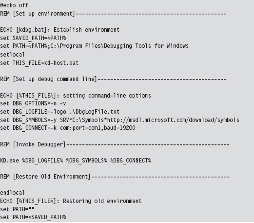
Once the batch file has been invoked, the host machine will sit and wait for the target machine to complete the connection.
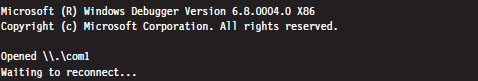
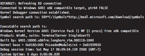
If everything works as it should, the debugging session will begin and you’ll see something like:

Controlling the Target
When the target machine has completed system startup, the kernel debugger will passively wait for you to do something. At this point, most people issue a break-point command by pressing the CTRL+C command keys on the host. This will suspend execution of the target computer and activate the kernel debugger, causing it to display a command prompt.
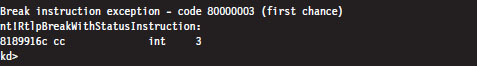
As you can see, our old friend the break-point interrupt hasn’t changed much since real mode. If you’d prefer that the kernel debugger automatically execute this initial break point, you should invoke KD.exe with the additional -b command-line switch.
The CTRL+C command keys can be used to cancel a debugger command once the debugger has become active. For example, let’s say that you’ve mistakenly issued a command that’s streaming a long list of output to the screen, and you don’t feel like waiting for the command to terminate before you move on. The CTRL+C command keys can be used to halt the command and give you back a kernel debugger prompt.
After you’ve hit a break point, you can control execution using the same set of commands that you used with CDB.exe (e.g., go, trace, step, go up, and quit). The one command where things get a little tricky is the quit command (q). If you execute the quit command from the host machine, the kernel debugger will exit leaving the target machine frozen, just like Sleeping Beauty. To quit the kernel debugger without freezing the target, execute the following three commands:

The first command clears all existing break points. The second command thaws out the target from its frozen state and allows it to continue executing. The third command-key sequence detaches the kernel debugger from the target and terminates the kernel debugger.
There are a couple of other command-key combinations worth mentioning. For example, if you press CTRL+V and then press the ENTER key, you can toggle the debugger’s verbose mode on and off. Also, if the target computer somehow becomes unresponsive, you can resynchronize it with the host machine by pressing the CTRL+R command keys followed by the ENTER key.
Virtual Host–Target Configuration
The traditional host–target setup, where you literally have two physical machines talking to each other over a wire, can be awkward and space-intensive, just like those old 21-inch CRTs that took up half of your desk space. If you’re using Hyper-V, you can save yourself a lot of grief by configuring the parent partition to act as the host and a child partition to act as the target.
You may be scratching your head right about now: What the heck is a partition?
Hyper-V refers to the operating systems running on top of the hypervisor as partitions. The parent partition is special in that it is the only partition that has access to the native drivers (e.g., the drivers that manage direct access to the physical hardware), and it is also the only partition that can use a management snap-in (virtmgmt.msc) to communicate with the hypervisor, such that the parent partition can create and manipulate other partitions.
The remaining partitions, the child partitions, are strictly virtual machines that can only access virtual hardware (see Figure 5.6). They don’t have the system-wide vantage point that the parent partition possesses. The child partitions are strictly oblivious citizens of the matrix. They don’t realize that they’re just software-based constructs sharing resources with other virtual machines on 64-bit hardware.
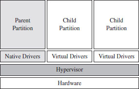
Figure 5.6
Configuring the parent partition to debug a child partition via KD.exe is remarkably simple. First, you install the Windows debugging tools on the parent partition. The debugging tools ship as an optional component of the Windows Driver Kit. Next, crank up the Hyper-V manager via the following command:

Right click the virtual machine you wish to debug and select the Settings menu. This will bring up the Settings window for the virtual machine. Select the COM1 item under the Hardware list and set it to use a named pipe (see Figure 5.7).
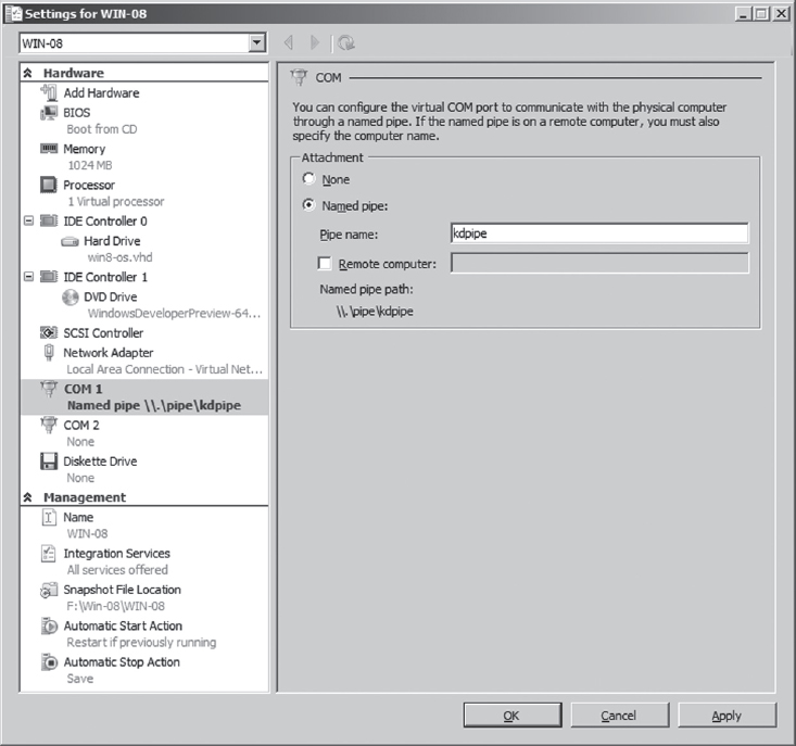
Figure 5.7
The name that you use is arbitrary. I use \\.\pipe\kdpipe. What’s important is that you need to modify the startup script that I provided earlier to invoke KD.exe in the case of two physical machines. We’re not using a serial cable anymore; we’re using a named pipe. Naturally, the connection parameters have to change. Specifically, you’ll need to take the line

and change it to

This completes the necessary configuration for the parent partition. On the child partition, you’ll need to enable kernel debugging via the following command:

That’s it. Now you can launch a kernel-debugging session just as you would for a physical host–target setup: turn the target system off, invoke the debugger (KD.exe) on the host, and then start the target system.
Useful Kernel-Mode Debugger Commands
All of the commands that we reviewed when we were looking at CDB.exe are also valid under KD.exe. Some of them have additional features that can be accessed in kernel mode. There is also a set of commands that are specific to KD.exe that cannot be utilized by CDB.exe. In this section, I’ll present some of the more notable examples.
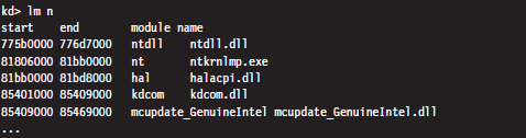
List Loaded Modules Command (lm)
In kernel mode, the List Loaded Modules command replaces the now-obsolete !drivers extension command as the preferred way to enumerate all of the currently loaded drivers.
!process
The !process extension command displays metadata corresponding to a particular process or to all processes. As you’ll see, this leads very naturally to other related kernel-mode extension commands.
The !process command assumes the following form:
!process Process Flags
The Process argument is either the process ID or the base address of the EPROCESS structure corresponding to the process. The Flags argument is a 5-bit value that dictates the level of detail that’s displayed. If Flags is zero, only a minimal amount of information is displayed. If Flags is 31, the maximum amount of information is displayed.
Most of the time, someone using this command will not know the process ID or base address of the process they’re interested in. To determine these values, you can specify zero for both arguments to the !process command, which will yield a bare-bones listing that describes all of the processes currently running.
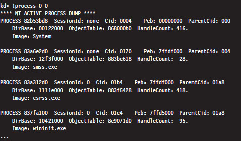
Let’s look at the second entry in particular, which describes smss.exe.
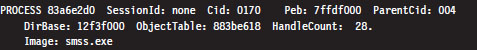
The numeric field following the word PROCESS (i.e., 83a6e2d0 ) is the base linear address of the EPROCESS structure associated with this instance of smss. exe. The Cid field (which has the value 0170) is the process ID. This provides us with the information we need to get a more in-depth look at some specific process (like calc.exe, for instance).
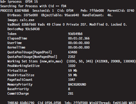
Every running process is represented by an executive process block (an EPROCESS block). The EPROCESS is a heavily nested construct that has dozens of fields storing all sorts of metadata on a process. It also includes substructures and pointers to other block structures. For example, the PEB field of the EPROCESS block points to the process environment block (PEB), which contains information about the process image, the DLLs that it imports, and the environmental variables that it recognizes.
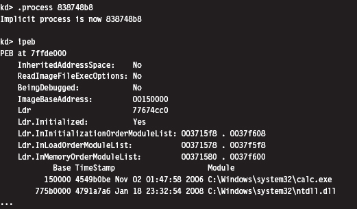
To dump the PEB, you set the current process context using the .process extension command (which accepts the base address of the EPROCESS block as an argument) and then issue the !peb extension command.
Registers Command (r)
In the context of a kernel debugger, the Registers command allows us to inspect the system registers. To display the system registers, issue the Registers command with the mask option (M) and an 8-bit mask flag. In the event that a computer has more than one processor, the processor ID prefixes the command. Processors are identified numerically, starting at zero.
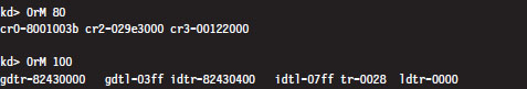
In the previous output, the first command uses the 0x80 mask to dump the control registers for the first processor (i.e., processor 0). The second command uses the 0x100 mask to dump the descriptor registers.
Working with Crash Dumps
Crash dump facilities were originally designed with the intent of allowing software engineers to analyze a system’s state, postmortem, in the event of a bug check. For people like you and me who dabble in rootkits, crash dump files are another reverse-engineering tool. Specifically, it’s a way to peek at kernel internals without requiring a two-machine setup.
There are three types of crash dump files:
Complete memory dump.
Kernel memory dump.
Small memory dump.
A complete memory dump is the largest of the three and includes the entire content of the system’s physical memory at the time of the event that led to the file’s creation. The kernel memory dump is smaller. It consists primarily of memory allocated to kernel-mode modules (e.g., a kernel memory dump doesn’t include memory allocated to user-mode applications). The small memory dump is the smallest of the three. It’s a 64-KB file that archives a bare-minimum amount of system metadata.
Because the complete memory dump offers the most accurate depiction of a system’s state, and because sub-terabyte hard drives are now fairly common, I recommend working with complete memory dump files. Terabyte external drives are the norm in this day and age. A 2- to 4-GB crash dump should pose little challenge.
There are three different ways to manually initiate the creation of a dump file:
Method no. 1: PS/2 keyboard trick.
Method no. 2: KD.exe command.
Method no. 3: NotMyFault.exe.
Method No. 1: PS/2 Keyboard Trick
The first thing you need to do is to open up the Control Panel and enable dump file creation. Launch the Control Panel’s System applet and select the Advanced System Settings option. Press the Settings button in the Startup and Recovery section to display the Startup and Recovery window (see Figure 5.8).
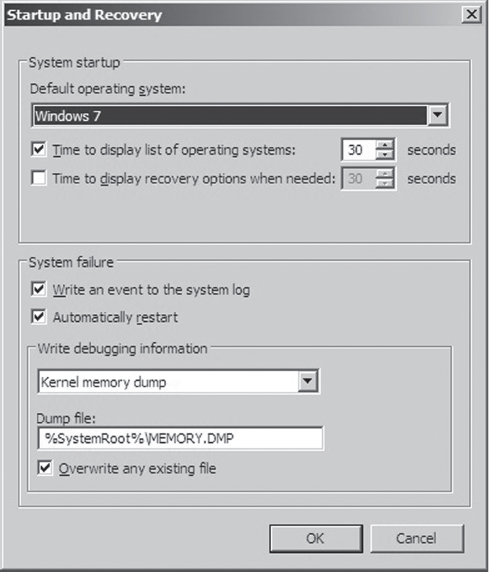
Figure 5.8
The fields in the lower portion of the screen will allow you to configure the type of dump file you wish to create and its location. Once you’ve enabled dump file creation, crank up Regedit.exe and open the following key:
HKLM\System\CurrentControlSet\Services\i8042prt\Parameters\
Under this key, create a DWORD value named CrashOnCtrlScroll and set it to 0x1. Then reboot your machine.
Note: This technique only works with non-USB keyboards!
After rebooting, you can manually initiate a bug check and generate a crash dump file by holding down the rightmost CTRL key while pressing the SCROLL LOCK key twice. This will precipitate a MANUALLY_INITIATED_CRASH bug check with a stop code of 0x000000E2. The stop code is simply a hexadecimal value that shows up on the Blue Screen of Death directly after the word “STOP.” For example, when a BSOD occurs as a result of an improper interrupt request line (IRQL), you may see something like:
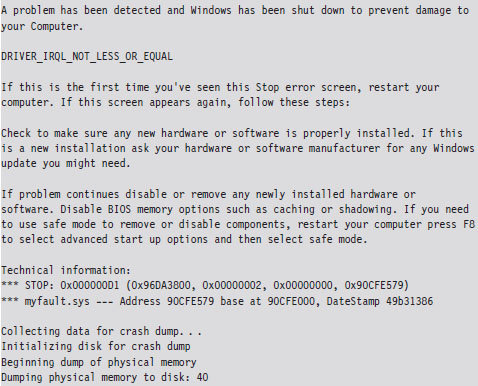
In this case, the stop code (also known as bug check code) is 0x000000D1, indicating that a kernel-mode driver attempted to access pageable memory at a process IRQL that was too high.
Method No. 2: KD.exe Command
This technique requires a two-machine setup. However, once the dump file has been generated, you only need a single computer to load and analyze the crash dump. As before, you should begin by enabling crash dump files via the Control Panel on the target machine. Next, you should begin a kernel-debugging session and invoke the following command from the host:

This will precipitate a MANUALLY_INITIATED_CRASH bug check with a stop code of 0x000000E2. The dump file will reside on the target machine. You can either copy it over to the host, as you would any other file, or install the Windows debugging tools on the target machine and run an analysis of the dump file there.
Method No. 3: NotMyFault.exe
This method is my personal favorite because it’s easy to do, and the tool is distributed with source code.4 The tool comes in two parts. The first part is an executable named NotMyFault.exe. This executable is a user-mode program that, at runtime, loads a kernel-mode driver, aptly named MyFault.sys, into memory.
The executable is the software equivalent of a front man that gets the kernel-mode driver to do its dirty work for it. Hence the naming scheme (one binary generates the actual bug check, and the other merely instigates it). The user-mode code, NotMyFault.exe, sports a modest GUI (see Figure 5.9) and is polite enough to allow you to pick your poison, so to speak. Once you press the “Do Bug” button, the system will come to a screeching halt, present you with a bug check, and leave a crash dump file in its wake.
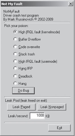
Figure 5.9
Crash Dump Analysis
Given a crash dump, you can load it using KD.exe in conjunction with the -z command-line option. You could easily modify the batch file I presented earlier in the chapter to this end.

After the dump file has been loaded, you can use the .bugcheck extension command to verify the origins of the crash dump.

Although using crash dump files to examine system internals may be more convenient than the host–target setup because you only need a single machine, there are trade-offs. The most obvious one is that a crash dump is a static snapshot, and this precludes the use of interactive commands that place break points or manage the flow of program control (e.g., go, trace, step, etc.).
If you’re not sure if a given command can be used during the analysis of a crash dump, the Windows debugging tools online help documentation specifies whether a command is limited to live debugging or not. For each command, reference the Target field under the command’s Environment section (see Figure 5.10).
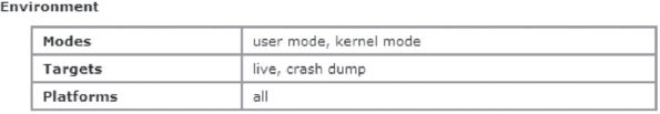
Figure 5.10
1. http://ping.windowsdream.com/.
2. http://www.microsoft.com/resources/sharedsource/default.mspx.
3. Tom Espiner, “Microsoft opens source code to Russian secret service,” ZDNet UK, July 8, 2010.