Table of Contents for

The Rootkit Arsenal: Escape and Evasion in the Dark Corners of the System, 2nd Edition

Chapter 7    Defeating Disk Analysis

---

 

As mentioned in this book’s preface, I’ve decided to present anti-forensics (AF) tactics in a manner that follows the evolution of the arms race itself. In the old days, computer forensics focused heavily (if not exclusively) on disk analysis. Typically, some guy in a suit would arrive on the scene with a briefcase-sized contraption to image the compromised machine, and that would be it. Hence, I’m going to start by looking at how this process can be undermined.

Given our emphasis on rootkit technology, I’ll be very careful to distinguish between low-and-slow tactics and scorched earth AF. Later on in the book, we’ll delve into live incident response and network security monitoring, which (in my opinion) is where the battlefront is headed over the long run.

7.1    Postmortem Investigation: An Overview

---

To provide you with a frame of reference, let’s run through the basic dance steps that constitute a postmortem examination. We’ll assume that the investigator has decided that it’s feasible to power down the machine in question and perform an autopsy. As described in Chapter 2, there are a number of paths that lead to a postmortem, and each one has its own set of trade-offs and peculiarities. Specifically, the investigator has the option to:

  Boldly yank the power cable outright.

  Perform a normal system shutdown.

  Initiate a kernel crash dump.

Regardless of how the dearly departed machine ended up comatose, the basic input to this multistage decomposition is either a disk image file or a physical duplicate copy that represents a sector-by-sector facsimile of the original storage medium. The investigator hopes to take this copy and, through an elaborate series of procedures, distill it into a set of unknown binaries (see Figure 7.1).

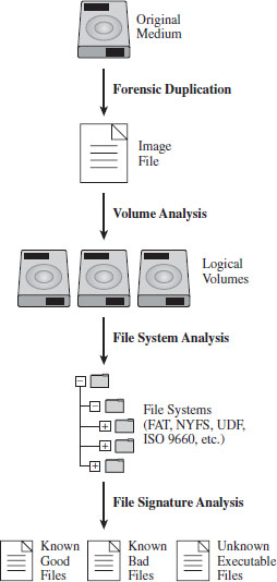
Figure 7.1

The AF researcher known as The Grugq has likened these various steps to the process of digestion in the multicompartment stomach of a cow (see Figure 7.2). This is novel enough that it will probably help you remember what’s going on. The forensic duplicate goes in at one end, gets partially digested, regurgitated back up, chewed up some more, digested yet again, and then expelled as a steaming pile of, … well, unknown executables.

In this chapter, I’ll focus strictly on the steps that lead us to the set of unknown executables and countermeasures that can be used by a rootkit. Analyzing an unknown executable is such a complicated ordeal that I’m going to defer immediate treatment and instead devote the entire next chapter to the topic.

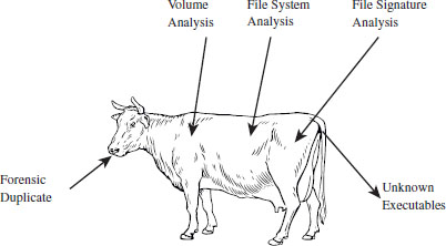
Figure 7.2

7.2    Forensic Duplication

---

In the interest of preserving the integrity of the original system, the investigator will begin by making a forensic duplicate of the machine’s secondary storage. As described in Chapter 2, this initial forensic duplicate will be used to spawn second-generation duplicates that can be examined and dissected at will. Forensic duplicates come in two flavors:

  Duplicate copies.

  Image files.

A duplicate copy is a physical disk that has been zeroed out before receiving data from the original physical drive. Sector 0 of the original disk is copied to sector 0 of the duplicate copy, and so on. This is an old-school approach that has been largely abandoned because you have to worry about things like disk geometry getting in the way. In this day and age, most investigators opt to store the bytes of the original storage medium as a large binary file, or image file.

Regardless of which approach is brought into play, the end goal is the same in either case: to produce an exact sector-by-sector replica that possesses all of the binary data, slack space, free space, and environmental data of the original storage.

In the spirit of Locard’s exchange principle, it’s a good idea to use a write blocker when creating or copying a forensic duplicate. A write blocker is a special-purpose hardware device or software application that protects drives from being altered, which is to say that they enforce a look-but-don’t-touch policy. Most investigators prefer the convenience of a hardware-based device. For example, the pocket-sized Tableau T35es shown in Figure 7.3 is a popular write blocker, often referred to as a forensic bridge, which supports imaging of IDE and SATA drives.

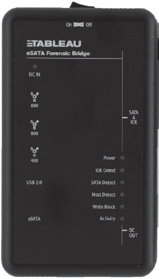
Figure 7.3

There are various well-known commercial tools that can be used to create a forensic duplicate of a hard drive, such as EnCase Forensic Edition from Guidance Software¹ or the Forensic Toolkit from Access Data.²

Forensic investigators on a budget (including your author) can always opt for freeware like the dcfldd package, which is a variant of dd written by Nick Harbour while he worked at the U.S. Department of Defense Computer Forensics Lab.³

Access Data also provides a tool called the FTK Imager for free. There’s even a low-impact version of it that doesn’t require installation.⁴ This comes in handy if you want to stick the tool on a CD or thumb drive. To use this tool, all you have to do is double click the FTK Imager.exe application, then click on the File Menu and select the Create Disk Image menu item (see Figure 7.4).

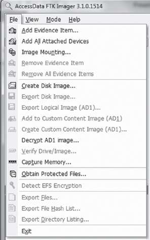
Figure 7.4 AccessData, Forensic Toolkit, Password Recovery Toolkit, PRTK, Distributed Network Attack and DNA are registered trademarks owned by AccessData in the United States and other jurisdictions and are used herein with permission from AccessData Group.

Then, you select the type of source that you want to image (e.g., a physical drive) and press the Next button (see Figure 7.5). Make sure that you have a write blocker hooked up to the drive you’ve chosen.

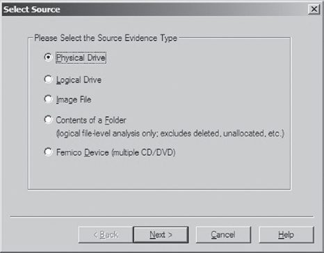
Figure 7.5

What follows is a fairly self-explanatory series of dialogue windows. You’ll be asked to select a physical drive, a destination to store the image file, and an image file format (e.g., I used the Raw (dd) format, which is practically an industry standard).

Countermeasures: Reserved Disk Regions

When it comes to foiling the process of forensic duplication, one way to beat the White Hats is to stash your files in a place that’s so far off the beaten track that they don’t end up as a part of the disk image.

Several years ago, the hiding spots of choice were the host protected area (HPA) and the device configuration overlay (DCO). The HPA is a reserved region on a hard drive that’s normally invisible to both the BIOS and host operating system. It was first established in the ATA-4 standard as a way to stow things like diagnostic tools and backup boot sectors. Some original equipment manufacturers (OEMs) have also used the HPA to store a disk image so that they don’t have to ship their machines with a re-install CD. The HPA of a hard drive is accessed and managed via a series of low-level ATA hardware commands.

Like the HPA, the DCO is also a reserved region on a hard drive that’s created and maintained through hardware-level ATA commands. DCOs allow a user to purchase drives from different vendors, which may vary slightly in terms of the amount of storage space that they offer, and then standardize them so that they all offer the same number of sectors. This usually leaves an unused area of disk space.

Any hard drive that complies with the ATA-6 standard can support both HPAs and DCOs, offering attackers a nifty way to stow their attack tools (assuming they know the proper ATA incantations). Once more, because these reserved areas aren’t normally recognized by the BIOS or the OS, they could be over-looked during the disk duplication phase of forensic investigation. The tools would fail to “see” the HPA or DCO and not include them in the disk image. For a while, attackers found a place that sheltered the brave and confounded the weak.

The bad news is that it didn’t take long for the commercial software vendors to catch on. Most commercial products worth their salt (like Tableau’s TD1 forensic duplicator) will detect and reveal these areas without much fanfare. In other words, if it’s on the disk somewhere, you can safely assume that the investigator will find it. Thus, reserved disk areas like the HPA or the DCO could be likened to medieval catapults; they’re historical artifacts of the arms race between attackers and defenders. If you’re dealing with a skilled forensic investigator, hiding raw, un-encoded data in the HPA or DCO offers little or no protection (or, even worse, a false sense of security).

7.3    Volume Analysis

---

With a disk image in hand, an investigator will seek to break it into volumes (logical drives) where each volume hosts a file system. In a sense, then, volume analysis can be seen as a brief intermediary phase, a staging process for file system analysis, which represents the bulk of the work to be done. We’ll get into file system analysis in the next section. For now, it’s worthwhile to examine the finer points of volume analysis under Windows. As you’ll see, it’s mostly a matter of understanding vernacular.

Storage Volumes under Windows

A partition is a consecutive group of sectors on a physical disk. A volume, in contrast, is a set of sectors (not necessarily consecutive) that can be used for storage. Thus, every partition is also a volume but not vice versa.

The tricky thing about a volume on the Windows platform is that the exact nature of a volume depends upon how Windows treats the underlying physical disk storage. As it turns out, Windows 7 running on 32-bit hardware supports two types of disk configurations:

  Basic disks.

  Dynamic disks.

A basic disk can consist of four partitions (known as primary partitions) where each partition is formatted with its own file system. Alternatively, a basic disk can house three primary partitions and a single extended partition, where the extended partition can support up to 128 logical drives (see Figure 7.6). In this scenario, each primary partition and logical drive hosts its own file system and is known as a basic volume. Basic disks like this are what you’re most likely to find on a desktop system.

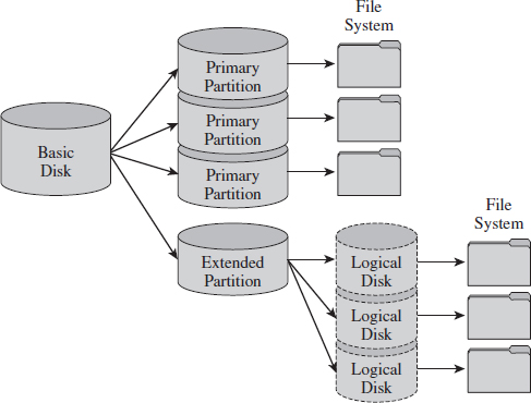
Figure 7.6

A dynamic disk can store up to 2,000 dynamic volumes. A dynamic volume can be created using a single region on a single dynamic disk or several regions on a single dynamic disk that have been linked together. In both of these cases, the dynamic volume is referred to as a simple volume. You can also merge several dynamic disks into a single dynamic volume (see Figure 7.7), which can then be formatted with a file system. If data is split up and spread out over the dynamic disks, the resulting dynamic volume is known as a striped volume. If data on one dynamic disk is duplicated to another dynamic disk, the resulting dynamic volume is known as a mirrored volume. If storage requirements are great enough that the data on one dynamic disk is expected to spill over into other dynamic disks, the resulting dynamic volume is known as a spanned volume.

So, there you have it. There are five types of volumes: basic, simple, striped, mirrored, and spanned. They all have one thing in common: each one hosts a single file system.

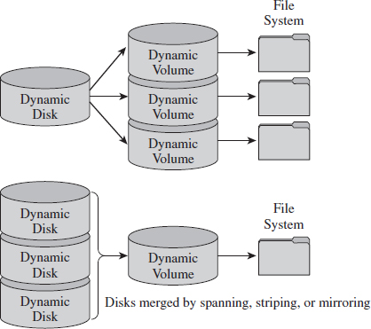
Figure 7.7

At this point, I feel obligated to insert a brief reality check. While dynamic volumes offer a lot of bells and whistles, systems that do use data striping or mirroring tend to do so at the hardware level. Can you imagine how abysmally slow software-based redundant array of independent disks (RAID-5) is? Good grief. Not to mention that this book is focusing on the desktop as a target, and most desktop systems still rely on basic disks that are partitioned using the MBR approach.

Manual Volume Analysis

Commercial tools will split a disk image into volumes automatically. But if you want to explicitly examine the partition table of a basic disk, you can use the mmls tool that ships with Brian Carrier’s Sleuth Kit.⁵

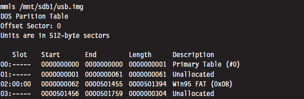
The first column is just a sequential counter that has no correlation to the physical partition table. The second column (e.g., the slot column) indicates which partition table a given partition belongs to and its relative location in that partition table. For example, a slot value of 01:02 would specify entry 02 in partition table 01.

If you prefer a GUI tool, Symantec still offers the PowerQuest Partition Table Editor at its FTP site.⁶ Keep in mind that you’ll need to run this tool with administrative privileges. Otherwise it will balk and refuse to launch.

Figure 7.8 displays the partition table for a Dell desktop system. This is evident because the first partition is a DELL OEM partition (Type set to 0×DE). The next two partitions are formatted by NTFS file systems (Type set to 0×07). The second partition, directly after the OEM partition, is the system volume that the OS will boot from (e.g., its Boot column is set to “active,” or 0×80). This is a fairly pedestrian setup for a desktop machine. You’ve got a small OEM partition used to stash diagnostic utilities, a combined system volume and boot volume, in addition to a third partition that’s most likely intended to store data. This way, if the operating system takes a nosedive, the help-desk technicians can re-install the OS and perhaps still salvage the user’s files.

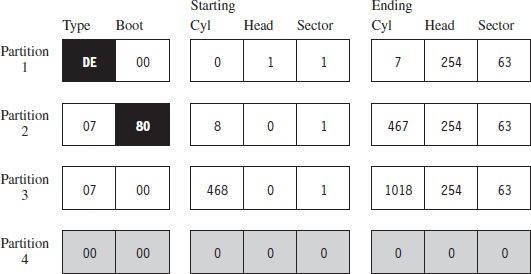
Figure 7.8

Countermeasures: Partition Table Destruction

One way to hinder the process of volume analysis is to vandalize the partition table. Granted, this is a scorched earth strategy that will indicate that something is amiss. In other words, this is not an AF approach that a rootkit should use. It’s more like a weapon of last resort that you could use if you suspect that you’ve already been detected and you want to buy a little time.

Another problem with this strategy is that there are tools like Michail Brzitwa’s gpart⁷ and Chris Grenier’s TestDisk⁸ that can recover partition tables that have been corrupted. Applications like gpart work by scanning a disk image for patterns that mark the beginning of a specific file system. This heuristic technique facilitates the re-creation of a tentative partition table (which may, or may not, be accurate).

Obviously, there’s nothing to stop you from populating the targeted disk with a series of byte streams that appear to denote the beginning of a file system. The more false positives you inject, the more time you force the investigator to waste.

A truly paranoid system administrator may very well back up his or her partition tables as a contingency. This is easier than you think. All it takes is a command like:

Thus, if you’re going to walk down the scorched earth path, you might as well lay waste to the entire disk and undermine its associated file system data structures in addition to the partition table. This will entail raw access to disk storage.

Raw Disk Access under Windows

At the Syscan’06 conference in Singapore, Joanna Rutkowska demonstrated how to inject code into kernel space, effectively side-stepping the driver signing requirements instituted on the 64-bit version of Vista. The basic game plan of this hack involved allocating a lot of memory (via the VirtualAllocEx() system call) to encourage Windows to swap out a pageable driver code section to disk. Once the driver code was paged out to disk, it was overwritten with arbitrary shellcode that would be invoked once the driver was loaded back into memory.

Driver sections that are pageable have names that start with the string “PAGE.” You can verify this using dumpbin.exe.

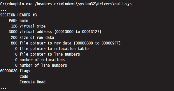
Rutkowska began by looking for some obscure KMD that contained pageable code sections. She settled on the null.sys driver that ships with Windows. It just so happens that the IRP dispatch routine exists inside of the driver’s pageable section (you can check this yourself with IDA Pro). Rutkowska developed a set of heuristics to determine how much memory would need to be allocated to force the relevant portion of null.sys to disk.

Once the driver’s section was written to disk, its dispatch routine was located by a brute-force scan of the page file that searched for a specific multi-byte pattern. Reading the Windows page file and implementing the corresponding shellcode patch was facilitated by CreateFile(“\\\\.\\PhysicalDisk0”,… ), which offers user-mode programs raw access to disk sectors. To coax the operating system to load and run the shellcode, CreateFile() can be invoked to open the driver’s object and get the Windows I/O manager to fire off an IRP.

In her original presentation, Rutkowska examined three ways to defend against this attack:

  Disable paging (who needs paging when 4 GB of RAM is affordable?).

  Encrypt or signature pages swapped to disk (performance may suffer).

  Disable user-mode access to raw disk sectors (the easy way out).

Microsoft has since addressed this attack by hobbling user-mode access to raw disk sectors on Vista. Now, I can’t say with 100% certainty that Joanna’s nifty hack was the precipitating incident that led Microsoft to institute this policy, but I wouldn’t be surprised.

Note that this does nothing to prevent raw disk access in kernel mode. Rutkowska responded⁹ to Microsoft’s solution by noting that all it would take to surmount this obstacle is for some legitimate software vendor to come out with a disk editor that accesses raw sectors using its own signed KMD. An attacker could then leverage this signed driver, which is 100% legitimate, and commandeer its functionality to inject code into kernel space using the attack just described!

Rutkowska’s preferred defense is simply to disable paging and be done with it.

Raw Disk Access: Exceptions to the Rule

If you’re going to lay waste to a drive in an effort to stymie a postmortem, it would probably be a good idea to read the fine print with regard to the restrictions imposed on user-mode access to disk storage (see Microsoft Knowledge Base Article 942448¹⁰).

Notice how the aforementioned article stipulates that boot sector access is still allowed “to support programs such as antivirus programs, setup programs, and other programs that have to update the startup code of the system volume.” Ahem. The details of raw disk access on Windows have been spelled out in Knowledge Base Article 100027.¹¹ There are also fairly solid operational details given in the MSDN documentation of the CreateFile() and WriteFile() Windows API calls.

Another exception to the rule has been established for accessing disk sectors that lie outside of a file system. Taken together with the exception for manipulating the MBR, you have everything you need to implement a bootkit (we’ll look into these later on in the book). For the time being, simply remember that sabotaging the file system is probably best done from the confines of kernel mode.

Nevertheless, altering a disk’s MBR from user mode is pretty straightforward if that’s what you want to do. The code snippet that follows demonstrates how this is done.

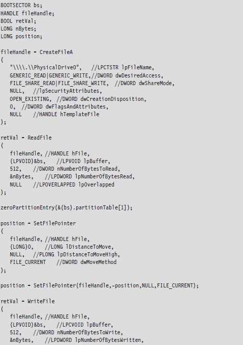
This code starts by opening up a physical drive and reading the MBR into a structure of type BOOTSECTOR:

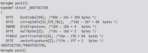
Notice how I used a #pragma directive to control byte alignment. In a 512-byte MBR, bytes 0×1BE through 0×1FD are consumed by the partition table, which in this case is represented by an array of four partition table structures (we’ll dive into the deep end later on in the book when we examine bootkits). For now, you just need to get a general idea of what’s going on.

Once I’ve read in the MBR, I’m in a position where I can selectively alter entries and then write them back to disk. Because I’m writing in addition to reading, this code needs to query the file pointer’s position via special parameters to SetFilePointer() and then rewind back to the start of the byte stream with a second call to SetFilePointer(). If you try to write beyond the MBR and into the inner reaches of the file system, the WriteFile() routine will balk and give you an error message. This is the operating system doing its job in kernel mode on the other side of the great divide.

7.4    File System Analysis

---

Once an investigator has enumerated the volumes contained in his forensic duplicate, he can begin analyzing the file systems that those volumes host. His general goal will be to maximize his initial data set by extracting as many files, and fragments of files, that he can. A file system may be likened to a sponge, and the forensic investigator wants to squeeze as much as he can out of it. Statistically speaking, this will increase his odds of identifying an intruder.

To this end, the investigator will attempt to recover deleted files, look for files concealed in alternate data streams (ADSs), and check for useful data in slack space. Once he’s got his initial set of files, he’ll harvest the metadata associated with each file (i.e., full path, size, time stamps, hash checksums, etc.) with the aim of creating a snapshot of the file system’s state.

In the best-case scenario, an initial baseline snapshot of the system has already been archived, and it can be used as a point of reference for comparison. We’ll assume that this is the case in an effort to give our opposition the benefit of the doubt.

The forensic investigator can then use these two snapshots (the initial baseline snapshot and the current snapshot) to whittle away at his list of files, removing files that exist in the original snapshot and don’t show signs of being altered. Concurrently, he can also identify files that demonstrate overt signs of being malicious. In other words, he removes “known good” and “known bad” files from the data set. The end result is a collection of potential suspects. From the vantage point of a forensic investigator, this is where a rootkit is most likely to reside.

Recovering Deleted Files

In this area there are various commercial tools available such as QueTek’s File Scavenger Pro.¹² On the open source front, there are well-known packages such as The Sleuth Kit (TSK) that have tools like fls and icat that can be used to recover deleted files from an image.¹³

There are also “file-carving” tools that identify files in an image based on their headers, footers, and internal data structures. File carving can be a powerful tool with regard to acquiring files that have been deleted. Naturally, there are commercial tools, such as EnCase, that offer file-carving functionality. An investigator with limited funding can always use tools like Foremost,¹⁴ a file-carving tool originally developed by the U.S. Air Force Office of Special Investigations (AFOSI) and the Naval Postgraduate School Center for Information Systems Security Studies and Research (NPS CISR).

Recovering Deleted Files: Countermeasures

There are three different techniques that you can use to delete files securely:

  File wiping.

  Metadata shredding.

  Encryption.

File wiping is based on the premise that you can destroy data by overwriting it repeatedly. The Defense Security Service (DSS), an agency under the U.S. Department of Defense, provides a Clearing and Sanitizing Matrix (C&SM) that specifies how to securely delete data.¹⁵ The DSS distinguishes between different types of sanitizing (e.g., clearing versus purging). Clearing data means that it can’t be recaptured using standard system tools. Purging data kicks things up a notch. Purging protects the confidentiality of information against a laboratory attack (e.g., magnetic force microscopy).

According to the DSS C&SM, “most of today’s media can be effectively cleared by one overwrite.” Current research supports this.¹⁶ Purging can be performed via the Secure Erase utility, which uses functionality that’s built into ATA drives at the hardware level to destroy data. Secure Erase can be downloaded from the University of California, San Diego (UCSD) Center for Magnetic Recording Research (CMRR).¹⁷ If you don’t have time for such niceties, like me, you can also take a power drill to a hard drive to obtain a similar result. Just make sure to wear gloves and safety goggles.

Some researchers feel that several overwriting passes are necessary. For example, Peter Gutmann, a researcher in the Department of Computer Science at the University of Auckland, developed a wiping technique known as the Gutmann Method that uses 35 passes. This method was published in a well-known paper he wrote, entitled “Secure Deletion of Data from Magnetic and Solid-State Memory.” This paper was first presented at the 1996 Usenix Security Symposium in San Jose, California, and proves just how paranoid some people can be.

The Gnu Coreutils package has been ported to Windows and includes a tool called shred that can perform file wiping.¹⁸ Source code is freely available and can be inspected for a closer look at how wiping is implemented in practice. The shred utility can be configured to perform an arbitrary number of passes using a custom-defined wiping pattern.

Metadata shredding entails the destruction of the metadata associated with a specific file in a file system. The Grugq, whose work we’ll see again repeatedly throughout this chapter, developed a package known as the “Defiler’s Toolkit” to deal with this problem on the UNIX side of the fence.¹⁹ Specifically, The Grugq developed a couple of utilities called Necrofile and Klisma-file to sanitize deleted inodes and directory entries.

Encryption is yet another approach to foiling deleted file recovery. For well-chosen keys, triple-DES offers rock solid protection. You can delete files encrypted with triple-DES without worrying too much. Even if the forensic investigator succeeds in recovering them, all he will get is seemingly random junk.

Key management is crucial with regard to destruction by encryption. Storing keys on disk is risky and should be avoided if possible (unless you can encrypt your keys with another key that’s not stored on disk). Keys located in memory should be used, and then the buffers used to store them should be wiped when they’re no longer needed. To protect against cagey investigators who might try and read the page file, there are API calls like VirtualLock() (on Windows machines) and mlock() (on UNIX boxes) that can be used to lock a specified region of memory so that it’s not paged to disk.

Enumerating ADSs

A stream is just a sequence of bytes. According to the NTFS specification, a file consists of one or more streams. When a file is created, an unnamed default stream is created to store the file’s contents (its data). You can also establish additional streams within a file. These extra streams are known as alternate data streams (ADSs).

The motivating idea behind the development of multistream files was that the additional streams would allow a file to store related metadata about itself outside of the standard file system structures (which are used to store a file’s attributes). For example, an extra stream could be used to store search keywords, comments by other users, or icons associated with the file.

ADSs can be used to store pretty much anything. To make matters worse, customary tools like Explorer.exe do not display them, making them all but invisible from the standpoint of daily administrative operations. These very features are what transformed ADSs from an obscure facet of the NTFS file system into a hiding spot.

Originally, there was no built-in tool that shipped with Windows that allowed you to view additional file streams. This was an alarming state of affairs for most system administrators, as it gave intruders a certifiable advantage. With the release of Vista, however, Microsoft modified the dir command so that the /r switch displays the extra streams associated with each file.

To be honest, one is left to wonder why the folks in Redmond didn’t include an option so that the Explorer.exe shell (which is what most administrators use on a regular basis) could be configured to display ADSs. Then again, this is a book on subverting Windows, so why should we complain when Microsoft makes life easier for us?

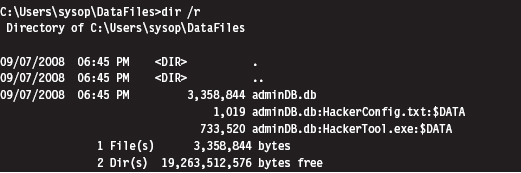
As you can see, the admin.db file has two additional data streams associated with it (neither of which affects the directory’s total file size of 3,358,844 bytes). One is a configuration file and the other is a tool of some sort. As you can see, the name of an ADS file obeys the following convention:

FileName:StreamName:$StreamType

The file name, its ADS, and the ADS type are delimited by colons. The stream type is prefixed by a dollar sign (i.e., $DATA). Another thing to keep in mind is that there are no time stamps associated with a stream. The file times associated with a file are updated when any stream in a file is updated.

The problem with using the dir command to enumerate ADSs is that the output format is difficult to work with. The ADS files are mixed in with all of the other files, and there’s a bunch of superfluous information. Thankfully there are tools like Lads.exe that format their output in a manner that’s more concise.²⁰ For example, we could use lads.exe to summarize the same exact information as the previous dir command.

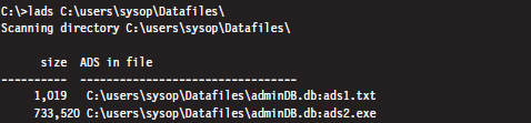
As you can see, this gives us exactly the information we seek without all of the extra fluff. We could take this a step further using the /s switch (which enables recursive queries into all subdirectories) to enumerate all of the ADS files in a given file system.

Enumerating ADSs: Countermeasures

To foil ADS enumeration, you’d be well advised to eschew ADS storage to begin with. The basic problem is that ADSs are intrinsically suspicious and will immediately arouse mistrust even if they’re completely harmless. Remember, our goal is to remain low and slow.

Recovering File System Objects

The bulk of an investigator’s data set will be derived from existing files that reside in a file system. Nothing special, really, just tens of thousands of mundane file system objects. Given the sheer number of artifacts, the investigator will need to rely on automation to speed things up.

Recovering File System Objects: Countermeasures

There are a couple of tactics that can be used to make it difficult for an investigator to access a file system’s objects. This includes:

  File system attacks.

  Encrypted volumes.

  Concealment.

File system attacks belong to the scorched earth school of AF. The basic idea is to implement wholesale destructive modification of the file system in order to prevent forensic tools from identifying files properly. As you might expect, by maiming the file system, you’re inviting the sort of instability and eye-catching behavior that rootkits are supposed to avoid to begin with, not to mention that contemporary file-carving tools don’t necessarily need the file system anyway.

Encrypted volumes present the investigator with a file system that’s not so easily carved. If a drive or logical volume has been encrypted, extracting files will be an exercise in futility (particularly if the decryption key can’t be recovered). As with file system attacks, I dislike this technique because it’s too conspicuous.

Concealment, if it’s used judiciously, can be an effective short-term strategy. The last part of the previous sentence should be emphasized. The trick to staying below the radar is to combine this tactic with some form of data transformation so that your file looks like random noise. Otherwise, the data that you’ve hidden will stand out by virtue of the fact that it showed up in a location where it shouldn’t be. Imagine finding a raw FAT file system nestled in a disk’s slack space …

In a Black Hat DC 2006 presentation,²¹ Irby Thompson and Mathew Monroe described a framework for concealing data that’s based on three different concealment strategies:

  Out-of-band concealment.

  In-band concealment.

  Application layer concealment.

These strategies are rich enough that they all deserve in-depth examination.

Out-of-Band Concealment

Out-of-band concealment places data in disk regions that are not described by the file system specification, such that the file system routines don’t normally access them. We’ve already seen examples of this with HPAs and DCOs.

Slack space is yet another well-known example. Slack space exists because the operating system allocates space for files in terms of clusters (also known as allocation units), where a cluster is a contiguous series of one or more sectors of disk space. The number of sectors per cluster and the number of bytes per sector can vary from one installation to the next. Table 7.1 specifies the default cluster sizes on an NTFS volume.

Table 7.1 Default NTFS Cluster Sizes

Volume Size	Cluster Size
Less than 512 MB	512 bytes (1 sector)
513 MB to 1 GB	1 KB
1 GB to 2 GB	2 KB
2 GB to 2 TB	4 KB

You can determine these parameters at runtime using the following code:

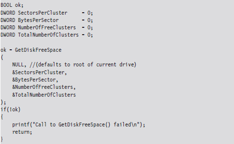
Given that the cluster is the smallest unit of storage for a file and that the data stored by the file might not always add up to an exact number of clusters, there’s bound to be a bit of internal fragmentation that results. Put another way, the logical end of the file will often not be equal to the physical end of the file, and this leads to some empty real estate on disk.

Let’s look at an example to clarify this. Assuming we’re on a system where a cluster consists of eight sectors, where each sector is 512 bytes, a text file consisting of 2,000 bytes will use less than half of its cluster. This extra space can be used to hide data (see Figure 7.9). This slack space can add up quickly, offering plenty of space for us to stow our sensitive data.

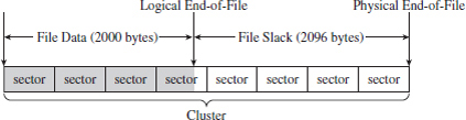
Figure 7.9

The distinction is sometimes made between RAM slack and drive slack (see Figure 7.10). RAM slack is the region that extends from the logical end of the file to the end of the last partially used sector. Drive slack is the region that extends from the start of the following sector to the physical end of the file. During file write operations, the operating system zeroes out the RAM slack, leaving only the drive slack as a valid storage space for sensitive data that we want to hide.

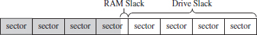
Figure 7.10

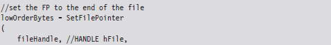
Although you may suspect that writing to slack space might require some fancy low-level acrobatics, it’s actually much easier than you think. The process for storing data in slack space uses the following recipe:

  Open the file and position the current file pointer at the logical EOF.

  Write data to the slack space (keep in mind RAM slack).

  Truncate the file, nondestructively, so that slack data is beyond the logical end of file (EOF).

This procedure relies heavily on the SetEndOfFile() routine to truncate the file nondestructively back to its original size (i.e., the file’s final logical end-of-file is the same as its original). Implemented in code, this looks something like:

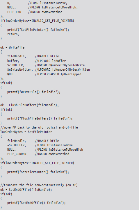
Visually, these series of steps look something like what’s depicted in Figure 7.11.

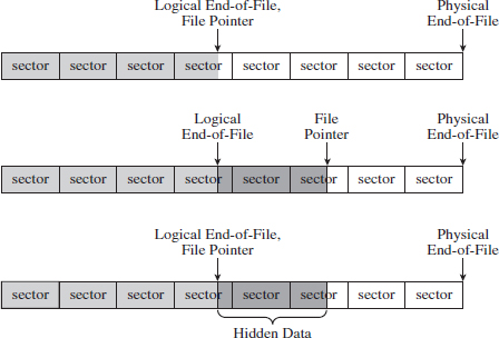
Figure 7.11

Recall that I mentioned that the OS zeroes out RAM slack during write operations. This is how things work on Windows XP and Windows Server 2003. However, on more contemporary systems, like Windows Vista, it appears that the folks in Redmond (being haunted by the likes of Vinnie Liu) wised up and have altered the OS so that it zeroes out slack space in its entirety during the call to SetEndOfFile().

This doesn’t mean that slack space can’t be used anymore. Heck, it’s still there, it’s just that we’ll have to adopt more of a low-level approach (i.e., raw disk I/O) that isn’t afforded to us in user mode. Suffice it to say that this would force us down into kernel mode (see Figure 7.12). Anyone intent on utilizing slack space using a KMD would be advised to rely on static files that aren’t subjected to frequent I/O requests, as files that grow can overwrite slack space. Given this fact, the salient issue then becomes identifying such files (hint: built-in system executables are a good place to start).

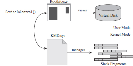
Figure 7.12

Reading slack space and wiping slack space use a process that’s actually a bit simpler than writing to slack space:

  Open the file and position the current file pointer at the logical EOF.

  Extend the logical EOF to the physical EOF.

  Read/overwrite the data between the old logical EOF and the physical EOF.

  Truncate the file back to its original size by restoring the old logical EOF.

Reading (or wiping, as the case may be) depends heavily on the SetFileValidData() routine to nondestructively expand out a file’s logical terminus (see Figure 7.13). Normally, this function is used to create large files quickly.

As mentioned earlier, the hardest part about out-of-band hiding is that it requires special tools. Utilizing slack space is no exception. In particular, a tool that stores data in slack space must keep track of which files get used and how much slack space each one provides. This slack space metadata will need to be archived in an index file of some sort. This metadata file is the Achilles’ heel of the tactic. If you lose the index file, you lose the slack data.

Although slack space is definitely a clever idea, most of the standard forensic tools can dump it and analyze it. Once more, system administrators can take proactive measures by periodically wiping the slack space on their drives.

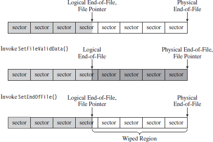
Figure 7.13

If you’re up against average Joe system administrator, using slack space can still be pulled off. However, if you’re up against the alpha geek forensic investigator whom I described at the beginning of the chapter, you’ll have to augment this tactic with some sort of data transformation and find some way to camouflage the slack space index file.

True to form, the first publicly available tool for storing data in slack space was released by the Metasploit project as a part of their Metasploit Anti-Forensic Project.²² The tool in question is called Slacker.exe, and it works like a charm on XP and Windows Server 2003, but on later versions of Windows it does not.

In-Band Concealment

In-band concealment stores data in regions that are described by the file system specification. A contemporary file system like NTFS is a veritable metropolis of data structures. Like any urban jungle, it has its share of back alleys and abandoned buildings. Over the past few years, there’ve been fairly sophisticated methods developed to hide data within different file systems. For example, the researcher known as The Grugq came up with an approach called the file insertion and subversion technique (FIST).

The basic idea behind FIST is that you find an obscure storage spot in the file system infrastructure and then find some way to use it to hide data (e.g., as The Grugq observes, the developer should “find a hole and then FIST it”). Someone obviously has a sense of humor.

Data hidden in this manner should be stable, which is to say that it should be stored such that:

  The probability of the data being overwritten is low.

  It can survive processing by a file system integrity checker.

  A nontrivial amount of data can be stored.

The Grugq went on to unleash several UNIX-based tools that implemented this idea for systems that use the Ext2 and Ext3 file system. This includes software like Runefs, KY FS, and Data Mule FS (again with the humor). Runefs hides data by storing it in the system’s “bad blocks” file. KY FS (as in, kill your file system or maybe KY Jelly) conceals data by placing it in directory files. Data Mule FS hides data by burying it in inode reserved space.²³

It’s possible to extend the tactic of FISTing to the Windows platform. The NTFS master file table (MFT) is a particularly attractive target. The MFT is the central repository for file system metadata. It’s essentially a database that contains one or more records for each file on an NTFS file system.

The location of the MFT can be determined by parsing the boot record of an NTFS volume, which I’ve previously referred to as the Windows volume boot record (VBR). According to the NTFS technical reference, the first 16 sectors of an NTFS volume (i.e., logical sectors 0 through 15) are reserved for the boot sector and boot code. If you view these sectors with a disk editor, like HxD, you’ll see that almost half of these sectors are empty (i.e., zeroed out). The layout of the first sector, the NTFS boot sector, is displayed in Figure 7.14.

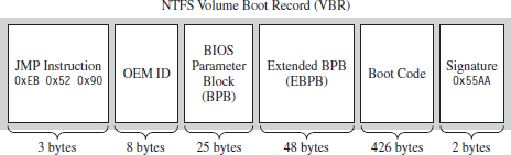
Figure 7.14

The graphical representation in Figure 7.14 can be broken down even further using the following C structure:

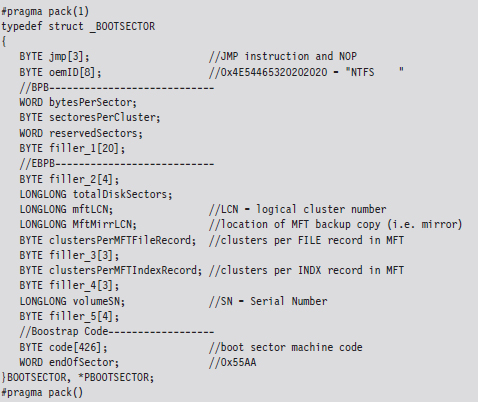
The first three bytes of the boot sector comprise two assembly code instructions: a relative JMP and a NOP instruction. At runtime, this forces the processor to jump forward 82 bytes, over the next three sections of the boot sector, and proceed straight to the boot code. The OEM ID is just an 8-character string that indicates the name and version of the OS that formatted the volume. This is usually set to “NTFS” suffixed by four space characters (e.g., 0×20).

The next two sections, the BIOS parameter block (BPB) and the extended BIOS parameter block (EBPB), store metadata about the NTFS volume. For example, the BPB specifies the volume’s sector and cluster size use. The EBPB, among other things, contains a field that stores the logical cluster number (LCN) of the MFT. This is the piece of information that we’re interested in.

Once we’ve found the MFT, we can parse through its contents and look for holes where we can stash our data. The MFT, like any other database table, is just a series of variable-length records. These records are usually contiguous (although, on a busy file system, this might not always be the case). Each record begins with a 48-byte header (see Figure 7.15) that describes the record, including the number of bytes allocated for the record and the number of those bytes that the record actually uses. Not only will this information allow us to locate the position of the next record, but it will also indicate how much slack space there is.

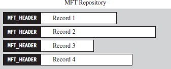
Figure 7.15

From the standpoint of a developer, the MFT record header looks like:

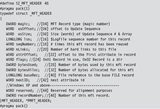
The information that follows the header, and how it’s organized, will depend upon the type of MFT record you’re dealing with. You can discover what sort of record you’re dealing with by checking the 32-bit value stored in the magic field of the MFT_HEADER structure. The following macros define nine different types of MFT records.

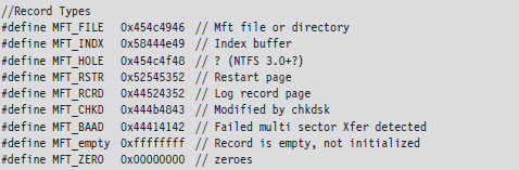
Records of type MFT_FILE consist of a header, followed by one or more variable-length attributes, and then terminated by an end marker (i.e., O×FFFFFFFF). See Figure 7.16 for an abstract depiction of this sort of record.

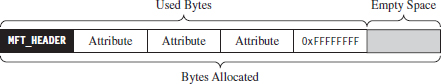
Figure 7.16

MFT_FILE records represent a file or a directory. Thus, from the vantage point of the NTFS file system, a file is seen as a collection of file attributes. Even the bytes that physically make up a file on disk (e.g., the ASCII text that appears in a configuration file or the binary machine instructions that constitute an executable) are seen as a sort of attribute that NTFS associates with the file. Because MFT records are allocated in terms of multiples of disk sectors, where each sector is usually 512 bytes in size, there may be scenarios where the number of bytes consumed by the file record (e.g., the MFT record header, the attributes, and the end marker) is less than the number of bytes initially allocated. This slack space can be used as a storage area to hide data.

Each attribute begins with a 24-byte header that describes general characteristics that are common to all attributes (this 24-byte blob is then followed by any number of metadata fields that are specific to the particular attribute). The attribute header can be instantiated using the following structure definition:

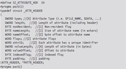
The first field specifies the type of the attribute. The following set of macros provides a sample list of different types of attributes:

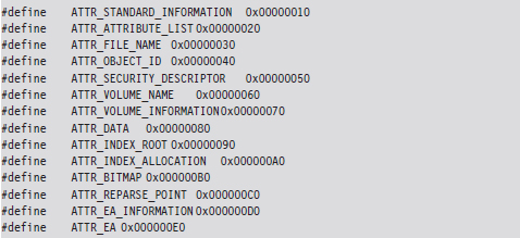
The prototypical file on an NTFS volume will include the following four attributes in the specified order (see Figure 7.17):

  The $STANDARD_INFORMATION attribute.

  The $FILE_NAME attribute.

  The $SECURITY_DESCRIPTOR attribute.

  The $DATA attribute.

Figure 7.17

The $STANDARD_INFORMATION attribute is used to store time stamps and old DOS-style file permissions. The $FILE_NAME attribute is used to store the file’s name, which can be up to 255 Unicode characters in length. The $SECURITY_ DESCRIPTOR attribute specifies the access control lists (ACLs) associated with the file and ownership information. The $DATA attribute describes the physical bytes that make up the file. Small files will sometimes be “resident,” such that they’re stored entirely in the $DATA section of the MFT record rather than being stored in external clusters outside of the MFT.

Of these four attributes, we’ll limit ourselves to digging into the $FILE_NAME attribute. This attribute is always resident, residing entirely within the confines of the MFT record. The body of the attribute, which follows the attribute header on disk, can be specified using the following structure:

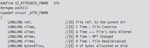
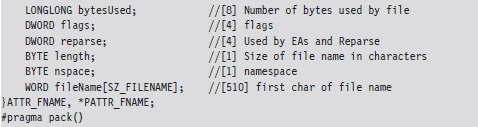
The file name will not always require all 255 Unicode characters, and so the storage space consumed by the fileName field may spill over into the following attribute. However, this isn’t a major problem because the length field will prevent us from accessing things that we shouldn’t.

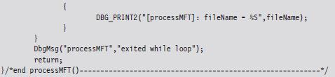
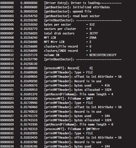
As a learning tool, I cobbled together a rather primitive KMD that walks through the MFT. It examines each MFT record and prints out the bytes used by the record and the bytes allocated by the record. In the event that the MFT record being examined corresponds to a file or directory, the driver drills down into the record’s $FILE_NAME attribute. This code makes several assumptions. For example, it assumes that MFT records are contiguous on disk, and it stops the minute it encounters a record type it doesn’t recognize. Furthermore, it only drills down into file records that obey the standard format described earlier.

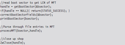
This code begins by reading the boot sector to determine the LCN of the MFT. In doing so, there is a slight adjustment that needs to be made to the boot sector’s clustersPerMFTFileRecord and clustersPerMFTIndexRecord fields. These 16-bit values represent signed words. If they’re negative, then the number of clusters allocated for each field is 2 raised to the absolute value of these numbers.

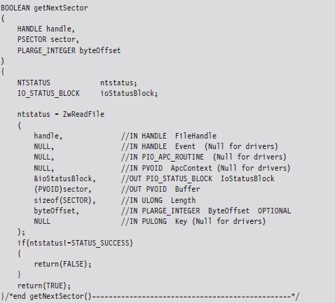
Once we know the LCN of the MFT, we can use the other parameters derived from the boot sector (e.g., the number of sectors per cluster and the number of bytes per sector) to determine the logical byte offset of the MFT. Ultimately, we can feed this offset to the ZwReadFile() system call to implement seek-and-read functionality, otherwise we’d have to make repeated calls to ZwReadFile() to get to the MFT, and this could be prohibitively expensive. Hence, the following routine doesn’t necessarily get the “next” sector, but rather it retrieves a sector’s worth of data starting at the byteOffset indicated.

After extracting the first record header from the MFT, we use the bytesAlloc field in the header to calculate the offset of the next record header. In this manner, we jump from one MFT record header to the next, printing out the content of the headers as we go. Each time we encounter a record, we check to see if the record represents an instance of a MFT_FILE. If so, we drill down into its $FILE_NAME attribute and print out its name.

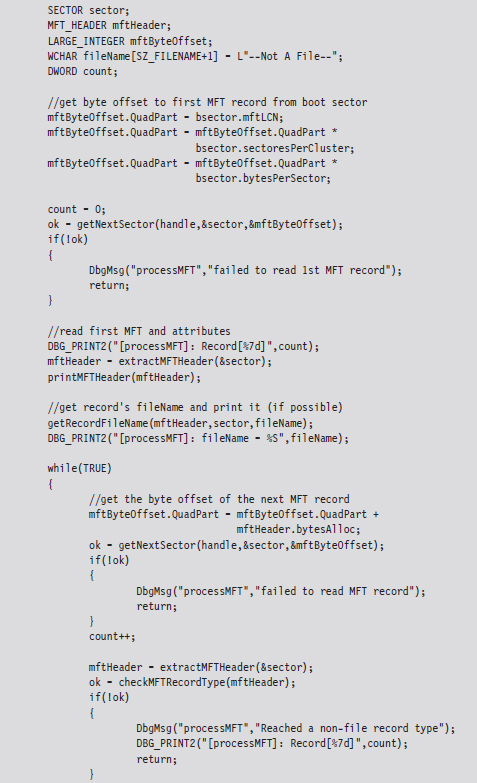
If you glance over the output generated by this code, you’ll see that there is plenty of unused space in the MFT. In fact, for many records less than half of the allocated space is used.

Despite the fact that all of these hiding spots exist, there are issues that make this approach problematic. For instance, over time a file may acquire additional ACLs, have its name changed, or grow in size. This can cause the amount of unused space in an MFT record to decrease, potentially overwriting data that we have hidden there. Or, even worse, an MFT record may be deleted and then zeroed out when it’s re-allocated.

Then there’s also the issue of taking the data from its various hiding spots in the MFT and merging it back into usable files. What’s the best way to do this? Should we use an index file like the slacker.exe tool? We’ll need to have some form of bookkeeping structure so that we know what we hid and where we hid it.

Enter: FragFS

These issues have been addressed in an impressive anti-forensics package called FragFS, which expands upon the ideas that I just presented and takes them to the next level. FragFS was presented by Irby Thompson and Mathew Monroe at the Black Hat DC conference in 2006. The tool locates space in the MFT by identifying entries that aren’t likely to change (i.e., nonresident files that haven’t been altered for at least a year). The corresponding free space is used to create a pool that’s logically formatted into 16-byte storage units. Unlike slacker.exe, which archives storage-related metadata in an external file, the FragFS tool places bookkeeping information in the last 8 bytes of each MFT record.

The storage units established by FragFS are managed by a KMD that merges them into a virtual disk that supports its own file system. In other words, the KMD creates a file system within the MFT. To quote Special Agent Fox Mulder, it’s a shadow government within the government. You treat this drive as you would any other block-based storage device. You can create directory hierarchies, copy files, and even execute applications that are stored there.

Unfortunately, like many of the tools that get demonstrated at conferences like BlackHat, the source code to the FragFS KMD will remain out of the public domain. Nevertheless, it highlights what can happen with proprietary file systems: The Black Hats uncover a loophole that the White Hats don’t know about and evade capture because the White Hats can’t get the information they need to build more effective forensic tools.

Application-Level Concealment

Application layer hiding conceals data by leveraging file-level format specifications. In other words, rather than hide data in the nooks and crannies of a file system, you identify locations inside of the files within a given file system. There are ways to subvert executable files and other binary formats so that we can store data in them without violating their operational integrity.

Although hiding data within the structural alcoves of an executable file has its appeal, the primary obstacle that stands in the way is the fact that doing so will alter the file’s checksum signature (thus alerting the forensic investigator that something is amiss). A far more attractive option would be to find a binary file that changes, frequently, over the course of the system’s normal day-to-day operation and hide our data there. To this end, databases are an enticing target. Databases that are used by the operating system are even more attractive because we know that they’ll always be available.

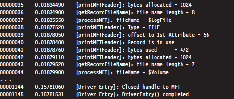
For example, the Windows Registry is the Grand Central Station of the operating system. Sooner or later, everyone passes through there. It’s noisy, it’s busy, and if you want to hide there’s even a clandestine sub-basement known as M42. There’s really no way to successfully checksum the hive files that make up the registry. They’re modified several times a second. Hence, one way to conceal a file would be to encrypt it, and then split it up into several chunks, which are stored as REG_BINARY values in the registry. At runtime these values could be re-assembled to generate the target.

You might also want to be a little more subtle with the value names that you use and then sprinkle them around in various keys so they aren’t clumped together in a single spot.

Acquiring Metadata

Having amassed as many files as possible, the forensic investigator can now collect metadata on each of the files. This includes pieces of information like:

  The file’s name.

  The full path to the file.

  The file’s size (in bytes).

  MAC times.

  A cryptographic checksum of the file.

The acronym MAC stands for modified, accessed, and created. Thus, MAC time stamps indicate when a file was last modified, last accessed, or when it was created. Note that a file can be accessed (i.e., opened for reading) without being modified (i.e., altered in some way) such that these three values can all be distinct.

If you wade into the depths of the WDK documentation, you’ll see that Windows actually associates four different time-related values with a file. The values are represented as 64-bit integer data types in the FILE_BASIC_INFORMATION structure defined in Wdm.h.

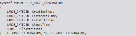
These time values are measured in terms of 100-nanosecond intervals from the start of 1601, which explains why they have to be 64 bits in size.

CreationTime	When the file was created.
LastAccessTime	When the file was last accessed (i.e., opened).
LastWriteTime	When the file’s content was last altered.
ChangeTime	When the file’s metadata was last modified.

These fields imply that a file can be changed without being written to, which might seem counterintuitive at first glance. This makes more sense when you take the metadata of the file stored in the MFT into account.

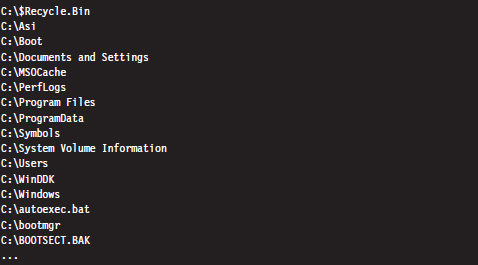
We can collect file name, path, size, and time-stamp information using the following batch file:

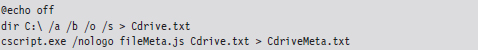
The first command recursively traverses all of the subdirectories of the C: drive. For each directory, it displays all of the subdirectories and then all of the files in bare format (including hidden files and system files).

The second command takes every file in the list created by the first command and, using Jscript as a scripting tool, prints out the name, size, and MAC times of each file. Note that this script ignores directories.

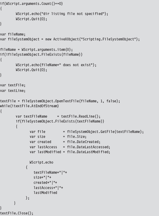
The output of this script has been delimited by vertical bars (i.e., “|”) so that it would be easier to import to Excel or some other spreadsheet application.

A cryptographic hash function is a mathematical operation that takes an arbitrary stream of bytes (often referred to as the message) and transforms it into a fixed-size integer value that we’ll refer to as the checksum (or message digest):

hash(message) → checksum.

In the best case, a hash function is a one-way mapping such that it’s extremely difficult to determine the message from the checksum. In addition, a well-designed hash function should be collision resistant. This means that it should be hard to find two messages that resolve to the same checksum.

These properties make hash functions useful with regard to verifying the integrity of a file system. Specifically, if a file is changed during some window of time, the file’s corresponding checksum should also change to reflect this modification. Using a hash function to detect changes to a file is also attractive because computing a checksum is usually cheaper than performing a byte-by-byte comparison.

For many years, the de facto hash function algorithm for verifying file integrity was MD5. This algorithm was shown to be insecure,²⁵ which is to say that researchers found a way to create two files that collided, yielding the same MD5 checksum. The same holds for SHA-1, another well-known hash algorithm.²⁶ Using an insecure hashing algorithm has the potential to make a system vulnerable to intruders who would patch system binaries (to introduce Trojan programs or back doors) or hide data in existing files using steganography.

In 2004, the International Organization for Standardization (ISO) adopted the Whirlpool hash algorithm in the ISO/IEC 10118-3:2004 standard. There are no known security weaknesses in the current version. Whirlpool was created by Vincent Rijmen and Paulo Barreto. It works on messages less than 2,256 bits in length and generates a checksum that’s 64 bytes in size.

Jesse Kornblum maintains a package called whirlpooldeep that can be used to compute the Whirlpool checksums of every file in a file system.²⁷ Although there are several, “value-added” feature-heavy, commercial packages that will do this sort of thing, Kornblum’s implementation is remarkably simple and easy to use.

For example, the following command can be used to obtain a hash signature for every file on a machine’s C: drive:

The -s switch enables silent mode, such that all error messages are suppressed. The -r switch enables recursive mode, so that all of the subdirectories under the C: drive’s root directory are processed. The results are redirected to the OldHash.txt file for archival.

To display the files on the drive that don’t match the list of known hashes at some later time, the following command can be issued:

This command uses the file checksums in OldHash.txt as a frame of reference against which to compare the current file checksum values. Files that have been modified will have their checksum and full path recorded in DoNotMatch.txt.

Acquiring Metadata: Countermeasures

One way to subvert metadata collection is by undermining the investigator’s trust in his data. Specifically, it’s possible to alter a file’s time stamp or checksum. The idea is to fake out whatever automated forensic tools the investigator is using and barrage the tools with so much contradictory data that the analyst is more inclined throw up his arms. You want to prevent the analyst from creating a timeline of events, and you also want to stymie his efforts to determine which files were actually altered to facilitate the attack. The best place to hide is in a crowd, and in this instance you basically create your own crowd.

The downside of this stratagem is that it belongs to the scorched earth school of thought. You’re creating an avalanche of false positives, and this will look flagrantly suspicious to the trained eye. Remember, our goal is to remain low and slow.

Altering Time Stamps

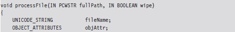
Time-stamp manipulation can be performed using publicly documented information in the WDK. Specifically, it relies upon the proper use of the ZwOpenFile() and ZwSetInformationFile() routines, which can only be invoked at an IRQL equal to PASSIVE_LEVEL.

The following sample code accepts the full path of a file and a Boolean flag. If the Boolean flag is set, the routine will set the file’s time stamps to extremely low values. When this happens, tools like the Windows Explorer will fail to display the file’s time stamps at all, showing blank fields instead.

If the Boolean flag is cleared, the time stamps of the file will be set to those of a standard system file, so that the file appears as though it has existed since the operating system was installed. The following code could be expanded upon to assign an arbitrary time stamp.

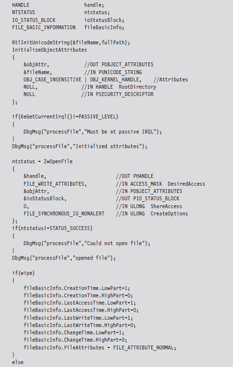
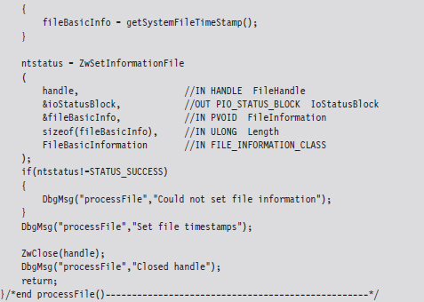
When the FILE_INFORMATION_CLASS argument to ZwSetInformationFile() is set to FileBasicInformation, the routine’s FileInformation void pointer expects the address of a FILE_BASIC_INFORMATION structure, which we met in the past chapter. This structure stores four different 64-bit LARGE_INTEGER values that represent the number of 100-nanosecond intervals since the start of 1601. When these values are small, the Windows API doesn’t translate them correctly and displays nothing instead. This behavior was publicly reported by Vinnie Liu of the Metasploit project.

Altering Checksums

The strength of the checksum is also its weakness: one little change to a file and its checksum changes. This means that we can take a normally innocuous executable and make it look suspicious by twiddling a few bytes. Despite the fact that patching an executable can be risky, most of them contain embedded character strings that can be manipulated without altering program functionality. For example, the following hex dump represents the first few bytes of a Windows application.

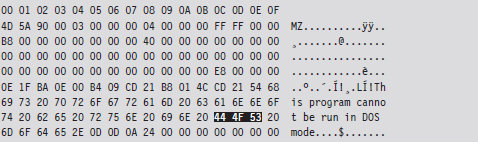
We can alter this program’s checksum by changing the word “DOS” to “dos.”

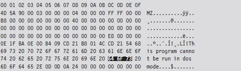
Institute this sort of mod in enough places, to enough files, and the end result is a deluge of false positives: files that, at first glance, look like they may have been maliciously altered when they actually are still relatively safe.

Identifying Known Files

By now the forensic analyst will have two snapshots of the file system. One snapshot will contain the name, full path, size, and MAC times of each file in the file system. The other snapshot will store the checksum for each file in the file system. These two snapshots, which are instantiated as ASCII text files, do an acceptable job of representing the current state of the file system.

In the best-case scenario, the forensic investigator will have access to an initial pair of snapshots, which can provide a baseline against which to compare the current snapshots. If this is the case, he’ll take the current set of files that he’s collected and begin to prune away at it by putting the corresponding metadata side by side with the original metadata. Given that the average file system can easily store 100,000 files, doing so is a matter of necessity more than anything else. The forensic analyst doesn’t want to waste time examining files that don’t contribute to the outcome of the investigation. He wants to isolate and focus on the anomalies.

One way to diminish the size of the forensic file set is to remove the elements that are known to be legitimate (i.e., known good files). This would include all of the files whose checksums and other metadata haven’t changed since the original snapshots were taken. This will usually eliminate the bulk of the candidates. Given that the file metadata we’re working with is ASCII text, the best way to do this is by a straight-up comparison. This can be done manually with a GUI program like WinMerge²⁸ or automatically from the console via the fc.exe command:

The /L option forces the fc.exe command to compare the files as ASCII text. The /N option causes the line numbers to be displayed. For cryptographic checksums, it’s usually easier to use whirlpooldeep.exe directly (instead of fc.exe or WinMerge) to identify files that have been modified.

A forensic investigator might then scan the remaining set of files with anti-virus software, or perhaps an anti-spyware suite, that uses signature-based analysis to identify objects that are known bad files (e.g., Trojans, back doors, viruses, downloaders, worms, etc.). These are malware binaries that are prolific enough that they’ve actually found their way into the signature databases of security products sold by the likes of McAfee and Symantec.

Once the known good files and known bad files have been trimmed away, the forensic investigator is typically left with a manageable set of potential suspects (see Figure 7.18). Noisy parts of the file system, like the temp directory and the recycle bin, tend to be repeat offenders. This is where the investigator stops viewing the file system as a whole and starts to examine individual files in more detail.

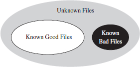
Figure 7.18

Cross-Time Versus Cross-View Diffs

The basic approach being used here is what’s known as a cross-time diff. This technique detects changes to a system’s persistent medium by comparing state snapshots from two different points in time. This is in contrast to the cross-view diff approach, where the snapshots of a system’s state are taken at the same time but from two different vantage points.

Unlike cross-view detection, the cross-time technique isn’t played out at runtime. This safeguards the forensic process against direct interference by the rootkit. The downside is that a lot can change in a file system over time, leading to a significant number of false positives. Windows is such a massive, complex OS that in just a single minute, dozens upon dozens of files can change (e.g., event logs, Prefetch files, indexing objects, registry hives, application data stores, etc.).

In the end, using metadata to weed out suspicious files is done for the sake of efficiency. Given a forensic-quality image of the original drive and enough time, an investigator could perform a raw binary comparison of the current and original file systems. This would unequivocally show which files had been modified and which files had not, even if an attacker had succeeded in patching a file and then appended the bytes necessary to cause a checksum collision. The problem with this low-tech approach is that it would be slow. In addition, checksum algorithms like Whirlpool are considered to be secure enough that collisions are not a likely threat.

Identifying Known Files: Countermeasures

There are various ways to monkey wrench this process. In particular, the attacker can:

  Move files into the known good list.

  Introduce known bad files.

  Flood the system with foreign binaries.

If the forensic investigator is using an insecure hashing algorithm (e.g., MD4, MD5) to generate file checksums, it’s possible that you could patch a preexisting file, or perhaps replace it entirely, and then modify the file until the checksum matches the original value. Formally, this is what’s known as a preimage attack. Being able to generate a hash collision opens up the door to any number of attacks (i.e., steganography, direct binary patching, Trojan programs, back doors attached via binders, etc.).

Peter Selinger, an associate professor of mathematics at Dalhousie University, has written a software tool called evilize that can be used to create MD5-colliding executables.²⁹ Marc Stevens, while completing his master’s thesis at the Eindhoven University of Technology, has also written software for generating MD5 collisions.³⁰

Another way to lead the forensic investigator away from your rootkit is to give him a more obvious target. If, during the course of his analysis, he comes across a copy of Hacker Defender or the Bobax Worm, he may prematurely conclude that he’s isolated the cause of the problem and close the case. This is akin to a pirate who buries a smaller treasure chest on top of a much larger one to fend off thieves who might go digging around for it.

The key to this defense is to keep it subtle. Make the investigator work hard enough so that when he finally digs up the malware, it seems genuine. You’ll probably need to do a bit of staging, so that the investigator can “discover” how you got on and what you did once you broke in.

Also, if you decide to deploy malware as a distraction, you can always encrypt it to keep the binaries out of reach of the local anti-virus package. Then, once you feel like your presence has been detected, you can decrypt the malware to give the investigator something to chase.

The Internet is awash with large open-source distributions, like The ACE ORB or Apache, which include literally hundreds of files. The files that these packages ship with are entirely legitimate and thus will not register as known bad files. However, because you’ve downloaded and installed them after gaining a foothold on a machine, they won’t show up as known good files, either. The end result is that the forensic investigator’s list of potentially suspicious files will balloon and consume resources during analysis, buying you valuable time.

It goes without saying that introducing known bad files on a target machine or flooding a system with known good files are both scorched earth tactics.

7.5    File Signature Analysis

---

By this stage of the game, the forensic investigator has whittled down his initial data set to a smaller collection of unknown files. His goal now will be to try and identify which of these unknown files store executable code (as opposed to a temporary data file, or the odd XML log, or a configuration file). Just because a file ends with the .txt extension doesn’t mean that it isn’t a DLL or a driver. There are tools that can be used to determine if a file is an executable despite the initial impression that it’s not. This is what file signature analysis is about.

There are commercial tools that can perform this job admirably, such as EnCase. These tools discover a file’s type using a pattern-matching approach. Specifically, they maintain a database of binary snippets that always appear in certain types of files (this database can be augmented by the user). For example, Windows applications always begin with 0x4D5A, JPEG graphics files always begin with 0×FFD8FFE0, and Adobe PDF files always begin with 0×25504446. A signature analysis tool will scan the header and the footer of a file looking for these telltale snippets at certain offsets.

On the open source side of the fence, there’s a tool written by Jesse Kornblum, aptly named Miss Identify, which will identify Win32 applications.³¹ For example, the following command uses Miss Identify to search the C: drive for executables that have been mislabeled:

Finally, there are also compiled lists of file signatures available on the Internet.³² Given the simplicity of the pattern-matching approach, some forensic investigators have been known to roll their own signature analysis tools using Perl or some other field-expedient scripting language. These tools can be just as effective as the commercial variants.

File Signature Analysis: Countermeasures

Given the emphasis placed on identifying a known pattern, you can defend against signature analysis by modifying files so that they fail to yield a match. For example, if a given forensic tool detects PE executables by looking for the “MZ” magic number at the beginning of a file, you could hoodwink the forensic tool by changing a text file’s extension to “EXE” and inserting the letters M and Z right at the start.

This sort of cheap trick can usually be exposed simply by opening a file and looking at it (or perhaps by increasing the size of the signature).

The ultimate implementation of a signature analysis countermeasure would be to make text look like an executable by literally embedding the text inside of a legitimate, working executable (or some other binary format). This would be another example of application layer hiding, and it will pass all forms of signature analysis with flying colors.

Notice how I’ve enclosed the encoded text inside of XML tags so that the information is easier to pick out of the compiled binary.

The inverse operation is just as plausible. You can take an executable and make it look like a text file by using something as simple as the Multipurpose Internet Mail Extensions (MIME) base64 encoding scheme. If you want to augment the security of this technique, you could always encrypt the executable before base64 encoding it.

Taking this approach to the next level of sophistication, there has actually been work done to express raw machine instructions so that they resemble written English.³³

7.6    Conclusions

---

This ends the first major leg of the investigation. What we’ve seen resembles a gradual process of purification. We start with a large, uncooked pile of data that we send through a series of filters. At each stage we refine the data, breaking it up into smaller pieces and winnowing out stuff that we don’t need. What we’re left with in the end is a relatively small handful of forensic pay dirt.

The investigator started with one or more hard drives, which he duplicated. Then he used his tools to decompose the forensic duplicates into a series of volumes that host individual file systems. These file systems are like sponges, and the investigator wrings them out as best he can to yield the largest possible collection of files (and maybe even fragments of files).

Given the resulting mountain of files, the investigator seeks to focus on anomalies. To this end, he acquires the metadata associated with each file and compares it against an initial system snapshot (which he’ll have if he’s lucky). This will allow him to identify and discard known files from his list of potential suspects by comparing the current metadata snapshot against the original.

At this point, the investigator will have a much smaller set of unknown files. He’ll use signature analysis to figure out which of these anomalous files is an executable. Having completed file signature analysis, the investigator will take the final subset of executables and dissect them using the methodology of the next chapter.

 

---

  1. http://www.guidancesoftware.com/computer-forensics-ediscovery-software-digital-evidence.htm.

  2. http://www.accessdata.com/forensictoolkit.html.

  3. http://dcfldd.sourceforge.net/.

  4. http://www.accessdata.com/downloads/.

  5. http://www.sleuthkit.org/.

  6. ftp://ftp.symantec.com/public/english_us_canada/tools/pq/utilities/PTEDIT32.zip.

  7. http://packages.debian.org/sid/gpart.

  8. http://www.cgsecurity.org/wiki/TestDisk.

  9. http://theinvisiblethings.blogspot.com/2006/10/vista-rc2-vs-pagefile-attack-and-some.html.

10. http://support.microsoft.com/kb/942448.

11. http://support.microsoft.com/kb/100027.

12. http://www.quetek.com.

13. http://www.sleuthkit.org/sleuthkit/.

14. http://foremost.sourceforge.net/.

15. Richard Kissel, Matthew Scholl, Steven Skolochenko, and Xing Li, Special Publication 800-88: Guidelines for Media Sanitization, National Institute of Standards and Technology, September 2006.

16. R. Sekar and A.K. Pujari (eds.): 4th International Conference on Information Systems Securing Lecture Notes in Computer Science, Vol. 5352, Springer-Verlag, Berlin, Heidelberg, 2008, pp. 243–257.

17. http://cmrr.ucsd.edu/people/Hughes/SecureErase.shtml.

18. http://gnuwin32.sourceforge.net/packages/coreutils.htm.

19. Grugq, “Defeating Forensic Analysis on Unix,” Phrack, Volume 11, Issue 59.

20. http://www.heysoft.de/en/software.php.

21. http://www.blackhat.com/presentations/bh-federal-06/BH-Fed-06-Thompson/BH-Fed-06-Thompson-up.pdf.

22. http://www.metasploit.com/research/projects/antiforensics/.

23. The Grugq, The Art of Defiling: Defeating Forensic Analysis, Black Hat 2005, United States.

24. http://www.linux-ntfs.org/doku.php.

25. Xiaoyun Wang and Hongbo Yu, “How to Break MD5 and Other Hash Functions.” In EUROCRYPT 2005, LNCS 3494, pp. 19–35, Springer-Verlag, 2005.

26. Xiaoyun Wang, Yiqun Lisa Yin, and Hongbo Yu, “Finding Collisions in the Full SHA-1.” In Advances in Cryptology - CRYPTO 2005: 25th Annual International Cryptology Conference, Springer, 2005, ISBN 3-540-28114-2.

27. http://md5deep.sourceforge.net/.

28. http://winmerge.org/.

29. http://www.mscs.dal.ca/~selinger/md5collision/.

30. http://code.google.com/p/hashclash/.

31. http://missidentify.sourceforge.net/.

32. http://www.garykessler.net/library/file_sigs.html.

33. http://www.cs.jhu.edu/~sam/ccs243-mason.pdf.