Table of Contents for
Data Analysis with Open Source Tools
 Data Analysis with Open Source Tools
Published by
O'Reilly Media, Inc., 2010
Data Analysis with Open Source Tools
Published by
O'Reilly Media, Inc., 2010
- Cover
- Data Analysis with Open Source Tools
- O'Reilly Strata Conference
- Data Analysis with Open Source Tools
- Dedication
- A Note Regarding Supplemental Files
- Preface
- 1. Introduction
- I. Graphics: Looking at Data
- 2. A Single Variable: Shape and Distribution
- 3. Two Variables: Establishing Relationships
- 4. Time As a Variable: Time-Series Analysis
- 5. More Than Two Variables: Graphical Multivariate Analysis
- 6. Intermezzo: A Data Analysis Session
- II. Analytics: Modeling Data
- 7. Guesstimation and the Back of the Envelope
- 8. Models from Scaling Arguments
- 9. Arguments from Probability Models
- 10. What You Really Need to Know About Classical Statistics
- 11. Intermezzo: Mythbusting—Bigfoot, Least Squares, and All That
- III. Computation: Mining Data
- 12. Simulations
- 13. Finding Clusters
- 14. Seeing the Forest for the Trees: Finding Important Attributes
- 15. Intermezzo: When More Is Different
- IV. Applications: Using Data
- 16. Reporting, Business Intelligence, and Dashboards
- 17. Financial Calculations and Modeling
- 18. Predictive Analytics
- 19. Epilogue: Facts Are Not Reality
- A. Programming Environments for Scientific Computation and Data Analysis
- B. Results from Calculus
- C. Working with Data
- D. About the Author
- Index
- About the Author
- Colophon
- Copyright
Chapter 18. Predictive Analytics
DATA ANALYSIS CAN TAKE MANY DIFFERENT FORMS—NOT ONLY IN THE TECHNIQUES THAT WE APPLY BUT ALSO in the kind of results that we ultimately achieve. Looking back over the material that we have covered so far, we see that the results obtained in Part I were mostly descriptive: we tried to figure out what the data was telling us and to describe it. In contrast, the results in Part II were primarily prescriptive: data was used as a guide for building models which could then be used to infer or prescribe phenomena, including effects that had not actually been observed yet. In this form of analysis, data is not used directly; instead it is used only indirectly to guide (and verify) our intuition when building models. Additionally, as I tried to stress in those chapters, we don’t just follow data blindly, but instead we try to develop an understanding of the processes that generate the data and to capture this understanding in the models we develop. The predictive power of such models derives from this understanding we develop by studying data and the circumstances in which it is generated.[30]
In this chapter, we consider yet another way to use data—we can call it predictive, since the purpose will be to make predictions about future events. What is different is that now we try to make predictions directly from the data without necessarily forming the kind of conceptual model (and the associated deeper understanding of the problem domain) as discussed in Part II. This difference is obviously both a strength and a weakness. It’s a strength in that it enables us to deal with problems for which we have no hope of developing a conceptual model, given the complexity of the situation. It is also a weakness because we may end up with only a black-box solution and no deeper understanding.
There are technical difficulties also: this form of analysis tends to require huge data sets because we are lacking the consistency and continuity guarantees provided by a conceptual model. (We will come back to this point.)
Topics in Predictive Analytics
The phrase predictive analytics is a bit of an umbrella term (others might say: marketing term) for various tasks that share the intent of deriving predictive information directly from data. Three different specific application areas stand out:
Classification or supervised learning
Assign each record to exactly one of a set of predefined classes. For example, classify credit card transactions as “valid” or “fraudulent.” Spam filtering is another example. Classification is considered “supervised,” because the classes are known ahead of time and don’t need to be inferred from the data. Algorithms are judged on their ability to assign records to the correct class.
Clustering or unsupervised learning
Group records into clusters, where the size and shape—and often even the number—of clusters is unknown. Clustering is considered “unsupervised,” because no information about the clusters is available ahead of the clustering procedure.
Recommendation
Recommend a suitable item based on past interest or behavior. Recommendation can be seen as a form of clustering, where you start with an anchor and then try to find items that are similar or related to it.
A fourth topic that is sometimes included is time-series forecasting. However, I find that it does not share many characteristics with the other three, so I usually don’t consider it part of predictive analytics itself. (We discussed time-series analysis and forecasting in Chapter 4.)
Of the three application areas, classification is arguably the most important and the best developed; the rest of this chapter will try to give an overview over the most important classification algorithms and techniques. We discussed unsupervised learning in Chapter 13 on clustering techniques—and I’ll repeat my impression that clustering is more an exploratory than a predictive technique. Recommendations are the youngest branch of predictive analytics and quite different from the other two. (There are at least two major differences. First, on the technical side, many recommendation techniques boil down to network or graph algorithms, which have little in common with the statistical techniques used for classification and clustering. Second, recommendations tend to be explicitly about predicting human behavior; this poses additional difficulties not shared by systems that follow strictly deterministic laws.) For these reasons, I won’t have much to say about recommendation techniques here.
Let me emphasize that this chapter can serve only as an overview of classification. Entire books could (and have!) been written about it. But we can outline the problem, introduce some terminology, and give the flavor of different solution approaches.
Some Classification Terminology
We begin with a data set containing multiple elements, records, or instances. Each instance consists of several attributes or features. One of the features is special: it denotes the record’s class and is known as the class label. Each record belongs to exactly one class.
A large number of classification problems are binary, consisting only of two classes (valid or fraudulent, spam or not spam); however, multiclass scenarios do also occur. Many classification algorithms can deal only with binary problems, but this is not a real limitation because any multiclass problem can be treated as a set of binary problems (belongs to the target class or does belong to any other class).
A classifier takes a record (i.e., a set of attribute values) and produces a class label for this record. Building and using a classifier generally follows a three-step process of training, testing, and actual application.
We first split the existing data set into a training set and a test set. In the training phase, we present each record from the training set to the classification algorithm. Next we compare the class label produced by the algorithm to the true class label of the record in question; then we adjust the algorithm’s “parameters” to achieve the greatest possible accuracy or, equivalently, the lowest possible error rate. (Of course, the details of this “fitting” process vary greatly from one algorithm to the next; we will look at different ways of how this is done in the next section.)
The results can be summarized in a so-called confusion matrix whose entries are the number of records in each category. (Table 18-1 shows the layout of a generic confusion matrix.)
Unfortunately, the error rate derived from the training set (the training error) is typically way too optimistic as an indicator of the error rate the classifier would achieve on new data—that is, on data that was not used during the learning phase. This is the purpose of the test set: after we have optimized the algorithm using only the training data, we let the classifier operate on the elements of the test set to see how well it classifies them. The error rate obtained in this way is the generalization error and is a much more reliable indicator of the accuracy of the classifier.
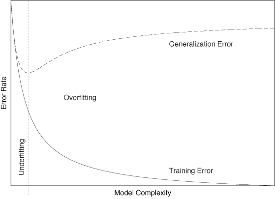
To understand the need for a separate testing phase (using a separate data set!), keep in mind that as long as we use enough parameters (i.e., making the classifier more and more complex) we can always tweak a classifier until it works very well on the training set. But in doing so, we train the classifier to memorize every aspect of the training set, including those that are atypical for the system in general. We therefore need to find the right level of complexity for the classifier. On the one hand, if it is too simple, then it cannot represent the desired behavior very well, and both its training and generalization error will be poor; this is known as underfitting. On the other hand, if we make the classifier too complex, then it will perform very well on the training set (low training error) but will not generalize well to unknown data points (high generalization error); this is known as overfitting. Figure 18-1 summarizes these concepts.
Once a classifier has been developed and tested, it can be used to classify truly new and unknown data points—that is, data points for which the correct class label is not known. (This is in contrast to the test set, where the class labels were known but not used by the classifier when making a prediction.)
Algorithms for Classification
At least half a dozen different families of classification algorithms have been developed. In this section, we briefly characterize the basic idea underlying each algorithm, emphasizing how it differs from competing methods. The first two algorithms (nearest-neighbor and Bayesian classifiers) are simpler, both technically and conceptually, than the other; I discuss them in more detail since you may want to implement them yourself. For the other algorithms, you probably want to use existing libraries instead!
Instance-Based Classifiers and Nearest-Neighbor Methods
The idea behind instance-based classifiers is dead simple: to classify an unknown instance, find an existing instance that is “most similar” to the new instance and assign the class label of the known instance to the new one!
This basic idea can be generalized in a variety of ways. First of all, the notion of “most similar” brings us back to the notion of distance and similarity measures introduced in Chapter 13; obviously we have considerable flexibility in the choice of which distance measure to use. Furthermore, we don’t have to stop at a single “most similar” existing instance. We might instead take the nearest k neighbors and use them to classify the new instance, typically by using a majority rule (i.e., we assign the new instance to the class that occurs most often among the k neighbors). We could even employ a weighted-majority rule whereby “more similar” neighbors contribute more strongly than those farther away.
Instance-based classifiers are atypical in that they don’t have a separate “training” phase; for this reason, they are also known as “lazy learners.” (The only adjustable parameter is the extent k of the neighborhood used for classification.) However, a (possibly large) set of known instances must be kept available during the final application phase. For the same reason, classification can be relatively expensive because the set of existing instances must be searched for appropriate neighbors.
Instance-based classifiers are local: they do not take the overall distribution of points into account. Additionally, they impose no particular shape or geometry on the decision boundaries that they generate. In this sense they are especially flexible. On the other hand, the are also susceptible to noise.
Finally, instance-based classifiers depend on the proper choice of distance measure, much as clustering algorithms do. We encountered this situation before, when we discussed the need for scale normalization in Chapter 13 and Chapter 14; the same considerations apply here as well.
Bayesian Classifiers
A Bayesian classifier takes a probabilistic (i.e., nondeterministic) view of classification. Given a set of attributes, it calculates the probability of the instance to belong to this or that class. An instance is then assigned the class label with the highest probability.
A Bayesian classifier calculates a conditional probability. This is the probability of the instance to belong to a specific class C, given the set of attribute values:
P(class C| {x1, x2, x3,..., xn})
Here C is the class label, and the set of attribute values is {x1, x2, x3,..., xn}. Note that we don’t yet know the value of the probability—if we did, we’d be finished.
To make progress, we invoke Bayes’ theorem (hence the name of the classifier—see also Chapter 10 for a discussion of Bayes’ theorem) to invert this probability expression as follows:
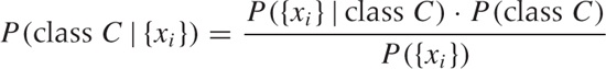
where I have collapsed the set of n features into {xi} for brevity.
The first term in the numerator (the likelihood) is the probability of observing a set of features {xi} if the instance belongs to class C (in the language of conditional probability: given the class label C). We can find an empirical value for this probability from the set of training instances: it is simply the frequency with which we observe the set of specific attribute values {xi} among instances belonging to class C. Empirically, we can approximate this distribution by a set of histograms of the {xi }, one for each class label. The second term in the numerator, P(class C), is the prior probability of any instance belonging to class C. We can estimate this probability from the fraction of instances in the training set that belong to class C. The denominator does not depend on the class label and—as usual with Bayesian computations—is ignored until the end, when the probabilities are normalized.
Through the use of Bayes’ theorem, we have been able to express the probability for an instance to belong to class C, given a set of features, entirely through expressions that can be determined from the training set.
At least in theory. In practice, it will be almost impossible to evaluate this probability directly. Look closely at the expression (now written again in its long form), P({x1, x2, x3,..., xn} | class C). For each possible combination of attribute values, we must have enough examples in our training set to be able to evaluate their frequency with some degree of reliability. This is a combinatorial nightmare! Assume that each feature is binary (i.e., it can take on one of only two values). The number of possible combinations is then 2n, so for n = 5 we already have 32 different combinations. Let’s say we need about 20 example instances for each possible combination in order to evaluate the frequency, then we’ll need a training set of at least 600 instances. In practice, the problem tends to be worse because features frequently can take more than two values, the number of features can easily be larger than five, and—most importantly—some combinations of features occur much less frequently than others. We therefore need a training set large enough to guarantee that even the least-frequent attribute combination occurs sufficiently often.
In short, the “brute force” approach of evaluating the likelihood function for all possible feature combinations is not feasible for problems of realistic size. Instead, one uses one of two simplifications.
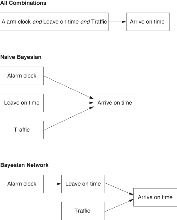
The naive Bayesian classifier assumes that all features are independent of each other, so that we can write:
P({x1, x2, x3,..., xn} |C) = P(x1|C)P(x2|C)P(x3|C) ··· P(xn|C)
This simplifies the problem greatly, because now we need only determine the frequencies for each attribute value for a single attribute at a time. In other words, each probability distribution P(xi |C) is given as the histogram of a single feature xi, separately for each class label. Despite their simplicity, naive Bayesian classifiers are often surprisingly effective. (Many spam filters work this way.)
Another idea is to use a Bayesian network. Here we prune the set of all possible feature combinations by retaining only those that have a causal relationship with each other.
Bayesian networks are best discussed through an example. Suppose we want to build a classifier that predicts whether we will be late to work in the morning, based on three binary features:
Alarm clock went off: Yes or No
Left the house on time: Yes or No
Traffic was bad: Yes or No
Although we don’t assume that all features are independent (as we did for the naive Bayesian classifier), we do observe that the traffic situation is independent of the other two features. Furthermore, whether we leave the house on time does depend on the proper working of the alarm clock. In other words, we can split the full probability:
P(Arrive on time | Alarm clock, Leave on time, Traffic)
into the following combination of events:
P(Arrive on time | Leave on time)
P(Leave on time | Alarm clock)
P(Arrive on time | Traffic)
Notice that only two of the terms give the probability for the class label (“Arrive on time”) and that one gives the probability of an intermediate event (see Figure 18-2).
For such a small example (containing only three features), the savings compared with maintaining all feature combinations are not impressive. But since the number of combinations grows exponentially with the number of features, restricting our attention to only those factors that have a causal relationship with each other can significantly reduce the number of combinations we need to retain for larger problems.
The structure (or topology) of a Bayesian network is usually not inferred from the data; instead, we use domain knowledge to determine which pathways to keep. This is exactly what we did in the example: we “knew” that traffic conditions were independent of the situation at home and used this knowledge to prune the network accordingly.
There are some practical issues that need to be addressed when building Bayesian classifiers. The description given here silently assumes that all attributes are categorical (i.e., take on only a discrete set of values). Attributes that take on continuous numerical values either need to be discretized, or we need to find the probability P({xi} | C) through a kernel density estimate (see Chapter 2) for all the points in class C in the training set. If the training set is large, the latter process may be expensive.
Another tricky detail concerns attribute values that do not occur in the training set: the corresponding probability is 0. But a naive Bayesian classifier consists of a product of probabilities and therefore becomes 0 as soon as a single term is 0! In particular with small training sets, this is a problem to watch out for. On the other hand, naive Bayesian classifiers are robust with regard to missing features: when information about an attribute value is unknown for some of the instances, the corresponding probability simply evaluates to 1 and does not affect the final result.
Regression
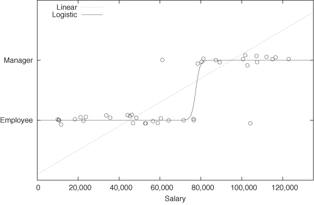
Sometimes we have reason to believe that there is a functional relationship between the class label and the set of features. For example, we might assume that there is some relationship between an employee’s salary and his status (employee or manager). See Figure 18-3.
If it is reasonable to assume a functional relationship, then we can try to build a classifier based on this relationship by “fitting” an appropriate function to the data. This turns the classification problem into a regression problem.
However, as we can see in Figure 18-3, a linear function is usually not very appropriate because it takes on all values, whereas class labels are discrete. Instead of fitting a straight line, we need something like a step function: a function that is 0 for points belonging to the one class, and 1 for points belonging to the other class. Because of its discontinuity, the step function is hard to work with; hence one typically uses the logistic function (see Appendix B) as a smooth approximation to the step function. The logistic function gives this technique its name: logistic regression. Like all regression methods, it is a global technique that tries to optimize a fit over all points and not just over a particularly relevant subset.
Logistic regression is not only important in practical applications but has deep roots in theoretical statistics as well. Until the arrival of support vector machines, it was the method of choice for many classification problems.
Support Vector Machines
Support vector machines are a relative newcomer among classification methods. The name is a bit unfortunate: there is nothing particularly “machine-y” about them. They are, in fact, based on a simple geometrical construction.
Consider training instances in a two-dimensional feature space like the one in Figure 18-4. Now we are looking for the “best” dividing line (or decision boundary) that separates instances belonging to one class from instances belonging to the other.
We need to decide what we mean by “best.” The answer given by support vector machines is that the “best” dividing line is one that has the largest margin. The margin is the space, parallel to the decision boundary, that is free of any training instances. Figure 18-4 shows two possible decision boundaries and their respective margins. Although this example is only two-dimensional, the reasoning generalizes directly to higher dimensions. In such cases, the decision boundary becomes a hyperplane, and support vector machines therefore find the maximum margin hyperplanes (a term you might find in the literature).
I will not go through the geometry and algebra required to construct a decision boundary from a data set, since you probably don’t want to implement it yourself, anyway. (The construction is not difficult, and if you have some background in analytic geometry, you will be able to do it yourself or look it up elsewhere.) The important insight is that support vector machines turn the task of finding a decision boundary first into the geometric task of constructing a line (or hyperplane) from a set of points (this is an elementary task in analytic geometry). The next step—find the decision boundary with the largest margin—is then just a multi-dimensional optimization problem, with a particularly simple and well-behaved objective function (namely, the square of the distance of each point from the decision boundary), for which good numerical algorithms exist.
One important property of support vector machines is that they perform a strict global optimization without having to rely on heuristics. Because of the nature of the objective function, the algorithm is guaranteed to find the global optimum, not merely a local one. On the other hand, the final solution does not depend on all points; instead it depends only on those closest to the decision boundary, points that lie right on the edge of the margin. (These are the support vectors, see Figure 18-4.) This means that the decision boundary depends only on instances close to it and is not influenced by system behavior far from the decision boundary. However, the global nature of the algorithm implies that, for those support vectors, the optimal hyperplane will be found!
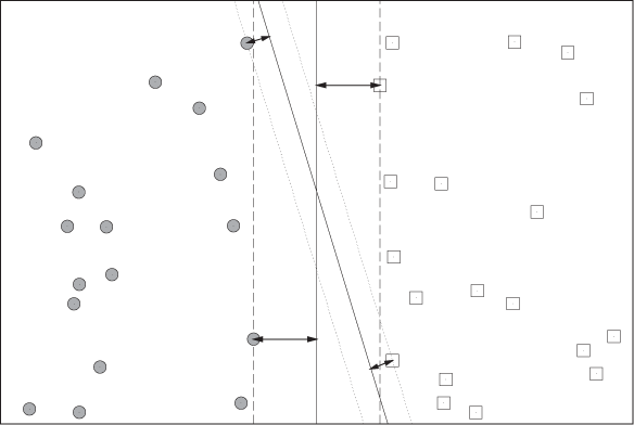
Two generalizations of this basic concept are of great practical importance. First, consider Figure 18-4 again. We were lucky that we could find a straight line (in fact, more than one) to separate the data points exactly into two classes, so that both decision boundaries shown have zero training error. In practice, it is not guaranteed that we will always find such a decision boundary, and there may be some stray instances that cannot be classified correctly by any straight-line decision boundary. More generally, it may be advantageous to have a few misclassified training instances—in return for a much wider margin—because it is reasonable to assume that a larger margin will lead to a lower generalization error later on. In other words, we want to find a balance between low training error and large margin size. This can be done by introducing slack variables. Basically, they associate a cost with each misclassified instance, and we then try to solve the extended optimization problem, in which we try to minimize the cost of misclassified instances while at the same time trying to maximize the margins.
The other important generalization allows us to use curves other than straight lines as decision boundaries. This is usually achieved through kernelization or the “kernel trick.” The basic idea is that we can replace the dot product between two vectors (which is central to the geometric construction required to find the maximum margin hyperplane) with a more general function of the two vectors. As long as this function meets certain requirements (you may find references to “Mercer’s theorem” in the literature), it can be shown that all the previous arguments continue to hold.
One disadvantage of support vector machines is that they lead to especially opaque results: they truly are black boxes. The final classifier may work well in practice, but it does not shed much light on the nature of the problem. This is in contrast to techniques such as regression or decision trees (see the next section), which often lead to results that can be interpreted in some form. (In regression problems, for instance, one can often see which attributes are the most influential ones, and which are less relevant.)
Decision Trees and Rule-Based Classifiers
Decision trees and rule-based classifiers are different from the classifiers discussed so far in that they do not require a distance measure. For this reason, they are sometimes referred to as nonmetric classifiers.
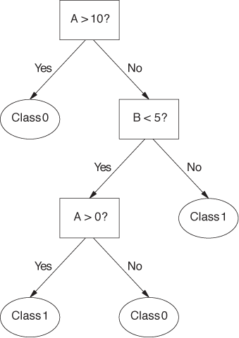
Decision trees consist of a hierarchy of decision points (the nodes of the tree). When using a decision tree to classify an unknown instance, a single feature is examined at each node of the tree. Based on the value of that feature, the next node is selected. Leaf nodes on the tree correspond to classes; once we have reached a leaf node, the instance in question is assigned the corresponding class label. Figure 18-5 shows an example of a simple decision tree.
The primary algorithm (Hunt’s algorithm) for deriving a decision tree from a training set employs a greedy approach. The algorithm is easiest to describe when all features are categorical and can take only one of two values (binary attributes). If this is the case, then the algorithm proceeds as follows:
For each instance in the training set, examine each feature in turn.
Split the training instances into two subsets based on the value of the current feature.
Select the feature that results in the “purest” subsets; the value of this attribute will be the decision condition employed by the current node.
Repeat this algorithm recursively on the two subsets until the resulting subsets are sufficiently pure.
To make this concrete, we must be able to measure the purity of a set. Let fC be the fraction of instances in the set belonging to class C. Obviously, if fC = 1 for any class label C, then the set is totally pure because all of its elements belong to the same class. We can therefore define the a purity of a set as the frequency of its most common constituent. (For example, if a set consists of 60 percent of items from class A, 30 percent from class B, and 10 percent from class C, then its purity is 60 percent.) This is not the only way to define purity. Other ways of measuring it are acceptable provided they reach a maximum when all elements of a set belong to the same class and reach a minimum when the elements of the set are distributed uniformly across classes.
Another important quantity related to decision trees is the gain ratio Δ from a parent node to its children. This quantity measures the gain in purity from parent to children, weighted by the relative size of the subsets:
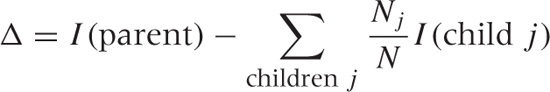
where I is the purity (or impurity) of a node, Nj is the number of elements assigned to child node j, and N is the total number of elements at the parent node. We want to find a splitting that maximizes this gain ratio.
What I have described so far is the outline of the basic algorithm. As with all greedy algorithms, there is no guarantee that it will find the optimal solution, and therefore various heuristics play a large role to ensure that the solution is as good as possible. Hence the various published (and proprietary) algorithms for decision trees (you may find references to CART, C4.5, and ID3) differ in such details such as the following:
What choice of purity/impurity measure is used?
At what level of purity does the splitting procedure stop? (Continuing to split a training set until all leaf nodes are entirely pure usually results in overfitting.)
Is the tree binary, or can a node have more than two children?
How should noncategorical attributes be treated? (For attributes that take on a continuum of values, we need to define the optimal splitting point.)
Is the tree postprocessed? (To reduce overfitting, some algorithms employ a pruning step that attempts to eliminate leaf nodes having too few elements.)
Decision trees are popular and combine several attractive features: with good algorithms, decision trees are relatively cheap to build and are always very fast to evaluate. They are also rather robust in the presence of noise. It can even be instructive to examine the decision points of a decision tree, because they frequently reveal interesting information about the distribution of class labels (such as when 80 percent of the class information is contained in the topmost node). However, algorithms for building decision trees are almost entirely black-box and do not lend themselves to ad hoc modifications or extensions.
There is an equivalence between decision trees and rule-based classifiers. The latter consist of a set of rules (i.e., logical conditions on attribute values) that, when taken in aggregate, determine the class label of a test instance. There are two ways to build a rule-based classifier. We can build a decision tree first and then transform each complete path through the decision tree into a single rule. Alternatively, we can build rule-based classifiers directly from a training set by finding a subset of instances that can be described by a simple rule. These instances are then removed from the training set, and the process is repeated. (This amounts to a bottom-up approach, whereas using a variant of Hunt’s algorithm to build a decision-tree follows a top-down approach.)
Other Classifiers
In addition to the classifiers discussed so far, you will find others mentioned in the literature. I’ll name just two—mostly because of their historical importance.
Fisher’s linear discriminant analysis (LDA) was one of the first classifiers developed. It is similar to principal component analysis (see Chapter 14). Whereas in PCA, we introduce a new coordinate system to maximize the spread along the new coordinates axes, in LDA we introduce new coordinates to maximize the separation between two classes that we try to distinguish. The position of the means, calculated separately for each class, are taken as the location of each class.
Artificial neural networks were conceived as extremely simplified models for biological brains. The idea was to have a network of nodes; each node receives input from several other nodes, forms a weighted average of its input, and then sends it out to the next layer of nodes. During the learning stage, the weights used in the weighted average are adjusted to minimize training error. Neural networks were very popular for a while but have recently fallen out of favor somewhat. One reason is that the calculations required are more complicated than for other classifiers; another is that the whole concept is very ad hoc and lacks a solid theoretical grounding.
The Process
In addition to the primary algorithms for classification, various techniques are important for dealing with practical problems. In this section, we look at some standard methods commonly used to enhance accuracy—especially for the important case when the most “interesting” type of class occurs much less frequently than the other types.
Ensemble Methods: Bagging and Boosting
The term ensemble methods refers to a set of techniques for improving accuracy by combining the results of individual or “base” classifiers. The rationale is the same as when performing some experiment or measurement multiple times and then averaging the results: as long as the experimental runs are independent, we can expect that errors will cancel and that the average will be more accurate than any individual trial. The same logic applies to classification techniques: as long as the individual base classifiers are independent, combining their results will lead to cancellation of errors and the end result will have greater accuracy than the individual contributions.
To generate a set of independent classifiers, we have to introduce some randomness into the process by which they are built. We can manipulate virtually any aspect of the overall system: we can play with the selection of training instances (as in bagging and boosting), with the selection of features (often in conjunction with random forests), or with parameters that are specific to the type of classifier used.
Bagging is an application of the bootstrap idea (see Chapter 12) to classification. We generate additional training sets by sampling with replacement from the original training set. Each of these training sets is then used to train a separate classifier instance. During production, we let each of these instances provide a separate assessment for each item we want to classify. The final class label is then assigned based on a majority vote or similar technique.
Boosting is another technique to generate additional training sets using a bootstrap approach. In contrast to bagging, boosting is an iterative process that assigns higher weights to instances misclassified in previous rounds. As the iteration progresses, higher emphasis is placed on training instances that have proven hard to classify correctly. The final result consists of the aggregate result of all base classifiers generated during the iteration. A popular variant of this technique is known as “AdaBoost.”
Random forests apply specifically to decision trees. In this technique, randomness is introduced not by sampling from the training set but by randomly choosing what features to use when building the decision tree. Instead of examining all features at every node to find the feature that gives the greatest gain ratio, only a subset of features is evaluated for each tree.
Estimating Prediction Error
Earlier, we already talked about the difference between the training and the generalization error: the training error is the final error rate that the classifier achieves on the training set. It is usually not a good measure for the accuracy of the classifier on new data (i.e., on data that was not used to train the classifier). For this reason, we hold some of the data back during training, and use it later as a test set. The error that the classifier achieves on this test set is a much better measure for the generalization error that we can expect when using the classifier on entirely new data.
If the original data set is very large, there is no problem in splitting it into a training and a test set. In reality, however, available data sets are always “too small,” so that we need to make sure we use the available data most efficiently, using a process known as cross-validation.
The basic idea is that we randomly divide the original data set into k equally sized chunks. We then perform k training and test runs. In each run, we omit one of the chunks from the training set and instead use it as the test set. Finally, we average the generalization errors from all k runs to obtain the overall expected generalization error.
A value of k = 10 is typical, but you can also use a value like k = 3. Setting k = n, where n is the number of available data points, is special: in this so-called “leave-one-out” cross-validation, we train the classifier on all data points except one and then try to predict the omitted data point—this procedure is then repeated for all data points. (This prescription is similar to the jackknife process that was mentioned briefly in Chapter 12.)
Yet another method uses the idea of random sampling with replacement, which is characteristic of bootstrap techniques (see Chapter 12). Instead of dividing the available data into k nonoverlapping chunks, we generate a bootstrap sample by drawing n data points with replacement from the original n data points. This bootstrap sample will contain some of the data points more than once, and some not at all: overall, the fraction of the unique data points included in the bootstrap sample will be about 1 – e–1 ≈ 0.632 of the available data points—for this reason, the method is often known as the 0.632 bootstrap. The bootstrap sample is used for training, and the data points not included in the bootstrap sample become the test set. This process can be repeated several times, and the results averaged as for cross-validation, to obtain the final estimate for the generalization error.
(By the way, this is basically the “unique visitor” problem
that we discussed in Chapter 9 and Chapter 12—after n days (draws)
with one random visitor each day (one data point selected per draw),
we will have seen 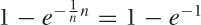 unique visitors (unique data points).)
Class Imbalance Problems
A special case of particular importance concerns situations where one of the classes occurs much less frequently than any of the other classes in the data set—and, as luck would have it, that’s usually the class we are interested in! Consider credit card fraud detection, for instance: only one of every hundred credit card transactions may be fraudulent, but those are exactly the ones we are interested in. Screening lab results for patients with elevated heart attack risk or inspecting manufactured items for defects falls into the same camp: the “interesting” cases are rare, perhaps extremely rare, but those are precisely the cases that we want to identify.
For cases like this, there is some additional terminology as well as some special techniques for overcoming the technical difficulties. Because there is one particular class that is of greater interest, we refer to an instance belonging to this class as a positive event and the class itself as the positive class. With this terminology, entries in the confusion matrix (see Table 18-1) are often referred to as true (or false) positives (or negatives).
I have always found this terminology very confusing, in part because what is called “positive” is usually something bad: a fraudulent transaction, a defective item, a bad heart. Table 18-2 shows a confusion matrix employing the special terminology for problems with a class imbalance—and also an alternative terminology that may be more intuitive.
The two different types of errors may have very different costs associated with them. From the point of view of a merchant accepting credit cards as payment, a false negative (i.e., a fraudulent transaction incorrectly classified as “not fraudulent”—a “miss”) results in the total loss of the item purchased, whereas a false positive (a valid transaction incorrectly classified as “not valid”—a “false alarm”) results only in the loss of the profit margin on that item.
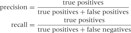
The usual metrics by which we evaluate a classifier (such as accuracy and error rate), may not be very meaningful in situations with pronounced class imbalances: keep in mind that the trivial classifier that labels every credit card transaction as “valid” is 99 percent accurate—and entirely useless! Two metrics that provide better insight into the ability of a classifier to detect instances belonging to the positive class are recall and precision. The precision is the fraction of correct classifications among all instances labeled positive; the recall is the fraction of correct classifications among all instances labeled negative:
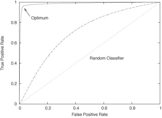
You can see that we will need to strike a balance. On the one hand, we can build a classifier that is very aggressive, labeling many transactions as “bad,” but it will have a high false-positive rate, and therefore low precision. On the other hand, we can build a classifier that is highly selective, marking only those instances that are blatantly fraudulent as “bad,” but it will have a high rate of false negatives and therefore low recall. These two competing goals (to have few false positives and few false negatives) can be summarized in a graph known as a receiver operating characteristic (ROC) curve. (The concept originated in signal processing, where it was used to describe the ability of a receiver to distinguish a true signal from a spurious one in the presence of noise, hence the name.)
Figure 18-6 shows an example of a ROC curve. Along the horizontal axis, we plot the false positive rate (good events that were labeled as bad—“false alarms”) and along the vertical axis we plot the true positive rate (bad events labeled as bad—“hits”). The lower-left corner corresponds to a maximally conservative classifier, which labels every instance as good; the upper-right corner corresponds to a maximally aggressive classifier, which labels everything as bad. We can now imagine tuning the parameters and thresholds of our classifier to shift the balance between “misses” and “false alarms” and thereby mapping out the characteristic curve for our classifier. The curve for a random classifier (which assigns a positive class label with fixed probability p, irrespective of attribute values) will be close to the diagonal: it is equally likely to classify a good instance as good as it is to classify a bad one as good, hence its false positive rate equals its true positive rate. In contrast, the ideal classifier would have a true positive rate equal to 1 throughout. We want to tune our classifier so that it approximates the ideal classifier as nearly as possible.
Class imbalances pose some technical issues during the training phase: if positive instances are extremely rare, then we want to make sure to retain as much of their information as possible in the training set. One way to achieve this is by oversampling (i.e., resampling) from the positive class instances—and undersampling from the negative class instances—when generating a training set.
The Secret Sauce
All this detail about different algorithms and processes can easily leave the impression that that’s all there is to classification. That would be unfortunate, because it leaves out what can be the most important but also the most difficult part of the puzzle: finding the right attributes!
The choice of attributes matters for successful classification—arguably more so than the choice of classification algorithm. Here is an interesting case story. Paul Graham has written two essays on using Bayesian classifiers for spam filtering.[31] In the second one, he describes how using the information contained in the email headers is critical to obtaining good classification results, whereas using only information in the body is not enough. The punch line here is clear: in practice, it matters a lot which features or attributes you choose to include.
Unfortunately, when compared with the extremely detailed information available on different classifier algorithms and their theoretical properties, it is much more difficult to find good guidance regarding how best to choose, prepare, and encode features for classification. (None of the current books on classification discuss this topic at all.)
I think there are several reasons for this relative lack of easily available information—despite the importance of the topic. One of them is lack of rigor: whereas one can prove rigorous theorems on classification algorithms, most recommendations for feature preparation and encoding would necessarily be empirical and heuristic. Furthermore, every problem domain is different, which makes it difficult to come up with recommendations that would be applicable more generally. The implication is that factors such as experience, familiarity with the problem domain, and lots of time-consuming trial and error are essential when choosing attributes for classification. (A last reason for the relative lack of available information on this topic may be that some prefer to keep their cards a little closer to their chest: they may tell you how it works “in theory,” but they won’t reveal all the tricks of the trade necessary to fully replicate the results.)
The difficulty of developing some recommendations that work in general and for a broad range of application domains may also explain one particular observation regarding classification: the apparent scarcity of spectacular, well-publicized successes. Spam filtering seems to be about the only application that clearly works and affects many people directly. Credit card fraud detection and credit scoring are two other widely used (if less directly visible) applications. But beyond those two, I see only a host of smaller, specialized applications. This suggests again that every successful classifier implementation depends strongly on the details of the particular problem—probably more so than on the choice of algorithm.
The Nature of Statistical Learning
Now that we have seen some of the most commonly used algorithms for classification as well as some of the related practical techniques, it’s easy to feel a bit overwhelmed—there seem to be so many different approaches (each nontrivial in its own way) that it can be hard to see the commonalities among them: the “big picture” is easily lost. So let’s step back for a moment and reflect on the specific challenges posed by classification problems and on the overall strategy by which the various algorithms overcome these challenges.
The crucial problem is that from the outset, we don’t have good insight into which features are the most relevant in predicting the class—in fact, we may have no idea at all about the processes (if any!) that link observable features to the resulting class. Because we don’t know ahead of time which features are likely to be most important, we need to retain them all and perhaps even expand the feature set in an attempt to include any possible clue we can get. In this way, the problem quickly becomes very multi-dimensional. That’s the first challenge.
But now we run into a problem: multi-dimensional data sets are invariably sparse data sets. Think of a histogram with (say) 5 bins per dimension. In one dimension, we have 5 bins total. If we want on average at least 5 items per bin, we can make do with 25 items total. Now consider the same data set in two dimensions. If we still require 5 bins per dimension, we have a total of 25 bins, so that each bin contains on average only a single element. But it is in three dimensions that the situation becomes truly dramatic: now there are 125 bins, so we can be sure that the majority of bins will contain no element at all! It gets even worse in higher dimensions. (Mathematically speaking, the problem is that the number of bins grows exponentially with the number of dimensions: Nd, where d is the number of dimensions and N is the number of bins per dimension. No matter what you do, the number of cells is going to grow faster than you can obtain data. This problem is known as the curse of dimensionality.) That’s the second challenge.
It is this combinatorial explosion that drives the need for larger and larger data sets. We have just seen that the the number of possible attribute value combinations grows exponentially; therefore, if we want to have a reasonable chance of finding at least one instance of each possible combination in our training data, we need to have very large data sets indeed. Yet despite our best efforts, we will frequently end up with a sparse data set (as discussed above). Nevertheless, we will often deal with inconveniently large data sets. That’s the third challenge.
Basically all classification algorithms deal with these challenges by using some form of interpolation between points in the sparse data set. In other words, they attempt to smoothly fill the gaps left in the high-dimensional feature space, supported only by a (necessarily sparse) set of points (i.e., the training instances).
Different algorithms do this in different ways: nearest-neighbor methods and naive Bayesian classifiers explicitly “smear out” the training instances to fill the gaps locally, whereas regression and support vector classifiers construct global structures to form a smooth decision boundary from the sparse set of supporting points. Decision trees are similar to nearest-neighbor methods in this regard but provide a particularly fast and efficient lookup of the most relevant neighbors. Their differences aside, all algorithms aim to fill the gaps between the existing data points in some smooth, consistent way.
This brings us to the question of what can actually be predicted in this fashion. Obviously, class labels must depend on attribute values, and they should do so in some smooth, predictable fashion. If the relationship between attribute values and class labels is too crazy, no classifier will be very useful.
Furthermore, the distribution of attribute values for different classes must differ, for otherwise no classifier will be able to distinguish classes by examining the attribute values.
Unfortunately, there is—to my knowledge—no independent, rigorous way of determining whether the information contained in a data set is sufficient to allow the data to be classified. To find out, we must build an actual classifier. If it works, then obviously there is enough information in the data set for classification. But if it does not work, we have learned nothing, because it is always possible that a different or more sophisticated classifier would work. But without an independent test, we can spend an infinite amount of time building and refining classifiers on data sets that contain no useful information. We encountered this kind of difficulty already in Chapter 13 in the context of clustering algorithms, but it strikes me as even more of a problem here. The reason is that classification is by nature predictive (or at least should be), whereas uncertainty of this sort seems more acceptable in an exploratory technique such as clustering.
To make this more clear, suppose we have a large, rich data set: many records with many features. We then arbitrarily assign class labels A and B to the records in the data set. Now, by construction, it is clear that there is no way to predict the labels from the “data”—they are, after all, purely random! However, there is no unambiguous test that will clearly say so. We can calculate the correlation coefficients between each feature (or combination of features) and the class label, we can look at the distribution of feature values and see whether they differ from class to class, and so eventually convince ourselves that we won’t be able to build a good classifier given this data set. But there is no clear test or diagnostic that would give us, for instance, an upper bound on the quality of any classifier that could be built based on this data set. If we are not careful, we may spend a lot of time vainly attempting to build a classifier capable of extracting useful information from this data set. This kind of problem is a trap to be aware of!
Workshop: Two Do-It-Yourself Classifiers
With classification especially, it is really easy to end up with a black-box solution: a tool or library that provides an implementation of a classification algorithm—but one that we would not be able to write ourselves if we had to. This kind of situation always makes me a bit uncomfortable, especially if the algorithms require any parameter tuning to work properly. In order to adjust such parameters intelligently, I need to understand the algorithm well enough that I could at least provide a rough-cut version myself (much as I am happy to rely on the library designer for the high-performance version).
In this spirit, instead of discussing an existing classification library, I want to show you how to write straightforward (you might say “toy version”) implementations for two simple classifiers: a nearest-neighbor lazy learner and a naive Bayesian classifier. (I’ll give some pointers to other libraries near end of the section.)
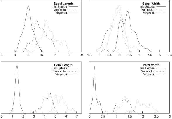
We will test our implementations on the classic data set in all of classification: Fisher’s Iris data set.[32] The data set contains measurements of four different parts of an iris flower (sepal length and width, petal length and width). There are 150 records in the data set, distributed equally among three species of Iris (Iris setosa, versicolor, and virginica). The task is to predict the species based on a given a set of measurements.
First of all, let’s take a quick look at the distributions of the four quantities, to see whether it seems feasible to distinguish the three classes this way. Figure 18-7 shows histograms (actually, kernel density estimates) for all four quantities, separately for the three classes. One of the features (sepal width) does not seem very promising, but the distributions of the other three features seem sufficiently separated that it should be possible to obtain good classification results.
As preparation, I split the original data set into two parts: a
training set (in the file iris.trn)
and a test set (in file iris.tst).
I randomly selected five records from each class for the test set; the
remaining records were used for training. The test set is shown in
full below: the columns are (in order) sepal length, sepal width,
petal length, petal width, and the class label. (All measurements are
in centimeters and to millimeter precision.)
5.0,3.6,1.4,0.2,Iris-setosa
4.8,3.0,1.4,0.1,Iris-setosa
5.2,3.5,1.5,0.2,Iris-setosa
5.1,3.8,1.6,0.2,Iris-setosa
5.3,3.7,1.5,0.2,Iris-setosa
5.7,2.8,4.5,1.3,Iris-versicolor
5.2,2.7,3.9,1.4,Iris-versicolor
6.1,2.9,4.7,1.4,Iris-versicolor
6.1,2.8,4.7,1.2,Iris-versicolor
6.0,3.4,4.5,1.6,Iris-versicolor
6.3,2.9,5.6,1.8,Iris-virginica
6.2,2.8,4.8,1.8,Iris-virginica
7.9,3.8,6.4,2.0,Iris-virginica
5.8,2.7,5.1,1.9,Iris-virginica
6.5,3.0,5.2,2.0,Iris-virginica
Our implementation of the nearest-neighbor classifier is shown in the next listing. The implementation is exceedingly simple—especially once you realize that about two thirds of the listing deal with file input and output. The actual “classification” is a matter of three lines in the middle:
# A Nearest-Neighbor Classifier

from numpy import *

train = loadtxt( "iris.trn", delimiter=',', usecols=(0,1,2,3) )
trainlabel = loadtxt( "iris.trn", delimiter=',', usecols=(4,), dtype=str )

test = loadtxt( "iris.tst", delimiter=',', usecols=(0,1,2,3) )
testlabel = loadtxt( "iris.tst", delimiter=',', usecols=(4,), dtype=str )

hit, miss = 0, 0
for i in range( test.shape[0] ):
    dist = sqrt( sum( (test[i] - train)**2, axis=1 ) )
    k = argmin( dist )

    if trainlabel[k] == testlabel[i]:
        flag = '+'
        hit += 1
    else:
        flag = '-'
        miss += 1

    print flag, "\t Predicted: ", trainlabel[k], "\t True: ", testlabel[i]

print
print hit, "out of", hit+miss, "correct - Accuracy: ", hit/(hit+miss+0.0)
The algorithm loads both the training and the test data set into two-dimensional NumPy arrays. Because all elements in a NumPy array must be of the same type, we store the class labels (which are strings, not numbers) in separate vectors.
Now follows the actual classification step: for each element of
the test set, we calculate the Euclidean distance to each element in
the training set. We make use of NumPy “broadcasting” (see the
Workshop in Chapter 2) to calculate
the distance of the test instance test[i] from all
training instances in one fell swoop. (The argument axis=1 is necessary to tell NumPy that the
sum in the Euclidean distance should be taken over the
inner (horizontal) dimension of the
two-dimensional array.) Next, we use the argmin() function to obtain the index of the
training record that has the smallest distance to the current test
record: this is our predicted class label. (Notice that we base our
result only on a single record—namely the closest training
instance.)
Simple as it is, the classifier works very well (on this data set). For the test set shown, all records in the test set are classified correctly!
The naive Bayesian classifier implementation is next. A naive
Bayesian classifier needs an estimate of the probability distribution
P(class C | feature
x), which we find from a histogram of attribute
values, separately for each class. In this case, we need a total of 12
histograms (3 classes × 4 features). I maintain this data in a triply
nested data structure: histo[label][feature][value]. The first
index is the class label, the second index specifies the feature, and
the third contains the values of the feature that occur in the
histogram. The value stored in the histogram is the number of times
that each value has been observed:
# A Naive Bayesian Classifier

total = {}  # Training instances per class label
histo = {}  # Histogram

# Read the training set and build up a histogram
train = open( "iris.trn" )
for line in train:
    # seplen, sepwid, petlen, petwid, label
    f = line.rstrip().split( ',' )
    label = f.pop()

    if not total.has_key( label ):
        total[ label ] = 0
        histo[ label ] = [ {},  {},  {},  {} ]

    # Count training instances for the current label
    total[label] += 1

    # Iterate over features
    for i in range( 4 ):
        histo[label][i][f[i]]  = 1 + histo[label][i].get( f[i], 0.0 )

train.close()

# Read the test set and evaluate the probabilities
hit, miss = 0, 0
test = open( "iris.tst" )
for line in test:
    f = line.rstrip().split( ',' )
    true = f.pop()

    p = {}  # Probability for class label, given the test features
    for label in total.keys():
        p[label] = 1
        for i in range( 4 ):
            p[label] *= histo[label][i].get(f[i],0.0)/total[label]

    # Find the label with the largest probability
    mx, predicted = 0, -1
    for k in p.keys():
        if p[k] >= mx:
            mx, predicted = p[k], k

    if true == predicted:
        flag = '+'
        hit += 1

    else:
        flag = '-'
        miss += 1

    print flag, "\t", true, "\t", predicted, "\t",
    for label in p.keys():
        print label, ":", p[label], "\t",
    print

print
print hit, "out of", hit+miss, "correct - Accuracy: ", hit/(hit+miss+0.0)

test.close()
I’d like to point out two implementation details. The first is that the second index is an integer, which I use instead of the feature names; this simplifies some of the loops in the program. The second detail is more important: I know that the feature values are given in centimeters, with exactly one digit after the decimal point. In other words, the values are already discretized, and so I don’t need to “bin” them any further—in effect, each bin in the histogram is one millimeter wide. Because I never need to operate on the feature values, I don’t even convert them to numbers: I read them as strings from file and use them (as strings) as keys in the histogram. Of course, if we wanted to use a different bin width, then we would have to convert them into numerical values so that we can operate on them.
In the evaluation part, the program reads data points from the test set and then evaluates the probability that the record belongs to a certain class for all three class labels. We then pick the class label that has the highest probability. (Notice that we don’t need an explicit factor for the prior probability, since we know that each class is equally likely.)
On the test set shown earlier, the Bayesian classifier does a little worse than the nearest neighbor classifier: it correctly classifies 12 of 15 instances for a total accuracy of 80 percent.
If you look at the results of the classifier more closely, you will immediately notice a couple of problems that are common with Bayesian classifiers. First of all, the posterior probabilities are small. This should come as no surprise: each Bayes factor is smaller than 1 (because it’s a probability), so their product becomes very small very quickly. To avoid underflows, it’s usually a good idea to add the logarithms of the probabilities instead of multiplying the probabilities directly. In fact, if you have a greater number of features, this becomes a necessity. The second problem is that many of the posterior probabilities come out as exactly zero: this occurs whenever no entry in the histogram can be found for at least one of the feature values in the test record; in this case the histogram evaluates to zero, which means the entire product of probabilities is also identical to zero. There are different ways of dealing with this problem—in our case, you might want to experiment with replacing the histogram of discrete feature values with a kernel density estimate (similar to those in Figure 18-7), which, by construction, is nonzero everywhere. Keep in mind that you will need to determine a suitable bandwidth for each histogram!
Let me be clear: the implementations of both classifiers are extremely simpleminded. My intention here is to demonstrate the basic ideas behind these algorithms in as few lines of code as possible—and also to show that there is nothing mystical about writing a simple classifier. Because the implementations are so simple, it is easy to continue experimenting with them: can we do better if we use a larger number of neighbors in our nearest-neighbor classifier? How about a different distance function? In the naive Bayesian classifier, we can experiment with different bin widths in the histogram or, better yet, replace the histogram of discrete bins with a kernel density estimate. In either case, we need to start thinking about runtime efficiency: for a data set of only 150 elements this does not matter much, but evaluating a kernel density estimate of a few thousand points can be quite expensive!
If you want to use an established tool or library, there are several choices in the open source world. Three projects have put together entire data analysis and mining “toolboxes,” complete with graphical user interface, plotting capabilities, and various plug-ins: RapidMiner (http://rapid-i.com/) and WEKA (http://www.cs.waikato.ac.nz/ml/weka/), which are both in Java as well as Orange (http://www.ailab.si/orange/), which is in Python. WEKA has been around for a long time and is very well established; RapidMiner is part of a more comprehensive tool suite (and includes WEKA as a plug-in). Orange is an alternative using Python.
All three of these projects use a “pipeline” metaphor: you select different processing steps (discretizers, smoothers, principal component analysis, regression, classifiers) from a toolbox and string them together to build up the whole analysis workflow entirely within the tool. Give it a shot—the idea has a lot of appeal, but I must confess that I have never succeeded in doing anything nontrivial with any of them!
There are some additional libraries worth checking out that have Python interfaces: libSVM (http://www.csie.ntu.edu.tw/~cjlin/libsvm/) and Shogun (http://www.shogun-toolbox.org/) provide implementations of support vector machines, while the Modular toolkit for Data Processing (http://mdp-toolkit.sourceforge.net/) is more general. (The latter also adheres to the “pipeline” metaphor.)
Finally, all classification algorithms are also available as R
packages. I’ll mention just three: the class package for nearest-neighbor
classifiers and the rpart package
for decision trees (both part of the R standard distribution) as well
as the e1071 package (which can be
found on CRAN) for support vector machines and naive Bayesian
classifiers.
Further Reading
Introduction to Data Mining. Pang-Ning Tan, Michael Steinbach, and Vipin Kumar. Addison-Wesley. 2005.
This is my favorite book on data mining. It contains two accessible chapters on classification.
The Elements of Statistical Learning. Trevor Hastie, Robert Tibshirani, and Jerome Friedman. 2nd ed., Springer. 2009.
This book exemplifies some of the problems with current machine-learning theory: an entire book of highly nontrivial mathematics—and what feels like not a single real-world example or discussion of “what to use when.”
[30] The techniques discussed in Part III are different: for the most part they were strictly computational and can be applied to any purpose, depending on the context.
[31] “A Plan for Spam” (http://www.paulgraham.com/spam.html) and “Better Bayesian Filtering” (http://www.paulgraham.com/better.html).
[32] First published in 1936. The data set is available from many sources, for example in the “Iris” data set on the UCI Machine Learning repository at http://archive.ics.uci.edu/ml/.