Table of Contents for
Data Analysis with Open Source Tools
 Data Analysis with Open Source Tools
Published by
O'Reilly Media, Inc., 2010
Data Analysis with Open Source Tools
Published by
O'Reilly Media, Inc., 2010
- Cover
- Data Analysis with Open Source Tools
- O'Reilly Strata Conference
- Data Analysis with Open Source Tools
- Dedication
- A Note Regarding Supplemental Files
- Preface
- 1. Introduction
- I. Graphics: Looking at Data
- 2. A Single Variable: Shape and Distribution
- 3. Two Variables: Establishing Relationships
- 4. Time As a Variable: Time-Series Analysis
- 5. More Than Two Variables: Graphical Multivariate Analysis
- 6. Intermezzo: A Data Analysis Session
- II. Analytics: Modeling Data
- 7. Guesstimation and the Back of the Envelope
- 8. Models from Scaling Arguments
- 9. Arguments from Probability Models
- 10. What You Really Need to Know About Classical Statistics
- 11. Intermezzo: Mythbusting—Bigfoot, Least Squares, and All That
- III. Computation: Mining Data
- 12. Simulations
- 13. Finding Clusters
- 14. Seeing the Forest for the Trees: Finding Important Attributes
- 15. Intermezzo: When More Is Different
- IV. Applications: Using Data
- 16. Reporting, Business Intelligence, and Dashboards
- 17. Financial Calculations and Modeling
- 18. Predictive Analytics
- 19. Epilogue: Facts Are Not Reality
- A. Programming Environments for Scientific Computation and Data Analysis
- B. Results from Calculus
- C. Working with Data
- D. About the Author
- Index
- About the Author
- Colophon
- Copyright
Chapter 8. Models from Scaling Arguments
AFTER FAMILIARIZING YOURSELF WITH THE DATA THROUGH PLOTS AND GRAPHS, THE NEXT STEP IS TO START building a model for the data. The meaning of the word “model” is quite hazy, and I don’t want to spend much time and effort attempting to define this concept in an abstract way. For our purposes, a model is a mathematical description of the data that ideally is guided by our understanding of the system under consideration and that relates the various variables of the system to each other: a “formula.”
Models
Models like this are incredibly important. It is at this point that we go from the merely descriptive (plots and graphs) to the prescriptive: having a model allows us to predict what the system will do under a certain set of conditions. Furthermore, a good or truly useful model—because it helps us to understand how the system works—allows us to do so without resorting to the model itself or having to evaluate any particular formula explicitly. A good model ties the different variables that control the system together in such a way that we can see how varying any one of them will influence the outcome. It is this use of models—as an aide to or expression of our understanding—that is the most important one. (Of course, we must still evaluate the model formulas explicitly in order to obtain actual numbers for a specific prediction.)
I should point out that this view of models and what they can do is not universal, and you will find the term used quite differently elsewhere. For instance, statistical models (and this includes machine-learning models) are much more descriptive: they do not purport to explain the observed behavior in the way just described. Instead, their purpose is to predict expected outcomes with the greatest level of accuracy possible (numbers in, numbers out). In contrast, my training is in theoretical physics, where the development of conceptual understanding of the observed behavior is the ultimate goal. I will use all available information about the system and how it works (or how I suspect it works!) wherever I can; I don’t restrict myself to using only the information contained in the data itself. (This is a practice that statisticians traditionally frown upon, because it constitutes a form of “pollution” of the data. They may very well be right, but my purpose is different: I don’t want to understand the data, I want to understand the system!) At the same time, I don’t consider the absolute accuracy of a model paramount: a model that yields only order-of-magnitude accuracy but helps me understand the system’s behavior (so that I can, for instance, make informed trade-off decisions) is much more valuable to me than a model that yields results with 1 percent accuracy but that is a black box otherwise.
To be clear: there are situations when achieving the best possible accuracy is all that matters and conceptual understanding is of little interest. (Often these cases involve repeatable processes in well-understood systems.) If this describes your situation, then you need to use different methods that are appropriate to your problem scenario.
Modeling
As should be clear from the preceding description, building models is basically a creative process. As such, it is difficult (if not impossible) to teach: there are no established techniques or processes for arriving at a useful model in any given scenario. One common approach to teaching this material is to present a large number of case studies, describing the problem situations and attempts at modeling them. I have not found this style to be very effective. First of all, every (nontrivial) problem is different, and tricks and fortuitous insights that work well for one example rarely carry over to a different problem. Second, building effective models often requires fairly deep insight into the particulars of the problem space, so you may end up describing lots of tedious details of the problem when actually you wanted to talk about the model (or the modeling).
In this chapter, we will take a different approach. Effective modeling is often an exercise in determining “what to leave out”: good models should be simple (so that they are workable) yet retain the essential features of the system—certainly those that we are interested in.
As it turns out, there are a few essential arguments and approximations that prove helpful again and again to make a complex problem tractable and to identify the dominant behavior. That’s what I want to talk about.
Using and Misusing Models
Just a reminder: models are not reality. They are descriptions or approximations of reality—often quite coarse ones! We need to ensure that we only place as much confidence in a model as is warranted.
How much confidence is warranted? That depends on how well-tested the model is. If a model is based on a good theory, agrees well with a wide range of data sets, and has shown it can predict observations correctly, then our confidence may be quite strong.
At the other extreme are what one might call “pie in the sky” models: ad hoc models, involving half a dozen (or so) parameters—all of which have been estimated independently and not verified against real data. The reliability of such a model is highly dubious: each of the parameters introduces a certain degree of uncertainty, which in combination can make the results of the model meaningless. Recall the discussion in Chapter 7: three parameters known to within 10 percent produce an uncertainty in the final result of 30 percent—and that assumes that the parameters are actually known to within 10 percent! With four to six parameters that possibly are known, only much less precisely than 10 percent, the situation is correspondingly worse. (Many business models fall into this category.)
Also keep in mind that virtually all models have only a limited region of validity. If you try to apply an existing model to a drastically different situation or use input values that are very different from those that you used to build the model, then you may well find that the model makes poor predictions. Be sure to check that the assumptions on which the model is based are actually fulfilled for each application that you have in mind!
Arguments from Scale
Next to the local stadium there is a large, open parking lot. During game days, the parking lot is filled with cars, and—for obvious reasons—a line of portable toilets is set up all along one of the edges of the parking lot. This poses an interesting balancing problem: will this particular arrangement work for all situations, no matter how large the parking lot in question?
The answer is no. The number of people in the parking lot grows with the area of the parking lot, which grows with the square of the edge length (i.e., it “scales as” L2); but the number of toilets is proportional to the edge length itself (so it scales as L). Therefore, as we make the parking lot bigger and bigger, there comes a point where the number of people overwhelms the number of available facilities. Guaranteed.
Scaling Arguments
This kind of reasoning is an example of a scaling argument. Scaling arguments try to capture how some quantity of interest depends on a control parameter. In particular, a scaling argument describes how the output quantity will change as the control parameter changes. Scaling arguments are a particularly fruitful way to arrive at symbolic expressions for phenomena (“formulas”) that can be manipulated analytically.
You should have observed that the expressions I gave in the introductory example were not “dimensionally consistent.” We had people expressed as the square of a length and toilets expressed as length—what is going on here? Nothing, I merely omitted some detail that was not relevant for the argument I tried to make. A car takes up some amount of space on a parking lot; hence given the size of the parking lot (its area), we can figure out how many cars it can accommodate. Each car seats on average two people (on a game day), so we can figure out the number of people as well. Each person has a certain probability of using a bathroom during the duration of the game and will spend a certain number of minutes there. Given all these parameters, we can figure out the required “toilet availability minutes.” We can make a similar argument to find the “availability minutes” provided by the installed facilities. Observe that none of these parameters depend on the size of the parking lot: they are constants. Therefore, we don’t need to worry about them if all we want to determine is whether this particular arrangement (with toilets all along one edge, but nowhere else) will work for parking lots of any size. (It is a widely followed convention to use the tilde, as in A ~ B, to express that A “scales as” B, where A and B do not necessarily have the same dimensions.)
On the other hand, if we actually want to know the exact number of toilets required for a specific parking lot size, then we do need to worry about these factors and try to obtain the best possible estimates for them.
Because scaling arguments free us from having to think about pesky numerical factors, they provide such a convenient and powerful way to begin the modeling process. At the beginning, when things are most uncertain and our understanding of the system is least developed, they free us from having to worry about low-level details (e.g., how long does the average person spend in the bathroom?) and instead help us concentrate on the system’s overall behavior. Once the big picture has become clearer (and if the model still seems worth pursuing), we may want to derive some actual numbers from it as well. Only at this point do we need to concern ourselves with numerical constants, which we must either estimate or derive from available data.
A recurring challenge with scaling models is to find the correct scales. For example, we implicitly assumed that the parking lot was square (or at least nearly so) and would remain that shape as it grew. But if the parking lot were growing in one direction only (i.e., becoming longer and longer, while staying the same width), then its area would no longer scale as L2 but instead scale as L, where L is now the “long” side of the lot. This changes the argument, for if the portable toilets were located along the long side of the lot then the balance between people and available facilities would be the same no matter how large the lot became! On the other hand, if the facilities were set up along the short side, then their number would remain constant while the long side grew, resulting again in an imbalanced situation.
Finding the correct scales is a bit of an experience issue—the important point here is that it is not as simple as saying: “It’s an area, therefore it must scale as length squared.” It depends on the shape of the area and on which of its lengths controls the size.
The parking lot example demonstrates one typical application of high-level scaling arguments: what I call a “no-go argument.” Even without any specific numbers, the scaling behavior alone was enough to determine that this particular arrangement of toilets to visitors will break down at some point.
Example: A Dimensional Argument
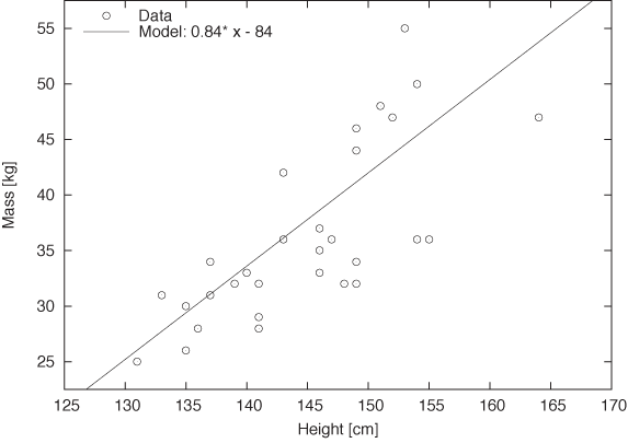
Figure 8-1 shows the heights and weights of a class of female middle-school students.[15] Also displayed is the function m = 0.84h – 84.0, where m stands for the mass (or weight) and h for the height. The fit seems to be quite close—is this a good model?
The answer is no, because the model makes unreasonable predictions. Look at it: the model suggests that students have no weight unless they are at least 84 centimeters (almost 3 feet) tall; if they were shorter, their weight would be negative. Clearly, this model is no good (although it does describe the data over the range shown quite well). We expect that people who have no height also have no weight, and our model should reflect that.
Rather than a model of the form ax + b, we might instead try axb, because this is the simplest function that gives the expected result for x = 0.
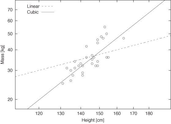
Figure 8-2 shows the same data but on a double logarithmic plot. Also indicated are functions of the form y = ax and y = ax3. The cubic function ax3 seems to represent the data quite well—certainly better than the linear function.
But this makes utmost sense! The weight of a body is proportional to its volume—that is, to height times width times depth or h · w · d. Since body proportions are pretty much the same for all humans (i.e., a person who is twice as tall as another will have shoulders that are twice as wide, too), it follows that the volume of a person’s body (and hence its mass) scales as the third power of the height: mass ~ height3.
Figure 8-3 shows the data one more time and together with the model m = 1.25 · 10–5h3. Notice that the model makes reasonable predictions even for values outside the range of available data points, as you can see by comparing the model predictions with the average body measurements for some different age groups. (The figure also shows the possible limitations of a model that is built using less than perfectly representative data: the model underestimates adult weights because middle-school students are relatively light for their size. In contrast, two-year-olds are notoriously “chubby.”)
Nevertheless, this is a very successful model. On the one hand, although based on very little data, the model successfully predicts the weight to within 20 percent accuracy over a range of almost two orders of magnitude in height. On the other hand, and arguably more importantly, it captures the general relationship between body height and weight—a relationship that makes sense but that we might not necessarily have guessed without looking at the data.
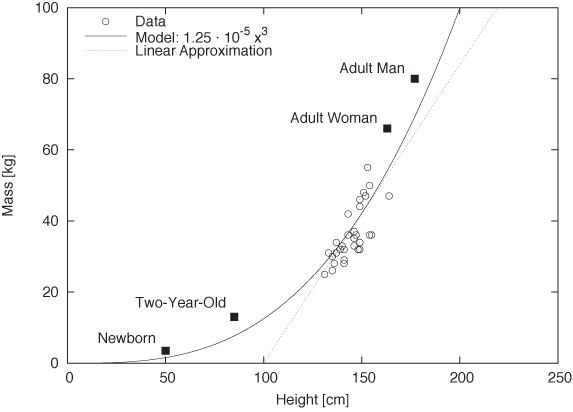
The last question you may ask is why the initial description, m = 0.84x – 84 in Figure 8-1 seemed so good. The answer is that this is exactly the linear approximation to the correct model, m = 1.25 · 10–5h3, near h = 150 cm. (See Appendix B.) As with all linear approximations, it works well in a small region but fails for values farther away.
Example: An Optimization Problem
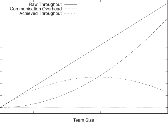
Another application of scaling arguments is to cast a question as an optimization problem. Consider a group of people scheduled to perform some task (say, a programming team). The amount of work that this group can perform in a fixed amount of time (its “throughput”) is obviously proportional to the number n of people on the team: ~ n. However, the members of the team will have to coordinate with each other. Let’s assume that each member of the team needs to talk to every other member of the team at least once a day. This implies a communication overhead that scales the square of the number of people: ~ –n2. (The minus sign indicates that the communication overhead results in a loss in throughput.) This argument alone is enough to show that for this task, there is an optimal number of people for which the realized productivity will be highest. (Also see Figure 8-4.)
To find the optimal staffing level, we want to maximize the productivity P with respect to the number of workers on the team n:
P(n) = cn – dn2
where c is the number of minutes each person can contribute during a regular workday, and d is the effective number of minutes consumed by each communication event. (I’ll return to the cautious “effective” modifier shortly.)
To find the maximum, we take the derivative of P(n) with respect to n, set it equal to 0, and solve for n (see Appendix B). The result is:
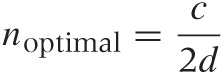
Clearly, as the time consumed by each communication event d grows larger, the optimal team size shrinks.
If we now wish to find an actual number for the optimal staffing level, then we need to worry about the numerical factors, and this is where the “effective” comes in. The total number of hours each person can put in during a regular workday is easy to estimate (8 hours at 60 minutes, less time for diversions), but the amount of time spent in a single communication event is more difficult to determine. There are also additional effects that I would lump into the “effective” parameter: for example, not everybody on the team needs to talk to everybody else. Adjustments like this can be lumped into the parameter d which increasingly turns it into a synthetic parameter and less one that can be measured directly.
Example: A Cost Model
Models don’t have to be particularly complicated to provide important insights. I remember a situation where we were trying to improve the operation of a manufacturing environment. One particular job was performed on a special machine that had to be retooled for each different type of item to be produced. First the machine would be set up (which took about 5 to 10 minutes), and then a worker would operate the machine to produce a batch of 150 to 200 identical items. The whole cycle lasted a bit longer than an hour and a half to complete the batch, and then the machine was retooled for the next batch.
The retooling part of the cycle was a constant source of management frustration: for 10 minutes (while the machine was being set up), nothing seemed to be happening. Wasted time! (In manufacturing, productivity—defined as “units per hour”—is the most closely watched metric.) Consequently, there had been a long string of process improvement projects dedicated to making the retooling part more efficient and thereby faster. By the time I arrived, it had been streamlined very well. Nevertheless, there were constant efforts underway to reduce the time it took—after all, the sight of the machine sitting idle for 10 minutes seemed to be all the proof that was needed.
It is interesting to set up a minimal cost model for this process. The relevant quantity to study is “minutes per unit.” This is essentially the inverse of the productivity, but I find it easier to think in terms of the time it takes to produce a single unit than the other way around. Also note that “time per unit” equates to “cost per unit” after we take the hourly wage into account. Thus, the time per unit is the time T it takes to produce an entire batch, divided by the number of items n in the batch. The total processing time itself consists of the setup time T1 and n times the amount of time t required to produce a single item:
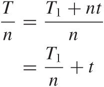
The first term on the righthand side is the amount of the setup time that can be attributed to a single item; the second term, of course, is the time it takes to actually produce the item. The larger the batch size, the smaller the contribution of the setup time to the cost of each item as the setup time is “amortized” over more units.
This is one of those situations where the numerical factors actually matter. We know that T1 is in the range of 300–600 seconds, and that n is between 150 and 200, so that the setup time per item, T1/n, is between 1–4 seconds. We can also find the time t required to actually produce a single item if we recall that the cycle time for the entire batch was about 90 minutes; therefore t = 90 · 60/n, which is about 30 seconds per item. In other words, the setup time that caused management so much grief actually accounted for less than 10 percent of the total time to produce an item!
But we aren’t finished yet. Let’s assume that, through some strenuous effort, we are able to reduce the setup time by 10 percent. (Not very likely, given that this part of the process had already received a lot of attention, but let’s assume—best case!) This would mean that we can reduce the setup time per item to 1–3.5 seconds. However, this means that the total time per item is reduced by only 1 or 2 percent! This is the kind of efficiency gain that makes sense only in very, very controlled situations where everything else is completely optimized. In contrast, a 10 percent reduction in t, the actual work time per item, would result in (almost) a 10 percent improvement in overall productivity (because the amount of time that it takes to produce an item is so much greater than the fraction of the setup time attributable to a single item).
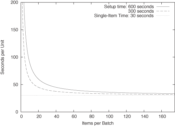
We can see this in Figure 8-5 which shows the “loaded” time per unit (including the setup time) for two typical values of the setup time as a function of the number of items produced in a single batch. Although the setup time contributes significantly to the per-item time when there are fewer than about 50 items per batch, its effect is very small for batch sizes of 150 or more. For batches of this size, the time it takes to actually make an item dominates the time to retool the machine.
The story is still not finished. We eventually launched a project to look at ways to reduce t for a change, but it was never strongly supported and shut down at the earliest possible moment by plant management in favor of a project to look at, you guessed it, the setup time! The sight of the machine sitting idle for 10 minutes was more than any self-respecting plant manager could bear.
Optional: Scaling Arguments Versus Dimensional Analysis
Scaling arguments may seem similar to another concept you may have heard of: dimensional analysis. Although they are related, they are really quite different. Scaling concepts, as introduced here, are based on our intuition of how the system behaves and are a way to capture this intuition in a mathematical expression.
Dimensional analysis, in contrast, applies to physical systems, which are described by a number of quantities that have different physical dimensions, such as length, mass, time, or temperature. Because equations describing a physical system must be dimensionally consistent, we can try to deduce the form of these equations by forming dimensionally consistent combinations of the relevant variables.
Let’s look at an example. Everybody is familiar with the phenomenon of air resistance, or drag: there is a force F that acts to slow a moving body down. It seems reasonable to assume that this force depends on the cross-sectional area of the body A and the speed (or velocity) ν. But it must also depend on some property of the medium (air, in this case) through which the body moves. The most basic property is the density ρ, which is the mass (in grams or kilograms) per volume (in cubic centimeters or meters):
F = f(A, υ, ρ)
Here, f(x, y, z) is an as-yet-unknown function.
Force has units of mass · length/time2, area has units of length2, velocity of length/time, and density has units of mass/length3. We can now try to combine A, υ, and ρ to form a combination that has the same dimensions as force. A little experimentation leads us to:
F = cρ Aυ2
where c is a pure (dimensionless) number. This equation expresses the well-known result that air resistance increases with the square of the speed. Note that we arrived at it using purely dimensional arguments without any insight into the physical mechanisms at work.
This form of reasoning has a certain kind of magic to it: why
did we choose these specific quantities? Why did we not include the
viscosity of air, the ambient air pressure, the temperature, or the
length of the body? The answer is (mostly) physical intuition. The
viscosity of air is small (viscosity measures the resistance to
shear stress, which is the force transmitted by a fluid captured
between parallel plates moving parallel to each other but in
opposite directions—clearly, not a large effect for air at
macroscopic length scales). The pressure enters indirectly through
the density (at constant temperature, according to the ideal gas
law). And the length of the body is hidden in the numerical factor
c, which depends on the shape of the body and
therefore on the ratio of the cross-sectional radius
 to the length. In summary: it is impressive
how far we came using only very simple arguments, but it is hard to
overcome a certain level of discomfort entirely.
to the length. In summary: it is impressive
how far we came using only very simple arguments, but it is hard to
overcome a certain level of discomfort entirely.
Methods of dimensional analysis appear less arbitrary when the governing equations are known. If this is the case, then we can use dimensional arguments to reduce the number of independently variable quantities. For example: assume that we already know the drag force is described by F = cρ Aυ2. Suppose further that we want to perform experiments to determine c for various bodies by measuring the drag force on them under various conditions. Naively, it might appear as if we had to map out the full three-dimensional parameter space by making measurements for all combinations of (ρ, A, υ). But these three parameters only occur in the combination γ = ρAυ2, therefore it is sufficient to run a single series of tests that varies γ over the range of values that we are interested in. This constitutes a significant simplification!
Dimensional analysis relies on dimensional consistency and therefore works best for physical and engineering systems, which are described by independently measurable, dimensional quantities. It is particularly prevalent in areas such as fluid dynamics, where the number of variables is especially high, and the physical laws are complicated and often not well understood. It is much less applicable in economic or social settings, where there are fewer (if any) rigorously established, dimensionally consistent relationships.
Other Arguments
There are other arguments that can be useful when attempting to formulate models. They come from the physical sciences, and (like dimensional analysis) they may not work as well in social and economic settings, which are not governed by strict physical laws.
Conservation laws
Conservation laws tell us that some quantity does not change over time. The best-known example is the law of conservation of energy. Conservation laws can be very powerful (in particular when they are exact, as opposed to only approximate) but may not be available: after all, the entire idea of economic growth and (up to a point) manufacturing itself rest on the assumption that more comes out than is being put in!
Symmetries
Symmetries, too, can be helpful in reducing complexity. For example, if an apparently two-dimensional system exhibits the symmetry of a circle, then I know that I’m dealing with a one-dimensional problem: any variation can occur only in the radial direction, since a circle looks the same in all directions. When looking for symmetries, don’t restrict yourself to geometric considerations—for instance, items entering and leaving a buffer at the same rate exhibit a form of symmetry. In this case, you might only need to solve one of the two processes explicitly while treating the other as a mirror image of the first.
Extreme-value considerations
How does the system behave at the extremes? If there are no customers, messages, orders, or items? If there are infinitely many? What if the items are extremely large or vanishingly small, or if we wait an infinite amount of time? Such considerations can help to “sanity check” an existing model, but they can also provide inspiration when first establishing a model. Limiting cases are often easier to treat because only one effect dominates, which eliminates the complexities arising out of the interplay of different factors.
Mean-Field Approximations
The term mean-field approximation comes from statistical physics, but I use it only as a convenient and intuitive expression for a much more general approximation scheme.
Statistical physics deals with large systems of interacting particles, such as gas molecules in a piston or atoms on a crystal lattice. These systems are extraordinarily complicated because every particle interacts with every other particle. If you move one of the particles, then this will affect all the other particles, and so they will move, too; but their movement will, in turn, influence the first particle that we started with! Finding exact solutions for such large, coupled systems is often impossible. To make progress, we ignore the individual interactions between explicit pairs of particles. Instead, we assume that the test particle experiences a field, the “mean-field,” that captures the “average” effect of all the other particles.
For example, consider N gas atoms in a bottle of volume V. We may be interested to understand how often two gas atoms collide with each other. To calculate that number exactly, we would have to follow every single atom over time to see whether it bumps into any of the other atoms. This is obviously very difficult, and it certainly seems as if we would need to keep track of a whole lot of detail that should be unnecessary if we are only interested in macroscopic properties.
Realizing this, we can consider this gas in a mean-field approximation: the probability that our test particle collides with another particle should be proportional to the average density of particles in that bottle ρ = N/V. Since there are N particles in the bottle, we expect that the number of collisions (over some time frame) will be proportional to Nρ. This is good enough to start making some predictions—for example, note that this expression is proportional to N2. Doubling the number of particles in the bottle therefore means that the number of collisions will grow by a factor of 4. In contrast, reducing the volume of the container by half will increase the number of collisions only by a factor of 2.
You will have noticed that in the previous argument, I omitted lots of detail—for example, any reference to the time frame over which I intend to count collisions. There is also a constant of proportionality missing: Nρ is not really the number of collisions but is merely proportional to it. But if all I care about is understanding how the number of collisions depends on the two variables I consider explicitly (i.e., on N and V), then I don’t need to worry about any of these details. The argument so far is sufficient to work out how the number of collisions scales with both N and V.
You can see how mean-field approximations and scaling arguments enhance and support each other. Let’s step back and look at the concept behind mean-field approximations more closely.
Background and Further Examples
If mean-field approximations were limited to systems of interacting particles, they would not be of much interest in this book. However, the concept behind them is much more general and is very widely applicable.
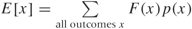
Whenever we want to calculate with a quantity whose values are distributed according to some probability distribution, we face the challenge that this quantity does not have a single, fixed value. Instead, it has a whole spectrum of possible values, each more or less likely according to the probability distribution. Operating with such a quantity is difficult because at least in principle we have to perform all calculations for each possible outcome and then weight the result of our calculation by the appropriate probability. At the very end of the calculation, we eventually form the average (properly weighted according to the probability factors) to arrive at a unique numerical value.
Given the combinatorial explosion of possible outcomes, attempting to perform such a calculation exactly invariably starts to feel like wading in a quagmire—and that assumes that the calculation can be carried out exactly at all!
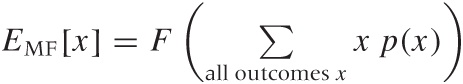
The mean-field approach cuts through this difficulty by performing the average before embarking on the actual calculation. Rather than working with all possible outcomes (and averaging them at the end), we determine the average outcome first and then only work with that value alone. Table 8-1 summarizes the differences.
This may sound formidable, but it is actually something we do all the time. Do you ever try to estimate how high the bill is going to be when you are waiting in line at the supermarket? You can do this explicitly—by going through all the items individually and adding up their prices (approximately) in your head—or you can apply a mean-field approximation by realizing that the items in your cart represent a sample, drawn “at random,” from the selection of goods available. In the mean-field approximation, you would estimate the average single-item price for goods from that store (probably about $5–$7) and then multiply that value by the number of items in your cart. Note that it should be much easier to count the items in your cart than to add up their individual prices explicitly.
This example also highlights the potential pitfalls with mean-field arguments: it will only be reliable if the average item price is a good estimator. If your cart contains two bottles of champagne and a rib roast for a party of eight, then an estimate based on a typical item price of $7 is going to be way off.
To get a grip on the expected accuracy of a mean-field approximation, we can try to find a measure for the width of the original distribution (e.g., its standard deviation or inter-quartile range) and then repeat our calculations after adding (and subtracting) the width from the mean value. (We may also treat the width as a small perturbation to the average value and use the perturbation methods discussed in Chapter 7.)
Another example: how many packages does UPS (or any comparable freight carrier) fit onto a truck (to be clear: I don’t mean a delivery truck, but one of these 53 feet tractor-trailer long-hauls)? Well, we can estimate the “typical” size of a package as about a cubic foot (0.33 m3), but it might also be as small as half that or as large as twice that size. To find an estimate for the number of packages that will fit, we divide the volume of the truck (17 m long, 2 m wide, 2.5 m high—we can estimate height and width if we realize that a person can stand upright in these things) by the typical size of a package: (17 · 2 · 2.5/0.33) ≈ 3,000 packages. Because the volume (not the length!) of each package might vary by as much as a factor of 2, we end up with lower and upper bounds of (respectively) 1,500 to 6,000 packages.
This calculation makes use of the mean-field idea twice. First, we work with the “average” package size. Second, we don’t worry about the actual spatial packing of boxes inside the truck; instead, we pretend that we can reshape them like putty. (This also is a form of “mean-field” approximation.)
I hope you appreciate how the mean-field idea has turned this problem from almost impossibly difficult to trivial—and I don’t just mean with regard to the actual computation and the eventual numerical result; but more importantly in the way we thought about it. Rather than getting stuck in the enormous technical difficulties of working out different stacking orders for packages of different sizes, the mean-field notion reduced the problem description to the most fundamental question: into how many small pieces can we divide a large volume? (And if you think that all of this is rather trivial, I fully agree with you—but the “trivial” can easily be overlooked when one is presented with a complex problem in all of its ugly detail. Trying to find mean-field descriptions helps strip away nonessential detail and helps reveal the fundamental questions at stake.)
One common feature of mean-field solutions is that they frequently violate some of the system’s properties. For example, at Amazon, we would often consider the typical order to contain 1.7 items, of which 0.9 were books, 0.3 were CDs, and the remaining 0.5 items were other stuff (or whatever the numbers were). This is obviously nonsense, but don’t let this disturb you! Just carry on as if nothing happened, and work out the correct breakdown of things at the end. This approach doesn’t always work: you’ll still have to assign a whole person to a job, even it requires only one tenth of a full-time worker. However, this kind of argument is often sufficient to work out the general behavior of things.
There is a story involving Richard Feynman working on the Connection Machine, one of the earliest massively parallel supercomputers. All the other people on the team were computer scientists, and when a certain problem came up, they tried to solve it using discrete methods and exact enumerations—and got stuck with it. In contrast, Feynman worked with quantities such as “the average number of 1 bits in a message address” (clearly a mean-field approach). This allowed him to cast the problem in terms of partial differential equations, which were easier to solve.[16]
Common Time-Evolution Scenarios
Sometimes we can propose a model based on the way the system under consideration evolves. The “proper” way to do this is to write down a differential equation that describes the system (in fact, this is exactly what the term “modeling” often means) and then proceed to solve it, but that would take us too far afield. (Differential equations relate the change in some quantity, expressed through its derivative, to the quantity itself. These equations can be solved to yield the quantity for all times.)
However, there are a few scenarios so fundamental and so common that we can go ahead and simply write down the solution in its final form. (I’ll give a few notes on the derivation as well, but it’s the solutions to these differential equations that should be committed to memory.)
Unconstrained Growth and Decay Phenomena
The simplest case concerns pure growth (or death) processes. If the rate of change of some quantity is constant in time, then the quantity will follow an exponential growth (or decay). Consider a cell culture. At every time step, a certain fraction of all cells in existence at that time step will split (i.e., generate offspring). Here the fraction of cells that participate in the population growth at every time step is constant in time; however, because the population itself grows, the total number of new cells at each time step is larger than at the previous time step. Many pure growth processes exhibit this behavior—compound interest on a monetary amount is another example (see Chapter 17).
Pure death processes work similarly, only in this case a constant fraction of the population dies or disappears at each time step. Radioactive decay is probably the best-known example; but another one is the attenuation of light in a transparent medium (such as water). For every unit of length that light penetrates into the medium, its intensity is reduced by a constant fraction, which gives rise to the same exponential behavior. In this case, the independent variable is space, not time, but the argument is exactly the same.
Mathematically, we can express the behavior of a cell culture as follows: if N(t) is the number of cells alive at time t and if a fraction f of these cells split into new cells, then the number of cells at the next time step t + 1 will be:
N(t + 1) = N(t) + f N(t)
The first term on the righthand side comes from the cells which were already alive at time t, whereas the second term on the right comes from the “new” cells created at t. We can now rewrite this equation as follows:
N(t + 1) – N(t) = f N(t)
This is a difference equation. If we can assume that the time “step” is very small, we can replace the lefthand side with the derivative of N (this process is not always quite as simple as in this example—you may want to check Appendix B for more details on difference and differential quotients):
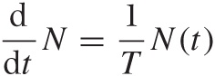
This equation is true for growth processes; for pure death processes instead we have an additional minus sign on the righthand side.
These equations can be solved or integrated explicitly, and their solutions are:
N(t) = N0 et/T | Pure birth process |
N(t) = N0 e–t/T | Pure death process |
Instead of using the “fraction” f of new or dying cells that we used in the difference equation, here we employ a characteristic time scale T, which is the time over which the number of cells changes by a factor e or 1/e, where e = 2.71828 .... The value for this time scale will depend on the actual system: for cells that multiply rapidly, T will be smaller than for another species that grows more slowly. Notice that such a scale factor must be there to make the argument of the exponential function dimensionally consistent! Furthermore, the parameter N0 is the number of cells in existence at the beginning t = 0.
Exponential processes (either birth or death) are very important, but they never last very long. In a pure death process, the population very quickly dwindles to practically nothing. At t = 3T, only 5 percent of the original population are left; at t = 10T, less than 1 in 10,000 of the original cells has survived; at t = 20T, we are down to one in a billion. In other words, after a time that is a small multiple of T, the population will have all but disappeared.
Pure birth processes face the opposite problem: the population grows so quickly that, after a very short while, it will exceed the capacity of its environment. This is so generally true that it is worth emphasizing: exponential growth is not sustainable over extended time periods. A process may start out as exponential, but before long, it must and will saturate. That brings us to the next scenario.
Constrained Growth: The Logistic Equation
Pure birth processes never continue for very long: the population quickly grows to a size that is unsustainable, and then the growth slows. A common model that takes this behavior into account assumes that the members of the population start to “crowd” each other, possibly competing for some shared resource such as food or territory. Mathematically, this can be expressed as follows:
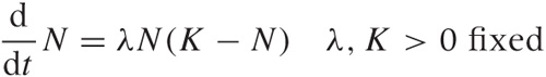
The first term on the righthand side (which equals λKN) is the same as in the exponential growth equation. By itself, it would lead to an exponentially growing population N(t) = C exp(λKt). But the second term (–λN2) counteracts this: it is negative, so its effect is to reduce the population; and it is proportional to N2, so it grows more strongly as N becomes large. (You can motivate the form of this term by observing that it measures the number of collisions between members of the population and therefore expresses the “crowding” effect.)
This equation is known as the logistic differential equation, and its solution is the logistic function:
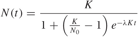
This is a complicated function that depends on three parameters:
λ | The characteristic growth rate |
K | The carrying capacity K = N(t → ∞) |
N0 | The initial number N0 = N(t = 0) of cells |
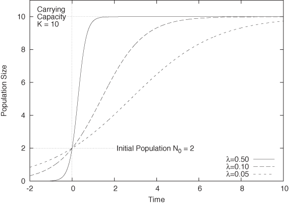
Compared to a pure (exponential) growth process, the appearance of the parameter K is new. It stands for the system’s “carrying capacity”—that is the maximum number of cells that the environment can support. You should convince yourself that the logistic function indeed tends to K as t becomes large. (You will find different forms of this function elsewhere and with different parameters, but the form given here is the most useful one.) Figure 8-6 shows the logistic function for a selection of parameter values.
I should point out that determining values for the three parameters from data can be extraordinarily difficult especially when the only data points available are those to the left of the inflection point (the point with maximum slope, about halfway between N0 and K). Many different combinations of λ, K, and N0 may seem to fit the data about equally well. In particular, it is difficult to assess K from early-stage data alone. You may want to try to obtain an independent estimate (even a very rough one) for the carrying capacity and use it when determining the remaining parameters from the data.
The logistic function is the most common model for all growth processes that exhibit some form of saturation. For example, infection rates for contagious diseases can be modeled using the logistic equation, as can the approach to equilibrium for cache hit rates.
Oscillations
The last of the common dynamical behaviors occurs in systems in which some quantity has an equilibrium value and that respond to excursions from that equilibrium position with a restoring effect, which drives the system back to the equilibrium position. If the system does not come to rest in the equilibrium position but instead overshoots, then the process will continue, going back and forth across the neutral position—in other words, the system undergoes oscillation. Oscillations occur in many physical systems (from tides to grandfather clocks to molecular bonds), but the “restore and overshoot” phenomenon is much more general. In fact, oscillations can be found almost everywhere: the pendulum that has “swung the other way” is proverbial, from the political scene to personal relationships.
Oscillations are periodic: the system undergoes the same motion again and again. The simplest functions that exhibit this kind of behavior are the trigonometric functions sin(x) and cos(x) (also see Appendix B), therefore we can express any periodic behavior, at least approximately, in terms of sines or cosines. Sine and cosine are periodic with period 2π. To express an oscillation with period D, we therefore need to rescale x by 2π/D. It may also be necessary to shift x by a phase factor ϕ: an expression like sin(2π(x – ϕ)/D) will at least approximately describe any periodic data set.
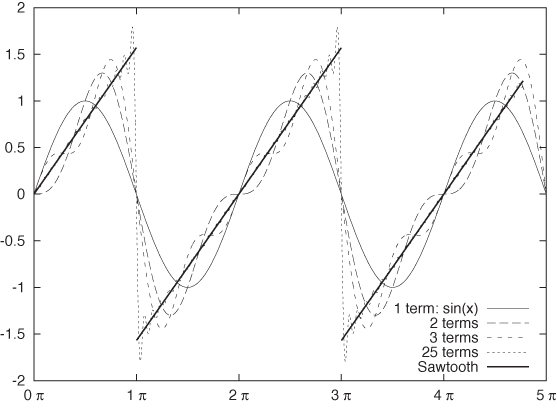
But it gets better: a powerful theorem states that every periodic function, no matter how crazy, can be written as a (possibly infinite) combination of trigonometric functions called a Fourier series. A Fourier series looks like this:
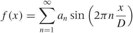
where I have assumed that ϕ = 0. The important point is that only integer multiples of 2π/D are being used in the argument of the sine—the so-called “higher harmonics” of sin(2π x/D). We need to adjust the coefficients an to describe a data set. Although the series is in principle infinite, we can usually get reasonably good results by truncating it after only a few terms. (We saw an example for this in Chapter 6, where we used the first two terms to describe the variation in CO2 concentration over Mauna Loa on Hawaii.)
If the function is known exactly, then the coefficients an can be worked out. For the sawtooth function (see Figure 8-7), the coefficients are simply 1, 1/2, 1/3, 1/4,... with alternating signs:
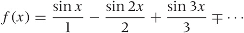
You can see that the series converges quite rapidly—even for such a crazy, discontinuous function as the sawtooth.
Case Study: How Many Servers Are Best?
To close out this chapter, let’s discuss an additional simple case study in model building.
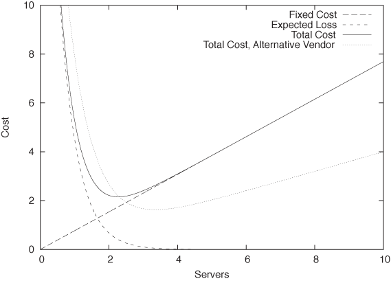
Imagine you are deciding how many servers to purchase to power your ecommerce site. Each server costs you a fixed amount E per day—this includes both the operational cost for power and colocation as well as the amortized acquisition cost (i.e., the purchase price divided by the number of days until the server is obsolete and will be replaced). The total cost for n servers is therefore nE.
Given the expected traffic, one server should be sufficient to handle the load. However, each server has a finite probability p of failing on any given day. If your site goes down, you expect to lose B in profit before a new server can be provisioned and brought back online. Therefore, the expected loss when using a single server is pB.
Of course, you can improve the reliability of your site by using multiple servers. If you have n servers, then your site will be down only if all of them fail simultaneously. The probability for this event is pn. (Note that pn < p, since p is a probability and therefore p < 1.)
The total daily cost C that you incur can now be written as the combination of the fixed cost nE and the expected loss due to server downtime pn B (also see Figure 8-8):
C = pn B + nE
Given p, B, and E, you would like to minimize this cost with respect to the number of servers n. We can do this either analytically (by taking the derivative of C with respect to n) or numerically.
But wait, there’s more! Suppose we also have an alternative proposal to provision our data center with servers from a different vendor. We know that their reliability q is worse (so that q > p), but their price F is significantly lower (F ≪ E). How does this variant compare to the previous one?
The answer depends on the values for p, B, and E. To make a decision, we must evaluate not only the location of the minimum in the total cost (i.e., the number of servers required) but also the actual value of the total cost at the minimum position. Figure 8-8 includes the total cost for the alternative proposal that uses less reliable but much cheaper servers. Although we need more servers under this proposal, the total cost is nevertheless lower than in the first one.
(We can go even further: how about a mix of different servers? This scenario, too, we can model in a similar fashion and evaluate it against its alternatives.)
Why Modeling?
Why worry about modeling in a book on data analysis? It seems we rarely have touched any actual data in the examples of this chapter.
It all depends on your goals when working with data. If all you want to do is to describe it, extract some features, or even decompose it fully into its constituent parts, then the “analytic” methods of graphical and data analysis will suffice. However, if you intend to use the data to develop an understanding of the system that produced the data, then looking at the data itself will be only the first (although important) step.
I consider conceptual modeling to be extremely important, because it is here that we go from the descriptive to the prescriptive. A conceptual model by itself may well be the most valuable outcome of an analysis. But even if not, it will at the very least enhance the purely analytical part of our work, because a conceptual model will lead us to additional hypothesis and thereby suggest additional ways to look at and study the data in an iterative process—in other words, even a purely conceptual model will point us back to the data but with added insight.
The methods described in this chapter and the next are the techniques that I have found to be the most practically useful when thinking about data and the processes that generated it. Whenever looking at data, I always try to understand the system behind it, and I always use some (if not all) of the methods from these two chapters.
Workshop: Sage
Most of the tools introduced in this book work with numbers, which makes sense given that we are mostly interested in understanding data. However, there is a different kind of tool that works with formulas instead: computer algebra systems. The big (commercial) brand names for such systems have been Maple and Mathematica; in the open source world, the Sage project (http://www.sagemath.org) has become somewhat of a front runner.
Sage is an “umbrella” project that attempts to combine several existing open source projects (SymPy, Maxima, and others) together with some added functionality into a single, coherent, Python-like environment. Sage places heavy emphasis on features for number theory and abstract algebra (not exactly everyone’s cup of tea) and also includes support for numerical calculations and graphics, but in this section we will limit ourselves to basic calculus and a little linear algebra. (A word of warning: if you are not really comfortable with calculus, then you probably want to skip the rest of this section. Don’t worry—it won’t be needed in the rest of the book.)
Once you start Sage, it drops you into a text-based command interpreter (a REPL, or read-eval-print loop). Sage makes it easy to perform some simple calculations. For example, let’s define a function and take its derivative:
sage: a, x = var( 'a x' )
sage: f(x) = cos(a*x)
sage: diff( f, x )
x |--> -a*sin(a*x)
In the first line we declare a and x
as symbolic variables—so that we can refer to them later and Sage
knows how to handle them. We then define a function using the
“mathematical” notation f(x) = ....
Only functions defined in this way can be used in symbolic
calculations. (It is also possible to define Python functions using
regular Python syntax, as in def f(x, a):
return cos(a*x), but such functions can only be evaluated
numerically.) Finally, we calculate the first derivative of the
function just defined.
All the standard calculus operations are available. We can combine functions to obtain more complex ones, we can find integrals (both definite and indefinite), and we can even evaluate limits:
sage: # Indefinite integral:
sage: integrate( f(x,a) + a*x^2, x )
1/3*a*x^3 + sin(a*x)/a
sage:
sage: # Definite integral on [0,1]:
sage: integrate( f(x,a) + a*x^2, x, 0, 1 )
1/3*(a^2 + 3*sin(a))/a
sage:
sage: # Definite integral on [0,pi], assigned to function:
sage: g(x,a) = integrate( f(x,a) + a*x^2, x, 0, pi )
sage:
sage: # Evaluate g(x,a) for different a:
sage: g(x,1)
1/3*pi^3
sage: g(x,1/2)
1/6*pi^3 + 2
sage: g(x,0)
----------------------------------------------------------
RuntimeError

(some output omitted...)
RuntimeError: power::eval(): division by zero
sage: limit( g(x,a), a=0 )
pi
In the next-to-last command, we tried to evaluate an expression
that is mathematically not well defined: the function g(x,a) includes a term of the form
sin(πa)/a, which we can’t
evaluate for a = 0 because we can’t divide by
zero. However, the limit 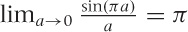 exists and is found by the
 limit() function.
As a final example from calculus, let’s evaluate some Taylor series (the arguments are: the function to expand, the variable to expand in, the point around which to expand, and the degree of the desired expansion):
sage: taylor( f(x,a), x, 0, 5 )
1/24*a^4*x^4 - 1/2*a^2*x^2 + 1
sage: taylor( sqrt(1+x), x, 0, 3 )
1/16*x^3 - 1/8*x^2 + 1/2*x + 1
So much for basic calculus. Let’s also visit an example from linear algebra. Suppose we have the linear system of equations:
ax + by | = 1 | |
2x + ay | + 3z | = 2 |
b2x | – z | = a |
and that we would like to find those values of (x, y, z) that solve this system. If all the coefficients were numbers, then we could use a numeric routine to obtain the solution; but in this case, some coefficients are known only symbolically (as a and b), and we would like to express the solution in terms of these variables.
Sage can do this for us quite easily:
sage: a, b, x, y, z = var( 'a b x y z' )
sage:
sage: eq1 = a*x + b*y == 1
sage: eq2 = 2*x + a*y + 3*z == 2
sage: eq3 = b^2 - z == a
sage:

sage: solve( [eq1,eq2,eq3], x,y,z )
[[x == (3*b^3 - (3*a + 2)*b + a)/(a^2 - 2*b),
  y == -(3*a*b^2 - 3*a^2 - 2*a + 2)/(a^2 - 2*b),
  z == b^2 - a]]
As a last example, let’s demonstrate how to calculate the eigenvalues of the following matrix:
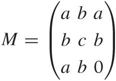
Again, if the matrix were given numerically, then we could use a numeric algorithm, but here we would like to obtain a symbolic solution.
Again, Sage can do this easily:
sage: m = matrix( [[a,b,a],[b,c,b],[a,b,0]] )
sage: m.eigenvalues()
[-1/18*(-I*sqrt(3) + 1)*(4*a^2 - a*c + 6*b^2 + c^2)/(11/54*a^3 - 7/18*a^2*c + 1/3
*b^2*c + 1/27*c^3 + 1/18*(15*b^2 - c^2)*a + 1/18*sqrt(-5*a^6 - 6*a^4*b^2 + 11*a^2
*b^4 - 5*a^2*c^4 - 32*b^6 + 2*(5*a^3 + 4*a*b^2)*c^3 + (5*a^4 - 62*a^2*b^2 - 4*b^4
)*c^2 - 2*(5*a^5 + 17*a^3*b^2 - 38*a*b^4)*c)*sqrt(3))^(1/3) - 1/2*(I*sqrt(3) + 1)
*(11/54*a^3 - 7/18*a^2*c + 1/3*b^2*c + 1/27*c^3 + 1/18*(15*b^2 - c^2)*a + 1/18*sq
rt(-5*a^6 - 6*a^4*b^2 + 11*a^2*b^4 - 5*a^2*c^4 - 32*b^6 + 2*(5*a^3 + 4*a*b^2)*c^3
 + (5*a^4 - 62*a^2*b^2 - 4*b^4)*c^2 - 2*(5*a^5 + 17*a^3*b^2 - 38*a*b^4)*c)*sqrt(3
))^(1/3) + 1/3*a + 1/3*c, -1/18*(I*sqrt(3) + 1)*(4*a^2 - a*c + 6*b^2 + c^2)/(11/5
4*a^3 - 7/18*a^2*c + 1/3*b^2*c + 1/27*c^3 + 1/18*(15*b^2 - c^2)*a + 1/18*sqrt(-5*
a^6 - 6*a^4*b^2 + 11*a^2*b^4 - 5*a^2*c^4 - 32*b^6 + 2*(5*a^3 + 4*a*b^2)*c^3 + (5*
a^4 - 62*a^2*b^2 - 4*b^4)*c^2 - 2*(5*a^5 + 17*a^3*b^2 - 38*a*b^4)*c)*sqrt(3))^(1/
3) - 1/2*(-I*sqrt(3) + 1)*(11/54*a^3 - 7/18*a^2*c + 1/3*b^2*c + 1/27*c^3 + 1/18*(
15*b^2 - c^2)*a + 1/18*sqrt(-5*a^6 - 6*a^4*b^2 + 11*a^2*b^4 - 5*a^2*c^4 - 32*b^6
+ 2*(5*a^3 + 4*a*b^2)*c^3 + (5*a^4 - 62*a^2*b^2 - 4*b^4)*c^2 - 2*(5*a^5 + 17*a^3*
b^2 - 38*a*b^4)*c)*sqrt(3))^(1/3) + 1/3*a + 1/3*c, 1/3*a + 1/3*c + 1/9*(4*a^2 - a
*c + 6*b^2 + c^2)/(11/54*a^3 - 7/18*a^2*c + 1/3*b^2*c + 1/27*c^3 + 1/18*(15*b^2 -
 c^2)*a + 1/18*sqrt(-5*a^6 - 6*a^4*b^2 + 11*a^2*b^4 - 5*a^2*c^4 - 32*b^6 + 2*(5*a
^3 + 4*a*b^2)*c^3 + (5*a^4 - 62*a^2*b^2 - 4*b^4)*c^2 - 2*(5*a^5 + 17*a^3*b^2 - 38
*a*b^4)*c)*sqrt(3))^(1/3) + (11/54*a^3 - 7/18*a^2*c + 1/3*b^2*c + 1/27*c^3 + 1/18
*(15*b^2 - c^2)*a + 1/18*sqrt(-5*a^6 - 6*a^4*b^2 + 11*a^2*b^4 - 5*a^2*c^4 - 32*b^
6 + 2*(5*a^3 + 4*a*b^2)*c^3 + (5*a^4 - 62*a^2*b^2 - 4*b^4)*c^2 - 2*(5*a^5 + 17*a^
3*b^2 - 38*a*b^4)*c)*sqrt(3))^(1/3)]
Whether these results are useful to us is a different question!
This last example demonstrates something I have found to be quite generally true when working with computer algebra systems: it can be difficult to find the right kind of problem for them. Initially, computer algebra systems seem like pure magic, so effortlessly do they perform tasks that took us years to learn (and that we still get wrong). But as we move from trivial to more realistic problems, it is often difficult to obtain results that are actually useful. All too often we end up with a result like the one in the eigenvalue example, which—although “correct”—simply does not shed much light on the problem we tried to solve! And before we try manually to simplify an expression like the one for the eigenvalues, we might be better off solving the entire problem with paper and pencil, because using paper and pencil, we can can introduce new variables for frequently occurring terms or even make useful approximations as we go along.
I think computer algebra systems are most useful in scenarios that require the generation of a very large number of terms (e.g., combinatorial problems), which in the end are evaluated (numerically or otherwise) entirely by the computer to yield the final result without providing a “symbolic” solution in the classical sense at all. When these conditions are fulfilled, computer algebra systems enable you to tackle problems that would simply not be feasible with paper and pencil. At the same time, you can maintain a greater level of accuracy because numerical (finite-precision) methods, although still required to obtain a useful result, are employed only in the final stages of the calculation (rather than from the outset). Neither of these conditions is fulfilled for relatively straightforward ad hoc symbolic manipulations. Despite their immediate “magic” appeal, computer algebra systems are most useful as specialized tools for specialized tasks!
One final word about the Sage project. As an open source project, it leaves a strange impression. You first become aware of this when you attempt to download the binary distribution: it consists of a 500 MB bundle, which unpacks to 2 GB on your disk! When you investigate what is contained in this huge package, the answer turns out to be everything. Sage ships with all of its dependencies. It ships with its own copy of all libraries it requires. It ships with its own copy of R. It ships with its own copy of Python! In short, it ships with its own copy of everything.
This bundling is partially due to the well-known difficulties with making deeply numerical software portable, but is also an expression of the fact that Sage is an umbrella project that tries to combine a wide range of otherwise independent projects. Although I sincerely appreciate the straightforward pragmatism of this solution, it also feels heavy-handed and ultimately unsustainable. Personally, it makes me doubt the wisdom of the entire “all under one roof” approach that is the whole purpose of Sage: if this is what it takes, then we are probably on the wrong track. In other words, if it is not feasible to integrate different projects in a more organic way, then perhaps those projects should remain independent, with the user free to choose which to use.
Further Reading
There are two or three dozen books out there specifically on the topic of modeling, but I have been disappointed by most of them. Some of the more useful (from the elementary to the quite advanced) include the following.
How to Model It: Problem Solving for the Computer Age. A. M. Starfield, K. A. Smith, and A. L. Bleloch. Interaction Book Company. 1994.
Probably the best elementary introduction to modeling that I am aware of. Ten (ficticious) case studies are presented and discussed, each demonstrating a different modeling method. (Available directly from the publisher.)
An Introduction to Mathematical Modeling. Edward A. Bender. Dover Publications. 2000. Short and idiosyncratic. A bit dated but still insightful.
Concepts of Mathematical Modeling. Walter J. Meyer. Dover Publications. 2004.
This book is a general introduction to many of the topics required for mathematical modeling at an advanced beginner level. It feels more dated than it is, and the presentation is a bit pedestrian; nevertheless, it contains a lot of accessible, and most of all practical, material.
Introduction to the Foundations of Applied Mathematics. Mark H. Holmes. Springer. 2009.
This is one of the few books on modeling that places recurring mathematical techniques, rather than case studies, at the center of its discussion. Much of the material is advanced, but the first few chapters contain a careful discussion of dimensional analysis and nice introductions to perturbation expansions and time-evolution scenarios.
Modeling Complex Systems. Nino Boccara. 2nd ed., Springer. 2010.
This is a book by a physicist (not a mathematician, applied or otherwise), and it demonstrates how a physicist thinks about building models. The examples are rich, but mostly of theoretical interest. Conceptually advanced, mathematically not too difficult.
Practical Applied Mathematics. Sam Howison. Cambridge University Press. 2005.
This is a very advanced book on applied mathematics with a heavy emphasis on partial differential equations. However, the introductory chapters, though short, provide one of the most insightful (and witty) discussions of models, modeling, scaling arguments, and related topics that I have seen.
The following two books are not about the process of modeling. Instead, they provide examples of modeling in action (with a particular emphasis on scaling arguments):
The Simple Science of Flight. Henk Tennekes. 2nd ed., MIT Press. 2009.
This is a short yet fascinating book about the physics and engineering of flying, written at the “popular science” level. The author makes heavy use of scaling laws throughout. If you are interested in aviation, then you will be interested in this book.
Scaling Concepts in Polymer Physics. Pierre-Gilles de Gennes. Cornell University Press. 1979.
This is a research monograph on polymer physics and probably not suitable for a general audience. But the treatment, which relies almost exclusively on a variety of scaling arguments, is almost elementary. Written by the master of the scaling models.
[15] A description of this data set can be found in A Handbook of Small Data Sets. David J. Hand, Fergus Daly, K. McConway, D. Lunn, and E. Ostrowski. Chapman & Hall/CRC. 1993.
[16] This story is reported in “Richard Feynman and the Connection Machine.” Daniel Hillis. Physics Today 42 (February 1989), p. 78. The paper can also be found on the Web.