Table of Contents for
Data Analysis with Open Source Tools
 Data Analysis with Open Source Tools
Published by
O'Reilly Media, Inc., 2010
Data Analysis with Open Source Tools
Published by
O'Reilly Media, Inc., 2010
- Cover
- Data Analysis with Open Source Tools
- O'Reilly Strata Conference
- Data Analysis with Open Source Tools
- Dedication
- A Note Regarding Supplemental Files
- Preface
- 1. Introduction
- I. Graphics: Looking at Data
- 2. A Single Variable: Shape and Distribution
- 3. Two Variables: Establishing Relationships
- 4. Time As a Variable: Time-Series Analysis
- 5. More Than Two Variables: Graphical Multivariate Analysis
- 6. Intermezzo: A Data Analysis Session
- II. Analytics: Modeling Data
- 7. Guesstimation and the Back of the Envelope
- 8. Models from Scaling Arguments
- 9. Arguments from Probability Models
- 10. What You Really Need to Know About Classical Statistics
- 11. Intermezzo: Mythbusting—Bigfoot, Least Squares, and All That
- III. Computation: Mining Data
- 12. Simulations
- 13. Finding Clusters
- 14. Seeing the Forest for the Trees: Finding Important Attributes
- 15. Intermezzo: When More Is Different
- IV. Applications: Using Data
- 16. Reporting, Business Intelligence, and Dashboards
- 17. Financial Calculations and Modeling
- 18. Predictive Analytics
- 19. Epilogue: Facts Are Not Reality
- A. Programming Environments for Scientific Computation and Data Analysis
- B. Results from Calculus
- C. Working with Data
- D. About the Author
- Index
- About the Author
- Colophon
- Copyright
Appendix B. Results from Calculus
IN THIS APPENDIX, WE REVIEW SOME OF THE RESULTS FROM CALCULUS THAT ARE EITHER NEEDED EXPLICITLY IN the main part of the book or are conceptually sufficiently important when doing data analysis and mathematical modeling that you should at least be aware that they exist.
Obviously, this appendix cannot replace a class (or two) in beginning and intermediate calculus, and this is also not the intent. Instead, this appendix should serve as a reminder of things that you probably know already. More importantly, the results are presented here in a slightly different context than usual. Calculus is generally taught with an eye toward the theoretical development—it has to be, because the intent is to teach the entire body of knowledge of calculus and therefore the theoretical development is most important. However, for applications you need a different sort of tricks (based on the same fundamental techniques, of course), and it generally takes years of experience to make out the tricks from the theory. This appendix assumes that you have seen the theory at least once, so I am just reminding you of it, but I want to emphasize those elementary techniques that are most useful in applications of the kind explained in this book.
This appendix is also intended as somewhat of a teaser: I have included some results that are particularly interesting, noteworthy, or fascinating as an invitation for further study.
The structure of this appendix is as follows:
To get a head start, we first look at some common functions and their graphs.
Then we discuss the core concepts of calculus proper: derivative, integral, limit.
Next I mention a few practical tricks and techniques that are frequently useful.
Near the end, there is a section on notation and very basic concepts. If you start feeling truly confused, check here! (I did not want to start with that section because I’m assuming that most readers know this material already.)
I conclude with some pointers for further study.
A note for the mathematically fussy: this appendix quite intentionally eschews much mathematical sophistication. I know that many of the statements can be made either more general or more precise. But the way they are worded here is sufficient for my purpose, and I want to avoid the obscurity that is the by-product of presenting mathematical statements in their most general form.
Common Functions
Functions are mappings, which map a real number into another real
number:  . This mapping is always unique: every input value
x is mapped to exactly one result value
f(x). (The converse is not
true: many input values may be mapped to the same result. For example,
the mapping f(x) = 0, which
maps all values to zero, is a valid
function.)
. This mapping is always unique: every input value
x is mapped to exactly one result value
f(x). (The converse is not
true: many input values may be mapped to the same result. For example,
the mapping f(x) = 0, which
maps all values to zero, is a valid
function.)
More complicated functions are often built up as combinations of simpler functions. The most important simple functions are powers, polynomials and rational functions, and trigonometric and exponential functions.
Powers
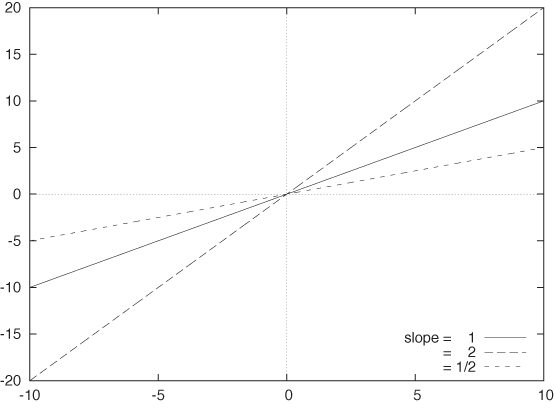
The simplest nontrivial function is the linear function:
f(x) = ax
The constant factor a is the slope: if x increases by 1, then f(x) increases by a. Figure B-1 shows linear functions with different slopes.
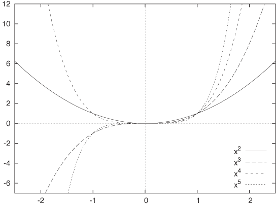
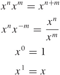
The next set of elementary functions are the simple powers:
f(x) = xk
The power k can be greater or smaller than 1. The exponent can be positive or negative, and it can be an integer or a fraction. Figure B-2 shows graphs of some functions with positive integer powers, and Figure B-3 shows functions with fractional powers.
Simple powers have some important properties:
Powers obey the following laws:
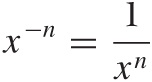
If the exponent is negative, it turns the expression into a fraction:
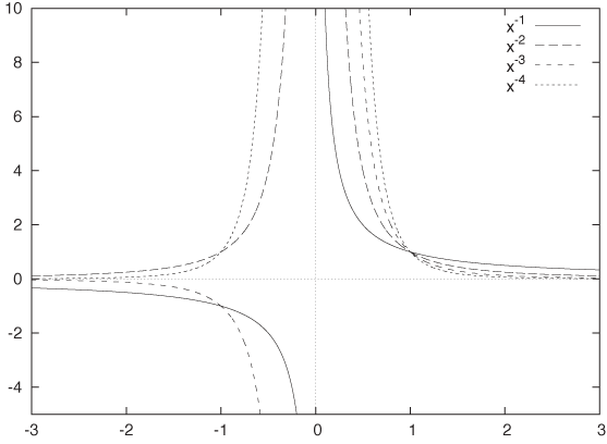
When dealing with fractions, we must always remember that the denominator must not become zero. As the denominator of a fraction approaches zero, the value of the overall expression goes to infinity. We say: the expression diverges and the function has a singularity at the position where the denominator vanishes. Figure B-4 shows graphs of functions with negative powers. Note the divergence for x = 0.
Polynomials and Rational Functions
Polynomials are sums of integer powers together with constant coefficients:
p(x) = anxn + an–1 xn–1 + ... + a2x2 + a1x + a0
Polynomials are nice because they are extremely easy to handle mathematically (after all, they are just sums of simple integer powers). Yet, more complicated functions can be approximated very well using polynomials. Polynomials therefore play an important role as approximations of more complicated functions.
All polynomials exhibit some “wiggles” and eventually diverge as x goes to plus or minus infinity (see Figure B-5). The highest power occurring in a polynomial is known as that degree of the polynomial.
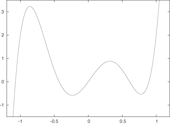
Rational functions are fractions that have polynomials in both the numerator and the denominator:
Although they may appear equally harmless, rational functions are entirely more complicated beasts than polynomials. Whenever the denominator becomes zero, they blow up. The behavior as x approaches infinity depends on the relative size of the largest powers in numerator and denominator, respectively. Rational functions are not simple functions.
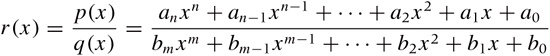
Exponential Function and Logarithm
Some functions cannot be expressed as polynomials (or as fraction of polynomials) of finite degree. Such functions are known as transcendental functions. For our purposes, the most important ones are the exponential function f(x) = ex (where e = 2.718281 ... is Euler’s number) and its inverse, the logarithm.
A graph of the exponential function is shown in Figure B-6. For positive argument the exponential function grows very quickly, and for negative argument it decays equally quickly. The exponential function plays a central role in growth and decay processes.
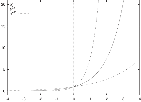
Some properties of the exponential function follow from the rules for powers:
The logarithm is the inverse of the exponential function; in other words:
y = ex | ⇔ | log y = x |
elog(x) = x | and | log (ex) = x |
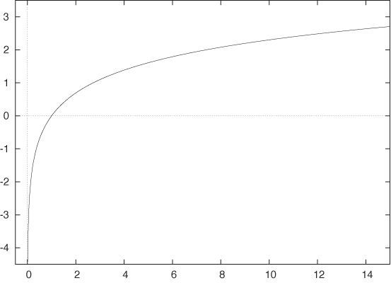
A plot of the logarithm is shown in Figure B-7. The logarithm is defined only for strictly positive values of x, and it tends to negative infinity as x approaches zero. In the opposite direction, as x becomes large the logarithm grows without bounds, but it grows almost unbelievably slowly. For x = 2, we have log 2 = 0.69 ... and for x = 10 we find log 10 = 2.30 ..., but for x = 1,000 and x = 106 we have only log 1000 = 6.91 ... and log 106 = 13.81 ..., respectively. Yet the logarithm does not have an upper bound: it keeps on growing but at an ever-decreasing rate of growth.
The logarithm has a number of basic properties:
log(1) = 0
log(x y) = log x + log y
log(xk) = k log x
As you can see, logarithms turn products into sums and powers into products. In other words, logarithms “simplify” expressions. This property was (and is!) used in numerical calculations: instead of multiplying two numbers (which is complicated), you add their logarithms (which is easy—provided you have a logarithm table or a slide rule) and then exponentiate the result. This calculational scheme is still relevant today, but not for the kinds of simple products that previous generations performed using slide rules. Instead, logarithmic multiplication can be necessary when dealing with products that would generate intermediate over- or underflows even though the final result may be of reasonable size. In particular, certain kinds of combinatorial and probabilistic problems require finding the maximum of expressions such as pn(1 – p)k, where p < 1 is a probability and n and k may be large numbers. Brute-force evaluation will underflow even for modest values of the exponents, but taking logarithms first will result in a numerically harmless expression.
Trigonometric Functions
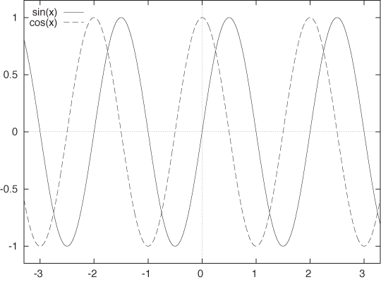
The trigonometric functions describe oscillations of all kinds and thus play a central role in sciences and engineering. Like the exponential function, they are transcendental functions, meaning they cannot be written down as a polynomial of finite degree.
Figure B-8 shows graphs of the two most important trigonometric functions: sin(x) and cos(x). The cosine is equal to the sine but is shifted by π/2 (90 degrees) to the left. We can see that both functions are periodic: they repeat themselves exactly after a period of length 2π. In other words, sin(x + 2π) = sin(x) and cos(x + 2π) = cos(x).
The length of the period is 2π, which you may recall is the circumference of a circle with radius equal to 1. This should make sense, because sin(x) and cos(x) repeat themselves after advancing by 2π and so does the circle: if you go around the circle once, you are back to where you started. This similarity between the trigonometric functions and the geometry of the circle is no accident, but this is not the place to explore it.
Besides their periodicity, the trigonometric functions obey a number of rules and properties (“trig identities”), only one of which is important enough to mention here:
sin2 x + cos2 x = 1 for all x
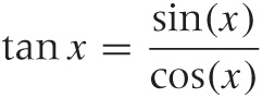
Finally, I should mention the tangent function, which is occasionally useful:
Gaussian Function and the Normal Distribution
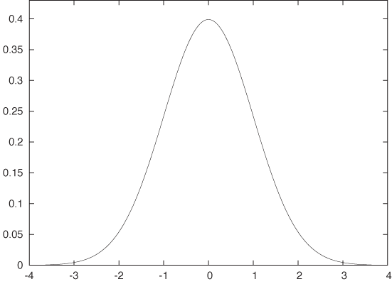
The Gaussian function arises frequently and in many different contexts. It is given by the formula:
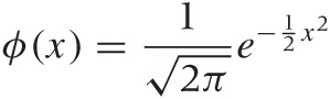
and its plot is shown in Figure B-9. (This
is the form in which the Gaussian should be memorized, with the factor
1/2 in the exponent and the factor  up front: they ensure that the integral of the
Gaussian over all x will be equal to 1.)
up front: they ensure that the integral of the
Gaussian over all x will be equal to 1.)
Two applications of the Gaussian stand out. First of all, a strong result from probability theory, the Central Limit Theorem states that (under rather weak assumptions) if we add many random quantities, then their sum will be distributed according to a Gaussian distribution. In particular, if we take several samples from a population and calculate the mean for each sample, then the sample means will be distributed according to a Gaussian. Because of this, the Gaussian arises all the time in probability theory and statistics.
It is because of this connection that the Gaussian is often identified as “the” bell curve—quite incorrectly so, since there are many bell-shaped curves, many of which have drastically different properties. In fact, there are important cases where the Central Limit Theorem fails, and the Gaussian is not a good way to describe the behavior of a random system (see the discussion of power-law distributions in Chapter 9).
The other context in which the Gaussian arises frequently is as a kernel—that is, as a strongly peaked and localized yet very smooth function. Although the Gaussian is greater than zero everywhere, it falls off to zero so quickly that almost the entire area underneath it is concentrated on the interval –3 ≤ x ≤ 3. It is this last property that makes the Gaussian so convenient to use as a kernel. Although the Gaussian is defined and nonzero everywhere (so that we don’t need to worry about limits of integration), it can be multiplied against almost any function and integrated. The integral will retain only those values of the function near zero; values at positions far from the origin will be suppressed (smoothly) by the Gaussian.
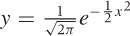
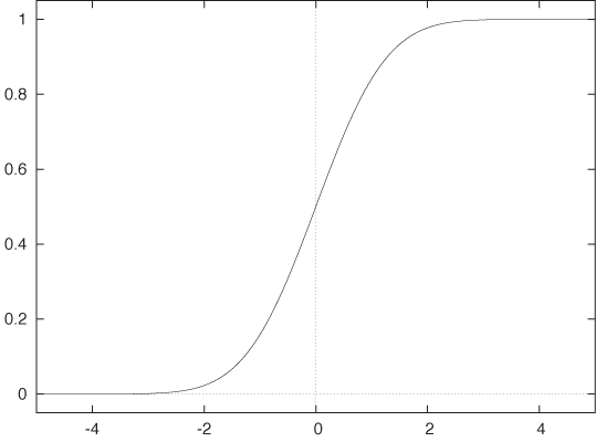
In statistical applications, we are often interested in the area under certain parts of the curve because that will provide the answer to questions such as: “What is the probability that the point lies between –1 and 1?” The antiderivative of the Gaussian cannot be expressed in terms of elementary functions; instead it is defined through the integral directly:
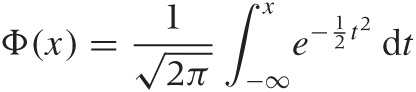
This function is known as the Normal distribution
function (see Figure B-10). As previously mentioned,
the factor  is a normalization constant that ensures the
area under the entire curve is 1.
is a normalization constant that ensures the
area under the entire curve is 1.
Given the function Φ(x), a question like the one just given can be answered easily: the area over the interval [–1, 1] is simply Φ(1) – Φ(–1).
Other Functions
There are some other functions that appear in applications often enough that we should be familiar with them but are a bit more exotic than the families of functions considered so far.
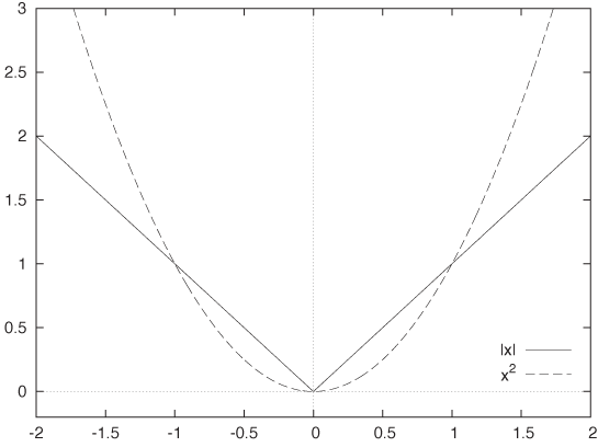
The absolute value function is defined as:
In other words, it is the positive (“absolute”) value of its argument. From a mathematical perspective, the absolute value is hard to work with because of the need to treat the two possible cases separately and because of the kink at x = 0, which poses difficulties when doing analytical work. For this reason, one instead often uses the square x2 to guarantee a positive value. The square relieves us of the need to worry about special cases explicitly, and it is smooth throughout. However, the square is relatively smaller than the absolute value for small values of x but relatively larger for large values of x. Weight functions based on the square (as in least-squares methods, for instance) therefore tend to overemphasize outliers (see Figure B-11).
Both the hyperbolic tangent tanh(x) (pronounced: tan-sh) and the logistic function are S-shaped or sigmoidal functions. The latter function is the solution to the logistic differential equation, hence the name. The logistic differential equation is used to model constrained growth processes such as bacteria competing for food and infection rates for contagious diseases. Both these functions are defined in terms of the exponential functions as follows:
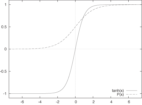
Both functions are smooth approximations to a step function, and they differ mostly in the range of values they assume: the tanh(x) takes on values in the interval [–1, 1], whereas the logistic function takes on only positive values between 0 and 1 (see Figure B-12). It is not hard to show that the two functions can be transformed into each other; in fact, we have P(x) = (tanh(x/2) + 1)/2.
These two functions are each occasionally referred to as the sigmoid function. That is incorrect: there are infinitely many functions that smoothly interpolate a step function. But among those functions, the two discussed here have the advantage that—although everywhere smooth—they basically consist of three straight lines: very flat as x goes to plus or minus infinity and almost linear in the transition regime. The position and steepness of the transition can be changed through a standard variable transformation; for example, tanh((x – m)/a) will have a transition at m with local slope 1/a.
The last function to consider here is the factorial: n!. The factorial is defined only for nonnegative integers, as follows:
0! = 1
n! = 1 · 2 ····· (n – 1) · n
The factorial plays an important role in combinatorial problems, since it is the number of ways that n distinguishable objects can be arranged. (To see this, imagine that you have to fill n boxes with n items. To fill the first box, you have n choices. To fill the second box, you have n – 1 choices. And so on. The total number of arrangements or permutations is therefore n · (n – 1) ··· 1 = n!.)
The factorial grows very quickly; it grows faster even than the exponential. Because the factorial grows so quickly, it is often convenient to work with its logarithm. An important and widely used approximation for the logarithm of the factorial is Stirling’s approximation:
log n! ≈ n log(n) – n | for large n |
For the curious: it is possible to define a function that smoothly interpolates the factorial for all positive numbers (not just integers). It is known as the Gamma function, and it is another example (besides the Gaussian distribution function) for a function defined through an integral:
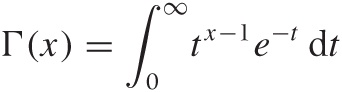
The variable t in this expression is just a “dummy” variable of integration—it does not appear in the final result. You can see that the first term in the integral grows as a power while the second falls exponentially, with the effect that the value of the integral is finite. Note that the limits of integration are fixed. The independent variable x enters the expression only as a parameter. Finally, it is easy to show that the Gamma function obeys the rule n Γ(n) = Γ(n + 1), which is the defining property of the factorial function.
We do not need the Gamma function in this book, but it is interesting as an example of how integrals can be used to define and construct new functions.
The Inverse of a Function
A function maps its argument to a result: given a value for x, we can find the corresponding value of f(x). Occasionally, we want to turn this relation around and ask: given a value of f(x), what is the corresponding value of x?
That’s what the inverse function does: if f(x) is some function, then its inverse f–1(x) is defined as the function that, when applied to f(x), returns the original argument:
f–1 (f(x)) = x
Sometimes we can invert a function explicitly. For example, if
f(x) =
x2, then the inverse
function is the square root, because  (which is the definition of the inverse
function). In a similar way, the logarithm is the inverse function of
the exponential:
log(ex) =
x.
(which is the definition of the inverse
function). In a similar way, the logarithm is the inverse function of
the exponential:
log(ex) =
x.
In other cases, it may not be possible to find an explicit form for the inverse function. For example, we sometimes need the inverse of the Gaussian distribution function Φ(x). However, no simple form for this function exists, so we write it symbolically as Φ–1(x), which refers to the function for which Φ–1 (Φ(x)) = x is true.
Calculus
Calculus proper deals with the consideration of limit processes: how does a sequence of values behave if we make infinitely many steps? The slope of a function and the area underneath a function are both defined through such limit processes (the derivative and the integral, respectively).
Calculus allows us to make statements about properties of functions and also to develop approximations.
Derivatives
We already mentioned the slope as the rate of change of a linear function. The same concept can be extended to nonlinear functions, though for such functions, the slope itself will vary from place to place. For this reason, we speak of the local slope of a curve at each point.
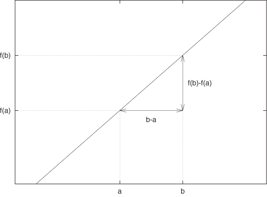
Let’s examine the slope as the rate of change of a function in more detail, because this concept is of fundamental importance whenever we want to interpolate or approximate some data by a smooth function. Figure B-13 shows the construction used to calculate the slope of a linear function. As x goes from a to b, the function changes from f(a) to f(b). The rate of change is the ratio of the change in f(x) to the change in x:
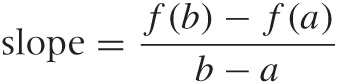
Make sure that you really understand this formula!
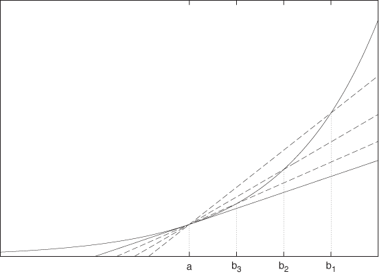
Now, let’s apply this concept to a function that is nonlinear. Because the slope of the curve varies from point to point, we cannot find the slope directly using the previous formula; however, we can use the formula to approximate the local slope.
Figure B-14
demonstrates the concept. We fix two points on a curve and put a
straight line through them. This line has a slope, which is
 . This is only an approximation to the slope at
point a. But we can improve the approximation by
moving the second point b closer to
a. If we let b go all the
way to a, we end up with the (local) slope
at the point a exactly. This
is called the derivative. (It is a central result
of calculus that, although numerator and denominator in
. This is only an approximation to the slope at
point a. But we can improve the approximation by
moving the second point b closer to
a. If we let b go all the
way to a, we end up with the (local) slope
at the point a exactly. This
is called the derivative. (It is a central result
of calculus that, although numerator and denominator in
 each go to zero separately in this process, the
fraction itself goes to a well-defined value.)
each go to zero separately in this process, the
fraction itself goes to a well-defined value.)
The construction just performed was done graphically and for a single point only, but it can be carried out analytically in a fully general way. The process is sufficiently instructive that we shall study a simple example in detail—namely finding a general rule for the derivative of the function f(x) = x2. It will be useful to rewrite the interval [a, b] as

[x, x + ϵ]. We can now go ahead and form the familiar ratio:
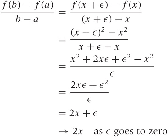
In the second step, the terms not depending on ϵ cancel each other; in the third step, we cancel an ϵ between the numerator and the denominator, which leaves an expression that is perfectly harmless as ϵ goes to zero! The (harmless) result is the sought-for derivative of the function. Notice that the result is true for any x, so we have obtained an expression for the derivative of x2 that holds for all x: the derivative of x2 is 2x. Always. Similar rules can be set up for other functions (you may try your hand at finding the rule for x3 or even xk for general k). Table B-1 lists a few of the most important ones.
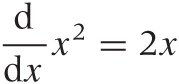
There are two ways to indicate the derivative. A short form uses
the prime, like this: f′(x)
is the derivative of f(x).
Another form uses the differential operator
 , which acts on the expression to its right.
Using the latter, we can write:
, which acts on the expression to its right.
Using the latter, we can write:
Finding Minima and Maxima
When a smooth function reaches a local minimum or maximum, its slope at that point is zero. This is easy to see: as you approach a peak, you go uphill (positive slope); once over the top, you go downhill (negative slope). Hence, you must have passed a point where you were going neither uphill nor downhill—in other words, where the slope was zero. (From a mathematically rigorous point of view, this is not quite as obvious as it may seem; you may want to check for “Rolle’s theorem” in a calculus text.)
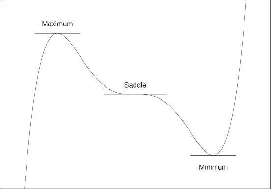
The opposite is also true: if the slope (i.e., the derivative) is zero somewhere, then the function has either a minimum or a maximum at that position. (There is also a third possibility: the function has a so-called saddle point there. In practice, this occurs less frequently.) Figure B-15 demonstrates all these cases.
We can therefore use derivatives to locate minima or maxima of a function. First we determine the derivative of the function, and then we find the locations where the derivative is zero (the derivative’s roots). The roots are the locations of the extrema of the original function.
Extrema are important because they are the solution to optimization problems. Whenever we want to find the “best” solution in some context, we are looking for an extremum: the lowest price, the longest duration, the greatest utilization, the highest efficiency. Hence, if we have a mathematical expression for the price, duration, utilization, or efficiency, we can take its derivative with respect to its parameters, set the derivative to zero, and solve for those values of the parameters that maximize (or minimize) our objective function.
Integrals
Derivatives find the local rate of change of a curve as the limit of a sequence of better and better approximations. Integrals calculate the area underneath a curve by a similar method.
Figure B-16 demonstrates the process. We approximate the area underneath a curve by using rectangular boxes. As we make the boxes narrower, the approximation becomes more accurate. In the limit of infinitely many boxes of infinitely narrow width, we obtain the exact area under the curve.
Integrals are conceptually very simple but analytically much more difficult than derivatives. It is always possible to find a closed-form expression for the derivative of a function. This is not so for integrals in general, but for some simple functions an expression for the integral can be found. Some examples are included in Table B-1.
Integrals are often denoted using uppercase letters, and there is a special symbol to indicate the “summing” of the area underneath a curve:
We can include the limits of the domain over which we want to integrate, like this:
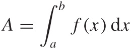
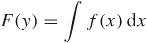
Notice that A is a number, namely the area underneath the curve between x = a and x = b, whereas the indefinite integral (without the limits) is a function, which can be evaluated at any point.
Limits, Sequences, and Series
The central concept in all of calculus is the notion of a limit. The basic idea is as follows. We construct some process that continues indefinitely and approximates some value ever more closely as the process goes on—but without reaching the limit in any finite number of steps, no matter how many. The important insight is that, even though the limit is never reached, we can nevertheless make statements about the limiting value. The derivative (as the limit of the difference ratio) and the integral (as the limit of the sum of approximating “boxes”) are examples that we have already encountered.
As simpler example, consider the numbers 1/1, 1/2, 1/3, 1/4, ... or 1/n in general as n goes to infinity. Clearly, the numbers approach zero ever more closely; nonetheless, for any finite n, the value of 1/n is always greater than zero. We call such an infinite, ordered set of numbers a sequence, and zero is the limit of this particular sequence.
A series is a sum:
As long as the number of terms in the series is finite, there is no problem. But once we let the number of terms go to infinity, we need to ask whether the sum still converges to a finite value. We have already seen a case where it does: we defined the integral as the value of the infinite sum of infinitely small boxes.
It may be surprising that an infinite sum can still add up to a finite value. Yet this can happen provided the terms in the sum become smaller rapidly enough. Here’s an example: if you sum up 1, 0.1, 0.01, 0.001, 0.0001, ..., you can see that the sum approaches 1.1111 ... but will never be larger than 1.2. Here is a more dramatic example: I have a piece of chocolate. I break it into two equal parts and give you one. Now I repeat the process with what I have left, and so on. Obviously, we can continue like this forever because I always retain half of what I had before. However, you will never accumulate more chocolate than what I started out with!
An infinite series converges to a finite value only if the magnitude of the terms decreases sufficiently quickly. If the terms do not become smaller fast enough, the series diverges (i.e., its value is infinite). An important series that does not converge is the harmonic series:
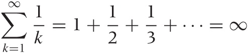
One can work out rigorous tests to determine whether or not a given series converges. For example, we can compare the terms of the series to those from a series that is known to converge: if the terms in the new series become smaller more quickly than in the converging series, then the new series will also converge.
Finding the value of an infinite sum is often tricky, but there is one example that is rather straightforward. The solution involves a trick well worth knowing. Consider the infinite geometric series:
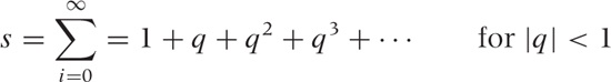
Now, let’s multiply by q and add 1:
qs + 1 | = q(1 + q + q2 + q3 + · · ·) + 1 |
= q + q2 + q3 + q4 + · · · + 1 | |
= s |
To understand the last step, realize that the righthand side equals our earlier definition of s. We can now solve the resulting equation for s and obtain:
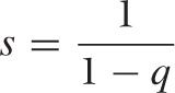
This is a good trick that can be applied in similar cases: if you can express an infinite series in terms of itself, the result may be an equation that you can solve explicitly for the unknown value of the infinite series.
Power Series and Taylor Expansion
An especially important kind of series contains consecutive powers of the variable x multiplied by the constant coefficients ai. Such series are called power series. The variable x can take on any value (it is a “dummy variable”), and the sum of the series is therefore a function of x:
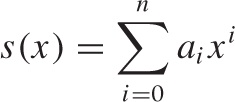
If n is finite, then there is only a finite number of terms in the series: in fact, the series is simply a polynomial (and, conversely, every polynomial is a finite power series). But the number of terms can also be infinite, in which case we have to ask for what values of x does the series converge. Infinite power series are of great theoretical interest because they are a (conceptually straightforward) generalization of polynomials and hence represent the “simplest” nonelementary functions.
But power series are also of the utmost practical importance. The reason is a remarkable result known as Taylor’s theorem. Taylor’s theorem states that any reasonably smooth function can be expanded into a power series. This process (and the resulting series) is known as the Taylor expansion of the function.
Taylor’s theorem gives an explicit construction for the coefficients in the series expansion:

In other words, the coefficient of the nth term is the nth derivative (evaluated at zero) divided by n!. The Taylor series converges for all x—the factorial in the denominator grows so quickly that convergence is guaranteed no matter how large x is.
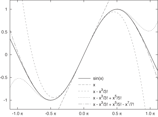
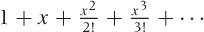
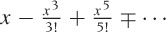
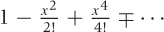
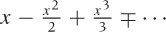
The Taylor series is an exact representation of the function on the lefthand side if we retain all (infinitely many) terms. But we can also truncate the series after just a few terms and so obtain a good local approximation of the function in question. The more terms we keep, the larger will be the range over which the approximation is good. For the sine function, Figure B-17 shows how the Taylor expansion improves as a greater number of terms is kept. Table B-2 shows the Taylor expansions for some functions we have encountered so far.
It is this last step that makes Taylor’s theorem so useful from a practical point of view: it tells us that we can approximate any smooth function locally by a polynomial. And polynomials are always easy to work with—often much easier than the complicated functions that we started with.
One important practical point: the approximation provided by a
truncated Taylor series is good only locally—that
is, near the point around which we expand. This is because in that
case x is small (i.e.,
x ≪ 1) and so higher powers become negligible
fast. Taylor series are usually represented in a form that assumes
that the expansion takes place around zero. If this is not the case,
we need to remove or factor out some large quantity so that we are
left with a “small parameter” in which to expand. As an example,
suppose we want to obtain an approximation to
ex for values of
x near 10. If we expanded in the usual fashion
around zero, then we would have to sum many terms
before the approximation becomes good (the terms grow until
10n < n!, which
means we need to keep more than 20 terms). Instead, we proceed as
follows: we write  . In other words, we set it up so that δ is
small allowing us to expand
eδ around zero as
before.
. In other words, we set it up so that δ is
small allowing us to expand
eδ around zero as
before.

Another important point to keep in mind is that the function must be smooth at the point around which we expand: it must not have a kink or other singularity there. This is why the logarithm is usually expanded around one (not zero): recall that the logarithm diverges as x goes to zero.
Useful Tricks
The Binomial Theorem
Probably everyone has encountered the binomial formulas at some point:
(a + b)2 = a2 + 2ab + b2
(a – b)2 = a2 – 2ab + b2
The binomial theorem provides an extension of this result to higher powers. The theorem states that, for an arbitrary integer power n, the expansion of the lefthand side can be written as:
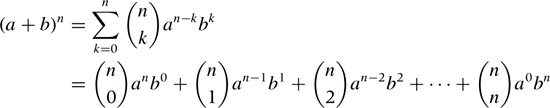
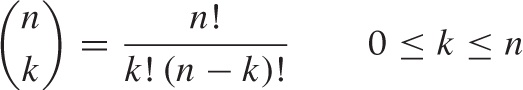
This complicated-looking expression involves the binomial coefficients:
The binomial coefficients are combinatorial factors that count the number of different ways one can choose k items from a set of n items, and in fact there is a close relationship between the binomial theorem and the binomial probability distribution.
As is the case for many exact results, the greatest practical use of the binomial theorem comes from an approximate expression. Assume that b < a, so that b/a < 1. Now we can write:
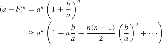
Here we have neglected terms involving higher powers of b/a, which are small compared to the retained terms, since b/a < 1 by construction (so that higher powers of b/a, which involve multiplying a small number repeatedly by itself, quickly become negligible).
In this form, the binomial theorem is frequently useful as a way to generate approximate expansions. In particular, the first-order approximation:
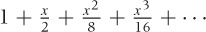
(1 + x)n ≈ 1 + nx | for |x| < 1 |
should be memorized.
The Linear Transformation
Here is a quick, almost trivial, trick that is useful enough to be committed to memory. Any variable can be transformed to a similar variable that takes on only values from the interval [0, 1], via the following linear transformation, where xmin and xmax are the minimum and maximum values that x can take on:
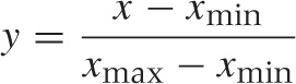
This transformation is frequently useful—for instance, if we have two quantities and would like to compare how they develop over time. If the two quantities have very different magnitudes, then we need to reduce both of them to a common range of values. The transformation just given does exactly that.
If we want the transformed quantity to fall whenever the original quantity goes up, we can do this by writing:
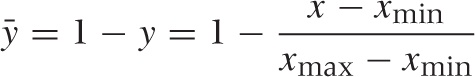
We don’t have to shift by xmin and rescale by the original range xmax – xmin. Instead, we can subtract any “typical” value and divide by any “typical” measure of the range. In statistical applications, for example, it is frequently useful to subtract the mean μ and to divide by the standard deviation σ. The resulting quantity is referred to as the z-score:
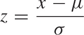
Alternatively, you might also subtract the median and divide by the inter-quartile range. The exact choice of parameters is not crucial and will depend on the specific application context. The important takeaway here is that we can normalize any variable by:
Subtracting a typical value (shifting) and
Dividing by the typical range (rescaling)
Dividing by Zero
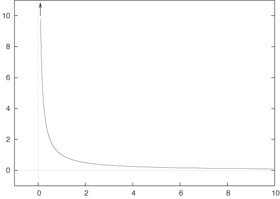
Please remember that you cannot divide by zero! I am sure you know this—but it’s surprisingly easy to forget (until the computer reminds us with a fatal “divide by zero” error).
It is instructive to understand what happens if you try to divide by zero. Take some fixed number (say, 1), and divide it by a sequence of numbers that approach zero:
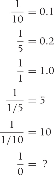
In other words, as you divide a constant by numbers that approach zero, the result becomes larger and larger. Finally, if you let the divisor go to zero, the result grows beyond all bounds: it diverges. Figure B-18 shows this graphically.
What you should take away from this exercise and Figure B-18 is that you cannot replace 1/0 by something else—for instance, it is not a smart move to replace 1/0 by 0 “because both don’t really mean anything, anyway.” If you need to find a numeric value for 1/0, then it should be something like “infinity,” but this is not a useful value to operate with in practical applications.
Therefore, whenever you encounter a fraction
 of any kind, you must
check whether the denominator can become zero and exclude
these points from consideration.
of any kind, you must
check whether the denominator can become zero and exclude
these points from consideration.
Failing to do so is one of the most common sources of error. What is worse, these errors are difficult to recover from—not just in implementations but also conceptually. A typical example involves “relative errors,” where we divide the difference between the observed and the expected value by the expected value:

What happens if for one day the expected value drops to zero? You are toast. There is no way to assign a meaningful value to the error in this case. (If the observed value is also zero, then you can treat this as a special case and define the relative error to be zero in this case, but if the observed value is not zero, then this definition is obviously inappropriate.)
These kinds of problems have an unpleasant ability to sneak up on you. A quantity such as the relative error or the defect rate (which is also a ratio: the number of defects found divided by the number of units produced) is a quantity commonly found in reports and dashboards. You don’t want your entire report to crash because no units were produced for some product on this day rendering the denominator zero in one of your formulas!
There are a couple of workarounds, neither of which is perfect.
In the case of the defect rate, where you can be sure that the
numerator will be zero if the denominator is (because no defects can
be found if no items were produced), you can add a small positive
number to the denominator and thereby prevent it from ever becoming
exactly zero. As long as this number is small compared to the number
of items typically produced in a day, it will not significantly affect
the reported defect rate, but will relieve you from having to check
for the  special case explicitly. In the case of
calculating a relative error, you might want to replace the numerator
with the average of the expected and the observed values. The
advantage is that now the denominator can be zero only if the
numerator is zero, which brings us back to the suggestion for dealing with
defect rates just discussed. The problem with this method is that when
no events are observed but some number was expected, the relative
error is reported as –2 (negative 200 percent instead of negative 100
percent); this is due to the factor 1/2 in the denominator, which
comes from calculating the average there.
special case explicitly. In the case of
calculating a relative error, you might want to replace the numerator
with the average of the expected and the observed values. The
advantage is that now the denominator can be zero only if the
numerator is zero, which brings us back to the suggestion for dealing with
defect rates just discussed. The problem with this method is that when
no events are observed but some number was expected, the relative
error is reported as –2 (negative 200 percent instead of negative 100
percent); this is due to the factor 1/2 in the denominator, which
comes from calculating the average there.
So, let me say it again: whenever you are dealing with fractions, you must consider the case of denominators becoming zero. Either rule them out or handle them explicitly.
Notation and Basic Math
This section is not intended as a comprehensive overview of mathematical notation or as your first introduction to mathematical formulas. Rather, it should serve as a general reminder of some basic facts and to clarify some conventions used in this book. (All my conventions are pretty standard—I have been careful not to use any symbols or conventions that are not generally used and understood.)
On Reading Formulas
A mathematical formula combines different components, called
terms, by use of operators. The most basic
operators are plus and minus
(+ and –) and multiplied by and divided
by (· and /). Plus and minus are always written explicitly,
but the multiplication operator is usually silent—in other words, if
you see two terms next to each other, with nothing between them, they
should be multiplied. The division operator can be written in two
forms: 1/n or  , which mean exactly the same thing. The former
is more convenient in text such as this; the latter is more clear for
long, “display” equations. An expression such as
1/n + 1 is ambiguous and should not be used, but
if you encounter it, you should assume that it means
, which mean exactly the same thing. The former
is more convenient in text such as this; the latter is more clear for
long, “display” equations. An expression such as
1/n + 1 is ambiguous and should not be used, but
if you encounter it, you should assume that it means
 and not 1/(n + 1) (which
is equivalent to
and not 1/(n + 1) (which
is equivalent to  ).
).
Multiplication and division have higher precedence than addition and subtraction, therefore ab + c means that first you multiply a and b and then add c to the result. To change the priority, you need to use parentheses: a(b + c) means that first you add b and c and then multiply the result by a. Parentheses can either be round (...) or square [...], but their meaning is the same.
Functions take one (or several) arguments and return a result. A function always has a name followed by the arguments. Usually the arguments are enclosed in parentheses: f(x). Strictly speaking, this notation is ambiguous because an expression such as f (a + b) could mean either “add a and b and then multiply by f” or “add a and b and then pass the result to the function f.” However, the meaning is usually clear from the context.
(There is a slightly more advanced way to look at this. You can
think of f as an operator, similar to a
differential operator like  or an integral operator like ∫
dt. This operator is now applied to the
expression to the right of it. If f is a
function, this means applying the function to the argument; if the operator is a
differential operator, this means taking the derivative; and if
f is merely a number, then applying it simply
means multiplying the term on its right by it.)
or an integral operator like ∫
dt. This operator is now applied to the
expression to the right of it. If f is a
function, this means applying the function to the argument; if the operator is a
differential operator, this means taking the derivative; and if
f is merely a number, then applying it simply
means multiplying the term on its right by it.)
A function may take more than one argument; for example, the function f (x, y, z) takes three arguments. Sometimes you may want to emphasize that not all of these arguments are equivalent: some are actual variables, whereas others are “parameters,” which are kept constant while the variables change. Consider f(x) = ax + b. In this function, x is the variable (the quantity usually plotted along the horizontal axis) while a and b would be considered parameters. If we want to express that the function f does depend on the parameters as well as on the actual variable, we can do this by including the parameters in the list of arguments: f (x, a, b). To visually separate the parameters from the actual variable (or variables), a semicolon is sometimes used: f (x; a, b). There are no hard-and-fast rules for when to use a semicolon instead of a comma—it’s simply a convenience that is sometimes used and other times not.
One more word on functions: several functions are regarded as “well known” in mathematics (such as sine and cosine, the exponential function, and the logarithm). The names of such well-known functions are always written in upright letters, whereas functions in general are denoted by an italic letter. (Variables are always written in italics.) For well-known functions, the parentheses around the arguments can be omitted if the argument is sufficiently simple. (This is another example of the “operator” point of view mentioned earlier.) Thus we may write sin(x + 1) + log x – f(x) (note the upright letters for sine and logarithm, and the parentheses around the argument for the logarithm have been omitted, because it consists of only a single term). This has a different meaning than: sin(x + 1) + log(x – f(x)).
Elementary Algebra
For numbers, the following is generally true:
a(b + c) = ab + ac
This is often applied in situations like the following, where we factor out the a:
a + b = a(1 + b/a)
If a is much greater than b, then we have now converted the original expression a + b into another expression of the form:
something large · (1 + something small)
which makes it easy to see which terms matter and which can be neglected in an approximation scheme. (The small term in the parentheses is “small” compared to the 1 in the parentheses and can therefore be treated as a perturbation.)
Quantities can be multiplied together, which gives rise to powers:
a · a = a2
a · a · a = a3
. . .
The raised quantity (the superscript) is also referred to as the exponent. In this book, superscripts always denote powers.
The three binomial formulas should be committed to memory:
(a + b)2 = a2 + 2ab + b2
(a – b)2 = a2 – 2ab + b2
(a + b)(a – b) = a2 – b2
Because the easiest things are often the most readily forgotten, let me just work out the first of these identities explicitly:
(a + b)2 | = (a + b)(a + b) |
= a(a + b) + b(a + b) | |
= a2 + ab + ba + b2 | |
= a2 + 2ab + b2 |
where I have made use of the fact that ab = ba.
Working with Fractions
Let’s review the basic rules for working with fractions. The expression on top is called the numerator, the one at the bottom is the denominator:
If you can factor out a common factor in both numerator and denominator, then this common factor can be canceled:
To add two fractions, you have to bring them onto a common denominator in an operation that is the opposite of canceling a common factor:
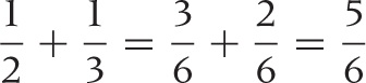
Here is a numeric example:
Sets, Sequences, and Series
A set is a grouping of elements in no particular order. In a sequence, the elements occur in a fixed order, one after the other.
The individual elements of sets and sequences are usually shown with subscripts that denote the index of the element in the set or its position in the sequence (similar to indexing into an array). In this book, subscripts are used only for the purpose of indexing elements of sets or sequences in this way.
Sets are usually indicated by curly braces. The following expressions are equivalent:
{x1, x2, x3, . . ., xn}
{xi | i = 1, . . ., n}
For brevity, it is customary to suppress the range of the index if it can be understood from context. For example, if it is clear that there are n elements in the set, I might simply write {xi}.
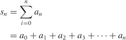
One often wants to sum a finite or infinite sequence of numbers; the result is known as a series:
x1 + x2 + x3 + · · · + xn
Instead of writing out the terms explicitly, it is often useful to use the sum notation:
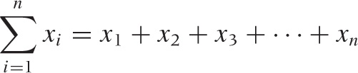
The meaning of the summation symbol should be clear from this
example. The variable used as index (here, i) is
written underneath the summation sign followed by the lower limit
(here, 1). The upper limit (here, n) is written
above the summation sign. As a shorthand, any one of these
specifications can be omitted. For instance, if it is clear from the
context that the lower limit is 1 and the upper limit is
n, then I might simply write  or even
  . In the latter form, it is understood that the
sum runs over the index of the summands.
. In the latter form, it is understood that the
sum runs over the index of the summands.
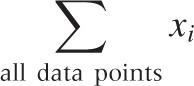
It is often convenient to describe the terms to be summed over in words, rather than giving specific limits:
Some standard transformations involving the summation notation are used fairly often. For example, one frequently needs to shift indices. The following three expressions are equal, as you can easily see by writing out explicitly the terms of the sum in each case:
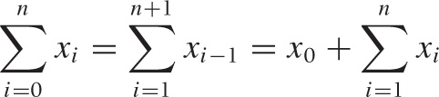
Keep in mind that the summation notation is just a shorthand for the explicit form given at the start of this section. If you become confused, you can always write out the terms explicitly to understand what is going on.
Finally, we may take the upper limit of the sum to be infinity, in which case the sum runs over infinitely many terms. Infinite series play a fundamental role in the theoretical development of mathematics, but all series that you will encounter in applications are, of course, finite.
Special Symbols
A few mathematical symbols are either indispensable or so useful that I wouldn’t do without them.
Binary relationships
There are several special symbols to describe the relationship between two expressions. Some of the most useful ones are listed in Table B-3.
Operator | Meaning |
= ≠ | equal to, not equal to |
< > | less than, greater than |
≤ ≥ | less than or equal to, greater than or equal to |
≪ ≫ | much less than, much greater than |
α | proportional to |
≈ | approximately equal to |
~ | scales as |
The last three might require a word of explanation. We say two quantities are approximately equal when they are equal up to a “small” error. Put differently, the difference between the two quantities must be small compared to the quantities themselves: x and 1.1x are approximately equal, x ≈ 1.1x, because the difference (which is 0.1x) is small compared to x.
One quantity is proportional to another if they are equal up to a constant factor that has been omitted from the expression. Often, this factor will have units associated with it. For example, when we say “time is money,” what we really mean is:
money α time
Here the omitted constant of proportionality is the hourly rate (which is also required to fix the units: hours on the left, dollars on the right; hence hourly rate must have units of “dollars per hour” to make the equation dimensionally consistent).
We say that a quantity scales as some other quantity if we want to express how one quantity depends on another one in a very general way. For example, recall that the area of a circle is πr2 (where r is the length of the radius) but that the area of a square is a2 (where a is the length of the side of the square). We can now say that “the area scales as the square of the length.” This is a more general statement than saying that the area is proportional to the square of the length: the latter implies that they are equal up to a constant factor, whereas the scaling behavior allows for more complicated dependencies. (In this example, the constant of proportionality depends on the shape of the figure, but the scaling behavior area ~ length2 is true for all symmetrical figures.)
In particular when evaluating the complexity of algorithms,
there is another notation to express a very similar notion: the
so-called big O notation. For example, the
expression  (n2)
states that the complexity of an algorithm grows (“scales”) with the
square of the number of elements in the input.
(n2)
states that the complexity of an algorithm grows (“scales”) with the
square of the number of elements in the input.
Parentheses and other delimiters
Round parentheses (...) are used for two purposes: to group terms together (establishing precedence) and to indicate the arguments to a function:
ab + c ≠ a(b + c) | Parentheses to establish precedence |
f(x, y) = x + y | Parentheses to indicate function arguments |
Square brackets [...] are mostly used to indicate an interval:
[a, b] | all x such that a ≤ x ≤ b |
For the purpose of this book, we don’t need to worry about the distinction between closed and open intervals (i.e., intervals that do or don’t contain their endpoints, respectively).
Very rarely I use brackets for other purposes—for example as an alternative to round parentheses to establish precedence, or indicate that a function takes another function as its argument, as in the expectation value: E[ f(x)].
Curly braces {...} always denote a set.
Miscellaneous symbols
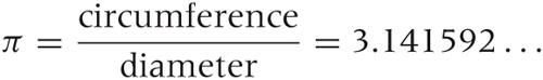
Two particular constants are indispensable. Everybody has heard of π = 3.141592 ..., which is the ratio of the circumference of a circle to its diameter:
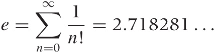
Equally important is the “base of the natural logarithm” e = 2.718281 ..., sometimes called Euler’s number. It is defined as the value of the infinite series:
The function ex obtained by raising e to the xth power has the property that its derivative also equals ex, and it is the only function that equals its derivative (up to a multiplicative constant, to be precise).
The number e also shows up in the definition of the Gaussian function:
e–x2
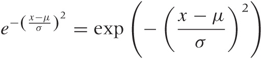
(Any function that contains e raised to –x2 power is called a “Gaussian”; what’s crucial is that the x in the exponent is squared and enters with a negative sign. Other constants may appear also, but the –x2 in the exponent is the defining property.)
Because the exponents are often complicated expressions themselves, there is an alternative notation for the exponential function that avoids superscripts and instead uses the function name exp(...). The expression exp(x) means exactly the same as ex, and the following two expressions are equivalent, also—but the one on the right is easier to write:
A value of infinite magnitude is indicated by a special symbol:
∞ | a value of infinite magnitude |
The square root sign  states that:

Finally, the integral sign ∫, which always occurs together with an expression of the form dx (or dt, or so), is used to denote a generalized form of summation: the expression to the right of the integral sign is to be “summed” for all values of x (or t). If explicit limits of the integration are given, they are attached to the integral sign:
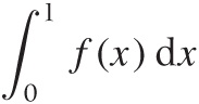
This means: “sum all values of f(x) for x ranging from 0 to 1.”
The Greek Alphabet
Greek letters are used all the time in mathematics and other sciences and should be committed to memory. (See Table B-4.)
Where to Go from Here
This appendix can of course only give a cartoon version of the topics mentioned, or—if you have seen this material before—at best serve as a reminder. But most of all, I hope it serves as a teaser: mathematics is a wonderfully rich and stimulating topic, and I would hope that in this appendix (and in the rest of this book) I have been able to convey some of its fascination—and perhaps even convinced you to dig a little deeper.
If you want to learn more, here are a couple of hints.
The first topic to explore is calculus (or real analysis). All modern mathematics starts here, and it is here that some of the most frequently used concepts (derivative, integral, Taylor expansion) are properly introduced. It is a must-have.
But if you limit your attention to calculus, you will never get over the idea that mathematics is about “calculating something.” To get a sense of what math is really all about, you have to go beyond analysis. The next topic in a typical college syllabus is linear algebra. In linear algebra, we go beyond relatively tangible things like curves and numbers and for the first time start to consider concepts in a fully abstract way: spaces, transformations, mappings. What can we say about them in general without having to appeal to any particular realization? Understanding this material requires real mental effort—you have to change the way you think. (Similarly to how you have to change the way you think if you try to learn Lisp or Haskell.) Linear algebra also provides the theoretical underpinnings of all matrix operations and hence for most frequently used numerical routines. (You can’t do paper-and-pencil mathematics without calculus, and you can’t do numerical mathematics without linear algebra.)
With these two subjects under your belt, you will be able to pick up pretty much any mathematical topic and make sense of it. You might then want to explore complex calculus for the elegance and beauty of its theorems, or functional analysis and Fourier theory (which blend analysis and linear algebra) because of their importance in all application-oriented areas, or take a deeper look at probability theory, with its obvious importance for anything having to do with random data.
On Math
I have observed that there are two misconceptions about mathematics that are particularly prevalent among people coming from a software or computing background. The first misconception holds that mathematics is primarily a prescriptive, calculational (not necessarily numerical) scheme and similar to an Algol-derived programming language: a pseudo-code for expressing algorithms. The other misconception views mathematics as mostly an abstract method for formal reasoning, not dissimilar to certain logic programming environments: a way to manipulate logic statements.
What both of them miss is that mathematics is not a method but first and foremost a body of content in its own right. You will never understand what mathematics is if you see it only as something you use to obtain certain results. Mathematics is, first and foremost, a rich and exciting story in itself.
There is an unfortunate perception among nonmathematicians (and even partially reinforced by this book) that mathematics is about “calculating things.” This is not so, and it is probably the most unhelpful misconception about mathematics of all.
In fairness, this point of view is promulgated by many introductory college textbooks. In a thoroughly misguided attempt to make their subject “interesting,” they try to motivate mathematical concepts with phony applications to the design of bridges and airplanes, or to calculating the probability of winning at poker. This not only obscures the beauty of the subject but also creates the incorrect impression of mathematics as a utilitarian fingering exercise and almost as a necessary evil.
Finally, I strongly recommend that you stay away from books on popular or recreational math, for two reasons. First, they tend to focus on a small set of topics that can be treated using “elementary” methods (mostly geometry and some basic number theory), and tend to omit most of the conceptually important topics. Furthermore, in their attempt to present amusing or entertaining snippets of information, they fail to display the rich, interconnected structure of mathematical theory: all you end up with is a book of (stale) jokes.
Further Reading
Calculus
The Hitchhiker’s Guide to Calculus. Michael Spivak. Mathematical Association of America. 1995.
If the material in this appendix is really new to you, then this short (120-page) booklet provides a surprisingly complete, approachable, yet mathematically respectable introduction. Highly recommended for the curious and the confused.
Precalculus: A Prelude to Calculus. Sheldon Axler. Wiley. 2008.
Axler’s book covers the basics: numbers, basic algebra, inequalities, coordinate systems, and functions—including exponential, logarithmic, and trigonometric functions—but it stops short of derivatives and integrals. If you want to brush up on foundational material, this is an excellent text.
Calculus. Michael Spivak. 4th ed., Publish or Perish. 2008.
This is a comprehensive book on calculus. It concentrates exclusively on the clear development of the mathematical theory and thereby avoids the confusion that often results from an oversupply of (more or less) artificial examples. The presentation is written for the reader who is relatively new to formal mathematical reasoning, and the author does a good job motivating the peculiar arguments required by formal mathematical manipulations. Rightly popular.
Yet Another Introduction to Analysis. Victor Bryant. Cambridge University Press. 1990.
This short book is intended as a quick introduction for those readers who already possess passing familiarity with the topic and are comfortable with abstract operations.
Linear Algebra
Linear Algebra Done Right. Sheldon Axler. 2nd ed., Springer. 2004.
This is the best introduction to linear algebra that I am aware of, and it fully lives up to its grandiose title. This book treats linear algebra as abstract theory of mappings, but on a very accessible, advanced undergraduate level. Highly recommended.
Linear Algebra. Klaus Jänich. Springer. 1994.
This book employs a greater amount of abstract mathematical formalism than the previous entry, but the author tries very hard to explain and motivate all concepts. This book might therefore give a better sense of the nature of abstract algebraic arguments than Axler’s streamlined presentation. The book is written for a first-year course at German universities; the style of the presentation may appear exotic to the American reader.
Complex Analysis
Complex Analysis. Joseph Bak and Donald J. Newman. 2nd ed., Springer. 1996.
This is a straightforward, and relatively short, introduction to all the standard topics of classical complex analysis.
Complex Variables. Mark J. Ablowitz and Athanassios S. Fokas. 2nd ed., Cambridge University Press. 2003.
This is a much more comprehensive and advanced book. It is split into two parts: the first part developing the theory, the second part discussing several nontrivial applications (mostly to the theory of differential equations).
Fourier Analysis and Its Applications. Gerald B. Folland. American Mathematical Society. 2009.
This is a terrific introduction to Fourier theory. The book places a strong emphasis on the solution of partial differential equations but in the course of it also develops the basics of function spaces, orthogonal polynomials, and eigenfunction expansions. The later chapters give an introduction to distributions and Green’s functions. This is a very accessible book, but you will need a strong grounding in real and complex analysis, as well as some linear algebra.
Mindbenders
If you really want to know what math is like, pick up any one of these. You don’t have to understand everything—just get the flavor of it all. None of them are “useful,” all are fascinating.
A Primer of Analytic Number Theory. Jeffrey Stopple. Cambridge University Press. 2003.
This is an amazing book in every respect. The author takes one of the most advanced, obscure, and “useless” topics—namely analytic number theory—and makes it completely accessible to anyone having even minimal familiarity with calculus concepts (and even those are not strictly required). In the course of the book, the author introduces series expansions, complex numbers, and many results from calculus, finally arriving at one of the great unsolved problems in mathematics: the Riemann hypothesis. If you want to know what math really is, read this book!
The Computer As Crucible: An Introduction to Experimental Mathematics. Jonathan Borwein and Keith Devlin. AK Peters. 2008.
If you are coming from a programming background, you might be comfortable with this book. The idea behind “experimental mathematics” is to see whether we can use a computer to provide us with intuition about mathematical results that can later be verified through rigorous proofs. Some of the observations one encounters in the process are astounding. This book tries to maintain an elementary level of treatment.
Mathematics by Experiment. Jonathan M. Borwein and David H. Bailey. 2nd ed., AK Peters. 2008.
This is a more advanced book coauthored by one of the authors of the previous entry on much the same topic.
A Mathematician’s Lament: How School Cheats Us Out of Our Most Fascinating and Imaginative Art Form. Paul Lockhart. Bellevue Literary Press. 2009. This is not a math book at all: instead it is a short essay by a mathematician (or math teacher) on what mathematics is and why and how it should be taught. The author’s philosophy is similar to the one I’ve tried to present in the observations toward the end of this appendix. Read it and weep. (Then go change the world.) Versions are also available on the Web (for example, check http://www.maa.org/devlin/devlin_03_08.html).