Table of Contents for

Data Analysis with Open Source Tools

To understand classical statistics, it is necessary to realize how it came about. The basic statistical methods that we know today were developed in the late 19th and early 20th centuries, mostly in Great Britain, by a very small group of people. Of those, one worked for the Guinness brewing company and another—the most influential one of them—worked at an agricultural research lab (trying to increase crop yields and the like). This bit of historical context tells us something about their working conditions and primary challenges.

No computational capabilities

No graphing capabilities, either

Very small and very expensive data sets

In other words, their situation was almost entirely the opposite of our situation today:

It should therefore come as no surprise that the methods developed by those early researchers seem so out of place to us: they spent a great amount of effort and ingenuity solving problems we simply no longer have! This realization goes a long way toward explaining why classical statistics is the way it is and why it often seems so strange to us today.

By contrast, modern statistics is very different. It places greater emphasis on nonparametric methods and Bayesian reasoning, and it leverages current computational capabilities through simulation and resampling methods. The book by Larry Wasserman (see the recommended reading at the end of this chapter) provides an overview of a more contemporary point of view.

However, almost all introductory statistics books—that is, those books one is likely to pick up as a beginner—continue to limit themselves to the same selection of slightly stale topics. Why is that? I believe it is a combination of institutional inertia together with the expectations of the “end-user” community. Statistics has always been a support science for other fields: originally agriculture but also medicine, psychology, sociology, and others. And these fields, which merely apply statistics but are not engaged in actively developing it themselves, continue to operate largely using classical methods. However, the machine-learning community—with its roots in computer science but great demand for statistical methods—provides a welcome push for the widespread adoption of more modern methods.

Keep this historical perspective in mind as we take a closer look at statistics in the rest of this chapter.

All of statistics deals with the following scenario: we have a population—that is the set of all possible outcomes. Typically, this set is large: all male U.S. citizens, for example, or all possible web-server response times. Rather than dealing with the total population (which might be impossible, infeasible, or merely inconvenient), we instead work with a sample. A sample is a subset of the total population that is chosen so as to be representative of the overall population. Now we may ask: what conclusions about the overall population can we draw given one specific sample? It is this particular question that classical statistics answers via a process known as statistical inference: properties of the population are inferred from properties of a sample.

Intuitively, we do this kind of thing all the time. For example, given the heights of five men (let’s say 178 cm, 180 cm, 179 cm, 178 cm, and 180 cm), we are immediately comfortable calculating the average (which is 179 cm) and concluding that the “typical” body size for all men in the population (not just the five in the sample!) is 179 cm, “more or less.” This is where formal classical statistics comes in: it provides us with a way of making the vague “more or less” statement precise and quantitative. Given the sample, statistical reasoning allows us to make specific statements about the population, such as, “We expect x percent of men to be between y and z cm tall,” or, “We expect fewer than x percent of all men to be taller than y cm,” and so on.

Classical statistics is mostly concerned with two procedures: parameter estimation (or “estimation” for short) and hypothesis testing. Parameter estimation works as follows. We assume that the population is described by some distribution—for example, the Gaussian:

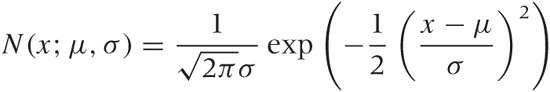
and we seek to estimate values for the parameters (μ and σ this case) from a sample. Note that once we have estimates for the parameters, the distribution describing the population is fully determined, and we can (at least in principle) calculate any desired property of the population directly from that distribution. Parameter estimation comes in two flavors: point estimation and interval estimation. The first just gives us a specific value for the parameter, whereas the second gives us a range of values that is supposed to contain the true value.

Compared with parameter estimation, hypothesis testing is the weirder of the two procedures. It does not attempt to quantify the size of an effect; it merely tries to determine whether there is any effect at all. Note well that this is a largely theoretical argument; from a practical point of view, the existence of an effect cannot be separated entirely from its size. We will come back to this point later, but first let’s understand how hypothesis testing works.

Suppose we have developed a new fertilizer but don’t know yet whether it actually works. Now we run an experiment: we divide a plot of land in two and treat the crops on half of the plot with the new fertilizer. Finally, we compare the yields: are they different? The specific amounts of the yield will almost surely differ, but is this difference due to the treatment or is it merely a chance fluctuation? Hypothesis testing helps us decide how large the difference needs to be in order to be statistically significant.

Formal hypothesis testing now proceeds as follows. First we set up the two hypotheses between which we want to decide: the null hypothesis (no effect; that is there is no difference between the two experiments) and the alternate hypothesis (there is an effect so that the two experiments have significantly different outcomes). If the difference between the outcomes of the two experiments is statistically significant, then we have sufficient evidence to “reject the null hypothesis,” otherwise we “fail to reject the null hypothesis.” In other words: if the outcomes are not sufficiently different, then we retain the null hypothesis that there is no effect.

This convoluted, indirect line of reasoning is required because, strictly speaking, no hypothesis can ever be proved correct by empirical means. If we find evidence against a hypothesis, then we can surely reject it. But if we don’t find evidence against the hypothesis, then we retain the hypothesis—at least until we do find evidence against it (which may possibly never happen, in which case we retain the hypothesis indefinitely).

This, then, is the process by which hypothesis testing proceeds: because we can never prove that a treatment was successful, we instead invent a contradicting statement that we can prove to be false. The price we pay for this double negative (“it’s not true that there is no effect”) is that the test results mean exactly the opposite from what they seem to be saying: “retaining the null hypothesis,” which sounds like a success, means that the treatment had no effect; whereas “rejecting the null hypothesis” means that the treatment did work. This is the first problem with hypothesis testing: it involves a convoluted, indirect line of reasoning and a terminology that seems to be saying the exact opposite from what it means.

But there is another problem with hypothesis testing: it makes a statement that has almost no practical meaning! In reducing the outcome of an experiment to the Boolean choice between “significant” and “not significant,” it creates an artificial dichotomy that is not an appropriate view of reality. Experimental outcomes are not either strictly significant or strictly nonsignificant: they form a continuum. In order to judge the results of an experiment, we need to know where along the continuum the experimental outcome falls and how robust the estimate is. If we have this information, we can decide how to interpret the experimental result and what importance to attach to it.

Classical hypothesis testing exhibits two well-known traps. The first is that an experimental outcome that is marginally outside the statistical significance level abruptly changes the interpretation of the experiment from “significant” to “not significant”—a discontinuity in interpretation that is not borne out by the minimal change in the actual outcome of the experiment. The other problem is that almost any effect, no matter how small, can be made “significant” by increasing the sample size. This can lead to “statistically significant” results that nevertheless are too small to be of any practical importance. All of this is compounded by the arbitrariness of the chosen “significance level” (typically 5 percent). Why not 4.99 percent? Or 1 percent, or 0.1 percent? This seems to render the whole hypothesis testing machinery (at least as generally practiced) fundamentally inconsistent: on the one hand, we introduce an absolutely sharp cutoff into our interpretation of reality; and on the other hand, we choose the position of this cutoff in an arbitrary manner. This does not seem right.

(There is a third trap: at the 5 percent significance level, you can expect 1 out of 20 tests to give the wrong result. This means that if you run enough tests, you will always find one that supports whatever conclusion you want to draw. This practice is known as data dredging and is strongly frowned upon.)

Moreover, in any practical situation, the actual size of the effect is so much more important than its sheer existence. For this reason, hypothesis testing often simply misses the point. A project I recently worked on provides an example of this. The question arose as to whether two events were statistically independent (this is a form of hypothesis testing). But, for the decision that was ultimately made, it did not matter whether the events truly were independent (they were not) but that treating them as independent made no measurable difference to the company’s balance sheet.

Hypothesis testing has its place but typically in rather abstract or theoretical situations where the mere existence of an effect constitutes an important discovery (“Is this coin loaded?” “Are people more likely to die a few days after their birthdays than before?”). If this describes your situation, then you will quite naturally employ hypothesis tests. However, if the size of an effect is of interest to you, then you should feel free to ignore tests altogether and instead work out an estimate of the effect—including its confidence interval. This will give you the information that you need. You are not “doing it wrong” just because you haven’t performed a significance test somewhere along the way.

Finally, I’d like to point out that the statistics community itself has become uneasy with the emphasis that is placed on tests in some fields (notably medicine but also social sciences). Historically, hypothesis testing was invented to deal with sample sizes so small (possibly containing only four or five events) that drawing any conclusion at all was a challenge. In such cases, the broad distinction between “effect” and “no effect” was about the best one could do. If interval estimates are available, there is no reason to use statistical tests. The Wikipedia entry on p-values (explained below) provides some starting points to the controversy.

I have devoted quite a bit of space to a topic that may not seem especially relevant. However, hypothesis tests feature so large in introductory statistics books and courses and, at the same time, are so obscure and counterintuitive, that I found it important to provide some background. In the next section, we will take a more detailed look at some of the concepts and terminology that you are likely to find in introductory (or not-so-introductory) statistics books and courses.

In Chapter 9, we already encountered several well-known probability distributions, including the binomial (used for trials resulting in Success or Failure), the Poisson (applicable in situations where events are evenly distributed according to some density), and the ubiquitous Normal, or Gaussian, distribution. All of these distributions describe real-world, observable phenomena.

In addition, classical statistics uses several distributions that describe the distribution of certain quantities that are not observed but calculated. These distributions are not (or not usually) used to describe events in the real world. Instead, they describe how the outcomes of specific typical calculations involving random quantities will be distributed. There are four of these distributions, and they are known as sampling distributions.

The first of these (and the only one having much use outside of theoretical statistics) is the Gaussian distribution. As a sampling distribution, it is of interest because we already know that it describes the distribution of a sum of independent, identically distributed random variables. In other words, if X₁, X₂,..., X_n are random variables, then Z = X₁ + X₂ + ··· + X_n will be normally distributed and (because we can divide by a constant) the average m = (X₁ + X₂ + ··· + X_n)/n will also follow a Gaussian. It is this last property that makes the Gaussian important as a sampling distribution: it describes the distribution of averages. One caveat: to arrive at a closed formula for the Gaussian, we need to know the variance (i.e., the width) of the distribution from which the individual X_i are drawn. For most practical situations this is not a realistic requirement, and in a moment we will discuss what to do if the variance is not known.

The second sampling distribution is the chi-square (χ²) distribution. It describes the distribution of the sum of squares of independent, identically distributed Gaussian random variables. Thus, if X₁, X₂,..., X_n are Gaussian random variables with unit variance, then 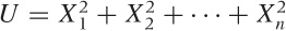will follow a chi-square distribution. Why should we care? Because we form this kind of sum every time we calculate the variance. (Recall that the variance is defined as 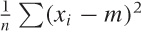.) Hence, the chi-square distribution is used to describe the distribution of variances. The number n of elements in the sum is referred to as the number of degrees of freedom of the chi-square distribution, and it is an additional parameter we need to know to evaluate the distribution numerically.

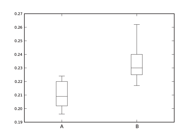
The third sampling distribution describes the behavior of the ratio T of a normally (Gaussian) distributed random variable Z and a chi-square-distributed random variable U. This distribution is the famous Student t distribution. Specifically, let Z be distributed according to the standard Gaussian distribution and U according to the chi-square distribution with n degrees of freedom. Then 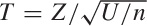is distributed according to the t distribution with n degrees of freedom. As it turns out, this is the correct formula to use for the distribution of the average if the variance is not known but has to be determined from the sample together with the average.

The t distribution is a symmetric, bell-shaped curve like the Gaussian but with fatter tails. How fat the tails are depends on the number of degrees of freedom (i.e., on the number of data points in the sample). As the number of degrees of freedom increases, the t distribution becomes more and more like the Gaussian. In fact, for n larger than about 30, the differences between them are negligible. This is an important point to keep in mind: the distinction between the t distribution and the Gaussian matters only for small samples—that is, samples containing less than approximately 30 data points. For larger samples, it is all right to use the Gaussian instead of the t distribution.

The last of the four sampling distributions is Fisher’s F distribution, which describes the behavior of the ratio of two chi-square random variables. We care about this when we want to compare two variances against each other (e.g., to test whether they are equal or not).

These are the four sampling distributions of classical statistics. I will neither trouble you with the formulas for these distributions, nor show you their graphs—you can find them in every statistics book. What is important here is to understand what they are describing and why they are important. In short, if you have n independent but identically distributed measurements, then the sampling distributions describe how the average, the variance, and their ratios will be distributed. The sampling distributions therefore allow us to reason about averages and variances. That’s why they are important and why statistics books spend so much time on them.

One way to use the sampling distribution is to construct confidence intervals for an estimate. Here is how it works. Suppose we have n observations. We can find the average and variance of these measurements as well as the ratio of the two. Finally, we know that the ratio is distributed according to the t distribution. Hence we can find the interval that has a 95 percent probability of containing the true value (see Figure 10-1). The boundaries of this range are the 95 percent confidence interval; that is, we expect the true value to fall outside this confidence range in only 1 out 20 cases.

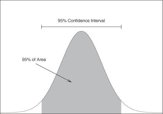
A similar concept can be applied to hypothesis testing, where sampling distributions are often used to calculate so-called p-values. A p-value is an attempt to express the strength of the evidence in a hypothesis test and, in so doing, to soften the sharp binary distinction between significant and not significant outcomes mentioned earlier. A p-value is the probability of obtaining a value as (or more) extreme than the one actually observed under the assumption that the null hypothesis is true (see Figure 10-2). In other words, if the null hypothesis is that there is no effect, and if the observed effect size is x, then the p-value is the probability of observing an effect at least as large as x. Obviously, a large effect is improbable (small p-value) if the null hypothesis (zero effect) is true; hence a small p-value is considered strong evidence against the null hypothesis. However, a p-value is not “the probability that the null hypothesis is true”—such an interpretation (although appealing!) is incorrect. The p-value is the probability of obtaining an effect as large or larger than the observed one if the null hypothesis is true. (Classical statistics does not make probability statements about the truth of hypotheses. Doing so would put us into the realm of Bayesian statistics, a topic we will discuss toward the end of this chapter.)

Figure 10-1. The shaded area contains 95 percent of the area under the curve; the boundaries of the shaded region are the bounds on the 95 percent confidence interval.

By the way, if you are thinking that this approach to hypothesis testing—with its sliding p-values—is quite different from the cut-and-dried significant–not significant approach discussed earlier, then you are right. Historically, two competing theories of significance tests have been developed and have generated quite a bit of controversy; even today they sit a little awkwardly next to each other. (The approach based on sliding p-values that need to be interpreted by the researcher is due to Fisher; the decision-rule approach was developed by Pearson and Neyman.) But enough, already. You can consult any statistics book if you want to know more details.

Figure 10-2. The p-value is the probability of observing a value as large or larger than the one actually observed if the null hypothesis is true.

Example: Formal Tests Versus Graphical Methods

Historically, classical statistics evolved as it did because working with actual data was hard. The early statisticians therefore made a number of simplifying assumptions (mostly that data would be normally distributed) and then proceeded to develop mathematical tools (such as the sampling distributions introduced earlier in the chapter) that allowed them to reason about data sets in a general way and required only the knowledge of a few, easily calculated summary statistics (such as the mean). The ingenuity of it all is amazing, but it has led to an emphasis on formal technicalities as opposed to the direct insight into the data. Today our situation is different, and we should take full advantage of that.

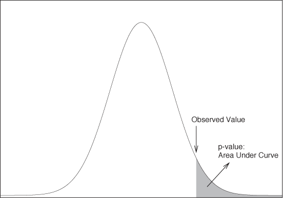
An example will demonstrate what I mean. The listing below shows two data sets. Are they the same, or are they different (in the sense that their means are the same or different)?^[19]

0.209         0.225
0.205         0.262
0.196         0.217
0.210         0.240
0.202         0.230
0.207         0.229
0.224         0.235
0.223         0.217
0.220
0.201

Figure 10-3. Box-and-whisker plots of the two Quintus Curtius Snodgrass data sets. There is almost no overlap between the two.

In case study 9.2.1 of their book, Larsen and Marx (see the recommended reading at the end of this chapter) labor for several pages and finally conclude that the data sets are different at the 99 percent level of significance.

Figure 10-3 shows a box plot for each of the data sets. Case closed.

(In fairness, the formal test does something that a graphical method cannot do: it gives us a quantitative criterion by which to make a decision. I hope that the discussion in this chapter has convinced you that this is not always an advantage, because it can lead to blind faith in “the number.” Graphical methods require you to interpret the results and take responsibility for the conclusions. Which is why I like them: they keep you honest!)

Besides the machinery of formal statistical inference (using the sampling distributions just discussed), the early statistics pioneers also developed a general theory of how best to undertake statistical studies. This conceptual framework is sometimes known as Design of Experiment and is worth knowing about—not least because so much of typical data mining activity does not make use of it.

The most important distinction formalized by the Design of Experiment theory is the one between an observational study and a controlled experiment. As the name implies, a controlled experiment allows us to control many aspects of the experimental setup and procedure; in particular, we control which treatment is applied to which experimental unit (we will define these terms shortly). For example, in an agricultural experiment, we would treat some (but not all) of the plots with a new fertilizer and then later compare the yields from the two treatment groups. In contrast, with an observational study, we merely collect data as it becomes (or already is) available. In particular, retrospective studies are always observational (not controlled).

In a controlled experiment, we are able to control the “input” of an experiment (namely, the application of a treatment) and therefore can draw much more powerful conclusions from the output. In contrast to observational studies, a properly conducted controlled experiment can provide strong support for cause-and-effect relationships between two observations and can be used to rule out hidden (or confounding) causes. Observational studies can merely suggest the existence of a relationship between two observations; however, they can neither prove that one observation is caused by the other nor rule out that additional (unobserved) factors have played a role.

The following (intentionally whimsical) example will serve to make the point. Let’s say we have data that suggests that cities with many lawyers also have many espresso stands and that cities with few lawyers have few espresso stands. In other words, there is strong correlation between the two quantities. But what conclusions can we draw about the causal relationship between the two? Are lawyers particularly high consumers of expensive coffee? Or does caffeine make people more litigious? In short, there is no way for us to determine what is cause and what is effect in this example. In contrast, if the fertilized yields in the controlled agricultural experiment are higher than the yields from the untreated control plots, we have strong reason to conclude that this effect is due to the fertilizer treatment.

In addition to the desire to establish that the treatment indeed causes the effect, we also want to rule out the possibility of additional, unobserved factors that might account for the observed effect. Such factors, which influence the outcome of a study but are not themselves part of it, are known as confounding (or “hidden” or “lurking”) variables. In our agricultural example, differences in soil quality might have a significant influence on the yield—perhaps a greater influence than the fertilizer. The spurious correlation between the number of lawyers and espresso stands is almost certainly due to confounding: larger cities have more of everything! (Even if we account for this effect and consider the per capita density of lawyers and espresso stands, there is still a plausible confounding factor: the income generated per head in the city.) In the next section, we will discuss how randomization can help to remove the effect of confounding variables.

The distinction between controlled experiments and observational studies is most critical. Many of the most controversial scientific or statistical issues involve observational studies. In particular, reports in the mass media often concern studies that (inappropriately) draw causal inferences from observational studies (about topics such as the relationship between gun laws and homicide rates, for example). Sometimes controlled experiments are not possible, with the result that it becomes almost impossible to settle certain questions once and for all. (The controversy around the connection between smoking and lung cancer is a good example.)

In any case, make sure you understand clearly the difference between controlled and observational studies, as well as the fundamental limitations of the latter!

There is an alternative approach to statistics that is based on a different interpretation of the concept of probability itself. This may come as a surprise, since probability seems to be such a basic concept. The problem is that, although we have a very strong intuitive sense of what we mean by the word “probability,” it is not so easy to give it a rigorous meaning that can be used to develop a mathematical theory.

The interpretation of probability used by classical statistics (and, to some degree, by abstract probability theory) treats probability as a limiting frequency: if you toss a fair coin “a large number of times,” then you will obtain Heads about half of the time; hence the probability for Heads is 1/2. Arguments and theories starting from this interpretation are often referred to as “frequentist.”

An alternative interpretation of probability views it as the degree of our ignorance about an outcome: since we don’t know which side will be on top in the next toss of a fair coin, we assign each possible outcome the same probability—namely 1/2. We can therefore make statements about the probabilities associated with individual events without having to invoke the notion of a large number of repeated trials. Because this approach to probability and statistics makes use of Bayes’ theorem at a central step in its reasoning, it is usually called Bayesian statistics and has become increasingly popular in recent years. Let’s compare the two interpretations in a bit more detail.

The Bayesian Interpretation of Probability

To understand the Bayesian point of view, we first need to review the concept of conditional probability. The conditional probability P(A|B) gives us the probability for the event A, given (or assuming) that event B has occurred. You can easily convince yourself that the following is true:

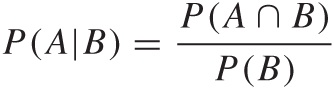
where P(A ∩ B) is the joint probability of finding both event A and event B. For example, it is well known that men are much more likely than women to be color-blind: about 10 percent of men are color-blind but fewer than 1 percent of women are color-blind. These are conditional probabilities—that is, the probability of being color-blind given the gender:

P(color-blind|male) = 0.1

P(color-blind|female) = 0.01

In contrast, if we “randomly” pick a person off the street, then we are dealing with the joint probability that this person is color-blind and male. The person has a 50 percent chance of being male and a 10 percent conditional probability of being color-blind, given that the person is male. Hence, the joint probability for a random person to be color-blind and male is 5 percent, in agreement with the definition of conditional probability given previously.

One can now rigorously prove the following equality, which is known as Bayes’ theorem:

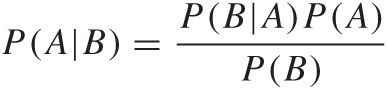
In words: the probability of finding A given B is equal to the probability of finding B given A multiplied by the probability of finding A and divided by the probability of finding B.

Now, let’s return to statistics and data analysis. Assume there is some parameter that we attempt to determine through an experiment (say, the mass of the proton or the survival rate after surgery). We are now dealing with two “events”: event B is the occurrence of the specific set of measurements that we have observed, and the parameter taking some specific value constitutes event A. We can now rewrite Bayes’ theorem as follows:

P(parameter|data) ∝ P(data|parameter)P(parameter)

(I have dropped the denominator, which I can do because the denominator is simply a constant that does not depend on the parameter we wish to determine. The left- and righthand sides are now no longer equal, so I have replaced the equality sign with ∝ to indicate that the two sides of the expression are merely proportional: equal to within a numerical constant.)

Let’s look at this equation term by term.

On the lefthand side, we have the probability of finding a certain value for the parameter, given the data. That’s pretty exciting, because this is an expression that makes an explicit statement about the probability of an event (in this case, that the parameter has a certain value), given the data. This probability is called the posterior probability, or simply the posterior, and is defined solely through Bayes’ theorem without reference to any unlimited sequence of trials. Instead, it is a measure of our “belief” or “certainty” about the outcome (i.e., the value of the parameter) given the data.

The first term on the righthand side, P(data|parameter), is known as the likelihood function. This is a mathematical expression that links the parameter to the probability of obtaining specific data points in an actual experiment. The likelihood function constitutes our “model” for the system under consideration: it tells us what data we can expect to observe, given a particular value of the parameter. (The example in the next section will help to clarify the meaning of this term.)

Finally, the term P(parameter) is known as the prior probability, or simply the prior, and captures our “prior” (prior to the experiment) belief of finding a certain outcome—specifically our prior belief that the parameter has a certain value. It is the existence of this prior that makes the Bayesian approach so controversial, because it seems to introduce an inappropriately subjective element into the analysis. In reality, however, the influence of the prior on the final result of the analysis is typically small, in particular when there is plenty of data. One can also find so-called “noninformative” priors that express our complete ignorance about the possible outcomes. But the prior is there, and it forces us to think about our assumptions regarding the experiment and to state some of these assumptions explicitly (in form of the prior distribution function).

Bayesian Data Analysis: A Worked Example

All of this will become much clearer once we demonstrate these concepts in an actual example. The example is very simple, so as not to distract from the concepts.

Assume we have a coin that has been tossed 10 times, producing the following set of outcomes (H for Heads, T for Tails):

T H H H H T T H H H

If you count the outcomes, you will find that we obtained 7 Heads and 3 Tails in 10 tosses of the coin.

Given this data, we would like to determine whether the coin is fair or not. Specifically, we would like to determine the probability p that a toss of this coin will turn out Heads. (This is the “parameter” we would like to estimate.) If the coin is fair, then p should be close to 1/2.

Let’s write down Bayes’ equation, adapted to this system:

P(p| {T H H H H T T H H H}) ∝ P({T H H H H T T H H H} | p)P(p)

Notice that at this point, the problem has become parametric. All that is left to do is to determine the value of the parameter p or, more precisely, the posterior probability distribution for all values of p.

To make progress, we need to supply the likelihood function and the prior. Given this system, the likelihood function is particularly simple: P(H|p) = p and P(T|p) = 1 – p. You should convince yourself that this choice of likelihood function gives us exactly what we want: the probability to obtain Heads or Tails, given p.

We also assume that the tosses are independent, which implies that only the total number of Heads or Tails matters but not the order in which they occurred. Hence we don’t need to find the combined likelihood for the specific sequence of 10 tosses; instead, the likelihood of the set of events is simply the product of the 10 individual tosses. (The likelihood “factors” for independent events—this argument occurs frequently in Bayesian analysis.)

Figure 10-4. The (unnormalized) posterior probability of obtaining 7 Heads in 10 tosses of a coin as a function of p.

Finally, we know nothing about this coin. In particular, we have no reason to believe that any value of p is more likely than any other, so we choose as prior probability distribution the “flat” distribution P(p) = 1 for all p.

Collecting everything, we end up with the following expression (where I have dropped some combinatorial factors that do not depend on p):

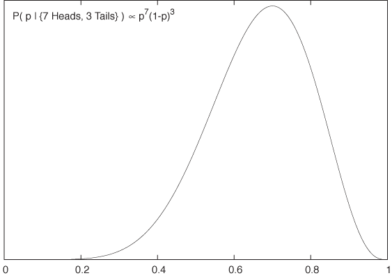
P(p| {7 Heads, 3 Tails}) ∝ p⁷(1 – p)³

This is the posterior probability distribution for the parameter p based on the experimental data (see Figure 10-4). We can see that it has a peak near p = 0.7, which is the most probable value for p. Note that the absence of tick marks on the y axis in Figure 10-4: the denominator, which we dropped earlier, is still undetermined, and therefore the overall scale of the function is not yet fixed. If we are interested only in the location of the maximum, this does not matter.

But we are not restricted to a single (point) estimate for p—the entire distribution function is available to us! We can now use it to construct confidence intervals for p. And because we are now talking about Bayesian probabilities, it would be legitimate to state that “the confidence interval has a 95 percent chance of containing the true value of p.”

We can also evaluate any function that depends on p by integrating it against the posterior distribution for p. As a particularly simple example, we could calculate the expectation value of p to obtain the single “best” estimate of p (rather than use the most probable value as we did before):

Figure 10-5. The (unnormalized) posterior probability of obtaining 70 percent Heads in 10 and in 30 tosses of a coin. The more data there is, the more strongly peaked the posterior distribution becomes.

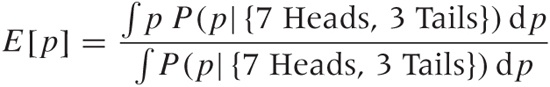
Here we finally need to worry about all the factors that we dropped along the way, and the denominator in the formula is our way of fixing the normalization “after the fact.” To ensure that the probability distribution is properly normalized, we divide explicitly by the integral over the whole range of values, thereby guaranteeing that the total probability equals 1 (as it must).

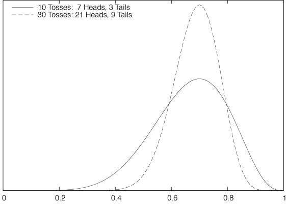
It is interesting to look at the roles played by the likelihood and the prior in the result. In Bayesian analysis, the posterior “interpolates” between the prior and the data-based likelihood function. If there is only very little data, then the likelihood function will be relatively flat, and therefore the posterior will be more influenced by the prior. But as we collect more data (i.e., as the empirical evidence becomes stronger), the likelihood function becomes more and more narrowly peaked at the most likely value of p, regardless of the choice of prior. Figure 10-5 demonstrates this effect. It shows the posterior for a total of 10 trials and a total of 30 trials (while keeping the same ratio of Heads to Tails): as we gather more data, the uncertainty in the resulting posterior shrinks.

Figure 10-6. The effect of a nonflat prior: posterior probabilities for data sets of different sizes, calculated using a Gaussian prior.

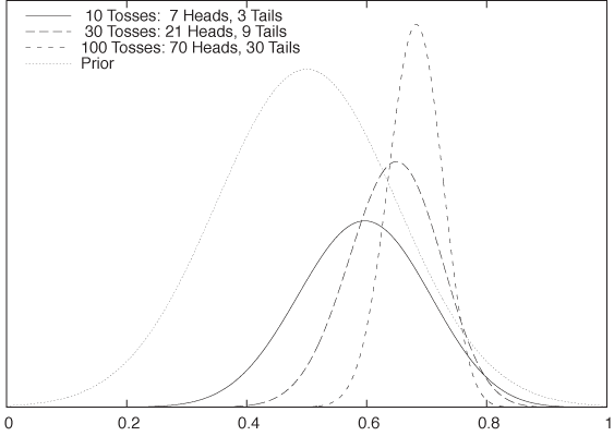
Finally, Figure 10-6 demonstrates the effect of the prior. Whereas the posterior distributions shown in Figure 10-5 were calculated using a flat prior, those in Figure 10-6 were calculated using a Gaussian prior—which expresses a rather strong belief that the value of p will be between 0.35 and 0.65. The influence of this prior belief is rather significant for the smaller data set, but as we take more and more data points, its influence is increasingly diminished.

R is an environment for data manipulation and numerical calculations, specifically statistical applications. Although it can be used in a more general fashion for programming or computation, its real strength is the large number of built-in (or user-contributed) statistical functions.

R is an open source clone of the S programming language, which was originally developed at Bell Labs in the 1970s. It was one of the first environments to combine the capabilities that today we expect from a scripting language (e.g., memory management, proper strings, dynamic typing, easy file handling) with integrated graphics and intended for an interactive usage pattern.

I tend to stress the word environment when referring to R, because the way it integrates its various components is essential to R. It is misleading to think of R as a programming language that also has an interactive shell (like Python or Groovy). Instead, you might consider it as a shell but for handling data instead of files. Alternatively, you might want to view R as a text-based spreadsheet on steroids. The “shell” metaphor in particular is helpful in motivating some of the design choices made by R.

The essential data structure offered by R is the so-called data frame. A data frame encapsulates a data set and is the central abstraction that R is built on. Practically all operations involve the handling and manipulation of frames in one way or the other.

Possibly the best way to think of a data frame is as being comparable to a relational database table. Each data frame is a rectangular data structure consisting of rows and columns. Each column has a designated data type, and all entries in that column must be of that type. Consequently, each row will in general contain entries of different types (as defined by the types of the columns), but all rows must be of the same form. All this should be familiar from relational databases. The similarities continue: operations on frames can either project out a subset of columns, or filter out a subset of rows; either operation results in a new data frame. There is even a command (merge) that can perform a join of two data frames on a common column. In addition (and in contrast to databases), we will frequently add columns to an existing frame—for example, to hold the results of an intermediate calculation.

We can refer to columns by name. The names are either read from the first line of the input file, or (if not provided) R will substitute synthetic names of the form V1, V2, .... In contrast, we filter out a set of rows through various forms of “indexing magic.” Let’s look at some examples.

Consider the following input file:

Name     Height   Weight   Gender
Joe      6.2      192.2    0
Jane     5.5      155.4    1
Mary     5.7      164.3    1
Jill     5.6      166.4    1
Bill     5.8      185.8    0
Pete     6.1      201.7    0
Jack     6.0      195.2    0

Let’s investigate this data set using R, placing particular emphasis on how to handle and manipulate data with R—the full session transcript is included below. The commands entered at the command prompt are prefixed by the prompt >, while R output is shown without the prompt:

> d <- read.csv( "data", header = TRUE, sep = "\t" )
> str(d)
'data.frame':   7 obs. of   4 variables:
 $ Name  : Factor w/ 7 levels "Bill","Jack",..: 5 3 6 4 1 7 2
 $ Height: num  6.2 5.5 5.7 5.6 5.8 6.1 6
 $ Weight: num  192 155 164 166 186 ...
 $ Gender: int  0 1 1 1 0 0 0
>
> mean( d$Weight )
[1] 180.1429
> mean( d[,3] )
[1] 180.1429
>
> mean( d$Weight[ d$Gender == 1 ] )
[1] 162.0333
> mean( d$Weight[ 2:4 ] )
[1] 162.0333
>
> d$Diff <- d$Height - mean( d$Height )
> print(d)
  Name Height Weight Gender        Diff
1  Joe    6.2  192.2      0  0.35714286
2 Jane    5.5  155.4      1 -0.34285714
3 Mary    5.7  164.3      1 -0.14285714
4 Jill    5.6  166.4      1 -0.24285714
5 Bill    5.8  185.8      0 -0.04285714
6 Pete    6.1  201.7      0  0.25714286
7 Jack    6.0  195.2      0  0.15714286
> summary(d)
   Name       Height          Weight          Gender            Diff
  Bill:1  Min.   :5.500   Min.   :155.4   Min.   :0.0000   Min.   :-3.429e-01
  Jack:1  1st Qu.:5.650   1st Qu.:165.3   1st Qu.:0.0000   1st Qu.:-1.929e-01
  Jane:1  Median :5.800   Median :185.8   Median :0.0000   Median :-4.286e-02
  Jill:1  Mean   :5.843   Mean   :180.1   Mean   :0.4286   Mean   : 2.538e-16
  Joe :1  3rd Qu.:6.050   3rd Qu.:193.7   3rd Qu.:1.0000   3rd Qu.: 2.071e-01
  Mary:1  Max.   :6.200   Max.   :201.7   Max.   :1.0000   Max.   : 3.571e-01
  Pete:1
>
> d$Gender <- factor( d$Gender, labels = c("M", "F") )
> summary(d)
    Name      Height          Weight      Gender      Diff
  Bill:1  Min.   :5.500   Min.   :155.4   M:4    Min.   :-3.429e-01
  Jack:1  1st Qu.:5.650   1st Qu.:165.3   F:3    1st Qu.:-1.929e-01
  Jane:1  Median :5.800   Median :185.8          Median :-4.286e-02
  Jill:1  Mean   :5.843   Mean   :180.1          Mean   : 2.538e-16
  Joe :1  3rd Qu.:6.050   3rd Qu.:193.7          3rd Qu.: 2.071e-01
  Mary:1  Max.   :6.200   Max.   :201.7          Max.   : 3.571e-01
  Pete:1
>
> plot( d$Height ~ d$Gender )
> plot( d$Height ~ d$Weight, xlab="Weight", ylab="Height" )

> m <- lm( d$Height ~ d$Weight )
> print(m)

Call:
lm(formula = d$Height ~ d$Weight)

Coefficients:
(Intercept)     d$Weight
    3.39918      0.01357

> abline(m)
> abline( mean(d$Height), 0, lty=2 )

Let’s step through this session in some detail and explain what is going on.

First, we read the file in and assign it to the variable d, which is a data frame as discussed previously. The function str(d) shows us a string representation of the data frame. We can see that the frame consists of five named columns, and we can also see some typical values for each column. Notice that R has assigned a data type to each column: height and weight have been recognized as floating-point values; the names are considered a “factor,” which is R’s way of indicating a categorical variable; and finally the gender flag is interpreted as an integer. This is not ideal—we will come back to that.

> d <- read.csv( "data", header = TRUE, sep = "\t" )
> str(d)
'data.frame':    7 obs. of  4 variables:
 $ Name  : Factor w/ 7 levels "Bill","Jack",..: 5 3 6 4 1 7 2
 $ Height: num  6.2 5.5 5.7 5.6 5.8 6.1 6
 $ Weight: num  192 155 164 166 186 ...
 $ Gender: int  0 1 1 1 0 0 0

Let’s calculate the mean of the weight column to demonstrate some typical ways in which we can select rows and columns. The most convenient way to specify a column is by name: d$Weight. The use of the dollar-sign ($) to access members of a data structure is one of R’s quirks that one learns to live with. Think of a column as a shell variable! (By contrast, the dot (.) is not an operator and can be part of a variable or function name—in the same way that an underscore (_) is used in other languages. Here again the shell metaphor is useful: recall that shells allow the dot as part of filenames!)

> mean( d$Weight )
[1] 180.1429
> mean( d[,3] )
[1] 180.1429

Although its name is often the most convenient method to specify a column, we can also use its numeric index. Each element in a data frame can be accessed using its row and column index via the familiar bracket notation: d[row,col]. Keep in mind that the vertical (row) index comes first, followed by the horizontal (column) index. Omitting one of them selects all possible values, as we do in the listing above: d[,3] selects all rows from the third column. Also note that indices in R start at 1 (mathematical convention), not at 0 (programming convention).

Now that we know how to select a column, let’s see how to select rows. In R, this is usually done through various forms of “indexing magic,” two examples of which are shown next in the listing. We want to find the mean weight of only the women in the sample. To do so, we take the weight column but now index it with a logical expression. This kind of operation takes some getting used to: inside the brackets, we seem to compare a column (d$Gender) with a scalar—and then use the result to index another column. What is going on here? Several things: first, the scalar on the righthand side of the comparison is expanded into a vector of the same length as the operator on the lefthand side. The result of the equality operator is then a Boolean vector of the same length as d$Gender or d$Weight. A Boolean vector of the appropriate length can be used as an index and selects only those rows for which it evaluates as True—which it does in this case only for the women in the sample. The second line of code is much more conventional: the colon operator (:) creates a range of numbers, which are used to index into the d$Weight column. (Remember that indices start at 1, not at 0!)

> mean( d$Weight[ d$Gender == 1 ] )
[1] 162.0333
> mean( d$Weight[ 2:4 ] )
[1] 162.0333

These kinds of operation are very common in R: using some form of creative indexing to filter out a subset of rows (there are more ways to do this, which I don’t show) and mixing vectors and scalars in expressions. Here is another example:

> d$Diff <- d$Height - mean( d$Height )

Here we create an additional column, called d$Diff, as the residual that remains when the mean height is subtracted from each individual’s height. Observe how we mix a column with a scalar expression to obtain another vector.

summary(d)

Next, we calculate the summary of the entire data frame with the new column added. Take a look at the gender column: because R interpreted the gender flag as an integer, it went ahead and calculated its “mean” and other quantities. This is meaningless, of course; the values in this column should be treated as categorical. This can be achieved using the factor() function, which also allows us to replace the uninformative numeric labels with more convenient string labels.

> d$Gender <- factor( d$Gender, labels = c("M", "F") )

As you can see when we run summary(d) again, R treats categorical variables differently: it counts how often each value occurs in the data set.

Finally, let’s take a look at R’s plotting capabilities. First, we plot the height “as a function of” the gender. (R uses the tilde (~) to separate control and response variables; the response variable is always on the left.)

> plot( d$Height ~ d$Gender )

Figure 10-7. A box plot, showing the distribution of heights by gender.

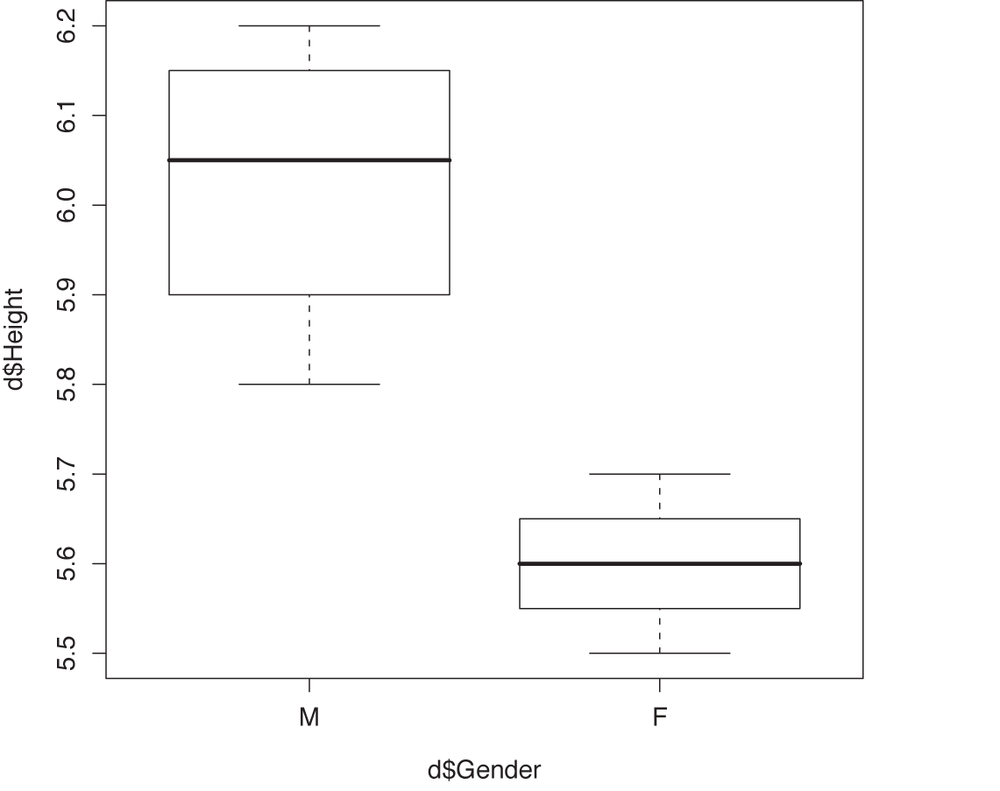
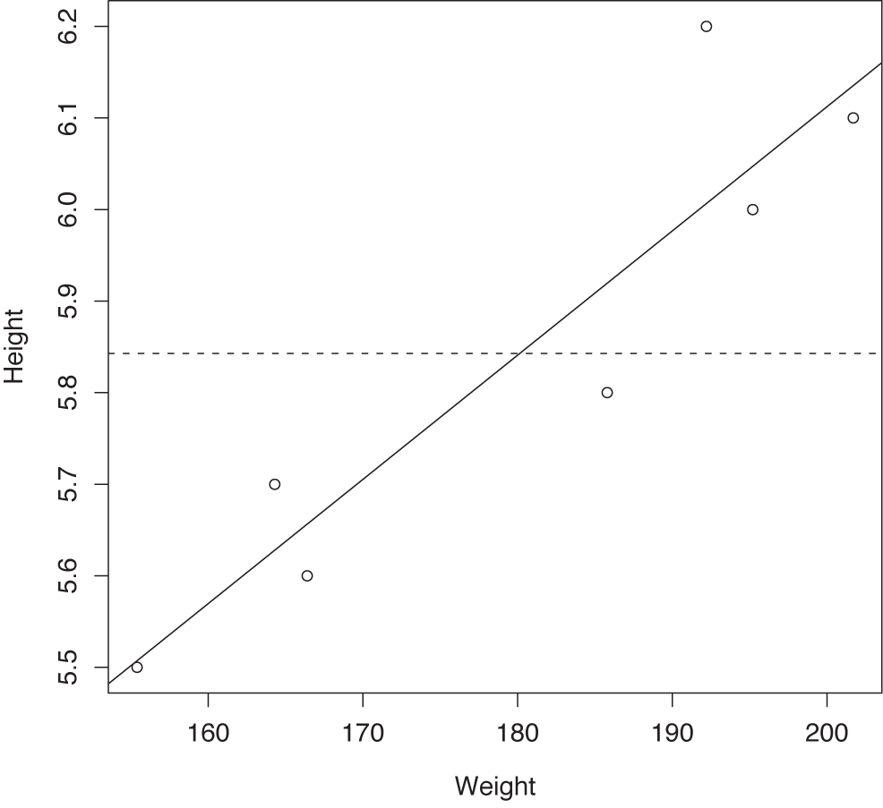
This gives us a box plot, which is shown in Figure 10-7. On the other hand, if we plot the height as a function of the weight, then we obtain a scatter plot (see Figure 10-8—without the lines; we will add them in a moment).

> plot( d$Height ~ d$Weight, xlab="Weight", ylab="Height" )

Given the shape of the data, we might want to fit a linear model to it. This is trivially easy to do in R—it’s a single line of code:

> m <- lm( d$Height ~ d$Weight )

Notice once again the tilde notation used to indicate control and response variable.

We may also want to add the linear model to the scatter plot with the data. This can be done using the abline() function, which plots a line given its offset (“a”) and slope (“b”). We can either specify both parameters explicitly, or simply supply the result m of the fitting procedure; the abline function can use either. (The parameter lty selects the line type.)

> abline(m)
> abline( mean(d$Height), 0, lty=2 )

This short example should have given you an idea of what working with R is like.

R can be difficult to learn: it uses some unfamiliar idioms (such as creative indexing) as well as some obscure function and parameter names. But the greatest challenge to the newcomer (in my opinion) is its indiscriminate use of function overloading. The same function can behave quite differently depending on the (usually opaque) type of inputs it is given. If the default choices made by R are good, then this can be very convenient, but it can be hellish if you want to exercise greater, manual control.

Figure 10-8. A scatter plot with a linear fit.

Look at our example again: the same plot() command generates entirely different plot types depending on whether the control variable is categorical or numeric (box plot in the first case, scatter plot in the latter). For the experienced user, this kind of implicit behavior is of course convenient, but for the beginner, the apparent unpredictability can be very confusing. (In Chapter 14, we will see another example, where the same plot() command generates yet a different type of plot.)

These kinds of issues do not matter much if you use R interactively because you see the results immediately or, in the worst case, get an error message so that you can try something else. However, they can be unnerving if you approach R with the mindset of a contemporary programmer who prefers for operations to be explicit. It can also be difficult to find out which operations are available in a given situation. For instance, it is not at all obvious that the (opaque) return type of the lm() function is admissible input to the abline() function—it certainly doesn’t look like the explicit set of parameters used in the second call to abline(). Issues of this sort make it hard to predict what R will do at any point, to develop a comprehensive understanding of its capabilities, or how to achieve a desired effect in a specific situation.

The number of introductory statistics texts seems almost infinite—which makes it that much harder to find good ones. Below are some texts that I have found useful: