Table of Contents for
Data Analysis with Open Source Tools
 Data Analysis with Open Source Tools
Published by
O'Reilly Media, Inc., 2010
Data Analysis with Open Source Tools
Published by
O'Reilly Media, Inc., 2010
- Cover
- Data Analysis with Open Source Tools
- O'Reilly Strata Conference
- Data Analysis with Open Source Tools
- Dedication
- A Note Regarding Supplemental Files
- Preface
- 1. Introduction
- I. Graphics: Looking at Data
- 2. A Single Variable: Shape and Distribution
- 3. Two Variables: Establishing Relationships
- 4. Time As a Variable: Time-Series Analysis
- 5. More Than Two Variables: Graphical Multivariate Analysis
- 6. Intermezzo: A Data Analysis Session
- II. Analytics: Modeling Data
- 7. Guesstimation and the Back of the Envelope
- 8. Models from Scaling Arguments
- 9. Arguments from Probability Models
- 10. What You Really Need to Know About Classical Statistics
- 11. Intermezzo: Mythbusting—Bigfoot, Least Squares, and All That
- III. Computation: Mining Data
- 12. Simulations
- 13. Finding Clusters
- 14. Seeing the Forest for the Trees: Finding Important Attributes
- 15. Intermezzo: When More Is Different
- IV. Applications: Using Data
- 16. Reporting, Business Intelligence, and Dashboards
- 17. Financial Calculations and Modeling
- 18. Predictive Analytics
- 19. Epilogue: Facts Are Not Reality
- A. Programming Environments for Scientific Computation and Data Analysis
- B. Results from Calculus
- C. Working with Data
- D. About the Author
- Index
- About the Author
- Colophon
- Copyright
Chapter 12. Simulations
IN THIS CHAPTER, WE LOOK AT SIMULATIONS AS A WAY TO UNDERSTAND DATA. IT MAY SEEM STRANGE TO FIND simulations included in a book on data analysis: don’t simulations just generate even more data that needs to be analyzed? Not necessarily—as we will see, simulations in the form of resampling methods provide a family of techniques for extracting information from data. In addition, simulations can be useful when developing and validating models, and in this way, they facilitate our understanding of data. Finally, in the context of this chapter we can take a brief look at a few other relevant topics, such as discrete event simulations and queueing theory.
A technical comment: I assume that your programming environment includes a random-number generator—not only for uniformly distributed random numbers but also for other distributions (this is a pretty safe bet). I also assume that this random-number generator produces random numbers of sufficiently high quality. This is probably a reasonable assumption, but there’s no guarantee: although the theory of random-number generators is well understood, broken implementations apparently continue to ship. Most books on simulation methods will contain information on random-number generators—look there if you feel that you need more detail.
A Warm-Up Question
As a warm-up to demonstrate how simulations can help us analyze data, consider the following example. We are given a data set with the results of eight tosses of a coin: six Heads and two Tails. Given this data, would we say the coin is biased?
The problem is that the data set is small—if there had been 80,000 tosses of which 60,000 came out Heads, then we would have no doubt that the coin was biased. But with just eight tosses, it seems plausible that the imbalance in the results might be due to chance alone—even with a fair coin.
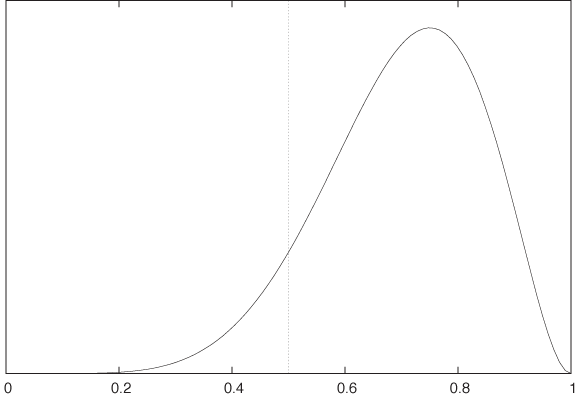
It was for precisely this kind of question that formal statistical methods were developed. We could now either invoke a classical frequentist point of view and calculate the probability of obtaining six or more Heads in eight tosses of a fair coin (i.e., six or more successes in eight Bernoulli trials with p = 0.5). The probability comes out to 37/256 ≈ 0.14, which is not enough to “reject the null hypothesis (that the coin is fair) at the 5 percent level.” Alternatively, we could adopt a Bayesian viewpoint and evaluate the appropriate likelihood function for the given data set with a noninformative prior (see Figure 12-1). The graph suggests that the coin is not balanced.
But what if we have forgotten how to evaluate either quantity, or (more likely!) if we are dealing with a problem more intricate than the one in this example, so that we neither know the appropriate model to choose nor the form of the likelihood function? Can we find a quick way to make progress on the question we started with?
Given the topic of this chapter, the answer is easy. We can simulate tosses of a coin, for various degrees of imbalance, and then compare the simulation results to our data set.
import random

repeats, tosses = 60, 8
def heads( tosses, p ):
h = 0
for x in range( 0, tosses ):
if random.random() < p: h += 1
return h
p = 0
while p < 1.01:
for t in range( 0, repeats ):
print p, "\t", heads( tosses, p )
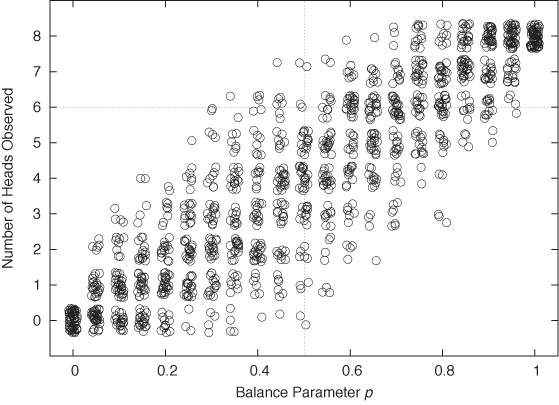
p += 0.05The program is trivial to write, and the results, in the form of a jitter plot, are shown in Figure 12-2. (For each value of the parameter p, which controls the imbalance of the coin, we have performed 60 repeats of 8 tosses each and counted the number of Heads in each repeat.)
The figure is quite clear: for p = 0.5 (i.e., a balanced coin), it is pretty unlikely to obtain six or more Heads, although not at all impossible. On the other hand, given that we have observed six Heads, we would expect the parameter to fall into the range p = 0.6,..., 0.7. We have thus not only answered the question we started with but also given it some context. The simulation therefore not only helped us understand the actual data set but also allowed us to explore the system that produced it. Not bad for 15 lines of code.
Monte Carlo Simulations
The term Monte Carlo simulation is frequently used to describe any method that involves the generation of random points as input for subsequent operations.
Monte Carlo techniques are a major topic all by themselves. Here, I only want to sketch two applications that are particularly relevant in the context of data analysis and modeling. First, simulations allow us to verify analytical work and to experiment with it further; second, simulations are a way of obtaining results from models for which analytical solutions are not available.
Combinatorial Problems
Many basic combinatorial problems can be solved exactly—but obtaining a solution is often difficult. Even when one is able to find a solution, it is surprisingly easy to arrive at incorrect conclusions, missing factors like 1/2 or 1/n! and so on. And lastly, it takes only innocuous looking changes to a problem formulation to render the problem intractable.
In contrast, simulations for typical combinatorial problems are often trivially easy to write. Hence they are a great way to validate theoretical results, and they can be extended to explore problems that are not tractable otherwise.
Here are some examples of questions that can be answered easily in this way:
If we place n balls into n boxes, what is the probability that no more than two boxes contain two or more balls? What if I told you that exactly m boxes are empty? What if at most m boxes are empty?
If we try keys from a key chain containing n different keys, how many keys will we have to try before finding the one that fits the lock? How is the answer different if we try keys randomly (with replacement) as opposed to in order (without replacement)?
Suppose an urn contains 2n tokens consisting of n pairs of items. (Each item is marked in such a way that we can tell to which pair it belongs.) Repeatedly select a single token from the urn and put it aside. Whenever the most recently selected token is the second item from a pair, take both items (i.e., the entire pair) and return them to the urn. How many “broken pairs” will you have set aside on average? How does the answer change if we care about triples instead of pairs? What fluctuations can we expect around the average value?
The last problem is a good example of the kind of problem for which the simple case (average number of broken pairs) is fairly easy to solve but that becomes rapidly more complicated as we make seemingly small modifications to the original problem (e.g., going from pairs to triples). However, in a simulation such changes do not pose any special difficulties.
Another way that simulations can be helpful concerns situations that appear unfamiliar or even paradoxical. Simulations allow us to see how the system behaves and thereby to develop intuition for it. We already encountered an example in the Workshop section of Chapter 9, where we studied probability distributions without expectation values. Let’s look at another example.
Suppose, we are presented with a choice of three closed envelopes. One envelope contains a prize, the other two are empty. After we have selected an envelope, it is revealed that one of the envelopes that we had not selected is empty. We are now permitted to choose again. What should we do? Stick with our initial selection? Randomly choose between the two remaining envelopes? Or pick the remaining envelope—that is, not the one that we selected initially and not the one that has been opened?
This is a famous problem, which is sometimes known as the “Monty Hall Problem” (after the host of a game show that featured a similar game).
As it turns out, the last strategy (always switch to the remaining envelope) is the most beneficial. The problem appears to be paradoxical because the additional information that is revealed (that an envelope we did not select is empty) does not seem to be useful in any way. How can this information affect the probability that our initial guess was correct?
The argument goes as follows. Our initial selection is correct with probability p = 1/3 (because one envelope among the original three contains the prize). If we stick with our original choice, then we should therefore have a 33 percent chance of winning. On the other hand, if in our second choice, we choose randomly from the remaining options (meaning that we are as likely to pick the initially chosen envelope or the remaining one), then we will select the correct envelope with probability p = 1/2 (because now one out of two envelopes contains the prize). A random choice is therefore better than staying put!
But this is still not the best strategy. Remember that our initial choice only had a p = 1/3 probability of being correct—in other words, it has probability q = 2/3 of being wrong. The additional information (the opening of an empty envelope) does not change this probability, but it removes all alternatives. Since our original choice is wrong with probability q = 2/3 and since now there is only one other envelope remaining, switching to this remaining envelope should lead to a win with 66 percent probability!
I don’t know about you, but this is one of those cases where I had to “see it to believe it.” Although the argument above seems compelling, I still find it hard to accept. The program in the following listing helped me do exactly that.
  import sys
  import random as rnd

  strategy = sys.argv[1]  # must be 'stick', 'choose', or 'switch'

  wins = 0
  for trial in range( 1000 ):

  # The prize is always in envelope 0 ... but we don't know that!
  envelopes = [0, 1, 2]

  first_choice = rnd.choice( envelopes )

  if first_choice == 0:
      envelopes = [0, rnd.choice( [1,2] ) ] # Randomly retain 1 or 2
  else:
      envelopes = [0, first_choice] # Retain winner and first choice

  if strategy == 'stick':
      second_choice = first_choice
  elif strategy == 'choose':
      second_choice = rnd.choice( envelopes )
  elif strategy == 'switch':
      envelopes.remove( first_choice )
      second_choice = envelopes[0]

  # Remember that the prize is in envelope 0
  if second_choice == 0:
      wins += 1

print wins
The program reads our strategy from the command line:
the possible choices are stick,
choose, and switch. It then performs a thousand trials
of the game. The “prize” is always in envelope 0, but we don’t know that. Only if our
second choice equals envelope 0
we count the game as a win.
The results from running this program are consistent with the
argument given previously: stick
wins in one third of all trials, choose wins half the time, but switch amazingly wins in two thirds of all
cases.
Obtaining Outcome Distributions
Simulations can be helpful to verify with combinatorial problems, but the primary reason for using simulations is that they allow us to obtain results that are not available analytically. To arrive at an analytical solution for a model, we usually have to make simplifying assumptions. One particularly common one is to replace all random quantities with their most probable value (the mean-field approximation; see Chapter 8). This allows us to solve the model, but we lose information about the distribution of outcomes. Simulations are a way of retaining the effects of randomness when determining the consequences of a model.
Let’s return to the case study discussed at the end of Chapter 9. We had a visitor population making visits to a certain website. Because individual visitors can make repeat visits, the number of unique visitors grows more slowly than the number of total visitors. We found an expression for the number of unique visitors over time but had to make some approximations in order to make progress. In particular, we assumed that the number of total visitors per day would be the same every day, and be equal to the average number of visitors per day. (We also assumed that the fraction of actual repeat visitors on any given day would equal the fraction of repeat visitors in the total population.)
Both of these assumptions are of precisely the nature discussed earlier: we replaced what in reality is a random quantity with its most probable value. These approximations made the problem tractable, but we lost all sense of the accuracy of the result. Let’s see how simulations can help provide additional insight to this situation.
The solution which in Chapter 9 was a
model: an analytical (mean-field) model. The
short program that follows is another model of the same system, but
this time it is a simulation model. It is a
model in the sense that again everything that is not absolutely
essential has been stripped away: there is no website, no actual
visits, no browsing behavior. But the model retains two aspects that
are important and that were missing from the mean-field model.
First, the number of visitors per day is no longer fixed, instead it
is distributed according to a Gaussian distribution. Second, we have
a notion of individual visitors (as elements of the list has_visited), and on every “day” we make a
random selection from this set of visitors to determine who does
visit on this day and who does not.
import random as rnd

n = 1000    # total visitors
k = 100     # avg visitors per day
s = 50      # daily variation

def trial():
    visitors_for_day = [0]  # No visitors on day 0

    has_visited = [0]*n     # A flag for each visitor
    for day in range( 31 ):
        visitors_today = max( 0, int(rnd.gauss( k, s )) )

        # Pick the individuals who visited today and mark them
        for i in rnd.sample( range( n ), visitors_today ):
            has_visited[i] = 1

        # Find the total number of unique visitors so far
        visitors_for_day.append( sum(has_visited) )

return visitors_for_day


for t in range( 25 ):
    r = trial()
    for i in range( len(r) ):
        print i, r[i]

    print
    print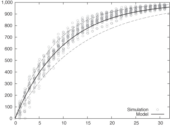
The program performs 25 trials, where each trial consists of a full, 31-day month of visits. For each day, we find the number of visitors for that day (which must be a positive integer) and then randomly select the same number of “visitors” from our list of visitors, setting a flag to indicate that they have visited. Finally, we count the number of visitors that have the flag set and print this number (which is the number of unique visitors so far) for each day. The results are shown in Figure 12-3.
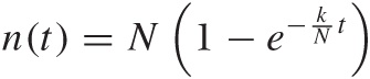
Figure 12-3 also includes results from the analytical model. In Chapter 9, we found that the number of unique visitors on day t was given by:
where N is the total number of visitors
(N = 1,000 in the simulation) and
k is the average number of visitors per day
(k = 100 in the simulation). Accordingly, the
solid line in Figure 12-3 is given by
n(t) = 1,000
 .
.
The simulation includes a parameter that was not part of the analytical model—namely the width s of the daily fluctuations in visitors. I have chosen the value s = 50 for the simulation runs. The dashed lines in Figure 12-3 show the analytical model, with values of k ± s/2 (i.e., k = 75 and k = 125) to provide a sense for the predicted spread, according to the mean-field model.
First of all, we should note that the analytical model agrees very well with the data from the simulation run: that’s a nice confirmation of our previous result! But we should also note the differences; in particular, the simulation results are consistently higher than the theoretical predictions. If we think about this for a moment, this makes sense. If on any day there are unusually many visitors, then this irrevocably bumps the number of unique visitors up: the number of unique visitors can never shrink, so any outlier above the average can never be neutralized (in contrast to an outlier below the average, which can be compensated by any subsequent high-traffic day).
We can further analyze the data from the simulation run, depending on our needs. For instance, we can calculate the most probable value for each day, and we can estimate proper confidence intervals around it. (We will need more than 25 trials to obtain a good estimate of the latter.)
What is more interesting about the simulation model developed here is that we can use it to obtain additional information that would be difficult or impossible to calculate from the analytical formula. For example, we may ask for the distribution of visits per user (i.e., how many users have visited once, twice, three times, and so on). The answer to this question is just a snap of the fingers away! We can also extend the model and ask for the number of unique visitors who have paid two or more visits (not just one). (For two visits per person, this question can be answered within the framework of the original analytical model, but the calculations rapidly become more tedious as we are asking for higher visit counts per person.)
Finally, we can extend the simulation to include features not included in the analytical model at all. For instance, for a real website, not all possible visitors are equally likely to visit: some individuals will have a higher probability of visiting the website than do others. It would be very difficult to incorporate this kind of generalization into the approach taken in Chapter 9, because it contradicts the basic assumption that the fraction of actual repeat visitors equals the fraction of repeat visitors in the total population. But it is not at all difficult to model this behavior in a simulation model!
Pro and Con
Basic simulations of the kind discussed in this section are often easy to program—certainly as compared with the effort required to develop nontrivial combinatorial arguments! Moreover, when we start writing a simulation project, we can be fairly certain of being successful in the end; whereas there is no guarantee that an attempt to find an exact answer to a combinatorial problem will lead anywhere.
On the other hand, we should not forget that a simulation produces numbers, not insight! A simulation is always only one step in a larger process, which must include a proper analysis of the results from the simulation run and, ideally, also involves an attempt to incorporate the simulation data into a larger conceptual model. I always get a little uncomfortable when presented with a bunch of simulation results that have not been fit into a larger context. Simulations cannot replace analytical modeling.
In particular, simulations do not yield the kind of insight into the mechanisms driving certain developments that a good analytical model affords. For instance, recall the case study near the end of Chapter 8, in which we tried to determine the optimal number of servers. One important insight from that model was that the probability pn for a total failure dropped extremely rapidly as the number n of servers increased: the exponential decay (with n) is much more important than the reliability p of each individual server. (In other words, redundant commodity hardware beats expensive supercomputers—at least for situations in which this simplified cost model holds!) This is the kind of insight that would be difficult to gain simply by looking at results from simulation runs.
Simulations can be valuable for verifying analytical work and for extending it by incorporating details that would be difficult or impossible to treat in an analytical model. At the same time, the benefit that we can derive from simulations is enhanced by the insight gained from the analytical, conceptual modeling of the the mechanisms driving a system.
The two methods are complementary—although I will give primacy to analytical work. Analytical models without simulation may be crude but will still yield insight, whereas simulations without analysis produce only numbers, not insight.
Resampling Methods
Imagine you have taken a sample of n points from some population. It is now a trivial exercise to calculate the mean from this sample. But how reliable is this mean? If we repeatedly took new samples (of the same size) from the population and calculated their means, how much would the various values for the mean jump around?
This question is important. A point estimate (such as the mean by itself) is not very powerful: what we really want is an interval estimate which also gives us a sense of the reliability of the answer.
If we could go back and draw additional samples, then we could obtain the distribution of the mean directly as a histogram of the observed means. But that is not an option: all we have are the n data points of the original sample.
Much of classical statistics deals with precisely this question: how can we make statements about the reliability of an estimate based only on a set of observations? To make progress, we need to make some assumptions about the way values are distributed. This is where the sampling distributions of classical statistics come in: all those Normal, t, and chi-square distributions (see Chapter 10). Once we have a theoretical model for the way points are distributed, we can use this model to establish confidence intervals.
Being able to make such statements is one of the outstanding achievements of classical statistics, but at the same time, the difficulties in getting there are a major factor in making classical statistics seem so obscure. Two problems stand out:
Our assumptions about the shape of those distributions may not be correct, or we may not be able to formulate those distributions at all—in particular, if we are interested in more complicated quantities than just the sample mean or if we are dealing with populations that are ill behaved (i.e., not even remotely Gaussian).
Even if we know the sampling distribution, determining confidence limits from it may be tedious, opaque, and error-prone.
The Bootstrap
The bootstrap is an alternative approach for finding confidence intervals and similar quantities directly from the data. Instead of making assumptions about the distribution of values and then employing theoretical arguments, the bootstrap goes back to the original idea: what if we could draw additional samples from the population?
We can’t go back to the original population, but the sample that we already have should be a fairly good approximation to the overall population. We can therefore create additional samples (also of size n) by sampling with replacement from the original sample. For each of these “synthetic” samples, we can calculate the mean (or any other quantity, of course) and then use this set of values for the mean to determine a measure of the spread of its distribution via any standard method (e.g., we might calculate its inter-quartile range; see Chapter 2).
Let’s look at an example—one that is simple enough that we can
work out the analytical answer and compare it directly to the
bootstrap results. We draw n = 25 points from a
standard Gaussian distribution (with mean μ = 0 and standard
deviation σ = 1). We then ask about the (observed) sample mean and
more importantly, about its standard error. In this case, the answer
is simple: we know that the error of the mean is  (see Chapter 11), which
amounts to 1/5 here. This is the analytical result.
(see Chapter 11), which
amounts to 1/5 here. This is the analytical result.
To find the bootstrap estimate for the standard error, we draw 100 samples, each containing n = 25 points, from our original sample of 25 points. Points are drawn randomly with replacement (so that each point can be selected multiple times). For each of these bootstrap samples, we calculate the mean. Now we ask: what is the spread of the distribution of these 100 bootstrap means?
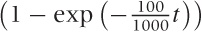
The data is plotted in Figure 12-4. At the bottom, we see the 25 points of the original data sample; above that, we see the means calculated from the 100 bootstrap samples. (All points are jittered vertically to minimize overplotting.) In addition, the figure shows kernel density estimates (see Chapter 2) of the original sample and also of the bootstrap means. The latter is the answer to our original question: if we repeatedly took samples from the original distribution, the sample means would be distributed similarly to the bootstrap means.
(Because in this case we happen to know the original
distribution, we can also plot both it and the theoretical
distribution of the mean, which happens to be Gaussian as well but
with a reduced standard deviation of . As we would expect, the theoretical
distributions agree reasonably well with the kernel density
estimated calculated from the data.)
Of course, in this example the bootstrap procedure was not necessary. It should be clear, however, that the bootstrap provides a simple method for obtaining confidence intervals even in situations where theoretical results are not available. For instance, if the original distribution had been highly skewed, then the Gaussian assumption would have been violated. Similarly, if we had wanted to calculate a more complicated quantity than the mean, analytical results might have been hard to obtain.
Let me repeat this, because it’s important: bootstrapping is a method to estimate the spread of some quantity. It is not a method to obtain “better” estimates of the original quantity itself—for that, it is necessary to obtain a larger sample by making additional drawings from the original population. The bootstrap is not a way to give the appearance of a larger sample size by reusing points!
When Does Bootstrapping Work?
As we have seen, the bootstrap is a simple, practical, and relatively transparent method to obtain confidence intervals for estimated quantities. This begs the question: when does it work? The following two conditions must be fulfilled.
The original sample must provide a good representation of the entire population.
The estimated quantity must depend “smoothly” on the data points.
The first condition requires the original sample to be sufficiently large and relatively clean. If the sample size is too small, then the original estimate for the actual quantity in question (the mean, in our example) won’t be very good. (Bootstrapping in a way exacerbates this problem because data points have a greater chance of being reused repeatedly in the bootstrap samples.) In other words, the original sample has to be large enough to allow meaningful estimation of the primary quantity. Use common sense and insight into your specific application area to establish the required sample size for your situation.
Additionally, the sample has to be relatively clean: crazy outliers, for instance, can be a problem. Unless the sample size is very large, outliers have a significant chance of being reused in a bootstrap sample, distorting the results.
Another problem exists in situations involving power-law distributions. As we saw in Chapter 9, estimated values for such distributions may not be unique but depend on the sample size. Of course, the same considerations apply to bootstrap samples drawn from such distributions.
The second condition suggests that bootstrapping does not work well for quantities that depend critically on only a few data points. For example, we may want to estimate the maximum value of some distribution. Such an estimate depends critically on the largest observed value—that is, on a single data point. For such applications, the bootstrap is not suitable. (In contrast, the mean depends on all data points and with equal weight.)
Another questions concerns the number of bootstrap samples to take. The short answer is: as many as you need to obtain a sufficiently good estimate for the spread you are calculating. If the number of points in the original sample is very small, then creating too many bootstrap samples is counterproductive because you will be regenerating the same bootstrap samples over and over again. However, for reasonably sized samples, this is not much of a problem, since the number of possible bootstrap samples grows very quickly with the number of data points n in the original sample. Therefore, it is highly unlikely that the same bootstrap example is generated more than once—even if we generate thousands of bootstrap samples.
The following argument will help to develop a sense for the order of magnitudes involved. The problem of choosing n data points with replacement from the original n-point sample is equivalent to assigning n elements to n cells. It is a classical problem in occupancy theory to show that there are:

ways of doing this. This number grows extremely quickly: for n = 5 it is 126, for n = 10 we have 92,378, but for n = 20 it already exceeds 1010.
(The usual proof proceeds by observing that assigning
r indistinguishable objects to
n bins is equivalent to aligning
r objects and n – 1 bin
dividers. There are r + n
– 1 spots in total, which can be occupied by either an object or a
divider, and the assignment amounts to choosing
r of these spots for the r
objects. The number of ways one can choose r
elements out of n + r – 1
is given by the binomial coefficient  . Since in our case r =
n, we find that the number of different
bootstrap samples is given by the expression above.)
. Since in our case r =
n, we find that the number of different
bootstrap samples is given by the expression above.)
Bootstrap Variants
There are a few variants of the basic bootstrap idea. The method so far—in which points are drawn directly from the original sample—is known as the nonparametric bootstrap. An alternative is the parametric bootstrap: in this case, we assume that the original population follows some particular probability distribution (such as the Gaussian), and we estimate its parameters (mean and standard deviation, in this case) from the original sample. The bootstrap samples are then drawn from this distribution rather than from the original sample. The advantage of the parametric bootstrap is that the bootstrap values do not have to coincide exactly with the known data points. In a similar spirit, we may use the original sample to compute a kernel density estimate (as an approximation to the population distribution) and then draw bootstrap samples from it. This method combines aspects of both parametric and nonparametric approaches: it is nonparametric (because it make no assumption about the form of the underlying population distribution), yet the bootstrap samples are not restricted to the values occurring in the original sample. In practice, neither of these variants seems to provide much of an advantage over the original idea (in part because the number of possible bootstrap samples grows so quickly with the number of points in the sample that choosing the bootstrap samples from only those points is not much of a restriction).
Another idea (which historically predates the bootstrap) is the so-called jackknife. In the jackknife, we don’t draw random samples. Instead, given an original sample consisting of n data points, we calculate the n estimates of the quantity of interest by successively omitting one of the data points from the sample. We can now use these n values in a similar way that we used values calculated from bootstrap samples. Since the jackknife does not contain any random element, it is an entirely deterministic procedure.
Workshop: Discrete Event Simulations with SimPy
All the simulation examples that we considered so far were either static (coin tosses, Monty Hall problem) or extremely stripped down and conceptual (unique visitors). But if we are dealing with the behavior and time development of more complex systems—consisting of many different particles or actors that interact with each other in complicated ways—then we want a simulation that expresses all these entities in a manner that closely resembles the problem domain. In fact, this is probably exactly what most of us think of when we hear the term “simulation.”
There are basically two different ways that we can set up such a simulation. In a continuous time simulation, time progresses in “infinitesimally” small increments. At each time step, all simulation objects are advanced while taking possible interactions or status changes into account. We would typically choose such an approach to simulate the behavior of particles moving in a fluid or a similar system.
But in other cases, this model seems wasteful. For instance, consider customers arriving at a bank: in such a situation, we only care about the events that change the state of the system (e.g., customer arrives, customer leaves)—we don’t actually care what the customers do while waiting in line! For such system we can use a different simulation method, known as discrete event simulation. In this type of simulation, time does not pass continuously; instead, we determine when the next event is scheduled to occur and then jump ahead to exactly that moment in time.
Discrete event simulations are applicable to a wide variety of problems involving multiple users competing for access to a shared server. It will often be convenient to phrase the description in terms of the proverbial “customers arriving at a bank,” but exactly the same considerations apply, for instance, to messages on a computer network.
Introducing SimPy
The SimPy package (http://simpy.sourceforge.net/) is a Python project to build discrete event simulation models. The framework handles all the event scheduling and messaging “under the covers” so that the programmer can concentrate on describing the behavior of the actors in the simulation.
All actors in a SimPy simulation must be subclasses of the
class Process. Congestion points
where queues form are modeled by instances of the Resource class or its subclasses. Here is
a short example, which describes a customer visiting a bank:
from SimPy.Simulation import *

class Customer( Process ):
    def doit( self ):
        print "Arriving"
        yield request, self, bank

        print "Being served"
        yield hold, self, 100.0

        print "Leaving"
        yield release, self, bank

# Beginning of main simulation program
initialize()

bank = Resource()

cust = Customer()
cust.start( cust.doit() )

simulate( until=1000 )
Let’s skip the class definition of the Customer object for now and concentrate on
the rest of the program. The first function to call in any SimPy
program is the initialize()
method, which sets up the simulation run and sets the “simulation
clock” to zero. We then proceed to create a Resource object (which models the bank)
and a single Customer object.
After creating the Customer, we
need to activate it via the start() member function. The start() function takes as argument the
function that will be called to advance the Customer through its life cycle (we’ll
come back to that). Finally, we kick off the actual simulation,
requiring it to stop after 1,000 time steps on the simulation clock
have passed.
The Customer subclasses
Process, therefore its instances
are active agents, which will be scheduled by the framework to
receive events. Each agent must define a process execution
method (PEM), which defines its behavior and which will
be invoked by the framework whenever an event occurs.
For the Customer class, the
PEM is the doit() function.
(There are no restrictions on its name—it can be called anything.)
The PEM describes the customer’s behavior: after the customer
arrives, the customer requests a resource
instance (the bank in this case).
If the resource is not available (because it is busy, serving other
customers), then the framework will add the customer to the waiting
list (the queue) for the requested resource.
Once the resource becomes available, the customer is being serviced.
In this simple example, the service time is a fixed value of 100
time units, during which the customer instance is
holding—just waiting until the time has passed.
When service is complete, the customer releases
the resource instance. Since no additional actions are listed in the
PEM, the customer is not scheduled for future events and will
disappear from the simulation.
Notice that the Customer
interacts with the simulation environment through Python yield statements, using special yield
expressions of the form shown in the example. Yielding control back
to the framework in this way ensures that the Customer retains its state and its current
spot in the life cycle between invocations. Although there are no
restrictions on the name and argument list permissible for a PEM,
each PEM must contain at least one of these
special yield statements. (But of
course not necessarily all three, as in this case; we are free to
define the behavior of the agents in our simulations at
will.)
The Simplest Queueing Process
Of course the previous example which involved only a single customer entering and leaving the bank, is not very exciting—we hardly needed a simulation for that! Things change when we have more than one customer in the system at the same time.
The listing that follows is very similar to the previous
example, except that now there is an infinite stream of customers
arriving at the bank and requesting service. To generate this
infinite sequence of customers, the listing makes use of an idiom
that’s often used in SimPy programs: a “source” (the CustomerGenerator instance).
from SimPy.Simulation import *
import random as rnd

interarrival_time = 10.0
service_time = 8.0


class CustomerGenerator( Process ):
    def produce( self, b ):
        while True:
            c = Customer( b )
            c.start( c.doit() )
            yield hold, self, rnd.expovariate(1.0/interarrival_time)


class Customer( Process ):
    def __init__( self, resource ):
        Process.__init__( self )
        self.bank = resource

    def doit( self ):
        yield request, self, self.bank
        yield hold, self, self.bank.servicetime()
        yield release, self, self.bank

class Bank( Resource ):
    def servicetime( self ):
        return rnd.expovariate(1.0/service_time)


initialize()

bank = Bank( capacity=1, monitored=True, monitorType=Monitor )

src = CustomerGenerator()
activate( src, src.produce( bank ) )

simulate( until=500 )


print bank.waitMon.mean()
print

for evt in bank.waitMon:
    print evt[0], evt[1]
The CustomerGenerator is
itself a subclass of Process and
defines a PEM (produce()).
Whenever it is triggered, it generates a new Customer and then goes back to sleep for a
random amount of time. (The time is distributed according to an
exponential distribution—we will discuss this particular choice in a
moment.) Notice that we don’t need to keep track of the Customer instances explicitly: once they
have been activated using the start() member function, the framework
ensures that they will receive scheduled events.
There are two changes to the Customer class. First of all, we
explicitly inject the resource to request (the bank) as an additional argument to the
constructor. By contrast, the Customer in the previous example found the
bank reference via lookup in the
global namespace. That’s fine for small programs but becomes
problematic for larger ones—especially if there is more than one
resource that may be requested. The second change is that the
Customer now asks the
bank for the service time. This is in the
spirit of problem domain modeling—it’s usually the server (in this
case, the bank) that controls the time it takes to complete a
transaction. Accordingly, we have introduced Bank as subclass of Resource in order to accommodate this
additional functionality. (The service time is also exponentially
distributed but with a different wait time than that used for the
CustomerGenerator.)
Subtypes of the Process
class are used to model actors in a SimPy simulation. Besides these
active simulation objects, the next most important abstraction
describes congestion points, modeled by the Resource class and its subclasses. Each
Resource instance models a shared
resource that actors may request, but its more important function is
to manage the queue of actors currently waiting
for access.
Each Resource instance
consists of a single queue and one or more actual “server units”
that can fulfill client requests. Think of the typical queueing
discipline followed in banks and post offices (in the U.S.—other
countries have different conventions!): a single line but multiple
teller windows, with the person at the head of the line moving to
the next available window. That is the model represented by each
Resource instance. The number of
server units is controlled through the keyword argument capacity to the Resource constructor. Note that all server
units in a single Resource
instance are identical. Server units are also “passive”: they have
no behavior themselves. They only exist so that a Process object can acquire them, hold them
for a period of time, and then release them (like a mutex).
Although a Resource
instance may have multiple server units, it can contain only a
single queue. If you want to model a supermarket checkout situation,
where each server unit has its own queue, you therefore need to set
up multiple Resource instances,
each with capacity=1: one for
each checkout stand and each managing its own queue of
customers.
For each Resource instance,
we can monitor the length of the queue and the events that change it
(arrivals and departures) by registering an observer object with the
Resource. There are two types of
such observers in SimPy: a Monitor records the time stamp and new
queue length for every event that affects the queue, whereas a
Tally only keeps enough
information to calculate summary information (such as the average
queue length). Here we have registered a Monitor object with the Bank. (We’ll later see an example of a
Tally.)
As before, we run the simulation until the internal simulation
clock reaches 1,000. The CustomerGenerator produces an infinite
stream of Customer objects, each
requesting service from the Bank,
while the Monitor records all
changes to the queue.
After the simulation has run to completion, we
retrieve the Monitor object from
the Bank: if an observer had been
registered with a Resource, then
it is available in the waitMon
member variable. We print out the average queue length over the
course of the simulation as well as the full time series of events.
(The Monitor class is a List subclass, so we can iterate over it
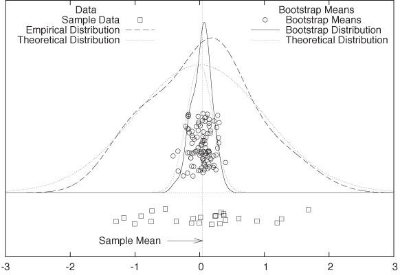
directly.) The time evolution of the queue is shown in Figure 12-5.
One last implementation detail: if you look closely, you will
notice that the CustomerGenerator
is activated using the standalone function activate(). This function is an
alternative to the start() member
function of all Process objects
and is entirely equivalent to it.
Optional: Queueing Theory
Now that we have seen some of these concepts in action already, it is a good time to step back and fill in some theory.
A queue is a specific example of a stochastic process. In general, the term “stochastic process” refers to a sequence of random events occurring in time. In the queueing example, customers are joining or leaving the queue at random times, which makes the queue grow and shrink accordingly. Other examples of stochastic processes include random walks, the movement of stock prices, and the inventory levels in a store. (In the latter case, purchases by customers and possibly even deliveries by suppliers constitute the random events.)
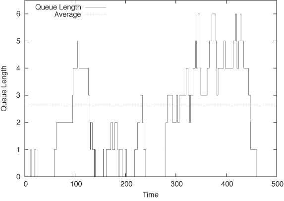
In a queueing problem, we are concerned only about arrivals and departures. A particularly important special case assumes that the rate at which customers arrive is constant over time and that arrivals at different times are independent of each other. (Notice that these are reasonable assumptions in many cases.) These two conditions imply that the number of arrivals during a certain time period t follows a Poisson distribution, since the Poisson distribution:
gives the probability of observing k Successes (arrivals, in our case) during an interval of length t if the “rate” of Successes is λ (see Chapter 9).
Another consequence is that the times between arrivals are distributed according to an exponential distribution:
p(t, λ) = λe–λt
The mean of the exponential distribution can be calculated without difficulty and equals 1/λ. It will often be useful to work with its inverse ta = 1/λ, the average interarrival time.
(It’s not hard to show that interarrival times are distributed
according to the exponential distribution when the number of
arrivals per time interval follows a Poisson distribution. Assume
that an arrival occurred at t = 0. Now we ask
for the probability that no arrival has
occurred by t = T; in
other words, p(0, T, λ) =
e–λT
because x0 = 1 and
0! = 1. Conversely, the probability that the next arrival will have
occurred sometime between t = 0 and
t = T is 1 –
p(0, T, λ). This is the
cumulative distribution function for the interarrival time, and from
it, we find the probability density for an arrival to occur at
t as 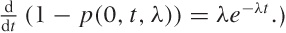
The appearance of the exponential distribution as the distribution of interarrival times deserves some comment. At first glance, it may seem surprising because this distribution is greatest for small interarrival times, seemingly favoring very short intervals. However, this observation has to be balanced against the infinity of possible interarrival times, all of which may occur! What is more important is that the exponential distribution is in a sense the most “random” way that interarrival times can be distributed: no matter how long we have waited since the last arrival, the probability that the next visitor will arrive after t more minutes is always the same: p(t, λ) = λe–λt. This property is often referred to as the lack of memory of the exponential distribution. Contrast this with a distribution of interarrival times that has a peak for some nonzero time: such a distribution describes a situation of scheduled arrivals, as we would expect to occur at a bus stop. In this scenario, the probability for an arrival to occur within the next t minutes will change with time.
Because the exponential distribution arises naturally from the
assumption of a constant arrival rate (and from the independence of
different arrivals), we have used it as the distribution of
interarrival times in the CustomerGenerator in the previous example.
It is less of a natural choice for the distribution of service times
(but it makes some theoretical arguments simpler).
The central question in all queueing problems concerns the expected length of the queue—not only how large it is but also whether it will settle down to a finite value at all, or whether it will “explode,” growing beyond all bounds.
In the simple memoryless, single-server–single-queue scenario that we have been investigating, the only two control parameters are the arrival rate λa and the service or exit rate λe; or rather their ratio:
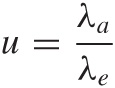
which is the fraction of time the server is busy. The quantity u is the server’s utilization. It is intuitively clear that if the arrival rate is greater than the exit rate (i.e., if customers are arriving at a faster rate then the server can process them), then the queue length will explode. However, it turns out that even if the arrival rate equals the service rate (so that u = 1), the queue length still grows beyond all bounds. Only if the arrival rate is strictly lower than the service rate will we end up with a finite queue.
Let’s see how this surprising result can be derived. Let pn be the probability of finding exactly n customers waiting in the queue. The rate at which the queue grows is λa, but the rate at which the queue grows from exactly n to exactly n + 1 is λa pn, since we must take into account the probability of the queue having exactly n members. Similarly, the probability of the queue shrinking from n + 1 to n members is λe pn+1.
In the steady state (which is the requirement for a finite queue length), these two rates must be equal:
λa pn = λe pn+1
which we can rewrite as:
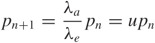
This relationship must hold for all n, and therefore we can repeat this argument and write pn = upn–1 and so on. This leads to an expression for pn in terms of p0:
pn = un p0
The probability p0 is the probability of finding no customer in the queue—in other words, it is the probability that the server is idle. Since the utilization is the probability for the server to be busy, the probability p0 for the server to be idle must be p0 = 1 – u.
We can now ask about the expected length L of the queue. We already know that the queue has length n with probability pn = un p0. Finding the expected queue length L requires that we sum over all possible queue lengths, each one weighted by the appropriate probability:
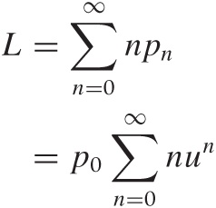
Now we employ a trick that is often useful for sums of this
form: observe that  and hence that
  . Using this expression in the sum for
L leads to:
. Using this expression in the sum for
L leads to:
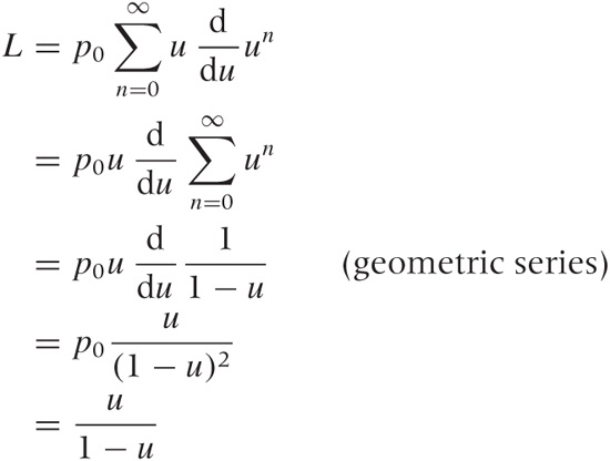
where we have used the sum of the geometric series (see Appendix B) and the expression for p0 = 1 – u. We can rewrite this expression directly in terms of the arrival and exit rates as:
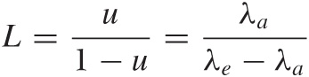
This is a central result. It gives us the expected length of the queue in terms of the utilization (or in terms of the arrival and exit rates). For low utilization (i.e., an arrival rate that is much lower than the service rate or, equivalently, an interarrival time that is much larger than the service time), the queue is very short on average. (In fact, whenever the server is idle, then the queue length equals 0, which drags down the average queue length.) But as the arrival rate approaches the service rate, the queue grows in length and becomes infinite when the arrival rate equals the service rate. (An intuitive argument for why the queue length will explode when the arrival rate equals the service time is that, in this case, the server never has the opportunity to “catch up.” If the queue becomes longer due to a chance fluctuation in arrivals, then this backlog will persist forever, since overall the server is only capable of keeping up with arrivals. The cumulative effect of such chance fluctuations will eventually make the queue length diverge.)
Running SimPy Simulations
In this section, we will try to confirm the previous result regarding the expected queue length by simulation. In the process, we will discuss a few practical points of using SimPy to understand queueing systems.
First of all, we must realize that each simulation run is only a particular realization of the sequence of events. To draw conclusions about the system in general, we therefore always need to perform several simulation runs and average their results.
In the previous listing, the simulation framework maintained
its state in the global environment. Hence, in order to rerun the
simulation, you had to restart the entire program! The program in
the next listing uses an alternative interface that encapsulates the
entire environment for each simulation run in an instance of class
Simulation. The global functions
initialize(), activate(), and simulate() are now member functions of
this Simulation object. Each
instance of the Simulation class
provides a separate, isolated simulation environment. A completely
new simulation run now requires only that we create a new instance
of this class.
The Simulation class is
provided by SimPy. Using it does not require any changes to the
previous program, except that the current instance of the Simulation class must be passed explicitly
to all simulation objects (i.e., instances of
Process and Resource and their subclasses):
from SimPy.Simulation import *
import random as rnd

interarrival_time = 10.0

class CustomerGenerator( Process ):
    def produce( self, bank ):
        while True:
            c = Customer( bank, sim=self.sim )
            c.start( c.doit() )
            yield hold, self, rnd.expovariate(1.0/interarrival_time)


class Customer( Process ):
    def __init__( self, resource, sim=None ):
        Process.__init__( self, sim=sim )
        self.bank = resource

    def doit( self ):
        yield request, self, self.bank
        yield hold, self, self.bank.servicetime()
        yield release, self, self.bank

class Bank( Resource ):
    def setServicetime( self, s ):
        self.service_time = s

    def servicetime( self ):
        return rnd.expovariate(1.0/self.service_time )


def run_simulation( t, steps, runs ):
    for r in range( runs ):

        sim = Simulation()
        sim.initialize()

        bank = Bank( monitored=True, monitorType=Tally, sim=sim )
        bank.setServicetime( t )

        src = CustomerGenerator( sim=sim )
        sim.activate( src, src.produce( bank ) )

        sim.startCollection( when=steps//2 )
        sim.simulate( until=steps )

        print t, bank.waitMon.mean()


t = 0
while t <= 11.0:
    t += 0.5
    run_simulation( t, 100000, 10 )
Another important change is that we don’t start recording
until half of the simulation time steps have passed (that’s what the
startCollection() method is for).
Remember that we are interested in the queue length in the
steady state—for that reason, we don’t want to
start recording until the system has settled down and any transient
behavior has disappeared.
To record the queue length, we now use a Tally object instead of a Monitor. The Tally will not allow us to replay the
entire sequence of events, but since we are only interested in the
average queue length, it is sufficient for our current
purposes.
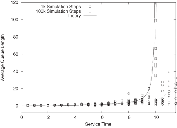
Finally, remember that as the utilization approaches u = 1 (i.e., as the service time approaches the interarrival time), we expect the queue length to become infinite. Of course, in any finite simulation it is impossible for the queue to grow to infinite length: the length of the queue is limited by the finite duration of the simulation run. The consequence of this observation is that, for utilizations near or above 1, the queue length that we will observe depends on the number of steps that we allow in the simulation. If we terminate the simulation too quickly, then the system will not have had time to truly reach its fully developed steady state and so our results will be misleading.
Figure 12-6 shows the results obtained when running the example program with 1,000 and 100,000 simulation steps. For low utilization (i.e., short queue lengths), the results from both data sets agree with each other (and with the theoretical prediction). However, as the service time approaches the interarrival time, the short simulation run does not last long enough for the steady state to form, and so the observed queue lengths are too short.
Summary
This concludes our tour of discrete event simulation with
SimPy. Of course, there is more to SimPy than mentioned here—in
particular, there are two additional forms of resources: the
Store and Level abstractions. Both of them not only
encapsulate a queue but also maintain an inventory (of individual
items for Store and of an
undifferentiated amount for Level). This inventory can be consumed or
replenished by simulation objects, allowing us to model inventory
systems of various forms. Other SimPy facilities to explore include
asynchronous events, which can be received by simulation objects as
they are waiting in queue and additional recording and tracing
functionality. The project documentation will provide further
details.
Further Reading
A First Course in Monte Carlo. George S. Fishman. Duxbury Press. 2005.
This book is a nice introduction to Monte Carlo simulations and includes many topics that we did not cover. Requires familiarity with calculus.
Bootstrap Methods and Their Application. A. C. Davison and D. V. Hinkley. Cambridge University Press. 1997.
The bootstrap is actually a fairly simple and practical concept, but most books on it are very theoretical and difficult, including this one. But it is comprehensive and relatively recent.
Applied Probability Models. Do Le Paul Minh. Duxbury Press. 2000.
The theory of random processes is difficult, and the results often don’t seem commensurate with the amount of effort required to obtain them. This book (although possibly hard to find) is one of the more accessible ones.
Introduction to Stochastic Processes. Gregory F. Lawler. Chapman & Hall/CRC. 2006.
This short book is much more advanced and theoretical than the previous one. The treatment is concise and to the point.
Introduction to Operations Research. Frederick S. Hillier and Gerald J. Lieberman. 9th ed., McGraw-Hill. 2009.
The field of operations research encompasses a set of mathematical methods that are relevant for many problems arising in a business or industrial setting, including queueing theory. This text is a standard introduction.
Fundamentals of Queueing Theory. Donald Gross, John F. Shortle, James M. Thompson, and Carl M. Harris. 4th ed., Wiley. 2008.
The standard textbook on queueing theory. Not for the faint of heart.