Table of Contents for

Data Analysis with Open Source Tools

The data set is a classic: the CO₂ measurements above Mauna Loa on Hawaii. The inspiration for this section comes from Cleveland’s Elements of Graphical Analysis,^[12] but the approach is entirely mine.

First question: what’s in the data set? I see that the first column represents the date (month and year) while the second contains the measured CO₂ concentration in parts per million. Here are the first few lines:

Jan-1959      315.42
Feb-1959      316.32
Mar-1959      316.49
Apr-1959      317.56
...

The measurements are regularly spaced (in fact, monthly), so I don’t need to parse the date in the first column; I simply plot the second column by itself. (In the figure, I have added tick labels on the horizontal axis for clarity, but I am omitting the commands required here—they are not essential.)

Figure 6-1. The first look at the data: plot “data”u1wl

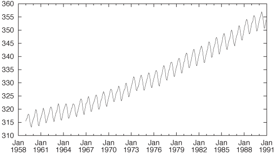
plot "data" u 2 w l

The plot shows a rather regular short-term variation overlaid on a nonlinear upward trend. (See Figure 6-1.)

The coordinate system is not convenient for mathematical modeling: the x axis is not numeric, and for modeling purposes it is usually helpful if the graph goes through the origin. So, let’s make it do so by subtracting the vertical offset from the data and expressing the horizontal position as the number of months since the first measurement. (This corresponds to the line number in the data file, which is accessible in a gnuplot session through the pseudo-column with column number 0.)

plot "data" u 0:($2-315) w l

A brief note on the command: the specification after the u (short for using) gives the columns to be used for the x and y coordinates, separated by a colon. Here we use the line number (which is in the pseudo-column 0) for the x coordinate. Also, we subtract the constant offset 315 from the values in the second column and use the result as the y value. Finally, we plot the result with lines (abbreviated w l) instead of using points or other symbols. See Figure 6-2.

The most predominant feature is the trend. What can we say about it? First of all, the trend is nonlinear: if we ignore the short-term variation, the curve is convex downward. This suggests a power law with an as-yet-unknown exponent: x^k. All power-law functions go through the origin (0, 0) and also through the point (1, 1). We already made sure that the data passes through the origin, but to fix the upper-right corner, we need to rescale both axes: if x^k goes through (1, 1), then goes through (a, b).

Figure 6-2. Making the x values numeric and subtracting the constant vertical offset: plot “data” u 0:($2-315) w l

Figure 6-3. Adding a function: plot “data” u 0:($2-315) w l, 35*(x/350)**2

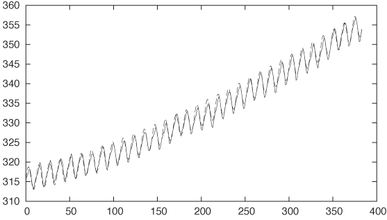
What’s the value for the exponent k? All I know about it right now is that it must be greater than 1 (because the function is convex). Let’s try k = 2. (See Figure 6-3.)

plot "data" u 0:($2-315) w l, 35*(x/350)**2

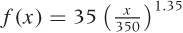
Not bad at all! The exponent is a bit too large—some fiddling suggests that k = 1.35 would be a good value (see Figure 6-4).

plot "data" u 0:($2-315) w l, 35*(x/350)**1.35

To verify this, let’s plot the residual; that is, we subtract the trend from the data and plot what’s left. If our guess for the trend is correct, then the residual should not exhibit any trend itself—it should just straddle y = 0 in a balanced fashion (see Figure 6-5).

plot "data" u 0:($2-315 - 35*($0/350)**1.35) w l

Figure 6-4. Getting the exponent right:

Figure 6-5. The residual, after subtracting the function from the data.

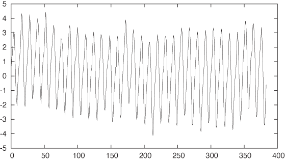
It might be hard to see the longer-term trend in this data, so we may want to approximate it by a smoother curve. We can use the weighted-spline approximation built into gnuplot for that purpose. It takes a third parameter, which is a measure for the smoothness: the smaller the third parameter, the smoother the resulting curve; the larger the third parameter, the more closely the spline follows the original data (see Figure 6-6).

plot "data" u 0:(2 − 315 − 35 * (0/350)**1.35) w l, \
     "" u 0:($2-315 - 35*($0/350)**1.35):(0.001) s acs w l

At this point, the expression for the function that we use to approximate the data has become unwieldy. Thus it now makes sense to define it as a separate function:

f(x) = 315 + 35*(x/350)**1.35
plot "data" u 0:($2-f($0)) w l, "" u 0:($2-f($0)):(0.001) s acs w l

Figure 6-6. Plotting a smoothed version of the residual together with the unsmoothed residual to test whether there is any systematic trend remaining in the residual.

From the smoothed line we can see that the overall residual is pretty much flat and straddles zero. Apparently, we have captured the overall trend quite well: there is little evidence of a systematic drift remaining in the residuals.

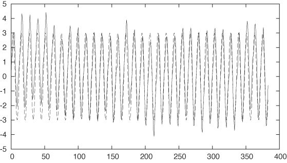
With the trend taken care of, the next feature to tackle is the seasonality. The seasonality seems to consist of rather regular oscillations, so we should try some combination of sines and cosines. The data pretty much starts out at y = 0 for x = 0, so we can try a sine by itself. To make a guess for its wavelength, we recall that the data is meteorological and has been taken on a monthly basis—perhaps there is a year-over-year periodicity. This would imply that the data is the same every 12 data points. If so, then a full period of the sine, which corresponds to 2π, should equal a horizontal distance of 12 points. For the amplitude, the graph suggests a value close to 3 (see Figure 6-7).

plot "data" u 0:($2-f($0)) w l, 3*sin(2*pi*x/12) w l

Right on! In particular, our guess for the wavelength worked out really well. This makes sense, given the origin of the data.

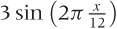
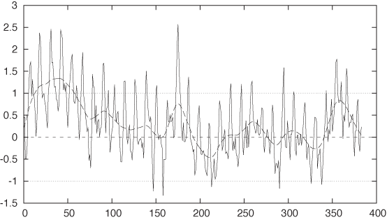
Let’s take residuals again, employing splines to see the bigger picture as well (see Figure 6-8):

f(x) = 315 + 35*(x/350)**1.35 + 3*sin(2*pi*x/12)
plot "data" u 0:($2-f($0)) w l, "" u 0:($2-f($0)):(0.001) s acs w l

The result is pretty good but not good enough. There is clearly some regularity remaining in the data, although at a higher frequency than the main seasonality. Let’s zoom in on a smaller interval of the data to take a closer look. The data in the interval [60:120] appears particularly regular, so let’s look there (see Figure 6-9):

plot [60:120] "data" u 0:($2-f($0)) w lp, "" u 0:($2-f($0)):(0.001) s acs w l

Figure 6-7. Fitting the seasonality with a sine wave:

Figure 6-8. Residuals after subtracting both trend and seasonality.

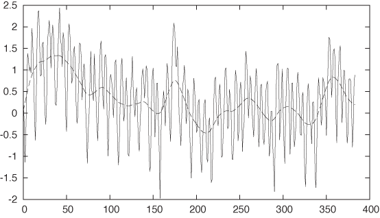
I have indicated the individual data points using gnuplot’s linespoints (lp) style. We can now count the number of data points between the main valleys in the data: 12 points. This is the main seasonality. But it seems that between any two primary valleys there is exactly one secondary valley. Of course: higher harmonics! The original seasonality had a period of exactly 12 months, but its shape was not entirely symmetric: its rising flank comprised 7 months but the falling flank only 5 (as you can see by zooming in on the original data with only the trend removed). This kind of asymmetry implies that the seasonality cannot be represented by a simple sine wave alone but that we have to take into account higher harmonics—that is, sine functions with frequencies that are integer multiples of the primary seasonality. So let’s try the first higher harmonic, again punting a little on the amplitude (see Figure 6-10):

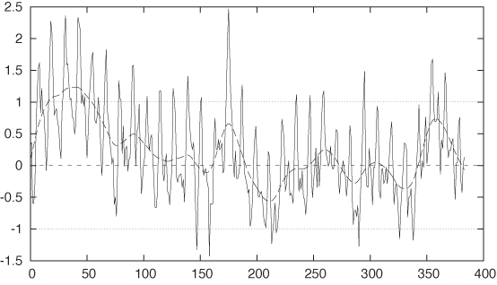
f(x) = 315 + 35*(x/350)**1.35 + 3*sin(2*pi*x/12) - 0.75*sin(2*pi*$0/6)
plot "data" u 0:($2-f($0)) w l, "" u 0:($2-f($0)):(0.001) s acs w l

Figure 6-9. Zooming in for a closer look. Individual data points are marked by symbols.

Figure 6-10. Residual after removing trend and the first and second harmonic of the seasonality.

Now we are really pretty close. Look at the residual—in particular, for values of x greater than about 150. The data starts to look quite “random,” although there is some systematic behavior for x in the range [0:70] that we don’t really capture. Let’s add some constant ranges to the plot for comparison (see Figure 6-11):

plot "data" u 0:($2-f($0)) w l, "" u 0:($2-f($0)):(0.001) s acs w l, 0, 1, -1

It looks as if the residual is skewed toward positive values, so let’s adjust the vertical offset by 0.1 (see Figure 6-12):

f(x) = 315 + 35*(x/350)**1.35 + 3*sin(2*pi*x/12) - 0.75*sin(2*pi*$0/6) + 0.1
plot "data" u 0:($2-f($0)) w l, "" u 0:($2-f($0)):(0.001) s acs w l, 0, 1, -1

Figure 6-11. Adding some grid lines for comparison.

Figure 6-12. The final residual.

That’s now really close. You should notice how small the last adjustment was—we started out with data ranging from 300 to 350, and now we are making adjustments to the parameters on the order of 0.1. Also note how small the residual has become: mostly in the range from –0.7 to 0.7. That’s only about 3 percent of the total variation in the data.

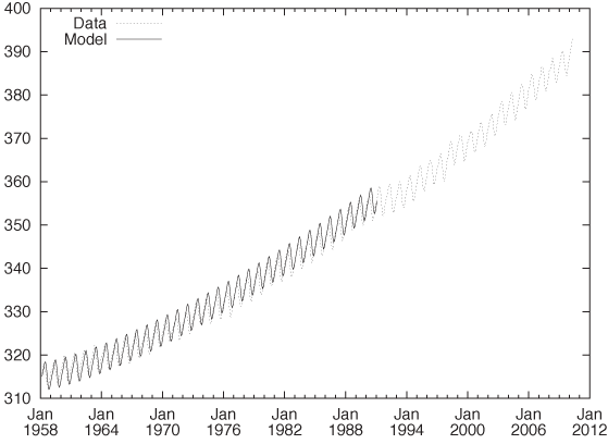
Finally, let’s look at the original data again, this time together with our analytical model (see Figure 6-13):

f(x) = 315 + 35*(x/350)**1.35 + 3*sin(2*pi*x/12) - 0.75*sin(2*pi*$0/6) + 0.1
plot "data" u 0:2 w l, f(x)

All in all, pretty good.

Figure 6-13. The raw data with the final fit.

So what is the point here? The point is that we started out with nothing—no idea at all of what the data looked like. And then, layer by layer, we peeled off components of the data, until only random noise remained. We ended up with an explicit, analytical formula that describes the data remarkably well.

But there is something more. We did so entirely “manually”: by plotting the data, trying out some approximations, and wiggling the numbers until they agreed reasonably well with the data. At no point did we resort to a black-box fitting routine—because we didn’t have to! We did just fine. (In fact, after everything was finished, I tried to perform a nonlinear fit using the functional form of the analytical model as we have worked it out—only to have it explode terribly! The model depends on seven parameters, which means that convergence of a nonlinear fit can be a bit precarious. In fact, it took me longer to try to make the fit work than it took me to work the parameters out manually as just demonstrated.)

I’d go even further. We learned more by doing this work manually than if we had used a fitting routine. Some of the observations (such as the idea to include higher harmonics) arose only through direct interaction with the data. And it’s not even true that the parameters would be more accurate if they had been calculated by a fitting routine. Sure, they would contain 16 digits but not more information. Our manual wiggling of the parameters enabled us to see quickly and directly the point at which changes to the parameters are so small that they no longer influence the agreement between the data and the model. That’s when we have extracted all the information from the data—any further “precision” in the parameters is just insignificant noise.

You might want to try your hand at this yourself and also experiment with some variations of your own. For example, you may question the choice of the power-law behavior for the long-term trend. Does an exponential function (like exp(x)) give a better fit? It is not easy to tell from the data, but it makes a huge difference if we want to project our findings significantly (10 years or more) into the future. You might also take a closer look at the seasonality. Because it is so regular—and especially since its period is known exactly—you should be able to isolate just the periodic part of the data in a separate model by averaging corresponding months for all years. Finally, there is 20 years’ worth of additional data available beyond the “classic” data set used in my original exploration.^[13] Figure 6-14 shows all the available data together with the model that we have developed. Does the fit continue to work well for the years past 1990?

Figure 6-14. The extended data set up to early 2010 together with the model (up to 1990).

The example commands in this chapter should have given you a good idea what working with gnuplot is like, but let’s take a quick look at some of the basics.

Gnuplot (http://www.gnuplot.info) is command-line oriented: when you start gnuplot, it presents you with a text prompt at which to enter commands; the resulting graphs are shown in a separate window. Creating plots is simple—the command:

plot sin(x) with lines, cos(x) with linespoints

will generate a plot of (you guessed it) a sine and a cosine. The sine will be drawn with plain lines, and the cosine will be drawn with symbols (“points”) connected by lines. (Many gnuplot keywords can be abbreviated: instead of with lines I usually type: w l, or w lp instead of with linespoints. These short forms are a major convenience although rather cryptic in the beginning. In this short introductory section, I will make sure to only use the full forms of all commands.)

To plot data from a file, you also use the plot command; for instance:

plot "data" using 1:2 with lines

When plotting data from a file, we use the using keyword to specify which columns from the file we want to plot—in the command just given, we use entries from the first column as x values and use entries from the second column for y values.

One of the nice features of gnuplot is that you can apply arbitrary transformations to the data as it is being plotted. To do so, you put parentheses around each entry in the column specification that you want to apply a transform to. Within these parentheses you can use any mathematical expression. The data from each column is available by prefixing the column index by the dollar sign. An example will make this more clear:

plot "data" using (1/$1):($2+$3) with lines

This command plots the sum of the second and third columns (that is: $2+$3) as a function of one over the value in the first column (1/$1).

It is also possible to mix data and functions in a single plot command (as we have seen in the examples in this chapter):

plot "data" using 1:2 with lines, cos(x) with lines

This is different from the Matlab-style of plotting, where a function must be explicitly evaluated for a set of points before the resulting set of values can be plotted.

We can now proceed to add decorations (such as labels and arrows) to the plot. All kinds of options are available to customize virtually every aspect of the plot’s appearance: tick marks, the legend, aspect ratio—you name it. When we are done with a plot, we can save all the commands used to create it (including all decorations) via the save command:

save "plot.gp"

Now we can use load "plot.gp" to re-create the graph.

As you can see, gnuplot is extremely straightforward to use. The one area that is often regarded as somewhat clumsy is the creation of graphs in common graphics file formats. The reason for this is historical: the first version of gnuplot was written in 1985, a time when one could not expect every computer to be connected to a graphics-capable terminal and when many of our current file formats did not even exist! The gnuplot designers dealt with this situation by creating the so-called “terminal” abstraction. All hardware-specific capabilities were encapsulated by this abstraction so that the rest of gnuplot could be as portable as possible. Over time, this “terminal” came to include different graphics file formats as well (not just graphics hardware terminals), and this usage continues to this day. Exporting a graph to a common file format (such as GIF, PNG, PostScript, or PDF) requires a five-step process:

set terminal png
set output "plot.png"
replot
set terminal wxt
set output

In the first step, we choose the output device or “terminal”: here, a PNG file. In the second step, we choose the file name. In the third step, we explicitly request that the graph be regenerated for this newly chosen device. The remaining commands restore the interactive session by selecting the interactive wxt terminal (built on top of the wxWidgets widget set) and redirecting output back to the interactive terminal. If you find this process clumsy and error-prone, then you are not alone, but rest assured: gnuplot allows you to write macros, which can reduce these five steps to one!

I should mention one further aspect of gnuplot: because it has been around for 25 years, it is extremely mature and robust when it comes to dealing with typical day-to-day problems. For example, gnuplot is refreshingly unpicky when it comes to parsing input files. Many other data analysis or plotting programs that I have seen are pretty rigid in this regard and will bail when encountering unexpected data in an input file. This is the right thing to do in theory, but in practice, data files are often not clean—with ad hoc formats and missing or corrupted data points. Having your plotting program balk over whitespace instead of tabs is a major nuisance when doing real work. In contrast, gnuplot usually does an amazingly good job at making sense of almost any input file you might throw at it, and that is indeed a great help. Similarly, gnuplot recognizes undefined mathematical expressions (such as 1/0, log(0), and so on) and discards them. This is also very helpful, because it means that you don’t have to worry about the domains over which functions are properly defined while you are in the thick of things. Because the output is graphical, there is usually very little risk that this silent discarding of undefined values will lead you to miss essential behavior. (Things are different in a computer program, where silently ignoring error conditions usually only compounds the problem.)