Table of Contents for
Data Analysis with Open Source Tools
 Data Analysis with Open Source Tools
Published by
O'Reilly Media, Inc., 2010
Data Analysis with Open Source Tools
Published by
O'Reilly Media, Inc., 2010
- Cover
- Data Analysis with Open Source Tools
- O'Reilly Strata Conference
- Data Analysis with Open Source Tools
- Dedication
- A Note Regarding Supplemental Files
- Preface
- 1. Introduction
- I. Graphics: Looking at Data
- 2. A Single Variable: Shape and Distribution
- 3. Two Variables: Establishing Relationships
- 4. Time As a Variable: Time-Series Analysis
- 5. More Than Two Variables: Graphical Multivariate Analysis
- 6. Intermezzo: A Data Analysis Session
- II. Analytics: Modeling Data
- 7. Guesstimation and the Back of the Envelope
- 8. Models from Scaling Arguments
- 9. Arguments from Probability Models
- 10. What You Really Need to Know About Classical Statistics
- 11. Intermezzo: Mythbusting—Bigfoot, Least Squares, and All That
- III. Computation: Mining Data
- 12. Simulations
- 13. Finding Clusters
- 14. Seeing the Forest for the Trees: Finding Important Attributes
- 15. Intermezzo: When More Is Different
- IV. Applications: Using Data
- 16. Reporting, Business Intelligence, and Dashboards
- 17. Financial Calculations and Modeling
- 18. Predictive Analytics
- 19. Epilogue: Facts Are Not Reality
- A. Programming Environments for Scientific Computation and Data Analysis
- B. Results from Calculus
- C. Working with Data
- D. About the Author
- Index
- About the Author
- Colophon
- Copyright
Chapter 13. Finding Clusters
THE TERM CLUSTERING REFERS TO THE PROCESS OF FINDING GROUPS OF POINTS WITHIN A DATA SET THAT ARE IN some way “lumped together.” It is also called unsupervised learning—unsupervised because we don’t know ahead of time where the clusters are located or what they look like. (This is in contrast to supervised learning or classification, where we attempt to assign data points to preexisting classes; see Chapter 18.)
I regard clustering as an exploratory method: a computer-assisted (or even computationally driven) approach to discovering structure in a data set. As an exploratory technique, it usually needs to be followed by a confirmatory analysis that validates the findings and makes them more precise.
Clustering is a lot of fun. It is a rich topic with a wide variety of different problems, as we will see in the next section, where we discuss the different kinds of cluster one may encounter. The topic also has a lot of intuitive appeal, and most clustering methods are rather straightforward. This allows for all sorts of ad hoc modifications and enhancements to accommodate the specific problem one is working on.
What Constitutes a Cluster?
Clustering is not a very rigorous field: there are precious few established results, rigorous theorems, or algorithmic guarantees. In fact, the whole notion of a “cluster” is not particularly well defined. Descriptions such as “groups of points that are similar” or “close to each other” are insufficient, because clusters must also be well separated from each other. Look at Figure 13-1: some points are certainly closer to each other than to other points, yet there are no discernible clusters. (In fact, it is an interesting exercise to define what constitutes the absence of clusters.) This leads to one possible definition of clusters: contiguous regions of high data point density separated by regions of lower point density. Although not particularly rigorous either, this description does seem to capture the essential elements of typical clusters. (For a different point of view, see the next section.)
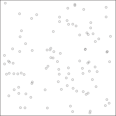
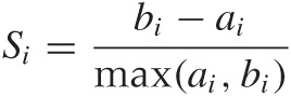
The definition just proposed allows for very different kinds of clusters. Figure 13-2 and Figure 13-3 show two very different types. Of course, Figure 13-2 is the “happy” case, showing a data set consisting of well-defined and clearly separated regions of high data point density. The clusters in Figure 13-3 are of a different type, one that is more easily thought of by means of nearest-neighbor (graph) relationships than by point density. Yet in this case as well, there are higher density regions separated by lower density regions—although we might want to exploit the nearest-neighbor relationship instead of the higher density when developing with a practical algorithm for this case.
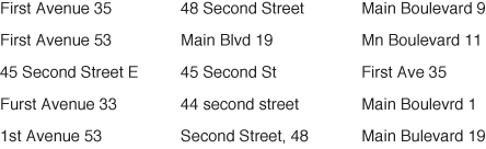
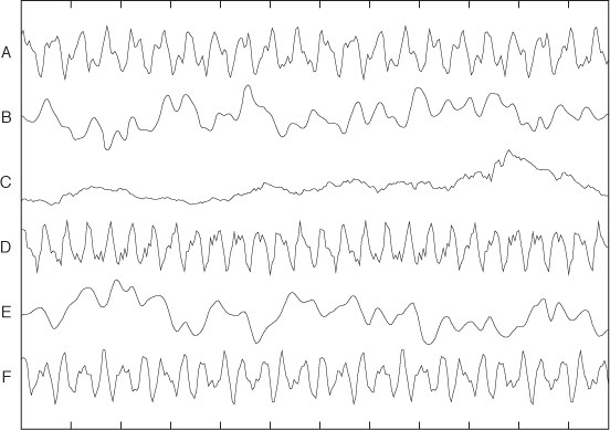
Clustering is not limited to points in space. Figure 13-4 and Figure 13-5 show two rather different cases for which it nevertheless makes sense to speak of clusters. Figure 13-4 shows a bunch of street addresses. No two of them are exactly the same, but if we look closely, we will easily recognize that all of them can be grouped into just a few neighborhoods. Figure 13-5 shows a bunch of different time series: again, some of them are more alike than others. The challenge in both of these examples is finding a way to express the “similarity” among these nonnumeric, nongeometric objects!
Finally, we should keep in mind that clusters may have complicated shapes. Figure 13-6 shows two very well-behaved clusters as distinct regions of high point density. However, complicated and intertwined shapes of the regions will challenge many commonly used clustering algorithms.
A bit of terminology can help to distinguish different cluster shapes. If the line connecting any two points lies entirely within the cluster itself (as in Figure 13-2), then the cluster is convex. This is the easiest shape to handle. A cluster is convex only if the connecting line between two points lies entirely within the cluster for all pairs of points. Sometimes this is not the case, but we can still find at least one point (the center) such that the connecting line from the center to any other point lies entirely within the cluster: such a cluster is called star convex. Notice that the clusters in Figure 13-6 are neither convex nor star convex. Sometimes one cluster is entirely surrounded by another cluster without actually being part of it: in this case we speak of a nested cluster. Nested clusters can be particularly challenging (see Figure 13-3).
A Different Point of View
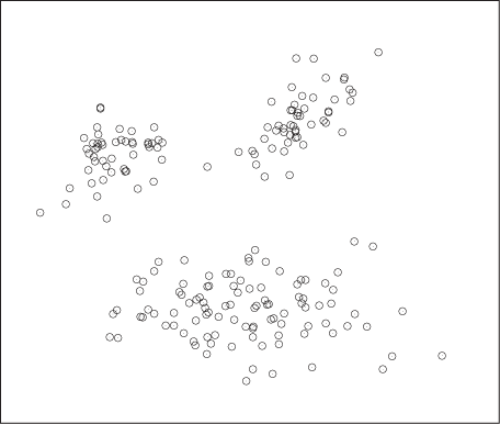
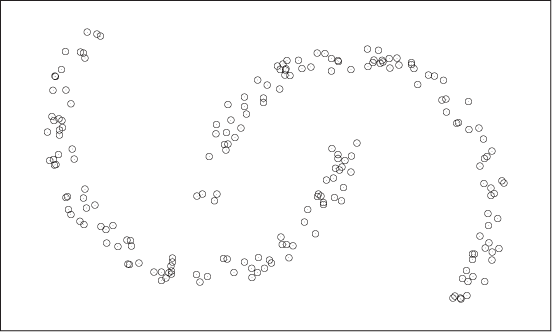
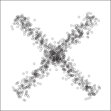
In the absence of a precise (mathematical) definition, a cluster can be whatever we consider as one. That is important because our minds have a different, alternative way of grouping (“clustering”) objects: not by proximity or density but rather by the way objects fit into a larger structure. Figure 13-7 and Figure 13-8 show two examples.
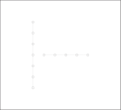
Intuitively, we have no problem grouping the points in Figure 13-7 into two overlapping clusters. Yet, the density-based definition of a cluster we proposed earlier will not support such a conclusion. Similar considerations apply to the set of points in Figure 13-8. The distance between any two adjacent points is the same, but we perceive the larger structures of the vertical and horizontal arrangements and assign points to clusters based on them.
This notion of a cluster does not hinge on the similarity or proximity of any pair of points to each other but instead on the similarity between a point and a property of the entire cluster. For any algorithm that considers a single point (or a single pair of points) at a time, this leads to a problem: to determine cluster membership, we need the property of the whole cluster; but to determine the properties of the cluster, we must first assign points to clusters.
To handle such situations, we would need to perform some kind of global structure analysis—a task our minds are incredibly good at (which is why we tend to think of clusters this way) but that we have a hard time teaching computers to do. For problems in two dimensions, digital image processing has developed methods to recognize and extract certain features (such as edge detection). But general clustering methods, such as those described in the rest of this chapter, deal only with local properties and therefore can’t handle problems such as those in Figure 13-7 and Figure 13-8.
Distance and Similarity Measures
Given how strongly our intuition about clustering is shaped by geometric problems such as those in Figure 13-2 and Figure 13-3, it is an interesting and perhaps surprising observation that clustering does not actually require data points to be embedded into a geometric space: all that is required is a distance or (equivalently) a similarity measure for any pair of points. This makes it possible to perform clustering on a set of strings, such as those in Figure 13-4 that do not map to points in space. However, if the data points have properties of a vector space (see Appendix C), then we can develop more efficient algorithms that exploit these properties.
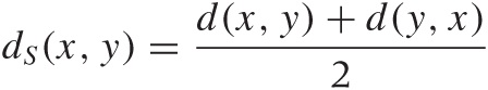
A distance is any function d(x, y) that takes two points and returns a scalar value that is a measure for how different these points are: the more different, the larger the distance. Depending on the problem domain, it may make more sense to express the same information in terms of a similarity function s(x, y), which returns a scalar that tells us how similar two points are: the more different they are, the smaller the similarity. Any distance can be transformed into a similarity and vice versa. For example if we know that our similarity measure s can take on values only in the range [0, 1], then we can form an equivalent distance by setting d = 1 – s. In other situations, we might decide to use d = 1/s, or s = e–d, and so on; the choice will depend on the problem we are working on. In what follows, I will express problems in terms of either distances or similarities, whichever seems more natural. Just keep in mind that you can always transform between the two.
How we define a distance function is largely up to us, and we can express different semantics about the data set through the appropriate choice of distance. For some problems, a particular distance measure will present itself naturally (if the data points are points in space, then we will most likely employ the Euclidean distance or a measure similar to it), but for other problems, we have more freedom to define our own metric. We will see several examples shortly.
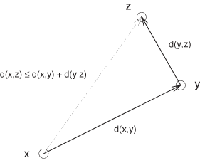
There are certain properties that a distance (or similarity) function should have. Mathematicians have developed a set of properties that a function must possess to be considered a metric (or distance) in a mathematical sense. These properties can provide valuable guidance, but don’t take them too seriously: for our purposes, different properties might be more important. The four axioms of a mathematical metric are:
d(x, y) | ≥ 0 | |
d(x, y) | = 0 | if and only if x = y |
d(x, y) | = d(y, x) | |
d(x, y) + d(y, z) | ≥ d(x, z) | |
The first two axioms state that a distance is always positive and that it is null only if the two points are equal. The third property (“symmetry”) states that the distance between x and y is the same as the distance between y and x—no matter which way we consider the pair. The final property is the so-called triangle inequality, which states that to get from x to z, it is never shorter to take a detour through a third point y instead of going directly (see Figure 13-9).
This all seems rather uncontroversial, but these conditions are not necessarily fulfilled in practice. A funny example for an asymmetric distance occurs if you ask everyone in a group of people how much they like every other member of the group and then use the responses to construct a distance measure: it is not at all guaranteed that the feelings of person A for person B are requited by B. (Using the same example, it is also possible to construct scenarios that violate the triangle inequality.) For technical reasons, the symmetry property is usually highly desirable. You can always construct a symmetric distance function from an asymmetric one:
is always symmetric.
One property of great practical importance but not included among the distance axioms is smoothness. For example, we could define a rather simple-minded distance function that is 0 if and only if both points are equal to each other and that is 1 if the two points are not equal:
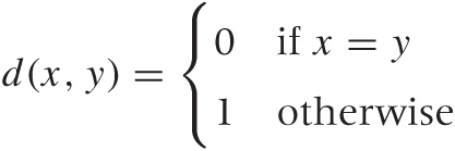
You can convince yourself that this distance fulfills all four of the distance axioms. However, this is not a very informative distance measure, because it gives us no information about how different two nonidentical points are! Most clustering algorithms require this information. A certain kind of tree-based algorithm, for example, works by successively considering the pairs of points with the smallest distance between them. When using this binary distance, the algorithm will make only limited progress before having exhausted all information available to it.
The practical upshot of this discussion is that a good distance function for clustering should change smoothly as its inputs become more or less similar. (For classification tasks, a binary one as in the example just discussed might be fine.)
Common Distance and Similarity Measures
Depending on the data set and the purpose of our analysis, there are different distance and similarity measures available.
First, let’s clarify some terminology. We are looking for ways
to measure the distance between any two data points. Very often, we
will find that a point has a number of
dimensions or features.
(The first usage is more common for numerical data, the latter for
categorical data.) In other words, each point is a collection of
individual values: x =
{x1,
x2,...,
xd},
where d is the number of dimensions (or
features). For example, the data point {0, 1} has two dimensions and
describes a point in space; whereas the tuple [ 'male', 'retired', 'Florida' ], which
describes a person, has three features.
For any given data set containing n elements, we can form n2 pairs of points. The set of all distances for all possible pairs of points can be arranged in a quadratic table known as the distance matrix. The distance matrix embodies all information about the mutual relationships between all points in the data set. If the distance function is symmetric, as is usually the case, then the matrix is also symmetric. Furthermore, the entries along the main diagonal typically are all 0, since d(x, x) = 0 for most well-behaved distance functions.
Numerical data
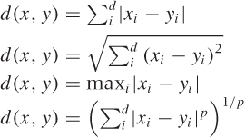
If the data is numerical and also “mixable” or vector-like (in the sense of Appendix C), then the data points bear a strong resemblance to points in space; hence we can use a metric such as the familiar Euclidean distance. The Euclidean distance is the most commonly used from a large family of related distance measures, which also contains the so-called Manhattan (or taxicab) distance and the maximum (or supremum) distance. All of these are in fact special cases of a more general Minkowski or p-distance.[21] Table 13-1 shows some examples. (The Manhattan distance is so named because it measures distances the way a New York taxicab moves: at right angles, along the city blocks. The Euclidean distance measures distances “as the crow flies.” Finally, it is an amusing exercise to show that the maximum distance corresponds to the Minkowski p-distance as p → ∞.)
All these distance measures have very similar properties, and the differences between them usually do not matter much. The Euclidean distance is by far the most commonly used. I list the others here mostly to give you a sense of the kind of leeway that exists in defining a suitable distance measure—without significantly affecting the results!
If the data is numeric but not mixable (so that it does not make sense to add a random fraction of one data set to a random fraction of a different data set), then these distance measures are not appropriate. Instead, you may want to consider a metric based on the correlation between two data points.
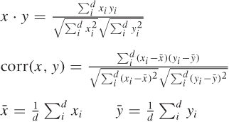
Correlation-based measures are measures of similarity: they are large when objects are similar and small when the objects are dissimilar. There are two related measures: the dot product and the correlation coefficient, which are also defined in Table 13-1. The only difference is that when calculating the correlation coefficient, we first center both data points by subtracting their respective means.
In both measures, we multiply entries for the same “dimension” and sum the results; then we divide by the correlation of each data point with itself. Doing so provides a normalization and ensures that the correlation of any point with itself is always 1. This normalization step makes correlation-based distance measures suitable for data sets containing data points with widely different numeric values.
By construction, the value of a dot product always falls in the interval [0, 1], and the correlation coefficient always falls in the interval [–1, 1]. You can therefore transform either one into a distance measure if need be (e.g., if d is the dot product, then 1 – d is a proper distance).
I should point out that the dot product has a geometric meaning. If we regard the data points as vectors in some suitable space, then the dot product of two points is the cosine of the angle that the two vectors make with each other. If they are perfectly aligned (i.e., they fall onto each other), then the angle is 0 and the cosine (and the correlation) is 1. If they are at right angles to each other, the cosine is 0.
Correlation-based distance measures are suitable whenever numeric data is not readily mixable—for instance, when evaluating the similarity of the time series in Figure 13-5.
Categorical data
If the data is categorical, then we can count the number of features that do not agree in both data points (i.e., the number of mismatched features); this is the Hamming distance. (We might want to divide by the total number of features to obtain a number between 0 and 1, which is the fraction of mismatched features.)
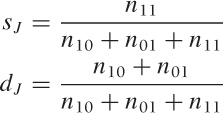
In certain data mining problems, the number of features is large, but only relatively few of them will be present for each data point. Moreover, the features may be binary: we care only whether or not they are present, but their values don’t matter. (As an example, imagine a patient’s health record: each possible medical condition constitutes a feature, and we want to know whether the patient has ever suffered from it.) In such situations, where features are not merely categorical but binary and sparse (meaning that just a few of the features are On), we may be more interested in matches between features that are On than in matches between features that are Off. This leads us to the Jaccard coefficient sJ, which is the number of matches between features that are On for both points, divided by the number of features that are On in at least one of the data points. The Jaccard coefficient is a similarity measure; the corresponding distance function is the Jaccard distance dJ = 1 – sJ .
n00 | features that are Off in both points |
n10 | features that are On in the first point, and Off in the second point |
n01 | features that are Off in the first point, and On in the second point |
n11 | features that are On in both points |
There are many other measures of similarity or dissimilarity for categorical data, but the principles are always the same. You calculate some fraction of matches, possibly emphasizing one aspect (e.g., the presence or absence of certain values) more than others. Feel free to invent your own—as far as I can see, none of these measures has achieved universal acceptance or is fundamentally better than any other.
String data
If the data consists of strings, then we can use a form of Hamming distance and count the number of mismatches. If the strings in the data set are not all of equal length, we can pad the shorter string and count the number of characters added as mismatches.
If we are dealing with many strings that are rather similar to each other (distorted through typos, for instance), then we can use a more detailed measure of the difference between them—namely the edit or Levenshtein distance. The Levenshtein distance is the minimum number of single-character operations (insertions, deletions, and substitutions) required to transform one string into the other. (A quick Internet search will give many references to the actual algorithm and available implementations.)
Another approach is to find the length of the longest common subsequence. This metric is often used for gene sequence analysis in computational biology.
This may be a good place to make a more general point: the best distance measure to use does not follow automatically from data type; rather, it depends on the semantics of the data—or, more precisely, on the semantics that you care about for your current analysis! In some cases, a simple metric that only calculates the difference in string length may be perfectly sufficient. In another case, you might want to use the Hamming distance. If you really care about the details of otherwise similar strings, the Levenshtein distance is most appropriate. You might even want to calculate how often each letter appears in a string and then base your comparison on that. It all depends on what the data means and on what aspect of it you are interested at the moment (which may also change as the analysis progresses). Similar considerations apply everywhere—there are no “cookbook” rules.
Special-purpose metrics
A more abstract measure for the similarity of two points is based on the number of neighbors that the two points have in common; this metric is known as the shared nearest neighbor (SNN) similarity. To calculate the SNN for two points x and y, you find the k nearest neighbors (using any suitable distance function) for both x and y. The number of neighbors shared by both points is their mutual SNN.
The same concept can be extended to cases in which there is some property that the two points may have in common. For example, in a social network we could define the “closeness” of two people by the number of friends they share, by the number of movies they have both seen, and so on. (This application is equivalent to the Hamming distance.) Nearest-neighbor-based metrics are particularly suitable for high-dimensional data, where other distance measures can give spuriously small results.
Finally, let me remind you that sometimes the solution does not consist of inventing a new metric. Instead, the trick is to map the problem to a different space that already has a predefined, suitable metric.
As an example, consider the problem of measuring the degree of similarity between different text documents (we here assume that these documents are long—hundreds or thousands of words). The standard approach to this problem is to count how often each word appears in each document. The resulting data structure is referred to as the document vector. You can now form a dot product between two document vectors as a measure of their correspondence.
Technically speaking, we have mapped each document to a point in a (high-dimensional) vector space. Each distinct word that occurs in any of the documents spans a new dimension, and the frequency with which each word appears in a document provides the position of that document along this axis. This is very interesting, because we have transformed highly structured data (text) into numerical, even vector-like data and can therefore now manipulate it much more easily. (Of course, the benefit comes at a price: in doing so we have lost all information about the sequence in which words appeared in the text. It is a separate consideration whether this is relevant for our purpose.)
One last comment: one can overdo it when defining distance and similarity measures. Complicated or sophisticated definitions are usually not necessary as long as you capture the fundamental semantics. The Hamming distance and the document vector correlation are two good examples of simplified metrics that intentionally discard a lot of information yet still turn out to be highly successful in practice.
Clustering Methods
In this section, we will discuss several very different clustering algorithms. As you will see, the basic ideas behind all three algorithms are rather simple, and it is straightforward to come up with perfectly adequate implementations of them yourself. These algorithms are also important as starting points for more sophisticated clustering routines, which usually augment them with various heuristics or combine ideas from different algorithms.
Different algorithms are suitable for different kinds of problems—depending, for example, on the shape and structure of the clusters. Some require vector-like data, whereas others require only a distance function. Different algorithms tend to be misled by different kinds of pitfalls, and they all have different performance (i.e., computational complexity) characteristics. It is therefore important to have a variety of different algorithms at your disposal so that you can choose the one most appropriate for your problem and for the kind of solution you seek! (Remember: it is pretty much the choice of algorithm that defines what constitutes a “cluster” in the end.)
Center Seekers
One of the most popular clustering methods is the k-means algorithm. The k-means algorithm requires the number of expected clusters k as input. (We will later discuss how to determine this number.) The k-means algorithm is an iterative scheme. The main idea is to calculate the position of each cluster’s center (or centroid) from the positions of the points belonging to the cluster and then to assign points to their nearest centroid. This process is repeated until sufficient convergence is achieved. The basic algorithm can be summarized as follows:
choose initial positions for the cluster centroids

repeat:
  for each point:
    calculate its distance from each cluster centroid
    assign the point to the nearest cluster

  recalculate the positions of the cluster centroids
The k-means algorithm is nondeterministic: a different choice of starting values may result in a different assignment of points to clusters. For this reason, it is customary to run the k-means algorithm several times and then compare the results. If you have previous knowledge of likely positions for the cluster centers, you can use it to precondition the algorithm. Otherwise, choose random data points as initial values.
What makes this algorithm efficient is that you don’t have to search the existing data points to find one that would make a good centroid—instead you are free to construct a new centroid position. This is usually done by calculating the cluster’s center of mass. In two dimensions, we would have:
where each sum is over all points in the cluster. (Generalizations to higher dimensions are straightforward.) You can only do this for vector-like data, however, because only such data allows us to form arbitrary “mixtures” in this way.
For strictly categorical data (such as the strings in Figure 13-4), the k-means algorithm cannot be used (because it is not possible to “mix” different points to construct a new centroid). Instead, we have to use the k-medoids algorithm. The k-medoids algorithm works in the same way as the k-means algorithm except that, instead of calculating the new centroid, we search through all points in the cluster to find the data point (the medoid) that has the smallest average distance to all other points in the cluster.
The k-means algorithm is surprisingly
modest in its resource consumption. On each iteration, the algorithm
evaluates the distance function once for each cluster and each
point; hence the computational complexity per iteration is
 (k ·
n), where k is the number
of clusters and n is the number of points in
the data set. This is remarkable because it means that the algorithm
is linear in the number of points. The number
of iterations is usually pretty small: 10–50 iterations are typical.
The k-medoids algorithm is more costly because
the search to find the medoid of each cluster is an
(n2)
process. For very large data sets this might be prohibitive, but you
can try running the k-medoids algorithm on
random samples of all data points. The results
from these runs can then be used as starting points for a run using
the full data set.
(k ·
n), where k is the number
of clusters and n is the number of points in
the data set. This is remarkable because it means that the algorithm
is linear in the number of points. The number
of iterations is usually pretty small: 10–50 iterations are typical.
The k-medoids algorithm is more costly because
the search to find the medoid of each cluster is an
(n2)
process. For very large data sets this might be prohibitive, but you
can try running the k-medoids algorithm on
random samples of all data points. The results
from these runs can then be used as starting points for a run using
the full data set.
Despite its cheap-and-cheerful appearance, the k-means algorithm works surprisingly well. It is pretty fast and relatively robust. Convergence is usually quick. Because the algorithm is simple and highly intuitive, it is easy to augment or extend it—for example, to incorporate points with different weights. You might also want to experiment with different ways to calculate the centroid, possibly using the median position rather than the mean, and so on.
That being said, the k-means algorithm can fail—annoyingly in situations that exhibit especially strong clustering! Because of its iterative nature, the algorithm works best in situations that involve gradual density changes. If your data sets consists of very dense and widely separated clusters, then the k-means algorithm can get “stuck” if initially two centroids are assigned to the same cluster: moving one centroid to a different cluster would require a large move, which is not likely to be found by the mostly local steps taken by the k-means algorithm.
Among variants, a particularly important one is fuzzy clustering. In fuzzy clustering, we don’t assign each point to a single cluster; instead, for each point and each cluster, we determine the probability that the point belongs to that cluster. Each point therefore acquires a set of k probabilities or weights (one for each cluster; the probabilities must sum to 1 for each point). We then use these probabilities as weights when calculating the centroid positions. The probabilities also make it possible to declare certain points as “noise” (having low probability of belonging to any cluster) and thus can help with data sets that contain unclustered “noise” points and with ambiguous situations such as the one shown in Figure 13-7.
To summarize:
The k-means algorithms and its variants work best for globular (at least star-convex) clusters. The results will be meaningless for clusters with complicated shapes and for nested clusters (Figure 13-6 and Figure 13-3, respectively).
The expected number of clusters is required as an input. If this number is not known, it will be necessary to repeat the algorithm with different values and compare the results.
The algorithm is iterative and nondeterministic; the specific outcome may depend on the choice of starting values.
The k-means algorithm requires vector data; use the k-medoids algorithm for categorical data.
The algorithm can be misled if there are clusters of highly different size or different density.
The k-means algorithm is linear in the number of data points; the k-medoids algorithm is quadratic in the number of points.
Tree Builders
Another way to find clusters is by successively combining clusters that are “close” to each other into a larger cluster until only a single cluster remains. This approach is known as agglomerative hierarchical clustering, and it leads to a treelike hierarchy of clusters. Clusters that are close to each other are joined early (near the leaves of the tree) and more distant clusters are joined late (near the root of the tree). (One can also go in the opposite direction, continually splitting the set of points into smaller and smaller clusters. When applied to classification problems, this leads to a decision tree—see Chapter 18.)
The basic algorithm proceeds exactly as just outlined:
Examine all pairs of clusters.
Combine the two clusters that are closest to each other into a single cluster.
Repeat.
What do we mean by the distance between clusters? The distance measures that we have defined are valid only between points! To apply them, we need to select (or construct) a single “representative” point from each cluster. Depending on this choice, hierarchical clustering will lead to different results. The most important alternatives are as follows.
Minimum or single link
We define the distance between two clusters as the distance between the two points (one from each cluster) that are closest to each other. This choice leads to extended, thinly connected clusters. Because of this, this approach can handle clusters of complicated shapes, such as those in Figure 13-6, but it can be sensitive to noise points.
Maximum or complete link
The distance between two clusters is defined as the distance between the two points (one from each cluster) that are farthest away from each other. With this choice, two clusters are not joined until all points within each cluster are connected to each other—favoring compact, globular clusters.
Average
In this case, we form the average over the distances between all pairs of points (one from each cluster). This choice has characteristics of both the single- and complete-link approaches.
Centroid
For each cluster, we calculate the position of a centroid (as in k-means clustering) and define the distance between clusters as the distance between centroids.
Ward’s method
Ward’s method measures the distance between two clusters in terms of the decrease in coherence that occurs when the two clusters are combined: if we combine clusters that are closer together, the resulting cluster should be more coherent than if we combine clusters that are farther apart. We can measure coherence as the average distance of all points in the cluster from a centroid, or as their average distance from each other. (We’ll come back to cohesion and other cluster properties later.)
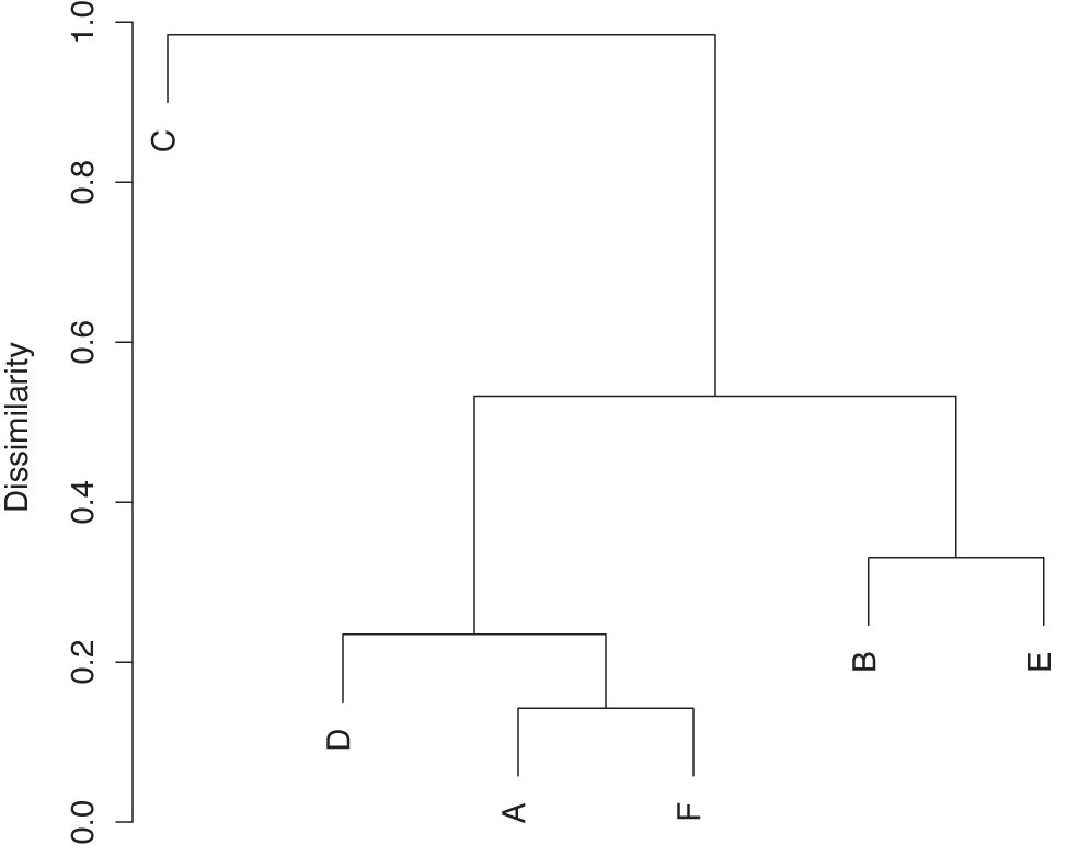
The result of hierarchical clustering is not actually a set of clusters. Instead, we obtain a treelike structure that contains the individual data points at the leaf nodes. This structure can be represented graphically in a dendrogram (see Figure 13-10). To extract actual clusters from it, we need to walk the tree, evaluate the cluster properties for each subtree, and then cut the tree to obtain clusters.
Tree builders are expensive: we need at least the full
distance matrix for all pairs of points (requiring
(n2)
operations to evaluate). Building the complete tree takes
(n) iterations: there are
n clusters (initially, points) to start with,
and at each iteration, the number of clusters is reduced by one
because two clusters are combined. For each iteration, we need to
search the distance matrix for the closest pair of clusters—naively
implemented, this is an (n2)
operation that leads to a total complexity of (n3)
operations. However, this can be reduced to (n2
log n) by using indexed lookup.
One outstanding feature of hierarchical clustering is that it does more than produce a flat list of clusters; it also shows their relationships in an explicit way. You need to decide whether this information is relevant for your needs, but keep in mind that the choice of measure for the cluster distance (single- or complete-link, and so on) can have a significant influence on the appearance of the resulting tree structure.
Neighborhood Growers
A third kind of clustering algorithm could be dubbed “neighborhood growers.” They work by connecting points that are “sufficiently close” to each other to form a cluster and then keep doing so until all points have been classified. This approach makes the most direct use of the definition of a cluster as a region of high density, and it makes no assumptions about the overall shape of the cluster. Therefore, such methods can handle clusters of complicated shapes (as in Figure 13-6), interwoven clusters, or even nested clusters (as in Figure 13-3). In general, neighborhood-based clustering algorithms are more of a special-purpose tool: either for cases that other algorithms don’t handle well (such as the ones just mentioned) or for polishing, in a second pass, the features of a cluster found by a general-purpose clustering algorithm such as k-means.
The DBSCAN algorithm which we will introduce in this section is one such algorithm, and it demonstrates some typical concepts. It requires two parameters. One is the minimum density that we expect to prevail inside of a cluster—points that are less densely packed will not be considered part of any cluster. The other parameter is the size of the region over which we expect this density to be maintained: it should be larger than the average distance between neighboring points but smaller than the entire cluster. The choice of parameters is rather subtle and clearly requires an appropriate balance.
In a practical implementation, it is easier to work with two slightly different parameters: the neighborhood radius r and the minimum number of points n that we expect to find within the neighborhood of each point in a cluster. The DBSCAN algorithm distinguishes between three types of points: noise, edge, and core points. A noise point is a point which has fewer than n points in its neighborhood of radius r, such a point does not belong to any cluster. A core point of a cluster has more than n neighbors. An edge point is a point that has fewer neighbors than required for a core point but that is itself the neighbor of a core point. The algorithm discards noise points and concentrates on core points. Whenever it finds a core point, the algorithm assigns a cluster label to that point and then continues to add all its neighbors, and their neighbors recursively to the cluster, until all points have been classified.
This description is simple enough, but actually deriving a concrete implementation that is both correct and efficient is less than straightforward. The pseudo-code in the original paper[22] appears needlessly clumsy; on the other hand, I am not convinced that the streamlined version that can be found (for example) on Wikipedia is necessarily correct. Finally, the basic algorithm lends itself to elegant recursive implementations, but keep in mind that the recursion will not unwind until the current cluster is complete. This means that, in the worst case (of a single connected cluster), you will end up putting the entire data set onto the stack!
As pointed out earlier, the main advantage of the DBSCAN algorithm is that it handles clusters of complicated shapes and nested clusters gracefully. However, it does depend sensitively on the appropriate choice of values for its two control parameters, and it provides little help in finding them. If a data set contains several clusters with widely varying densities, then a single set of parameters may not be sufficient to classify all of the clusters. These problems can be ameliorated by coupling the DBSCAN algorithm with the k-means algorithm: in a first pass, the k-means algorithm is used to identify candidates for clusters. Moreover, statistics on these subsets of points (such as range and density) can be used as input to the DBSCAN algorithm.
The DBSCAN algorithm is dominated by the calculations required
to find the neighboring points. For each point in the data set, all
other points have to be checked; this leads to a complexity of
(n2).
In principle, algorithms and data structures exist to find
candidates for neighboring points more efficiently
(e.g., kd-trees and global
grids), but their implementations are subtle and carry their own
costs (grids can be very memory intensive). Coupling the DBSCAN
algorithm with a more efficient first-pass algorithm (such as
k-means) may therefore be a better
strategy.
Pre- and Postprocessing
The core algorithm for grouping data points into clusters is usually only part (though the most important one) of the whole strategy. Some data sets may require some cleanup or normalization before they are suitable for clustering: that’s the first topic in this section.
Furthermore, we need to inspect the results of every clustering algorithm in order to validate and characterize the clusters that have been found. We will discuss some concepts and quantities used to describe clusters and to measure the clustering quality.
Finally, several cluster algorithms require certain input parameters (such as the number of clusters to find), and we need to confirm that the values we provided are consistent with the outcome of the clustering process. That will be our last topic in this section.
Scale Normalization
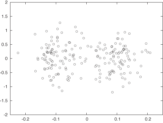
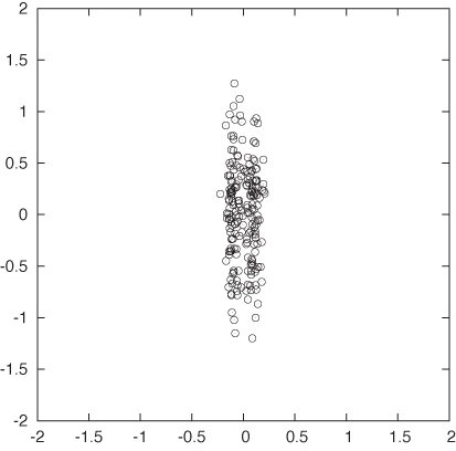
Look at Figure 13-11 and Figure 13-12. Wouldn’t you agree that the data set in Figure 13-11 exhibits two reasonably clearly defined and well-separated clusters while the data set in Figure 13-12 does not? Yet both figures show the same data set—only drawn to different scales! In Figure 13-12, I used identical units for both the x axis and the y axis; whereas Figure 13-11 was drawn to maintain a suitable aspect ratio for this data set.
This example demonstrates that clustering is not independent of the units in which the data is measured. In fact, for the data set shown in Figure 13-11 and Figure 13-12, points in two different clusters may be closer to each other than to other points in the same cluster! This is clearly a problem.
If, as in this example, your data spans very different ranges along different dimensions, you need to normalize the data before starting a clustering algorithm. An easy way to achieve this is to divide the data, dimension for dimension, by the range of the data along that dimension. Alternatively, you might want to divide by the standard deviation along that dimension. This process is sometimes called whitening or prewhitening, particularly in signal-theoretic literature.
You only need to worry about this problem if you are working with vector-like data and are using a distance measure like the Euclidean distance. It does not affect correlation-based similarity measures. In fact, there is a special variant of the Euclidean distance that performs the appropriate rescaling for each dimension on the fly: the Mahalanobis distance.
Cluster Properties and Evaluation
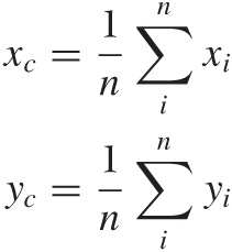
It is easiest to think about cluster properties in the context of vector-like data and a straightforward clustering algorithm such as k-means. The algorithm already gives us the coordinates of the cluster centroids directly, hence we have the cluster location. Two additional quantities are the mass of the cluster (i.e., the number of points in the cluster) and its radius. The radius is simply the average deviation of all points from the cluster center—basically the standard deviation, when using the Euclidean distance:
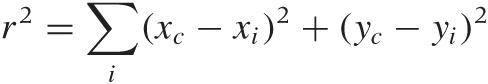
in two dimensions (equivalently in higher dimensions). Here xc and yc are the coordinates of the center of the cluster, and the sum runs over all points i in the cluster. Dividing the mass by the radius gives us the density of the cluster. (These values can be used to construct input values for the DBSCAN algorithm.)
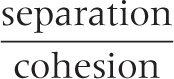
We can apply the same principles to develop a measure for the overall quality of the clustering. The key concepts are cohesion within a cluster and separation between clusters. The average distance for all points within one cluster is a measure of the cohesion, and the average distance between all points in one cluster from all points in another cluster is a measure of the separation between the two clusters. (If we know the centroids of the clusters, we can use the distance between the centroids as a measure for the separation.) We can go further and form the average (weighted by the cluster mass) of the cohesion for all clusters as a measure for the overall quality.
If a data set can be cleanly grouped into clusters, then we expect the distance between the clusters to be large compared to the radii of the clusters. In other words, we expect the ratio:
to be large.
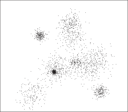
A particular measure based on this concept is the silhouette coefficient S. The silhouette coefficient is defined for individual points as follows. Let ai be the average distance (the cohesion) that point i has from all other points in the cluster to which it belongs. Evaluate the average distance that point i has from all points in any cluster to which it does not belong, and let bi be the smallest such value (i.e., bi is the separation from the “closest” other cluster). Then the silhouette coefficient of point i is defined as:
The numerator is a measure for the “empty space” between clusters (i.e., it measures the amount of distance between clusters that is not occupied by the original cluster). The denominator is the greater of the two length scales in the problem—namely the cluster radius and the distance between clusters.
By construction, the silhouette coefficient ranges from –1 to 1. Negative values indicate that the cluster radius is greater than the distance between clusters, so that clusters overlap; this suggests poor clustering. Large values of S suggest good clustering. We can form the average of the silhouette coefficients for all points belonging to a single cluster and thereby develop a measure for the quality of the entire cluster. We can further define the average over the silhouette coefficients for all individual points as the overall silhouette coefficient for the entire data set; this would be a measure for the quality of the clustering result.
The overall silhouette coefficient can be useful to determine the number of clusters present in the data set. If we run the k-means algorithm several times for different values of the expected number of clusters and calculate the overall silhouette coefficient each time, then it should exhibit a peak near the optimal number of clusters.
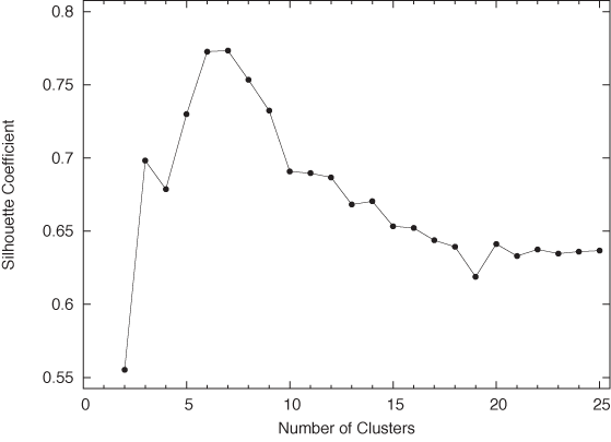
Let’s work through an example to see how the the silhouette coefficient performs in practice. Figure 13-13 shows the points of a two-dimensional data set. This is an interesting data set because, even though it exhibits clear clustering, it is not at all obvious how many distinct clusters there really are—any number between six and eight seems plausible. The total silhouette coefficient (averaged over all points in the data set) for this data set (see Figure 13-14) confirms this expectation, clearly leaning toward the lower end of this range. (It is interesting to note that the data set was generated, using a random-number generator, to include 10 distinct clusters, but some of those clusters are overlapping so strongly that it is not possible to distinguish them.) This example also serves as a cautionary reminder that it may not always be so easy to determine what actually constitutes a cluster!
Another interesting question concerns distinguishing legitimate clusters from a random (unclustered) background. Of the algorithms that we have seen, only the DBSCAN algorithm explicitly labels some points as background; the k-means and the tree-building algorithm perform what is known as complete clustering by assigning every point to a cluster. We may want to relax this behavior by trimming those points from each cluster that exceed the average cohesion within the cluster by some amount. This is easiest for fuzzy clustering algorithms, but it can be done for other algorithms as well.
Other Thoughts
The three types of clustering algorithms introduced in this chapter are probably the most popular and widely used, but they certainly don’t exhaust the range of possibilities.
Here is a brief list of other ideas that can (and have) been used to develop clustering algorithms.
We can impose a specific topology, such as a grid on the data points. Each data point will fall into a single grid cell, and we can use this information to find cells containing unusually many points and so guide clustering. Cell-based methods will perform poorly in many dimensions, because most cells will be empty and have few occupied neighbors (the “curse of dimensionality”).
Among grid-based approaches, Kohonen maps (which we will discuss in Chapter 14) have a lot of intuitive appeal.
Some special methods have been suggested to address the challenges posed by high-dimensional feature spaces. In subspace clustering, for example, clustering is performed on only a subset of all available features. These results are then successively extended by including features ignored in previous iterations.
Remember kernel density estimates (KDEs) from Chapter 2? If the dimensionality is not too high, then we can generate a KDE for the data set. The KDE provides a smooth approximation to the local point density. We can then identify clusters by finding the maxima of this density directly, using standard methods from numerical analysis.
The QT (“quality threshold”) algorithm is a center-seeking algorithm that does not require the number of clusters as input; instead, we have to fix a maximum radius. The QT algorithm treats every point in the cluster as a potential centroid and adds neighboring points (in the order of increasing distance from the centroid) until the maximum radius is exceeded. Once all candidate clusters have been completed in this way, the cluster with the greatest number of points is removed from the data set, and then the process starts again with the remaining points.
There is a well-known correspondence between graphs and distance matrices. Given a set of points, a graph tells us which points are directly connected to each other—but so does a distance matrix! We can exploit this equivalence by treating a distance matrix as the adjacency matrix of a graph. The distance matrix is pruned (by removing connections that are too long) to obtain a sparse graph, which can be interpreted as the backbone of a cluster.
Finally, spectral clustering uses powerful but abstract methods from linear algebra (similar to those used for principal component analysis; see Chapter 14) to structure and simplify the distance matrix.
Obviously, much depends on our prior knowledge about the data set: if we expect clusters to be simple and convex, then the k-means algorithm suggests itself. On the other hand, if we have a sense for the typical radius of the clusters that we expect to find, then QT clustering would be a more natural approach. If we expect clusters of complicated shapes or nested clusters, then an algorithm like DBSCAN will be required. Of course, it might be difficult to develop this kind of intuition—especially for problems that have significantly more than two or three dimensions!
Besides thinking of different ways to combine points into clusters, we can also think of different ways to define clusters to begin with. All methods discussed so far have relied (directly or indirectly) on the information contained in the distance between any two points. We can extend this concept and begin to think about three-point (or higher) distance functions. For example, it is possible to determine the angle between any three consecutive points and use this information as the measure of the similarity between points. Such an approach might help with cases like the one shown in Figure 13-8. Yet another idea is to measure not the similarity between points but instead the similarity between a point and a property of the cluster. For example, there is a straightforward generalization of the k-means algorithm in which the centroids are no longer pointlike but are straight lines, representing the “axis” of an elongated cluster. Rather than measuring the distance for each point from the centroid, this algorithm calculates the distance from this axis when assigning points to clusters. This algorithm would be suitable for cases like that shown in Figure 13-7. I don’t think any of these ideas that try to generalize beyond pairwise distances have been explored in detail yet.
A Special Case: Market Basket Analysis
Which items are frequently bought together? This and similar questions arise in market basket analysis or—more generally—in association analysis. Because association analysis is looking for items that occur together, it is in some ways related to clustering. However, the specific nature of the problem is different enough to require a separate toolset.
The starting point for association analysis is usually a data set consisting of transactions—that is, items that have been purchased together (we will often stay with the market basket metaphor when illustrating these concepts). Each transaction corresponds to a single “data point” in regular clustering.
For each transaction, we keep track of all items that have occurred together but typically ignore whether or not any particular item was purchased multiple times: all attributes are Boolean and indicate only the presence or absence of a certain item. Each item spans a new dimension: if the store sells N different items, then each transaction can have up to N different (Boolean) attributes, although each transaction typically contains only a tiny subset of the entire selection. (Note that we do not necessarily need to know the dimensionality N ahead of time: if we don’t know it, we can infer an approximation from the number of different items that actually occur in the data set.)
From this description, you can already see how association analysis differs from regular clustering: data points in association analysis are typically very high-dimensional but also very sparse. It also differs from clustering (as we have discussed it so far) in that we are not necessarily interested in grouping entire “points” (i.e., transactions) but would like to identify those dimensions that frequently occur together.
A group of zero or more items occurring together is known as an item set (or itemset). Each transaction consists of an item set, but every one of its subsets is also an item set. We can construct arbitrary item sets from the selection of available items. For each such item set, its support count is the number of actual transactions that contain the candidate item set as a subset.
Besides simply identifying frequent item sets, we can also try to derive association rules—that is, rules of the form “if items A and B are bought, then item C is also likely to be bought.” Two measures are important when evaluating the strength of an association rule: its support s and its confidence c. The support of a rule is the fraction of transactions in the entire data set that contain the combined item set (i.e., the fraction of transactions that contain all three items A, B, and C). A rule with low support is not very useful because it is rarely applicable.
The confidence is a measure for the reliability of an association rule. It is defined as the number of transactions in which the rule is correct, divided by the number of transactions in which it is applicable. In our example, it would be the number of times A, B, and C occur together divided by the number of times A and B occur together.
How do we go about finding frequent item sets (and association rules)? Rather than performing an open-ended search for the “best” association rule, it is customary to set thresholds for the minimum support (such as 10 percent) and confidence (such as 80 percent) required of a rule and then to generate all rules that meet these conditions.
To identify rules, we generate candidate item sets and then evaluate them against the set of transactions to determine whether they exceed the required thresholds. However, the naive approach—to create and evaluate all possible item sets of k elements—is not feasible because of the huge number (2k) of candidate item sets that could be generated, most of which will not be frequent! We must find a way to generate candidate item sets more efficiently.
The crucial observation is that an item set can occur frequently only if all of its subsets occur frequently. This insight is the basis for the so-called apriori algorithm, which is the most fundamental algorithm for association analysis.
The apriori algorithm is a two-step algorithm: in the first step, we identify frequent item sets; in the second step, we extract association rules. The first part of the algorithm is the more computationally expensive one. It can be summarized as follows.
Find all 1-item item sets that meet the minimum support threshold.

repeat:
  from the current list of k-item item sets, construct (k+1)-item item sets
  eliminate those item sets that do not meet the minimum support threshold
  stop when no (k+1)-item item set meets the minimum support threshold
The list of frequent item sets may be all that we require, or we may postprocess the list to extract explicit association rules. To find association rules, we split each frequent item set into two sets, and evaluate the confidence associated with this pair. From a practical point of view, rules that have a 1-item item set on the “righthand side” are the easiest to generate and the most important. (In other words, rules of the form “people who bought A and B also bought C,” rather than rules of the form “people who bought A and B also bought C and D.”)
This basic description leaves out many technical details, which are important in actual implementations. For example: how exactly do we create a (k + 1)-item item set from the list of k-item item sets? We might take every single item that occurs among the k-item item sets and add it, in turn, to every one of the k-item item sets; however, this would generate a large number of duplicate item sets that need to be pruned again. Alternatively, we might combine two k-item item sets only if they agree on all but one of their items. Clearly, appropriate data structures are essential for obtaining an efficient implementation. (Similar considerations apply when determining the support count of a candidate item set, and so on.)[23]
Although the apriori algorithm is probably the most popular algorithm for association analysis, there are also very different approaches. For example, the FP-Growth Algorithm (where FP stands for “Frequent Pattern”) identifies frequent item sets using something like a string-matching algorithm. Items in transactions are sorted by their support count, and a treelike data structure is built up by exploiting data sets that agree in the first k items. This tree structure is then searched for frequently occurring item sets.
Association analysis is a relatively complicated problem that involves many technical (as opposed to conceptual) challenges as well. The discussion in this section could only introduce the topic and attempt to give a sense of the kinds of approaches that are available. We will see some additional problems of a similar nature in Chapter 18.
A Word of Warning
Clustering can lead you astray, and when done carelessly it can become a huge waste of time. There are at least two reasons for this: although the algorithms are deceptively simple, it can be surprisingly difficult to obtain useful results from them. Many of them depend quite sensitively on several heuristic parameters, and you can spend hours fiddling with the various knobs. Moreover, because the algorithms are simple and the field has so much intuitive appeal, it can be a lot of fun to play with implementations and to develop all kinds of modifications and variations.
And that assumes there actually are any clusters present! (This is the second reason.) In the absence of rigorous, independent results, you will actually spend more time on data sets that are totally worthless—perpetually hunting for those clusters that “the stupid algorithm just won’t find.” Perversely, additional domain knowledge does not necessarily make the task any easier: knowing that there should be exactly 10 clusters present in Figure 13-13 is of no help in finding the clusters that actually can be identified!
Another important question concerns the value that you ultimately derive from clustering (assuming now that at least one of the algorithms has returned something apparently meaningful). It can be difficult to distinguish spurious results from real ones: like clustering algorithms, cluster evaluation methods are not particularly rigorous or unequivocal either (Figure 13-14 does not exactly inspire confidence). And we still have not answered the question of what you will actually do with the results—assuming that they turn out to be significant.
I have found that understanding the actual question that needs to be answered, developing some pertinent hypotheses and models around it, and then verifying them on the data through specific, focused analysis is usually a far better use of time than to go off on a wild-goose clustering search.
Finally, I should emphasize that, in keeping with the spirit of this book, the algorithms in this chapter are suitable for moderately sized data sets (a few thousand data points and a dozen dimensions, or so) and for problems that are not too pathological. Highly developed algorithms (e.g., CURE and BIRCH) exist for very large or very high-dimensional problems; these algorithms usually combine several different cluster-finding approaches together with a set of heuristics. You need to evaluate whether such specialized algorithms make sense for your situation.
Workshop: Pycluster and the C Clustering Library
The C Clustering Library (http://bonsai.hgc.jp/~mdehoon/software/cluster/software.htm) is a mature and relatively efficient clustering library originally developed to find clusters among gene expressions in microarray experiments. It contains implementations of the k-means and k-medoids algorithms, tree clustering, and even self-organized (Kohonen) maps. It comes with its own GUI frontend as well as excellent Perl and Python bindings. It is easy to use and very well documented. In this Workshop, we use Python to demonstrate the library’s center-seeker algorithms.
import Pycluster as pc
import numpy as np
import sys

# Read data filename and desired number of clusters from command line
filename, n = sys.argv[1], int( sys.argv[2] )

# x and y coordinates, whitespace-separated
data = np.loadtxt( filename, usecols=(0,1) )

# Perform clustering and find centroids
clustermap = pc.kcluster( data, nclusters=n, npass=50 )[0]
centroids = pc.clustercentroids( data, clusterid=clustermap )[0]

# Obtain distance matrix
m = pc.distancematrix( data )

# Find the masses of all clusters
mass = np.zeros( n )
for c in clustermap:
    mass[c] += 1

# Create a matrix for individual silhouette coefficients
sil = np.zeros( n*len(data) )
sil.shape = ( len(data), n )

# Evaluate the distance for all pairs of points
for i in range( 0, len(data) ):
    for j in range( i+1, len(data) ):
        d = m[j][i]

        sil[i, clustermap[j] ] += d
        sil[j, clustermap[i] ] += d

# Normalize by cluster size (that is: form average over cluster)
for i in range( 0, len(data) ):
    sil[i,:] /= mass

# Evaluate the silhouette coefficient
s = 0
for i in range( 0, len(data) ):
    c = clustermap[i]
    a = sil[i,c]
    b = min( sil[i, range(0,c)+range(c+1,n) ] )
    si = (b-a)/max(b,a) # This is the silhouette coeff of point i
    s += si

# Print overall silhouette coefficient
print n, s/len(data)
The listing shows the code used to generate Figure 13-14, showing how the silhouette coefficient depends on the number of clusters. Let’s step through it.
We import both the Pycluster
library itself as well as the NumPy package. We will use some of the
vector manipulation abilities of the latter. The point coordinates are
read from the file specified on the command line. (The file is assumed
to contain the x and y
coordinates of each point, separated by whitespace; one point per
line.) The point coordinates are then passed to the kcluster() function, which performs the
actual k-means algorithm. This function takes a
number of optional arguments: nclusters is the desired number of clusters,
and npass holds the number of
trials that should be performed with different
starting values. (Remember that k-means
clustering is nondeterministic with regard to the initial guesses for
the positions of the cluster centroids.) The kcluster() function will make npass different trials and report on the
best one.
The function returns three values. The first return value is an
array that, for each point in the original data set, holds the index
of the cluster to which it has been assigned. The second and third
return values provide information about the quality of the clustering
(which we ignore in this example). This function signature is a
reflection of the underlying C API, where you pass in an array of the
same length as the data array and then the cluster assignments of each
point are communicated via this additional array. This frees the
kcluster() function from having to
do its own resource management, which makes sense in C (and possibly
also for extremely large data sets).
All information about the result of the clustering procedure are
contained in the clustermap data
structure. The Pycluster library
provides several functions to extract this information; here we
demonstrate just one: we can pass the clustermap to the clustercentroids() function to obtain the
coordinates of the cluster centroids. (However, we won’t actually use
these coordinates in the rest of the program.)
You may have noticed that we did not specify the distance
function to use in the listing. The C Clustering Library does
not give us the option of a user-defined distance
function with k-means. It does include several
standard distance measures (Euclidean, Manhattan, correlation, and
several others), which can be selected through a keyword argument to
kcluster() (the default is to use
the Euclidean distance). Distance calculations can be a rather
expensive part of the algorithm, and having them implemented in C
makes the overall program faster. (If we want to define our own
distance function, then we have to use the kmedoids() function, which we will discuss
in a moment.)
To evaluate the silhouette coefficient we need the
point-to-point distances, and so we obtain the distance matrix from
the Pycluster library. We will also
need the number of points in each cluster (the cluster’s “mass”)
later.
Next, we calculate the individual silhouette coefficients for
all data points. Recall that the silhouette coefficient involves both
the average distance to the all points in the
same cluster as well as the average distance to
all points in the nearest cluster. Since we don’t
know ahead of time which one will be the nearest cluster to each
point, we simply go ahead and calculate the average distance to
all clusters. The results are stored in the
matrix sil.
(In the implementation, we make use of some of the vector
manipulation features of NumPy: in the expression sil[i,:] /= mass, each entry in row i is divided componentwise by the
corresponding entry in mass.
Further down, we make use of “advanced indexing” when looking for the
minimum distance between the point i and a cluster to which it does not belong:
in the expression b = min( sil[i,
range(0,c)+range(c+1,n) ] ), we construct an indexing vector
that includes indices for all clusters except the one that the point
i belongs to. See the Workshop in
Chapter 2 for more
details.)
Finally, we form the average over all single-point silhouette coefficients and print the results. Figure 13-14 shows them as a graph.
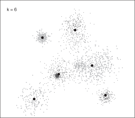
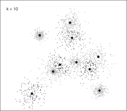
Figure 13-15 and Figure 13-16 show how the program assigned points to clusters in two runs, finding 6 and 10 clusters, respectively. These results agree with Figure 13-14: k = 6 is close to the optimal number of clusters, whereas k = 10 seems to split some clusters artificially.
The next listing demonstrates the kmedoids() function, which we have to use if
we want to provide our own distance function. As implemented by the
Pycluster library, the
k-medoids algorithm does not
require the data at all—all it needs is the distance matrix!
import Pycluster as pc
import numpy as np
import sys

# Our own distance function: maximum norm
def dist( a, b ):
    return max( abs(  a - b ) )

# Read data filename and desired number of clusters from command line
filename, n = sys.argv[1], int( sys.argv[2] )

# x and y coordinates, whitespace-separated
data = np.loadtxt( filename, usecols=(0,1) )
k = len(data)

# Calculate the distance matrix
m = np.zeros( k*k )
m.shape = ( k, k )

for i in range( 0, k ):
    for j in range( i, k ):
        d = dist( data[i], data[j] )
        m[i][j] = d
        m[j][i] = d

# Perform the actual clustering
clustermap = pc.kmedoids( m, n, npass=20 )[0]

# Find the indices of the points used as medoids, and the cluster masses
medoids =  {}
for i in clustermap:
    medoids[i] = medoids.get(i,0) + 1


# Print points, grouped by cluster
for i in medoids.keys():
    print "Cluster=", i, " Mass=", medoids[i], " Centroid: ", data[i]

    for j in range( 0, len(data) ):
        if clustermap[j] == i:
            print "\t", data[j]
In the listing, we calculate the distance matrix using the
maximum norm (which is not supplied by Pycluster) as distance function. Obviously,
we could use any other function here—such as the Levenshtein distance
if we wanted to cluster the strings in Figure 13-4.
We then call the kmedoids()
function, which returns a clustermap data structure similar to the one
returned by kcluster(). For the
kmedoids() function, the data
structure contains—for each data point—the index of the data point
that is the centroid of the assigned cluster.
Finally, we calculate the masses of the clusters and print the coordinates of the cluster medoids as well as the coordinates of all points assigned to that cluster.
The C Clustering Library is small and relatively easy to use. You might also want to explore its tree-clustering implementation. The library also includes routines for Kohonen maps and principal component analysis, which we will discuss in Chapter 14.
Further Reading
Introduction to Data Mining. Pang-Ning Tan, Michael Steinbach, and Vipin Kumar. Addison-Wesley. 2005.
This is my favorite book on data mining. The presentation is compact and more technical than in most other books on this topic. The section on clustering is particularly strong.
Data Clustering: Theory, Algorithms, and Applications. Guojun Gan, Chaoqun Ma, and Jianhong Wu. SIAM. 2007.
This book is a recent survey of results from clustering research. The presentation is too terse to be useful, but it provides a good source of concepts and keywords for further investigation.
Algorithms for Clustering Data. Anil K. Jain and Richard C. Dubes. Prentice Hall. 1988. An older book on clustering as freely available at http://www.cse.msu.edu/~jain/Clustering_Jain_Dubes.pdf.
Metric Spaces: Iteration and Application. Victor Bryant. Cambridge University Press. 1985. If you are interested in thinking about distance measures in arbitrary spaces in a more abstract way, then this short (100-page) book is a wonderful introduction. It requires no more than some passing familiarity with real analysis, but it does a remarkable job of demonstrating the power of purely abstract reasoning—both from a conceptual point of view but also with an eye to real applications.
[21] The Minkowski distance defined here should not be confused with the Minkowski metric, which defines the metric of the four-dimensional space-time in special relativity.
[22] “A Density-Based Algorithm for Discovering Clusters in Large Spatial Databases with Noise.” Martin Ester, Hans-Peter Kriegel, Jörg Sander, and Xiaowei Xu. Proceedings of 2nd International Conference on Knowledge Discovery and Data Mining (KDD-96). 1996.
[23] An open source implementation of the apriori algorithm (and
many other algorithms for frequent pattern identification),
together with notes on efficient implementation, can be found at
http://borgelt.net/apriori.html. The
arules package for R is an
alternative. It can be found on CRAN.