Table of Contents for
Data Analysis with Open Source Tools
 Data Analysis with Open Source Tools
Published by
O'Reilly Media, Inc., 2010
Data Analysis with Open Source Tools
Published by
O'Reilly Media, Inc., 2010
- Cover
- Data Analysis with Open Source Tools
- O'Reilly Strata Conference
- Data Analysis with Open Source Tools
- Dedication
- A Note Regarding Supplemental Files
- Preface
- 1. Introduction
- I. Graphics: Looking at Data
- 2. A Single Variable: Shape and Distribution
- 3. Two Variables: Establishing Relationships
- 4. Time As a Variable: Time-Series Analysis
- 5. More Than Two Variables: Graphical Multivariate Analysis
- 6. Intermezzo: A Data Analysis Session
- II. Analytics: Modeling Data
- 7. Guesstimation and the Back of the Envelope
- 8. Models from Scaling Arguments
- 9. Arguments from Probability Models
- 10. What You Really Need to Know About Classical Statistics
- 11. Intermezzo: Mythbusting—Bigfoot, Least Squares, and All That
- III. Computation: Mining Data
- 12. Simulations
- 13. Finding Clusters
- 14. Seeing the Forest for the Trees: Finding Important Attributes
- 15. Intermezzo: When More Is Different
- IV. Applications: Using Data
- 16. Reporting, Business Intelligence, and Dashboards
- 17. Financial Calculations and Modeling
- 18. Predictive Analytics
- 19. Epilogue: Facts Are Not Reality
- A. Programming Environments for Scientific Computation and Data Analysis
- B. Results from Calculus
- C. Working with Data
- D. About the Author
- Index
- About the Author
- Colophon
- Copyright
Chapter 17. Financial Calculations and Modeling
I RECENTLY RECEIVED A NOTICE FROM A MAGAZINE REMINDING ME THAT MY SUBSCRIPTION WAS RUNNING OUT. It’s a relatively expensive weekly magazine, and they offered me three different plans to renew my subscription: one year (52 issues) for $130, two years for $220, or three years for $275. Table 17-1 summarizes these options and also shows the respective cost per issue.
Subscription | Total price | Price per issue |
Single issue | n/a | 6.00 |
1 year | 130 | 2.50 |
2 years | 220 | 2.12 |
3 years | 275 | 1.76 |
Assuming that I want to continue the subscription, which of these three options makes the most sense? From Table 17-1, we can see that each issue of the magazine becomes cheaper as I commit myself to a longer subscription period, but is this a good deal? In fact, what does it mean for a proposal like this to be a “good deal”? Somehow, stomping up nearly three hundred dollars right now seems like a stretch, even if I remind myself that it saves me more than half the price on each issue.
This little story demonstrates the central topic of this chapter: the time value of money, which expresses the notion that a hundred dollars today are worth more than a hundred dollars a year from now. In this chapter, I shall introduce some standard concepts and calculational tools that are required whenever we need to make a choice between different investment decisions—whether they involve our own personal finances or the evaluation of business cases for different corporate projects.
I find the material in this chapter fascinating—not because it is rocket science (it isn’t) but because it is so fundamental to how the economy works. Yet very few people, in particular, very few tech people, have any understanding of it. (I certainly didn’t.) This is a shame, not just because the topic is obviously important but also because it is not really all that mystical. A little familiarity with the basic concepts goes a long way toward removing most of the confusion (and, let’s face it, the intimidation) that many of us experience when reading the Wall Street pages.
More important in the context of this book is that a lot of data analysis is done specifically to evaluate different business proposals and to support decisions among them. To be able to give effective, appropriate advice, you want to understand the concepts and terminology of this particular problem domain.
The Time Value of Money
Let’s return to the subscription problem. The essential insight is that—instead of paying for the second and third year of the subscription now—I could invest that money, reap the investment benefit, and pay for the subsequent years of the subscription later. In other words, the discount offered by the magazine must be greater than the investment income I can expect if I were instead to invest the sum.
It is this ability to gain an investment benefit that makes having money now more valuable than having the same amount of money later. Note well that this has nothing to do with the concept of inflation, which is the process by which a certain amount of money tends to buy a lesser amount of goods as time passes. For our purposes, inflation is an external influence over which we have no control. In contrast, investment and purchasing decisions (such as the earlier magazine subscription problem) are under our control, and time value of money calculations can help us make the best possible decisions in this regard.
A Single Payment: Future and Present Value
Things are easiest when there is only a single payment involved. Imagine we are given the following choice: receive $1,000 today, or receive $1,050 a year from now. Which one should we choose?
Well, that depends on what we could do with $1,000 right now. For this kind of analysis, it is customary to assume that we would put the money in a “totally safe form of investment” and use the returns generated in this way as a benchmark for comparison.[28] Now we can compare the alternatives against the interest that would be generated by this “safe” investment. For example, assume that the current interest rate that we could gain on a “safe” investment is 5 percent annually. If we invest $1,000 for a full year, then at the year’s end, we will receive back our principal ($1,000) and, in addition, the accrued interest (0.05 · $1000 = $50), for a total of $1,050.
In this example, both options lead to the same amount of money after one year; we say that they are equivalent. In other words, receiving $1,000 now is equivalent to receiving $1,050 a year from now, given that the current interest rate on a safe form of investment is 5 percent annually. Equivalence always refers to a specific time frame and interest rate.
Clearly, any amount of money that we now possess has a future value (or future worth) at any point in the future; likewise, a payment that we will receive at some point in the future has a present value (or present worth) now. Both values depend on the interest rate that we could achieve by investing in a safe alternative investment instead. The present or future values must be equivalent at equal times.
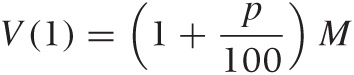
There is a little bit of math behind this that is not complicated but is often a little messy. The future value Vf of some base amount M (the principal), after a single time period during which the amount earns p percent of interest, is calculated as follows:
The first term on the righthand side expresses that we get our principal back, and the second term is the amount of interest we receive in addition. Here and in what follows, I explicitly show the denominator 100 that is used to translate a statement such as “p percent” into the equivalent numerical factor p/100.
Conversely, if we want to know how much a certain amount of money in the future is worth today, then we have to discount that amount to its present value. To find the present value, we work the preceding equation backward. The present value Vp is unknown, but we do know the amount of money M that we will have at some point in the future, hence the equation becomes:
This can be solved for Vp:
Note how we find the future or present value by multiplying the base amount by an appropriate equivalencing factor—namely, the future-worth factor 1 + p/100 and the present-worth factor 1/(1 + p/100). Because most such calculations involve discounting a future payment to the present value, the percentage rate p used in these formulas is usually referred to as the discount rate.
This example was the simplest possible because there was only a single payment involved—either at the beginning or at the end of the period under consideration. Next, we look at scenarios where there are multiple payments occurring over time.
Multiple Payments: Compounding
Matters become a bit more complicated when there is not just a single payment involved as in the example above but a series of payments over time. Each of these payments must be discounted by the appropriate time-dependent factor, which leads us to cash-flow analysis. In addition, payments made or received may alter the base amount on which we operate, this leads to the concept of compounding.
Let’s consider compounding first, since it is so fundamental. Again, the idea is simple: if we put a sum of money into an interest-bearing investment and then reinvest the generated interest, we will start to receive interest on the interest itself. In other words, we will start receiving compound interest.
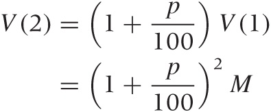
Here is how it works: we start with principal M and invest it at interest rate p. After one year, we have:
In the second year, we receive interest on the combined sum of the principal and the interest from the first year:
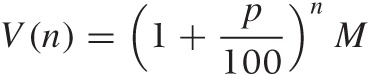
and so on. After n years, we will have:
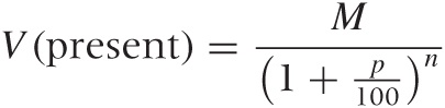
These equations tell us the future worth of our investment at any point in time. It works the other way around, too: we can determine the present value of a payment that we expect to receive n years from now by working the equations backward (much as we did previously for a single payment) and find:
We can see from these equations that, if we continue to reinvest our earnings, then the total amount of money grows exponentially with time (i.e., as at for some constant a)—in other words, fast. The growth law that applies to compound interest is the same that describes the growth of bacteria cultures or similar systems, where at each time step new members are added to the population and start producing offspring themselves. In such systems, not only does the population grow, but the rate at which it grows is constantly increasing as well.
On the other hand, suppose you take out a loan without making payments and let the lender add the accruing interest back onto your principal. In this case, you not only get deeper into debt every month, but you do so at a faster rate as time goes by.
Calculational Tricks with Compounding
Here is a simple trick that is quite convenient when making
approximate calculations of future and present worth. The
single-payment formula for future worth, V = (1
+ p/100)M, is simple and
intuitive: the principal plus the interest
after one period. In contrast, the corresponding formula for present
worth 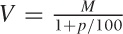 , seems to make less intuitive sense and is
harder to work with (how much is $1,000 divided by 1.05?). But this
is again one of those situations where guesstimation techniques (see
Chapter 7; also
see Appendix B) can be brought to
bear. We can approximate the discounting factor as follows:
, seems to make less intuitive sense and is
harder to work with (how much is $1,000 divided by 1.05?). But this
is again one of those situations where guesstimation techniques (see
Chapter 7; also
see Appendix B) can be brought to
bear. We can approximate the discounting factor as follows:
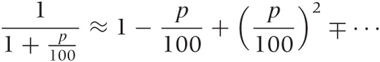
Since p is typically small (single digits), it follows that p/100 is very small, and so we can terminate the expansion after the first term. Using this approximation, the discounting equation for the present worth becomes V = (1 – p/100)M, which has an intuitive interpretation: the present value is equal to the future value, less the interest that we will have received by then.
We can use similar formulas even in the case of compounding, since:
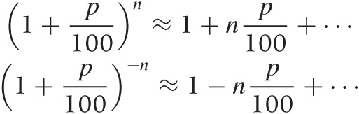
However, keep in mind that the overall perturbation must be small for the approximation to be valid. In particular, as the number of years n grows, the perturbation term np/100 may no longer be small. Still, even for 5 percent over 5 years, the approximation gives 1 ± 25/100 = 1.25 or 0.75, respectively. Compare this with the exact values of 1.28 and 0.79. However, for 10 percent over 10 years, the approximation starts to break down, yielding 2 and 0, respectively, compared to the exact values of 2.59 and 0.39.
Similar logic is behind “Einstein’s Rule of 72.” This rule of thumb states that if you divide 72 by the applicable interest rate, you obtain the number of years it would take for your investment to double. So if you earn 7 percent interest, your money will double in 10 years, but if you only earn 3.5 percent, it will take 20 years to double.
What’s the basis for this rule? By now, you can probably figure it out yourself, but here is the solution in a nutshell: for your investment to double, the compounding factor must equal 2. Therefore, we need to solve (1 + p/100)n = 2 for n. Applying logarithms on both sides we find n = log(2)/log(1 + p/100). In a second step, we expand the logarithm in the denominator (remember that p/100 is a small perturbation!) and end up with n = log(2) · (100/p) = 69/p, since the value of log(2) is approximately 0.69. The number 69 is awkward to work with, so it is usually replaced by the number 72—which has the advantage of being evenly divisible by 2, 3, 4, 6, 8, and 9 (you can replace 72 with 70 for interest rates of 5 or 7 percent).
Here is another calculational tool that you may find useful. Strictly speaking, an expression such as xn is defined only for integer n. For general exponents, the power function is defined as xn = exp(n log x). We can use this when calculating compounding factors as follows:
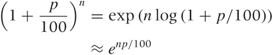
where in the second step we have expanded the logarithm again and truncated the expansion after the first term. This form of the compounding factor is often convenient (e.g., it allows us to use arbitrary values for the time period n, not just full years). It becomes exact in the limit of continuous compounding (discussed shortly).
Interest rates are conventionally quoted “per year,” as in “5 percent annually.” But payments may occur more frequently than that. Savings accounts, for example, pay out any accrued interest on a monthly basis. That means that (as long as we don’t withdraw anything) the amount of money that earns us interest grows every month; we say it is compounded monthly. (This is in contrast to other investments, which pay out interest or dividends only on a quarterly or even annual basis.) To take advantage of the additional compounding, it is of course in our interest (pun intended) to receive payments as early as possible.
This monthly compounding is the reason for the difference between the nominal interest rate and the annual yield that you will find stated on your bank’s website: the nominal interest rate is the rate p that is used to determine the amount of interest paid out to you each month. The yield tells you by how much your money will grow over the course of the year when the monthly compounding has been factored in. With our knowledge, we can now calculate the yield from the nominal rate:
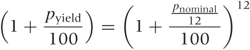
One more bit of terminology: the interest rate p/12 that is used to determine the value of the monthly payout is known as the effective interest rate.
Of course, other payment periods are possible. Many mutual funds pay out quarterly. In contrast, many credit cards compound daily. In theory, we can imagine payments being made constantly (but at an appropriately reduced effective interest rate); this is the case of continuous compounding mentioned earlier. In this case, the compounding factor is given by the exponential function. (Mathematically, you replace the 12 in the last formula by n and then let n go to infinity, using the identity limn→∞(1 + x/n)n = exp(x).)
The Whole Picture: Cash-Flow Analysis and Net Present Value
We now have all the tools at our disposal to evaluate the financial implications of any investment decision, no matter how complicated. Imagine we are running a manufacturing plant (or perhaps an operation like Amazon’s, where books and other goods are put into boxes and mailed to customers—that’s how I learned about all these things). We may consider buying some piece of automated equipment for some part of the process (e.g., a sorting machine that sorts boxes onto different trucks according to their destination). Alternatively, we can have people do the same job manually. Which of these two alternatives is better from an economic point of view?
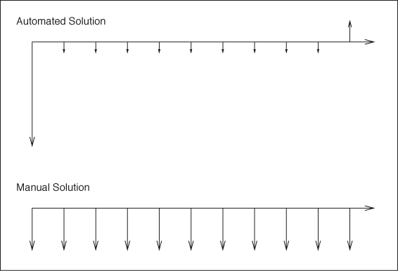
The manual solution has a simple structure: we just have to pay out the required wages every year. If we decide to buy the machine, then we have to pay the purchase price now (this is also known as the first cost) and also pay a small maintenance fee each year. For the sake of the argument, assume also that we expect to use the machine for ten years and then sell it on for scrap value.
In economics texts, you will often find the sequence of payments visualized using cash-flow diagrams (see Figure 17-1). Time progresses from left to right; inflows are indicated by upward-pointing arrows and outflows by downward-pointing arrows.
To decide between different alternatives, we now proceed as follows:
Determine all individual net cash flows (net cash flows, because we offset annual costs against revenues).
Discount each cash flow to its present value.
Add up all contributions.
The quantity obtained in the last step is known either as the net present value (NPV) or the discounted net cash flow: it is the total value of all cash flows, each properly discounted to its present value. In other words, our financial situation will be the same, whether we execute the entire series of cash flows or receive the net present value today. Because the net present value contains all inflows and outflows (properly discounted to the present value), it is a comprehensive single measure that can be used to compare the financial outcomes of different investment strategies.
We can express the net present value of a series of cash flows in a single formula:
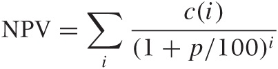
where c(i) is the net cash flow at payment period i and 1/(1 + p/100)i is the associated discounting factor.
There is one more concept that is interesting in this context. What should we use for the discount rate p in the second step above? Instead of supplying a value, we can ask how much interest we would have to receive elsewhere (on a “safe” investment) to obtain the same (or higher) payoff than that expected from the planned project. Let’s consider an example. Assume we are evaluating a project that would require us to purchase some piece of equipment at the beginning but that would then result in a series of positive cash flows over the next so many years. Is this a “good” investment? It is if its net present value is positive! (That’s pretty much the definition of “net present value”: the NPV takes into account the first cost to purchase the equipment as well as the subsequent positive cash flows. If the discounted cash flows are greater than the first cost, we come out ahead.) But the net present value depends on the discount rate p, so we need to find that value of p for which the NPV first becomes zero: if we can earn a higher interest rate elsewhere, then the project does not make financial sense and we should instead take our money to the bank. But if the bank would pay us less than the rate of return just calculated, then the project is financially the better option. (To find a numeric value for the rate of return, plug your cash flow structure c(i) into the equation for NPV and then solve for p. Unless the cash flows are particularly simple, you will have to do this numerically.)
The net present value is such an important criterion when making investment decisions because it provides us with a single number that summarizes the financial results of any planned project. It gives us an objective (financial) quantity to decide among different investment alternatives.
Up to a point, that is. The process described here is only as good as its inputs. In particular, we have assumed that we know all inputs perfectly—possibly for many years into the future. Of course we don’t have perfect knowledge, and so we better accommodate for that uncertainty somehow. That will be the topic of the next section.
There is another, more subtle problem when evaluating different options solely based on net present value: different investment alternatives may have nonfinancial benefits or drawbacks that are not captured by the net present value. For example, using manual labor may lead to greater flexibility: if business grows more strongly than expected, then the company can hire additional workers, and if business slows down, then it can reduce the number of workers. In contrast, any piece of equipment has a maximum capacity, which may be a limiting factor if business grows more strongly than expected. The distinction arising here is that between fixed and variable cost, and we will come back to it toward the end of the chapter.
Uncertainty in Planning and Opportunity Costs
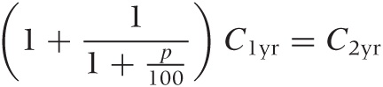
Now we are ready to revisit the magazine subscription problem from the beginning of this chapter. Let’s consider only two alternatives: paying the entire amount for a two-year subscription up front or making two single-year payments. The NPV for the second option is (1 + 1/(1 + p/100)) C1yr, where we have left the discount rate p undetermined for the moment. We can now ask: what interest rate would we have to earn elsewhere to make the second option worthwhile? In other words, we want to know the discount rate we’d have to apply to make the NPV of the multiple-payment option equal to the cost of the single-payment plan:
This equation can be solved for p. The result is p = 30 percent! In other words, the two-year subscription is so much cheaper that we would have to find an investment yielding 30 percent annually before it would be worthwhile to pay for the subscription year by year and invest the saved money elsewhere. No investment (and certainly no “safe” investment) yields anywhere near that much. Clearly, something is amiss. (Exercise for the reader: find the net present value for the three-year subscription and verify that it leads to the same value for p.)
Using Expectation Values to Account for Uncertainty
The two- and three-year plans carry a hidden cost for us: once we have signed up, we can no longer freely decide over our money—we’re committed ourselves for the long haul. In contrast, if we pay on a yearly basis, then we can reevaluate every year whether we want to continue the subscription. The price for this freedom is a higher subscription fee. However, we will probably not find it easy to determine the exact dollar value that this freedom is worth to us.
From the magazine’s perspective, the situation is simpler. They can simply ask how much money they expect to make from an individual subscriber under either option. If I sign up for the two-year subscription, they make C2yr with certainty; if I sign up for the one-year subscription, they make C1yr with certainty now and another C1yr later—provided I renew my subscription! In this case, then, the amount of money the magazine expects to make on me is C1yr + γC1yr, where γ is the probability that I will renew the subscription. From the magazine’s perspective, both options must be equally favorable (otherwise they would adjust the price of the two-year subscription to make them equal), so we can equate the expected revenues and solve for γ. The result comes out to about γ = 0.7—in other words, the magazine expects (based on past experience, and so on) that about 70 percent of its current subscribers will renew their subscription. For three years, the equation becomes (1 + γ + γ2)C1yr = C3yr because, to sign up for three years, a subscriber must decide twice to renew the subscription. If you work through the algebra, you will find that γ again comes out to about γ = 0.7, providing a nice consistency check.
There are two takeaways in this example that are worth emphasizing: the first concerns making economic decisions that are subject to uncertainty. The second is the concept of opportunity cost, which is the topic of the following section.
When making economic decisions that are subject to uncertainty, you may want to take this uncertainty into account by replacing the absolute cash flows with their expected values. A simple probability model for the likely payout is often sufficient. In the magazine example there were just two outcomes: the subscriber renews with probability γ = 0.7 and value C1yr, or the subscriber does not renew with probability γ = 0.3 and value 0, hence the expected value is 0.3 · 0 + 0.7 · C1yr. If your situation warrants it and if you can specify the probability distribution for various payout alternatives in more detail, then you can calculate the expected value accordingly. (See Chapter 8 and Chapter 9 for more information on how to build models to support this kind of conclusion.)
Working with expectation values is convenient, because once you have determined the expected value of the payout, you no longer need to worry about the probabilities for the various outcomes: they have been entirely absorbed into the expectation values. What you lose is insight into the probable spread of outcomes. For a quick order-of-magnitude check, that’s acceptable, but for a more serious study, an estimate of the spread should be included. There are two ways to do this: repeat your calculation multiple times using different values (low, medium, high) for the expected payouts at every step to develop a sense for the range of possible outcomes. (If there are many different options, you may want to do this through simulation; see Chapter 12.) Alternatively, you can evaluate both the expectation value and the spread directly from the probability distribution to obtain a range for each estimated value: μ ± σ. Now you can use this sum in your calculations, treating σ as a small perturbation and evaluate the effect of this perturbation on your model (see Chapter 7).
Opportunity Costs
The second point that I would like to emphasize is the concept of opportunity cost. Opportunity costs arise when we miss out on some income (the “opportunity”) because we were not in a position to take advantage of it. Opportunity costs formalize the notion that resources are finite and that, if we apply them to one purpose, then those resources are not available for other uses. In particular, if we commit resources to a project, then we want that project to generate a benefit greater than the opportunity costs that arise, because those resources are no longer available for other uses.
I find it easiest to think about opportunity cost in the context of certain business situations. For instance, suppose a company takes on a project that pays $15,000. While this contract is under way, someone else offers the company a project that would pay $20,000. Assuming that the company cannot break its initial engagement, it is now incurring an opportunity cost of $5,000.
I find the concept of opportunity cost useful as a way to put a price on alternatives, particularly when no money changes hands. In textbooks, this is often demonstrated by the example of the student who takes a trip around the world instead of working at a summer job. Not only does the student have to pay the actual expenses for the trip but also incurs an opportunity cost equal to the amount of forgone wages. The concept of opportunity cost allows us to account for these forgone wages, which would otherwise be difficult because they do not show up on any account statement (since they were never actually paid).
On the other hand, I often find opportunity cost a somewhat shadowy concept because it totally hinges on a competing opportunity actually arising. Imagine you try to decide between two opportunities: an offer for a project that would pay $15,000 and the prospect of a project paying $20,000. If you take the first job and then the second opportunity comes through as well, you are incurring an opportunity cost of $5,000. But if the second project falls through, your opportunity cost just dropped to zero! (The rational way to make this decision would be to calculate the total revenue expected from each prospect but weighted by the probability that the contract will actually be signed. This brings us back to calculations involving expected payouts, as discussed in the preceding section.)
To be clear: the concept of opportunity cost has nothing to do with uncertainty in planning. It is merely a way to evaluate the relative costs of competing opportunities. However, when evaluating competing deals, we must often decide between plans that have a different likelihood of coming to fruition, and therefore opportunity cost and planning for uncertainty often arise together.
Cost Concepts and Depreciation
The methods described in the previous sections might suggest that the net present value is all there is to financial considerations. This is not so—other factors may influence our decision. Some factors are entirely outside the financial realm (e.g., ethical or strategic considerations); others might have direct business implications but are not sufficiently captured by the quantities we have discussed so far.
For example, let’s go back to the situation discussed earlier where we considered the choice between two alternatives: buying a sorting machine or having the same task performed manually. Once we identify all arising costs and discount them properly to their present value, it would seem we have accounted for all financial implications. But that would be wrong: the solution employing manual labor is more flexible, for instance. If the pace of the business varies over the course of the year, then we need to buy a sorting machine that is large enough to handle the busiest season—which means it will be underutilized during the rest of the year. If we rely on manual labor, then we can more flexibly scale capacity up through temporary labor or overtime—and we can likewise respond to unexpectedly strong (or weak) growth of the overall business more flexibly, again by adjusting the number of workers. (This practice may have further consequences—for example, regarding labor relations.) In short, we need to look at the costs, and how they arise, in more detail.
To understand the cost structure of a business or an operation better, it is often useful to discuss it in terms of three pairs of complementary concepts:
Direct versus indirect cost
Fixed versus variable cost
Capital expenditure versus operating cost
For good measure, I’ll also throw in the concept of depreciation, although it is not a cost in the strict sense of the word.
Direct and Indirect Costs
Labor and materials that are applied in creating the product (i.e., in the creation of something the company will sell) are considered direct labor or direct materials cost. Indirect costs, on the other hand, arise from activities that the company undertakes to maintain itself: management, maintenance, and administrative tasks (payroll and accounting) but also training, for example. Another term for such indirect costs is overhead.
I should point out that this is a slightly different definition of direct and indirect costs than the one you will find in the literature. Most textbooks define direct cost as the cost that is “easily attributable” to the production process, whereas indirect cost is “not easily attributable.” This definition makes it seem as if the distinction between direct and indirect costs is mostly one of convenience. Furthermore, the textbook definition provides no reason why, for example, maintenance and repair activities are usually considered indirect costs. Surely, we can keep track of which machine needed how much repair and therefore assign the associated cost to the product made on that specific machine. On the other hand, by my definition, it is clear that maintenance should be considered an indirect cost because it is an activity the company undertakes to keep itself in good order—not to generate value for the customer.
I have used the term “product” for whatever the company is selling. For manufacturing or retail industries this is a straightforward concept, but for a service industry the “product” may be intangible. Nevertheless, in probably all businesses we can introduce the concept of a single produced unit or unit of production. In manufacturing and retail there are actual “units,” but in other industries the notion of a produced unit is a bit more artificial: in service industries, for instance, one often uses “billable hours” as a measure of production. Other industries have specialized conventions: the airline industry uses “passenger miles,” for example.
The unit is an important concept because it is the basis for the most common measure of productivity—namely the unit cost or cost per unit (CPU). The cost per unit is obtained by dividing the total (dollar) amount spent during a time period (per month, for instance) by the total number of units produced during that time. If we include not only the direct cost but also the indirect cost in this calculation, we obtain what is called the loaded or burdened cost per unit.
We can go further and break out the various contributions to the unit cost. For example, if there are multiple production steps, then we can determine how much each step contributes to the total cost. We can also study how much indirect costs contribute to the overall cost as well as how material costs relate to labor. Understanding the different contributions to the total cost per unit is often a worthwhile exercise because it points directly to where the money is spent. And appearances can be deceiving. I have seen situations where literally hundreds of people were required for a certain processing step whereas, next door, a single person was sufficient to oversee a comparable but highly automated process. Yet once you calculated the cost per unit, it all looked very different: because the number of units going through the automated process was low, its total cost per unit was actually higher than for the manual process. And because so many units where processed manually, their labor cost per unit turned out to be very low.
In general, it is desirable to have low overhead relative to the direct cost: a business should spend relatively less time and money on managing itself than on generating value for the customer. In this way, the ratio of direct to indirect cost can be a telling indicator for “top-heavy” organizations that seem mostly occupied with managing themselves. On the other hand, overeager attempts to improve the direct/indirect cost ratio can lead to pretty unsanitary manipulations. For example, imagine a company that considers software engineers direct labor, while any form of management (team leads and project managers) is considered indirect. The natural consequence is that management responsibilities are pushed onto developers to avoid “indirect” labor. Of course, this does not make these tasks go away; they just become invisible. (It also leads to the inefficient use of a scarce resource: developers are always in short supply—and they are expensive.) In short, beware the danger of perverted incentives!
Fixed and Variable Costs
Compared to the previous distinction (between direct and indirect costs), the distinction between fixed and variable costs is clearer. The variable costs are those that change in response to changing demand, while fixed costs don’t. For a car manufacturer, the cost of steel is a variable cost: if fewer cars are being built, less steel is consumed. Whether labor costs are fixed or variable depends on the type of labor and the employment contracts. But the capital cost for the machines in the production line is a fixed cost, because it has to be paid regardless of whether the machines are busy or idle.
It is important not to confuse direct and variable costs. Although direct costs are more likely to be variable (and overhead, in general, is fixed), these are unrelated concepts; one can easily find examples of fixed, yet direct costs. For example, consider a consultancy with salaried employees: their staff of consultants is a direct cost, yet it is also a fixed cost because the consultants expect their wages regardless of whether the consultancy has projects for them or not. (We’ll see another example in a moment.)
In general, having high fixed costs relative to variable ones makes a business or industry less flexible and more susceptible to downturns. An extreme example is the airline industry: its cost structure is almost exclusively fixed (pretty much the only variable cost is the price of the in-flight meal), but its demand pattern is subject to extreme cyclical swings.
The numbers are interesting. Let’s do a calculation in the spirit of Chapter 7. A modern jet airplane costs about $100M new and has a useful service life of about 10 years. The cost attributable to a single 10-hour transatlantic flight (the depreciation—see below) comes to about $30k (i.e., $100M/(10 · 365)—half that, if the plane is turned around immediately, completing a full round-trip within 24 hours). Fuel consumption is about 6 gallons per mile; if we assume a fuel price of $2 per gallon, then the 4,000-mile flight between New York and Frankfurt (Germany) will cost $50k for fuel. Let’s say there are 10 members of the cabin crew at $50k yearly salary and two people in the cockpit at $150k each. Double these numbers for miscellaneous benefits, and we end up with about $2M in yearly labor costs, or $10k attributable to this one flight. In contrast, the cost of an in-flight meal (wholesale) is probably less than $10 per person. For a flight with 200 passengers, this amounts to $1,000–2,000 dollars total. It is interesting to see that—all things considered—the influence of the in-flight meal on the overall cost structure of the flight is as high as it is: about 2 percent of the total. In a business with thin margins, improving profitability by 2 percent is usually seen as worthwhile. In other words, we should be grateful that we get anything at all! A final cross-check: the cost per passenger for the entire flight from the airline’s point of view is $375—and at the time of this writing, the cheapest fare I could find was $600 round-trip, equivalent to $300 for a single leg. As is well known, airlines break even on economy class passengers but don’t make any profits.
Capital Expenditure and Operating Cost
Our final distinction is the one between capital expenditure (CapEx) and operating expense (OpEx—the abbreviation is rarely used). Capital expenses are money spent to purchase long-lived and typically tangible assets: equipment, installations, real estate. Operating expenses are everything else: payments for rents, raw materials, fees, salaries. In most companies, separate budgets exist for both types of expense, and the availability of funds may be quite different for each. For example, in a company that is financially strapped but does have a revenue stream, it might be quite acceptable to hire and “throw people” at a problem (even at great cost), but it might very well be impossible to buy a piece of equipment that would take care of the problem for good. Conversely, in companies that do have money in the bank, it is often easier to get a lump sum approved for a specific purchase than to hire more people or to perform maintenance. Decision makers often are more inclined to approve funding for an identifiable and visible purchase than for spending money on “business as usual.” Political and vanity considerations may play a role as well.
The distinction between CapEx and operating costs is important because, depending on the availability of funds from either source, different solutions will be seen as feasible. (I refer to such considerations as “color of money” issues—although all dollars are green, some are greener than others!)
In the context of capital expenditure, there is one more concept that I’d like to introduce because it provides an interesting and often useful way of thinking about money: the notion of depreciation.[29] The idea is this: any piece of equipment that we purchase will have a useful service life. We can now distribute the total cost of that purchase across the entire life of the asset. For example, if I purchase a car for $24,000 and expect to drive it for 10 years, then I can say that this car costs me $200 per month “in depreciation” alone and before taking into account any operating costs (such as gas and insurance). I may want to compare this number with monthly lease payment options on the same kind of vehicle.
In other words, depreciation is a formalized way of capturing how an asset loses value over time. There are different standard ways to calculate it: “straight-line” distributes the purchase cost (less any salvage value that we might expect to obtain for the asset at the end of its life) evenly over the service life. The “declining balance” method assumes that the asset loses a certain constant fraction of its value every year. And so on. (Interestingly, land is never depreciated—because it does not wear out in the way a machine does and therefore does not have a finite service life.)
I find depreciation a useful concept, because it provides a good way to think about large capital expenses: as an ongoing cost rather than as an occasional lump sum. But depreciation is just that: a way of thinking. It is important to understand that depreciation is not a cash flow and therefore does not show up in any sort of financial accounting. What’s in the books is the money actually spent, when it is spent.
The only occasion where depreciation is treated as a cash flow is when it comes to taxes. The IRS (the U.S. tax authority) requires that certain long-lived assets purchased for business purposes be depreciated over a number of years, with the annual depreciation counted as a business expense for that year. For this reason, depreciation is usually introduced in conjunction with tax considerations. But I find the concept more generally useful as a way to think about and account for the cost of assets and their declining value over time.
Should You Care?
What does all this talk about money, business plans, and investment decisions have to do with data analysis? Why should you even care?
That depends. If you take a purely technical stance, then all of these questions are outside your area of competence and responsibility. That’s a valid position to take, and many practitioners will make exactly that decision.
Personally, I disagree. I don’t see it as my job to provide answers to questions. I see it as my responsibility to provide solutions to problems, and to do this effectively, I need to understand the context in which questions arise, and I need to understand how answers will be evaluated and used. Furthermore, when it comes to questions having to do with abstract topics like data and mathematical modeling, I have found that few clients are in a good position to ask meaningful questions. Coaching the client on what makes a good question (one that is both operational for me and actionable for the client) is therefore a large part of what I do—and to do that, I must understand and speak the client’s language.
There are two more reasons why I find it important to understand issues such as those discussed in this (and the previous) chapter: to establish my own credibility and to provide advice and counsel on the mathematical details involved.
The decision makers—that is, the people who request and use the results of a data analysis study—are “business people.” They tend to see decisions as investment decisions and thus will evaluate them using the methods and terminology introduced in this chapter. Unless I understand how they will look at my results and unless I can defend my results in those terms, I will be on weak ground—especially since I am supposed to be “the expert.” I learned this the hard way: once, while presenting the results of a rather sophisticated and involved analysis, some MBA bully fresh out of business school challenged me with: “OK, now which of these options has the best discounted net cash flow?” I had no idea what he was talking about. I looked like an idiot. That did not help my credibility! (No matter how right I was in everything else I was presenting.)
Another reason why I think it is important to understand the concepts in this chapter is that the math can get a little tricky. This is why the standard textbooks resort to large collections of precooked scenarios—which is not only confusing but can become downright misleading if none of them fit exactly and people start combining several of the standard solutions in ad hoc (and probably incorrect) ways. Often the most important skill I bring to the table is basic calculus. In one place I worked for, which was actually staffed by some of the smartest people in the industry, I discovered a problem because people did not fully understand the difference between 1/x and –x. Of course, if you put it like this, everybody understands the difference. But if you muddy the waters a little bit and present the problem in the business domain setting in which it arose, it’s no longer so easy to see the difference. (And I virtually guarantee you that nobody will understand why 1/(1 – x) is actually close to 1 – x for small x, when 1/x is not equal –x.)
In my experience, the correct and meaningful application of basic math outside a purely mathematical environment poses a nearly insurmountable challenge even for otherwise very bright people. Understanding exactly what people are trying to do (e.g., in calculating a total rate of return) allows me to help them avoid serious mistakes.
But in the end, I think the most important reason for mastering this material is to be able to understand the context in which questions arise and to be able to answer those questions appropriately with a sense for the purpose driving the original request.
Is This All That Matters?
In this chapter, we discussed several financial concepts and how to use them when deciding between different business or investment options.
This begs the question: are these the only issues that matter? Should you automatically opt for the choice with the highest net present value and be done with it?
Of course, the short answer is no. Other aspects matter and may even be more important (strategic vision, sustainability, human factors, personal interest, commitment). What makes these factors different is that they are intangible. You have to decide on them yourself.
The methods and concepts discussed in this chapter deal specifically and exclusively with the financial implications of certain decisions. Those concerns are important—otherwise, you would not even be in business. But this focus should not be taken to imply that financial considerations are the only ones that matter.
However, I am in no better position than you to give advice on ethical questions. It’s up to each of us individually—what kind of life do we want to live?
Workshop: The Newsvendor Problem
In this workshop, I’d like to introduce one more idea that is often relevant when dealing with business plans and calculations on how to find the optimal price or, alternatively, the optimal inventory level for some item. The basic problem is often presented in the following terms.
Imagine you run a newsstand. In the morning, you buy a certain number n of newspapers at price c0. Over the course of the day, you try to sell this inventory at price c1; anything that isn’t sold in the evening is discarded (no salvage value). If you knew how many papers you would actually sell during the course of the day (the demand m), then it would be easy: you would buy exactly m papers in the morning. However, the demand is not known exactly, although we know the probability p(k) of selling exactly k copies. The question is: how many papers should you buy in the morning in order to maximize your net earnings (the revenue)?
A first guess might be to use the average number of papers that we expect to sell—that is, the mean of p(k). However, this approach may not be good enough: suppose that c1 is much larger than c0 (so that your markup is high). In that case, it makes sense to purchase more papers in the hope of selling them, because the gain from selling an additional paper outweighs the loss from having purchased too many. (In other words, the opportunity cost that we incur if we have too few papers to satisfy all demand is greater than the cost of purchasing the inventory.) The converse also holds: if the markup is small, then each unsold paper significantly reduces our overall revenue.
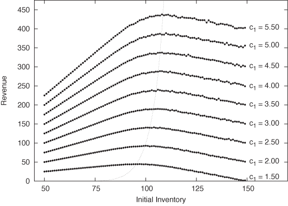
This problem lends itself nicely to simulations. The listing that follows shows a minimal program for simulating the newsvendor problem. We fix the purchase price c0 at $1 and read the projected sales price c1 from the command line. For the demand, we assume a Gaussian distribution with mean μ = 100 and standard deviation σ = 10. Now, for each possible initial level of inventory n, we make 1,000 random trials. Each trial corresponds to a single “day”; we randomly generate a level of demand m and calculate the resulting revenue for that day. The revenue consists of the sales price for the number of units that were actually sold less the purchase price for the inventory. You should convince yourself that the number of units sold is the lesser of the inventory and the demand: in the first case, we sold out; in the second case, we ended up discarding inventory. Finally, we average all trials for the current level of starting inventory and print the average revenue generated. The results are shown in Figure 17-2 for several different sales prices c1:
from sys import argv
from random import gauss

c0, c1 = 1.0, float( argv[1] )
mu, sigma = 100, 10
maxtrials = 1000

for n in range( mu-5*sigma, mu+5*sigma ):
    avg = 0
    for trial in range( maxtrials ):
        m = int( 0.5 + gauss( mu, sigma ) )
        r = c1*min( n, m ) -  c0*n
        avg += r

    print c1, n, avg/maxtrials
Of course, the total revenue depends on the actual sales price—the higher the price, the more we take home. But we can also see that, for each value of the sales price, the revenue curve has a maximum at a different horizontal location. The corresponding value of n gives us the optimal initial inventory level for that sales price. Thus we have achieved our objective: we have found the optimal number of newspapers to buy at the beginning of the day to maximize our earnings.
This simple idea can be extended in different ways. More complicated situations may involve different types of items, each with its own demand distribution. How much of each item should we hold in inventory now? Alternatively, we can turn the problem around by asking: given a fixed inventory, what would be the optimal price to maximize earnings? To answer this question, we need to know how the demand varies as we change the price—that is, we need to know the demand curve, which takes the role of the demand distribution in our example.
Optional: Exact Solution
For this particular example, involving only a single type of product at a fixed price, we can actually work out the optimum exactly. (This means that running a simulation wasn’t strictly necessary in this case. Nevertheless, this is one of those cases where a simulation may actually be easier to do and less error-prone than an analytical model. For more complicated scenarios, such as those involving different types of items with different demands, simulations are unavoidable.)
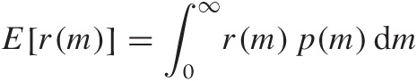
To solve this problem analytically, we want to find the optimum of the expected revenue. The revenue—as we already saw in our example simulation program—is given by
r(m) = c1 min(n, m) – c0n
The revenue depends on the demand m. However, the demand is a random quantity: all that we know is that it is distributed according to some distribution p(m). The expected revenue E[r(m)] is the average of the revenue over all possible values of m, where each value is weighted by the appropriate probability factor:
We can now plug in the previous expression for r(m), using the lesser of n and m in the integral:
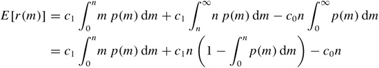
where we have made use of the fact that  and that
  .
.
We now want to find the maximum of the expected revenue with respect to the initial inventory level n. To locate the maximum, we first take the derivative with respect to n:
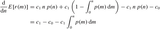
where we have used the product rule and the fundamental
theorem of calculus:  .
.
Next we equate the derivative to zero (that is the condition for the maximum) and rearrange terms to find
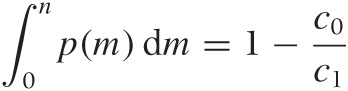
This is the final result. The lefthand side is the cumulative distribution function of the demand, and the righthand side is a simple expression involving the ratio of the purchase price and the sales price. Given the cumulative distribution function for the demand, we can now find the value of n for which the cumulative distribution function equals 1 – c0/c1—that value of n is the optimal initial inventory level.
The lighter dotted line in Figure 17-2 shows the location of the optimum revenue obtained by plugging the optimal inventory calculated in this way back into the expression for the revenue. As we would expect, this line goes right through the peaks in all the revenue curves. Notice that the maximum in the revenue curve occurs for n < 100 for c1 < 2.00: in other words, our markup has to be at least 100 percent, before it makes sense to hold more inventory than the expected average demand. (Remember that we expect to sell 100 papers on average.) If our markup is less than that, then we are better-off selling our inventory out entirely, rather than having to discard some items. (Of course, details such as these depend on the specific choice of the probability distribution p(m) that is used to model the demand.)
Further Reading
If you want to read up on some of the details that I have (quite intentionally) skipped, you should look for material on “engineering economics” or “engineering economic analysis.” Some books that I have found useful include the following.
Industrial Mathematics: Modeling in Industry, Science and Government. Charles R. MacCluer. Prentice Hall. 1999.
In his preface, MacCluer points out that most engineers leaving school “will have no experience with problems incorporating the unit $.” This observation was part of the inspiration for this chapter. MacCluer’s book contains an overview over many more advanced mathematical techniques that are relevant in practical applications. His choice of topics is excellent, but the presentation often seems a bit aloof and too terse for the uninitiated. (For instance, the material covered in this chapter is compressed into only three pages.) Available as a 2010 Dover edition under the title A Survey of Industrial Mathematics.
Schaum’s Outline of Engineering Economics. Jose Sepulveda, William Souder, and Byron Gottfried. McGraw-Hill. 1984.
If you want a quick introduction to the details left out of my presentation, then this inexpensive book is a good choice. Includes many worked examples.
Engineering Economy. William G. Sullivan, Elin M. Wicks, and C. Patrick Koelling. 14th ed., Prentice Hall. 2008.
Engineering Economic Analysis. Donald Newnan, Jerome Lavelle, and Ted Eschenbach. 10th ed., Oxford University Press. 2009.
Principles of Engineering Economic Analysis. John A. White, Kenneth E. Case, and David B. Pratt. 5th ed., Wiley. 2000.
Three standard, college-level textbooks that treat largely the same material on many more pages.
The Newsvendor Problem
Pricing and Revenue Optimization. Robert Phillips. Stanford Business Books. 2005.
Finding the optimal price for a given demand is the primary question in the field of “revenue optimization.” This book provides an accessible introduction.
Introduction to Operations Research. Frederick S. Hillier and Gerald J. Lieberman. 9th ed., McGraw-Hill. 2009.
The field of operations research encompasses a set of mathematical methods that are useful for many problems that arise in a business setting, including inventory management. This text is a standard introduction.
[28] This used to mean investing in U.S. Treasury Bonds or the equivalent, but at the time of this writing, even these are no longer considered sacrosanct. But that’s leaving the scope of this discussion!
[29] Do not confuse to depreciate, which is the process by which an asset loses value over time, with to deprecate, which is an expression of disapproval. The latter word is used most often to mark certain parts of a software program or library as deprecated, meaning that they should no longer be used in future work.