Table of Contents for
Data Analysis with Open Source Tools
 Data Analysis with Open Source Tools
Published by
O'Reilly Media, Inc., 2010
Data Analysis with Open Source Tools
Published by
O'Reilly Media, Inc., 2010
- Cover
- Data Analysis with Open Source Tools
- O'Reilly Strata Conference
- Data Analysis with Open Source Tools
- Dedication
- A Note Regarding Supplemental Files
- Preface
- 1. Introduction
- I. Graphics: Looking at Data
- 2. A Single Variable: Shape and Distribution
- 3. Two Variables: Establishing Relationships
- 4. Time As a Variable: Time-Series Analysis
- 5. More Than Two Variables: Graphical Multivariate Analysis
- 6. Intermezzo: A Data Analysis Session
- II. Analytics: Modeling Data
- 7. Guesstimation and the Back of the Envelope
- 8. Models from Scaling Arguments
- 9. Arguments from Probability Models
- 10. What You Really Need to Know About Classical Statistics
- 11. Intermezzo: Mythbusting—Bigfoot, Least Squares, and All That
- III. Computation: Mining Data
- 12. Simulations
- 13. Finding Clusters
- 14. Seeing the Forest for the Trees: Finding Important Attributes
- 15. Intermezzo: When More Is Different
- IV. Applications: Using Data
- 16. Reporting, Business Intelligence, and Dashboards
- 17. Financial Calculations and Modeling
- 18. Predictive Analytics
- 19. Epilogue: Facts Are Not Reality
- A. Programming Environments for Scientific Computation and Data Analysis
- B. Results from Calculus
- C. Working with Data
- D. About the Author
- Index
- About the Author
- Colophon
- Copyright
Chapter 7. Guesstimation and the Back of the Envelope
LOOK AROUND THE ROOM YOU ARE SITTING IN AS YOU READ THIS. NOW ANSWER THE FOLLOWING QUESTION: how many Ping-Pong balls would it take to fill this room?
Yes, I know it’s lame to make the reader do jot’em-dot’em exercises, and the question is old anyway, but please make the effort to come up with a number. I am trying to make a point here.
Done? Good—then, tell me, what is the margin of error in your result? How many balls, plus or minus, do you think the room might accommodate as well? Again, numbers, please! Look at the margin of error: can you justify it, or did you just pull some numbers out of thin air to get me off your back? And if you found an argument to base your estimate on: does the result seem right to you? Too large, too small?
Finally, can you state the assumptions you made when answering the first two questions? What did or did you not take into account? Did you take the furniture out or not? Did you look up the size of a Ping-Pong ball, or did you guess it? Did you take into account different ways to pack spheres? Which of these assumptions has the largest effect on the result? Continue on a second sheet of paper if you need more space for your answer.
The game we just played is sometimes called guesstimation and is a close relative to the back-of-the-envelope calculation. The difference is minor: the way I see it, in guesstimation we worry primarily about finding suitable input values, whereas in a typical back-of-the-envelope calculation, the inputs are reasonably well known and the challenge is to simplify the actual calculation to the point that it can be done on the back of the proverbial envelope. (Some people seem to prefer napkins to envelopes—that’s the more sociable crowd.)
Let me be clear about this: I consider proficiency at guesstimation and similar techniques the absolute hallmark of the practical data analyst—the person who goes out and solves real problems in the real world. It is so powerful because it connects a conceptual understanding (no matter how rough) with the concrete reality of the problem domain; it leaves no place to hide. Guesstimation also generates numbers (not theories or models) with their wonderful ability to cut through vague generalities and opinion-based discussions.
For all these reasons, guesstimation is a crucial skill. It is where the rubber meets the road.
The whole point of guesstimation is to come up with an approximate answer—quickly and easily. The flip side of this is that it forces us to think about the accuracy of the result: first how to estimate the accuracy and then how to communicate it. That will be the program for this chapter.
Principles of Guesstimation
Let’s step through our introductory Ping-Pong ball example together. This will give me an opportunity to point out a few techniques that are generally useful.
First consider the room. It is basically rectangular in shape. I have bookshelves along several walls; this helps me estimate the length of each wall, since I know that shelves are 90 cm (3 ft) wide—that’s a pretty universal standard. I also know that I am 1.80 m (6 ft) tall, which helps me estimate the height of the room. All told, this comes to 5 m by 3.5 m by 2.5 m or about 50 m3.
Now, the Ping-Pong ball. I haven’t had one in my hands for a long time, but I seem to remember that they are about 2.5 cm (1 in) in diameter. That means I can line up 40 of them in a meter, which means I have 403 in a cubic meter. The way I calculate this is: 403 = 43 · 103 = 26 · 1,000 = 64,000. That’s the number of Ping-Pong balls that fit into a cubic meter.
Taking things together, I can fit 50 · 64,000 or approximately 3,000,000 Ping-Pong balls into this room. That’s a large number. If each ball costs me a dollar at a sporting goods store, then the value of all the balls required to fill this room would be many times greater than the value of the entire house!
Next, the margins of error. The uncertainty in each dimension is at least 10 percent. Relative errors are added to each other in a multiplication (we will discuss error propagation later in this chapter), so the total error turns out to be 3 · 10 percent = 30 percent! That’s pretty large—the number of balls required might be as low as two million or as high as four million. It is uncomfortable to see how the rather harmless-looking 10 percent error in each individual dimension has compounded to lead to a 30 percent uncertainty.
The same problem applies to the diameter of the Ping-Pong balls. Maybe 2.5 cm is a bit low—perhaps 3 cm is more like it. Now, that’s a 20 percent increase, which means that the number of balls fitting into one cubic meter is reduced by 60 percent (3 times the relative error, again): now we can fit only about 30,000 of them into a cubic meter. The same goes for the overall estimate: a decrease by half if balls are 5 mm larger than initially assumed. Now the range is something between one and two million.
Finally, the assumptions. Yes, I took the furniture out. Given the uncertainty in the total volume of the room, the space taken up by the furniture does not matter much. I also assumed that balls would stack like cubes, when in reality they pack tighter if we arrange them in the way oranges (or cannonballs) are stacked. It’s a slightly nontrivial exercise in geometry to work out the factor, but it comes to about 15 percent more balls in the same space.
So, what can we now say with certainty? We will need a few million Ping-Pong balls—probably not less than one million and certainly not more than five million. The biggest uncertainty is the size of the balls themselves; if we need a more accurate estimate than the one we’ve obtained so far, then we can look up their exact dimensions and adjust the result accordingly.
(After I wrote this paragraph, I finally looked up the size of a regulation Ping-Pong ball: 38–40 mm. Oops. This means that only about 15,000 balls fit into a cubic meter, and so I must adjust all my estimates down by a factor of 4.)
This example demonstrates all important aspects of guesstimation:
Estimate sizes of things by comparing them to something you know.
Establish functional relationships by using simplifying assumptions.
Originally innocuous errors can compound dramatically, so tracking the accuracy of an estimate is crucial.
And finally, a few bad guesses on things that are not very familiar can have a devastating effect (I really haven’t played Ping-Pong in a long time), but they can be corrected easily when better input is available.
Still, we did find the order of magnitude, one way or the other: a few million.
Estimating Sizes
The best way to estimate the size of an object is to compare it to something you know. The shelves played this role in the previous example, although sometimes you have to work a little harder to find a familiar object to use as reference in any given situation.
Obviously, this is easier to do the more you know, and it can be very frustrating to find yourself in a situation where you don’t know anything you could use as a reference. That being said, it is usually possible to go quite far with just a few data points to use as reference values.
(There are stories from the Middle Ages of how soldiers would count how many rows of stone blocks were used in the walls of a fortress before mounting an attack, the better to estimate the height of the walls. Obtaining an accurate value was necessary to prepare scaling ladders of the appropriate length: if the ladders were too short, then the top of the wall could not be reached; if they were too long, the defenders could grab the overhanging tops and topple the ladders back over. Bottom line: you’ve got to find your reference objects where you can.)
Knowing the sizes of things is therefore the first order of business. The more you know, the easier it is to form an estimate; but also the more you know, the more you develop a feeling for the correct answer. That is an important step when operating with guesstimates: to perform an independent “sanity check” at the end to ensure we did not make some horrible mistake along the way. (In fact, the general advice is that “two (independent) estimates are better than one”; this is certainly true but not always possible—at least I can’t think of an independent way to work out the Ping-Pong ball example we started with.)
Knowing the sizes of things can be learned. All it takes is a healthy interest in the world around you—please don’t go through the dictionary, memorizing data points in alphabetical order. This is not about beating your buddies at a game of Trivial Pursuit! Instead, this is about becoming familiar (I’d almost say intimate) with the world you live in. Feynman once wrote about Hans A. Bethe that “every number was near something he knew.” That is the ideal.
The next step is to look things up. In situations where one frequently needs relatively good approximations to problems coming from a comparably small problem domain, special-purpose lookup tables can be a great help. I vividly remember a situation in a senior physics lab where we were working on an experiment (I believe, to measure the muon lifetime), when the instructor came by and asked us some guesstimation problem—I forget what it was, but it was nontrivial. None of us had a clue, so he whipped out from his back pocket a small booklet the size of a playing card that listed the physical properties of all kinds of subnuclear particles. For almost any situation that could arise in the lab, he had an approximate answer right there.
Specialized lookup tables exist in all kinds of disciplines, and you might want to make your own as necessary for whatever it is you are working on. The funniest I have seen gave typical sizes (and costs) for all elements of a manufacturing plant or warehouse: so many square feet for the office of the general manager, so many square feet for his assistant (half the size of the boss’s), down to the number of square feet per toilet stall, and—not to forget—how many toilets to budget for every 20 workers per 8-hour shift.
Finally, if we don’t know anything close and we can’t look anything up, then we can try to estimate “from the ground up”: starting just with what we know and then piling up arguments to arrive at an estimate. The problem with this approach is that the result may be way off. We have seen earlier how errors compound, and the more steps we have in our line of arguments the larger the final error is likely to be—possibly becoming so large that the result will be useless. If that’s the case, we can still try and find a cleverer argument that makes do with fewer argument steps. But I have to acknowledge that occasionally we will find ourselves simply stuck: unable to make an adequate estimate with the information we have.
The trick is to make sure this happens only rarely.
Establishing Relationships
Establishing relationships that get us from what we know to what we want to find is usually not that hard. This is true in particular under common business scenarios, where the questions often revolve around rather simple relationships (how something fits into something else, how many items of a kind there are, and the like). In scientific applications, this type of argument can be harder. But for most situations that we are likely to encounter outside the science lab, simple geometric and counting arguments will suffice.
In the next chapter, we will discuss in more detail the kinds of arguments you can use to establish relationships. For now, just one recommendation: make it simple! Not: keep it simple because, more likely than not, initially the problem is not simple; hence you have to make it so in order to make it tractable.
Simplifying assumptions let you cut through the fog and get to the essentials of a situation. You may incur an error as you simplify the problem, and you will want to estimate its effect, but at least you are moving toward a result.
An anecdote illustrates what I mean. When working for Amazon.com, I had a discussion with a rather sophisticated mathematician about how many packages Amazon can typically fit onto a tractor-trailer truck, and he started to work out the different ways you can stack rectangular boxes into the back of the truck! This is entirely missing the point because, for a rough calculation, we can make the simplifying assumption that the packages can take any shape at all (i.e., they behave like a liquid) and simply divide the total volume of the truck by the typical volume of a package. Since the individual package is tiny compared to the size of the truck, the specific shapes and arrangements of individual packages are irrelevant: their effect is much smaller than the errors in our estimates for the size of the truck, for instance. (We’ll discuss this in more detail in Chapter 8, where we discuss the mean-field approximation.)
The point of back-of-the-envelope estimates is to retain only the core of the problem, stripping away as much nonessential detail as possible. Be careful that your sophistication does not get in the way of finding simple answers.
Working with Numbers
When working with numbers, don’t automatically reach for a calculator! I know that I am now running the risk of sounding ridiculous—praising the virtues of old-fashioned reading, ‘riting, and ‘rithmetic. But that’s not my point. My point is that it is all right to work with numbers. There is no reason to avoid them.
I have seen the following scenario occur countless times: a discussion is under way, everyone is involved, ideas are flying, concentration is intense—when all of a sudden we need a few numbers to proceed. Immediately, everything comes to a screeching halt while several people grope for their calculators and others fire up their computers, followed by hasty attempts to get the required answer, which invariably (given the haste) leads to numerous keying errors and false starts, followed by arguments about the best calculator software to use. In any case, the whole creative process just died. It’s a shame.
Besides forcing you to switch context, calculators remove you one step further from the nature of the problem. When working out a problem in your head, you get a feeling for the significant digits in the result: for which digits does the result change as the inputs take on any value from their permissible range? The surest sign that somebody has no clue is when they quote the results from a calculation based on order-of-magnitude inputs to 16 digits!
The whole point here is not to be religious about it—either way. If it actually becomes more complicated to work out a numerical approximation in your head, then by all means use a calculator. But the compulsive habit to avoid working with numbers at all cost should be restrained.
There are a few good techniques that help with the kinds of calculations required for back-of-the-envelope estimates and that are simple enough that they still (even today) hold their own against uncritical calculator use. Only the first is a must-have; the other two are optional.
Powers of ten
The most important technique for deriving order-of-magnitude estimates is to work with orders of magnitudes directly—that is, with powers of ten.
It quickly gets confusing to multiply 9,000 by 17 and then to divide by 400, and so on. Instead of trying to work with the numbers directly, split each number into the most significant digit (or digits) and the respective power of ten. The multiplications now take place among the digits only while the powers of ten are summed up separately. In the example I just gave, we split 9,000 = 9 · 1,000, 17 = 1.7 · 10 ≈ 2 · 10, and 400 = 4 · 100. From the leading digits we have 9 times 2 divided by 4 equals 4.5, and from the powers of ten we have 3 plus 1 minus 2 equals 2; so then 4.5 · 102 = 450. That wasn’t so hard, was it? (I have replaced 17 with 2 · 10 in this approximation, so the result is a bit on the high side, by about 15 percent. I might want to correct for that in the end—a better approximation would be closer to 390. The exact value is 382.5.)
More systematically, any number can be split into a decimal fraction and a power of ten. It will be most convenient to require the fraction to have exactly one digit before the decimal point, like so:
123.45 = 1.2345 · 102
1,000,000 = 1.0 · 106
0.00321 = 3.21 · 10–3
The fraction is commonly known as the mantissa (or the significand in most recent usage), whereas the power of ten is always referred to as the exponent.
This notation significantly simplifies multiplication and division between numbers of very different magnitude: the mantissas multiply (involving only single-digit multiplications, if we restrict ourselves to the most significant digit), and the exponents add. The biggest challenge is to keep the two different tallies simultaneously in one’s head.
Small perturbations
The techniques in this section are part of a much larger family of methods known as perturbation theory, methods that play a huge role in applied mathematics and related fields. The idea is always the same—we split the original problem into two parts: one that is easy to solve and one that is somehow “small” compared to the first. If we do it right, the effect of the latter part is only a “small perturbation” to the first, easy part of the problem. (You may want to review Appendix B if some of this material is unfamiliar to you.)
The easiest application of this idea is in the calculation of simple powers, such as 123. Here is how we would proceed:
123 = (10 + 2)3 | = 103 + 3 · 102 · 2 + 3 · 10 · 22 + 23 |
= 1,000 + 600 + ··· | |
= 1,600 + ··· |
In the first step, we split 12 into 10 + 2: here 10 is the easy part (because we know how to raise 10 to an integer power) and 2 is the perturbation (because 2 ≪ 10). In the next step, we make use of the binomial formula (see Appendix B), ignoring everything except the linear term in the “perturbation.” The final result is pretty close to the exact value.
The same principle can be applied to many other situations. In the context of this chapter, I am interested in this concept because it gives us a way to estimate and correct for the error introduced by ignoring all but the first digit in powers-of-ten calculations. Let’s look at another example:
32 · 430
Using only the most significant digits, this is (3 · 101) · (4 · 102) = (3 · 4) · 101+2 = 12,000. But this is clearly not correct, because we dropped some digits from the factors.
We can consider the nonleading digits as small perturbations to the result and treat them separately. In other words, the calculation becomes:
(3 + 0.2) · (4 + 0.3) · 103 ≈ 3(1 + 0.1 ...) · 4(1 + 0.1 ...) · 103
where I have factored out the largest factor in each term. On the righthand side I did not write out the correction terms in full—for our purposes, it’s enough to know that they are about 0.1.
Now we can make use of the binomial formula:
(1 + ϵ)2 = 1 + 2ϵ + ϵ2
We drop the last term (since it will be very small compared to the other two), but the second term gives us the size of the correction: +2ϵ. In our case, this amounts to about 20 percent, since ϵ is one tenth.
I will admit that this technique seems somewhat out of place today, although I do use it for real calculations when I don’t have a calculator on me. But the true value of this method is that it enables me to estimate and reason about the effect that changes to my input variables will have on the overall outcome. In other words, this method is a first step toward sensitivity analysis.
Logarithms
This is the method by which generations before us performed numerical calculations. The crucial insight is that we can use logarithms for products (and exponentiation) by making use of the functional equation for logarithms:
log(xy) = log(x) + log(y)
In other words, instead of multiplying two numbers, we can add their logarithms. The slide rule was a mechanical calculator based on this idea.
Amazingly, using logarithms for multiplication is still relevant—but in a slightly different context. For many statistical applications (in particular when using Bayesian methods), we need to multiply the probabilities of individual events in order to arrive at the probability for the combination of these events. Since probabilities are by construction less than 1, the product of any two probabilities is always smaller than the individual factors. It does not take many probability factors to underflow the floating-point precision of almost any standard computer. Logarithms to the rescue! Instead of multiplying the probabilities, take logarithms of the individual probabilities and then add the logarithms. (The logarithm of a number that is less than 1 is negative, so one usually works with –log(p).) The resulting numbers, although mathematically equivalent, have much better numerical properties. Finally, since in many applications we mostly care which of a selection of different events has the maximum probability, we don’t even need to convert back to probabilities: the event with maximum probability will also be the one with the maximum (negative) logarithm.
More Examples
We have all seen this scene in many a Hollywood movie: the gangster comes in to pay off the hitman (or pay for the drug deal, or whatever it is). Invariably, he hands over an elegant briefcase with the money—cash, obviously. Question: how much is in the case?
Well, a briefcase is usually sized to hold two letter-size papers next to each other; hence it is about 17 by 11 inches wide, and maybe 3 inches tall (or 40 by 30 by 7 centimeters). A bank note is about 6 inches wide and 3 inches tall, which means that we can fit about six per sheet of paper. Finally, a 500-page ream of printer paper is about 2 inches thick. All told, we end up with 2 · 6 · 750 = 9,000 banknotes. The highest dollar denomination in general circulation is the $100 bill,[14] so the maximum value of that payoff was about $1 million, and certainly not more than $5 million.
Conclusion: for the really big jobs, you need to pay by check. Or use direct transfer.
For a completely different example, consider the following question. What’s the typical takeoff weight of a large, intercontinental jet airplane? It turns out that you can come up with an approximate answer even if you don’t know anything about planes.
A plane is basically an aluminum tube with wings. Ignore the wings for now; let’s concentrate on the tube. How big is it? One way to find out is to check your boarding pass: it will display your row number. Unless you are much classier than your author, chances are that it shows a row number in the range of 40–50. You can estimate that the distance between seats is a bit over 50 cm—although it feels closer. (When you stand in the aisle, facing sideways, you can place both hands comfortably on the tops of two consecutive seats; your shoulders are about 30 cm apart, so the distance between seats must be a tad greater than that.) Thus we have the length: 50 · 0.5 m. We double this to make up for first and business class, and to account for cockpit and tail. Therefore, the length of the tube is about 50 m. How about its diameter? Back in economy, rows are about 9 seats abreast, plus two aisles. Each seat being just a bit wider than your shoulders (hopefully), we end up with a diameter of about 5 m. Hence we are dealing with a tube that is 50 m long and 5 m in diameter.
As you walked through the door, you might have noticed the strength or thickness of the tube: it’s about 5 mm. Let’s make that 10 mm (1 cm) to account for “stuff”: wiring, seats, and all kinds of other hardware that’s in the plane. Imagining now that you unroll the entire plane (the way you unroll aluminum foil), the result is a sheet that is 50 · π · 5 · 0.01m3. The density of aluminum is a little higher than water (if you have ever been to a country that uses aluminum coins, you know that you can barely make them float), so let’s say it’s 3 g/cm3.
Length | Width | Diameter | Weight (empty) | Weight (full) | Passengers | |
B767 | 50 m | 50 m | 5 m | 90 t | 150 t | 200 |
B747 | 70 m | 60 m | 6.5 m | 175 t | 350 t | 400 |
A380 | 75 m | 80 m | 7 m | 275 t | 550 t | 500 |
It is at this point that we need to employ the proverbial back of the envelope (or the cocktail napkin they gave you with the peanuts) to work out the numbers. It will help to realize that there are 1003 = 106 cubic centimeters in a cubic meter and that the density of aluminum can therefore be written as 3 tons per cubic meter. The final mass of the “tube” comes out to about 25 ton. Let’s double this to take into account the wings (wings are about as long as the fuselage is wide—if you look at the silhouette of a plane in the sky, it forms an approximate square); this yields 50 ton just for the “shell” of the airplane. It does not take into account the engines and most of the other equipment inside the plane.
Now let’s compare this number with the load. We have 50 rows, half of them with 9 passengers and the other half with 5; this gives us an average of 7 passengers per row or a total of 350 passengers per plane. Assuming that each passenger contributes 100 kg (body weight and baggage), the load amounts to 35 ton: comparable to the weight of the plane itself. (This weight-to-load ratio is actually not that different than for a car, fully occupied by four people. Of course, if you are driving alone, then the ratio for the car is much worse.)
How well are we doing? Actually, not bad at all: Table 7-1 lists typical values for three planes that are common on transatlantic routes: the mid size Boeing 767, the large Boeing 747 (the “Jumbo”), and the extra-large Airbus 380. That’s enough to check our calculations. We are not far off.
(What we totally missed is that planes don’t fly on air and in-flight peanuts alone: in fact, the greatest single contribution to the weight of a fully loaded and fuelled airplane is the weight of the fuel. You can estimate its weight as well, but to do so, you will need one additional bit of information: the fuel consumption of a modern jet airplane per passenger and mile traveled is less than that of a typical compact car with only a single passenger.)
That was a long and involved estimation, and I won’t blame you if you skipped some of the intermediate steps. In case you are just joining us again, I’d like to emphasize one point: we came up with a reasonable estimate without having to resort to any “seat of the pants” estimates—even though we had no prior knowledge! Everything that we used, we could either observe directly (such as the number of rows in the plane or the thickness of the fuselage walls) or could relate to something that was familiar to us (such as the distance between seats). That’s an important takeaway!
But not all calculations have to be complicated. Sometimes, all you have to do is “put two and two together.” A friend told me recently that his company had to cut their budget by a million dollars. We knew that the overall budget for this company was about five million dollars annually. I also knew that, since it was mostly a service company, almost all of its budget went to payroll (there was no inventory or rent to speak of). I could therefore tell my friend that layoffs were around the corner—even with a salary reduction program, the company would have to cut at least 15 percent of their staff. The response was: “Oh, no, our management would never do that.” Two weeks later, the company eliminated one third of all positions.
Things I Know
Table 7-2 is a collection of things that I know and frequently use to make estimates. Of course, this list may seem a bit whimsical, but it is actually pretty serious. For instance, note the range of areas from which these items are drawn! What domains can you reason about, given the information in this table?
Also notice the absence of systematic “scales.” That is no accident. I don’t need to memorize the weights of a mouse, a cat, and a horse—because I know (or can guess) that a mouse is 1,000 times smaller than a human, a cat 10 times smaller, and a horse 10 times larger. The items in this table are not intended to be comprehensive; in fact, they are the bare minimum. Knowing how things relate to each other lets me take it from there.
Of course, this table reflects my personal history and interests. Yours will be different.
How Good Are Those Numbers?
Remember the Ping-Pong ball question that started out this chapter? I once posted that question as a homework problem in a class, and one student’s answer was something like 1,020,408.16327. (Did you catch both mistakes? Not only does the result of this rough estimate pretend to be accurate to within a single ball; but the answer also includes a fractional part—which is meaningless, given the context.) This type of confusion is incredibly common: we focus so much on the calculation (any calculation) that we forget to interpret the result!
This story serves as a reminder that there are two questions that we should ask before any calculation as well as one afterward. The two questions to ask before we begin are:
What level of correctness do I need?
What level of correctness can I afford?
Size of an atomic data type | 10 bytes |
A page of text | 55 lines of 80 characters, or about 4,500 characters total |
A record (of anything) | 100–1,000 bytes |
A car | 4 m long, 1 ton weight |
A person | 2 m tall, 100 kg weight |
A shelf | 1 m wide, 2 m tall |
Swimming pool (not Olympic) | 25 × 12.5 meters |
A story in a commercial building | 4 m high |
Passengers on a large airplane | 350 |
Speed of a jetliner | 1,000 km/hr |
Flight time from NY | 6 hr (to the West Coast or Europe) |
Human, walking | 1 m/s (5 km/hr) |
Human, maximum power output | 200 W (not sustainable) |
Power consumption of a water kettle | 2 kW |
Electricity grid | 100 V (U.S.), 220 V (Europe) |
Household fuse | 16 A |
3 · 3 | 10 (minus 10%) |
π | 3 |
Large city | 1 million |
Population, Germany or Japan | 100 million |
Population, USA | 300 million |
Population, China or India | 1 billion |
Population, Earth | 7 billion |
U.S. median annual income | $60,000 |
U.S. federal income tax rate | 25% (but also as low as 0% and as high as 40%) |
Minimum hourly wage | $10 per hour |
Billable hours in a year | 2,000 (50 weeks at 40 hours per week) |
Low annual inflation | 2% |
High annual inflation | 8% |
Price of a B-2 bomber | $2 billion |
American Civil War; Franco-Prussian War | 1860s; 1870s |
French Revolution | 1789 |
Reformation | 1517 |
Charlemagne | 800 |
Great Pyramids | 3000 B.C.E. |
Hot day | 35 Celsius |
Very hot kitchen oven | 250 Celsius |
Steel melts | 1200 Celsius |
Density of water | 1 g/cm3 |
Density of aluminum | 3 g/cm3 |
Density of lead | 13 g/cm3 |
Density of gold | 20 g/cm3 |
Ionization energy of hydrogen | 13.6 eV |
Atomic diameter (Bohr radius) | 10–10 m |
Energy of X-ray radiation | keV |
Nuclear binding energy per particle | MeV |
Wavelength of the sodium doublet | 590 nm |
The question to ask afterward is:
What level of correctness did I achieve?
I use the term “correctness” here a bit loosely to refer to the quality of the result. There are actually two different concepts involved: accuracy and precision.
Accuracy
Accuracy expresses how close the result of a calculation or measurement comes to the “true” value. Low accuracy is due to systematic error.
Precision
Precision refers to the “margin of error” in the calculation or the experiment. In experimental situations, precision tells us how far the results will stray when the experiment is repeated several times. Low precision is due to random noise.
Said another way: accuracy is a measure for the correctness of the result, and precision is a measure of the result’s uncertainty.
Before You Get Started: Feasibility and Cost
The first question (what level of correctness is needed) will define the overall approach—if I only need an order-of-magnitude approximation, then the proverbial back of the envelope will do; if I need better results, I might need to work harder. The second question is the necessary corollary: it asks whether I will be able to achieve my goal given the available resources. In other words, these two questions pose a classic engineering trade-off (i.e., they require a regular cost–benefit analysis).
This obviously does not matter much for a throwaway calculation, but it matters a lot for bigger projects. I once witnessed a huge project (involving a dozen developers for over a year) to build a computation engine that had failed to come clear on both counts until it was too late. The project was eventually canceled when it turned out that it would cost more to achieve the accuracy required than the project was supposed to gain the company in increased revenue! (Don’t laugh—it could happen to you. Or at least in your company.)
This story points to an important fact: correctness is usually expensive, and high correctness is often disproportionally more expensive. In other words, a 20 percent approximation can be done on the back of an envelope, a 5 percent solution can be done in a couple of months, but the cost for a 1 percent solution may be astronomical. It is also not uncommon that there is no middle ground (e.g., an affordable 10 percent solution).
I have also seen the opposite problem: projects chasing correctness that is not really necessary—or not achievable because the required input data is not available or of poor quality. This is a particular risk if the project involves the opportunity to play with some attractive new technology.
Finding out the true cost or benefit of higher-quality results can often be tricky. I was working on a project to forecast the daily number of visitors viewing the company’s website, when I was told that “we must have absolute forecast accuracy; nothing else matters.” I suggested that if this were so, then we should take the entire site down, since doing so would guarantee a perfect forecast (zero page views). Yet because this would also imply zero revenue from display advertising, my suggestion focused the client’s mind wonderfully to define more clearly what “else” mattered.
After You Finish: Quoting and Displaying Numbers
It is obviously pointless to report or quote results to more digits than is warranted. In fact, it is misleading or at the very least unhelpful, because it fails to communicate to the reader another important aspect of the result—namely its reliability!
A good rule (sometimes known as Ehrenberg’s rule) is to quote all digits up to and including the first two variable digits. Starting from the left, you keep all digits that do not change over the entire range of numbers from one data point to the next; then you also keep the first two digits that vary over the entire range from 0 to 9 as you scan over all data points. An example will make this clear. Consider the following data set:
121.733
122.129
121.492
119.782
120.890
123.129
Here, the first digit (from the left) is always 1 and the second digit takes on only two values (1 and 2), so we retain them both. All further digits can take on any value between 0 and 9, and we retain the first two of them—meaning that we retain a total of four digits from the left. The two right-most digits therefore carry no significance, and we can drop them when quoting results. The mean (for instance) should be reported as:
121.5
Displaying further digits is of no value.
This rule—to retain the first two digits that vary over the entire range of values and all digits to the left of them—works well with the methods described in this chapter. If you are working with numbers as I suggested earlier, then you also develop a sense for the digits that are largely unaffected by reasonable variations in the input parameters as well as for the position in the result after which uncertainties in the input parameters corrupt the outcome.
Finally, a word of warning. The accuracy level of a numerical result should be established from the outset, since doing so later will trigger resistance. I have encountered a system that reported projected sales numbers (which were typically in the hundreds of thousands) to six “significant” digits (e.g., as 324,592 or so). But because these were forecasts that were at best accurate to within 30 percent, all digits beyond the first were absolute junk! (Note that 30 percent of 300,000 is 100,000, which means that the confidence band for this result was 200,000–400,000.) However, a later release of the same software, which now reported only the actually significant digits, was met by violent opposition from the user community because it was “so much less precise”!
Optional: A Closer Look at Perturbation Theory and Error Propagation
I already mentioned the notion of “small perturbations.” It is one of the great ideas of applied mathematics, so it is worth a closer look.
Whenever we can split a problem into an “easy” part and a part that is “small,” the problem lends itself to a perturbative solution. The “easy” part we can solve directly (that’s what we mean by “easy”), and the part that is “small” we solve in an approximative fashion. By far the most common source of approximations in this area is based on the observation that every function (every curve) is linear (a straight line) in a sufficiently small neighborhood: we can therefore replace the full problem by its linear approximation when dealing with the “small” part—and linear problems are always solvable.
As a simple example, let’s calculate  . Can we split this into a “simple” and a
“small” problem? Well, we know that 16 = 42
and so
. Can we split this into a “simple” and a
“small” problem? Well, we know that 16 = 42
and so  . That’s the simple part, and we therefore now
write
. That’s the simple part, and we therefore now
write  . Obviously 1 ≪ 16, so there’s the “small” part
of the problem. We can now rewrite our problem as follows:
. Obviously 1 ≪ 16, so there’s the “small” part
of the problem. We can now rewrite our problem as follows:
It is often convenient to factor out everything so that we are left with 1 + small stuff as in the second line here. At this point, we also replaced the small part with ϵ (we will put the numeric value back in at the end).
So far everything has been exact, but to make progress we need
to make an approximation. In this case, we replace the square root by
a local approximation around 1. (Remember: ϵ is small, and
 is easy.) Every smooth function can be replaced
by a straight line locally, and if we don’t go too far, then that
approximation turns out to be quite good (see Figure 7-1). These
approximations can be derived in a systematic fashion by a process
known as Taylor expansion. The figure shows both
the simplest approximation, which is just a straight line, and also
the next-higher (second-order) approximation, which is even
better.
is easy.) Every smooth function can be replaced
by a straight line locally, and if we don’t go too far, then that
approximation turns out to be quite good (see Figure 7-1). These
approximations can be derived in a systematic fashion by a process
known as Taylor expansion. The figure shows both
the simplest approximation, which is just a straight line, and also
the next-higher (second-order) approximation, which is even
better.
Taylor expansions are so fundamental that they are almost considered a fifth basic operation (after addition, subtraction, multiplication, and division). See Appendix B for a little more information on them.

With the linear approximation in place, our problem has now become quite tractable:
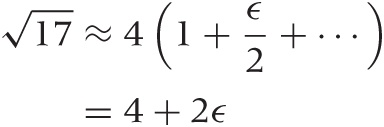
We can now plug the numeric value ϵ = 1/16 back in:
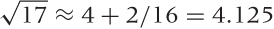 . The exact value is
  .... Our approximation is pretty good.
Error Propagation
Error propagation considers situations where we have some quantity x and an associated uncertainty δx. We write x ± δx to indicate that we expect the true value to lie anywhere in the range from x – δx to x + δx. In other words, we have not just a single value for the quantity x, but instead a whole range of possible values.
Now suppose we have several quantities—each with its own error term—and we need to combine them in some fashion. We probably know how to work with the quantities themselves, but what about the uncertainties? For example, we know both the height and width of a rectangle to within some range: h + δh and w + δw. We also know that the area is A = hw (from basic geometry). But what can we say about the uncertainty in the area?
This kind of scenario is ideal for the perturbative methods discussed earlier: the uncertainties are “small,” so we can use simplifying approximations to deduce their behavior.
Let’s work through the area example:
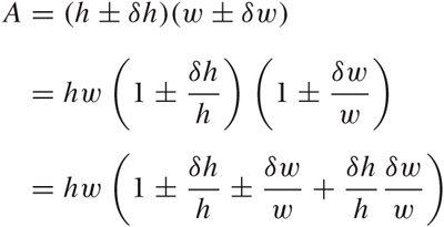
Here again we have factored the primary terms out, to end up with terms of the form 1 + small stuff, because that makes life easier. This also means that, instead of expressing the uncertainty through the absolute error δh or δw, we express them through the relative error δh/h or δw/w. (Observe that if δh ≪ h, then δh/h ≪ 1.)
So far, everything has been exact. Now comes the
approximation: the error terms are small (in fact, smaller than 1);
hence their product is extra-small, and we can therefore drop it.
Our final result is thus  or, in words: “When multiplying two
quantities, their relative errors add.” So if I know both the width
and the height to within 10 percent each, then my uncertainty in the
area will be 20 percent.
or, in words: “When multiplying two
quantities, their relative errors add.” So if I know both the width
and the height to within 10 percent each, then my uncertainty in the
area will be 20 percent.
Here are a few more results of this form, which are useful whenever you work with quantities that have associated uncertainties (you might want to try deriving some of these yourself):
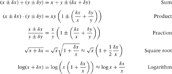
The most important ones are the first two: when adding (or subtracting) two quantities, their absolute errors add; and when multiplying (or dividing) two quantities, their relative errors add. This implies that, if one of two quantities has a significantly larger error than the other, then the larger error dominates the final uncertainty.
Finally, you may have seen a different way to calculate errors that gives slightly tighter bounds, but it is only appropriate if the errors have been determined by calculating the variances in repeated measurements of the same quantity. Only in that case are the statistical assumptions valid upon which this alternative calculation is based. For guesstimation, the simple (albeit more pessimistic) approach described here is more appropriate.
Workshop: The Gnu Scientific Library (GSL)
What do you do when a calculation becomes too involved to do it in your head or even on the back of an envelope? In particular, what can you do if you need the extra precision that a simple order-of-magnitude estimation (as practiced in this chapter) will not provide? Obviously, you reach for a numerical library!
The Gnu Scientific Library, or GSL, (http://www.gnu.org/software/gsl/) is the best currently available open source library for numerical and scientific calculations that I am aware of. The list of included features is comprehensive, and the implementations are of high quality. Thanks to some unifying conventions, the API, though forbidding at first, is actually quite easy to learn and comfortable to use. Most importantly, the library is mature, well documented, and reliable.
Let’s use it to solve two rather different problems; this will give us an opportunity to highlight some of the design choices incorporated into the GSL. The first example involves matrix and vector handling: we will calculate the singular value decomposition (SVD) of a matrix. The second example will demonstrate how the GSL handles non-linear, iterative problems in numerical analysis as we find the minimum of a nonlinear function.
The listing that follows should give you a flavor of what vector and matrix operations look like when using the GSL. First, we allocate a couple of (two-dimensional) vectors and assign values to their elements. We then perform some basic vector operations: adding one vector to another and performing a dot product. (The result of a dot product is a scalar, not another vector.) Finally, we allocate and initialize a matrix and calculate its SVD. (See Chapter 14 for more information on vector and matrix operations.)
/* Basic Linear Algebra using the GSL */

#include <stdio.h>
#include <gsl/gsl_vector.h>
#include <gsl/gsl_matrix.h>
#include <gsl/gsl_blas.h>
#include <gsl/gsl_linalg.h>

int main()  {
  double r;

  gsl_vector *a, *b, *s, *t;
  gsl_matrix *m, *v;


  /* --- Vectors --- */
  a = gsl_vector_alloc( 2 );    /* two dimensions */
  b = gsl_vector_alloc( 2 );

  /* a = [ 1.0, 2.0 ] */
  gsl_vector_set( a, 0, 1.0 );
  gsl_vector_set( a, 1, 2.0 );
  /* b = [ 3.0, 6.0 ] */
  gsl_vector_set( b, 0, 3.0 );
  gsl_vector_set( b, 1, 6.0 );

  /* a += b (so that now  a = [ 4.0, 8.0 ]) */
  gsl_vector_add( a, b );
  gsl_vector_fprintf( stdout, a, "%f" );

  /* r = a . b  (dot product) */
  gsl_blas_ddot( a, b, &r );
  fprintf( stdout, "%f\n", r );

  /* --- Matrices --- */
  s = gsl_vector_alloc( 2 );
  t = gsl_vector_alloc( 2 );

  m = gsl_matrix_alloc( 2, 2 );
  v = gsl_matrix_alloc( 2, 2 );

  /* m = [ [1, 2],
           [0, 3] ] */
  gsl_matrix_set( m, 0, 0, 1.0 );
  gsl_matrix_set( m, 0, 1, 2.0 );
  gsl_matrix_set( m, 1, 0, 0.0 );
  gsl_matrix_set( m, 1, 1, 3.0 );

  /* m = U s V^T  (SVD : singular values are in vector s) */
  gsl_linalg_SV_decomp( m, v, s, t );
  gsl_vector_fprintf( stdout, s, "%f" );


  /* --- Cleanup --- */
  gsl_vector_free( a );
  gsl_vector_free( b );
  gsl_vector_free( s );
  gsl_vector_free( t );

  gsl_matrix_free( m );
  gsl_matrix_free( v );

  return 0;
}
It is becoming immediately (and a little painfully) clear that we are dealing with plain C, not C++ or any other more modern, object-oriented language! There is no operator overloading; we must use regular functions to access individual vector and matrix elements. There are no namespaces, so function names tend to be lengthy. And of course there is no garbage collection!
What is not so obvious is that element
access is actually boundary checked: if you try to access a vector
element that does not exist (e.g., gsl_vector_set( a, 4, 1.0 );), then the GSL
internal error handler will be invoked. By default, it will halt the
program and print a message to the screen. This is quite generally
true: if the library detects an error—including bad inputs, failure to
converge numerically, or an out-of-memory situation—it will invoke its
error handler to notify you. You can provide your own error handler to
respond to errors in a more flexible fashion. For a fully tested
program, you can also turn range checking on vector and matrix
elements off completely, to achieve the best
possible runtime performance.
Two more implementation details before leaving the linear
algebra example: although the matrix and vector elements are of type
double in this example, versions of
all routines exist for integer and complex data types as well.
Furthermore, the GSL will use an optimized implementation of the BLAS
(Basic Linear Algebra Subprograms) API if one is available; if not,
the GSL comes with its own, basic implementation.
Now let’s take a look at the second example. Here we use the GSL to find the minimum of a one-dimensional function. The function to minimize is defined at the top of the listing: x2 log(x). In general, nonlinear problems such as this must be solved iteratively: we start with a guess, then calculate a new trial solution based on that guess, and so on until the result meets whatever stopping criteria we care to define.
At least that’s what the introductory textbooks tell you.
In the main part of the program, we instantiate a “minimizer,” which is an encapsulation of a specific minimization algorithm (in this case, Golden Section Search—others are available, too) and initialize it with the function to minimize as well as our initial guess for the interval containing the minimum.
Now comes the surprising part: an explicit loop! In this loop, the “minimizer” takes a single step in the iteration (i.e., calculates a new, tighter interval bounding the minimum) but then essentially hands control back to us. Why so complicated? Why can’t we just specify the desired accuracy of the interval and let the library handle the entire iteration for us? The reason is that real problems more often than not don’t converge as obediently as the textbooks suggest! Instead they can (and do) fail in a variety of ways: they converge to the wrong solution, they attempt to access values for which the function is not defined, they attempt to make steps that (for reasons of the larger system of which the routine is only a small part) are either too large or too small, or they diverge entirely. Based on my experience, I have come to the conclusion that every nonlinear problem is different (whereas every linear problem is the same), and therefore generic black-box routines don’t work!
This brings us back to the way this minimization routine is implemented: the required iteration is not a black box and instead is open and accessible to us. We can simply monitor its progress (as we do in this example, by printing every iteration step to the screen), but we could also interfere with it—for instance to enforce some invariant that is specific to our problem. The “minimizer” does as much as it can by calculating and proposing a new interval; ultimately, however, we are in control over how the iteration progresses. (For the textbook example used here, this doesn’t matter, but it makes all the difference when you are doing serious numerical analysis on real problems!)
/* Minimizing a function with the GSL */

#include <stdio.h>
#include <gsl/gsl_min.h>

double fct( double x, void *params )  {
  return x*x*log(x);
}

int main()  {
  double a = 0.1, b = 1; /*  interval which bounds the minimum */

  gsl_function f;        /* pointer to the function to minimize */
  gsl_min_fminimizer *s; /* pointer to the minimizer instance */

  f.function = &fct;     /* the function to minimize */
  f.params = NULL;       /* no additional parameters needed */

  /* allocate the minimizer, choosing a particular algorithm */
  s = gsl_min_fminimizer_alloc( gsl_min_fminimizer_goldensection );

  /* initialize the minimizer with a function an an initial interval */
  gsl_min_fminimizer_set( s, &f, (a+b)/2.0, a, b );

  while ( b-a > 1.e-6 )  {
    /* perform one minimization step */
    gsl_min_fminimizer_iterate( s );

    /* obtain the new bounding interval */
    a = gsl_min_fminimizer_x_lower( s );
    b = gsl_min_fminimizer_x_upper( s );

    printf( "%f\t%f\n", a, b );
  }

  printf( "Minimum Position: %f\tValue: %f\n",
          gsl_min_fminimizer_x_minimum(s), gsl_min_fminimizer_f_minimum(s) );

  gsl_min_fminimizer_free( s );

  return 0;
}
Obviously, we have only touched on the GSL. My primary intention in this section was to give you a sense for the way the GSL is designed and for what kinds of considerations it incorporates. The list of features is extensive—consult the documentation for more information.
Further Reading
Guesstimation: Solving the World’s Problems on the Back of a Cocktail Napkin. Lawrence Weinstein and John A. Adam. Princeton University Press. 2008.
This little book contains about a hundred guesstimation problems (with solutions!) from all walks of life. If you are looking for ideas to get you started, look no further.
Programming Pearls. Jon Bentley. 2nd ed., Addison-Wesley. 1999; also, More Programming Pearls: Confessions of a Coder. Jon Bentley. Addison-Wesley. 1989.
These two volumes of reprinted magazine columns are delightful to read, although (or because) they breathe the somewhat dated atmosphere of the old Bell Labs. Both volumes contain chapters on guesstimation problems in a programming context.
Back-of-the-Envelope Physics. Clifford E. Swartz. Johns Hopkins University Press. 2003.
Physicists regard themselves as the inventors of back-of-the-envelope calculations. This book contains a set of examples from introductory physics (with solutions).
The Flying Circus of Physics. Jearl Walker. 2nd ed., Wiley. 2006.
If you’d like some hints on how to take an interest in the world around you, try this book. It contains hundreds of everyday observations and challenges you to provide an explanation for each. Why are dried coffee stains always darker around the rim? Why are shower curtains pulled inward? Remarkably, many of these observations are still not fully understood! (You might also want to check out the rather different and more challenging first edition.)
Pocket Ref. Thomas J. Glover. 3rd ed., Sequoia Publishing. 2009.
This small book is an extreme example of the “lookup” model. It seems to contain almost everything: strength of wood beams, electrical wiring charts, properties of materials, planetary data, first aid, military insignia, and sizing charts for clothing. It also shows the limitations of an overcomplete collection of trivia: I simply don’t find it all that useful, but it is interesting for the breadth of topics covered.
[14] Larger denominations exist but—although legal tender—are not officially in circulation and apparently fetch far more than their face value among collectors.