Table of Contents for
Data Analysis with Open Source Tools
 Data Analysis with Open Source Tools
Published by
O'Reilly Media, Inc., 2010
Data Analysis with Open Source Tools
Published by
O'Reilly Media, Inc., 2010
- Cover
- Data Analysis with Open Source Tools
- O'Reilly Strata Conference
- Data Analysis with Open Source Tools
- Dedication
- A Note Regarding Supplemental Files
- Preface
- 1. Introduction
- I. Graphics: Looking at Data
- 2. A Single Variable: Shape and Distribution
- 3. Two Variables: Establishing Relationships
- 4. Time As a Variable: Time-Series Analysis
- 5. More Than Two Variables: Graphical Multivariate Analysis
- 6. Intermezzo: A Data Analysis Session
- II. Analytics: Modeling Data
- 7. Guesstimation and the Back of the Envelope
- 8. Models from Scaling Arguments
- 9. Arguments from Probability Models
- 10. What You Really Need to Know About Classical Statistics
- 11. Intermezzo: Mythbusting—Bigfoot, Least Squares, and All That
- III. Computation: Mining Data
- 12. Simulations
- 13. Finding Clusters
- 14. Seeing the Forest for the Trees: Finding Important Attributes
- 15. Intermezzo: When More Is Different
- IV. Applications: Using Data
- 16. Reporting, Business Intelligence, and Dashboards
- 17. Financial Calculations and Modeling
- 18. Predictive Analytics
- 19. Epilogue: Facts Are Not Reality
- A. Programming Environments for Scientific Computation and Data Analysis
- B. Results from Calculus
- C. Working with Data
- D. About the Author
- Index
- About the Author
- Colophon
- Copyright
Chapter 14. Seeing the Forest for the Trees: Finding Important Attributes
WHAT DO YOU DO WHEN YOU DON’T KNOW WHERE TO START? WHEN YOU ARE DEALING WITH A DATA SET THAT offers no structure that would suggest an angle of attack?
For example, I remember looking through a company’s contracts with its suppliers for a certain consumable. These contracts all differed in regards to the supplier, the number of units ordered, the duration of the contract and the lead time, the destination location that the items were supposed to be shipped to, the actual shipping date, and the procurement agent that had authorized the contract—and, of course, the unit price. What I tried to figure out was which of these quantities had the greatest influence on the unit price.
This kind of problem can be very difficult: there are so many different variables, none of which seems, at first glance, to be predominant. Furthermore, I have no assurance that the variables are all independent; many of them may be expressing related information. (In this case, the supplier and the shipping destination may be related, since suppliers are chosen to be near the place where the items are required.)
Because all variables arise on more or less equal footing, we can’t identify a few as the obvious “control” or independent variables and then track the behavior of all the other variables in response to these independent variables. We can try to look at all possible pairings—for example, using graphical techniques such as scatter-plot matrices (Chapter 5)—but that may not really reveal much either, particularly if the number of variables is truly large. We need some form of computational guidance.
In this chapter, we will introduce a number of different techniques for exactly this purpose. All of them help us select the most important variables or features from a multivariate data set in which all variables appear to arise on equal footing. In doing so, we reduce the dimension of the data set from the original number of variables (or features) to a smaller set, which (hopefully) captures most of the “interesting” behavior of the data. These methods are therefore also known as feature selection or dimensionality reduction techniques.
A word of warning: the material in this chapter is probably the most advanced and least obvious in the whole book, both conceptually and also with respect to actual implementations. In particular, the following section (on principal component analysis) is very abstract, and it may not make much sense if you haven’t had some previous exposure to matrices and linear algebra (including eigentheory). Other sections are more accessible.
I include these techniques here nevertheless, because they are of considerable practical importance but also to give you a sense of the kinds of (more advanced) techniques that are available, and also as a possible pointer for further study.
Principal Component Analysis
Principal component analysis (PCA) is the primary tool for dimensionality reduction in multivariate problems. It is a foundational technique that finds applications as part of many other, more advanced procedures.
Motivation
To understand what PCA can do for us, let’s consider a simple example. Let’s go back to the contract example given earlier and now assume that there are only two variables for each contract: its lead time and the number of units to be delivered. What can we say about them? Well, we can draw histograms for each to understand the distribution of values and to see whether there are “typical” values for either of these quantities. The histograms (in the form of kernel density estimates—see Chapter 2) are shown in Figure 14-1 and don’t reveal anything of interest.
Because there are only two variables in this case, we can also plot one variable against the other in a scatter plot. The resulting graph is shown in Figure 14-2 and is very revealing: the lead time of the contract grows with its size. So far, so good.
But we can also look at Figure 14-2 in a different way. Recall that the contract data depends on two variables (lead time and number of items), so that we would expect the points to fill the two-dimensional space spanned by the two axes (lead time and number of items). But in reality, all the points fall very close to a straight line. A straight line, however, is only one-dimensional, and this means that we need only a single variable to describe the position of each point: the distance along the straight line. In other words, although it appears to depend on two variables, the contract data mostly depends on a single variable that lies halfway between the original ones. In this sense, the data is of lower dimensionality than it originally appeared.
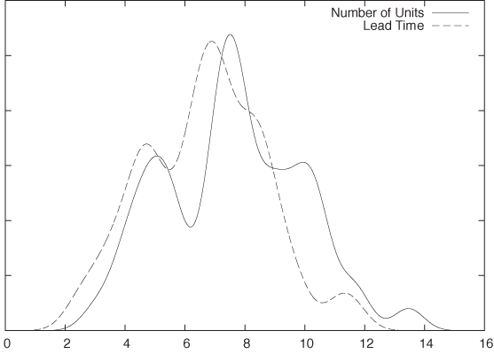
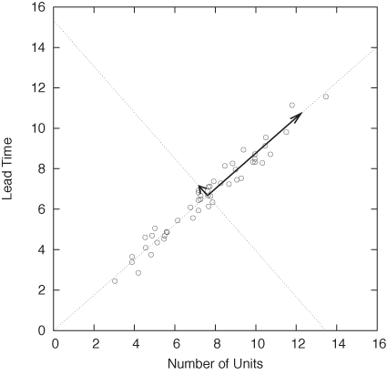
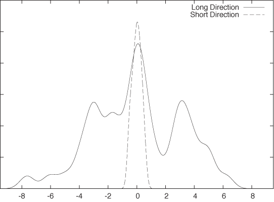
Of course, the data still depends on two variables—as it did originally. But most of the variation in the data occurs along only one direction. If we were to measure the data only along this direction, we would still capture most of what is “interesting” about the data. In Figure 14-3, we see another kernel density estimate of the same data, but this time not taken along the original variables but instead showing the distribution of data points along the two “new” directions indicated by the arrows in the scatter plot of Figure 14-2. In contrast to the variation occurring along the “long” component, the “short” component is basically irrelevant.
For this simple example, which had only two variables to begin with, it was easy enough to find the lower-dimensional representation just by looking at it. But that won’t work when there are significantly more than two variables involved. If there aren’t too many variables, then we can generate a scatter-plot matrix (see Chapter 5) containing all possible pairs of variables, but even this becomes impractical once there are more than seven or eight variables. Moreover, scatter-plot matrices can never show us more than the combination of any two of the original variables. What if the data in a three-dimensional problem falls onto a straight line that runs along the space diagonal of the original three-dimensional data cube? We will not find this by plotting the data against any (two-dimensional!) pair of the original variables.
Fortunately, there is a calculational scheme that—given a set of points—will give us the principal directions (in essence, the arrows in Figure 14-2) as a combination of the original variables. That is the topic of the next section.
Optional: Theory
We can make progress by using a technique that works for many multi-dimensional problems. If we can summarize the available information regarding the multi-dimensional system in matrix form, then we can invoke a large and powerful body of results from linear algebra to transform this matrix into a form that reveals any underlying structure (such as the structure visible in Figure 14-2).
In what follows, I will often appeal to the two-dimensional example of Figure 14-2, but the real purpose here is to develop a procedure that will be applicable to any number of dimensions. These techniques become necessary when the number of dimensions exceeds two or three so that simple visualizations like the ones discussed so far will no longer work.
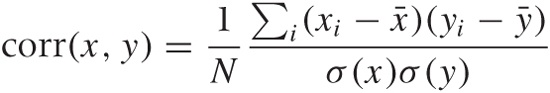
To express what we know about the system, we first need to ask ourselves how best to summarize the way any two variables relate to each other. Looking at Figure 14-2, the correlation coefficient suggests itself. In Chapter 13, we introduced the correlation coefficient as a measure for the similarity between two multi-dimensional data points x and y. Here, we use the same concept to express the similarity between two dimensions in a multivariate data set. Let x and y be two different dimensions (“variables”) in such a data set, then the correlation coefficient is defined by:
where the sum is over all data points, x̄ and ȳ are the means
of the
xi
and the
yi,
respectively, and 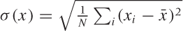 is the standard deviation of
x (and equivalently for
y). The denominator in the expression of the
correlation coefficient amounts to a rescaling of the values of both
variables to a standard interval. If that is not what we want, then
we can instead use the covariance between the
xi
and the
yi:
is the standard deviation of
x (and equivalently for
y). The denominator in the expression of the
correlation coefficient amounts to a rescaling of the values of both
variables to a standard interval. If that is not what we want, then
we can instead use the covariance between the
xi
and the
yi:
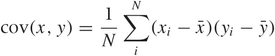
All of these quantities can be defined for any two variables (just supply values for, say xi and zi). For a p-dimensional problem, we can find all the p(p – 1)/2 different combinations (remember that these coefficients are symmetric: cov(x, y) = cov(y, x)).
It is now convenient to group the values in a matrix, which is typically called Σ (not to be confused with the summation sign!)
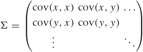
and similarly for the correlation matrix. Because the covariance (or correlation) itself is symmetric under an interchange of its arguments, the matrix Σ is also symmetric (so that it equals its transpose).
We can now invoke an extremely important result from linear algebra, known as the spectral decomposition theorem, as follows. For any real, symmetric N × N matrix A, there exists an orthogonal matrix U such that:
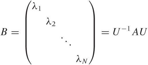
is a diagonal matrix.
Let’s explain some of the terminology. A matrix is diagonal if its only nonzero entries are along the main diagonal from the top left to the bottom right. A matrix is orthogonal if its transpose equals its inverse: UT = U–1 or UT U = UUT = 1.
The entries λi in the diagonal matrix are called the eigenvalues of matrix A, and the column vectors of U are the eigenvectors. The spectral theorem also implies that all eigenvectors are mutually orthogonal. Finally, the ith column vector in U is the eigenvector “associated” with the eigenvalue λi; each eigenvalue has an associated eigenvector.
What does all of this mean? In a nutshell, it means that we can perform a change of variables that turns any symmetric matrix A into a diagonal matrix B. Although it may not be obvious, the matrix B contains the same information as A—it’s just packaged differently.
The change of variables required for this transformation consists of a rotation of the original coordinate system into a new coordinate system in which the correlation matrix has a particularly convenient (diagonal) shape. (Notice how in Figure 14-2, the new directions are rotated with respect to the original horizontal and vertical axes.)
When expressed in the original coordinate system (i.e., the original variables that the problem was initially expressed in), the matrix Σ is a complicated object with off-diagonal entries that are nonzero. However, the eigenvectors span a new coordinate system that is rotated with respect to the old one. In this new coordinate system, the matrix takes on a simple, diagonal form in which all entries that are not on the diagonal vanish. The arrows in Figure 14-2 show the directions of the new coordinate axes, and the histogram in Figure 14-3 measures the distribution of points along these new directions.
The purpose of performing a matrix diagonalization is to find the directions of this new coordinate system, which is more suitable for describing the data than was the original coordinate system.
Because the new coordinate system is merely rotated relative
to the original one, we can express its coordinate axes as linear
combinations of the original ones. In Figure 14-2, for instance,
to make a step in the new direction (along the diagonal), you take a
step along the (old) x axis, followed by a step
along the (old) y axis. We can therefore
express the new direction (call it  ) in terms of the old ones:
 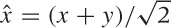 (the factor
  is just a normalization factor).
Interpretation
The spectral decomposition theorem applies to any symmetric matrix. For any such matrix, we can find a new coordinate system, in which the matrix is diagonal. But the interpretation of the results (what do the eigenvalues and eigenvectors mean?) depends on the specific application. In our case, we apply the spectral theorem to the covariance or correlation matrix of a set of points, and the results of the decomposition will give us the principal axes of the distribution of points (hence the name of the technique).
Look again at Figure 14-2. Points are distributed in a region shaped like an extremely stretched ellipse. If we calculate the eigenvalues and eigenvectors of the correlation matrix of this point distribution, we find that the eigenvectors lie in the directions of the principal axes of the ellipse while the eigenvalues give the relative length of the corresponding principal axes.
Put another way, the eigenvalues point along the directions of greatest variance: the data is most stretched out if we measure it along the principal directions. Moreover, the eigenvalue corresponding to each eigenvector is a measure of the width of the distribution along this direction.
(In fact, the eigenvalue is the square of the standard
deviation along that direction; remember that the diagonal entries
of the covariance matrix Σ are 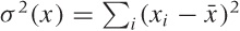 . Once we diagonalize Σ, the entries along the
diagonal—that is, the eigenvalues—are the variances along the “new”
directions.)
. Once we diagonalize Σ, the entries along the
diagonal—that is, the eigenvalues—are the variances along the “new”
directions.)
You should also observe that the variables measured along the principal directions are uncorrelated with each other. (By construction, their correlation matrix is diagonal, which means that the correlation between any two different variables is zero.)
This, then, is what the principal component analysis does for us: if the data points are distributed as a globular cloud in the space spanned by all the original variables (which may be more than two!), then the eigenvectors will give us the directions of the principal axes of the ellipsoidal cloud of data points and the eigenvalues will give us the length of the cloud along each of these directions. The eigenvectors and eigenvalues therefore describe the shape of the point distribution. This becomes especially useful if the data set has more than just two dimensions, so that a simple plot (as in Figure 14-2) is no longer feasible. (There are special varieties of PCA, such as “Kernel PCA” or “ISOMAP,” that work even with point distributions that do not form globular ellipsoids but have more complicated, contorted shapes.)
The description of the shape of the point distribution provided by the PCA is already helpful. But it gets even better, because we may suspect that not all of the original variables are really needed. Some of them may be redundant (expressing more or less the same thing), and others may be irrelevant (carrying little information).
An indication that variables may be redundant (i.e., express the “same thing”) is that they are correlated. (That’s pretty much the definition of correlation: knowing that if we change one variable, then there will be a corresponding change in the other.) The PCA uses the information contained in the mutual correlations between variables to identify those that are redundant. By construction, the principal coordinates are uncorrelated (i.e., not redundant), which means that the information contained in the original (redundant) set of variables has been concentrated in only a few of the new variables while the remaining variables have become irrelevant. The irrelevant variables are those corresponding to small eigenvalues: the point distribution will have only little spread in the corresponding directions (which means that these variables are almost constants and can therefore be ignored).
The price we have to pay for the reduction in dimensions is that the new directions will not, in general, map neatly to the original variables. Instead, the new directions will correspond to combinations of the original variables.
There is an important consequence of the preceding discussion: the principal component analysis works with the correlation between variables. If the original variables are uncorrelated, then there is no point in carrying out a PCA! For instance, if the data points in Figure 14-2 had shown no structure but had filled the entire two-dimensional parameter space randomly, then we would not have been able to simplify the problem by reducing it to a one-dimensional one consisting of the new direction along the main diagonal.
Computation
The theory just described would be of only limited interest if there weren’t practical algorithms for calculating both eigenvalues and eigenvectors. These calculations are always numerical. You may have encountered algebraic methods matrix diagonalization methods in school, but they are impractical for matrices larger than 2 × 2 and infeasible for matrices larger than about 4 × 4.
However, there are several elegant numerical algorithms to invert and diagonalize matrices, and they tend to form the foundational part of any numerical library. They are not trivial to understand, and developing high-quality implementations (that avoid, say round-off error) is a specialized skill. There are no good reasons to write your own, so you should always use an established library. (Every numerical library or package will include the required functionality.)
Matrix operations are relatively expensive, and run time
performance can be a serious concern for large matrices. Matrix
operations tend to be of  (N3)
complexity, which means that doubling the size of the matrix will
increase the time to perform an operation by a factor of 23 = 8. In
other words, doubling the problem size will result in nearly a
tenfold increase in runtime! This is not an
issue for small matrices (up to 100 × 100 or so), but you will hit a
brick wall at a certain size (somewhere between 5,000 × 5,000 and
50,000 × 50,000). Such large matrices do occur in practice but
usually not in the context of the topic of this chapter. For even
larger matrices there are alternative algorithms—which, however,
calculate only the most important of the eigenvalues and
eigenvectors.
(N3)
complexity, which means that doubling the size of the matrix will
increase the time to perform an operation by a factor of 23 = 8. In
other words, doubling the problem size will result in nearly a
tenfold increase in runtime! This is not an
issue for small matrices (up to 100 × 100 or so), but you will hit a
brick wall at a certain size (somewhere between 5,000 × 5,000 and
50,000 × 50,000). Such large matrices do occur in practice but
usually not in the context of the topic of this chapter. For even
larger matrices there are alternative algorithms—which, however,
calculate only the most important of the eigenvalues and
eigenvectors.
I will not go into details about different algorithms, but I want to mention one explicitly because it is of particular importance in this context. If you read about principal component analysis (PCA), then you will likely encounter the term singular value decomposition (SVD); in fact, many books treat PCA and SVD as equivalent expressions for the same thing. That is not correct; they are really quite different. PCA is the application of spectral methods to covariance or correlation matrices; it is a conceptual technique, not an algorithm. In contrast, the SVD is a specific algorithm that can be applied to many different problems one of which is the PCA.
The reason that the SVD features so prominently in discussions of the PCA is that the SVD combines two required steps into one. In our discussion of the PCA, we assumed that you first calculate the covariance or correlation matrix explicitly from the set of data points and then diagonalize it. The SVD performs these two steps in one fell swoop: you pass the set of data points directly to the SVD, and it calculates the eigenvalues and eigenvectors of the correlation matrix directly from those data points.
The SVD is a very interesting and versatile algorithm, which is unfortunately rarely included in introductory classes on linear algebra.
Practical Points
As you can see, principal component analysis is an involved technique—although with the appropriate tools it becomes almost ridiculously easy to perform (see the Workshop in this chapter). But convenient implementations don’t make the conceptual difficulties go away or ensure that the method is applied appropriately.
First, I’d like to emphasize that the mathematical operations underlying principal component analysis (namely, the diagonalization of a matrix) are very general: they consist of a set of formal transformations that apply to any symmetric matrix. (Transformations of this sort are used for many different purposes in literally all fields of science and engineering.)
In particular, there is nothing specific to data analysis about these techniques. The PCA thus does not involve any of the concepts that we usually deal with in statistics or analysis: there is no mention of populations, samples, distributions, or models. Instead, principal component analysis is a set of formal transformations, which are applied to the covariance matrix of a data set. As such, it can be either exploratory or preparatory.
As an exploratory technique, we may inspect its results (the eigenvalues and eigenvectors) for anything that helps us develop an understanding of the data set. For example, we may look at the contributions to the first few principal components to see whether we can find an intuitive interpretation of them (we will see an example of this in the Workshop section). Biplots (discussed in the following section) are a graphical technique that can be useful in this context.
But we should keep in mind that this kind of investigation is exploratory in nature: there is no guarantee that the results of a principal component analysis will turn up anything useful. In particular, we should not expect the principal components to have an intuitive interpretation in general.
On the other hand, PCA may also be used as a preparatory technique. Keep in mind that, by construction, the principal components are uncorrelated. We can therefore transform any multivariate data set into an equivalent form, in which all variables are mutually independent, before performing any subsequent analysis. Identifying a subset of principal components that captures most of the variability in the data set—for the purpose of reducing the dimensionality of the problem, as we discussed earlier—is another preparatory use of principal component analysis.
As a preparatory technique, principal component analysis is always applicable but may not always be useful. For instance, if the original variables are already uncorrelated, then the PCA cannot do anything for us. Similarly, if none of the eigenvalues are significantly smaller (so that their corresponding principal components can be dropped), then again we gain nothing from the PCA.
Finally, let me reiterate that PCA is just a mathematical transformation that can be applied to any symmetric matrix. This means that its results are not uniquely determined by the data set but instead are sensitive to the way the inputs are prepared. In particular, the results of a PCA depend on the actual numerical values of the data points and therefore on the units in which the measurements have been recorded. If the numerical values for one of the original variables are consistently larger than the values of the other variables, then the variable with the large values will unduly dominate the spectrum of eigenvalues. (We will see an example of this problem in the Workshop.) To avoid this kind of problem, all variables should be of comparable scale. A systematic way to achieve this is to work with the correlation matrix (in which all entries are normalized by their autocorrelation) instead of the covariance matrix.
Biplots
Biplots are an interesting way to visualize the results of a principal component analysis. In a biplot, we plot the data points in a coordinate system spanned by the first two principal components (i.e., those two of the new variables corresponding to the largest eigenvalues). In addition, we also plot a representation of the original variables but now projected into the space of the new variables. The data points are represented by symbols, whereas the directions of the original variables are represented by arrows. (See Figure 14-5 in the Workshop section.)
In a biplot, we can immediately see the distribution of points when represented through the new variables (and can also look for clusters, outliers, or other interesting features). Moreover, we can see how the original variables relate to the first two principal components and to each other: if any of the original variables are approximately aligned with the horizontal (or vertical) axis, then they are approximately aligned with the first (or second) principal component (because in a biplot, the horizonal and vertical axes coincide with the first and second principal components). We can thus see which of the original variables contribute strongly to the first principal components, which might help us develop an intuitive interpretation for those components. Furthermore, any of the original variables that are roughly redundant will show up as more or less parallel to each other in a biplot—which can likewise help us identify such combinations of variables in the original problem.
Biplots may or may not be helpful. There is a whole complicated set of techniques for interpreting biplots and reading off various quantities from them, but these techniques seem rarely used, and I have not found them to be very practical. If I do a PCA, I will routinely also draw a biplot: if it tells me something worthwhile, that’s great; but if not, then I’m not going to spend much time on it.
Visual Techniques
Principal component analysis is a rigorous prescription, and example of a “data-centric” technique: it transforms the original data in a precisely prescribed way, without ambiguity and without making further assumptions. The results are an expression of properties of the data set. It is up to us to interpret them, but the results are true regardless of whether we find them useful or not.
In contrast, the methods described in this section are convenience methods that attempt to make multi-dimensional data sets more “palatable” for human consumption. These methods do not calculate any rigorous properties inherent in the data set; instead, they try to transform the data in such a way that it can be plotted while at the same time trying to be as faithful to the data as possible.
We will not discuss any of these methods in depth, since personally, I do not find them worth the effort: on the one hand, they are (merely) exploratory in nature; on the other hand, they require rather heavy numerical computations and some nontrivial theory. Their primary results are projections (i.e., graphs) of data sets, which can be difficult to interpret if the number of data points or their dimensionality becomes large—which is exactly when I expect a computationally intensive method to be helpful! Nevertheless, there are situations where you might find these methods useful, and they do provide some interesting concepts for how to think about data. This last reason is the most important to me, which is why this section emphasizes concepts while skipping most of the technical details.
The methods described in this section try to calculate specific “views” or projections of the data into a lower number of dimensions. Instead of selecting a specific projection, we can also try to display many of them in sequence, leaving it to the human observer to choose those that are “interesting.” That is the method we introduced in Chapter 5, when we discussed Grand Tours and Projection Pursuits—they provide yet another approach to the problem of dimensionality reduction for multivariate data sets.
Multidimensional Scaling
Given a set of data points (i.e., the coordinates of each data point), we can easily find the distance between any pair of points (see Chapter 13 for a discussion of distance measures). Multidimensional scaling (MDS) attempts to answer the opposite question: given a distance matrix, can we recover the explicit coordinates of the points?
This question has a certain intellectual appeal in its own right, but of course, it is relevant in situations where our information about a certain system is limited to the differences between data points. For example, in usability studies or surveys we may ask respondents to list which of a set of cars (or whiskeys, or pop singers) they find the most or the least alike; in fact, the entire method was first developed for use in psychological studies. The question is: given such a matrix of relative preferences or distances, can we come up with a set of absolute positions for each entry?
First, we must choose the desired number of dimensions of our points. The dimension D = 2 is used often, so that the results can be plotted easily, but other values for D are also possible.
If the distance measure is Euclidean—that is, if the distance between two points is given by:
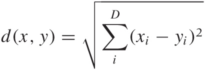
where the sum is running over all dimensions—then it turns out that we can invert this relationship explicitly and find expressions for the coordinates in terms of the distances. (The only additional assumption we need to make is that the center of mass of the entire data set lies at the origin, but this amounts to no more than an arbitrary translation of all points.) This technique is known as classical or metric scaling.
The situation is more complicated if we cannot assume that the distance measure is Euclidean. Now we can no longer invert the relationship exactly and must resort instead to iterative approximation schemes. Because the resulting coordinates may not replicate the original distances exactly, we include an additional constraint: the distance matrix calculated from the new positions must obey the same rank order as the original distance matrix: if the original distances between any three points obeyed the relationship d(x, y) < d(x, z), then the calculated coordinates of the three points must satisfy this also. For this reason, this version of multidimensional scaling is known as ordinal scaling.
The basic algorithm makes an initial guess for the coordinates and calculates a distance matrix based on the guessed coordinates. The coordinates are then changed iteratively to minimize the discrepancy (known as the “stress”) between the new distance matrix and the original one.
Both versions of multidimensional scaling lead to a set of coordinates in the desired number of dimensions (usually two), which we can use to plot the data points in a form of scatter plot. We can then inspect this plot for clusters, outliers, or other features.
Network Graphs
In passing, I’d like to mention force-based algorithms for drawing network graphs because they are similar in spirit to multidimensional scaling.
Imagine we have a network consisting of nodes, some of which are connected by vertices (or edges), and we would like to find a way to plot this network in a way that is “attractive” or “pleasing.” One approach is to treat the edges as springs, in such a way that each spring has a preferred extension and exerts an opposing force—in the direction of the spring—if compressed or extended beyond its preferred length. We can now try to find a configuration (i.e., a set of coordinates for all nodes) that will minimize the overall tension of the springs.
There are basically two ways we can go about this. We can write down the the total energy due to the distorted springs and then minimize it with respect to the node coordinates using a numerical minimization algorithm. Alternatively, we can “simulate” the system by initializing all nodes with random coordinates and then iteratively moving each node in response to the spring forces acting on it. For smaller networks, we can update all nodes at the same time; for very large networks, we may randomly choose a single node at each iteration step for update and continue until the configuration no longer changes. It is easy to see how this basic algorithm can be extended to include richer situations—for instance, edges carrying different weights.
Note that this algorithm makes no guarantees regarding the distances that are maintained between the nodes in the final configuration. It is purely a visualization technique.
Kohonen Maps
Self-organizing maps (SOMs), often called Kohonen maps after their inventor, are different from the techniques discussed so far. In both principal component analysis and multidimensional scaling, we attempted to find a new, more favorable arrangement of points by moving them about in a continuous fashion. When constructing a Kohonen map, however, we map the original data points to cells in a lattice. The presence of a lattice forces a fixed topology on the system; in particular, each point in a lattice has a fixed set of neighbors. (This property is typically and confusingly called “ordering” in most of the literature on Kohonen maps.)
The basic process of constructing a Kohonen map works as follows. We start with a set of k data points in p dimensions, so that each data point consists of a tuple of p numeric values. (I intentionally avoid the word “vector” here because there is no requirement that the data points must satisfy the “mixable” property characteristic of vectors—see Appendix C and Chapter 13.)
Next we prepare a lattice. For simplicity, we consider a two-dimensional square lattice consisting of n × m cells. Each cell contains a p-dimensional tuple, similar to a data point, which is called the reference tuple. We initialize this tuple with random values. In other words, our lattice consists of a collection of random data points, arranged on a regular grid.
Now we perform the following iteration. For each data point, we find that cell in the lattice with the smallest distance between its contained p-tuple and the data point; then we assign the data point to this cell. Note that multiple data points can be assigned to the same cell if necessary.
Once all the data points have been assigned to cells in the lattice, we update the p-tuples of all cells based on the values of the data points assigned to the cell itself and to its neighboring cells. In other words, we use the data points assigned to each cell, as well as those assigned to the cell’s neighbors, to compute a new tuple for the cell.
When all lattice points have been updated, we restart the iteration and begin assigning data points to cells again (after erasing the previous assignments). We stop the iteration if the assignments no longer change or if the differences between the original cell values and their updates are sufficiently small.
This is the basic algorithm for the construction of a Kohonen map. It has certain similarities with the k-means algorithm discussed in Chapter 13. Both are iterative procedures in which data points are assigned to cells or clusters, and the cell or cluster is updated based on the points assigned to it. However, two features are specific to Kohonen maps:
Each data point is mapped to a cell in the lattice, and this implies that each data point is placed in a specific neighborhood of other data points (which have been mapped to neighboring cells).
Because the updating step for each cell relies not only on the current cell but also on neighboring cells, the resulting map will show a “smooth” change of values: changes are averaged or “smeared out” over all cells in the neighborhood. Viewed the other way around, this implies that points that are similar to each other will map to lattice cells that are in close proximity to each other.
Although the basic algorithm seems fairly simple, we still need to decide on a number of technical details if we want to develop a concrete implementation. Most importantly, we still need to give a specific prescription for how the reference tuples will be updated by the data points assigned to the current cell and its neighborhood.
In principle, it would be possible to recalculate the values for the reference tuple from scratch every time by forming a componentwise average of all data points assigned to the cell. In practice, this may lead to instability during iteration, and therefore it is usually recommended to perform an incremental update of the reference value instead, based on the difference between the current value of the reference tuple and the assigned data points. If yi(t) is the value of the reference tuple at position i and at iteration t, then we can write its value at the next iteration step t + 1 as:
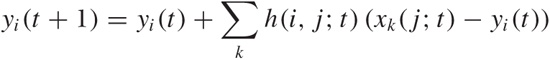
where xk(j; t) is the data point k which has been assigned to lattice point j at iteration step t and where the sum runs over all data points. The weight function h(i, j; t) is now chosen to be a decreasing function of the distance between the lattice cells i and j, and it is also made to shrink in value as the iteration progresses. A typical choice is a Gaussian:
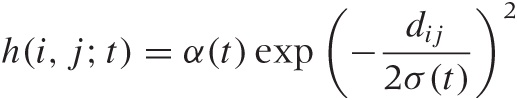
where dij is the Euclidean distance between lattice points i and j and where α(t) and σ(t) are decreasing functions of t. Choices other than the Gaussian are also possible—for instance, we may choose a step function to delimit the effective neighborhood.
Even with these definitions, we still need to decide on further details:
What is the topology of the lattice? Square lattices (like quad-ruled paper) are convenient but strongly single out two specific directions. Hexagonal lattices (like a honeycomb) are more isotropic. We also need to fix the boundary conditions. Do cells at the edge of the lattice have fewer neighbors than cells in the middle of the lattice, or do we wrap the lattice around and connect the opposite edges to form periodic boundary conditions?
What is the size of the lattice? Obviously, the number of cells in the lattice should be smaller than the number of data points (otherwise, we end up with unoccupied cells). But how much smaller? Is there a preferred ratio between data points and lattice cells? Also, should the overall lattice be square (n × n) or rectangular (n × m)? In principle, we can even consider lattices of different shape—triangular, for example, or circular. However, if we choose a lattice of higher symmetry (square or circular), then the orientation of the final result within the lattice is not fixed; for this reason, it has been suggested that the lattice should always be oblongated (e.g., rectangular rather than square).
We need to choose a distance or similarity measure for measuring the distance between data points and reference tuples.
We still need to fix the numerical range of α(t) and σ(t) and define their behavior as functions of t.
In addition, there are many opportunities for low-level tuning, in particular with regard to performance and convergence. For example, we may find it beneficial to initialize the lattice points with values other than random numbers.
Finally, we may ask what we can actually do with the resulting lattice of converged reference tuples. Here are some ideas.
We can use the lattice to form a smooth, “heat map” visualization of the original data set. Because cells in the lattice are closely packed, a Kohonen map interpolates smoothly between different points. This is in contrast to the result from either PCA or MDS, which yield only individual, scattered points.
One problem when plotting a Kohonen map is deciding which feature to show. If the original data set was p-dimensional, you may have to plot p different graphs to see the distribution of all features.
The situation is more favorable if one of the features of interest is categorical and has only a few possible values. In this case, you can plot the labels on the graph and study their relationships (which labels are close to each other, and so on). In this situation, it is also possible to use a “trained” Kohonen map to classify new data points or data points with missing data.
If the number of cells in the lattice was chosen much smaller than the number of original data points, then you can try mapping the reference tuples back into the original data space—for example, to use them as prototypes for clustering purposes.
Kohonen maps are an interesting technique that occupy a space between clustering and dimensionality reduction. Kohonen maps group similar points together like a clustering algorithm, but they also generate a low-dimensional representation of all data points by mapping all points to a low-dimensional lattice. The entire concept is very ad hoc and heuristic; there is little rigorous theory, and thus there is little guidance on the choice of specific details. Nonetheless, the hands-on, intuitive nature of Kohonen maps lends itself to exploration and experimentation in a way that a more rigorous (but also more abstract) technique like PCA does not.
Workshop: PCA with R
Principal component analysis is a complicated technique, so it makes sense to use specialized tools that hide most of the complexity. Here we shall use R, which is the best-known open source package for statistical calculations. (We covered some of the basics of R in the Workshop section of Chapter 10; here I want to demonstrate some of the advanced functionality built into R.)
Let’s consider a nontrivial example. For a collection of nearly 5,000 wines, almost a dozen physico-chemical properties were measured, and the results of a subjective “quality” or taste test were recorded as well.[24] The properties are:
 1 - fixed acidity
 2 - volatile acidity
 3 - citric acid
 4 - residual sugar
 5 - chlorides
 6 - free sulfur dioxide
 7 - total sulfur dioxide
 8 - density
 9 - pH
10 - sulphates
11 - alcohol
12 - quality (score between 0 and 10)
This is a complicated data set, and having to handle 11 input variables is not comfortable. Can we find a way to make sense of them and possibly even find out which are most important in determining the overall quality of the wine?
This is a problem that is perfect for an application of the PCA. And as we will see, R makes this really easy for us.
For this example, I’ll take you on a slightly roundabout route. Be prepared that our initial attempt will lead to an incorrect conclusion! I am including this detour here for a number of reasons. I want to remind you that real data analysis, with real and interesting data sets, usually does not progress linearly. Instead, it is very important that, as we work with a data set, we constantly keep checking and questioning our results as we go along. Do they make sense? Might we be missing something? I also want to demonstrate how R’s interactive programming model facilitates the required exploratory work style: try something and look at the results; if they look wrong, go back and make sure you are on the right track, and so on.
Although it can be scripted for batch operations, R is primarily intended for interactive use, and that is how we will use it here. We first load the data set into a heterogeneous “data frame” and then invoke the desired functions on it. Functions in turn may return data structures themselves that can be used as input to other functions, that can be printed in a human readable format to the screen, or that can be plotted.
R includes many statistical functions as built-in functions. In our specific case, we can perform an entire principal component analysis in a single command:
wine <- read.csv( "winequality-white.csv", sep=';', header=TRUE )
pc <- prcomp( wine )
plot( pc )
This snippet of code reads the data from a file and
assigns the resulting data frame to the variable wine. The prcomp() function performs the actual
principal component analysis and returns a data structure containing
the results, which we assign to the variable pc. We can now examine this returned data
structure in various ways.
R makes heavy use of function overloading—a function such as
plot() will accept different forms
of input and try to find the most useful action to perform, given the
input. For the data structure returned by prcomp(), the plot() function constructs a so-called
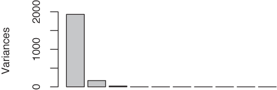
scree plot[25] (see Figure 14-4), showing the
magnitudes of the variances for the various principal components, from
the greatest to the smallest.
We see that the first eigenvalue entirely dominates the
spectrum, suggesting that the corresponding new variable is all that
matters (which of course would be great). To understand in more detail
what is going on, we look at the corresponding eigenvector. The
print() function is another
overloaded function, which for this particular data structure prints
out the eigenvalues and eigenvectors:
print( pc )

(some output omitted...)

                               PC1           PC2           PC3
fixed.acidity        -1.544402e-03 -9.163498e-03 -1.290026e-02
volatile.acidity     -1.690037e-04 -1.545470e-03 -9.288874e-04
citric.acid          -3.386506e-04  1.403069e-04 -1.258444e-03
residual.sugar       -4.732753e-02  1.494318e-02 -9.951917e-01

chlorides            -9.757405e-05 -7.182998e-05 -7.849881e-05
free.sulfur.dioxide  -2.618770e-01  9.646854e-01  2.639318e-02
total.sulfur.dioxide -9.638576e-01 -2.627369e-01  4.278881e-02
density              -3.596983e-05 -1.836319e-05 -4.468979e-04
pH                   -3.384655e-06 -4.169856e-05  7.017342e-03
sulphates            -3.409028e-04 -3.611112e-04  2.142053e-03
alcohol               1.250375e-02  6.455196e-03  8.272268e-02

(some output omitted...)
This is disturbing: if you look closely, you will notice that both the first and the second eigenvector are dominated by the sulfur dioxide concentration—and by a wide margin! That does not seem right. I don’t understand much about wine, but I would not think that the sulfur dioxide content is all that matters in the end.
Perhaps we were moving a little too fast. What do we actually
know about the data in the data set? Right: absolutely nothing! Time
to find out. One quick way to do so is to use the summary() function on the
original data:
summary(wine)
fixed.acidity    volatile.acidity  citric.acid     residual.sugar
Min.   : 3.800   Min.   :0.0800   Min.   :0.0000   Min.   : 0.600
1st Qu.: 6.300   1st Qu.:0.2100   1st Qu.:0.2700   1st Qu.: 1.700
Median : 6.800   Median :0.2600   Median :0.3200   Median : 5.200
Mean   : 6.855   Mean   :0.2782   Mean   :0.3342   Mean   : 6.391
3rd Qu.: 7.300   3rd Qu.:0.3200   3rd Qu.:0.3900   3rd Qu.: 9.900
Max.   :14.200   Max.   :1.1000   Max.   :1.6600   Max.   :65.800
    chlorides     free.sulfur.dioxide total.sulfur.dioxide    density
Min.   :0.00900   Min.   :  2.00       Min.   :  9.0        Min.   :0.9871
1st Qu.:0.03600   1st Qu.: 23.00       1st Qu.:108.0        1st Qu.:0.9917
Median :0.04300   Median : 34.00       Median :134.0        Median :0.9937
Mean   :0.04577   Mean   : 35.31       Mean   :138.4        Mean   :0.9940
3rd Qu.:0.05000   3rd Qu.: 46.00       3rd Qu.:167.0        3rd Qu.:0.9961
Max.   :0.34600   Max.   :289.00       Max.   :440.0        Max.   :1.0390
       pH         sulphates          alcohol           quality
Min.   :2.720   Min.   :0.2200    Min.   : 8.00     Min.   :3.000
1st Qu.:3.090   1st Qu.:0.4100    1st Qu.: 9.50     1st Qu.:5.000
Median :3.180   Median :0.4700    Median :10.40     Median :6.000
Mean   :3.188   Mean   :0.4898    Mean   :10.51     Mean   :5.878
3rd Qu.:3.280   3rd Qu.:0.5500    3rd Qu.:11.40     3rd Qu.:6.000
Max.   :3.820   Max.   :1.0800    Max.   :14.20     Max.   :9.000
I am showing the output in its entire length to give you a sense
of the kind of output generated by R. If you look through this
carefully, you will notice that the two sulfur dioxide columns have
values in the tens to hundreds, whereas all other columns have values
between 0.01 and about 10.0. This explains a lot: the two sulfur
dioxide columns dominate the eigenvalue spectrum simply because they
were measured in units that make the numerical values much larger than
the other quantities. As explained before, if this is the case, then
we need to scale the input variables before
performing the PCA. We can achieve this by passing the scale option to the prcomp() command, like so:
pcx <- prcomp( wine, scale=TRUE )
Before we examine the result of this operation, I’d like to point out something else. If you look really closely, you will notice that the quality column is not what it claims to be. The description of the original data set stated that quality was graded on a scale from 1 to 10. But as we can see from the data summary, only grades between 3 and 9 have actually been assigned. Worse, the first quartile is 5 and the third quartile is 6, which means that at least half of all entries in the data set have a quality ranking of either 5 or 6. In other words, the actual range of qualities is much narrower than we might have expected (given the original description of the data) and is strongly dominated by the center. This makes sense (there are more mediocre wines than outstanding or terrible ones), but it also makes this data set much less interesting because whether a wine will be ranked 5 versus 6 during the sensory testing is likely a toss-up.
We can use the table()
function to see how often each quality ranking occurs in the data set
(remember that the dollar sign is used to select a single column from
the data frame):
table( wine$quality )

 3     4    5    6    7   8     9
20   163 1457 2198  880 175     5
As we suspected, the middling ranks totally dominate the distribution. We might therefore want to change our goal and instead try to predict the outliers, either good or bad, rather than spending too much effort on the undifferentiated middle.
Returning to the results of the scaled PCA, we can look at the
spectrum of eigenvalues for the scaled version by using the summary() function (again, overloaded!) on
the return value of prcomp():
summary( pcx )
Importance of components:
                         PC1   PC2   PC3    PC4    PC5    PC6
Standard deviation     1.829 1.259 1.171 1.0416 0.9876 0.9689
Proportion of Variance 0.279 0.132 0.114 0.0904 0.0813 0.0782
Cumulative Proportion  0.279 0.411 0.525 0.6157 0.6970 0.7752
                         PC7    PC8    PC9    PC10   PC11   PC12
Standard deviation     0.8771 0.8508 0.7460 0.5856 0.5330 0.14307
Proportion of Variance 0.0641 0.0603 0.0464 0.0286 0.0237 0.00171
Cumulative Proportion  0.8393 0.8997 0.9460 0.9746 0.9983 1.00000
No single eigenvalue dominates now, and the first 5 (out of 12) eigenvalues account for only 70 percent of the total variance. That’s not encouraging—it doesn’t seem that we can significantly reduce the number of variables this way.
As a last attempt, we can create a biplot. This, too, is very simple; all we need to do is execute (see Figure 14-5)
biplot( pcx )
This is actually a fascinating graph! We see that three of the original variables—alcohol content, sugar content, and density—are parallel to the first principal component (the horizontal axis). Moreover, alcohol content is aligned in the direction opposite to the other two quantities.
But this makes utmost sense. If you recall from chemistry class, alcohol has a lower density than water, and sugar syrup has a higher density. So the result of the PCA reminds us that density, sugar concentration, and alcohol content are not independent: if you change one, the others will change accordingly. And because these variables are parallel to the first principal component, we can conclude that the overall density of the wine is an important quantity.
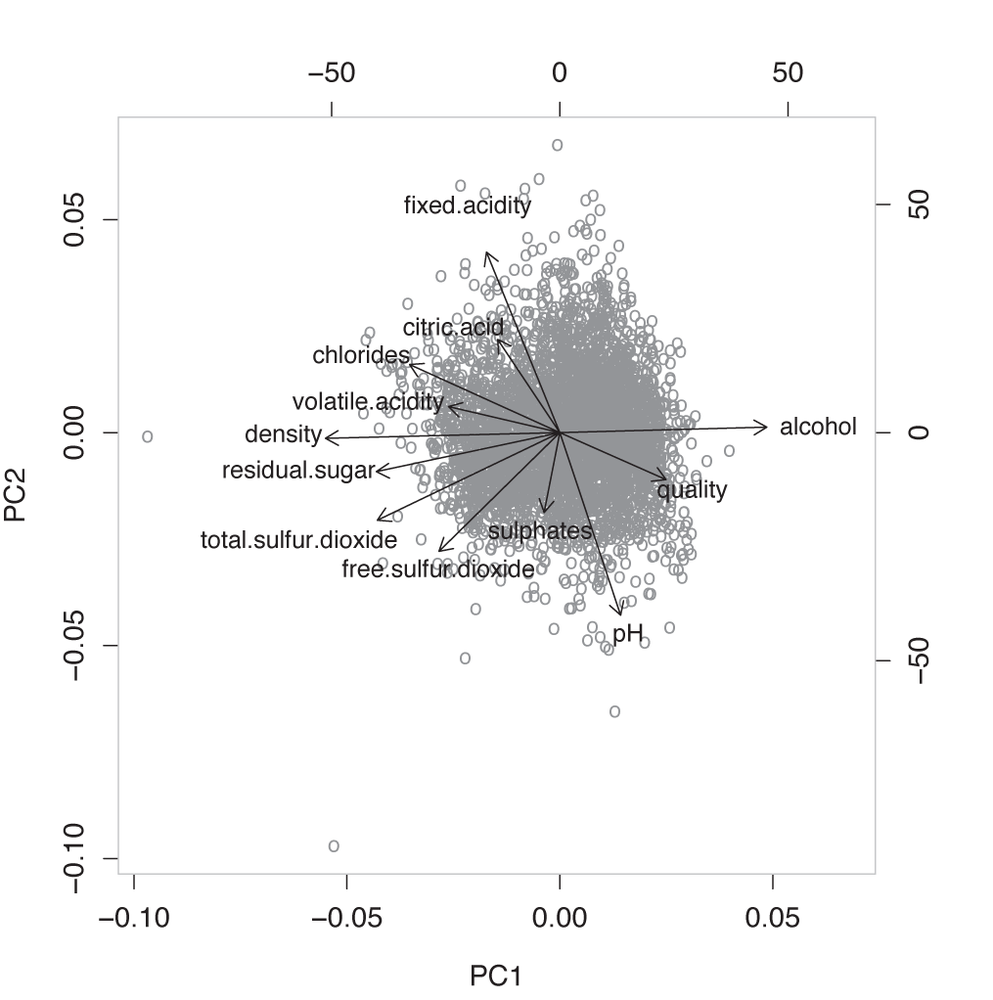
The next set of variables that we can read off are the fixed acidity, the citric acid concentration, and the pH value. Again, this makes sense: the pH is a measure of the acidity of a solution (with higher pH values indicating less acidity). In other words, these three variables are also at least partially redundant.
The odd one out, then, is the overall sulfur content, which is a combination of sulfur dioxide and sulphate concentration.
And finally, it is interesting to see that the quality seems to be determined primarily by the alcohol content and the acidity. This suggests that the more alcoholic and the less sour the wine, the more highly it is ranked—quite a reasonable conclusion!
We could have inferred all of this from the original description of the data set, but I must say that I, for one, failed to see these connections when initially scanning the list of columns. In this sense, the PCA has been a tremendous help in interpreting and understanding the content of the data set.
Finally, I’d like to reflect one more time on our use of R in
this example. This little application demonstrates both the power and
the shortcomings of R. On the one hand, R comes with many high-level,
powerful functions built in, often for quite advanced statistical
techniques (even an unusual and specialized graph like a biplot can be
created with a single command). On the other hand, the heavy reliance
on high-level functions with implicit behavior leads to opaque
programs that make it hard to understand exactly what is going on. For
example, such a critical question as deciding whether or not to
rescale the input data is handled as a rather obscure option to the
prcomp() command. In particular,
the frequent use of overloaded functions—which can exhibit widely
differing functionality depending on their input—makes it hard to
predict the precise outcome of an operation and makes discovering ways
to perform a specific action uncommonly difficult.
Further Reading
Introduction to Multivariate Analysis. Chris Chatfield and Alexander Collins. Chapman & Hall/CRC. 1981.
A bit dated but still one of the most practical, hands-on introductions to the mathematical theory of multivariate analysis. The section on PCA is particularly clear and practical but entirely skips computational issues and makes no mention of the SVD.
Principal Component Analysis. I. T. Jolliffe. 2nd ed., Springer. 2002.
The definitive reference on principal component analysis. Not an easy read.
Multidimensional Scaling. Trevor F. Cox and Michael A. A. Cox. Chapman & Hall/CRC. 2001.
The description of multidimensional scaling given in this chapter is merely a sketch—mostly, because I find it hard to imagine scenarios where this technique is truly useful. However, it has a lot of appeal and is fun to tinker with. Much more information, including some extensions, can be found in this book.
Introduction to Data Mining. Pang-Ning Tan, Michael Steinbach, and Vipin Kumar. Addison-Wesley. 2005.
This is my favorite reference on data mining. The presentation is compact and more technical than in most other books on this topic.
Linear Algebra
Linear algebra is a foundational topic. It is here that one encounters for the first time abstract concepts such as spaces and mappings treated as objects of interest in their own right. It takes time and some real mental effort to get used to these notions, but one gains a whole different perspective on things.
The material is also of immense practical value—particularly its central result, which is the spectral decomposition theorem. The importance of this result cannot be overstated: it is used in every multi-dimensional problem in mathematics, science, and engineering.
However, the material is abstract and unfamiliar, which makes it hard for the beginner. Most introductory books on linear algebra try to make the topic more palatable by emphasizing applications, but that only serves to confuse matters even more, because it never becomes clear why all that abstract machinery is needed when looking at elementary examples. The abstract notions at the heart of linear algebra are best appreciated, and most easily understood, when treated in their own right.
The resources listed here are those I have found most helpful in this regard.
Linear Algebra Done Right. Sheldon Axler. 2nd ed., Springer. 2004. The book lives up to its grandiose title. It treats linear algebra as an abstract theory of mappings but on a very accessible, advanced undergraduate level. Highly recommended but probably not as the first book on the topic.
Matrix Methods in Data Mining and Pattern Recognition. Lars Eldén. SIAM. 2007. This short book is an introduction to linear algebra with a particular eye to applications in data mining. The pace is fast and probably requires at least some previous familiarity with the subject.
Understanding Complex Datasets: Data Mining with Matrix Decompositions. David Skillicorn. Chapman & Hall/CRC. 2007.
An advanced book, concentrating mostly on applications of the SVD and its variants.
“A Singularly Valuable Decomposition: The SVD of a Matrix.” Dan Kalman. The College Mathematics Journal 27 (1996), p. 2. This article, which can be found on the Web, is a nice introduction to the SVD. It’s not for beginners, however.
[24] This example is taken from the “Wine Quality” data set, available at the UCI Machine Learning repository at http://archive.ics.uci.edu/ml/.
[25] Scree is the rubble that collects at the base of mountain cliffs.