Table of Contents for
Data Analysis with Open Source Tools
 Data Analysis with Open Source Tools
Published by
O'Reilly Media, Inc., 2010
Data Analysis with Open Source Tools
Published by
O'Reilly Media, Inc., 2010
- Cover
- Data Analysis with Open Source Tools
- O'Reilly Strata Conference
- Data Analysis with Open Source Tools
- Dedication
- A Note Regarding Supplemental Files
- Preface
- 1. Introduction
- I. Graphics: Looking at Data
- 2. A Single Variable: Shape and Distribution
- 3. Two Variables: Establishing Relationships
- 4. Time As a Variable: Time-Series Analysis
- 5. More Than Two Variables: Graphical Multivariate Analysis
- 6. Intermezzo: A Data Analysis Session
- II. Analytics: Modeling Data
- 7. Guesstimation and the Back of the Envelope
- 8. Models from Scaling Arguments
- 9. Arguments from Probability Models
- 10. What You Really Need to Know About Classical Statistics
- 11. Intermezzo: Mythbusting—Bigfoot, Least Squares, and All That
- III. Computation: Mining Data
- 12. Simulations
- 13. Finding Clusters
- 14. Seeing the Forest for the Trees: Finding Important Attributes
- 15. Intermezzo: When More Is Different
- IV. Applications: Using Data
- 16. Reporting, Business Intelligence, and Dashboards
- 17. Financial Calculations and Modeling
- 18. Predictive Analytics
- 19. Epilogue: Facts Are Not Reality
- A. Programming Environments for Scientific Computation and Data Analysis
- B. Results from Calculus
- C. Working with Data
- D. About the Author
- Index
- About the Author
- Colophon
- Copyright
Chapter 9. Arguments from Probability Models
WHEN MODELING SYSTEMS THAT EXHIBIT SOME FORM OF RANDOMNESS, THE CHALLENGE IN THE MODELING process is to find a way to handle the resulting uncertainty. We don’t know for sure what the system will do—there is a range of outcomes, each of which is more or less likely, according to some probability distribution. Occasionally, it is possible to work out the exact probabilities for all possible events; however, this quickly becomes very difficult, if not impossible, as we go from simple (and possibly idealized systems) to real applications. We need to find ways to simplify life!
In this chapter, I want to take a look at some of the “standard” probability models that occur frequently in practical problems. I shall also describe some of their properties that make it possible to reason about them without having to perform explicit calculations for all possible outcomes. We will see that we can reduce the behavior of many random systems to their “typical” outcome and a narrow range around that.
This is true for many situations but not for all! Systems characterized by power-law distribution functions can not be summarized by a narrow regime around a single value, and you will obtain highly misleading (if not outright wrong) results if you try to handle such scenarios with standard methods. It is therefore important to recognize this kind of behavior and to choose appropriate techniques.
The Binomial Distribution and Bernoulli Trials
Bernoulli trials are random trials that can have only two outcomes, commonly called Success and Failure. Success occurs with probability p, and Failure occurs with probability 1 – p. We further assume that successive trials are independent and that the probability parameter p stays constant throughout.
Although this description may sound unreasonably limiting, in fact many different processes can be expressed in terms of Bernoulli trials. We just have to be sufficiently creative when defining the class of events that we consider “Successes.” A few examples:
Define Heads as Success in n successive tosses of a fair coin. In this case, p = 1/2.
Using fair dice, we can define getting an “ace” as Success and all other outcomes as Failure. In this case, p = 1/6.
We could just as well define not getting an “ace” as Success. In this case, p = 5/6.
Consider an urn that contains b black tokens and r red tokens. If we define drawing a red token as Success, then repeated drawings (with replacement!) from the urn constitute Bernoulli trials with p = r/(r + b).
Toss two identical coins and define obtaining two Heads as Success. Each toss of the two coins together constitutes a Bernoulli trial with p = 1/4.
As you can see, the restriction to a binary outcome is not really limiting: even a process that naturally has more than two possible outcomes (such as throwing dice) can be cast in terms of Bernoulli trials if we restrict the definition of Success appropriately. Furthermore, as the last example shows, even combinations of events (such as tossing two coins or, equivalently, two successive tosses of a single coin) can be expressed in terms of Bernoulli trials.
The restricted nature of Bernoulli trials makes it possible to derive some exact results (we’ll see some in a moment). More importantly, though, the abstraction forced on us by the limitations of Bernoulli trials can help to develop simplified conceptual models of a random process.
Exact Results
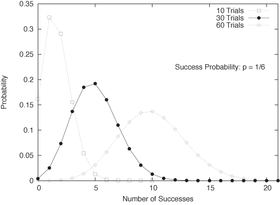
The central formula for Bernoulli trials gives the probability of observing k Successes in N trials with Success probability p, and it is also known as the Binomial distribution (see Figure 9-1):
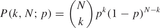
This should make good sense: we need to obtain k Successes, each occurring with probability p, and N – k Failures, each occurring with probability 1 – p. The term:
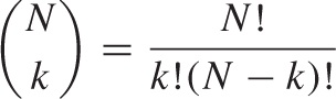
consisting of a binomial coefficient is combinatorial in nature: it gives the number of distinct arrangements for k successes and N – k failures. (This is easy to see. There are N! ways to arrange N distinguishable items: you have N choices for the first item, N – 1 choices for the second, and so on. However, the k Successes are indistinguishable from each other, and the same is true for the N – k Failures. Hence the total number of arrangements is reduced by the number of ways in which the Successes can be rearranged, since all these rearrangements are identical to each other. With k Successes, this means that k! rearrangements are indistinguishable, and similarly for the N – k failures.) Notice that the combinatorial factor does not depend on p.
This formula gives the probability of obtaining a specific number k of Successes. To find the expected number of Successes μ in N Bernoulli trials, we need to average over all possible outcomes:
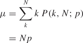
This result should come as no surprise. We use it intuitively whenever we say that we expect “about five Heads in ten tosses of fair coin” (N = 10, p = 1/2) or that we expect to obtain “about ten aces in sixty tosses of a fair die” (N = 60, p = 1/6).
Another result that can be worked out exactly is the standard deviation:
The standard deviation gives us the range over which
we expect the outcomes to vary. (For example, assume that we perform
m experiments, each consisting of
N tosses of a fair coin. The expected number of
Successes in each experiment is Np, but of
course we won’t obtain exactly this number in each experiment.
However, over the course of the m experiments,
we expect to find the number of Successes in the majority of them to
lie between  and
and  .
.
Notice that σ grows more slowly with the number of trials than
does μ (σ ~  versus μ ~ N). The
relative width of the outcome distribution therefore shrinks as we
conduct more trials.
versus μ ~ N). The
relative width of the outcome distribution therefore shrinks as we
conduct more trials.
Using Bernoulli Trials to Develop Mean-Field Models
The primary reason why I place so much emphasis on the concept
of Bernoulli trials is that it lends itself naturally to the
development of mean-field models (see Chapter 8). Suppose we try to
develop a model to predict the staffing level required for a call
center to deal with customer complaints. We know from experience
that about one in every thousand orders will lead to a complaint
(hence p = 1/1000). If we shipped a million
orders a day, we could use the Binomial distribution to work out the
probability to receive 1, 2, 3,..., 999,999, 1,000,000 complaints a
day and then work out the required staffing levels accordingly—a
daunting task! But in the spirit of mean-field theories, we can cut
through the complexity by realizing that we will receive “about
Np = 1,000” complaints a day. So rather than
working with each possible outcome (and its associated probability),
we limit our attention to a single expected
outcome. (And we can now proceed to determine how many calls a
single person can handle per day to find the required number of
customer service people.) We can even go a step further and
incorporate the uncertainty in the number of complaints by
considering the standard deviation, which in this example comes out
to  . (Here I made use of the fact that 1 –
p is very close to 1 for the current value of
p.) The spread is small compared to the
expected number of calls, lending credibility to our initial
approximation of replacing the full distribution with only its
expected outcome. (This is a demonstration for the observation we
made earlier that the width of the resulting distribution grows much
more slowly with N than does the expected value
itself. As N gets larger, this effect becomes
more drastic, which means that mean-field theory gets
better and more reliable the more urgently we
need it! The tough cases can be situations where
N is of moderate size—say, in the range of
10,..., 100. This size is too large to work out all outcomes exactly
but not large enough to be safe working only with the expected
values.)
. (Here I made use of the fact that 1 –
p is very close to 1 for the current value of
p.) The spread is small compared to the
expected number of calls, lending credibility to our initial
approximation of replacing the full distribution with only its
expected outcome. (This is a demonstration for the observation we
made earlier that the width of the resulting distribution grows much
more slowly with N than does the expected value
itself. As N gets larger, this effect becomes
more drastic, which means that mean-field theory gets
better and more reliable the more urgently we
need it! The tough cases can be situations where
N is of moderate size—say, in the range of
10,..., 100. This size is too large to work out all outcomes exactly
but not large enough to be safe working only with the expected
values.)
Having seen this, we can apply similar reasoning to more general situations. For example, notice that the number of orders shipped each day will probably not equal exactly one million—instead, it will be a random quantity itself. So, by using N = 1,000,000 we have employed the mean-field idea already. It should be easy to generalize to other situations from here.
The Gaussian Distribution and the Central Limit Theorem
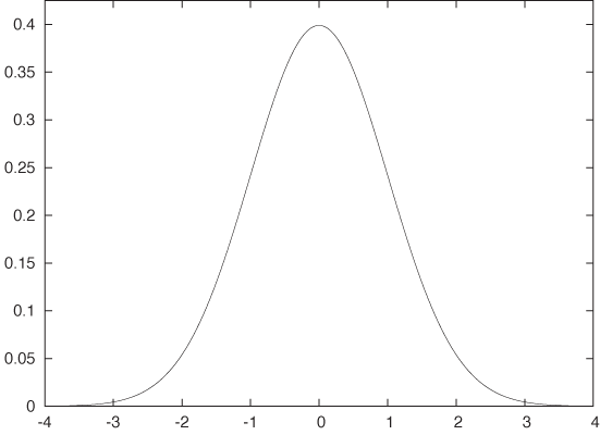
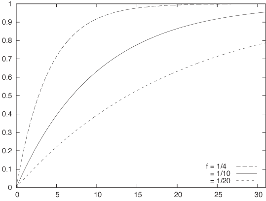
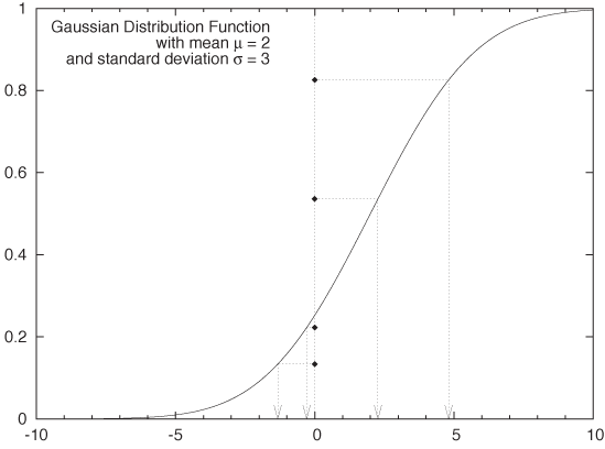
Probably the most ubiquitous formula in all of probability theory and statistics is:
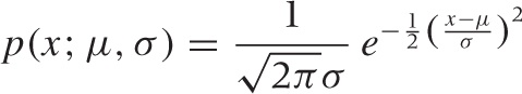
This is the formula for the Gaussian (or Normal) probability density. This is the proverbial “Bell Curve.” (See Figure 9-2 and Appendix B for additional details.)
Two factors contribute to the elevated importance of the Gaussian distribution: on the foundational side, the Central Limit Theorem guarantees that the Gaussian distribution will arise naturally whenever we take averages (of almost anything). On the sheerly practical side, the fact that we can actually explicitly work out most integrals involving the Gaussian means that such expressions make good building blocks for more complicated theories.
The Central Limit Theorem
Imagine you have a source of data points that are distributed according to some common distribution. The data could be numbers drawn from a uniform random-number generator, prices of items in a store, or the body heights of a large group of people.
Now assume that you repeatedly take a sample of n elements from the source (n random numbers, n items from the store, or measurements for n people) and form the total sum of the values. You can also divide by n to get the average. Notice that these sums (or averages) are random quantities themselves: since the points are drawn from a random distribution, their sums will also be random numbers.
Note that we don’t necessarily know the distributions from which the original points come, so it may seem it would be impossible to say anything about the distribution of their sums. Surprisingly, the opposite is true: we can make very precise statements about the form of the distribution according to which the sums are distributed. This is the content of the Central Limit Theorem.
The Central Limit Theorem states that the sums of a bunch of random quantities will be distributed according to a Gaussian distribution. This statement is not strictly true; it is only an approximation, with the quality of the approximation improving as more points are included in each sample (as n gets larger, the approximation gets better). In practice, though, the approximation is excellent even for quite moderate values of n.
This is an amazing statement, given that we made no assumptions whatsoever about the original distributions (I will qualify this in a moment): it seems as if we got something for nothing! After a moment’s thought, however, this result should not be so surprising: if we take a single point from the original distribution, it may be large or it may be small—we don’t know. But if we take many such points, then the highs and the lows will balance each other out “on average.” Hence we should not be too surprised that the distribution of the sums is a smooth distribution with a central peak. It is, however, not obvious that this distribution should turn out to be the Gaussian specifically.
We can now state the Central Limit Theorem formally. Let {xi} be a sample of size n, having the following properties:
All xn are mutually independent.
All xn are drawn from a common distribution.
The mean μ and the standard deviation σ for the distribution of the individual data points xi are finite.
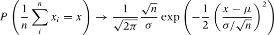
Then the sample average
 is distributed according to a
Gaussian with mean μ and standard deviation
is distributed according to a
Gaussian with mean μ and standard deviation
 . The approximation improves as the sample
size n increases. In other words, the probability of
finding the value x for the sample mean
. The approximation improves as the sample
size n increases. In other words, the probability of
finding the value x for the sample mean
 becomes Gaussian as n
gets large:
becomes Gaussian as n
gets large:
Notice that, as for the binomial distribution, the width of the resulting distribution of the average is smaller than the width of the original distribution of the individual data points. This aspect of the Central Limit Theorem is the formal justification for the common practice to “average out the noise”: no matter how widely the individual data points scatter, their averages will scatter less.
On the other hand, the reduction in width is not as fast as
one might want: it is not reduced linearly with the number
n of points in the sample but only by
. This means that if we take 10 times as many
points, the scatter is reduced to only 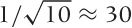 percent of its original value. To reduce it
to 10 percent, we would need to increase the sample size by a factor
of 100. That’s a lot!
percent of its original value. To reduce it
to 10 percent, we would need to increase the sample size by a factor
of 100. That’s a lot!
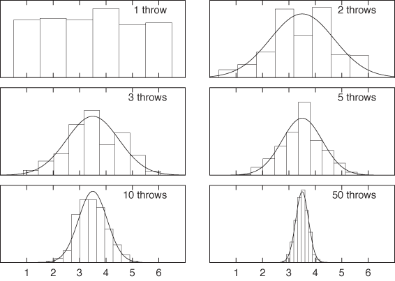
Finally, let’s take a look at the Central Limit Theorem in
action. Suppose we draw samples from a uniform distribution that
takes on the values 1, 2,..., 6 with equal probability—in other
words, throws of a fair die. This distribution has mean μ = 3.5
(that’s pretty obvious) and standard deviation 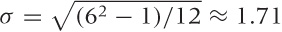 (not as obvious but not terribly hard to work
it out, or you can look it up).
(not as obvious but not terribly hard to work
it out, or you can look it up).
We now throw the die a certain number of times and evaluate the average of the values that we observe. According to the Central Limit Theorem, these averages should be distributed according to a Gaussian distribution that becomes narrower as we increase the number of throws used to obtain an average. To see the distribution of values, we generate a histogram (see Chapter 2). I use 1,000 “repeats” to have enough data for a histogram. (Make sure you understand what is going on here: we throw the die a certain number of times and calculate an average based on those throws; and this entire process is repeated 1,000 times.)
The results are shown in Figure 9-3. In the
upper-left corner we have thrown the die only once and thus form the
“average” over only a single throw. You can see that all of the
possible values are about equally likely: the distribution is
uniform. In the upper-right corner, we throw the dice
twice every time and form the average over both
throws. Already a central tendency in the distribution of the
average of values can be observed! We then
continue to make longer and longer averaging runs. (Also shown is
the Gaussian distribution with the appropriately adjusted width:
 , where n is the number
of throws over which we form the average.)
, where n is the number
of throws over which we form the average.)
I’d like to emphasize two observations in particular. First, note how quickly the central tendency becomes apparent—it only takes averaging over two or three throws for a central peak to becomes established. Second, note how well the properly scaled Gaussian distribution fits the observed histograms. This is the Central Limit Theorem in action.
The Central Term and the Tails
The most predominant feature of the Gaussian density function is the speed with which it falls to zero as |x| (the absolute value of x—see Appendix B) becomes large. It is worth looking at some numbers to understand just how quickly it does decay. For x = 2, the standard Gaussian with zero mean and unit variance is approximately p(2, 0, 1) = 0.05 .... For x = 5, it is already on the order of 10–6; for x = 10 it’s about 10–22; and not much further out, at x = 15, we find p(15, 0, 1) ≈ 10–50. One needs to keep this in perspective: the age of the universe is currently estimated to be about 15 billion years, which is about 4 · 1017 seconds. So, even if we had made a thousand trials per second since the beginning of time, we would still not have found a value as large or larger than x = 10!
Although the Gaussian is defined for all x, its weight is so strongly concentrated within a finite, and actually quite small, interval (about [–5, 5]) that values outside this range will not occur. It is not just that only one in a million events will deviate from the mean by more than 5 standard deviations: the decline continues, so that fewer than one in 1022 events will deviate by more than 10 standard deviations. Large outliers are not just rare—they don’t happen!
This is both the strength and the limitation of the Gaussian model: if the Gaussian model applies, then we know that all variation in the data will be relatively small and therefore “benign.” At the same time, we know that for some systems, large outliers do occur in practice. This means that, for such systems, the Gaussian model and theories based on it will not apply, resulting in bad guidance or outright wrong results. (We will return to this problem shortly.)
Why Is the Gaussian so Useful?
It is the combination of two properties that makes the Gaussian probability distribution so common and useful: because of the Central Limit Theorem, the Gaussian distribution will occur whenever we we dealing with averages; and because so much of the Gaussian’s weight is concentrated in the central region, almost any expression can be approximated by concentrating only on the central region, while largely disregarding the tails.
As we will discuss in Chapter 10 in more detail, the first of these two arguments has been put to good use by the creators of classical statistics: although we may not know anything about the distribution of the actual data points, the Central Limit Theorem enables us to make statements about their averages. Hence, if we concentrate on estimating the sample average of any quantity, then we are on much firmer ground, theoretically. And it is impressive to see how classical statistics is able to make rigorous statements about the extent of confidence intervals for parameter estimates while using almost no information beyond the data points themselves! I’d like to emphasize these two points again: through clever application of the Central Limit Theorem, classical statistics is able to give rigorous (not just intuitive) bounds on estimates—and it can do so without requiring detailed knowledge of (or making additional assumptions about) the system under investigation. This is a remarkable achievement!
The price we pay for this rigor is that we lose much of the richness of the original data set: the distribution of points has been boiled down to a single number—the average.
The second argument is not so relevant from a conceptual point, but it is, of course, of primary practical importance: we can actually do many integrals involving Gaussians, either exactly or in very good approximation. In fact, the Gaussian is so convenient in this regard that it is often the first choice when an integration kernel is needed (we have already seen examples of this in Chapter 2, in the context of kernel density estimates, and in Chapter 4, when we discussed the smoothing of a time series).
Optional: Gaussian Integrals
The basic idea goes like this: we want to evaluate an integral of the form:
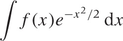
We know that the Gaussian is peaked around x = 0, so that only nearby points will contribute significantly to the value of the integral. We can therefore expand f(x) in a power series for small x. Even if this expansion is no good for large x, the result will not be affected significantly because those points are suppressed by the Gaussian. We end up with a series of integrals of the form
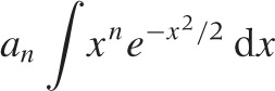
which can be performed exactly. (Here, an is the expansion coefficient from the expansion of f(x).)
We can push this idea even further. Assume that the kernel is not exactly Gaussian but is still strongly peaked:
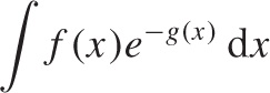
where the function g(x) has a minimum at some location (otherwise, the kernel would not have a peak at all). We can now expand g(x) into a Taylor series around its minimum (let’s assume it is at x = 0), retaining only the first two terms: g(x) ≈ g(0) + g″ (0)x2/2 + ···. The linear term vanishes because the first derivative g′ must be zero at a minimum. Keeping in mind that the first term in this expansion is a constant not depending on x, we have transformed the original integral to one of Gaussian type:
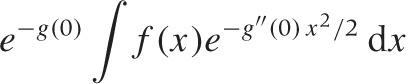
which we already know how to solve.
This technique goes by the name of Laplace’s method (not to be confused with “Gaussian integration,” which is something else entirely).
Beware: The World Is Not Normal!
Given that the Central Limit Theorem is a rigorously proven theorem, what could possibly go wrong? After all, the Gaussian distribution guarantees the absence of outliers, doesn’t it? Yet we all know that unexpected events do occur.
There are two things that can go wrong with the discussion so far:
The Central Limit Theorem only applies to sums or averages of random quantities but not necessarily to the random quantities themselves. The distribution of individual data points may be quite different from a Gaussian, so if we want to reason about individual events (rather than about an aggregate such as their average), then we may need different methods. For example, although the average number of items in a shipment may be Gaussian distributed around a typical value of three items per shipment, there is no guarantee that the actual distribution of items per shipment will follow the same distribution. In fact, the distribution will probably be geometrical, with shipments containing only a single item being much more common than any other shipment size.
More importantly, the Central Limit Theorem may not apply. Remember the three conditions listed as requirements for the Central Limit Theorem to hold? Individual events must be independent, follow the same distribution, and must have a finite mean and standard deviation. As it turns out, the first and second of these conditions can be weakened (meaning that individual events can be somewhat correlated and drawn from slightly different distributions), but the third condition cannot be weakened: individual events must be drawn from a distribution of finite width.
Now this may seem like a minor matter: surely, all distributions occurring in practice are of finite width, aren’t they? As it turns out, the answer is no! Apparently “pathological” distributions of this kind are much more common in real life than one might expect. Such distributions follow power-law behavior, and they are the topic of the next section.
Power-Law Distributions and Non-Normal Statistics
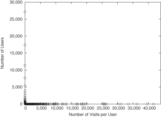
Let’s start with an example. Figure 9-4 shows a histogram for the number of visits per person that a sample of visitors made to a certain website over one month. Two things stand out: the huge number of people who made a handful of visits (fewer than 5 or 6) and, at the other extreme, the huge number of visits that a few people made. (The heaviest user made 41,661 visits: that’s about one per minute over the course of the month—probably a bot or monitor of some sort.)
This distribution looks nothing like the “benign” case in Figure 9-2. The distribution in Figure 9-4 is not merely skewed—it would be no exaggeration to say that it consists entirely of outliers! Ironically, the “average” number of visits per person—calculated naively, by summing the visits and dividing by the number of unique visitors—equals 26 visits per person. This number is clearly not representative of anything: it describes neither the huge majority of light users on the lefthand side of the graph (who made one or two visits), nor the small group of heavy users on the right. (The standard deviation is ±437, which clearly suggests that something is not right, given that the mean is 26 and the number of visits must be positive.)
This kind of behavior is typical for distributions with so-called fat or heavy tails. In contrast to systems ruled by a Gaussian distribution or another distribution with short tails, data values are not effectively limited to a narrow domain. Instead, we can find a nonnegligible fraction of data points that are very far away from the majority of points.
Mathematically speaking, a distribution is heavy-tailed if it falls to zero much slower than an exponential function. Power laws (i.e., functions that behave as ~ 1/xβ for some exponent β > 0) are usually used to describe such behavior.
In Chapter 3, we discussed how to recognize power laws: data points falling onto a straight line on a double logarithmic plot. A double logarithmic plot of the data from Figure 9-4 is shown in Figure 9-5, and we see that eventually (i.e., for more than five visits per person), the data indeed follows a power law (approximately ~ x–1.9). On the lefthand side of Figure 9-5 (i.e., for few visits per person), the behavior is different. (We will come back to this point later.)
Power-law distributions like the one describing the data set in in Figure 9-4 and Figure 9-5 are surprisingly common. They have been observed in a number of different (and often colorful) areas: the frequency with which words are used in texts, the magnitude of earthquakes, the size of files, the copies of books sold, the intensity of wars, the sizes of sand particles and solar flares, the population of cities, and the distribution of wealth. Power-law distributions go by different names in different contexts—you will find them referred to as “Zipf” of “Pareto” distributions, but the mathematical structure is always the same. The term “power-law distribution” is probably the most widely accepted, general term for this kind of heavy-tailed distribution.
Whenever they were found, power-law distributions were met with surprise and (usually) consternation. The reason is that they possess some unexpected and counterintuitive properties:
Observations span a wide range of values, often many orders of magnitude.
There is no typical scale or value that could be used to summarize the distribution of points.
The distribution is extremely skewed, with many data points at the low end and few (but not negligibly few) data points at very high values.
Expectation values often depend on the sample size. Taking the average over a sample of n points may yield a significantly smaller value than taking the average over 2n or 10n data points. (This is in marked contrast to most other distributions, where the quality of the average improves when it is based on more points. Not so for power-law distributions!)
It is the last item that is the most disturbing. After
all, didn’t the Central Limit Theorem tell us that the scatter of the
average was always reduced by a factor of 1/ as the sample size increases? Yes, but remember
the caveat at the end of the last section: the Central Limit Theorem
applies only to those distributions that have a finite mean and
standard deviation. For power-law distributions, this condition is not
necessarily fulfilled, and hence the Central Limit Theorem does
not apply.
The importance of this fact cannot be overstated. Not only does much of our intuition go out the window but most of statistical theory, too! For the most part, distributions without expectations are simply not treated by standard probability theory and statistics.[17]
Working with Power-Law Distributions
So what should you do when you encounter a situation described by a power-law distribution? The most important thing is to stop using classical methods. In particular, the mean-field approach (replacing the distribution by its mean) is no longer applicable and will give misleading or incorrect results.
From a practical point of view, you can try segmenting the data (and, by implication, the system) into different groups: the majority of data points at small values (on the lefthand side in Figure 9-5), the set of data points in the tail of the distribution (for relatively large values), and possibly even a group of data points making up the intermediate regime. Each such group is now more homogeneous, so that standard methods may apply. You will need insight into the business domain of the data, and you should exercise discretion when determining where to make those cuts, because the data itself will not yield a natural “scale” or other quantity that could be used for this purpose.
There is one more practical point that you should be aware of when working with power-law distributions: the form ~ 1/xβ is only valid “asymptotically” for large values of x. For small x, this rule must be supplemented, since it obviously cannot hold for x → 0 (we can’t divide by zero). There are several ways to augment the original form near x = 0. We can either impose a minimum value xmin of x and consider the distribution only for values larger than this. That is often a reasonable approach because such a minimum value may exist naturally. For example there is an obvious “minimum” number of pages (i.e., one page) that a website visitor can view and still be considered a “visitor.” Similar considerations hold for the population of a city and the copies of books sold—all are limited on the left by xmin = 1. Alternatively, the behavior of the observed distribution may be different for small values. Look again at Figure 9-5: for values less than about 5, the curve deviates from the power-law behavior that we find elsewhere.
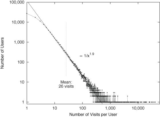
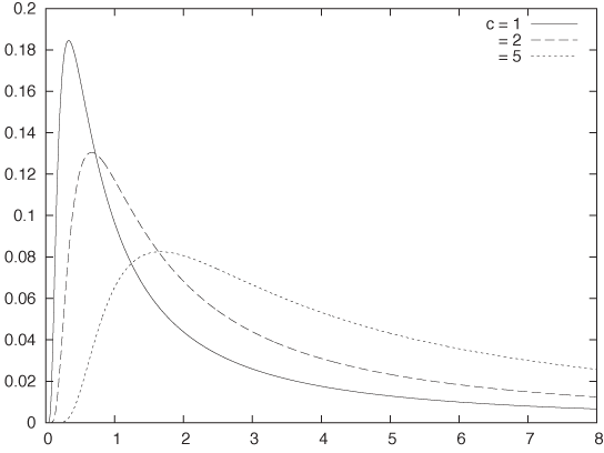
Depending on the shape that we require near zero, we can modify the original rule in different ways. Two examples stand out: if we want a flat peak for x = 0, then we can try a form like ~ 1/(a + xβ) for some a > 0, and if we require a peak at a nonzero location, we can use a distribution like ~ exp(–C/x)/xβ (see Figure 9-6). For specific values of β, two distributions of this kind have special names:
Optional: Distributions with Infinite Expectation Values
The expectation value E(f) of a function f(x), which in turn depends on some random quantity x, is nothing but the weighted average of that function in which we use the probability density p(x) of x as the weight function:
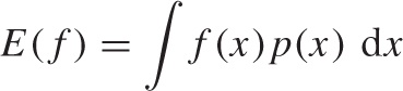
Of particular importance are the expectation values for simple powers of the variable x, the so called moments of the distribution:
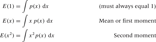
The first expression must always equal 1, because we expect p(x) to be properly normalized. The second is the familiar mean, as the weighted average of x. The last expression is used in the definition of the standard deviation:
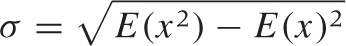
For power-law distributions, which behave as ~ 1/xβ with β > 1 for large x, some of these integrals may not converge—in this case, the corresponding moment “does not exist.” Consider the kth moment (C is the normalization constant C = E(1) = ∫ p(x) dx):
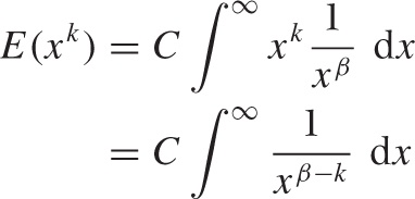
Unless β – k > 1, this integral does not converge at the upper limit of integration. (I assume that the integral is proper at the lower limit of integration, through a lower cutoff xmin or another one of the methods discussed previously.) In particular, if β < 2, then the mean and all higher moments do not exist; if β < 3, then the standard deviation does not exist.
We need to understand that this is an analytical result—it tells us that the distribution is ill behaved and that, for instance, the Central Limit Theorem does not apply in this case. Of course, for any finite sample of n data points drawn from such a distribution, the mean (or other moment) will be perfectly finite. But these analytical results warn us that, if we continue to draw additional data points from the distribution, then their average (or other moment) will not settle down: it will grow as the number of data points in the sample grows. Any summary statistic calculated from a finite sample of points will therefore not be a good estimator for the true (in this case: infinite) value of that statistic. This poses an obvious problem because, of course, all practical samples contain only a finite number of points.
Power-law distributions have no parameters that could (or need) be estimated—except for the exponent, which we know how to obtain from a double logarithmic plot. There is also a maximum likelihood estimator for the exponent:
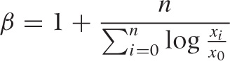
where x0 is the smallest value of x for which the asymptotic power-law behavior holds.
Where to Go from Here
If you want to dig deeper into the theory of heavy-tail phenomena, you will find that it is a mess. There are two reasons for that: on the one hand, the material is technically hard (since one must make do without two standard tools: expectation values and the Central Limit Theorem), so few simple, substantial, powerful results have been obtained—a fact that is often covered up by excessive formalism. On the other hand, the “colorful” and multi disciplinary context in which power-law distributions are found has led to much confusion. Similar results are being discovered and re-discovered in various fields, with each field imposing its own terminology and methodology, thereby obscuring the mathematical commonalities.
The unexpected and often almost paradoxical consequences of power-law behavior also seem to demand an explanation for why such distributions occur in practice and whether they might all be expressions of some common mechanisms. Quite a few theories have been proposed toward this end, but none has found widespread acceptance or proved particularly useful in predicting new phenomena—occasionally grandiose claims to the contrary notwithstanding.
At this point, I think it is fair to say that we don’t understand heavy-tail phenomena: not when and why they occur, nor how to handle them if they do.
Other Distributions
There are some other distributions that describe common scenarios you should be aware of. Some of the most important (or most frequently used) ones are described in this section.
Geometric Distribution
The geometric distribution (see Figure 9-7):
p(k, p) = p(1 – p)k–1 with k = 1, 2, 3,...
is a special case of the binomial distribution. It can be
viewed as the probability of obtaining the first Success at the
kth trial (i.e., after
observing k – 1 failures). Note that there is
only a single arrangement of events for this outcome, hence the
combinatorial factor is equal to one. The geometric distribution has
mean μ = 1/p and standard deviation
 .
.
Poisson Distribution
The binomial distribution gives us the probability of observing exactly k events in n distinct trials. In contrast, the Poisson distribution describes the probability of finding k events during some continuous observation interval of known length. Rather than being characterized by a probability parameter and a number of trials (as for the binomial distribution), the Poisson distribution is characterized by a rate λ and an interval length t.
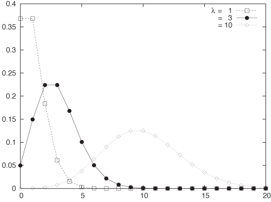
The Poisson distribution p(k, t, λ) gives the probability of observing exactly k events during an interval of length t when the rate at which events occur is λ (see Figure 9-8):
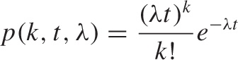
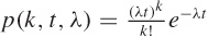
Because t and λ only occur together, this expression is often written in a two-parameter form as p(k, υ) = e–υ υk/k!. Also note that the term e–λt does not depend on k at all—it is merely there as a normalization factor. All the action is in the fractional part of the equation.
Let’s look at an example. Assume that phone calls arrive at a call center at a rate of 15 calls per hour (so that λ = 0.25 calls/minute). Then the Poisson distribution p(k, 1, 0.25) will give us the probability that k = 0, 1, 2,... calls will arrive in any given minute. But we can also use it to calculate the probability that k calls will arrive during any 5-minute time period: p(k, 5, 0.25). Note that in this context, it makes no sense to speak of independent trials: time passes continuously, and the expected number of events depends on the length of the observation interval.
We can collect a few results. Mean μ and standard deviation σ for the Poisson distribution are given by:
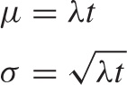
Notice that only a single parameter (λt)
controls both the location and the width of the distribution. For
large λ, the Poisson distribution approaches a Gaussian distribution
with μ = λ and  . Only for small values of λ (say, λ < 20)
are the differences notable. Conversely, to estimate the parameter λ
from observations, we divide the number k of
events observed by the length t of the
observation period: λ =
k/t. Keep in mind that
when evaluating the formula for the Poisson
distribution, the rate λ and the length t of
the interval of interest must be of compatible units. To find the
probability of k calls over 6 minutes in our
call center example above, we can either use t
= 6 minutes and λ = 0.25 calls per minute or t
= 0.1 hours and λ = 15 calls per hour, but we cannot mix them. (Also
note that 6 · 0.25 = 0.1 · 15 = 1.5, as it should.)
. Only for small values of λ (say, λ < 20)
are the differences notable. Conversely, to estimate the parameter λ
from observations, we divide the number k of
events observed by the length t of the
observation period: λ =
k/t. Keep in mind that
when evaluating the formula for the Poisson
distribution, the rate λ and the length t of
the interval of interest must be of compatible units. To find the
probability of k calls over 6 minutes in our
call center example above, we can either use t
= 6 minutes and λ = 0.25 calls per minute or t
= 0.1 hours and λ = 15 calls per hour, but we cannot mix them. (Also
note that 6 · 0.25 = 0.1 · 15 = 1.5, as it should.)
The Poisson distribution is appropriate for processes in which discrete events occur independently and at a constant rate: calls to a call center, misprints in a manuscript, traffic accidents, and so on. However, you have to be careful: it applies only if you can identify a rate at which events occur and if you are interested specifically in the number of events that occur during intervals of varying length. (You cannot expect every histogram to follow a Poisson distribution just because “we are counting events.”)
Log-Normal Distribution
Some quantities are inherently asymmetrical. Consider, for example, the time it takes people to complete a certain task: because everyone is different, we expect a distribution of values. However, all values are necessarily positive (since times cannot be negative). Moreover, we can expect a particular shape of the distribution: there will be some minimum time that nobody can beat, then a small group of very fast champions, a peak at the most typical completion time, and finally a long tail of stragglers. Clearly, such a distribution will not be well described by a Gaussian, which is defined for both positive and negative values of x, is symmetric, and has short tails!
The log-normal distribution is an example of an asymmetric distribution that is suitable for such cases. It is related to the Gaussian: a quantity follows the log-normal distribution if its logarithm is distributed according to a Gaussian.
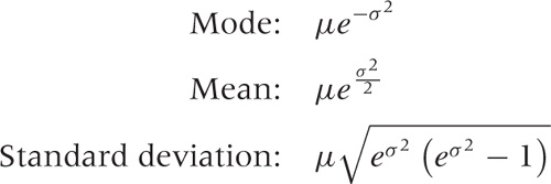
The probability density for the log-normal distribution looks like this:
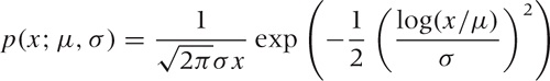
(The additional factor of x in the denominator stems from the Jacobian in the change of variables from x to log x.) You may often find the log-normal distribution written slightly differently:
This is the same once you realize that
log(x/μ) = log(x) – log(μ)
and make the identification 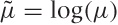 . The first form is much better because it
expresses clearly that μ is the typical scale
of the problem. It also ensures that the argument of the logarithm
is dimensionless (as it must be).
. The first form is much better because it
expresses clearly that μ is the typical scale
of the problem. It also ensures that the argument of the logarithm
is dimensionless (as it must be).
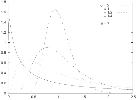
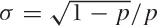
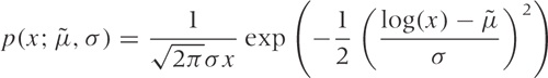
Figure 9-9 shows the log-normal distribution for a few different values of σ. The parameter σ controls the overall “shape” of the curve, whereas the parameter μ controls its “scale.” In general, it can be difficult to predict what the curve will look like for different values of the parameters, but here are some results (the mode is the position of the peak).
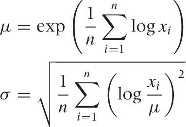
Values for the parameters can be estimated from a data set as follows:
The log-normal distribution is important as an example of a standard statistical distribution that provides an alternative to the Gaussian model for situations that require an asymmetrical distribution. That being said, the log-normal distribution can be fickle to use in practice. Not all asymmetric point distributions are described well by a log-normal distribution, and you may not be able to obtain a good fit for your data using a log-normal distribution. For truly heavy-tail phenomena in particular, you will need a power-law distribution after all. Also keep in mind that the log-normal distribution approaches the Gaussian as σ becomes small compared to μ (i.e., σ/μ ≪ 1), at which point it becomes easier to work with the familiar Gaussian directly.
Special-Purpose Distributions
Many additional distributions have been defined and studied. Some, such as the gamma distribution, are mostly of theoretical importance, whereas others—such as the chi-square, t, and F distributions—are are at the core of classical, frequentist statistics (we will encounter them again in Chapter 10). Still others have been developed to model specific scenarios occurring in practical applications—especially in reliability engineering, where the objective is to make predictions about likely failure rates and survival times.
I just want to mention in passing a few terms that you may encounter. The Weibull distribution is used to express the probability that a device will fail after a certain time. Like the log-normal distribution, it depends on both a shape and a scale parameter. Depending on the value of the shape parameter, the Weibull distribution can be used to model different failure modes. These include “infant mortality” scenarios, where devices are more likely to fail early but the failure rate declines over time as defective items disappear from the population, and “fatigue death” scenarios, where the failure rate rises over time as items age.
Yet another set of distributions goes by the name of extreme-value or Gumbel distributions. They can be used to obtain the probability that the smallest (or largest) value of some random quantity will be of a certain size. In other words, they answer the question: what is the probability that the largest element in a set of random numbers is precisely x?
Quite intentionally, I don’t give formulas for these distributions here. They are rather advanced and specialized tools, and if you want to use them, you will need to consult the appropriate references. However, the important point to take away here is that, for many typical scenarios involving random quantities, people have developed explicit models and studied their properties; hence a little research may well turn up a solution to whatever your current problem is.
Optional: Case Study—Unique Visitors over Time
To put some of the ideas introduced in the last two chapters into practice, let’s look at an example that is a bit more involved. We begin with a probabilistic argument and use it to develop a mean-field model, which in turn will lead to a differential equation that we proceed to solve for our final answer. This example demonstrates how all the different ideas we have been introducing in the last few chapter can fit together to tackle more complicated problems.
Imagine you are running a website. Users visit this website every day of the month at a rate that is roughly constant. We can also assume that we are able to track the identity of these users (through a cookie or something like that). By studying those cookies, we can see that some users visit the site only once in any given month while others visit it several times. We are interested in the number of unique users for the month and, in particular, how this number develops over the course of the month. (The number of unique visitors is a key metric in Internet advertising, for instance.)
The essential difficulty is that some users visit several times during the month, and so the number of unique visitors is smaller than the total number of visitors. Furthermore, we will observe a “saturation effect”: on the first day, almost every user is new; but on the last day of the month, we can expect to have seen many of the visitors earlier in the month already.
We would like to develop some understanding for the number of unique visitors that can be expected for each day of the month (e.g., to monitor whether we are on track to meet some monthly goal for the number of unique visitors). To make progress, we need to develop a model.
To see more clearly, we use the following idealization, which is equivalent to the original problem. Consider an urn that contains N identical tokens (total number of potential visitors). At each turn (every day), we draw k tokens randomly from the urn (average number of visitors per day). We mark all of the drawn tokens to indicate that we have “seen” them and then place them back into the urn. This cycle is repeated for every day of the month.
Because at each turn we mark all unmarked tokens from the random sample drawn at this turn, the number of marked tokens in the urn will increase over time. Because each token is marked at most once, the number of marked tokens in the urn at the end of the month is the number of unique visitors that have visited during that time period.
Phrased this way, the process can be modeled as a sequence of Bernoulli trials. We define drawing an already marked token as Success. Because the number of marked tokens in the urn is increasing, the success probability p will change over time. The relevant variables are:
N | Total number of tokens in urn |
k | Number of tokens drawn at each turn |
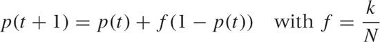
m(t) | Number of already-marked tokens drawn at turn t |
n(t) | Total number of marked tokens in urn at time t |
Probability of drawing an already-marked token at turn t |
Each day consists of a new Bernoulli trial in which k tokens are drawn from the urn. However, because the number of marked tokens in the urn increases every day, the probability p(t) is different every day.
On day t, we have n(t) marked tokens in the urn. We now draw k tokens, of which we expect m(t) = kp(t) to be marked (Successes). This is simply an application of the basic result for the expectation value of Bernoulli trials, using the current value for the probability. (Working with the expectation value in this way constitutes a mean-field approximation.)
The number of unmarked tokens in the current drawing is:
k – m(t) = k – kp(t) = k(1 – p(t))
We now mark these tokens and place them back into the urn, which means that the number of marked tokens in the urn grows by k(1 – p(t)):
n(t + 1) = n(t) + k(1 – p(t))
This equation simply expresses the fact that the new number of marked tokens n(t + 1) consists of the previous number of marked tokens n(t) plus the newly marked tokens k(1 – p(t)).
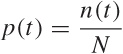
We can now divide both sides by N (the total number of tokens). Recalling that p(t) = n(t)/N, we write:
This is a recurrence relation for p(t), which can be rewritten as:
p(t + 1) – p(t) = f(1 – p(t))
In the continuum limit, we replace the difference between the “new” and the “old” values by the derivative at time t, which turns the recurrence relation into a more convenient differential equation:
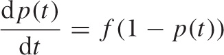
with initial condition p(t = 0) = 0 (because initially there are no marked tokens in the urn). This differential equation has the solution:
p(t) = 1 – e–ft
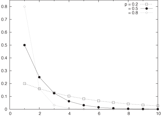
Figure 9-10 shows p(t) for various values of the parameter f. (The parameter f has an obvious interpretation as size of each drawing expressed as a fraction of the total number of tokens in the urn.)
This is the result that we have been looking for. Remember that p(t) = n(t)/N; hence the probability is directly proportional to the number of unique visitors so far. We can rewrite it more explicitly as:
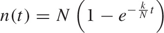
In this form, the equation gives us, for each day of the month, the number of unique visitors for the month up to that date. There is only one unknown parameter: N, the total number of potential visitors. (We know k, the average number of total visitors per day, because this number is immediately available from the web-server logs.) We can now try to fit one or two months’ worth of data to this formula to obtain a value for N. Once we have determined N, the formula predicts the expected number of unique visitors for each day of the month. We can use this information to track whether the actual number of unique visitors for the current month is above or below expectations.
The steps we took in this little example are typical of a lot of modeling. We start with a real problem in a specific situation. To make headway, we recast it in an idealized format that tries to retain only the most relevant information. (In this example: mapping the original problem to an idealized urn model.) Expressing things in terms of an idealized model helps us recognize the problem as one we know how to solve. (Urn models have been studied extensively; in this example, we could identify it with Bernoulli trials, which we know how to handle.) Finding a solution often requires that we make actual approximations in addition to the abstraction from the problem domain to an idealized model. (Working with the expectation value was one such approximation to make the problem tractable; replacing the recurrence relation with a differential equation was another.) Finally, we end up with a “model” that involves some unknown parameters. If we are mostly interested in developing conceptual understanding, then we don’t need to go any further, since we can read off the model’s behavior directly from the formula.
However, if we actually want to make numerical predictions, then we’ll need to find numerical values for those parameters, which is usually done by fitting the model to some already available data. (We should also try to validate the model to see whether it gives a good “fit”; refer to the discussion in Chapter 3 on examining residuals, for instance.)
Finally, I should point out that the model in this example is simplified—as models usually are. The most critical simplification (which would most likely not be correct in a real application) is that every token in the urn has the same probability of being drawn at each turn. In contrast, if look at the behavior of actual visitors, we will find that some are much more likely to visit more frequently while others are less likely to visit. Another simplification is that we assumed the total number of potential visitors to be constant. But if we have a website that sees significant growth from one month to the next, this assumption may not be correct, either. You may want to try and build an improved model that takes these (and perhaps other) considerations into account. (The first one in particular is not easy—in fact, if you succeed, then let me know how you did it!)
Workshop: Power-Law Distributions
The crazy effects of power-law distributions have to be seen to be believed. In this workshop, we shall generate (random) data points distributed according to a power-law distribution and begin to study their properties.
First question: how does one actually generate nonuniformly distributed random numbers on a computer? A random generator that produces uniformly distributed numbers is available in almost all programming environments, but generating random numbers distributed according to some other distribution requires a little bit more work. There are different ways of going about it; some are specific to certain distributions only, whereas others are designed for speed in particular applications. We’ll discuss a simple method that works for distributions that are analytically known.
The starting point is the cumulative distribution function for the distribution in question. By construction, the distribution function is strictly monotonic and takes on values in the interval [0, 1]. If we now generate uniformly distributed numbers between 0 and 1, then we can find the locations at which the cumulative distribution function assumes these values. These points will be distributed according to the desired distribution (see Figure 9-11).
(A good way to think about this is as follows. Imagine you distribute n points uniformly on the interval [0, 1] and find the corresponding locations at which the cumulative distribution function assumes these values. These locations are spaced according to the distribution in question—after all, by construction, the probability grows by the same amount between successive locations. Now use points that are randomly distributed, rather than uniformly, and you end up with random points distributed according to the desired distribution.)
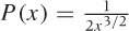
For power-law distributions, we can easily work out the cumulative distribution function and its inverse. Let the probability density p(x) be:
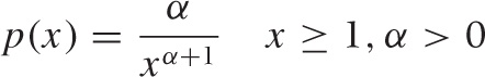
This is known as the the “standard” form of the Pareto distribution. It is valid for values of x greater than 1. (Values of x < 1 have zero probability of occurring.) The parameter α is the “shape parameter” and must be greater than zero, because otherwise the probability is not normalizable. (This is a different convention than the one we used earlier: β = 1 + α.)
We can work out the cumulative distribution function P(x):
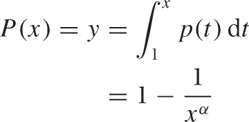
This expression can be inverted to give:
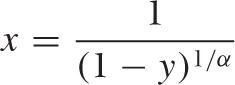
If we now use uniformly distributed random values for y, then the values for x will be distributed according to the Pareto distribution that we started with. (For other distributions, such as the Gaussian, inverting the expression for the cumulative distribution function is often harder, and you may have to find a numerical library that includes the inverse of the distribution function explicitly.)
Now remember what we said earlier. If the exponent in the denominator is less than 2 (i.e., if β ≤ 2 or α ≤ 1), then the “mean does not exist.” In practice, we can evaluate the mean for any sample of points, and for any finite sample the mean will, of course, also be finite. But as we take more and more points, the mean does not settle down—instead it keeps on growing. On the other hand, if the exponent in the denominator is strictly greater than 2 (i.e., if β > 2 or α > 1), then the mean does exist, and its value does not depend on the sample size.
I would like to emphasize again how counterintuitive the behavior for α ≤ 1 is. We usually expect that larger samples will give us better results with less noise. But in this particular scenario, the opposite is true!
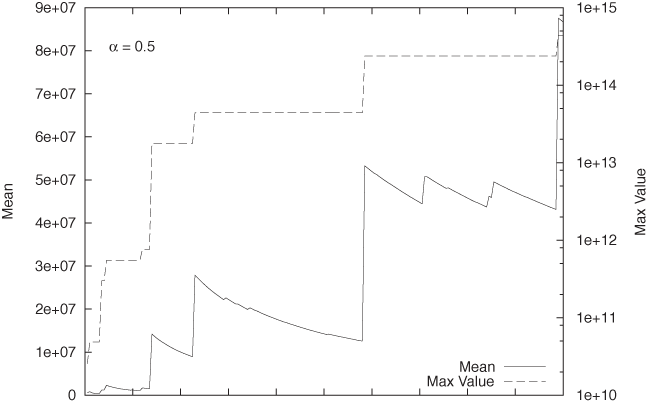
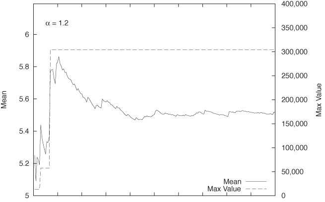
We can explore behavior of this type using the simple program
shown below. All it does is generate 10 million random numbers
distributed according to a Pareto distribution. I generate those
numbers using the method described at the beginning of this section;
alternatively, I could have used the paretovariate() function in the standard
random module. We maintain a
running total of all values (so that we can form the mean) and also
keep track of the largest value seen so far. The results for two runs
with α = 0.5 and α = 1.2 are shown in Figure 9-12 and Figure 9-13,
respectively.
import sys, random

def pareto( alpha ):
    y = random.random()
    return 1.0/pow( 1-y, 1.0/alpha )


alpha = float( sys.argv[1] )

n, ttl, mx = 0, 0, 0

while n<1e7:
    n += 1


    v = pareto( alpha )

    ttl += v
    mx = max( mx, v )

    if( n%50000 == 0 ):
        print n, ttl/n, mx
The typical behavior for situations with α ≤ 1 versus α > 1 is immediately apparent: whereas in Figure 9-13, the mean settles down pretty quickly to a finite value, the mean in Figure 9-12 continues to grow.
We can also recognize clearly what drives this behavior. For α ≤
1, very large values occur relatively frequently. Each such occurrence
leads to an upward jump in the total sum of values seen, which is
reflected in a concomitant jump in the mean. Over time, as more trials
are conducted, the denominator in the mean grows, and hence the value
of the mean begins to fall. However (and this is what is different for
α ≤ 1 versus α > 1), before the mean has fallen back to its
previous value, a further extraordinarily large
value occurs, driving the sum (and hence the mean) up again, with the
consequence that the numerator of the expression ttl/n in the example program grows faster
than the denominator.
You may want to experiment yourself with this kind of system.
The behavior at the borderline value of α = 1 is particularly
interesting. You may also want to investigate how quickly ttl/n grows with different values of α.
Finally, don’t restrict yourself only to the mean. Similar
considerations hold for the standard deviation (see our discussion
regarding this point earlier in the chapter).
Further Reading
An Introduction to Probability Theory and Its Applications, vol. 1. William Feller. 3rd ed., Wiley. 1968.
Every introductory book on probability theory covers most of the material in this chapter. This classic is my personal favorite for its deep, yet accessible treatment and for its large selection of interesting or amusing examples.
An Introduction to Mathematical Statistics and Its Applications. Richard J. Larsen and Morris L. Marx. 4th ed., Prentice Hall. 2005.
This is my favorite book on theoretical statistics. The first third contains a good, practical introduction to many of this chapter’s topics.
NIST/SEMATECH e-Handbook of Statistical Methods. NIST. http://www.itl.nist.gov/div898/handbook/. 2010.
This free ebook is made available by the National Institute for Standards and Technology (NIST). There is a wealth of reliable, high-quality information here.
Statistical Distributions. Merran Evans, Nicholas Hastings, and Brian Peacock. 3rd ed., Wiley. 2000.
This short and accessible reference includes basic information on 40 of the most useful or important probability distributions. If you want to know what distributions exist and what their properties are, this is a good place to start.
“Power Laws, Pareto Distributions and Zipf’s Law.” M. E. J. Newman. Contemporary Physics 46 (2005), p. 323.
This review paper provides a knowledgeable yet very readable introduction to the field of power laws and heavy-tail phenomena. Highly recommended. (Versions of the document can be found on the Web.)
Modeling Complex Systems. Nino Boccara. 2nd ed., Springer. 2010.
Chapter 8 of this book provides a succinct and level-headed overview of the current state of research into power-law phenomena.
[17] The comment on page 48 (out of 440) of Larry Wasserman’s excellent All of Statistics is typical: “From now on, whenever we discuss expectations, we implicitly assume that they exist.”