In the previous section, you learned how to load a raster, perform basic queries, modify it, and save it out as a new file. In this section, you will learn how to create a raster.

A raster is an array of values. So to create one, you start by creating an array, as shown in the following code:

 a_raster=np.array([
 [10,10,1,10,10,10,10],
 [1,1,1,50,10,10,50],
 [10,1,1,51,10,10,50],
 [1,1,1,1,50,10,50]])

The previous code creates a numpy array with four rows of seven columns. Now that you have the array of data, you will need to set some basic properties. The following code will assign the values to variables and then you will pass them to the raster in the following example:

coord=(-106.629773,35.105389)
w=10
h=10
name="BigI.tif"

The following code sets the lower-left corner, width, height, and name for the raster in the variable coord. It then sets the width and height in pixels. Lastly, it names the raster.

The next step is to create the raster by combining the data and properties. The following code will show you how:

d=gdal.GetDriverByName("GTiff")
output=d.Create(name,a_raster.shape[1],a_raster.shape[0],1,gdal.GDT_UInt16)
output.SetGeoTransform((coord[0],w,0,coord[1],0,h))
output.GetRasterBand(1).WriteArray(a_raster)
outsr=osr.SpatialReference()
outsr.ImportFromEPSG(4326)
output.SetProjection(outsr.ExportToWkt())
output.FlushCache()

The previous code assigns the GeoTiff driver to the variable d. Then, it uses the driver to create the raster. The create method takes five parameters—the name, size of x, size of y, the number of bands, and the data type. To get the size of x and y, you can access a_raster.shape, which will return (4,7). Indexing a_raster.shape will give you x and y individually.

Next, the code sets the transformation from map to pixel coordinates using the upper-left corner coordinates and the rotation. The rotation is the width and height, and if it is a north up image, then the other parameters are 0.
To write the data to a band, the code selects the raster band—in this case, you used a single band specified when you called the Create() method, so passing 1 to GetRasterBand() and WriteArray() will take the numpy array.

Now, you will need to assign a spatial reference to the TIF. Create a spatial reference and assign it to outsr. Then, you can import a spatial reference from the EPSG code. Next, set the projection on the TIF by passing the WKT to the SetProjection() method.

The last step is to FlushCache(), which will write the file. If you are done with the TIF, you can set output = None to clear it. However, you will use it again in the following code snippet, so you will skip that step here.

To prove that the code worked, you can check the projection, as shown in the following code:

output.GetProjection()

And the output shows that the TIF is in EPSG:4326:

'GEOGCS["WGS 84",DATUM["WGS_1984",SPHEROID["WGS 84",6378137,298.257223563,AUTHORITY["EPSG","7030"]],AUTHORITY["EPSG","6326"]],PRIMEM["Greenwich",0,AUTHORITY["EPSG","8901"]],UNIT["degree",0.0174532925199433,AUTHORITY["EPSG","9122"]],AUTHORITY["EPSG","4326"]]'

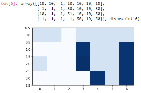
You can display the TIF in Jupyter and see if it looks like you expected. The following code demonstrates how to plot the image and inspect your results:

data=output.ReadAsArray()
w, h =4, 7
image = data.reshape(w,h) #assuming X[0] is of shape (400,) .T
imshow(image, cmap='Blues') #enter bad color to get list
data

The previous code reads the raster as an array and assigns the width and height. It then creates an image variable, reshaping the array to the width and height. Lastly, it passes the image to imshow() and prints the data in the last line. If everything worked, you will see the following image:

The following section will teach you how to use PostgreSQL to work with rasters as an alternative or in conjunction with gdal.