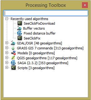
Mastering Geospatial Analysis with Python

QGIS has a processing library. If you go to the Processing menu in QGIS and select Toolbox, you will see a widget displayed with groups of toolboxes. The widget will look as shown:

The processing widget

You have access to the toolboxes in Python by importing processing. You can see the available algorithms by executing the code as follows:

import processing
processing.alglist()

The previous code imports processing and calls the alglist() method. The results are all of the available algorithms from the installed toolboxes. You should see something similar to the following output:

Advanced Python field calculator--------------------->qgis:advancedpythonfieldcalculator
 Bar plot--------------------------------------------->qgis:barplot
 Basic statistics for numeric fields------------------>qgis:basicstatisticsfornumericfields
 Basic statistics for text fields--------------------->qgis:basicstatisticsfortextfields
 Boundary--------------------------------------------->qgis:boundary
 Bounding boxes--------------------------------------->qgis:boundingboxes
 Build virtual vector--------------------------------->qgis:buildvirtualvector
 Check validity--------------------------------------->qgis:checkvalidity
 Clip------------------------------------------------->qgis:clip

To search the algorithms by keyword, you can pass a string to alglist() as in the following code:

Processing.alglist("buffer")

The previous code passes a string to narrow the results. The output will be several algorithms containing the word buffer. See the output as follows:

Fixed distance buffer-------------------------------->qgis:fixeddistancebuffer
 Variable distance buffer----------------------------->saga:shapesbufferattributedistance
 Buffer vectors--------------------------------------->gdalogr:buffervectors
 v.buffer.column - Creates a buffer around features of given type.--->grass:v.buffer.column

In this section, we will use the Buffer vectors algorithm. To see how the algorithm works, you can run the code as follows:

processing.alghelp("gdalogr:buffervectors")

The previous code calls alghelp() and passes the name of the algorithm found in the second column of the alglist(). The result will tell you the parameters and their type required for executing the algorithm. The output is shown as follows:

ALGORITHM: Buffer vectors
 INPUT_LAYER <ParameterVector>
 GEOMETRY <ParameterString>
 DISTANCE <ParameterNumber>
 DISSOLVEALL <ParameterBoolean>
 FIELD <parameters from INPUT_LAYER>
 MULTI <ParameterBoolean>
 OPTIONS <ParameterString>
 OUTPUT_LAYER <OutputVector>

If you run the algorithm from the GUI and then open \.qgis2\processing\processing.log, you will see the parameters used to execute the algorithm. Copy them and use them in your Python code.

The previous output shows the parameters needed to run the algorithm. By using runalg() you can execute the algorithm. The buffer vector is executed in the code as follows:

processing.runalg("gdalogr:buffervectors",r'C:/Users/Paul/Desktop/Projected.shp',"geometry",100,False,None,False,"",r'C:/Users/Paul/Desktop
/ProjectedBuffer.shp') 
layer = iface.addVectorLayer(r'C:\Users\Paul\Desktop\
ProjectedBuffer.shp', "Buffer", "ogr")

The previous code calls runalg() and passes the name of the algorithm we want to run, then the parameters required by the algorithm. In this case:

INPUT_LAYER = Projected.shp
 GEOMETRY = geometry
 DISTANCE = 100
 DISSOLVEALL = False
 FIELD = None
 MULTI = False
 OPTIONS = “”
 OUTPUT_LAYER = ProjectedBuffer.shp

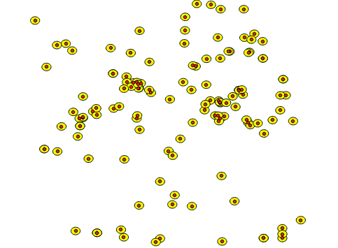
The output layer is then added to the map. The result is shown in the following screenshot:

Results of the buffer algorithm

Now that you know how to use the Python console and call an algorithm let's write our own algorithm. The next section will show you how to make a toolbox that you can call using runalg() or by using the GUI.

Table of Contents for
Mastering Geospatial Analysis with Python

Using toolboxes in Python

Table of Contents for Mastering Geospatial Analysis with Python

Table of Contents for
Mastering Geospatial Analysis with Python