It's time for some hands-on exercises. We'll start with reading and writing some vector data in the form of GeoJSON using the GeoPandas library, which is the application used to demonstrate all examples is Jupyter Notebook, which comes preinstalled with Anaconda3. If you've installed all geospatial Python libraries from Chapter 2, Introduction to Geospatial Code Libraries, you're good to go. If not, do this first. You might decide to create virtual environments for different combinations of Python libraries because of different dependencies and versioning. Open up a new Jupyter Notebook and a browser window and head over to http://www.naturalearthdata.com/downloads/ and download the Natural Earth quick start kit at a convenient location. We'll examine some of that data for the rest of this chapter, along with some other geographical data files.

First, type the following code in a Jupyter Notebook with access to the GeoPandas library and run the following code:

In: import geopandas as gpd
    df = gpd.read_file(r'C:\data\gdal\NE\10m_cultural
    \ne_10m_admin_0_boundary_lines_land.shp')
    df.head()

The output looks as follows:

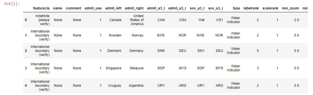
The code does the following—the first line imports the GeoPandas library and shortens its name, saving space whenever we reference it later. The second line reads the data on disk, in this case, a shapefile with land boundary lines. It is assigned to a dataframe variable, which refers to a pandas dataframe, namely a 2D object comparable to an Excel table with rows and columns. The data structures of GeoPandas mimic are subclasses from those of pandas and are named differently—the pandas dataframe in GeoPandas is called a GeoDataFrame. The third line prints the attribute table, which is limited to the first five rows. After running the code, a separate cell's output will list the attribute data from the referenced shapefile. You'll notice that the FID column has no name and that a geometry column has been added as the last column.

This is not the only command to read data, as you can also read data from a PostGIS database, by using the read_postgis() command. Next, we'll plot the data inside our Jupyter Notebook:

In: %matplotlib inline
    df.plot(color='black')

The output of the previous code is as follows:

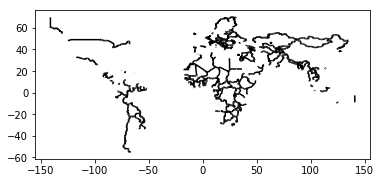
The first line is a so-called magic command, only to be used inside a Jupyter Notebook, and tells it to use the plotting capabilities of the matplotlib library inside a cell of the Jupyter Notebook app. This way, you can plot map data directly as opposed to working with an IDE. The second line states that we want the dataframe plotted, in black (the default color is blue). The output resembles a world map with only land borders, which are visible as black lines.

Next, we'll investigate some of the attributes of GeoPandas data objects:

In: df.geom_type.head()

Out: 0 LineString
     1 LineString
     2 MultiLineString
     3 LineString
     4 LineString
     dtype: object

This tells us that the first five entries in our attribute table are made of line strings and multiline strings. For printing all entries, use the same line of code, without .head():

In: df.crs

Out: {'init': 'epsg:4326'}

The crs attribute refers to the coordinate reference system (CRS) of the dataframe, in this case, epsg:4326, a code defined by the International Association of Oil and Gas Producers (IOGP). Go to www.spatialreference.org for more information on EPSG. The CRS offers essential information about your spatial dataset. EPSG 4326 is also known as WGS 1984, a standard coordinate system for the Earth.

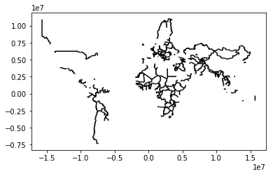
You can change the CRS as follows to a Mercator projection, showing a more vertically stretched image:

In: merc = df.to_crs({'init': 'epsg:3395'})
    merc.plot(color='black')

The output of the previous code is as follows:

Suppose we want to convert the shapefile data of our dataframe into json. GeoPandas does this in one line of code, and the output is listed in a new cell:

In: df.to_json()

This previous command converted the data to a new format but did not write it to a new file. Writing your dataframe to a new geojson file can be done like this:

In: df.to_file(driver='GeoJSON',filename=r'C:\data\world.geojson')

Don't be confused by JSON file extensions—a JSON file with spatial data is a GeoJSON file, even though there's also a separate .geojson file extension.

For file conversion, GeoPandas relies on the Fiona library. To list all available drivers (a software component that lets the operating system and a device communicate with each other), use the following command:

In: import fiona; fiona.supported_drivers