Modern Assembly Language Programming with the ARM Processor

10.9.8 Count Bits

These instructions can be used to count leading sign bits or zeros, or to count the number of bits that are set for each element in a vector:

vcls Count Leading Sign Bits

vclz Count Leading Zero Bits

vcnt Count Set Bits

Syntax

v<op>.<type> Vd, Vm

• <op> is either cls, clz or cnt.

• The valid choices for <type> are given in the following table:

Opcode	Valid Types
vcls	s8, s16, or s32
vclz	u8, u16, or u32
vcnt	i8

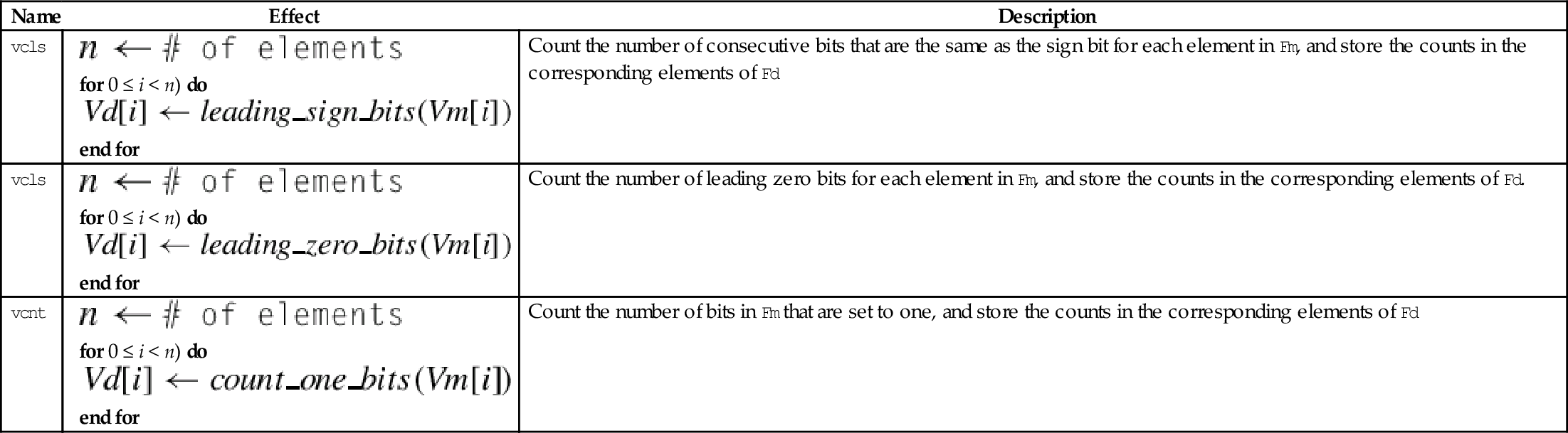
Operations

Name	Effect	Description
vcls	$n \leftarrow # of elements$ for 0 ≤ i < n) do $V d [i] \leftarrow l e a d i n g_s i g n_b i t s (V m [i])$ end for	Count the number of consecutive bits that are the same as the sign bit for each element in Fm, and store the counts in the corresponding elements of Fd
vcls	$n \leftarrow # of elements$ for 0 ≤ i < n) do $V d [i] \leftarrow l e a d i n g_z e r o_b i t s (V m [i])$ end for	Count the number of leading zero bits for each element in Fm, and store the counts in the corresponding elements of Fd.
vcnt	$n \leftarrow # of elements$ for 0 ≤ i < n) do $V d [i] \leftarrow c o u n t_o n e_b i t s (V m [i])$ end for	Count the number of bits in Fm that are set to one, and store the counts in the corresponding elements of Fd

t0260

Examples

10.10 Multiplication and Division

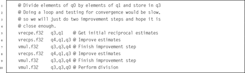
There is no vector divide instruction in NEON. Division is accomplished with multiplication by the reciprocals of the divisors. The reciprocals are found by making an initial estimate, then using the Newton-Raphson method to improve the approximation. This can actually be faster than using a hardware divider. NEON supports single precision floating point and unsigned fixed point reciprocal calculation. Fixed point reciprocals provide higher precision. Division using the NEON reciprocal method may not provide the best precision possible. If the best possible precision is required, then the VFP divide instruction should be used.

10.10.1 Multiply

These instructions are used to multiply the corresponding elements from two vectors:

vmul Multiply

vmla Multiply Accumulate

vmls Multiply Subtract

vmull Multiply Long

vmlal Multiply Accumulate Long

vmlsl Multiply Subtract Long

The long versions can be used to avoid overflow.

Syntax

v<op>.<type> Vd, Vn, Vm

v<op>l.<type> Qd, Dn, Dm

• <op> is either mul, mla. or mls.

• The valid choices for <type> are given in the following table:

Opcode	Valid Types
vmul	p8, i8, i16, or i32
vmla	i8, i16, or i32
vmls	i8, i16, or i32
vmull	p8, s8, s16, s32, u8, u16, or u32
vmlal	s8, s16, s32, u8, u16, or u32
vmlsl	s8, s16, s32, u8, u16, or u32

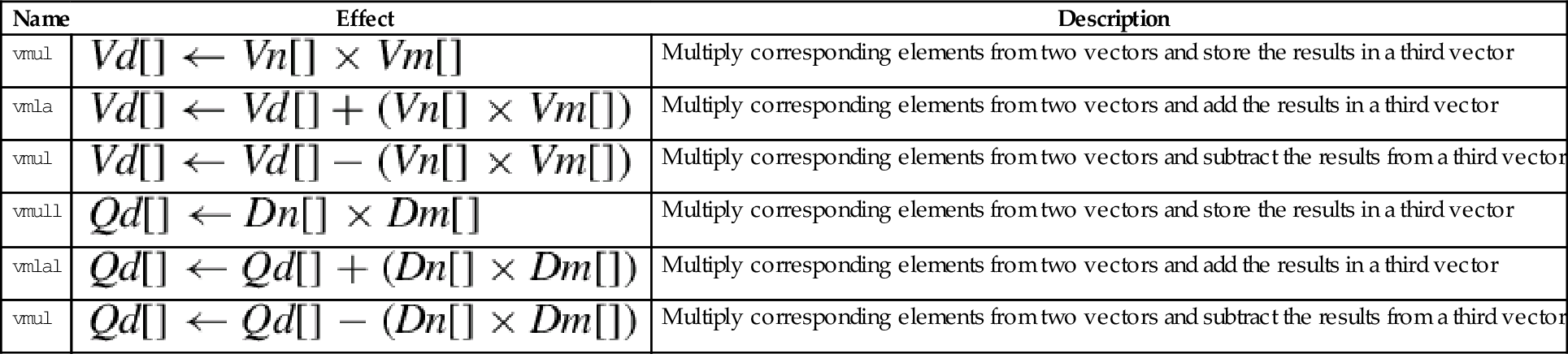
Operations

Name	Effect	Description
vmul	$V d [] \leftarrow V n [] \times V m []$	Multiply corresponding elements from two vectors and store the results in a third vector
vmla	$V d [] \leftarrow V d [] + (V n [] \times V m [])$	Multiply corresponding elements from two vectors and add the results in a third vector
vmul	$V d [] \leftarrow V d [] - (V n [] \times V m [])$	Multiply corresponding elements from two vectors and subtract the results from a third vector
vmull	$Q d [] \leftarrow D n [] \times D m []$	Multiply corresponding elements from two vectors and store the results in a third vector
vmlal	$Q d [] \leftarrow Q d [] + (D n [] \times D m [])$	Multiply corresponding elements from two vectors and add the results in a third vector
vmul	$Q d [] \leftarrow Q d [] - (D n [] \times D m [])$	Multiply corresponding elements from two vectors and subtract the results from a third vector

t0270

Examples

10.10.2 Multiply by Scalar

These instructions are used to multiply each element in a vector by a scalar:

vmul Multiply by Scalar

vmla Multiply Accumulate by Scalar

vmls Multiply Subtract by Scalar

vmull Multiply Long by Scalar

vmlal Multiply Accumulate Long by Scalar

vmlsl Multiply Subtract Long by Scalar

The long versions can be used to avoid overflow.

Syntax

v<op>.<type> Vd, Vn, Dm[x]

v<op>l.<type> Qd, Dn, Dm[x]

• <op> is either mul, mla. or mls.

• The valid choices for <type> are given in the following table:

Opcode	Valid Types
vmul	i16, i32, or f32
vmla	i16, i32, or f32
vmls	i16, i32, or f32
vmull	s16, s32, u16, or u32
vmlal	s16, s32, u16, or u32
vmlsl	s16, s32, u16, or u32

• x must be valid for the chosen <type>.

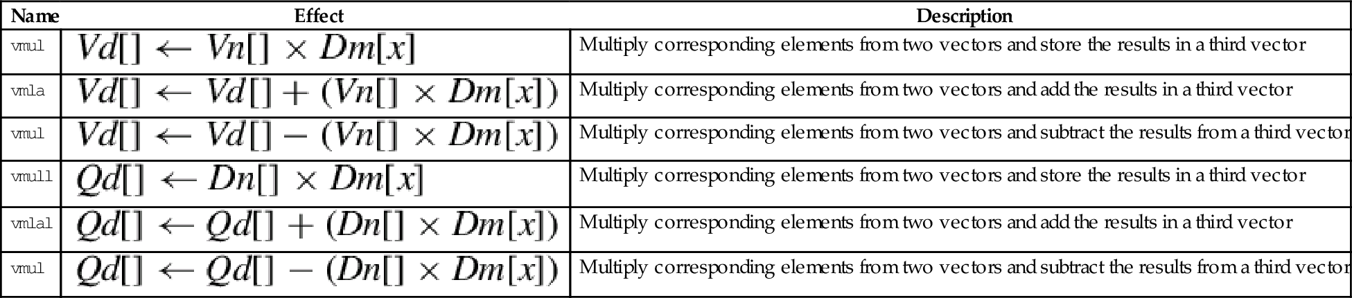
Operations

Name	Effect	Description
vmul	$V d [] \leftarrow V n [] \times D m [x]$	Multiply corresponding elements from two vectors and store the results in a third vector
vmla	$V d [] \leftarrow V d [] + (V n [] \times D m [x])$	Multiply corresponding elements from two vectors and add the results in a third vector
vmul	$V d [] \leftarrow V d [] - (V n [] \times D m [x])$	Multiply corresponding elements from two vectors and subtract the results from a third vector
vmull	$Q d [] \leftarrow D n [] \times D m [x]$	Multiply corresponding elements from two vectors and store the results in a third vector
vmlal	$Q d [] \leftarrow Q d [] + (D n [] \times D m [x])$	Multiply corresponding elements from two vectors and add the results in a third vector
vmul	$Q d [] \leftarrow Q d [] - (D n [] \times D m [x])$	Multiply corresponding elements from two vectors and subtract the results from a third vector

t0280

Examples

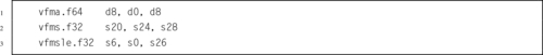
10.10.3 Fused Multiply Accumulate

A fused multiply accumulate operation does not perform rounding between the multiply and add operations. The two operations are fused into one. NEON provides the following fused multiply accumulate instructions:

vfma Fused Multiply Accumulate

vfnma Fused Negate Multiply Accumulate

vfms Fused Multiply Subtract

vfnms Fused Negate Multiply Subtract

Using the fused multiply accumulate can result in improved speed and accuracy for many computations that involve the accumulation of products.

Syntax

<op>{<cond>}.<prec> Fd, Fn, Fm

<op> is one of vfma, vfnma, vfms, or vfnms.

<cond> is an optional condition code.

<prec> may be either f32 or f64.

Operations

Name	Effect	Description
vfma	$F d \leftarrow F d + F n \times F m$	Multiply and accumulate
vnfnma	$F d \leftarrow F d + F n \times - F m$	Negate, multiply, and accumulate
vfms	$F d \leftarrow F d - F n \times F m$	Multiply and subtract
vnfms	$F d \leftarrow F d - F n \times - F m$	Negate multiply, and subtract

Examples

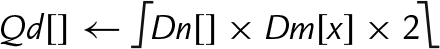
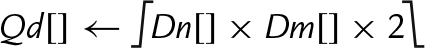
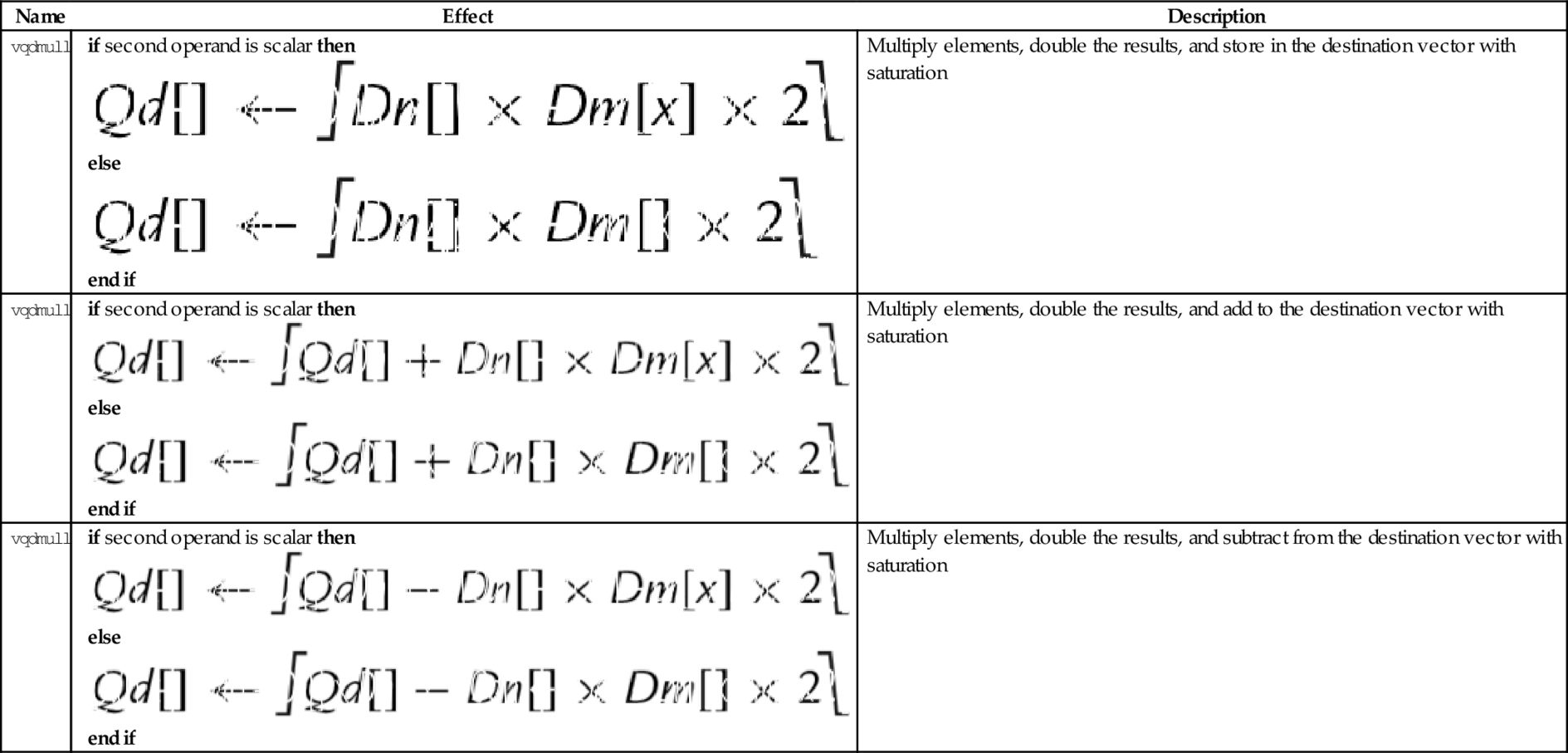
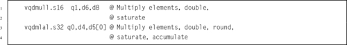
10.10.4 Saturating Multiply and Double (Low)

These instructions perform multiplication, double the results, and perform saturation:

vqdmull Saturating Multiply Double (Low)

vqdmlal Saturating Multiply Double Accumulate (Low)

vqdmlsl Saturating Multiply Double Subtract (Low)

Syntax

vqd<op>l.<type> Qd, Dn, Dm

vqd<op>l.<type> Qd, Dn, Dm[x]

• <op> is either mul, mla. or mls.

• <type> must be either s16 or s32.

Operations

Name	Effect	Description
vqdmull	if second operand is scalar then else end if	Multiply elements, double the results, and store in the destination vector with saturation
vqdmull	if second operand is scalar then else end if	Multiply elements, double the results, and add to the destination vector with saturation
vqdmull	if second operand is scalar then else end if	Multiply elements, double the results, and subtract from the destination vector with saturation

t0290

Examples

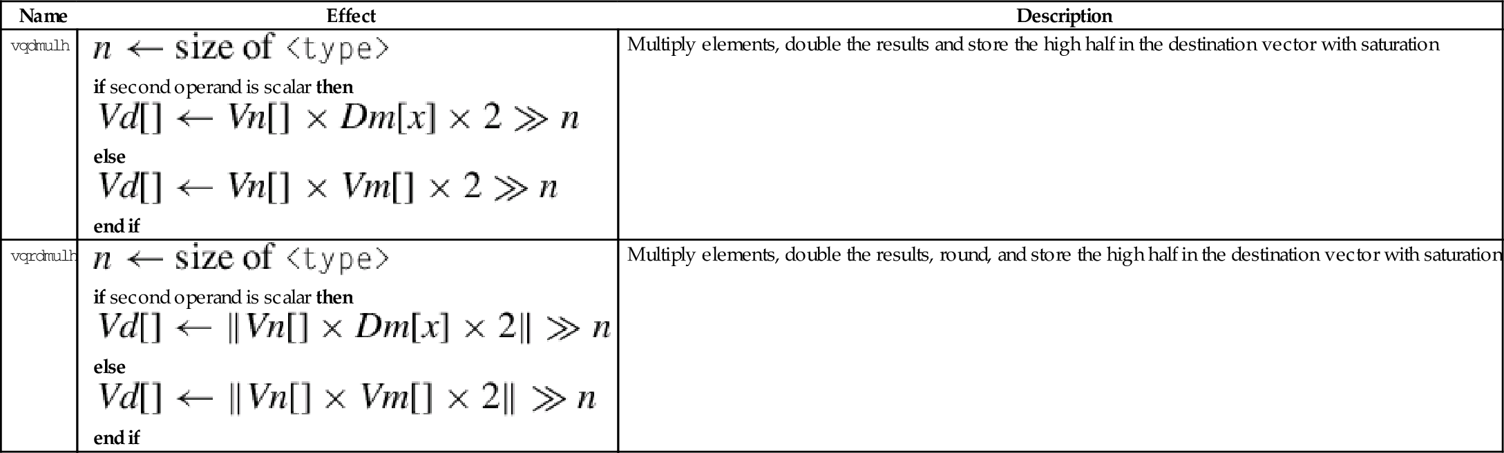
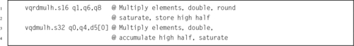
10.10.5 Saturating Multiply and Double (High)

These instructions perform multiplication, double the results, perform saturation, and store the high half of the results:

vqdmulh Saturating Multiply Double (High)

vqrdmulh Saturating Multiply Double (High) and Round

Syntax

vq{r}dmulh.<type> Vd, Vn, Vm

vq{r}dmulh.<type> Vd, Vn, Dm[x]

• <type> must be either s16 or s32.

Operations

Name	Effect	Description
vqdmulh	$n \leftarrow size of <type>$ if second operand is scalar then $V d [] \leftarrow V n [] \times D m [x] \times 2 ≫ n$ else $V d [] \leftarrow V n [] \times V m [] \times 2 ≫ n$ end if	Multiply elements, double the results and store the high half in the destination vector with saturation
vqrdmulh	$n \leftarrow size of <type>$ if second operand is scalar then $V d [] \leftarrow ‖V n [] \times D m [x] \times 2‖ ≫ n$ else $V d [] \leftarrow ‖V n [] \times V m [] \times 2‖ ≫ n$ end if	Multiply elements, double the results, round, and store the high half in the destination vector with saturation

Name

Effect

Description

vqdmulh

$n \leftarrow size of <type>$ si182_e

if second operand is scalar then

$V d [] \leftarrow V n [] \times D m [x] \times 2 ≫ n$ si183_e

else

$V d [] \leftarrow V n [] \times V m [] \times 2 ≫ n$ si184_e

end if

Multiply elements, double the results and store the high half in the destination vector with saturation

vqrdmulh

$n \leftarrow size of <type>$ si182_e

if second operand is scalar then

$V d [] \leftarrow ‖V n [] \times D m [x] \times 2‖ ≫ n$ si186_e

else

$V d [] \leftarrow ‖V n [] \times V m [] \times 2‖ ≫ n$ si187_e

end if

Multiply elements, double the results, round, and store the high half in the destination vector with saturation

t0295

Examples

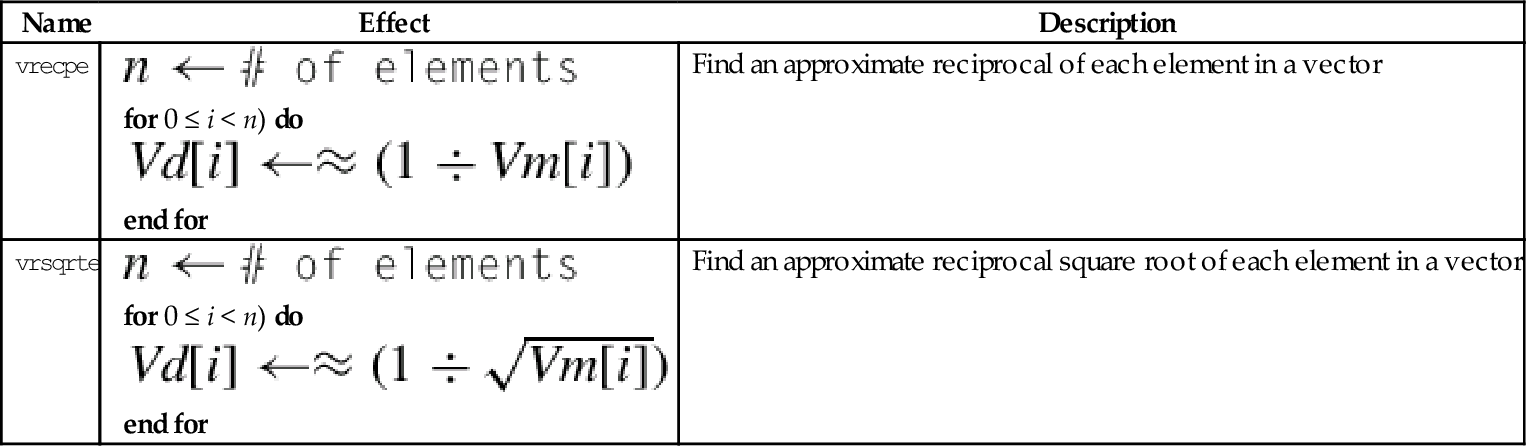
10.10.6 Estimate Reciprocals

These instructions perform the initial estimates of the reciprocal values:

vrecpe Reciprocal Estimate

vrsqrte Reciprocal Square Root Estimate

These work on floating point and unsigned fixed point vectors. The estimates from this instruction are accurate to within about eight bits. If higher accuracy is desired, then the Newton-Raphson method can be used to improve the initial estimates. For more information, see the Reciprocal Step instruction.

Syntax

v<op>.<type> Vd, Vm

• <op> is either recpe or rsqrte.

• <type> must be either u32, or f32.

• If <type> is u32, then the elements are assumed to be U(1,31) fixed point numbers, and the most significant fraction bit (bit 30) must be 1, and the integer part must be zero. The vclz and shift by variable instructions can be used to put the data in the correct format.

• The result elements are always f32.

Operations

Name	Effect	Description
vrecpe	$n \leftarrow # of elements$ for 0 ≤ i < n) do $V d [i] \leftarrow \approx (1 \div V m [i])$ end for	Find an approximate reciprocal of each element in a vector
vrsqrte	$n \leftarrow # of elements$ for 0 ≤ i < n) do $V d [i] \leftarrow \approx (1 \div \sqrt{V m [i]})$ end for	Find an approximate reciprocal square root of each element in a vector

Name

Effect

Description

vrecpe

$n \leftarrow # of elements$ si52_e

for 0 ≤ i < n) do

$V d [i] \leftarrow \approx (1 \div V m [i])$ si189_e

end for

Find an approximate reciprocal of each element in a vector

vrsqrte

$n \leftarrow # of elements$ si52_e

for 0 ≤ i < n) do

$V d [i] \leftarrow \approx (1 \div \sqrt{V m [i]})$ si191_e

end for

Find an approximate reciprocal square root of each element in a vector

t0300

Examples

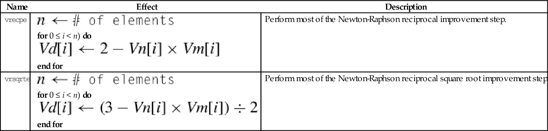
10.10.7 Reciprocal Step

These instructions are used to perform one Newton-Raphson step for improving the reciprocal estimates:

vrecps Reciprocal Step

vrsqrts Reciprocal Square Root Step

For each element in the vector, the following equation can be used to improve the estimates of the reciprocals:

$\begin{array}{l} x_{n + 1} = x_{n} (2 - d x_{n}), \end{array}$

si192_e

where x_n is the estimated reciprocal from the previous step, and d is the number for which the reciprocal is desired. This equation converges to $\frac{1}{d}$ si193_e if x₀ is obtained using vrecpe on d. The vrecps instruction computes

$\begin{array}{l} x_{n + 1}^{'} = 2 - d x_{n}, \end{array}$

si194_e

so one additional multiplication is required to complete the update step. The initial estimate x₀ must be obtained using the vrecpe instruction.

For each element in the vector, the following equation can be used to improve the estimates of the reciprocals of the square roots:

$\begin{array}{l} x_{n + 1} = x_{n} \frac{3 - d x_{n}^{2}}{2}, \end{array}$

si195_e

where x_n is the estimated reciprocal from the previous step, and d is the number for which the reciprocal is desired. This equation converges to $\frac{1}{\sqrt{d}}$ si196_e if x₀ is obtained using vrsqrte on d. The vrsqrts instruction computes

$\begin{array}{l} x_{n + 1}^{'} = \frac{3 - d x_{n}}{2}, \end{array}$

si197_e

so two additional multiplications are required to complete the update step. The initial estimate x₀ must be obtained using the vrsqrte instruction.

Syntax

v<op>.<type> Vd, Vn, Vm

• <op> is either recps or rsqrts.

• <type> must be either u32, or f32.

Operations

Name	Effect	Description
vrecpe	$n \leftarrow # of elements$ for 0 ≤ i < n) do $V d [i] \leftarrow 2 - V n [i] \times V m [i]$ end for	Perform most of the Newton-Raphson reciprocal improvement step.
vrsqrte	$n \leftarrow # of elements$ for 0 ≤ i < n) do $V d [i] \leftarrow (3 - V n [i] \times V m [i]) \div 2$ end for	Perform most of the Newton-Raphson reciprocal square root improvement step

Name

Effect

Description

vrecpe

$n \leftarrow # of elements$ si52_e

for 0 ≤ i < n) do

$V d [i] \leftarrow 2 - V n [i] \times V m [i]$ si199_e

end for

Perform most of the Newton-Raphson reciprocal improvement step.

vrsqrte

$n \leftarrow # of elements$ si52_e

for 0 ≤ i < n) do

$V d [i] \leftarrow (3 - V n [i] \times V m [i]) \div 2$ si201_e

end for

Perform most of the Newton-Raphson reciprocal square root improvement step

t0305

Examples

10.11 Pseudo-Instructions

The GNU assembler supports five pseudo-instructions for NEON. Two of them are vcle and vclt, which were covered in Section 10.6.1. The other three are explained in the following sections.

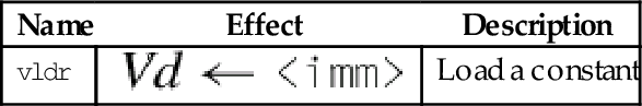
10.11.1 Load Constant

This pseudo-instruction loads a constant value into every element of a NEON vector, or into a VFP single-precision or double-precision register:

vldr Load Constant.

This pseudo-instruction will use vmov if possible. Otherwise, it will create an entry in the literal pool and use vldr.

Syntax

vldr{<cond>}.<type> Vd, =<imm>

• <cond> is an optional condition code.

• <type> must be one of i8, i16, i32, i64, s8, s16, s32, s64, u8, u16, u32, u64, f32, or f64.

• <imm> is a value appropriate for the specified <type>.

Operations

Name	Effect	Description
vldr	$V d \leftarrow <imm>$	Load a constant

t0310

Examples

10.11.2 Bitwise Logical Operations with Immediate Data

It is often useful to clear and/or set specific bits in a register. The following pseudo-instructions can provide bitwise logical operations:

vand Bitwise AND Immediate

vorn Bitwise Complement and OR Immediate

Syntax

v<op>.<type> Vd, #<imm>

• <op> must be either and, or orn.

• V must be either q or d to specify whether the operation involves quadwords or doublewords.

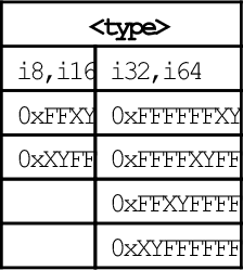
• <type> must be i8, i16, i32, or i64.

• <imm> is a 16-bit or 32-bit immediate value, which is interpreted as a pattern for filling the immediate operand. The following table shows acceptable patterns for <imm>, based on what was chosen for <type>:

<type>
i8,i16	i32,i64
0xFFXY	0xFFFFFFXY
0xXYFF	0xFFFFXYFF
	0xFFXYFFFF
	0xXYFFFFFF

t0315

Operations

Name	Effect	Description
vand	$V d \leftarrow V d \land i m m : i m m \dots$	Logical OR
vorn	$V d \leftarrow \neg (V d \lor i m m : i m m \dots)$	Bit Clear

Examples

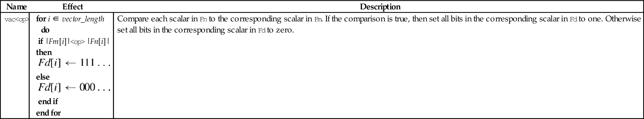
10.11.3 Vector Absolute Compare

The following pseudo-instructions perform comparisons between the absolute values of all of the corresponding elements of two vectors in parallel:

vacle Absolute Compare Less Than or Equal

vaclt Absolute Compare Less Than

The vector absolute compare instruction compares the absolute value of each element of a vector with the absolute value of the corresponding element in a second vector, and sets an element in the destination vector for each comparison. If the comparison is true, then all bits in the result element are set to one. Otherwise, all bits in the result element are set to zero. Note that summing the elements of the result vector (as signed integers) will give the two’s complement of the number of comparisons which were true.

Syntax

vac<op>.f32 Vd, Vn, Vm

• <op> must be either lt or lt.

• V can be d or q.

• The operand element type must be f32.

• The result element type is i32.

Operations

Name	Effect	Description
vac<op>	for i ∈ vector_length do if \|Fm[i]\|<op> \|Fn[i]\| then $F d [i] \leftarrow 111 \dots$ else $F d [i] \leftarrow 000 \dots$ end if end for	Compare each scalar in Fn to the corresponding scalar in Fm. If the comparison is true, then set all bits in the corresponding scalar in Fd to one. Otherwise set all bits in the corresponding scalar in Fd to zero.

Name

Effect

Description

vac<op>

for i ∈ vector_length do

if |Fm[i]|<op> |Fn[i]|

then

$F d [i] \leftarrow 111 \dots$ si89_e

else

$F d [i] \leftarrow 000 \dots$ si90_e

end if

end for

Compare each scalar in Fn to the corresponding scalar in Fm. If the comparison is true, then set all bits in the corresponding scalar in Fd to one. Otherwise set all bits in the corresponding scalar in Fd to zero.

t0325

Examples

10.12 Performance Mathematics: A Final Look at Sine

In Chapter 9, four versions of the sine function were given. Those implementations used scalar and VFP vector modes for single-precision and double-precision. Those previous implementations are already faster than the implementations provided by GCC, However, it may be possible to gain a little more performance by taking advantage of the NEON architecture. All versions of NEON are guaranteed to have a very large register set, and that fact can be used to attain better performance.

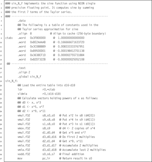
10.12.1 Single Precision

Listing 10.1 shows a single precision floating point implementation of the sine function, using the ARM NEON instruction set. It performs the same operations as the previous implementations of the sine function, but performs many of the calculations in parallel. This implementation is slightly faster than the previous version.

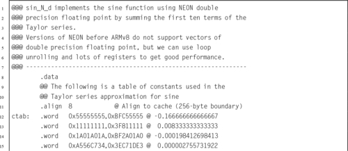
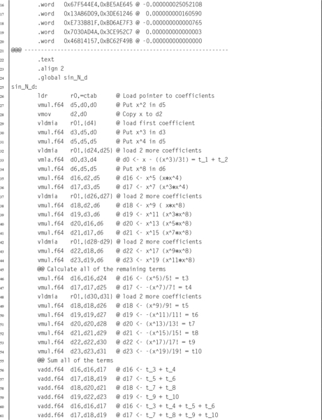
f10-59-9780128036983 — Listing 10.1 NEON implementation of the sin x function using single precision.

10.12.2 Double Precision

Listing 10.2 shows a double precision floating point implementation of the sine function. This code is intended to run on ARMv7 and earlier NEON/VFP systems with the full set of 32 double-precision registers. NEON systems prior to ARMv8 do not have NEON SIMD instructions for double precision operations. This implementation is faster than Listing 9.4 because it uses a large number of registers, does not contain a loop, and is written carefully so that multiple instructions can be at different stages in the pipeline at the same time. This technique of gaining performance is known as loop unrolling.

f10-60a-9780128036983 — Listing 10.2 NEON implementation of the sin x function using double precision.

f10-60b-9780128036983 — Listing 10.2 NEON implementation of the sin x function using double precision.

10.12.3 Performance Comparison

Table 10.4 compares the implementations from Listings 10.1 and 10.2 with the VFP vector implementations from Chapter 9 and the sine function provided by GCC. Notice that in every case, using vector mode VFP instructions is slower than the scalar VFP version. As mentioned previously, vector mode is deprecated on NEON processors. On NEON systems, vector mode is emulated in software. Although vector mode is supported, using it will result in reduced performance, because each vector instruction causes the operating system to take over and substitute a series of scalar floating point operations on-the-fly. A great deal of time was spent by the operating system software in emulating the VFP hardware vector mode.

Table 10.4

Performance of sine function with various implementations

Optimization	Implementation	CPU seconds
None	Single Precision VFP scalar Assembly	1.74
	Single Precision VFP vector Assembly	27.09
	Single Precision NEON Assembly	1.32
	Single Precision C	4.36
	Double Precision VFP scalar Assembly	2.83
	Double Precision VFP vector Assembly	106.46
	Double Precision NEON Assembly	2.24
	Double Precision C	4.59
Full	Single Precision VFP scalar Assembly	1.11
	Single Precision VFP vector Assembly	27.15
	Single Precision NEON Assembly	0.96
	Single Precision C	1.69
	Double Precision VFP scalar Assembly	2.56
	Double Precision VFP vector Assembly	107.5.53
	Double Precision NEON Assembly	2.05
	Double Precision C	4.27

When compiler optimization is not used, the single precision scalar VFP implementation achieves a speedup of about 2.51, and the NEON implementation achieves a speedup of about 3.30 compared to the GCC implementation. The double precision scalar VFP implementation achieves a speedup of about 1.62, and the loop-unrolled NEON implementation achieves a speedup of about 2.05 compared to the GCC implementation.

When the best possible compiler optimization is used (-Ofast), the single precision scalar VFP implementation achieves a speedup of about 1.52, and the NEON implementation achieves a speedup of about 1.76 compared to the GCC implementation. The double precision scalar VFP implementation achieves a speedup of about 1.67, and the loop-unrolled NEON implementation achieves a speedup of about 2.08 compared to the GCC implementation. The single precision NEON version was 1.16 times as fast as the VFP scalar version and the double precision NEON implementation was 1.25 times as fast as the VFP scalar implementation.

Although the VFP versions of the sine function ran without modification on the NEON processor, re-writing them for NEON resulted in significant performance improvement. Performance of the vectorized VFP code running on a NEON processor was abysmal. The take-away lesson is that a programmer can improve performance by writing some functions in assembly that are specifically targeted to run on an specific platform. However, assembly code which improves performance on one platform may actually result in very poor performance on a different platform. To achieve optimal or near-optimal performance, it is important for the programmer to be aware of exactly which hardware platform is being used.

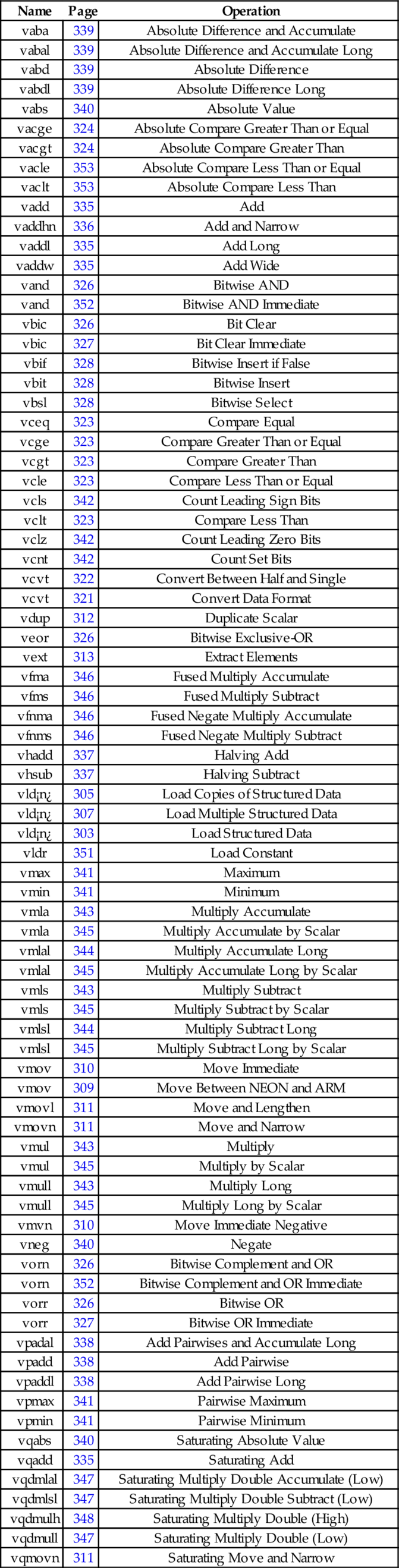
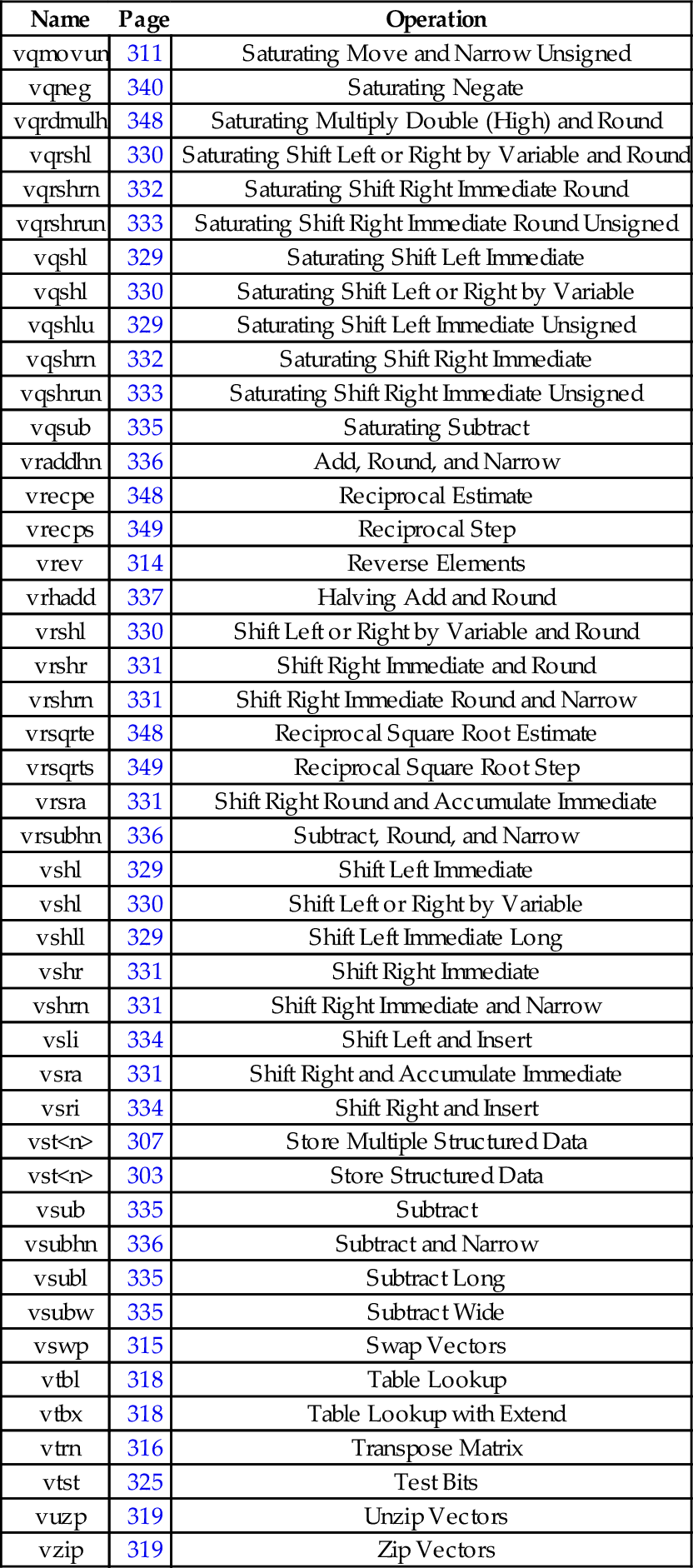
10.13 Alphabetized List of NEON Instructions

Name	Page	Operation
vaba	339	Absolute Difference and Accumulate
vabal	339	Absolute Difference and Accumulate Long
vabd	339	Absolute Difference
vabdl	339	Absolute Difference Long
vabs	340	Absolute Value
vacge	324	Absolute Compare Greater Than or Equal
vacgt	324	Absolute Compare Greater Than
vacle	353	Absolute Compare Less Than or Equal
vaclt	353	Absolute Compare Less Than
vadd	335	Add
vaddhn	336	Add and Narrow
vaddl	335	Add Long
vaddw	335	Add Wide
vand	326	Bitwise AND
vand	352	Bitwise AND Immediate
vbic	326	Bit Clear
vbic	327	Bit Clear Immediate
vbif	328	Bitwise Insert if False
vbit	328	Bitwise Insert
vbsl	328	Bitwise Select
vceq	323	Compare Equal
vcge	323	Compare Greater Than or Equal
vcgt	323	Compare Greater Than
vcle	323	Compare Less Than or Equal
vcls	342	Count Leading Sign Bits
vclt	323	Compare Less Than
vclz	342	Count Leading Zero Bits
vcnt	342	Count Set Bits
vcvt	322	Convert Between Half and Single
vcvt	321	Convert Data Format
vdup	312	Duplicate Scalar
veor	326	Bitwise Exclusive-OR
vext	313	Extract Elements
vfma	346	Fused Multiply Accumulate
vfms	346	Fused Multiply Subtract
vfnma	346	Fused Negate Multiply Accumulate
vfnms	346	Fused Negate Multiply Subtract
vhadd	337	Halving Add
vhsub	337	Halving Subtract
vld¡n¿	305	Load Copies of Structured Data
vld¡n¿	307	Load Multiple Structured Data
vld¡n¿	303	Load Structured Data
vldr	351	Load Constant
vmax	341	Maximum
vmin	341	Minimum
vmla	343	Multiply Accumulate
vmla	345	Multiply Accumulate by Scalar
vmlal	344	Multiply Accumulate Long
vmlal	345	Multiply Accumulate Long by Scalar
vmls	343	Multiply Subtract
vmls	345	Multiply Subtract by Scalar
vmlsl	344	Multiply Subtract Long
vmlsl	345	Multiply Subtract Long by Scalar
vmov	310	Move Immediate
vmov	309	Move Between NEON and ARM
vmovl	311	Move and Lengthen
vmovn	311	Move and Narrow
vmul	343	Multiply
vmul	345	Multiply by Scalar
vmull	343	Multiply Long
vmull	345	Multiply Long by Scalar
vmvn	310	Move Immediate Negative
vneg	340	Negate
vorn	326	Bitwise Complement and OR
vorn	352	Bitwise Complement and OR Immediate
vorr	326	Bitwise OR
vorr	327	Bitwise OR Immediate
vpadal	338	Add Pairwises and Accumulate Long
vpadd	338	Add Pairwise
vpaddl	338	Add Pairwise Long
vpmax	341	Pairwise Maximum
vpmin	341	Pairwise Minimum
vqabs	340	Saturating Absolute Value
vqadd	335	Saturating Add
vqdmlal	347	Saturating Multiply Double Accumulate (Low)
vqdmlsl	347	Saturating Multiply Double Subtract (Low)
vqdmulh	348	Saturating Multiply Double (High)
vqdmull	347	Saturating Multiply Double (Low)
vqmovn	311	Saturating Move and Narrow
vqmovun	311	Saturating Move and Narrow Unsigned
vqneg	340	Saturating Negate
vqrdmulh	348	Saturating Multiply Double (High) and Round
vqrshl	330	Saturating Shift Left or Right by Variable and Round
vqrshrn	332	Saturating Shift Right Immediate Round
vqrshrun	333	Saturating Shift Right Immediate Round Unsigned
vqshl	329	Saturating Shift Left Immediate
vqshl	330	Saturating Shift Left or Right by Variable
vqshlu	329	Saturating Shift Left Immediate Unsigned
vqshrn	332	Saturating Shift Right Immediate
vqshrun	333	Saturating Shift Right Immediate Unsigned
vqsub	335	Saturating Subtract
vraddhn	336	Add, Round, and Narrow
vrecpe	348	Reciprocal Estimate
vrecps	349	Reciprocal Step
vrev	314	Reverse Elements
vrhadd	337	Halving Add and Round
vrshl	330	Shift Left or Right by Variable and Round
vrshr	331	Shift Right Immediate and Round
vrshrn	331	Shift Right Immediate Round and Narrow
vrsqrte	348	Reciprocal Square Root Estimate
vrsqrts	349	Reciprocal Square Root Step
vrsra	331	Shift Right Round and Accumulate Immediate
vrsubhn	336	Subtract, Round, and Narrow
vshl	329	Shift Left Immediate
vshl	330	Shift Left or Right by Variable
vshll	329	Shift Left Immediate Long
vshr	331	Shift Right Immediate
vshrn	331	Shift Right Immediate and Narrow
vsli	334	Shift Left and Insert
vsra	331	Shift Right and Accumulate Immediate
vsri	334	Shift Right and Insert
vst<n>	307	Store Multiple Structured Data
vst<n>	303	Store Structured Data
vsub	335	Subtract
vsubhn	336	Subtract and Narrow
vsubl	335	Subtract Long
vsubw	335	Subtract Wide
vswp	315	Swap Vectors
vtbl	318	Table Lookup
vtbx	318	Table Lookup with Extend
vtrn	316	Transpose Matrix
vtst	325	Test Bits
vuzp	319	Unzip Vectors
vzip	319	Zip Vectors

t0330_a t0330_b

10.14 Chapter Summary

NEON can dramatically improve performance of algorithms that can take advantage of data parallelism. However, compiler support for automatically vectorizing and using NEON instructions is still immature. NEON intrinsics allow C and C++ programmers to access NEON instructions, by making them look like C functions. It is usually just as easy and more concise to write NEON assembly code as it is to use the intrinsics functions. A careful assembly language programmer can usually beat the compiler, sometimes by a wide margin. The greatest gains usually come from converting an algorithm to avoid floating point, and taking advantage of data parallelism.

Exercises

10.1 What is the advantage of using IEEE half-precision? What is the disadvantage?

10.2 NEON achieved relatively modest performance gains on the sine function, when compared to VFP.

(a) Why?

(b) List some tasks for which NEON could significantly outperform VFP.

10.3 There are some limitations on the size of the structure that can be loaded or stored using the vld<n> and vst<n> instructions. What are the limitations?

10.4 The sine function in Listing 10.2 uses a technique known as “loop unrolling” to achieve higher performance. Name at least three reasons why this code is more efficient than using a loop?

10.5 Reimplement the fixed-point sine function from Listing 8.7 using NEON instructions. Hint: you should not need to use a loop. Compare the performance of your NEON implementation with the performance of the original implementation.

10.6 Reimplement Exercise 9.10 using NEON instructions.

10.7 Fixed point operations may be faster than floating point operations. Modify your code from the previous example so that it uses the following definitions for points and transformation matrices:

Use saturating instructions and/or any other techniques necessary to prevent overflow. Compare the performance of the two implementations.

Previous Chapter

Chapter 10: The ARM NEON Extensions

Next Chapter

Part III: Accessing Devices

Table of Contents for Modern Assembly Language Programming with the ARM Processor

10.9.8 Count Bits

Syntax

Operations

Examples

10.10 Multiplication and Division

10.10.1 Multiply

Syntax

Operations

Examples

10.10.2 Multiply by Scalar

Syntax

Operations

Examples

10.10.3 Fused Multiply Accumulate

Syntax

Operations

Examples

10.10.4 Saturating Multiply and Double (Low)

Syntax

Operations

Examples

10.10.5 Saturating Multiply and Double (High)

Syntax

Operations

Examples

10.10.6 Estimate Reciprocals

Syntax

Operations

Examples

10.10.7 Reciprocal Step

Syntax

Operations

Examples

10.11 Pseudo-Instructions

10.11.1 Load Constant

Syntax

Operations

Examples

10.11.2 Bitwise Logical Operations with Immediate Data

Syntax

Operations

Examples

10.11.3 Vector Absolute Compare

Syntax

Operations

Examples

10.12 Performance Mathematics: A Final Look at Sine

10.12.1 Single Precision

10.12.2 Double Precision

10.12.3 Performance Comparison

10.13 Alphabetized List of NEON Instructions

10.14 Chapter Summary

Exercises

Table of Contents for
Modern Assembly Language Programming with the ARM Processor