Table of Contents for
Cryptography and Network Security
 Cryptography and Network Security
Published by
Pearson Education India, 2016
Cryptography and Network Security
Published by
Pearson Education India, 2016
- Cover
- Title Page
- Engineering Chemistry
- Contents
- Foreword - 1
- Foreword - 2
- Preface
- Acknowledgements
- CHAPTER 1 Cryptography
- CHAPTER 2 Mathematics of Modern Cryptography
- CHAPTER 3 Classical Encryption Techniques
- CHAPTER 4 Data Encryption Standard
- Chapter 5 Secure Block Cipher and Stream Cipher Technique
- Chapter 6 Advanced Encryption Standard (AES)187
- Chapter 7 Public Key Cryptosystem
- Chapter 8 Key Management and Key Distribution
- Chapter 9 Elliptic Curve Cryptography
- Chapter 10 Authentication Techniques
- Chapter 11 Digital Signature
- Chapter 12 Authentication Applications
- Chapter 13 Application Layer Security
- Chapter 14 Transport Layer Security
- Chapter 15 IP Security
- Chapter 16 System Security
- Appendix: Frequently Asked University Questions with Solutions
- Basic Mechanical Engineering
Chapter 2
Mathematics of Modern Cryptography
2.1 Basic Number Theory
Number theory is the process of learning the integers and the properties of objects made out of integers (for example, rational numbers) or generalizations of the integers. Number theory plays a vital role in the field of security, memory management, authentication and coding theory. Because, in many cryptographic algorithms used in the field of security, authentication and coding theory, the messages are represented as integer numbers. These integer numbers are converted into some other format before sending it to receiver side. Fermat’s theorem provides a good example of the importance of the number theory. Fermat asked a question that, can prime p be written as the sum of two distinct squares? Yes and the answer is 13. Because, 13 can be written as (13 = 4 + 9, with 4 = 22 and 9 = 32) the sum of two distinct squares. However, the numbers 2 and 11 cannot be written as the sum of two distinct squares.
A prime p = 31415926535897932384626433832795028841 is also the sum of two distinct squares. Because, p = 36847587138599206042 + 42235624485179944052. How do we know that p is prime? To check this, we need to use the computer for the primality test and the two-square decomposition because computers can perform millions of operations per second. Even though we use computers, the computing load to perform this task is extremely high and hence it would take a long period to find such a large prime number. However, the process of finding primality test can be performed in a few seconds by using various algorithms available in number theory. Among the various algorithms, Fermat’s primality test is also one of the efficient method. All these algorithms are included in this chapter under the topic ‘Primality Testing Methods’. This chapter discusses about the overall view of the number theory.
2.1.1 Basic Notations
Given any two integers a and b, the quotient b/a may or may not be an integer. For example,  and
and  . Number theory deals with the first approach, and determines the condition in which one can decide about divisibility of two integers. For example, when a ≠ 0 we say that a divides b if there is another integer k such that b = ka, where k is the quotient. Therefore, a divides b which is denoted as a|b if and only if b = ka.
Lemma: If a|b and a|c, then a|(b + c).
Proof: In order to prove the above lemma, we use a direct proof method. Consider the two integers p and q such that b = pa and c = qa.
Hence, 
Since p + q is an integer, we prove that  .
.
Example 2.1:
Consider the values  . If a divides b and a divides c, prove that a also dives
  for the given three values.
Solution


2.1.2 Congruence
One of the important concepts in number theory is congruences. So, this subsection gives an overview about congruence. Before discussing about congruence, let us know the meaning of equality principle. Two numbers are equal when neither is greater. For example, if x = 8 and y = 8, then we would say that x and y are equal. Similarly, x is congruent (≡) to y(mod n) if and only if (x – y) is a multiple of n. Therefore, two unequal numbers let us say x and y may be congruentially equal under the modulo divison operation. Let x, y and n be integers with n not equal to zero. We say that x ≡ y(mod n) if (x – y) is a multiple of n or n | (x – y).
Examples 2.2:
2.2.1  Because
2.2.2  Because
2.2.3  , Because
2.2.4  Because
Theorem 2.1
If x is congruent to  then
then 
Example 2.3:

Solution
Substitute x, y, n in the congruential equation, 
 , 2 = 2. Since LHS = RHS, 10 is congruent to 2 (mod 4).
Theorem 2.2n
Let n be a positive integer, if  and
and  , then
  and
and  .
.
Example 2.4:
 and
and  then,
then,

Therefore,  because
Similarly,  will also be true.

 because
Theorem 2.3
Let x, y and n be integers with n not equal to zero. We say that [(x mod n) + (y mod n)] mod n = (x + y) mod n.
Theorem 2.4
Let x, y and n be integers with n not equal to zero. We say that [(x mod n) – (y mod n)] mod n = (x – y) mod n.
Theorem 2.5
Let x, y and n be integers with n not equal to zero. We say that [(x mod n) × (y mod n)] mod n = (x × y) mod n.
Example 2.5:
Find the results for Theorems 2.3, 2.4 and 2.5 using the values x = 11, y = 15 and n = 8.
Solution
2.5.1 [(11 mod 8) + (15 mod 8)] mod 8 = 10 mod 8 = 2
Similarly, (11 + 15) mod 8 = 26 mod 8 = 2
2.5.2 [(11 mod 8) – (15 mod 8)] mod 8 = –4 mod 8 = 4
Similarly, (11 – 15) mod 8 = –4 mod 8 = 4
2.5.3 [(11 mod 8) 1 (15 mod 8)] mod 8 = 21 mod 8 = 5
Similarly, (11 1 15) mod 8 = 165 mod 8 = 5
2.1.3 Modular Exponentiation
Exponentiation is a type of operation where two elements are used in which one element is considered as a base element and another element is considered as an exponential element. For example, (xy) is an example of exponential operation where x is a base element and y is an exponential element. When y is a positive integer, exponentiation is performed in a similar way to repeated multiplication is performed. Modular exponentiation is a type of exponentiation in which a modulo division operation is performed after performing an exponentiation operation. For example, (xy mod n), where n is an integer number. The exponentiation is an important concept discussed in many cryptographic algorithms such as RSA, Diffie–Hellman, Elgamal, etc.
Example 2.6:
Find the result of 290 mod 13.
Solution
Step 1: Split x and y into smaller parts using exponent rules as shown below:
 =
=
Step 2: Calculate mod n for each part


Step 3: Use modular multiplication properties to combine these two parts, we have
 =
= 
= 
= 
Memory Efficient Method
In order to reduce the computation complexity of modular exponentiation operation, a memory-efficient method can be used in most of the cryptographic algorithms in which modular exponentiation is used. This method also requires O(y) multiplications as that of the basic method explained above to perform a modular exponentiation operation where y is the exponent value. However, the numbers used in the calculations used for computing modular exponentiation are much smaller than the numbers used in the above method.
Example 2.7:
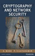
Find the result of 2320 mod 29.
Table 2.1 shows the result of this problem. In this table, first column uses exponent y as the exponent value. The second column partial result (PR) indicates that it holds (PR). The third column is used to indicate the final result by performing a modulo division operation with respect to PR. In this table, initially we consider the exponent value as 2, for which PR and PR mod 29 values are computed. After that, we have to take the exponent value as 3 for which the output of the previous exponent value is given as the input. Therefore, the output of nth round is given as the input value to (n + 1)th round when calculating PR value. Therefore, this algorithm works faster than the previous exponentiation algorithm.
Table 2.1 Working example of memory-efficient algorithm
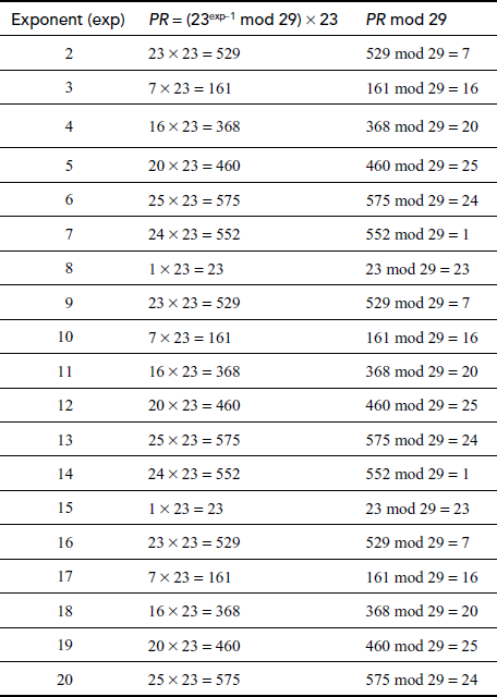
This method of computing modular exponentiations can be formalized into an algorithm as shown in Algorithm 2.1.
Here, the value x is the base which is greater than 1, y is the exponent value and n is the modulo value.
Fast Modular Exponentiation Algorithm
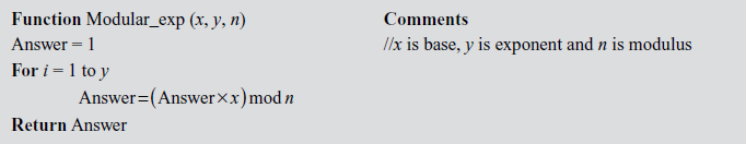
Fast modular exponentiation is an algorithm which is used to reduce the computation complexity further. The main advantage of this algorithm is that the execution time of this algorithm is O(log y)1 where y is the exponent value. The main idea of this method is that the exponent value y is represented in the form of binary bits. For example, if the exponent value y is 8, then this will be represented as y = 8 = 1000. This method of computing modular exponentiations can be formalized into an algorithm as given in Algorithm 2.2.
In this algorithm, the exponent y is converted into binary bits by performing a modulo division operation (y mod 2). If the result of this modulo division operation is 1, then it will multiply the base value x with Answer and the result is modulo divided with n ((Answer × x) mod n). If the result is not equal to 1, then a 1-bit right shift operation is performed followed by squaring operation with respect to the base value x. Therefore, the fast exponentiation algorithm performs both multiplication and squaring operation.
Example 2.8:
Find the result of 5117 mod 19.
Step 1: Divide the exponent 117 into powers of 2 in order to convert them into binary format.
i.e., 
After converting it to binary format, start to read from the rightmost digit. Initially, take k = 0 and for each digit add 1 to k, and move left to take the next digit. If the digit is 1, we need to include a part for 2k, otherwise do not include that position.


Step 2: Calculate mod n of the powers of two 1 y


Step 3: Use modular multiplication properties to combine the calculated mod n values


Therefore, 
2.1.4 Greatest Common Divisor Computation
The greatest common divisor (GCD) of two or more integers is defined as the greatest positive integer that divides the numbers without a remainder. It is also called the highest common divisor (HCD), or highest common factor (HCF). For example, the GCD of 18 and 30 is 6. Because the integer 18 can be divided by {2, 3, 6, 9} and the integer 30 can be divided by {2, 3, 5, 6, 10, 15}. The greatest number that divides these two numbers is 6. If the GCD of any two numbers is 1, then these two numbers are relatively prime number or co-prime. For example, the GCD of (12, 13) = 1 and hence they are co-primes. When the given numbers are too larger numbers, for example, 512 bits or 1024 bits, then listing of all the divisors of the given numbers is a complicated task. Therefore, we have to use a computationally efficient method for computing the GCD value of large numbers. The GCDs can be computed by using various computationally efficient methods, namely prime factorizations, Euclid’s algorithm and extended Euclid’s algorithm.
2.1.4.1 Prime Factorizations
To compute GCD of any two numbers in prime factorization approach, we need to find prime factors of the two numbers. The prime factorization is also a method used in factoring algorithms. Prime factors of any number can be computed by dividing that number by all prime numbers starting from  that exactly divides that number without giving remainder number. The following is an example for computing prime factors of a given number.
Example 2.9:
Find the prime factors of the number 7007
Step 1: Divide the given number 7007 by all prime numbers that produces an integer number.
Hence, the prime numbers 2, 3 and 5 cannot divide the given number exactly. So,  11an integer number.
However, the prime numbers 7, 11 and 13 exactly divide the number 7007.
Hence, 
Therefore, 

After computing the prime factors, the prime factors are used in computing the GCD value by taking the common prime factors of the given two numbers. For example, to compute the GCD value of (78,120) we need to find the prime factors of (78, 120). In order to compute GCD value, the prime factors are computed in the initial step. To compute the prime factors, we can use the prime factorization method as explained in Example 2.9. The prime factors of these two numbers are given below:

 .
.
From the results of the prime factors of these two numbers, it is clear to see that 2 × 3 is common in both the numbers. Therefore, the GCD value of (78,120) = 2 × 3 = 6. The main limitation of this method is that it is only feasible for small numbers since computing prime factorizations takes more running time. Moreover, a listing of all the prime factors of the given two numbers also takes more running time.
Euclid’s Algorithm
It was developed by the great Greek mathematician Euclid who was popularly referred to as the ‘Father of Geometry’ in about 300 BC for computing the GCD of two positive integers. It is a more efficient method than the prime factorization method that uses a division algorithm in combination with the observation that, the GCD of two numbers also divides their difference. The Euclid’s algorithm is given in Algorithm 2.3.
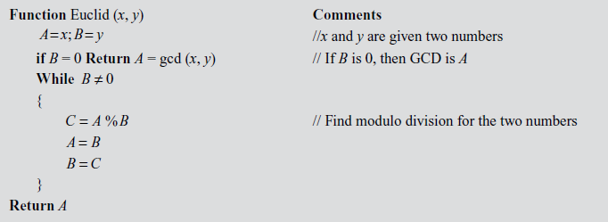
It is clear from the description of the Euclidean algorithm that if any one of the values is zero for the given two values, then GCD value is the other non-zero value. For example, if B = 0, then the algorithm returns A value is the GCD value (A = gcd(x, y)). Otherwise, divide the A value by the value of B and store the remainder value in the variable C. After that, a swapping operation is performed by assigning the value of B to A and C to B. This operation is repeated until B = 0.
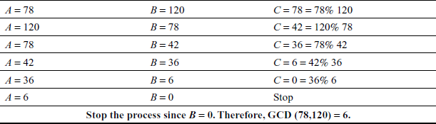
Example 2.10:
Find the GCD of (78, 120) using Euclid’s Algorithm
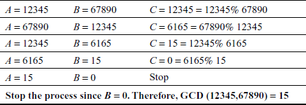
Example 2.11:
Find the GCD of (12345,67890) using Euclid’s Algorithm
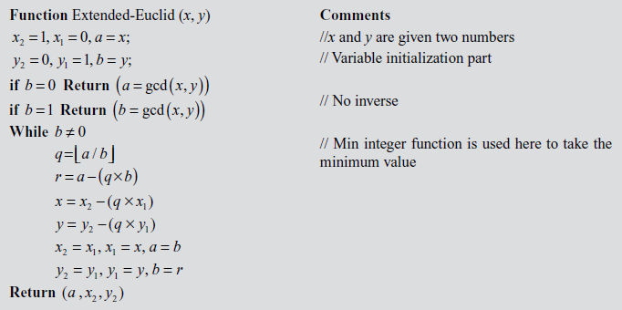
Extended Euclidean Algorithm
Extended Euclidean Algorithm is an efficient method of finding the modular inverse of an integer. Euclid’s algorithm can be extended to give not only d = gcd(a, b), but also used to find two numbers x2 and y2 such that  . What is the use of these extra numbers? Suppose we want to check whether our gcd program is correct and to check the correctness of the answer. One easy test is to simply check whether d divides a and d divides b. Clearly this is not a sufficient test since it only verifies that d is a common factor, not that it is the GCD value. In order to check d is the GCD value of a and b, we have to check two conditions. Firstly, we have to check whether d divides a and d divides b. Secondly, we have to check
  . If d satisfies these two conditions, then d is the GCD value of a and b. Algorithm 2.4 explains about the extended Euclidean algorithm. In this algorithm, the input numbers x and y are copied into a temporary variable and are treated as
  . In each trial, r value is computed to swap the contents of the initial values of a and b. Similarly, x and y values are computed by using
  and
and  . These values are used to update the values x2 and y2 by performing a swapping operation. The same process is repeated until b ≠ 0 and finally the algorithm returns the values
  as output. From the returned value, the value a is considered as d.
Example 2.12:
Find the GCD of (4864, 3458) using extended Euclid’s algorithm.
Solution
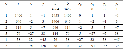
We get gcd(a, b)11gcd(4864, 3458) = 38. Because 38 divides both the numbers (4864, 3458), it satisfies the first condition. The answer can also be verified by using the equation (a × x2) + (b × y2) = d. Substitute the values, a = 4864, b = 3458, x2= 32 and y2= –45 in the equation (a × x2) + (b × y2) = (4864 × 32) + (3458 × (–45))1 
Therefore,  since it satisfies both the conditions.
Example 2.13:
Find the GCD of (9,437) using extended Euclid’s algorithm.
Solution
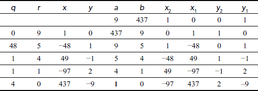
We get gcd(a, b) = gcd(9,437) = 1. Because 1 is the one and only number that divides both the numbers (9,437), it satisfies the first condition. The answer can also be verified by using the equation (a × x2) + (b × y2) = d. Substitute the values, a = 9, b = 437, x2 = –97 and y2 = –2 in the equation (a × x2) + (b × y2) = (9 × (–97)) + (437 × (2)) 
Therefore, gcd(9,437) = 1 since it satisfies both the conditions. In this case, the input numbers are said to be co-primes.
Example 2.14:
Find the GCD of (9,195) using extended Euclid’s algorithm.
Solution
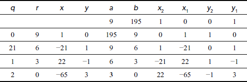
We get gcd(a, b)11gcd(9,195) = 3. The answer can be verified by using the equation (a × x2) + (b × y2) = d. Substitute the values, a = 9, b = 195, x2 = 22 and y2 = –1 in the equation (a × x2) + (b × y2) = (9 × 22) + (195 × (–1)) 

Therefore, 
Example 2.15:
Find the GCD of (9,195) using Extended Euclid’s Algorithm.
Solution
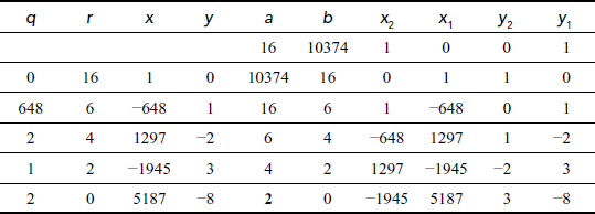
We get gcd(a, b)11gcd(16,10374) = 2. The answer can be verified by using the equation (a × x2) + (b × y2) = d. Substitute the values, a = 16, b = 10374, x2 = –1945 and y2 = 3 in the equation (a × x2) + (b × y2) = (16 × (–1945)) + (10374 × (3))
Therefore, 
2.2 Chinese Remainder Theorem
Let us assume that  are pairwise relative prime positive numbers, and that
  are positive integers. Then, Chinese remainder theorem (CRT) states that the pair of congruences,


has a unique solution mod  . To compute the unique solution, we need to compute the value as shown in Equation (1).
 (1)
(1)
where  and
and 
CRT is used to find a common value from a system of congruences. For example, some quantity of mangos are available in a room. If the mangos are divided into groups consisting of three mangos in each group, then remaining two mangos are available. Similarly, if the mangos are divided into groups consisting of five mangos in each group, then remaining of three mangos are available. If the mangos are divided into groups consisting of seven mangos in each group, then remaining of two mangos are available. Finally, how many mangos are available in total in that room? For computing the answer to this puzzle, there are two approaches, namely trial-and-error-based approach (brute force method) and CRT-based approach. In brute force method, first we have to generate the system of congruences from the given puzzle. The first congruential equation that can be formed for the first constraint is X ≡ 2(mod 3), where X is the amount of mangos, 2 is the remainder, and 3 is the group size. Similarly, other congruential equations that can be formed by using the same way. The remaining two congruential equations for the remaining two constraints are X ≡ 3(mod 5) and X ≡ 2(mod 7).
For computing the total amount of mangos by using the brute force method, we have to find the value of X that satisfies first congruential equation. Next, we have to find the value of X that satisfies second congruential equation. Similarly, we have to find the value of X that satisfies third congruential equation. Finally, we have to find the intersection of the three sets to get the value of X that satisfies all the three congruences. The values of X that satisfies all the three congruences are given in three different sets.


The intersection of these three sets is 23. One of the limitations of this approach is that, it is useful when the values of ai and ki are small. For slightly larger numbers, making this list is a complex task and also it would be an inefficient approach. Therefore, CRT is the suitable method for large numbers in order to compute the value of X. Example 2.16 uses the CRT approach for solving the above problem.
Example 2.16:
Find the value of X from the system of congruences.
X ≡ 2(mod 3)
X ≡ 3(mod 5)
X ≡ 2(mod 7)
Solution
Let, 

Find the multiplicative inverse element of M1, M2 and M3.
Let y1 be the inverse element of1M1.
- 2 is an inverse element of M1 because

#9; Because,

- 1 is an inverse element of

- 1 is an inverse element of

Therefore, 


Example 2.17:
Find the X value using the CRT for the following:
X ≡ 3(mod 5)
X ≡ 4(mod 6)
X ≡ 5(mod 7)1
Solution
 1
1


Let y1 be the inverse element of M1 and to find y1 we have to use the following equation: M1y1 ≡ 1mod k1

If we substitute y1 value as 3, it will satisfy the condition  . Because,
  Hence,
Similarly, (35 × y2) ≡ (35 × 5) ≡ 1 mod 2. y2 = 5
y3 = 4. Because, (30 1 4)mod 7 = 1
To find the value of X:


 1
1
 1
1
CRT is mainly used in coding theory and cryptography. In coding theory, CRT is mainly used for detecting and correcting the errors occurred in the data by adding some redundant bits to the original data when the data is communicated through noisy channels. In cryptography, CRT is used for sharing a common secret value (key value) to a group of users called key distribution. Section 2.2.1 explains the method of distributing a common group key value to a group of users through secure multicasting key distribution using CRT.
2.2.1 Secure Multicasting using CRT
In multicast communication, messages are sent from one sender to a group of members. Multicast group formation and group communication are very common in the Internet scenario. This is helpful for sending and exchanging private messages among group members. Moreover, multimedia services such as pay-per-view, video conferences, sporting events, audio and video broadcasting are based on multicast communication where multimedia data are sent to a group of members. In order to form groups and to control the activities of a group, a leader in the group is necessary. In most of the multimedia group communication, a group centre (GC) or key server (KS) is responsible for interacting with the group members and also to control them. In such a scenario, groups can be classified into static and dynamic groups. In static groups, membership of the group is predetermined and does not change during the communication. Therefore, the static approach distributes an unchanged group key to the members of the group when they join or leave from the multicast group. Moreover, they do not provide necessary solutions for changing the group key when the group membership changes which is not providing forward/backward secrecy. When a new member joins into the service, it is the responsibility of the KS to prevent new members from having access to previous data. This provides backward secrecy, in a secure multimedia communication. Similarly, when an existing group member leaves from any group, the GC should not allow the member to access the future multicast communication which provides forward secrecy. The backward and forward secrecy can be achieved only through the use of dynamic group key management schemes. In order to provide forward and backward secrecy, the keys are frequently updated whenever a member joins or leaves the multicast service.
In secure multicast communication using CRT, the KS initially selects a large prime number p1and q, where p > q and  . The value p helps in defining a multiplicative group z*p and q is used to fix a threshold value to select the group key values. To understand the clear idea of multiplicative group z*p, we request the readers to refer Section 2.4.1 before reading this topic. Initially, the KS selects secret keys or private keys ki from the multiplicative group z*p for n number of users which will be given to users as they join into the multicast group. In the CRT-based scheme, we require that all the private keys selected from z*p are pairwise relatively prime positive integers. Moreover, all the private keys should be much larger than the group key which is selected within the threshold value fixed by q. Next, KS executes the following steps in the KS initialization phase.
- Compute

- Compute

- Compute yi such that

- Multiply all users xi and yi values and store them in the variables,

- Compute the value

User Initial Join
Whenever a new user ui is authorized to join the dynamic multicast group for the first time, the KS sends a secret key ki using a secure unicast which is known only to the user ui and KS. Next, KS computes the group key in the following way and broadcasts it to the users of the multicast group.
(a) Initially, KS selects a random element kg as a new group key within the range q.
(b) Multiply the newly generated group key with the value μ (computed in KS Initial set-up phase).

(c) The KS broadcasts a single message to the multicast group members. Upon receiving
  value from the KS, an authorized user ui of the current group can obtain the new group key kg by doing only one mod operation.
 1
1
The kg obtained in this way must be equal to the kg generated in step a) of user initial join phase. When i reaches n, KS executes its initial set-up phase to compute  for m number of users, where 1for m number of users, where 1 is a constant value which may take values less than 5 depending upon the dynamic nature of the multicast group.
User Leave
Group key updating operation when a user leaves usually takes more computation time in most of the group key management protocol since the KS cannot use the old group key to encrypt the new group key value. When a new user joins the service, it is easy to communicate the new group key with the help of the old group key. Since the old group key is not known to the new user, the newly joining user cannot view the past communications. This provides backward secrecy. User leave operation is completely different from user join operation. In user leave operation, when a user leaves the group, the KS must avoid the use of an old group key to encrypt a new group key. Since the old user knows the old group key, it is necessary to use each user’s secret key to perform a re-keying operation when a user departs from the services. In this key management scheme, the group key updating process is performed in a simplest way. When a user ui leaves from the multicast group, KS has to perform the following steps.
- Subtract vari from
 .
. 
- Next, KS must select a new group key and it should be multiplied with
 to form the rekeying message as shown below.

- The updated group key value will be sent as a broadcast message to all the existing group members. The existing members of the multicast group can get the updated group key value k′g by doing only one mod operation as shown in step (c) of user initial join process. From the received value, the user ui cannot find the newly updated group key k′g since his or her component is not included in
 .
.
2.2.2 Implementation of CRT in JAVA
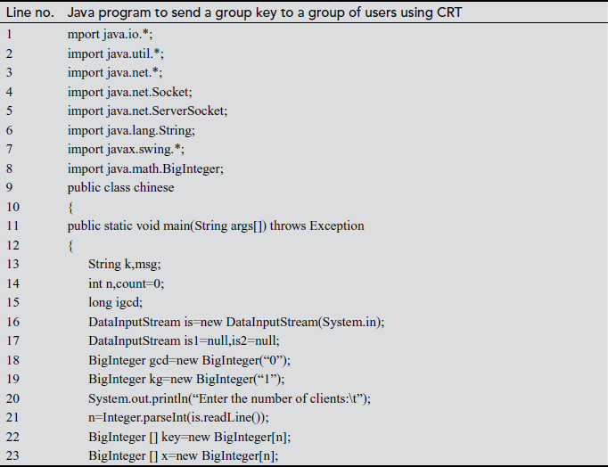
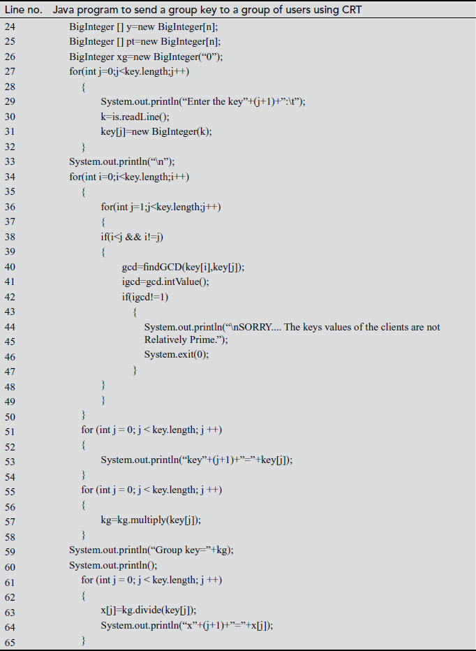
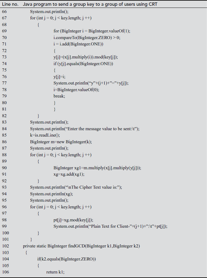
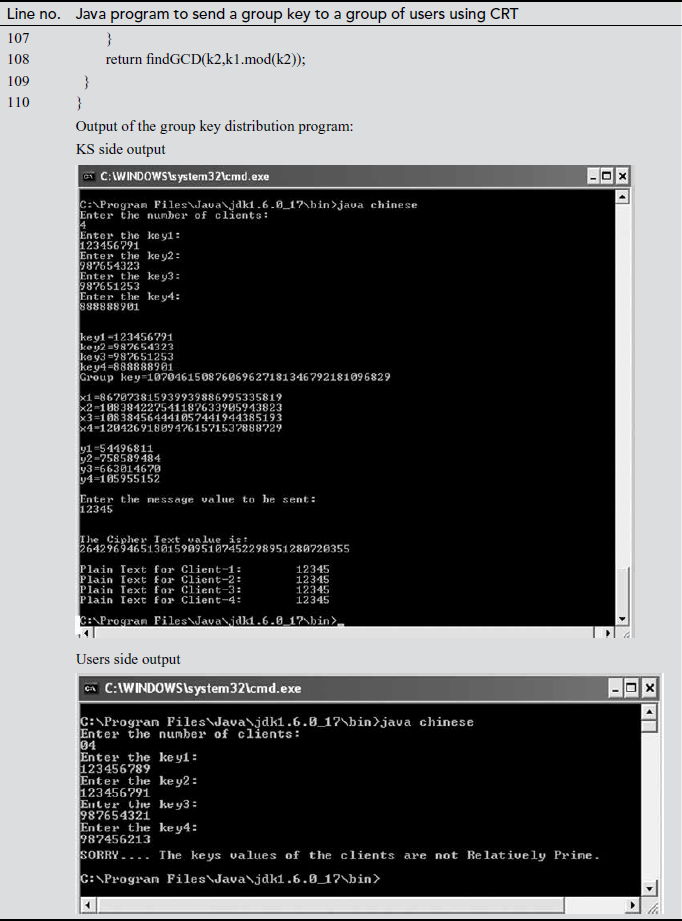
In the above program, line numbers 27 to 32 are used to generate user’s private key at KS side. These private keys are informed to each user in a secure way in real-time applications. Line numbers 34 to 49 are used to check whether these numbers are relatively prime numbers. Because in CRT, one of the important conditions is that all users private keys are relatively prime numbers. In line number 57, each user’s private key is multiplied by using the method ‘multiply’ and is stored in a variable ‘kg’. The statements used from line numbers 61 to 65 are used to find the xi values of each user. Line number 73 is used to find the yi values of each user. The xi values and yi values are multiplied and are stored in the variable ‘xg1’. In line number 91, the group key value to be communicated to a group of users is added to the variable ‘xg1’. Each user group can perform only one modulo division operation to take the group key by using the method ‘mod’ as given in line number 98.
2.3 Fermat’s and Euler’s Theorem
Pierre de Fermat is a mathematician who stated this theorem in the year 1640.
Fermat’s Theorem
If p is a prime and p does not divide a which is a natural number, then  .
.
For example,  since 11 is a prime number and 11 does not divide 2. The Fermat’s theorem is mainly used to solve modular exoneration problems when the base is considered as a, moduli are considered as prime p and p should not divide a. It is also called Fermat’s little theorem or Fermat’s primality test and is a necessary but not a sufficient test for primality test. Primality test is a method which is used to test whether a whole number is a probable prime or not. These numbers are very important and are used in many cryptographic algorithms.
Example 2.18:
Compute the value of 210 mod 11.
(210) ≡ 1 mod 11. Therefore, the result is 1.
Example 2.19:
Compute the value of 2340 mod 11.


Example 2.20:
Compute the value of 412345 mod 12343
 ≡
≡ 
Fermat’s Theorem 1:
If p is a prime and p does not divide a, then ap ≡ a mod p
Fermat’s Theorem 2:
If p is a prime and p does not divide a, then ap–2 mod p ≡ a–1 mod p
Euler’s Theorem
If n and a are co-prime positive integers, then  . In this theorem,
  if n is a prime number and
  is Euler’s phi function. Euler’s phi function is also called Euler’s totient function and hence it is named as Euler’s totient theorem or Euler’s theorem.
Euler’s phi function  (n):
(n):
Euler’s phi function  returns the number of integers from 1 to n, that are relatively prime to n. The phi function
  is computed using various methods. They are given below.
- If n is a prime number, then
 .
. - If n is a composite number, then
2.1 Find the prime factors of that number and compute the phi function value as used in step 1. Otherwise,
2.2 Find prime powers (pa) of the given number n. For computing the phi value of prime powers we have to use the formula
 .
.
Example 2.21:
Compute Euler’s totient function for the values 3, 8, 12, 60, and 7007.


Example 2.22:
Compute Euler’s totient value of 17640.


Euler’s theorem uses modulo arithmetic and is an important key to RSA encryption and decryption. The following Java program explains the use of Euler’s totient function for multicast key distribution.
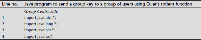
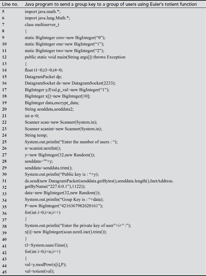
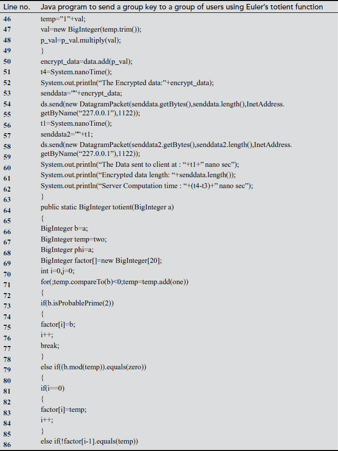
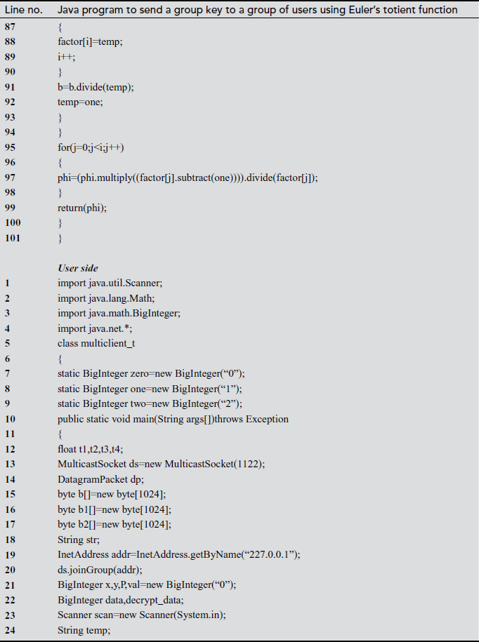
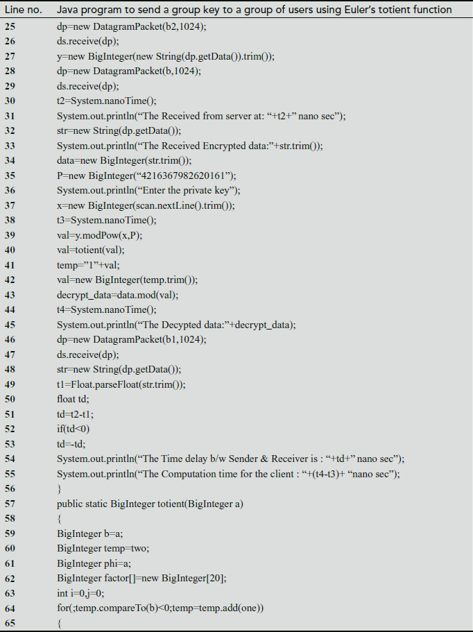
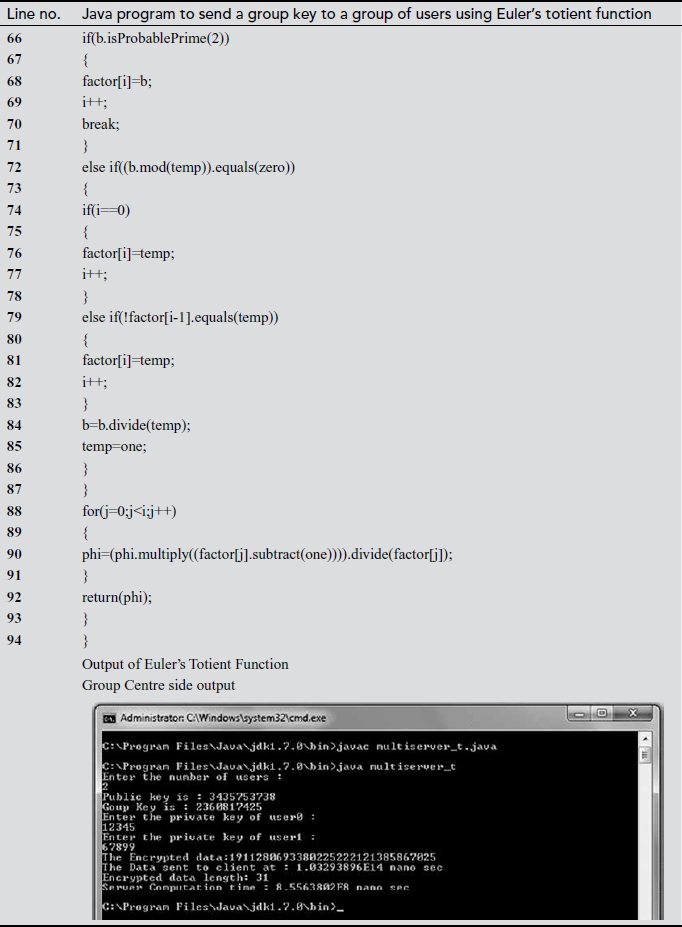
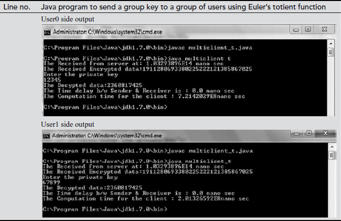
In the above program, there are two programs, namely GC side and user side programs. The main use of this program is to send a common group key to a group of users. The key distribution module used in the GC side and key updating module used in the user side both uses Euler’s totient function. In the GC side program, the line numbers 42 to 49 are used to generate a common group key. During the group key computation, in line number 45 Euler’s totient value is computed and the result is stored in a temporary variable ‘val’. For computing the totient value, we define a function ‘totient (val)’ in both the GC and user side program. The totient function is implemented from line numbers 64 to 101. After computing the group key value, the group key is encrypted in line number 50. The encrypted group key is sent to a group of users in the GC side from line number 54 to 55. On the user’s side, the encrypted key value is received in line number 26. The received encrypted group key value is decrypted in the user side in line number 43.
2.4 Algebraic Structure
An arbitrary set with one or more limited operation defined on it with certain axioms is called an algebraic structure. There are three types of algebraic structures, namely groups, rings and fields. Various operations performed on these algebraic structures are addition, subtraction, multiplication and division operations. Each operation takes any two elements from the defined algebraic structure as input and produces a third element as output which will also be available in the algebraic structure. For example, a1and b are the two input values taken from any one of the algebraic structures. The input values can be added to produce an output element c by using commutative law (i.e. a + b = c). According to the principles used in algebraic structure, the resultant element c will also be available in the algebraic structure from where the input values are taken. The complex algebraic structures are vector spaces, modules and algebras where multiple operations can be performed. Algebraic structures are mainly used in various cryptography algorithms to process with integer numbers. Figure 2.1 shows the classification of algebraic structures and the operations supported by each algebraic structure.
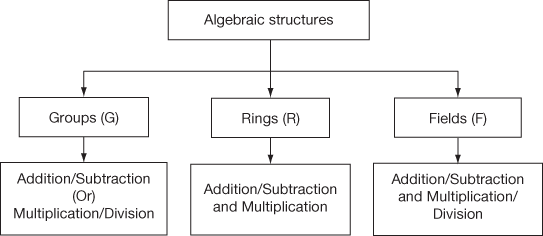
Figure 2.1 Types of algebraic structures and their binary operations
The group supports addition/subtraction operation or multiplication/division operation. But it is not supporting both the addition and multiplication operations. There are two types of groups used in cryptographic algorithms, namely additive group and multiplicative group. If the group supports addition operation in the encryption function and subtraction operation in the decryption function, then it is called an additive group. If the group supports multiplication operation in the encryption function and division operation in the decryption function, then it is called a multiplicative group. Ring supports addition/subtraction operation and also it supports the multiplication operation. Therefore, the ring supports two operations at a time. Field is the combination of the group and ring and it supports all the four types of binary operations such as addition, subtraction, multiplication and division operations. The following subsections explain about all the algebraic structures in detail.
2.4.1 Group
A group contains a set of elements denoted as G together with a binary operator * on G that satisfies the following axioms:
- Closure
If
 , then
  also belongs to G.
 - Associative

- There exists an identity element
 with the property that

- For each element
 , there exists an inverse element

The binary operation * in this definition may be any operation such as addition, subtraction, multiplication and division. Any group of elements with an operation that satisfies these four axioms forms a group. For example, the set of integers  forms a group under the operation of addition. In particular, when addition operation is used in a group it is called an additive group. In the additive group, the element 0 is an additive identity, and every integer has an additive inverse. For multiplicative group, a multiplication operation is used. In multiplicative group, the element 1 is used as a multiplicative identity and every integer of that group has a multiplicative inverse. For example, the set of non-zero real numbers
  forms a group under the operation of multiplication. The group is an important algebraic structure used in many cryptographic algorithms. If a developer wants to develop a new encryption function that uses an addition operation, then an additive group can be used for that encryption function. If the encryption uses a multiplication operation in the encryption function used on the sender side and division operation to use it in the decryption function used on the receiver side, a multiplicative group can be used.
Groups can also be divided into two types, namely finite groups and infinite groups. The finite groups use a finite number of elements and it has a limit, for example n where n is a finite number. In infinite groups, the group can take an infinite number of elements starting from 0 to ∞. Most of the cryptographic algorithm uses finite groups. Therefore, this bookwork mainly focuses on discussing about finite groups by using a finite set of numbers.
Example 2.23:
Consider the group  where
where  . Prove that the given group is an additive group.
Solution
Since n = 10, the group can have 10 elements. That is,  . To prove that the given group is an additive group, we have to check whether it satisfies the following four axioms:
- Closure: Take a = 4, b = 9 ∈ G, then a +n b = 3, which is also available in the group G and hence it satisfies the first axiom. (The symbol +n denotes addition modulo operation where a modulo division operation is performed after performing an addition operation with respect to n = 10.)
- Associative:
 . To prove the associative property, consider
  . If we substitute these values in associative property, it will give the following result.
L.H.S =

R.H.S

LHS = RHS and hence it satisfies the associative property also.
- There exists an identity element
 because

- For each element
 , there exists an inverse element
  . Take any element from Figure 2.2, for example, 4 which has the additive inverse 6 because
  .
.
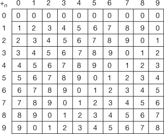
Figure 2.2 Addition modulo 10
Therefore, the given group is an additive group because it satisfies all the four axioms of an additive group.
Example 2.24:
Consider the group  , where
 . Prove that the given group is a multiplicative group.
Solution
Since  , the group can have 10 elements. That is,
  . To prove that the given group is a multiplicative group, it should satisfy the following four axioms for non-zero elements to form a multiplicative group.
- Closure: Take
 , then
  which is also available in the group G and hence it satisfies the first axiom.
 - Associative: a (b × c) = (a × b) × c. To prove the associative property, consider a = 4, b = 9, c = 6 ∈ G. If we substitute these values in associative property, it will give the following result.
LHS =

RHS

LHS = RHS and hence it satisfies the associative property also.
- The identity element 1 ∈ G does not exist for any of the non-zero elements of the group. For example, the identity element is not generated in Figure 2.3 for the elements
 .
. - For some of the non-zero elements, there is no existence of a multiplicative inverse element
 . For example, multiplicative inverse is not generated for the elements
  from Figure 2.3.
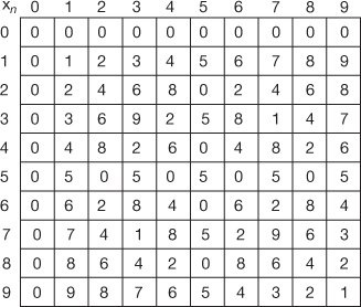
Figure 2.3 Multiplication modulo 10
Therefore, the given group is not a multiplicative group because it does not satisfy the last two axioms to form a multiplicative group.
In the above example, the elements  are not producing multiplicative inverse because when any one of these elements is multiplied with another element and a modulo division operation is performed with respect to size of the group, it is not giving the result as 1. For example,
  where
where  is any element of the given group
  . In most of the cryptographic algorithms where a multiplication operation used in the encryption function, it should generate multiplicative inverse for all the elements of the group. If this condition is not satisfied, then the output value produced by the decryption function will not be equal to the input value supplied to the encryption function.
Consider, for example, we want to design an encryption and decryption function to be used in any one of the security-oriented applications. The encryption function is (x × y = z) and the decryption function is  where x is the plaintext, y is the key value selected from a multiplicative group and z is the ciphertext. To make further discussion about this concept, consider the multiplicative group
  where n = 10 used in the above example. By using this multiplicative group, we shall do the encryption and decryption operation for the plaintext value x = 8 and the key value y = 5.
Encryption:

Decryption:

Therefore, the decryption function is not producing the actual plaintext which was given as the input in the encryption function. The main reason is that the given group is not a multiplicative group and hence it is not suitable for the cryptographic algorithms where multiplication operation is used in the encryption function and division operation is used in decryption function. Therefore, this type of additive group is suitable for the cryptographic algorithms where addition operation is used in the encryption function and subtraction operation is used in the decryption function (for example, Caesar cipher or shift cipher). In order to use multiplication operation in the encryption function side, we need to change the group in such a way that all the elements of the group should produce multiplicative inverse. For example, if the group  is changed as
  , then all the elements of the group will produce multiplicative inverse.
The reason is that all the elements are relatively prime to order or size of the group 7. This type of group is called a prime group and is denoted as  . The prime group is used in many cryptographic algorithms such as Diffie–Hellman and Elgamal cryptosystem, etc. Figure 2.4 shows an example of a prime group. It is very clear to see from Figure 2.4(b)) that all non-zero elements produce multiplicative inverse and hence it forms a multiplicative group.
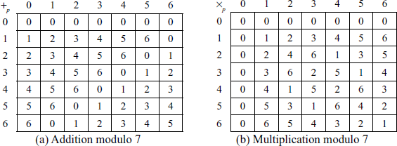
Figure 2.4 Addition and multiplication operation performed on a prime group
2.4.2 Ring
A ring R is a set of elements together with two binary operations addition (+) and multiplication (×) operations that satisfies the following axioms:
- If a, b ∈ R, then the sum (a + b) and the product (a × b) also belong to R.
- The addition operation is associative. That is,
 , where,
  .
. - There exists an additive identity, denoted by the symbol 0. This element has the property that a + 0 = a, where a ∈ R.
- For each element a ∈ F, there is an element − a ∈ R, called the additive inverse of a, with the property that a + (–a) = 0.
- The addition operation is commutative. That is,
 where
where .
. - The multiplication operation is associative. That is,
 where
where  .
. - There exists a multiplicative identity, denoted by the symbol 1. This element has the property that
 where
where  .
. - For each element
 other than 0, there exists an element
  , called the multiplicative inverse of a, with the property that
  .
. - The multiplication operation distributes over the addition operation. That is,
 where
where .
.
A ring R is an Abelian group with respect to addition operation for the first four axioms. A ring which satisfies commutative property is called a commutative ring. If the ring R satisfies eighth axiom, then it is called a division ring. If the ring R is a commutative and division ring, then it is called a field. Figure 2.4 is an example of a ring and a field.
2.4.3 Field
A field F is a set of elements together with two binary operations addition (+) and multiplication (×) operation that satisfies the following axioms:
- If
 , then the sum (a + b) and the product (a × b) also belong to F.
 - The addition operation is associative. That is,
 , where
  .
. - The addition operation is commutative. That is,
 where
where  .
. - There exists an additive identity, denoted by the symbol 0. This element has the property that a + 0 = a, where a ∈ F.
- For each element a ∈ F, there is an element − a ∈ F, called the additive inverse of a, with the property that a + (–a) = 0.
- The multiplication operation is associative. That is,
 where
where  .
. - The multiplication operation is commutative. That is,
 where
where  .
. - There exists a multiplicative identity, denoted by the symbol 1. This element has the property that a × 1 = a, where a ∈ F.
- For each element a ∈ F other than 0, there exists an element a–1 ∈ F, called the multiplicative inverse of a, with the property that a × (a–1) = 1.
- The multiplication operation distributes over the addition operation. That is, a × (b + c) = (a × b) + (a × c), where a, b, c ∈ F.
Example 2.25:
What is the value of x from the equation 3x + 4 ≡ 6(mod 7)?
Solution
Since 7 is used in the modulo division operation, it is considered as  which is a finite field. The order of the field is 7. In order to solve this equation using elementary algebra, first we subtract 4 from both sides and get the result as given below:

From this, the value of x can be found by,
 .
.
The multiplicative inverse of the element 3 in  is
is  which is taken from Figure 2.4(b)). It can also be computed by using the direct method as shown below:


The value 3 is multiplied with the entire elements of the field and a modulo division operation is performed with respect to the order of the field. If the result becomes 1 for any of the operations, stop at this point and consider that element as a multiplicative inverse. In this case, the element 5 becomes a multiplicative inverse of 3 because . Substitute the value 5 in the place where
  is used.
This gives,  .
.

Therefore,  .
.
The field (F) is divided into two types, namely a finite field and an infinite field. Finite field is mainly used in cryptography to design a computationally efficient algorithm. Finite field is also called a Galois field (GF) that has a different structure than field structure. GF is used in many cryptographic algorithms such as advanced encryption standard (AES) and elliptic curve cryptography (ECC). The order, or number of elements, of a finite field is represented in the form of (pn), where p is a prime number and n is a positive integer. For every prime number p and positive integer n, there exists a finite field with (pn)1elements. Another notation for a finite field is of the form GF(pn), where the GF represents a ‘Galois Field’. One important issue in the structure (pn) is that arithmetic operations modulo (pn) do not satisfy all the axioms of a field. Consider, for example, p = 2 and n = 8 and then the field will have the set of integers from 0 to 63. Therefore, the field will have 64 integer elements and the order of the field is 64. Since 64 is not a prime number, the set of integers is not a field. In order to make it to become a field, we have to choose a closest prime number to the size of field 64. The closest prime number of the order of the field 64 is 61. However, in this case the numbers 61, 62 and 63 are not used in the field and hence it is an inefficient way of using a field. Therefore, the GF is purely based on polynomial equations. Hence, it is necessary to discuss about polynomial arithmetic before proceeding of GF in this section. To add any two polynomials, the terms must be combined. For instance, the addition of two polynomial equations 3x and 5x can be 8x by adding its terms. Likewise, 3x2y and 5x2y can be added to get 8x2y. However, 3x2y and 5x2y3 cannot be added together. The reason is that these two terms do not have the exact variables and the exact powers of those variables. The basic definitions used in polynomial equations are given below:
- Polynomial: A polynomial in x is any expression which can be written as:

where
 are integers and an ≠ 0
 - Degree: The degree of a polynomial is the highest exponent of the polynomial.
- Monomial: It is a polynomial with one term.
- Binomial: It is a polynomial with two terms.
- Trinomial: It is a polynomial with three terms.
- Like terms: It means the same variable to the same power. For example, 2x2 and 3x21are like terms because they have the same variable raised to the same power. However, 2x2 and 3x3 are not like terms because the powers are different.
Example 2.26:
Add the two polynomial equations  and
and  .
.
Solution

Example 2.27:
Subtract the two polynomial equations  and
and  .
.
Solution

Example 2.28:
Multiply the two polynomial equations  and
and  .
.
Solution
To multiply polynomials, multiply each term in the first polynomial by each term in the second polynomial. In order to do this, we need to recall the product rule for exponents: For any integers 


In polynomial division, there are two types of polynomial division, namely simplification method and real division method. If there is a common factor both in the numerator (top) and denominator (bottom), then simplification method is used. Otherwise, real polynomial division is used. For example, divide the polynomial 2x + 4 by using the constant polynomial 2. Here, we can use a simplified method because there is a common factor 2 both in the numerator and denominator. Therefore,  .
.
Example 2.29:
Divide the polynomial 21x3 – 35x2 by using 7x.
Solution


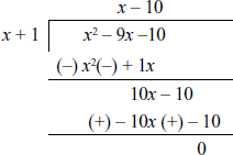
Example 2.30:
Divide the polynomial x2 – 9x – 10 by x + 1.
Solution
2.4.4 Galois Fields
This subsection discusses about the way of performing arithmetic operations in the structure GF(pn). The addition and subtraction operations are performed by adding or subtracting two polynomials together, and reducing the result modulo the attribute p. In a finite field with the attribute p = 2, addition modulo 2 is performed for addition operation and subtraction modulo 2 is performed for subtraction operation. This is very identical to performing XOR operation. Therefore, simple XOR operation can be used for performing addition and subtraction operations when p = 2 in the Galois field GF(2n). For example, addition/subtraction of given two polynomials f(x) = x2 + 1 and g(x) = x2 + x +1 taken from GF(23) is x.
Multiplication operation in a Galois field GF(2n) is performed by multiplication modulo an irreducible reducing polynomial used to define the Galois field GF(2n). During the multiplication operation performed in GF, a multiplication operation followed by a modulo division operation is performed using the irreducible polynomial as the divisor. Irreducible polynomial m(x) is a polynomial that has no divisors other than itself and 1; otherwise, it is called a reducible polynomial. A few examples of some irreducible polynomials of GF(2n) are  ,
,  ,
, 
 ,
,  . A few examples of reducible polynomials are
  ,
,  , and (x3 + x2). Irreducible polynomial is used in GF(2n) because reducible polynomials are not generating the multiplicative inverse for any of the elements of GF(2n). Therefore, it is necessary to choose an irreducible polynomial in the cryptographic algorithms where multiplication operation is used in the encryption function and division operation is used in the decryption function. For example, multiply the given two polynomials f(x) = x2 + x and g(x) = x2 taken from the Galois field GF(23) for the irreducible polynomial m(x) = x3 + x2 + 1.

 (since
 =
=
 =
=  )
)
=  (since
  )
)
=  (since
 =
=
 =
=
=  1
1
= 1 (substitute
  value as
  =
= 
Table 2.2 Polynomial arithmetic modulo (x3 + x2 + 1)
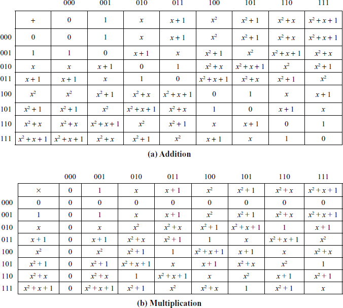
The arithmetic operations performed in GF (23) for the irreducible polynomial (x3 + x2 + 1) is shown in Table 2.2. Similar to the arithmetic operations performed in the algebraic structure GF(2k) which was discussed before, the Galois field GF(3k) uses the same way of performing the arithmetic operations with some changes are included. For example, the addition/subtraction is treated as performing an XOR operation in GF(2k). However, the addition/subtraction operation is performed in a different way in GF(3k). Because, it has three coefficients {0, 1, 2} and hence it is represented as  . The irreducible polynomials of GF(32) are x2 + 1, x2 + 2, x2 + x + 1, x2 + x + 2, x2 + 2x + 1, and x2 + 2x + 2. To construct GF(3k) with any one of the irreducible polynomials, a set of elements with the degree of at most (k - 1) is used in the set. For example, GF(32) has group of 9 elements and they are of the form a1x + a0, where
  These 9 elements are given as {0, 1, 2, x, x + 1, x + 2, 2x, 2x + 1, 2x + 2}. Consider the polynomial equations
  chosen from GF(32). The addition of these polynomial equations can be performed in the following way:

 (Since, 3 mod 3 is zero)
Similarly, all the elements of the group can be added. In order to perform multiplication in GF(32), an irreducible polynomial of degree 222over GF(3) is required. This polynomial will be in the form of x2 + ax + b such that  . Therefore, we choose the irreducible polynomial x2 + 2x + 2 for our discussion.
Note:
It is to be noted that  (Otherwise, the polynomial would be x2 + ax which is a reducible polynomial.)
To perform multiplication operation in GF(32) for the elements f(x) and g(x) the following steps can be used:
1. Compute,  If c(x) is one of the group of 9 elements of GF(32), then c(x) is the final answer of the multiplication.
2. Else, perform 
Example 2.31:
Let  and the irreducible polynomial is
  Multiply a(x) and b(x).
Solution


=  which does not belong to the group of 9 elements.
Therefore, 


The result  is available in the set GF(32). Similarly, all other elements of the group can be multiplied using this method. Table 2.3 shows the addition and multiplication of all the elements of the structure GF(32) with respect to the irreducible polynomial
 .
.
2.4.5 Legendre and Jacobi Symbols
Efficiently solving quadratic equations over a finite field is a challenging task. There are many classical methods which are efficient for solving quadratic equations. However, the classical methods are not used for finite field. To solve this problem in an efficient method, Legendre proposed a method. Before discussing about the definition of the Legendre symbol, it is necessary to give a short description about quadratic residue.
Table 2.3 Polynomial arithmetic modulo (x2 + 2x + 2)
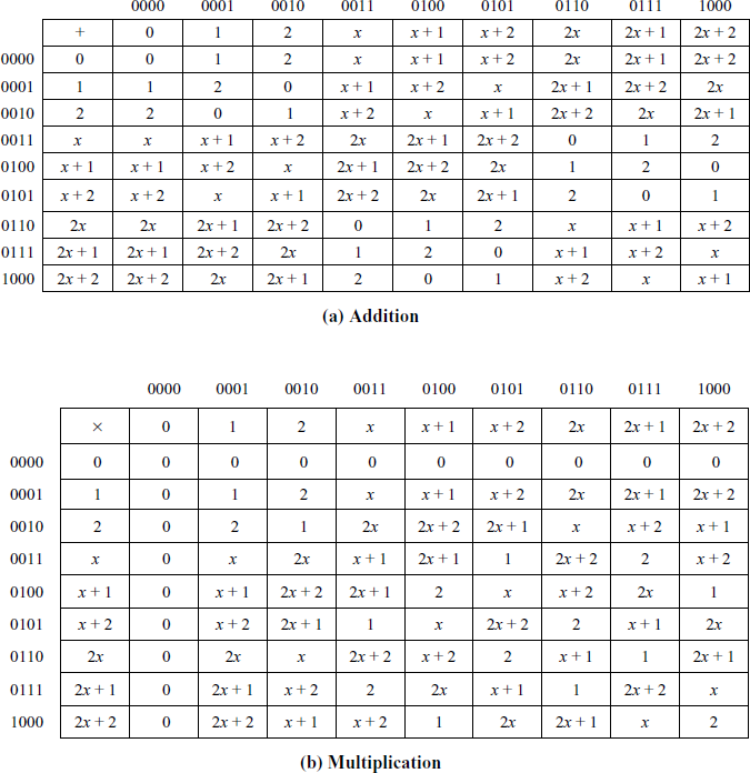
(b) Multiplication
Quadratic Residue: Suppose p is an odd prime and a is an integer, a is defined to be a quadratic residue modulo p, if  and the congruence
  has a solution
  . The value a is defined to be quadratic non-residue modulo p, if
  is not quadratic residue modulo p.
Example 2.32:
What are the quadratic and non-quadratic residues of Z11?
Solution

Therefore,
- Quadratic residues modulo 11 are,

- Quadratic non-residues modulo 11 are,

Theorem 2.6: Let p be an odd prime. Then, a is a quadratic residue modulo p, If

Legendre Symbol: Suppose p is an odd prime. For any integer a, define the Legendre symbol  by,
by,

Jacobi Symbol:
It is convenient to extend the Legendre symbol  to a symbol
  , where n is an arbitrary odd integer. This generalization is called the Jacobi symbol. Whenever n is an odd prime, we take
  to be the Legendre symbol. Let a be an integer, then the Jacobi Symbol
 is defined to be,

Example 2.33:
Consider the Jacobi symbol,  The prime power factorization of 9975 is,
  .
.


2.4.6 Continued Fraction
Continued fraction is used to express numbers and fractions. The continued fraction is an expression of the form,

ai and bi are either rational (or) real numbers. If all bi are ‘1’, then the continued fraction is called simple continued fraction. If the expression contains finite number of terms, then it is known as a finite continued fraction. Otherwise, it is called an infinite continued fraction. In a finite continued fraction, the iterative process of representing a number is terminated after finitely many steps by using an integer. In contrast, the iterative process is executed for an infinite number of steps in an infinite continued fraction. A simple continued fraction is of the form

For example, the continued fraction expression for the irrational number  is as follows:

Example 2.34:
Find the continued fraction of  .
.
 =
= = 3 +
= 3 + 
= 3 + 
= 3 + 
Example 2.35:
Find the continued fraction of  .
.
 = 4 +
= 4 + 
= 4 + 
=4 + 
=4 + 
2.5 Primality Testing Methods
Primality testing method is a method to find and to prove whether the given number is a prime number or not. There are two types of algorithms, namely deterministic and probabilistic algorithms to check the primality of a given number. This section discusses about both deterministic and probabilistic types of algorithms. Depending upon the size of prime numbers, there are various methods used to find prime number in an efficient way. Primality testing is an important method because prime numbers are used in many cryptographic algorithms such as rivest, shamir and adleman (RSA), Diffie–Hellman and pretty good privacy (PGP).
2.5.1 Naive Algorithm
Naive algorithm is used to divide the given input number p by all the integers starting from 2 to  If any one of them is a divisor, then the input number p is not a prime. Otherwise, it is considered as a prime number. The naive algorithm is also called trial division. Algorithm 2.5 explains about the naive algorithm.
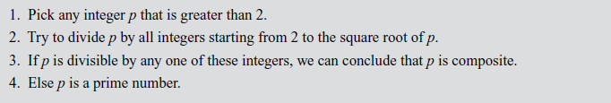
If p is not prime, then it factors as  , in particular one of the numbers a or b must be at most
  Hence, we actually only need to do
  divisions (2, 3, 4, ... ,
 ) in order to test whether or not a number is prime. The main limitation of this approach is that all numbers must be tested up to the square root of p, which is a time-consuming process. Therefore, this is fast enough when a small number of integers are given as input to test for primality. But as the number of test cases grow, this algorithm proves to be very slow.
Example 2.36:
Find the primality test for the number 100 using naive algorithm.
Solution
- 1. Select the integers 2, 3, ...
 (Square root of p).
 - Divide the input number 100 by all integers starting from 2 to 10.
Case 1:
 = 50 (100 is divisible by 2). Therefore, 100 is not a prime number.
Example 2.37:
Find the primality test for the number 47 using naive algorithm.
Solution
- 1. Select the integers 2, 3, …
 (Square root of p).
 - Divide the input number 47 by all integers starting from 2, 3, ..., 6.
Case 1:
 = 23.33 (47 is not divisible by 2)
Case 2:
 = 15.66 (47 is not divisible by 3)
Case 3:
 = 11.75 (47 is not divisible by 4)
Case 5:
 = 9.4 (47 is not divisible by 5)
Case 6:
 = 7.8 (47 is not divisible by 6)
Therefore, 47 is a prime number.
2.5.2 Sieve of Eratosthenes Method
For very small prime numbers, we can use the ‘Sieve of Eratosthenes’ method. This method is best method for small numbers, say all those less than 10,000,000,000. Algorithm 2.6 explains about the Sieve of Eratosthenes method.
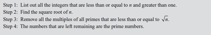
Example 2.38:
Find all the prime numbers less than or equal to 100 using the Sieve of Eratosthenes method.
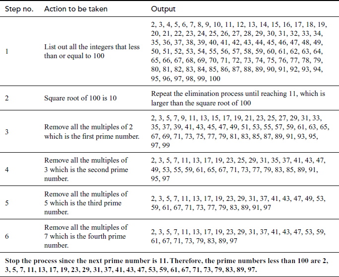
This method is so fast because there is no need to store a large list of primes on a computer. However, an efficient implementation is necessary to find them faster by avoiding the process of writing numbers in a storage area.
2.5.3 Fermat’s Primality Test
Fermat’s Theorem
If p is a prime and p does not divide a which is a natural number, then 
For example,  since 11 is a prime number and 11 does not divide 2.
Example 2.39:
Check that if the given number 12 is a prime number or not using Fermat’s theorem.
Solution
In order to find whether 12 is a prime number or not, we have to check  is equal to 1 or not, where a is
  . If it is equal to 1, then it is called a prime number. Otherwise, it is called a composite number. Consider a = 5, Then
  . Therefore, the given number is not a prime number.
Fermat’s theorem is a powerful test for compositeness. For example, Given n > 1 and a > 1 calculate an- 1 mod n. If the result is not one modulo n, then n is a composite number. If the result is one modulo n, then n might be prime and hence n is called a weak probable prime base a. In 1891, Lucas turned Fermat’s Little Theorem into a practical primality test. Lucas’ test is strengthened by Kraitchik and Lehmer.
Theorem 2.7: Let n 1 1. If for every prime factor q of n – 1 there is an integer a such that  and
and  is not 1 (mod n), then n is prime.
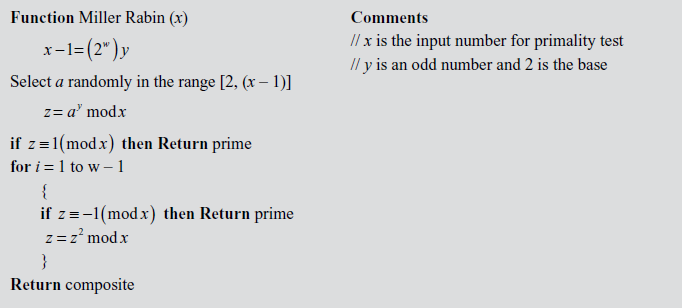
2.5.4 Miller–Rabin Primality Test
Rabin developed a new primality test called Miller–Rabin primality test. This test was based on Miller’s idea. The Miller–Rabin primality test is a probabilistic algorithm like Solovay–Strassen and it relies on equality or a set of equalities. This test holds true only for the prime numbers which is a fast method of determining the primality of a given number by using a probabilistic method. This method is advantageous over all the other primality testing methods discussed earlier. Algorithm 2.7 explains about the Miller–Rabin primality test.
Example 2.40:
Find the primality test for the number 1729 using Miller–Rabin method.
Solution
Let number to be tested for primality x = 1729
As per the algorithm, (x – 1) = (1729 − 1) = 1728 = 26 × 27
where  .
.
Let 
Let = 645
= 645
b = 645 ≠ 1
Therefore, as per Miller–Rabin algorithm, the operation  has to be done for 5 iterations since w = 6. If we do not get the answer of z = 1 or z = –1 in these five iterations, then the number can be concluded as a composite number.
Iteration 1: z = 6452 mod 1729 = 1065
Iteration 2: z = 10652 mod 1729 = 1
Since, we get the answer of z = 1 in second iteration itself, the number 1729 can be concluded as a prime number.
Example 2.41:
Find the primality test for the number 7 using Miller–Rabin method.
Solution
Let x = 7 (number to be tested for primality)
As per the algorithm, (x – 1) = (7 − 1) = 6 = 21 × 3
where 

Let a = 2 where 
z = 23 mod 7 = 1
Since the value of z = 1, as per Miller–Rabin algorithm 7 can be concluded as a prime number.
Example 2.42:
Find the primality test for the number 82 using Miller–Rabin method.
Solution
Let x = 82 (number to be tested for primality)
As per the algorithm, (82 − 1) = 81 = 33 × 3
where 

Let a = 2, z = 23 mod 82 = 8 ≠ 1
Since, the value of z ≠ 1, as per Miller–Rabin algorithm the operation  has to be done for 3 iterations. If we do not get the answer of z = 1 in all these three iterations, then the number can be concluded as a composite number.
Iteration 1: z = 82 mod 82 = 64
Iteration 2: z = 642 mod 82 = 78
Iteration 3: z = 782 mod 82 = 16
Since we do not get the value of z as 1 in all three iterations, the number 82 can be concluded as a composite number.
Example 2.43:
Find the primality test for the number 729 using Miller–Rabin method.
Solution
Let x = 729 (number to be tested for primality)
As per the algorithm, (729 − 1) = 728 = 23 ×91
where x = 729, w = 3, y = 91.
Let
z = 33 mod 729 = 27 ≠ 1
Therefore, the operation  has to be done for 3 iterations. If we do not get the answer of z = 1 in all these three iterations, then the number can be concluded as a composite number.
Iteration 1: z = 272 mod 729 = 0 ≠ 1
Since we get the value of z as 0 in the first iteration, the preceding two iterations will also get the value of z as 0 only. Therefore 729 can be concluded as a composite number from the first iteration itself.
2.6 Factorization
Factorization of a given positive integer n is the process of finding out positive integers x and y such that the product of x and y equals to n and also x and y are greater than 1. The values x and y are called factors (divisors) of n. Factorization can be performed for any positive integer greater than 1. If a number is not factored, then it is called a prime number. For example, a number  can be factored into two positive integers x and y, where
  and
and  However, the number
  cannot be factored since it is a prime number. Factorization of a composite number does not necessarily produce unique results. For example, the number
  can be factored as the product of the two composite numbers
  and
and . In the same way, the same number
  can be factored as the product of the prime number
  and the composite number
 (because,
  ). Similarly, the same number
  can also be factored as
 . But the prime factorization of a given number gives the same result. However, in prime factorization method, the output of factorization algorithm is to be checked to find whether it is a composite or prime number.
2.6.1 Prime Factorization Method
Prime factorization can be obtained for the above results by further factoring the factors that happen to be a composite number. For example, prime factorization of the number  contains three answers as shown in Figure 2.5 that are same. Therefore, from the first result
 , the composite numbers 15 and 4 can be further factored into prime factors like
 . In the same way, from the second result (
 ), the composite number 20 can be factored as
 . So,
. So,  , which is same as that of the previous result. Similarly, the third result
  can also factored as
  . Figure 2.5 shows the diagrammatic representation of the working example for the number 60. Factoring a composite integer is a challenging problem and also it takes more computing power. In addition to this, composite numbers are not used in most of the cryptographic algorithms. There are many factorization algorithms to find factors or divisors of a given positive integer. Among the many factorization algorithms, this bookwork focuses on about prime factorization, trial division, Fermat’s factorization and Pollard’s rho method. Prime factorization is a method used to find the GCD and LCM (least common multiple) of the given two positive integers. Prime factorization is explained in Section 2.1.4. Remaining factoring methods are explained in this section.
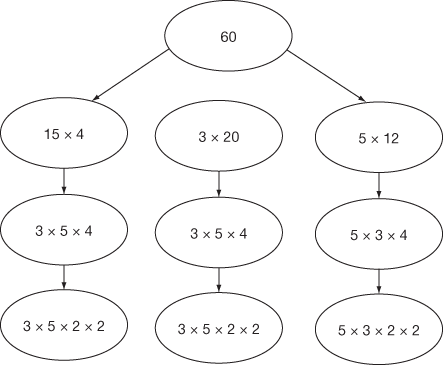
Figure 2.5 Prime factorization of the number 60
2.6.2 Trial Division Method
It is the simplest way of finding the factors or divisors of a given positive integer n. This method is a very similar method to Sieve of Eratosthenes method. This method divides the given number of all the integers that are greater than 1 and less than or equal to  .
.
Algorithm 2.8 explains about the trial division method. In this algorithm, two while loops are used and hence it takes more computation complexity.
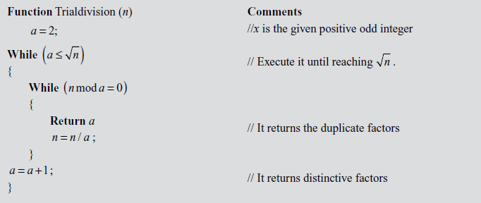
Example 2.44:
Factor the number 105 by using trial division method.
Trial 1:  ,
,  ,
,  . So, increment a value by 1.
Trial 2:  ,
,  ,
,  . So, return the value 3 as a factor.

 . So, increment a value by 1.
Trial 3:  ,
,  ,
,  . So, increment a value by 1.
Trial 4:  ,
,  ,
,  . So, return the value 5 as a factor.

 . So, increment a value by 1.
Trial 5:  ,
,  ,
,  . So, increment
  value by 1.
Trial 6:  ,
,  ,
,  . So, return the value 7 as a factor.

 . So, increment
  value by 1.
Trial 7:  ,
,  ,
,  . So, increment
  value by 1.
Trial 8:  ,
,  ,
,  . So, increment
  value by 1.
Trial 9:  ,
,  ,
,  . So, increment
  value by 1.
Trial 10:  ,
,  ,
,  . Stop this process because,
  .
.
Therefore, the factors are 3, 5 and 7.
2.6.3 Fermat’s Factorization Method
Fermat’s factorization method was developed by Pierre de Fermat. Fermat’s factorization method uses a piece of information that any number can be expressed as the difference between two squares. For example, the given positive integer  can be expressed as
  and
and and also any one of the factors must not be 1. So, the number n can be written as
  This method is used to find the factors of a given positive odd integer only.
This method is a simple to implement, but it would be slower than trial division (worst case). Algorithm 2.9 explains about the Fermat’s factorization method. In this algorithm,  (Because,
  ) value is computed in each trial until b value becomes a perfect square value. Finally, this algorithm returns any one of the factor values after subtracting or adding
  value from the value of a.
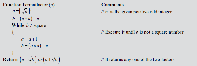
Example 2.45:
Factor the number 105 by using Fermat’s factorization method.
 .
.  =
=  =
= 
 .
.
Since b is a square, it would return  So,
So,  and
and  = 11 + 4 = 15. Therefore, the numbers 7 and 15 are the factors of the given number
 .
.
Example 2.46:
Factor the number  by using Fermat’s factorization method.
n = 1575.  =
=  =
= 

Since b is a square it would return  So,
So,  and
and  = 40 + 5 = 45. Therefore, the numbers
  and
and  are the factors of the given number
 .
.
Example 2.47:
Factor the number  by using Fermat’s factorization method.
First loop:  .
.  =
=  =
= 

Since  is not a square number, next trial is to be executed.
Second loop:  .
.

Since b is a square number, it would return and
and  . Therefore, the numbers
  and
and  are the factors of the given number
 .
.
2.6.4 Pollard’s rho Method
This factorization method was developed by John Pollard in the year 1974. It was developed based on the two assumptions:
1. Assume that there are two integers  and
and  such that
  divides
  but it does not divide by the given number
  .
.
2. It is clear to understand that  . Since,
  divides
  it can be written as
  . Moreover,
  or a factor of
  since
since  is not divided by the given number
  .
.
Algorithm 2.10 explains about the Pollard’s rho factorization method. In this algorithm, two functions are used, namely Factor and Pollard_rho. Among the two functions, the first function factor is used to find the factors of a given positive integer. The second function is used to implement Pollard rho factorization method. Initially, the given input number is passed onto the main function ‘Factor’ which calls the subfunction Pollard_rho. In the subfunction Pollard_rho, the variables  are initialized to compute the divisors. Two equations are declared and implemented in this subfuction. One equation is
  and another equation is c
 which is executed twice in the subfunction. By using the computed values of b and c, the GCD value is computed to find any one of the divisors of a given number. The process is executed until the divisor equals to 1. This function returns the divisor value to the main function when any of the divisor is found where the first function factor is executed in a recursive procedure.
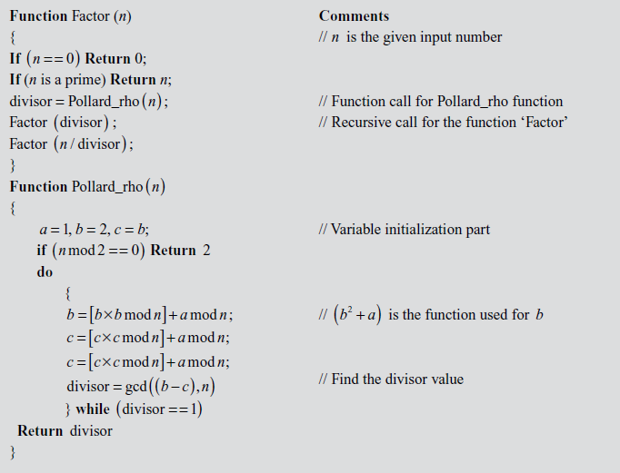
Example 2.48:
Find the factors of (60) using the Pollard’s rho method.
Solution

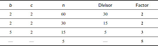
Example 2.49:
Find the factors of  using the Pollard’s rho method.
Solution

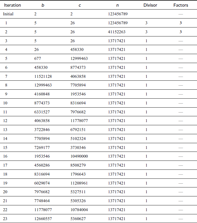
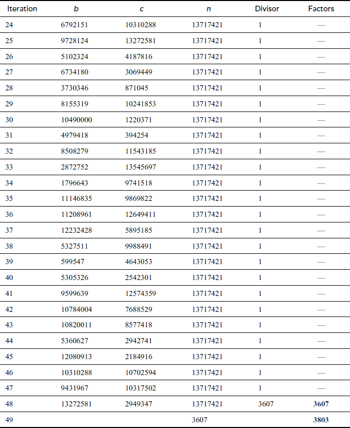
Key Terms
Additive group
Algebraic structures
Backward secrecy
Chinese remainder theorem (CRT)
Commutative ring
Computation complexity
Congruence
Continued fraction
Euclid’s algorithm
Euler’s theorem
Exponentiation
Extended Euclidean algorithm
Factorization
Fast modular exponentiation
Fermat theorem
Fermat’s factorization
Fermat’s primality test
Fields
Finite continued fraction
Forward secrecy
Galois fields (GFs)
Greatest common divisor (GCD)
Group
Infinite continued fraction
Jacobi symbol
Legendre symbol
Miller–Rabin primality test
Modular exponentiation
Multicast
Multiplicative group
Naive algorithm
Pollard rho
Polynomial
Primality testing
Prime factorizations
Quadratic residue
Ring
Sieve of Eratosthenes
Trial division method
Summary
- In this chapter, we explained about the foundation of basic number theory and its branches. This concept is necessarily discussed in this chapter before explaining about cryptographic algorithms.
- One of the important concepts in number theory is congruences.
 is congruent
  to
to  if and only if
  is a multiple of n.
 - Exponentiation is a type of operation where two elements are used in which one element is considered as base element and another element is considered as exponent element.
- The GCD of two or more integers is defined as the greatest positive integer that divides the numbers without a remainder. Among the various methods of GCD computation, the Euclid’s algorithm is an efficient method.
- The extended Euclidean algorithm is an efficient method of finding the modular inverse of an integer. The Euclid’s algorithm can be extended to give not only
 , but also two integers x2 and y2 such that
  .
. - The Chinese remainder theorem (CRT) is used to find a common value from a system of congruences. CRT is mainly used in coding theory and cryptography.
- Fermat’s theorem is mainly used to solve modular exoneration problems when the base is considered as a, moduli are considered as prime p and p should not divide a.
- Euler’s phi function
 returns the number of integers from 1 to n, that are relatively prime to n.
 - Cryptographic algorithms are mainly working on the basis of algebraic structures. An arbitrary set with one or more limited operation defined on it with certain axioms is called an algebraic structure.
- Three types of algebraic structures, namely groups, rings and fields are discussed in this chapter.
- A group is a set
 together with a binary operation *25on
  that satisfies four axioms, namely closure, associative, identity and the inverse element.
 - The groups can also be divided into two types, namely finite groups and infinite groups. There are two types of groups used in cryptographic algorithms, namely additive group and multiplicative group.
- A ring R is a set of elements together with two binary operations addition (+) and multiplication ( × ) operations that satisfies six axioms, namely closure, associative, commutative, multiplication operation distribute over the addition, identity and the inverse element. The ring is divided into two types, namely commutative ring and division ring.
- A field F is a set of elements together with two binary operations addition (+) and multiplication (×) operation that satisfies six axioms, namely closure, associative, commutative, multiplication operation distribute over the addition, identity and the inverse element.
- Field is of the form GF(pn), where the ‘GF’ represents a ‘Galois Field’. The addition and subtraction operations in GF(pn) are performed by adding or subtracting two polynomials together, and reducing the result modulo the attribute p.
- Multiplication operation in a Galois field GF(2n) is performed by multiplication followed by a modulo division with respect to an irreducible polynomial used to define the Galois field GF(2n).
- Continued fraction is used to express numbers and fractions. If the expression contains a finite number of terms, then it is known as a finite continued fraction. Otherwise, it is called an infinite continued fraction.
- Primality testing method is a method to find and to prove whether the given number is a prime number or not.
- There are four types of primality testing methods, namely naive algorithm, Sieve of Eratosthenes method, Fermat’s primality test and Miller–Rabin primality test. Among the four methods, Miller–Rabin primality test is an efficient method.
- Factorization of a given positive integer n is the process of finding out positive integers x and y such that the product of x and y equals to n and also x and y are greater than 1.
- The trial division method is the simplest way of finding the factors or divisors of a given positive integer n.
- Fermat’s factorization method uses a piece of information that any number can be expressed as the difference between two squares such as
 .
. - Pollard rho is an efficient factorization method which was developed by John Pollard in the year 1974.
Review Questions
- Calculate 216 mod 123.
- Calculate 314 mod 30.
- Use the modular exponentiation algorithm to calculate 1519 mod 37.
- Find gcd(143, 227), gcd(8, 182), gcd(125, 87) using Euclidean method.
- Find the values of x2 and y2 from the given values (a, b) = (8, 182) by using extended Euclidean algorithm.
- Find the value of x2 and y2 from the given values (a, b) = (16, 10374) by using extended Euclidean algorithm.
- Find the x value for the equation x2 ≡ 1 (mod 35) using CRT.
- Find the x value for the system of congruences.
-


- Solve the system of simultaneous congruences.
-

-

-

-

- Compute Euler’s totient function for the value 1729.
- Find
 .
. - Solve the value of
 .
. - Solve the value of

- How additions and multiplications are performed in GF(2n)? Explain in detail.
- Solve
 using Jacobi–Legendre symbol.
 - Factor the numbers 12345 and 67890.