Table of Contents for

NoSQL and SQL Data Modeling: Bringing Together Data, Semantics, and Software

Chapter 17 NoSQL and SQL Physical Design

As you can see, the bulk of this book is spent explaining concepts of analysis and design, and teaching you how to represent things in the real world, and data about those things, in COMN models. Now we get to the final step that follows from analysis and design: expressing a physical database design in a COMN model. There are several goals for such a model:

1. We want the model to be as complete and precise as an actual database implementation, so that there’s no question how to implement a database that follows from the model. This is especially important if we want to support model-driven development.
2. We want assurance that the physical design exactly represents the logical design, without loss of information and without errors creeping in.
3. We want the database implementation to perform well, as measured by all the criteria that are relevant to the application. We want queries by critical data to be fast. We want updates to complete in the time allowed and with the right level of assurance that the data will not be lost. The physical design process is the place where performance considerations enter in, after all the requirements have been captured and the logical data design complete.

What’s Different about NoSQL?

The most obvious difference between NoSQL and SQL databases is the support, or lack of it, for the Structured Query Language (SQL). However, times have changed, and it’s no longer so easy to divide DBMSs into two strictly separate camps of SQL and NoSQL. Some NoSQL DBMSs have added SQL interfaces, to make it easier to integrate them into traditional database environments. The former distinction of ACID and BASE is melting away, as NoSQL DBMSs add ACID capabilities, and SQL databases provide tunable consistency to enable greater scaling. Finally, both SQL and NoSQL DBMSs are adding more ways to organize data. Some NoSQL DBMSs support tabular data organizations, and some SQL DBMSs support columnar and document data organizations.

As a result, the rejection of SQL has been softened, so that now “NoSQL” has been reinterpreted to mean “not only SQL”. This reflects the realization that it’s generally better to have a selection of physical data organization techniques at one’s disposal. Being able to arrange one’s data only as, say, a graph, can be just as limiting as being able to arrange one’s data only as a set of tables. It’s just as mistaken to have only a screwdriver in one’s toolbox as it is to have only a hammer. One wants a toolbox with a hammer, a screwdriver, a hex wrench, and many other tools as well.

So, rather than present all of these DBMS characteristics divided into two overly simplistic categories of NoSQL and SQL, I will present the full list of DBMS capabilities regardless of whether SQL is the main data language.

Database Performance

Our task as physical database designers is to choose the physical data organization that best matches our application’s needs, and then to leverage the chosen DBMS’s features for the best performance and data quality assurance. This might lead us to choose a DBMS based on the data organization we need. However, sometimes the DBMS is chosen based on other factors such as scalability and availability, and then we need to develop a physical data design that adapts our logical data design to the data organizations available in the target DBMS.

The task of selecting the best DBMS for an application based on all the factors below and the bewildering combinations of features available in the marketplace, at different price points and levels of support, is far beyond the scope of this book to address. This chapter will equip you to understand the significance of the features of most of the DBMSs available today, and then—more importantly for the topic of this book—show you how to build physical models in COMN that express concrete representations of your logical data designs.

Physical design is all about performance, and there are several critical factors to keep in mind when striving for top performance:

• scalability: Make the right tradeoffs between ACID and BASE, consulting the CAP theorem as a guide. Know how large things could get—that is, how much data and how many users. You will need to know how much of each type of data you will accumulate, so that you can choose the right data organization for each type.
• indexing: Indexing overcomes what amounts to the limitations of the laws of physics on data. If a field is not indexed, you will have to scan for it sequentially, which can take a very long time. Add indexes to most fields which you want to be able to search rapidly, and consider the various kinds of indexes the DBMS offers you. But be aware of the tradeoffs that come with indexes.
• correctness: Make sure the logical design is robust before you embark on the physical design. There’s nothing worse than an implementation that is fast but does the wrong thing. In this context, “robust” means complete enough that we don’t expect that evolving requirements will require much more than extension of the logical design.

ACID versus BASE and Scalability

ACID

Almost all SQL DBMSs, plus a few NoSQL DBMSs, implement the four characteristics that are indicated by the acronym ACID: atomicity, consistency, isolation, durability. These four characteristics taken together enable SQL databases to be used in applications where the correctness of each database transaction is absolutely essential, such as financial transactions (think purchases, payments, and bank account deposits and withdrawals). In those kind of applications, getting just one transaction wrong is not acceptable.

Here is a guide to the four components of ACID.

Atomicity

A DBMS transaction that is atomic will act as though it is indivisible. An update operation that might update a dozen tables will either succeed completely or fail completely. Either all affected tables will be updated, or, if for some reason the update cannot completely succeed, tables that were updated will be rolled back to their pre-update state. A transaction might not complete because of errors in the update, or because a system crashed. It does not matter: An atomic transaction will appear to a DBMS user as if it either completely succeeded or completely failed.

Consistency

A DBMS can enforce many constraints on data given to it to store. The most fundamental constraints are built-in type constraints: string fields can only contain strings, date fields can only contain dates, numeric fields can only contain numbers, etc. Additional constraints can be specified by a database designer. We’ve talked a lot about foreign-key constraints, where a column of one table may only contain values found in a key column of another table. There can be what are called check constraints, which are predicates that must be true before data to be stored in a table is accepted.

Consistency is the characteristic that a DBMS exhibits where it will not allow a transaction to succeed unless all of the applicable constraints are satisfied. If, at any point in a transaction, a constraint is found which is not met by data in the transaction, the transaction will fail, and atomicity will ensure that all partial updates that may have already been written by the transaction are rolled back.

Isolation

Isolation is the guarantee given by a DBMS that one transaction will not see the partial results of another transaction. It’s strongly related to atomicity. Isolation ensures that the final state of the data in a database only reflects the results of successful transactions; isolation ensures that, if a DBMS is processing multiple transactions simultaneously, each transaction will only see the results of previous successfully completed transactions. The transactions won’t interfere with each other.

Durability

Durability is the guarantee that, once a transaction has successfully completed, its results will be permanently visible in the database, even across system restarts and crashes.

BASE and CAP

ACID sounds great, and it really is great if one has an application where preserving the result of every transaction is critical. But ACID comes at a cost. It is difficult to build DBMSs that can leverage large farms of parallel servers to increase processing capacity, while achieving ACID. Large farms of parallel servers are needed to support millions of users and billions of transactions. Such databases are seen in companies like Facebook and Amazon. These large databases are designed to scale horizontally, meaning that greater performance is achieved by putting many computers side-by-side to process transactions in parallel, and the data is replicated many times over so that multiple copies may be accessed simultaneously for retrieving requested data. This is in contrast to the traditional approach of scaling vertically, meaning that a faster computer and larger storage are used for the DBMS. There are limits on how fast and large a single system can be made, but the limits are much higher on how many computers and how much storage can be set side-by-side.

Horizontal scaling is great, but the CAP theorem, put forward by Eric Brewer in 2000 [Brewer 2012], proves that, in a distributed DBMS, one may only have two of the following three attributes:

• consistency: This is a specialized form of the consistency of ACID. It does not refer to the enforcement of consistency constraints. Rather, it is the requirement that, in a DBMS that has many copies of the same data, all of the copies match each other. In a horizontally scaled database, one can guarantee that all the copies match each other, but only if either availability or partition tolerance is sacrificed.
• availability: With lots of computers accessing lots of storage over many network connections, there are bound to be failures at various points. That much hardware just has to have some pinpoint failures from time to time. But the motivation for having so many computers and so many copies of the same data is that, for any data request, there’s a good likelihood that some working computer can access some copy of the data and satisfy the request, even if some of the computers are down or some of the storage is unavailable. 100% availability can be achieved, even in a network with some failures, but only if either consistency or partition tolerance is sacrificed.
• partition tolerance: A partitioning of a distributed system is a case where a network failure causes one subset of the computers in the distributed system to be unable to communicate to the rest of the computers. The result of a partitioning is that copies of the database maintained by different computers can get out of sync with each other. An update completed in one set of computers will be missed by the other set. A DBMS can be programmed to tolerate partitioning, but only at the sacrifice of either consistency or availability.

The CAP theorem forces you to see that you can’t have your cake and eat it too. If your plan is to scale a DBMS horizontally by linking lots of computers side by side to maintain lots of copies of the same data, then you have to choose just two features out of consistency, availability, and partition tolerance.

Most NoSQL databases are designed to scale horizontally, and so because of CAP they can’t offer ACID. They are described as achieving BASE (cute acronym):

• Basic Availability: Most of the data is available most of the time.
• Soft state: Unlike ACID, a “commit” of an update to a database might not always succeed. Some updates will be lost.
• Eventual consistency: After some internal failure, out-of-sync copies of data will eventually “catch up” with the correct copies.

BASE sounds a little scary, but sometimes it’s all that’s needed. For example, Facebook serves hundreds of millions of users, and probably couldn’t do so effectively with ACID-strength guarantees. So they allow users to post with only a soft-state guarantee. Every now and then, a user’s post gets lost. (It has happened to me.) The downside is minimal: a few users are occasionally slightly annoyed by having to re-type a short update. As long as this doesn’t happen too often, Facebook is able to fulfill its mission of enabling hundreds of millions of users to share their personal lives and thoughts. This would not be possible with a traditional ACID approach.

A particular application might use both an ACID DBMS and a BASE DBMS, in combination, to achieve a certain mission. For example, a retail Web site might deliver product information and user reviews using a BASE DBMS, but run purchases and financial transactions on an ACID DBMS. A user would probably tolerate a review being lost, but not a purchase being lost or an account double-charged for one purchase.

NoSQL and SQL Data Organization

Under the covers, NoSQL and SQL DBMSs all use the same set of data structures that were worked out decades ago for organizing data for fast access. These structures include things called trees, linked lists, queues, arrays, hashes—and those venerable data structures, tables. What distinguishes DBMS types from each other is how they present these varied data storage structures to the DBMS user. NoSQL databases can be categorized into four types of data organization:

• key/value: an extremely simple data organization, where each record has a single key data attribute which is indexed for high-speed searching, and a “value”, which is really just an object for storing arbitrary data whose structure is not known to the DBMS
• graph: storage of data defining graph nodes and edges
• document: storage of data in a form similar to ordinary text documents; usually using lots of nesting
• columnar: storage of data as columns of a table rather than in the traditional organization of rows of a table

When we add tables to this list—the traditional data organization of SQL databases—we see that we have five ways to organize our data physically.

Key/Value DBMS

A system that organizes data as key/value pairs is arguably the simplest means of managing data that can justify calling the system a database management system. The main focus of a key/value DBMS is on providing sophisticated operations on key values, such as searching for exact key values and ranges of key values, searching based on hashes of the key values, searching based on scores associated with keys, etc. Once the application has a single key value, it can speedily retrieve or update the “value” portion of the key/value pair.

Key/value terminology is somewhat problematic, since the keys themselves have values. In reality, the “value” portion of key/value is just an object of some class that is unknown to the DBMS.

Because of the simplicity of key/value DBMSs, it is relatively easy to achieve high performance. The tradeoff is that the work of managing the “value” is left to the application. Some DBMSs are beginning to provide facilities for managing the “value” portion as JSON text or other data structures.

Mapping a logical record type to a model like this involves the following considerations:

• Each physical record class can have only one key, which could consist of one component or of a set of components treated as a unit (in other words, a composite key). This will be the only component that can be searched rapidly. If records need to be found by the value of more than one component, the data might have to be split into several physical record classes.
• To the DBMS, the “value” component is a blob, but to the application it’s quite important. Therefore, it will behoove the designer and implementer to fully define the “value” components of the logical record.

Because key/value DBMSs don’t support foreign key constraints, a greater burden is put on the application to ensure that only correct data is stored in a key/value database.

Graph DBMS

A graph DBMS supports the organization of data into a graph. There are only two kinds of model entities in a graph: nodes and edges. Graph data is usually drawn using ellipses or rectangles to represent nodes and lines or arcs to represent edges. In contrast to common practice in most applications of data modeling, graph data models usually depict entity instances rather than entity types. Figure 17-1 shows some graph data expressed using the COMN symbols for real-world objects (Sam), simple real-world concepts (Employee Role), and data values (2016-01-01).

Figure 17-1. A Data Graph

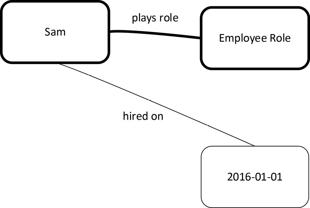
Data expressed in the Resource Definition Framework (RDF), described in chapter 8, is especially suited to representation as a graph. An RDF triple maps directly to a graph. The subject and object of a triple are graph nodes, and the predicate is an edge. In RDF terms, the graph of Figure 17-1 illustrates two triples.

A data graph is valuable for expressing and exploring the relationships between various entities, and between entities and data attributes about them. Representing data in a graph makes it possible to use dozens of graph algorithms to analyze the data. Graph algorithms can be used to find the shortest way to visit many points, to search for similarities in large quantities of data, or to find graph nodes that are strongly related to each other. A data graph makes no distinctions between entities and their attributes, or, for that matter, data attributes. If the data in question is to be represented in a graph database, then such distinctions do not matter. However, one must be aware that such distinctions are lost in a graph database. Whether or not that matters depends on the nature of the application.

If one wishes to illustrate the permissible values of nodes in a graph database—in other words, add type and class information—one can do this by using the COMN symbols for types and classes. Figure 17-2 below expresses the expected types of the actual graph data in Figure 17-1.

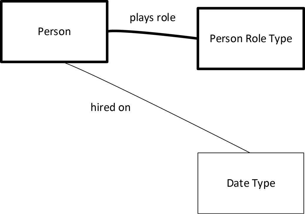
Figure 17-2. A Model of a Graph Type

Figure 17-2 is a mini-ontology, in that it expresses relationships which exist between a class of real-world objects (Person), a type of behavior of persons in the real world (Person Role Type), and a type of data (Date Type). As mentioned in chapter 8, COMN can be used as a graphical notation for ontologies.

Document DBMS

At its interface, a document DBMS stores and retrieves textual documents. A document DBMS usually supports some partial structuring of documents using a markup language such as XML. Some so-called document DBMSs support JSON texts, often mistakenly called documents. A document is a primarily textual composite record type with possibly deep nesting. Usually, many of a document’s components are optional. It is straightforward to model any document’s structure in COMN as nested composite types; however, a non-trivial document might involve many types and might need to be split across a number of diagrams.

As with any database, speedy access to data will depend on important components being indexed. A database index is built and maintained by a DBMS by taking a copy of the values (or states) of all instances of a specified component or components, and recording in which documents those values are found. This is represented in COMN as a projection of data from the record or document collection to the index, and then a pointer back to the collection. DBMSs usually offer indexes in many styles. The particular index style can be indicated in the title bar of the index collection, in guillemets, as in «range index». This notation gives the class (or type) from which the current symbol inherits or is instantiated. See Figure 17-3 for an example. The Employee ID Index is defined as a physical record collection that is a projection from the full Employee Resume Collection of just the Employee ID component. The index is also an instance of a unique index, a class supported by the DBMS. The pointer back to the collection is implicitly indicating a one-to-one relationship from each index record to a document in the collection, which is true of a unique index. A non-unique index would require a “+” at the collection end of the arrow, indicating that one index record could indicate multiple documents or records in the collection.

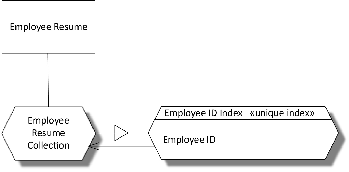
Figure 17-3. A Document Database Design with a Unique Index

Columnar DBMS

A columnar DBMS presents data at its query interface in the form of tables, just as a SQL DBMS does. The difference is in how the data is stored.

Traditional table storage assumes that most of the fields in each row will have data in them. Rows of data are stored sequentially in storage, and indexes are provided for fast access to individual rows.

Sometimes it would be better if the data were sliced vertically, so to speak, and each column of data were stored in its own storage area. A traditional query for a “row” would be satisfied by rapidly querying the separate column stores for data relevant to the row, and assembling the row from those column queries that returned a result. However, columnar databases optimize for queries that retrieve just a few columns from most of the rows in a table. Such queries are common in analytical settings where, for example, all of the values in a column are to be summed, averaged, or counted. Columnar databases optimize read access at the cost of write access (it can take longer to write a “row” than in a row-oriented database), but this is often exactly what is needed for analytical applications.

Consider, for example, a database of historical stock prices. These prices, once written, do not change, but will be read many times for analysis. In a row-oriented database, each row would repeat a stock’s symbol and exchange, as well as the date and open, high, low, and close prices on each trading day. A columnar database can store the date, open, high, low, and close each in their own columns and make time-series analysis of the data much more rapid.

Representing a columnar design in COMN involves modeling the columns, which are physical entities. This is quite straightforward to do, as a column is a projection of a table. Figure 17-4 below shows our example design, where the physical table class that represents the logical record type is shown projected onto a row class and five columnar classes.

Tabular DBMS

Let’s not forget about traditional tables as a data organization. Traditional tables can, of course, be used in SQL DBMSs, but increasingly NoSQL DBMSs support them, too.

The physical design of tabular data emphasizes several aspects for performance and data quality:

• indexing: Probably the most important thing to pay attention to in a tabular database design is to ensure that all critical fields are indexed for fast access. Add indexes carefully, because each index speeds access by the indexed data, but also increases the database size and slows updates.
• foreign keys: Foreign key constraints are valuable mechanisms for ensuring high data quality. They were covered in chapter 15.
• partitioning: Many DBMSs enable the specification of table partitions (and even index partitions). The idea is that each partition, being smaller than the whole table, can be searched and updated more quickly. Any query is first analyzed to determine which table partition(s) it applies to, and then the query is run just against the relevant partition.

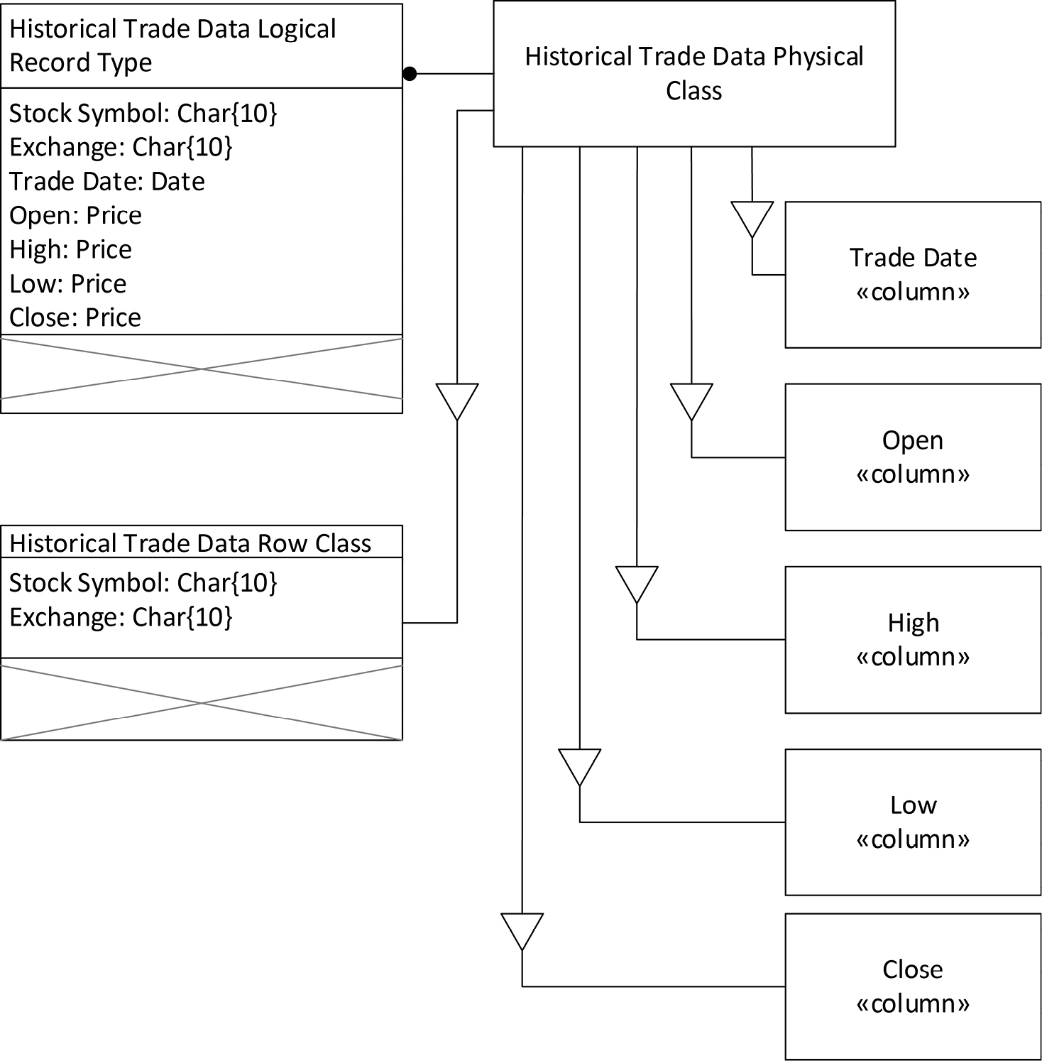
Figure 17-4. A Columnar Data Design

As explained under document DBMSs, an index is a projection of the table data into another table. The index type is given in the shape’s title section, surrounded by guillemets.

Foreign key constraints were covered in depth in chapter 15. A physical design illustrating foreign key constraints would use the same symbols but solid outlines to connote physical classes implemented by the DBMS, rather than the dashed outlines used in logical data design. The only new thing to consider is how to model partitioning a table by rows—so-called horizontal partitioning. Each partition can be thought of as a table in its own right, containing a subset of the data. The subset is usually defined by some restriction on the data based on a value found in the data, such as a date. Figure 17-5 illustrates a horizontally partitioned row-oriented table.

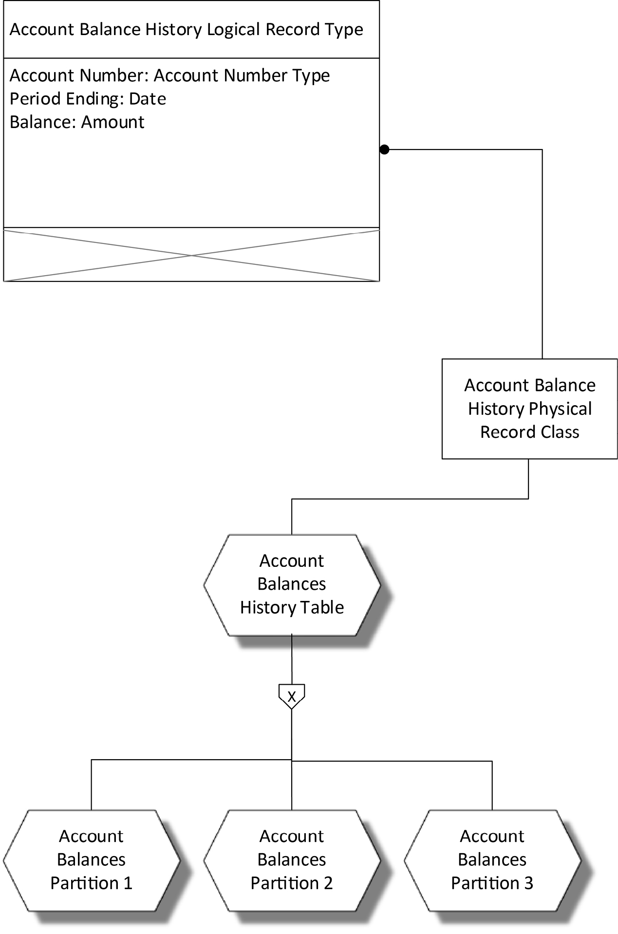
Figure 17-5. A Partitioned Row-Oriented Table

Summary

COMN’s ability to express all the details of physical design for a variety of data organizations means that the physical implementation of any logical data design can be fully expressed in the notation. COMN enables a direct connection to be modeled between a logical design and a physical design in the same model, enabling verification that the implementation is complete and correct. The completeness of COMN means that data modeling tools could use the notation as a basis for generating instructions to various DBMSs to create and update physical implementations. This makes model-driven development possible for every variety of DBMS.

References

[Brewer 2012] Brewer, Eric. “CAP Twelve Years Later: How the Rules Have Changed.” New York: Institute of Electrical and Electronic Engineers: IEEE Computer, February 2012, pp. 23-29.

Key Points Physical database design is the place where performance becomes paramount. Physical design should not begin until a robust logical data design has been completed. There are many physical data organizations available for implementation, including key/value, document, graph, columnar, and row-oriented tabular. Some DBMSs are specialized for exactly one form of data organization, and some are hybrid, supporting multiple organizations. DBMSs vary to the extent to which they can be scaled in size, and to the extent they support ACID and BASE transactional characteristics. DBMS selection must sort through the various intersections of data organization, ACID/BASE, scaling, performance, price, and support that appear in the marketplace. Matching a DBMS’s data organization style to an application’s needs is just one important aspect of DBMS selection. Many DBMSs achieve speed and scale by omitting features that applications have often used to achieve high data quality, such as type safety and foreign key constraints. Be sure to consider these aspects when selecting a DBMS. Data to be stored in a key/value DBMS should be modeled in its entirety, even though the DBMS sees the “value” only as a blob, because the application will need to know the structure of the “value”. Graph data can be modeled in COMN using value and object symbols. A graph schema can be modeled with a graph of COMN type and class symbols. Database indexes, whether for documents or tables, are modeled in COMN as projections of the main record collection. A DBMS-specific index class can be noted in a shape’s title, surrounded by guillemets (« »). A columnar data organization is modeled as projections of the record class onto multiple column classes. A horizontally partitioned row-oriented table is shown as a set of exclusive subsets of the main table.