Table of Contents for

NoSQL and SQL Data Modeling: Bringing Together Data, Semantics, and Software

Chapter 16 The Relational Theory of Data

We’ve gotten quite far in our investigation of data models, including discussions of what data and information are, and what relationships are. It’s finally time to take a look at the fundamental theory behind all of this.

We’ve already established, and the world has already proven, that you can do a lot with data without understanding relational theory. It’s also true that you can do a lot with water power without understanding the water molecule, H2O. So why are we bothering at this juncture to look at relational theory? Because so much thinking will be clarified, and so many new vistas will open before us, when we understand what relational theory is all about.

For the NoSQL aficionados among my readers, you should realize that relational theory matters as much to NoSQL databases as it does to SQL databases—even more so, in one sense. Relational theory is a theory of data that matters whether you’re storing your data in a document, a graph, or a table. SQL is strongly associated with relational theory, but that doesn’t mean that the theory only works with SQL. It works whenever there’s data. You don’t know it yet, but if you’ve read the book this far, you’ve already encountered many of the important concepts in relational theory.

In my experience, I’ve often seen folks struggle to understand relational theory. If you’ve read this far in this book and understood most of it, you’ve already grasped concepts that are more difficult than those in relational theory. The reason that relational theory escapes many people is because of one of the greatest terminological tragedies in our field, which is that, in relational theory, a “relation” is not the same as a “relationship”! Once you get past that, the rest is relatively easy.

What is a Relation?

In overly simplistic terms, a relation is a table. So why do we use this fancy word “relation”, instead of the more easily understood term “table”? Because there are some important differences, namely:

1. The order of rows in a relation has no significance whatsoever, while the order of rows in a table may carry information.
2. The repetition of rows in a relation has no significance whatsoever, while the repetition of rows in a table may carry information.

Below I will explain these differences, and why they matter.

The Order of Rows

As soon as a list of data is written down on a piece of paper, it has an order; that is, the order in which the data is written down. But does that order mean anything? To understand this issue, we will consider two examples from everyday life.

Imagine a cash register receipt from a grocery store. See Figure 16-1 for an example of part of a cash register receipt.

TOMATO CAN 16 OZ	1.69
MILK 128 OZ	3.39
CARROTS 2.30 LB @ 0.69	1.59
TOMATO CAN 16 OZ	1.69
FACIAL TISSUE	4.59

Figure 16-1. Part of a Grocery Store Cash Register Receipt

When cash registers were mechanical devices that printed item prices on paper, cash register receipts showed the prices of grocery items in the order in which the cashier rang them up. This custom has been preserved even in the age of computerized registers and bar code scanners. Thus, not only does the printing on the paper register tape show each item purchased together with its price, but it also shows the order in which the items passed by the scanner. If, for some reason, we wished to re-order the items in the list, say by sorting them so that the least expensive item appeared first, we would lose track of the order in which they were rung up or scanned. We observe that there is information carried in the order of the items in the list. In contrast, consider a printed telephone directory. See Figure 16-2 for an example of part of a telephone directory.

Doe Jack 123 Main St.	555-1234
Doe Jane 222 Axle Ave.	555-9999
Doe John 27 Red House Ln	555-8877
Doe Joseph 1 Pennsylvania Rd	555-3333

Figure 16-2. Part of a Telephone Directory

This list also has an order. It is apparent that the order of this list is determined by sorting the names of telephone subscribers in alphabetical order. The telephone directory publisher established this order so that it is easy to find listings by name: one simply searches alphabetically through the directory for the name of the desired listing.

If you took a telephone directory, cut off the binding while leaving the contents of the pages intact, and shuffled the pages like a deck of cards, you would not lose any information. Every listing would still be in those pages, though it would take much longer to find any one listing because of the loss of order. With enough time and patience, one could re-sort the pages to alphabetical order, by consulting the listing at the top of each page. Because the order can be restored using the information still on each page, one can see that the directory’s physical property of alphabetical order carries no information. However, that order is valuable for efficiency when searching the directory.

Consider again the cash register receipt. To record all of the information from the receipt explicitly, including the significance of the order of the rows, and preserve the information when the rows are re-ordered, we would have to add a column to the table that lists the sequence in which items were rung up, as shown in Figure 16-3 below.

12	TOMATO CAN 16 OZ	1.69
13	MILK 128 OZ	3.39
14	CARROTS 2.30 LB @ 0.69	1.59
15	TOMATO CAN 16 OZ	1.69
16	FACIAL TISSUE	4.59

Figure 16-3. Part of a Grocery Store Cash Register Receipt with Explicit Order

Now if we re-order rows by price, or alphabetically by product name, or by any other criteria, we can still know the order in which each item was rung up.

It is not always possible to predict how we wish to search some data for a desired relationship. For instance, although most of us want to find entries in a telephone directory by name, the caller ID feature of a telephone system must look up an entry by telephone number in order to find the name to display. A direct-mail advertising company might wish to take listings from a telephone directory and sort them by address for more efficient postal delivery. As soon as we take any data and write it down, we have a table, which has order to its rows. However, we want the freedom to establish that order differently for different uses. That is why it is so important to ensure that we represent data as relations—without order to their rows—while storing data as tables, which have order to their rows. Database systems that store information in the order of rows have a significant disadvantage, in that they cannot re-order rows for faster access without losing information. One of the main advantages of relational database systems over other kinds of database systems is this so-called data independence, where the physical order of data storage can be changed to speed up various styles of access without changing the information stored.

The Uniqueness of Rows

Consider a telephone directory with a printer’s error, as shown in Figure 16-4 below.

Doe Jack 123 Main St.	555-1234
Doe Jane 222 Axle Ave.	555-9999
Doe John 27 Red House Ln	555-8877
Doe John 27 Red House Ln	555-8877
Doe John 27 Red House Ln	555-8877
Doe Joseph 1 Pennsylvania Rd	555-3333

Figure 16-4. A Printer’s Error

The printer’s error is to print one listing three times, which is entirely unnecessary and a waste of paper and ink. No matter how many times John Doe’s listing is printed, it is still only true once, so to speak, that his telephone number is 555-8877. This repetition does not indicate that, for instance, he has three telephones in his house. He might have four, or only one: the directory does not carry such information.

In contrast, the cash register receipt of Figure 16-1 has two rows that are identical, and this repetition carries information, specifically that two 16-ounce cans of tomatoes were purchased. Thus, a telephone directory is much more like a relation than a cash register receipt is, because neither the order of its rows nor any repetition of rows carries any information.

We say that a table depicts a relation because it is like a picture of a relation. A table is a physical representation of a relation. It is not the relation itself. You can’t see the relation itself, because the relation is a concept. Just as no one has ever seen the number one, even though we’ve all seen thousands of representations of the number one in words and symbols, no one has ever seen or will ever see a relation.

The Significance of Columns

We all know intuitively that a table has rows and columns. In the examples above, it is easy to see what the columns are. Table 16-1 below shows the cash register receipt with columns explicitly labeled.

Item Description	Price
TOMATO CAN 16 OZ	1.69
MILK 128 OZ	3.39
CARROTS 2.30 LB @ 0.69	1.59
TOMATO CAN 16 OZ	1.69
FACIAL TISSUE	4.59

Table 16-1. A Grocery Store Cash Register Receipt as a Table with Column Headings

The column headings create an expectation as to what data we will find in the corresponding fields of each row. For example, we would be very surprised to find the words “FACIAL TISSUE” in the Price column. In fact, if that occurred on a cash register receipt or in a corresponding table in a computer’s memory, we would consider it to be an error.

By definition, each column in a relation can only carry one type of data; that is, data drawn from only one set of values. For instance, values in the Price column of a cash register receipt can only be drawn from a set of numbers that represent prices, with two digits to the right of the decimal point. Further, the values in each column carry a significance which is usually indicated by the column heading. For instance, we expect that values in the Item Description column describe the items purchased.

We can describe the form of the cash register receipt and the telephone directory using a logical record type. We know from the previous chapter that relationships exist between the components of a logical record type, so this means that relationships must exist between the columns of these tables.

Summary

A relation is a conceptual record of data, where there is no significance to the order of rows, nor to repetition of data. We represent relations as tables, which do have order to their rows, and which can repeat row values. However, by avoiding the use of the physical order of data in a database to record information, data can be re-ordered in order to make retrieval faster, without losing information. In any relation, relationships between data exist between (not necessarily adjacent) columns.

Technical Relational Terminology

In thinking of relations, mathematicians start with three things:

1. a name for the role a value plays
2. a type for that value (that is, the designation of the set from which the value is drawn)
3. a value

Together, these three entities are called a data attribute value3.

Let’s take our Departures and Arrivals example from chapter 15 and expand it to show a full schedule for each flight. See Table 16-2 below.

Flight Number	Departure City	Departure Time	Arrival City	Arrival Time
351	Charlotte	11:05 AM	Philadelphia	12:40 PM
295	Chicago	11:00 AM	Los Angeles	4:30 PM
445	Gary	9:17 AM	Topeka	11:47 AM
1023	Topeka	10:47 AM	Gary	12:05 PM

Table 16-2. A Full Flight Schedule

This table shows many data attribute values. Here are a few examples:

<Departure City, FK(City Names), Charlotte>

<Departure City, FK(City Names), Chicago>

<Arrival Time, Time of Day Type, 4:30 PM>

<Flight Number, FK(Flight Numbers), 445>

The angle brackets (< >) indicate that the order of terms inside them is significant. This is important: we don’t want to confuse the name of a role that data plays with the name of the set from which it is drawn. For instance, it is important not to confuse a particular Flight Number with the set of possible Flight Numbers.

A set of data attribute values, taken together, is called a tuple value, or, more simply, a tuple. This strange name comes from the names we use for sets of particular numbers of things: single, double, triple, quadruple, quintuple, sextuple, septuple, . . . . (You can pronounce “tuple” to rhyme with “couple” or to rhyme with “scruple”; both are acceptable.)

Table 16-2 shows four tuples, each one as a row of the table. Here is the tuple represented by the first row of the table.

{
<Flight Number, FK(Flight Numbers), 351>,
<Departure City, FK(City Names), Charlotte>,
<Departure Time, Time of Day Type, 11:05 AM>,
<Arrival City, FK(City Names), Philadelphia>,
<Arrival Time, Time of Day Type, 12:40 PM>
}

The outer braces around this list of data attributes indicate that they are members of a set, and therefore the order of items in the list is insignificant. I listed the data attribute values in the same order in which they were depicted in Table 16-2—in column order—but since each data attribute value carries its role name (which equals the column name), the order of data attribute values in the set is irrelevant. One could rearrange the data attribute values within the tuple without losing any information.

Technically, a relation is a set of tuples that all have the same set of role names and types in their data attribute values. Table 16-2 depicts a relation with four tuples as four rows. Each field in a row, at the intersection of a row and a column, depicts a data attribute value. Each column name is the role name of the data attribute value.

One can see that writing out each set of data attribute values—each tuple—is a very inefficient way of displaying the data in a relation. If one were to show a relation as a set of tuples, it would take a great deal of space, indeed. (This, by the way, is unfortunately the manner in which XML depicts tuple values, and it is so inefficient that it disallows XML from use in many demanding applications that involve structured data.) We prefer the compact depiction in a table such Table 16-2. The only disadvantage to the table notation is that it provides only two of the three parts of a data attribute value, namely, the role name and the value: nowhere is the data attribute type specified. That is a problem easily addressed by adding an additional header row to the table; see Table 16-3, where the types are given as non-bold headers directly below the column names.

Flight Number	Departure City	Departure Time	Arrival City	Arrival Time
FK(Flight Numbers)	FK(City Names)	Time of Day Type	FK(City Names)	Time of Day Type
351	Charlotte	11:05 AM	Philadelphia	12:40 PM
295	Chicago	11:00 AM	Los Angeles	4:30 PM
445	Gary	9:17 AM	Topeka	11:47 AM
1023	Topeka	10:47 AM	Gary	12:05 PM

Table 16-3. A Full Flight Schedule with Column Types

If we store many, usually related, relations in one place, we have what is called a relational database. In relational theory, a database is a collection of relation variables, where each relation variable can take on the value of some relation. The logical record type collections, represented in COMN as shadowed and dashed hexagons, are relation variables. In practice, a relational database is implemented using a physical table for each relation variable.

Tuple and Relation Schemes

We have already talked about how a tuple has data attribute values, each of which has a name and a type, in addition to a value, and how a relation is a set of tuples that have the same data attribute names and types. If one takes just the name and type pairs from a tuple value, then one has a tuple scheme.

For example, the scheme of each tuple in Table 16-2 can be expressed as follows.

{
<Flight Number, FK(Flight Numbers)>,
<Departure City, FK(City Names)>,
<Departure Time, Time of Day Type>,
<Arrival City, FK(City Names)>,
<Arrival Time, Time of Day Type>
}

Each of these <name, type> pairs is called a data attribute of a tuple scheme. (Contrast this with a data attribute value of a tuple [value].)

We can then describe a relation as a set of tuples all of which have the same scheme.

Given this, we can see that a relation scheme has the same set of <name, type> pairs as the tuple scheme of any of its tuples.

Giving Data to the System

Given a tuple scheme, one can imagine all of the possible tuple values conforming to that scheme. For example, we could imagine an airline flights table showing every possible combination of flight numbers, departure and arrival cities, and departure and arrival times. There would be thousands of rows in such a table, with each row depicting one possible tuple conforming to the tuple scheme. This set of tuple values is called the universal type of the tuple scheme.

Such a set of values isn’t very useful. We are only interested in tuple values representing actual scheduled flights, and we can’t deduce which those are just by examining the thousands of tuples in the universal type. Someone must give the system the tuples conforming to the tuple scheme that represent actual scheduled flights. The relevance of the term datum (plural: data) appears here: datum is a Latin word meaning “that which is given”. From any database’s table definition, which specifies a tuple scheme, a computer could deduce all possible row (tuple) values, but that isn’t useful. One must give the relevant rows (tuple values or data) to the table.

Data Attribute Versus Attribute

Most relational theorists refer to the components of a relation or tuple simply as an attribute rather than as a data attribute. This shortened form isn’t incorrect, but it can lead to confusion when we’re trying to model the real world along with our model of data about the real world. Here’s why.

The ordinary English definition of attribute is “an inherent characteristic” (Merriam-Webster). An inherent characteristic is something you can’t remove from an entity—it’s not a component of the entity, but is a property that’s intrinsic to the entity. For example, matter has mass. There is no “mass component” to matter. So we say that mass is an attribute of matter—but not a data attribute. If you weigh a hunk of matter—a material object—you can measure its mass and write that measure down. If that measure is intended to be used as the value for some predicate’s variable—say, X in the predicate, “The rock weighs X”, then the value is a data attribute value, and X is a data attribute.

As another example, every person has an age, which is the measure of time that has elapsed since the person was born. There is no age component to a person. Age is an inherent characteristic or attribute of a person. We often record a person’s date of birth as a data attribute about that person, and that enables us to calculate a person’s current age at any moment.

When modeling things in the real world, whether objects (solid bold outline) or concepts (dashed bold outline), we want to be able to represent some of their inherent characteristics—their attributes. We can use the middle section of the composite type or class rectangle to record these attributes, as long as we remember that, in that context, they are not data attributes—optional and removable components. Rather, they are attributes, which are non-removable inherent characteristics.

By making this distinction, we can use COMN to model the real world and to model data about the real world, and we can show the mapping between the two parts of the models, thus representing our data designs fully.

Relational Terminology Reprise

In this section and the remainder of the chapter, relational terminology will be used, but you can probably already detect how COMN has used more familiar terms for the same things. A full terminology map is at the end of the chapter, to help you connect our terminology of modeling practice to the technical terminology of relational theory.

Composite Data Attributes

Let’s consider a new table, the Employee Data Table, shown in Table 16-4.

Employee Number	Employee Last Name	Employee First Name	Employee Middle Name	Employee Home Phone Number
FK(Employee Numbers)	FK(Personal Names)	FK(Personal Names)	FK(Personal Names)	Phone Number Type
1012	Smith	John		609-555-1234
1096	Jones	John	Paul	212-555-9876
0967	Tally	Sally	A.	310-555-5678

Table 16-4. The Employee Data Table

With a quick glance at the table heading we observe that there are three name columns that, taken together, give an employee’s full name. Each of the three name columns reference a Personal Names table, so that, as employees’ names are added to the table, a system can check whether a certain name has ever been seen before. If a name is not found, the system can ask the data entry person, “Are you sure this is a personal name?”, allowing entry, and adding the name to the Personal Names table, only after the data entry person has confirmed the spelling. This helps ensure high data quality on personal names, which are so varied as to be difficult to check in any other way.

However, with the table as defined, we have no means to deal with an employee’s full name as a whole. Rather, we are forced to deal with an employee’s name as three separate components.

We can improve on this situation. See Table 16-5 below.

	Employee Name
Employee Number	Last Name	First Name	Middle Name	Employee Home Phone Number
FK(Employee Numbers)	FK(Personal Names)	FK(Personal Names)	FK(Personal Names)	Phone Number Type
1012	Smith	John		609-555-1234
1096	Jones	John	Paul	212-555-9876
0967	Tally	Sally	A.	310-555-5678

Table 16-5. The Employee Data Table with a Sub-Scheme

In this version of the Employee Data table, we have collected three data attributes under a new heading, Employee Name. Note the change in the role names under Employee Name. The word “Employee” has been removed from the role names of the sub-attributes. It is the “big attribute” that tells us that this is a name of an employee. We intuitively recognize that the sub-attributes—Last Name, First Name, Middle Name—are applicable not just to the names of employees, but also to the names of customers, parents, taxpayers, etc.

How do we understand this in relational terms? Table 16-5 introduces a new tuple scheme, with three data attributes: Last Name, First Name, and Middle Name. All three data attributes have the same type, FK(Personal Names), but this is purely coincidental and not significant. The important aspect is that we are now using a tuple scheme as the type for the data attribute Employee Name. We call data attributes like Employee Name, whose types are tuple schemes, composite data attributes. We recognize that a composite data attribute is merely an attribute whose type is a composite type; that is, a type defined using a scheme.

Now, we haven’t given this new tuple scheme a name: it is anonymous. But it would make perfect sense to call this tuple scheme Person Name, and then we could re-use this tuple scheme to represent the names of persons in many different contexts. Table 16-6 depicts this same table with the additional tuple scheme type shown as Personal Name Type, and Figure 16-5 shows the COMN logical data model corresponding to this table.

	Employee Name
	Personal Name Type
Employee Number	Last Name	First Name	Middle Name	Employee Home Phone Number
FK(Employee Numbers)	FK(Personal Names)	FK(Personal Names)	FK(Personal Names)	Phone Number Type
1012	Smith	John		609-555-1234
1096	Jones	John	Paul	212-555-9876
0967	Tally	Sally	A.	310-555-5678

Table 16-6. The Employee Data Table with a Sub-Scheme with Explicit Type

This is classic type nesting. We do this all the time in the context of programming languages, where the components of a class may be other classes, to any level. We do this in XML, where an XML element can contain other XML elements, nested to any level. We do this in JSON, where an object or an array can contain other objects or arrays, nested to any level. We now understand type nesting as it relates to tables and relations. This is made possible by two aspects of COMN:

• separation of the idea of a composite type from a record collection that conforms to that type
• recognition that a foreign key constraint is a subtype

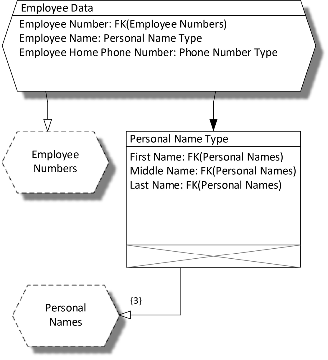
Figure 16-5. A COMN Model for the Employee Data Table

Relational Operations

There are nine relational operators that return relations as results: select (or restrict), join, project, union, intersection, difference, extend, rename, and divide. These relational operators show up directly or indirectly in SQL, and are often present in NoSQL DBMSs as well, of necessity. For instance, an operation that selects documents from a document database based on the value of a particular document element is performing the relational operation of restriction.

Encapsulating data in classes—a common practice in object-oriented programming—disables the relational operators. Relational operators need free access to the data attributes of relations in order to recombine them in useful ways. SQL DBMSs, and other DBMSs that implement the relational operations, provide powerful means to manipulate large quantities of data very efficiently and with minimal programming.

The NoSQL community is in danger of leaving that efficiency and expressiveness behind, and manually replicating the same operations repeatedly at the application level. This is costly and inefficient, and requires that what is (or should be) essentially the same logic be tested over and over. It’s important to be aware that relational theory and relational operations are not tied to SQL or any particular physical implementations, and are best implemented once in a DBMS for all to use.

NoSQL Versus the Relational Model

Relational theory is not about tables; rather, it is about relations, tuples, and types. When we associate relations and tuples with predicates, we add semantics to relational theory.

Most of the time, relations are discussed, just as I have done above, in terms of tables. This leads us to thinking about highly structured and highly repetitive data. But there’s nothing in relational theory that says that a relation has to have many tuple values in it, nor that we can’t have a highly varied set of relations of different schemes, each with one tuple value. So, no matter the context, if you have a data structure of any sort—document, graph, key/value, whatever—where each data attribute has a name that corresponds to its role and a type that limits its possible values, you have a tuple scheme, and relational theory applies. This is true of XML and JSON, even when the typing is so weak as to allow any string of characters to be a value for the data attribute.

What makes NoSQL stand apart from SQL is not that it leaves the relational model behind. It is impossible to leave the relational model behind. It will tag along behind all your data structures. NoSQL is distinctive because its various physical realizations are usually optimized for data exhibiting a great variety of tuple and relation schemes, rather than large sets of data conforming to a small number of schemes. NoSQL is also distinctive because of its more varied approaches to things such as consistency and availability. We’ll explore those in greater depth in the next chapter.

SQL Versus the Relational Model

SQL (Structured Query Language) databases are the best-known representatives of the relational model of data, and relational theory is usually judged by the characteristics of SQL databases, most of which are physical and not related to relational theory directly. We will dig into many of those differences in the next chapter on NoSQL and SQL physical database design. For now, we will focus only on the extent to which SQL is an implementation of the relational model.

A database definition in SQL always starts with a CREATE TABLE statement. There is no CREATE RELATION statement in SQL. It follows from this that the SQL language describes physical tables, which have the characteristics of order and repetition explained above. Now, any physical table, including a SQL table, has order to its rows, and there is no possibility of preventing this. SQL DBMSs do state up front that the order of rows in a table is not necessarily preserved across operations on a table, nor across changes to the DBMS software, so it is impossible to store information in the order of a table’s rows. (Well, almost impossible: I knew of one system that failed because a programmer expected a certain SQL query to return rows from a table in a certain order; when the DBMS software was upgraded, the order changed and the code depending on that order failed. Fortunately, the bug was easily fixed by adding an explicit ORDER BY clause to the SQL query.)

SQL tables allow two or more rows to represent the same values; they therefore allow repetition. With the addition of a PRIMARY KEY or UNIQUE INDEX to a table, a SQL DBMS will prevent this from happening, making a SQL table a true representative of a relation from relational theory.

In other words, unless additional steps are taken, a SQL table can contain two or more rows representing identical values.

Now, there’s nothing wrong with tables as tables, but given that SQL DBMSs do not promise to preserve the order of rows in tables, the only aspect of tables as opposed to relations that remains available for use is the ability to store the same row value more than once. If this can be useful in some application, great, but it’s more likely to be a source of error, where a table allows duplicate data to be stored inadvertently.

But a data design properly executed in COMN will indicate the key data attributes for each logical record type, and this translates directly into SQL as a table with one or more unique indexes, thereby preventing duplicate data and making a table an accurate representation of a relation.

Terminology

Relational Term	COMN Term
attribute	data attribute
(no relational equivalent)	attribute: an inherent characteristic
attribute value	data attribute value
tuple scheme	composite type logical record type if intended to be used as such
tuple variable	a variable having a composite type a logical record if intended to be used as such
tuple, tuple value	value of a composite type
relation scheme	composite type for a collection of logical records
relation variable	a variable having a relation scheme as its type
relation, relation value	value of a relation variable

Key Points The relation of relational theory is not a relationship. This is a great terminological tragedy that has impeded comprehension of relational theory. A relation is like a table where the order of the rows is irrelevant, and any repeated row values are irrelevant. Making order irrelevant enables data independence, so that data can be reordered for faster access. Type nesting is compatible with relational theory, but the lack of support for type nesting in SQL and E-R notations have led to the belief that one must abandon relational theory in order to gain type nesting. Relational operators are powerful means for recombining data in useful ways. Encapsulating data disables these operators, and leaving them out of NoSQL DBMSs forces them to be implemented repeatedly in applications, with resulting higher costs, lower quality, and lower reliability.

Chapter Glossary

attribute : an inherent characteristic (Merriam-Webster)

data attribute : a <name, type> pair. The name gives the role of a value of the given type in the context of a tuple scheme or relation scheme.

data attribute value : a <name, type, value> triple

tuple : a tuple value

tuple value : a set of data attribute values

tuple scheme : the specification of the data attributes of a tuple, together with any constraints referencing a tuple value as a whole

relation : a relation value

relation value : a set of tuple values all having the same tuple scheme; informally, a table without significance to the order of or repetition of the values of its rows

relation scheme : the specification of the data attributes of a relation, together with other information such as keys and other constraints on a relation value as a whole

tuple variable : a symbol which can be bound to a tuple value

relation variable : a symbol which can be bound to a relation value

data independence : the ability to re-order data without losing any information