Introduction to Profiling

In general, JVM profiling and monitoring tools operate by using some low-level instrumentation and either feeding data back to a graphical console or saving it in a log for later analysis. The low-level instrumentation usually takes the form of either an agent loaded at application start or a component that dynamically attaches to a running JVM.

In broad terms, we need to distinguish between monitoring tools (whose primary goal is observing the system and its current state), alerting systems (for detecting abnormal or anomalous behavior), and profilers (which provide deep-dive information about running applications). These tools have different, although often related, objectives and a well-run production application may make use of all of them.

The focus of this chapter, however, is profiling. The aim of (execution) profiling is to identify user-written code that is a target for refactoring and performance optimization.

As discussed in “Basic Detection Strategies”, the first step in diagnosing and correcting a performance problem is to identify which resource is causing the issue. An incorrect identification at this step can prove very costly.

If we perform a profiling analysis on an application that is not being limited by CPU cycles, then it is very easy to be badly misled by the output of the profiler. To expand on the Brian Goetz quote from “Introduction to JMH”, the tools will always produce a number—it’s just not clear that the number has any relevance to the problem being addressed. It is for this reason that we introduced the main types of bias in “Cognitive Biases and Performance Testing” and delayed discussion of profiling techniques until now.

A good programmer…will be wise to look carefully at the critical code; but only after that code has been identified.

Donald Knuth

This means that before undertaking a profiling exercise, performance engineers should have already identified a performance problem. Not only that, but they should also have proved that application code is to blame. They will know this is the case if the application is consuming close to 100% of CPU in user mode.

If these criteria are not met, the engineer should look elsewhere for the source of the problem and should not attempt to diagnose further with an execution profiler.

Even if the CPU is fully maxed out in user mode (not kernel time), there is another possible cause that must be ruled out before profiling: STW phases of GC. As all applications that are serious about performance should be logging GC events, this check is a simple one: consult the GC log and application logs for the machine and ensure that the GC log is quiet and the application log shows activity. If the GC log is the active one, then GC tuning should be the next step—not execution profiling.

Sampling and Safepointing Bias

One key aspect of execution profiling is that it usually uses sampling to obtain data points (stack traces) of what code is running. After all, it is not cost-free to take measurements, so all method entries and exits are not usually tracked in order to prevent an excessive data collection cost. Instead, a snapshot of thread execution is taken—but this can only be done at a relatively low frequency without unacceptable overhead.

For example, the New Relic Thread Profiler (one of the tools available as part of the New Relic stack) will sample every 100 ms. This limit is often considered a best guess on how often samples can be taken without incurring high overhead.

The sampling interval represents a tradeoff for the performance engineer. Sample too frequently and the overhead becomes unacceptable, especially for an application that cares about performance. On the other hand, sample too infrequently and the chance of missing important behavior becomes too large, as the sampling may not reflect the real performance of the application.

By the time you’re using a profiler it should be filling in detail—it shouldn’t be surprising you.

Kirk Pepperdine

Not only does sampling offer opportunities for problems to hide in the data, but in most cases sampling has only been performed at safepoints. This is known as safepointing bias and has two primary consequences:

• All threads must reach a safepoint before a sample can be taken.

• The sample can only be of an application state that is at a safepoint.

The first of these imposes additional overhead on producing a profiling sample from a running process. The second consequence skews the distribution of sample points, by sampling only the state when it is already known to be at a safepoint.

Most execution profilers use the GetCallTrace() function from HotSpot’s C++ API to collect stack samples for each application thread. The usual design is to collect the samples within an agent, and then log the data or perform other downstream processing.

However, GetCallTrace() has a quite severe overhead: if there are N active application threads, then collecting a stack sample will cause the JVM to safepoint N times. This overhead is one of the root causes that set an upper limit on the frequency with which samples can be taken.

The careful performance engineer will therefore keep an eye on how much safepointing time is being used by the application. If too much time is spent in safepointing, then the application performance will suffer, and any tuning exercise may be acting on inaccurate data. A JVM flag that can be very useful for tracking down cases of high safepointing time is:

-XX:+PrintGCApplicationStoppedTime

This will write extra information about safepointing time into the GC log. Some tools (notably jClarity Censum) can automatically detect problems from the data produced by this flag. Censum can also differentiate between safepointing time and pause time imposed by the OS kernel.

One example of the problems caused by safepointing bias can be illustrated by a counted loop. This is a simple loop, of a similar form to this snippet:

for (int i = 0; i < LIMIT; i++) {
    // only "simple" operations in the loop body
}

We have deliberately elided the meaning of a “simple” operation in this example, as the behavior is dependent on the exact optimizations that the JIT compiler can perform. Further relevant details can be found in “Loop Unrolling”.

Examples of simple operations include arithmetic operations on primitives and method calls that have been fully inlined (so that no methods are actually within the body of the loop).

If LIMIT is large, then the JIT compiler will translate this Java code directly into an equivalent compiled form, including a back branch to return to the top of the loop. As discussed in “Safepoints Revisited”, the JIT compiler inserts safepoint checks at loop-back edges. This means that for a large loop, there will be an opportunity to safepoint once per loop iteration.

However, for a small enough LIMIT this will not occur, and instead the JIT compiler will unroll this loop. This means that the thread executing the small-enough counted loop will not safepoint until after the loop has completed.

Only sampling at safepoints has thus led directly to a biasing behavior that is sensitively dependent on the size of the loops and the nature of operations that we perform in them.

This is obviously not ideal for rigorous and reliable performance results. Nor is this a theoretical concern—loop unrolling can generate significant amounts of code, leading to long chunks of code where no samples will ever be collected.

We will return to the problem of safepointing bias, but it remains an excellent example of the kinds of tradeoffs that performance engineers need to be aware of.

Execution Profiling Tools for Developers

In this section we will discuss several different execution profiling tools with graphical UIs. There are quite a few tools available in the market, so we focus on a selection of the most common rather than attempting an exhaustive survey.

VisualVM Profiler

As a first example of a profiling tool, let’s consider VisualVM. It includes both an execution and a memory profiler and is a very straightforward free profiling tool. It is quite limited in that it is rarely usable as a production tool, but it can be helpful to performance engineers who want to understand the behavior of their applications in dev and QA environments.

In Figure 13-1 we can see the execution profiling view of VisualVM.

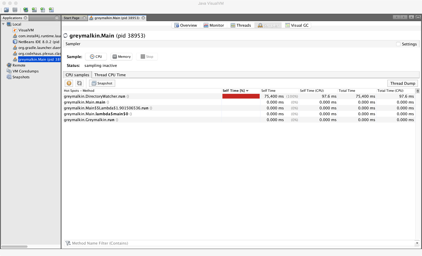
Figure 13-1. VisualVM memory profiler

This shows a simple view of executing methods and their relative CPU consumption. The amount of drilldown that is possible within VisualVM is really quite limited. As a result, most performance engineers quickly outgrow it and turn to one of the more complete tools on the market. However, it can be a useful first tool for performance engineers who are new to the art of and tradeoffs involved in profiling.

JProfiler

One popular commercial profiler is JProfiler from ej-technologies GmbH. This is an agent-based profiler capable of running as a GUI tool as well as in headless mode to profile local or remote applications. It is compatible with a fairly wide range of operating systems, including FreeBSD, Solaris, and AIX, as well as the more usual Windows, macOS, and Linux.

When the desktop application is started for the first time, a screen similar to that shown in Figure 13-2 is displayed.

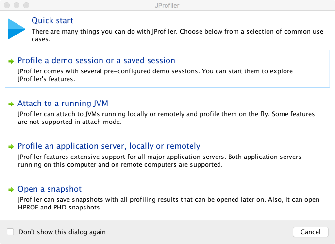
Figure 13-2. JProfiler startup wizard

Clearing this screen gives the default view show in Figure 13-3.

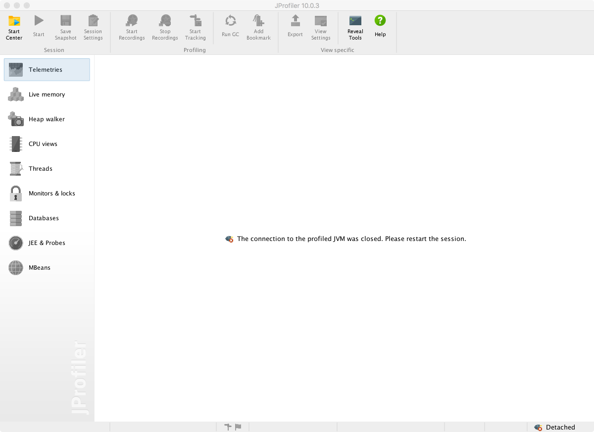
Figure 13-3. JProfiler startup screen

Clicking the Start Center button at the top left gives a variety of options, including Open Session (which contains some precanned examples to work with) and Quick Attach. Figure 13-4 shows the Quick Attach option, where we’re choosing to profile the AsciidocFX application, which is the authoring tool in which much of this book was written.

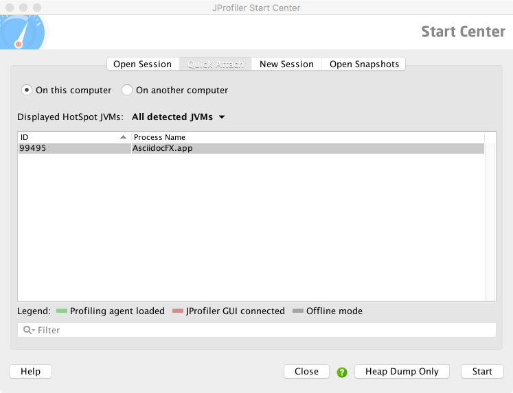
Figure 13-4. JProfiler Quick Attach screen

Attachment to the target JVM brings up a configuration dialog, as shown in Figure 13-5. Note that the profiler is already warning of performance tradeoffs in the configuration of the tool, as well as a need for effective filters and an awareness of the overhead of profiling. As discussed earlier in the chapter, execution profiling is very much not a silver bullet, and the engineer must proceed carefully to avoid confusion.

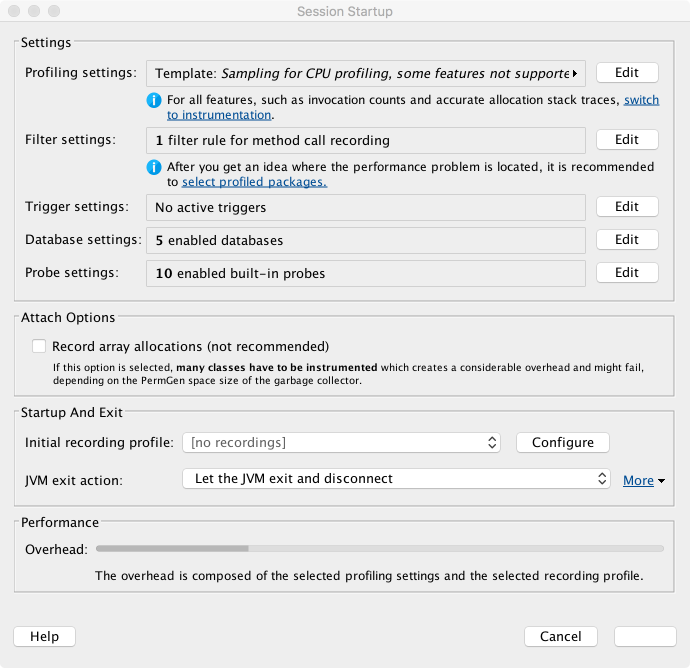
Figure 13-5. JProfiler attach configuration

After an initial scan, JProfiler springs into life. The initial screen shows a telemetry view similar to that of VisualVM, but with a scrolling display rather than the time-resizing view. This view is shown in Figure 13-6.

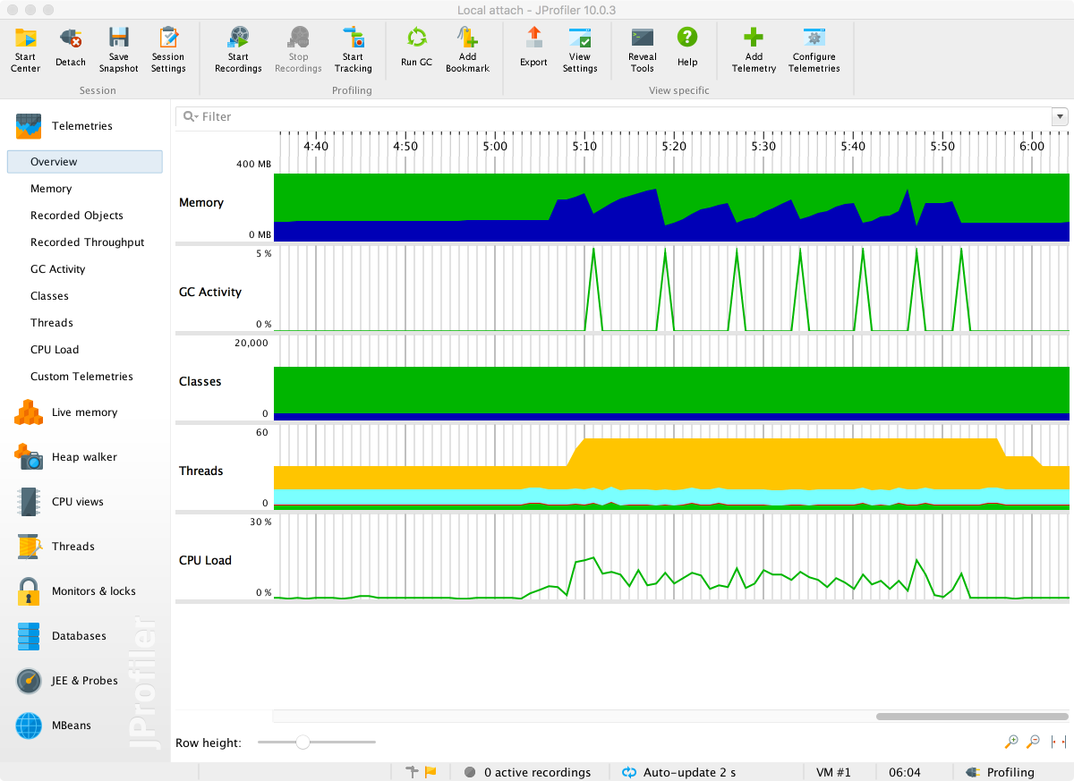
Figure 13-6. JProfiler simple telemetry

From this screen, all the basic views can be accessed, but without switching on some recordings not much can be seen. To see method timings, choose the Call Tree view and press the button to start recording. After a few seconds the results of profiling will start to show up. This should look something like Figure 13-7.

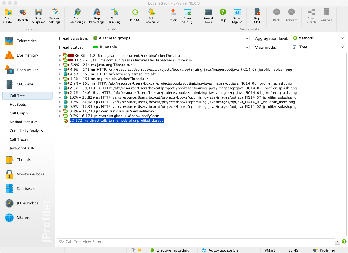
Figure 13-7. JProfiler CPU times

The tree view can be expanded to show the intrinsic time of methods that each method calls.

To use the JProfiler agent, add this switch to the run configuration:

-agentpath:<path-to-agent-lib>

In the default configuration, this will cause the profiled application to pause on startup and wait for a GUI to connect. The intent of this is to front-load the instrumentation of application classes at startup time, so that the application will then run normally.

For the case of production applications, it would not be normal to attach a GUI. In this case the JProfiler agent needs to be added with a configuration that indicates what data to record. These results are only saved to snapshot files to be loaded into the GUI later. JProfiler provides a wizard for configuring remote profiling and appropriate settings to add to the remote JVM.

Finally, the careful reader should note that in the screenshots we are showing the profile of a GUI app that is not CPU-bound, so the results are for demonstration purposes only. The CPU is nowhere near 100% utilized, so this is not a realistic use case for JProfiler (or any other profiling tool).

YourKit

The YourKit profiler is another commercial profiler, produced by YourKit GmbH. The YourKit tool is similar to JProfiler in some ways, offering a GUI component as well as an agent that can either attach dynamically or be configured to run at application start.

To deploy the agent, use the following syntax (for 64-bit Linux):

-agentpath:<profiler-dir>/bin/linux-x86-64/libyjpagent.so

From the GUI perspective, it features similar setup and initial telemetry screens to those seen in VisualVM and JProfiler.

In Figure 13-8 we can see the CPU snapshot view, with drilldown into how the CPU is spending its time. This level of detail goes well beyond what is possible with VisualVM.

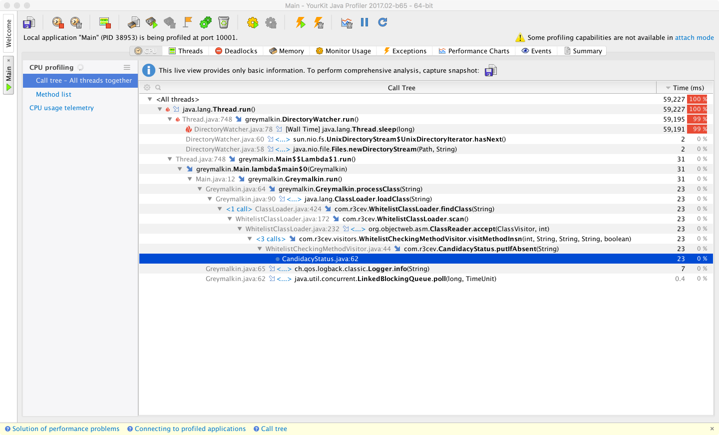
Figure 13-8. YourKit CPU times

In testing, the attach mode of YourKit occasionally displayed some glitches, such as freezing GUI applications. On the whole, though, the execution profiling features of YourKit are broadly on par with those offered by JProfiler; some engineers may simply find one tool more to their personal preference than the other.

If possible, profiling with both YourKit and JProfiler (although not at the same time, as this will introduce extra overhead) may reveal different views of the application that may be useful for diagnosis.

Both tools use the safepointing sampling approach discussed earlier, and so both tools are potentially subject to the same types of limitations and biases induced by this approach.

Flight Recorder and Mission Control

The Java Flight Recorder and Mission Control (JFR/JMC) tools are profiling and monitoring technologies that Oracle obtained as part of its acquisition of BEA Systems. They were previously part of the tooling offering for BEA’s JRockit JVM. The tools were moved to the commercial version of Oracle JDK as part of the process of retiring JRockit.

As of Java 8, Flight Recorder and Mission Control are commercial and proprietary tools. They are available only for the Oracle JVM and will not work with OpenJDK builds or any other JVM.

As JFR is available only for Oracle JDK, you must pass the following switches when starting up an Oracle JVM with Flight Recorder:

-XX:+UnlockCommercialFeatures -XX:+FlightRecorder

In September 2017, Oracle announced a major change to the release schedule of Java, moving it from a two-year release cycle to a six-month cadence. This was the result of the two previous releases (Java 8 and 9) being significantly delayed.

In addition to the decision to change the release cycle, Oracle also announced that post–Java 9, the primary JDK distributed by Oracle would become OpenJDK rather than Oracle JDK. As part of this change, Flight Recorder and Mission Control would become open source tools that are free to use.

At the time of writing, a detailed roadmap for the availability of JFR/JMC as free and open source features has not been announced. Neither has it been announced whether deployments of Java 8 or 9 will need to pay for production usage of JFR/JMC.

Note

The initial installation of JMC consists of a JMX Console and JFR, although more plug-ins can easily be installed from within Mission Control.

JMC is the graphical component, and is started up from the jmc binary in $JAVA_HOME/bin. The startup screen for Mission Control can be seen in Figure 13-9.

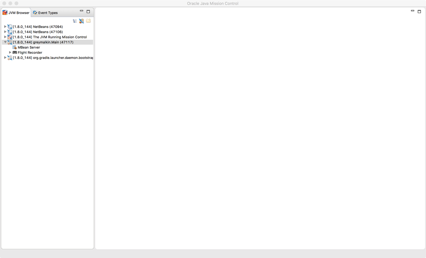
Figure 13-9. JMC startup screen

To profile, Flight Recorder must be enabled on the target application. You can achieve this either by starting with the flags enabled, or by dynamically attaching after the application has already started.

Once attached, enter the configuration for the recording session and the profiling events, as shown in Figures 13-10 and 13-11.

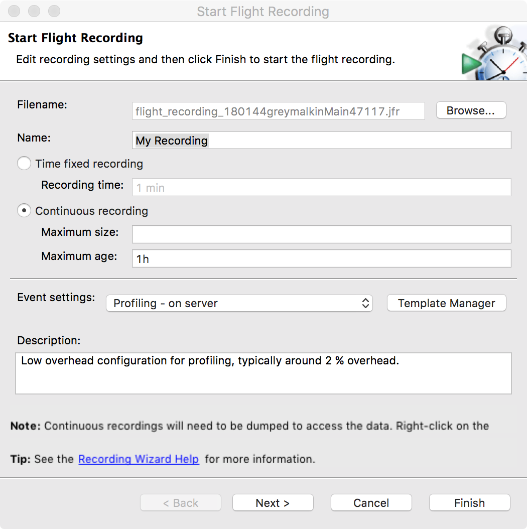
Figure 13-10. JMC recording setup

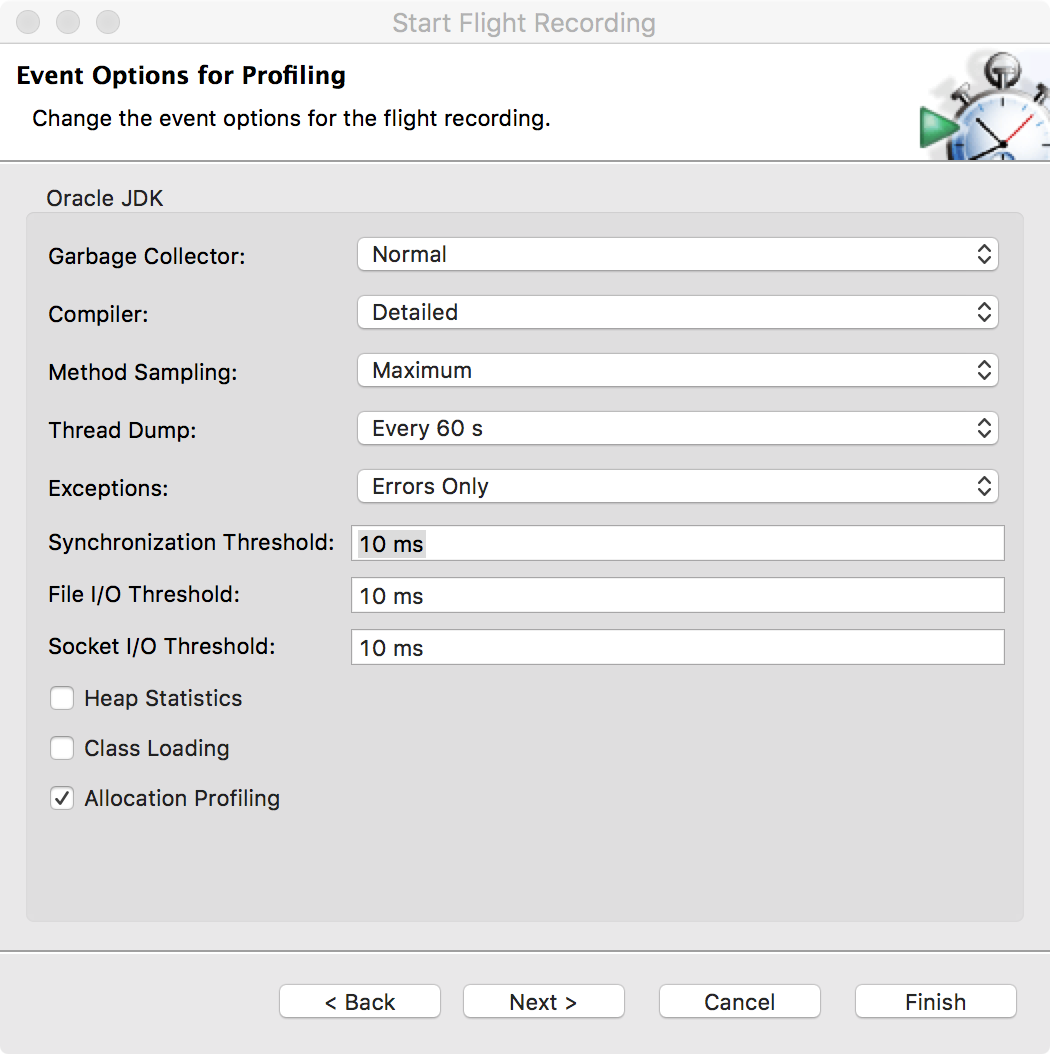
Figure 13-11. JMC profiling event options

When the recording starts, this is typically displayed in a time window, as shown in Figure 13-12.

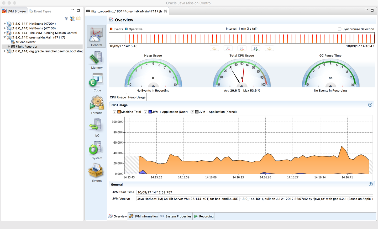
Figure 13-12. JMC time window

To support the port of JFR from JRockit, the HotSpot VM was instrumented to produce a large basket of performance counters similar to those collected in the Serviceability Agent.

Operational Tools

Profilers are, by their nature, developer tools used to diagnose problems or to understand the runtime behavior of applications at a low level. At the other end of the tooling spectrum are operational monitoring tools. These exist to help a team visualize the current state of the system and determine whether the system is operating normally or is anomalous.

This is a huge space, and a full discussion is outside the scope of this book. Instead, we’ll briefly cover three tools in this space, two proprietary and one open source.

Red Hat Thermostat

Thermostat is Red Hat’s open source serviceability and monitoring solution for HotSpot-based JVMs. It is available under the same license as OpenJDK itself, and provides monitoring for both single machines and clusters. It uses MongoDB to store historical data as well as point-in-time capabilities.

Thermostat is designed to be an open, extensible platform and consists of an agent and a client (typically a simple GUI). A simple Thermostat view can be seen in Figure 13-13.

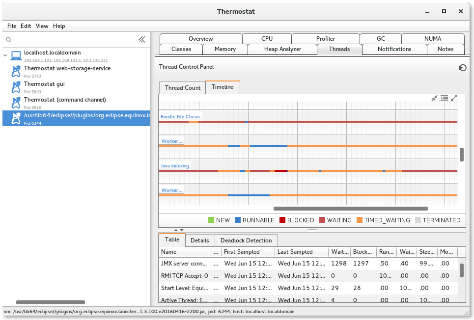
Figure 13-13. Red Hat Thermostat

Thermostat’s architecture allows for extension. For example, you can:

• Collect and analyze your own custom metrics.

• Inject custom code for on-demand instrumentation.

• Write custom plug-ins and integrate tooling.

Most of Thermostat’s built-in functionality is actually implemented as plug-ins.

New Relic

The New Relic tool is a SaaS product designed for cloud-based applications. It is a general-purpose toolset, covering much more than just JVMs.

In the JVM space, installation requires downloading an agent, passing a switch to the JVM, and restarting the server. Following this, New Relic will produce views similar to that shown in Figure 13-14.

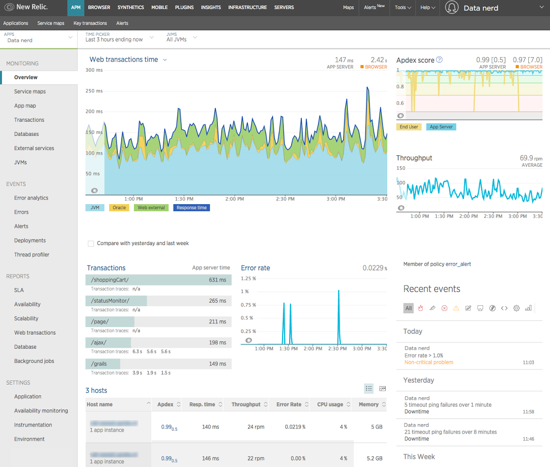
Figure 13-14. New Relic

The general monitoring and full-stack support provided by New Relic can make it an attractive operational and devops tool. However, being a general tool, it has no specific focus on JVM technologies and relies out of the box on the less sophisticated sources of data available from the JVM. This means that for deep-dive information on the JVM, it may need to be combined with more specific tooling.

New Relic provides a Java agent API, or users can implement custom instrumentation to extend its base functionality.

It also suffers from the problem that it generates a huge amount of data, and as a result it can sometimes be difficult to spot anything other than obvious trends in the output.

jClarity Illuminate

A tool that provides a bridge between the developer profiling tools and operational monitoring is jClarity Illuminate. This is not a traditional sampling profiler but instead operates in a monitoring mode with a separate out-of-process daemon that watches the main Java application. If it detects an anomaly in the behavior of the running JVM, such as a service-level agreement (SLA) being breached, Illuminate will initiate a deep-dive probe of the application.

Illuminate’s machine learning algorithm analyzes data collected from the OS, GC logs, and the JVM to determine the root cause of the performance problem. It generates a detailed report and sends it to the user along with some possible next steps to fix the issue. The machine learning algorithm is based on the Performance Diagnostic Model (PDM) originally created by Kirk Pepperdine, one of the founders of jClarity.

In Figure 13-15 we can see the triage mode of Illuminate when it is investigating a problem that has been automatically spotted.

The tool is based on machine learning techniques and is focused on in-depth root-cause analysis, rather than the overwhelming “wall of data” sometimes encountered in monitoring tools. It also drastically reduces the amount of data it needs to collect, move over the network, and store, in an attempt to be a much lower-impact application performance monitoring tool than others in the space.

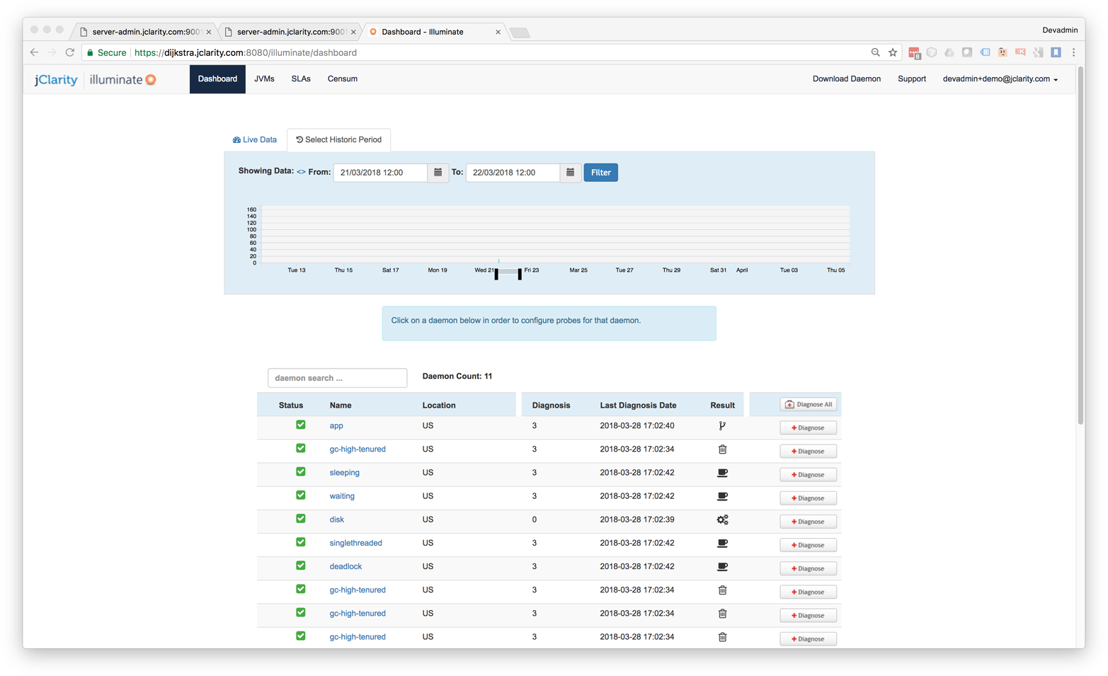
Figure 13-15. jClarity Illuminate

Modern Profilers

In this section we will discuss three modern open source tools that can provide better insight and more accurate performance numbers than traditional profilers. These tools are:

• Honest Profiler

• perf

• Async Profiler

Honest Profiler is a relatively recent arrival to the profiling tool space. It is an open source project led by Richard Warburton, and derives from prototype code written and open-sourced by Jeremy Manson from the Google engineering team.

The key goals of Honest Profiler are to:

• Remove the safepointing bias that most other profilers have.

• Operate with significantly lower overhead.

To achieve this, it makes use of a private API call called AsyncGetCallTrace within HotSpot. This means, of course, that Honest Profiler will not work on a non-OpenJDK JVM. It will work with Oracle, Red Hat, and Azul Zulu JVMs as well as HotSpot JVMs that have been built from scratch.

The implementation uses the Unix OS signal SIGPROF to interrupt a running thread. The call stack can then be collected via the private AsyncGetCallTrace() method.

This only interrupts threads individually, so there is never any kind of global synchronization event. This avoids the contention and overhead typically seen in traditional profilers. Within the asynchronous callback the call trace is written into a lock-free ring buffer. A dedicated separate thread then writes out the details to a log without pausing the application.

Historically, Sun Microsystems also offered the older Solaris Studio product, which also used the private API call. Unfortunately, the name of the product was rather confusing—it actually ran on other operating systems too, not just Solaris—and it failed to gain adoption.

One disadvantage of Honest Profiler is that it may show “Unknown” at the top of some threads. This is a side effect of JVM intrinsics; the profiler is unable to map back to a true Java stack trace correctly in that case.

To use Honest Profiler, the profiler agent must be installed:

-agentpath:<path-to-liblagent.so>=interval=<n>,logPath=<path-to-log.hpl>

Honest Profiler includes a relatively simple GUI for working with profiles. This is based on JavaFX and so will require installation of OpenJFX in order to run on an OpenJDK-based build (such as Azul Zulu or Red Hat IcedTea).

Figure 13-16 shows a typical Honest Profiler GUI screen.

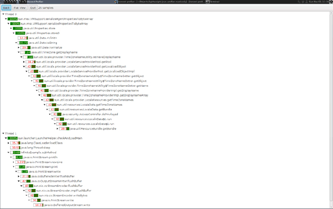
Figure 13-16. Honest Profiler

In practice, tools like Honest Profiler are more commonly run in headless mode as data collection tools. In this approach, visualization is provided by other tooling or custom scripts.

The project does provide binaries, but they are quite limited in scope—only for a recent Linux build. Most serious users of Honest Profiler will need to build their own binary from scratch, a topic which is out of scope for this book.

The perf tool is a useful lightweight profiling solution for applications that run on Linux. It is not specific to Java/JVM applications but instead reads hardware performance counters and is included in the Linux kernel, under tools/perf.

Performance counters are physical registers that count hardware events of interest to performance analysts. These include instructions executed, cache misses, and branch mispredictions. This forms a basis for profiling applications.

Java presents some additional challenges for perf, due to the dynamic nature of the Java runtime environment. To use perf with Java applications, we need a bridge to handle mapping the dynamic parts of Java execution.

This bridge is perf-map-agent, an agent that will generate dynamic symbols for perf from unknown memory regions (including JIT-compiled methods). Due to HotSpot’s dynamically created interpreter and jump tables for virtual dispatch, these must also have entries generated.

perf-map-agent consists of an agent written in C and a small Java bootstrap that attaches the agent to a running Java process if needed. In Java 8u60 a new flag was added to enable better interaction with perf:

-XX:+PreserveFramePointer

When using perf to profile Java applications, it is strongly advised that you are running on 8u60 or later, to give access to this flag.

One striking visualization of the numbers perf produces is the flame graph. This shows a highly detailed breakdown of exactly where execution time is being spent. An example can be seen in Figure 13-17.

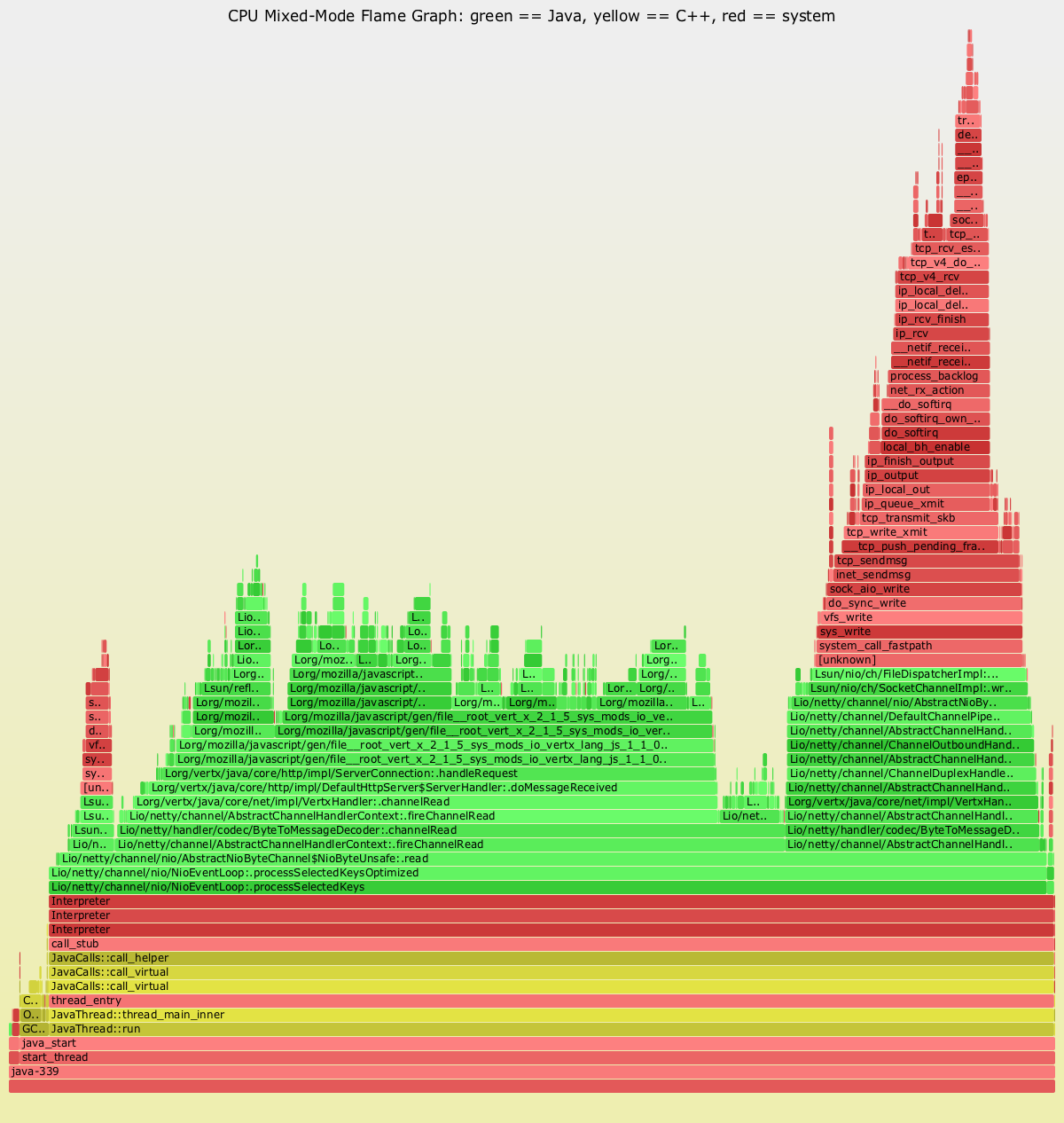
Figure 13-17. Java flame graph

The Netflix Technology Blog has some detailed coverage of how the team has implemented flame graphs on its JVMs.

Finally, an alternative choice to Honest Profiler is Async Profiler. It uses the same internal API as Honest Profiler, and is an open source tool that runs only on HotSpot JVMs. Its reliance on perf means that Async Profiler also works only on the operating systems where perf works (primarily Linux).

Allocation Profiling

Execution profiling is an important aspect of profiling—but it is not the only one! Most applications will also require some level of memory profiling, and one standard approach is to consider the allocation behavior of the application. There are several possible approaches to allocation profiling.

For example, we could use the HeapVisitor approach that tools like jmap rely upon. In Figure 13-18 we can see the memory profiling view of VisualVM, which uses this simple approach.

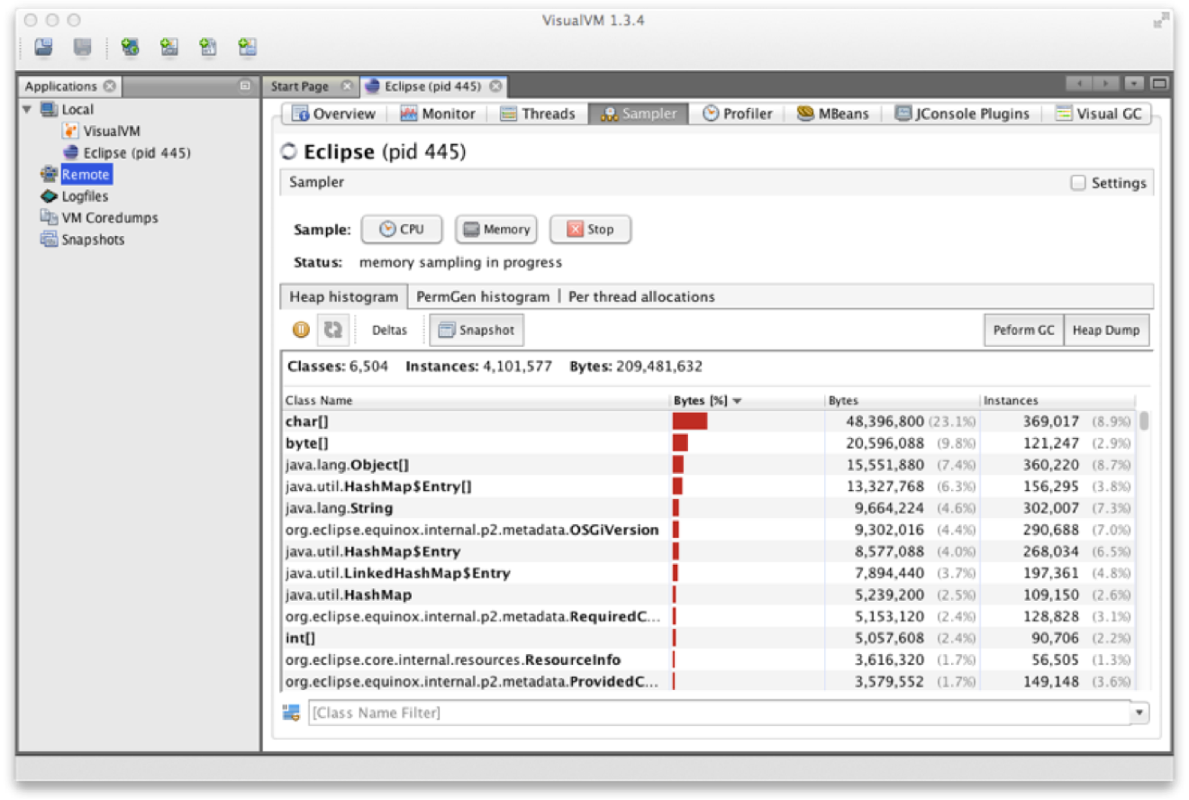
Figure 13-18. VisualVM memory profiler

A similar view can be seen in Figure 13-19, where we show the same capability using the YourKit allocation profiler.

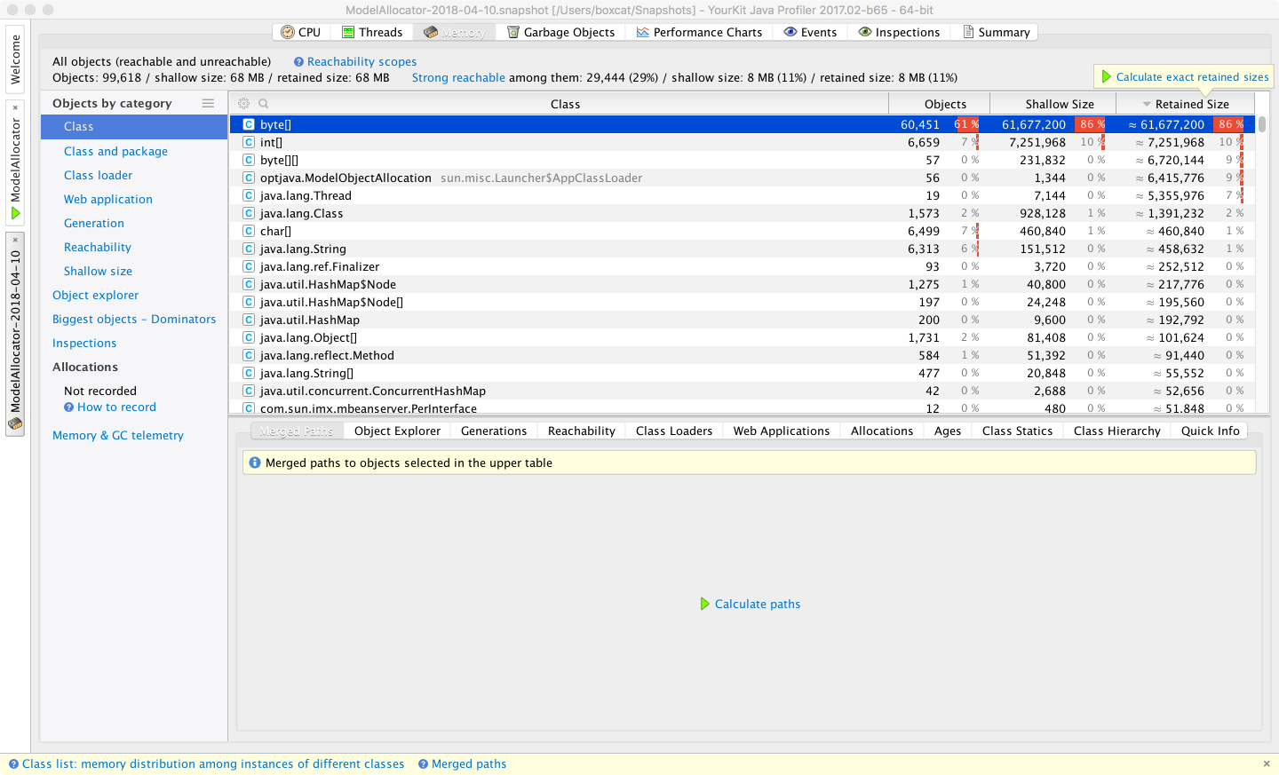
Figure 13-19. YourKit memory profiler

For the JMC tool, the garbage collection statistics contain some values not available in the traditional Serviceability Agent. However, the vast majority of counters presented are duplicates. The advantage is that the cost for JFR to collect these values so they can be displayed in JMC is much cheaper than it is with the SA. The JMC displays also provide greater flexibility to the performance engineer in terms of how the details are displayed.

Another approach to allocation profiling is agent-based profiling. This can be done in several ways, one of the simplest of which is to instrument the bytecode. As seen in “Introduction to JVM Bytecode”, there are three bytecodes that instruct the JVM to allocate memory:

NEW

Allocates space for a new object of a specified type

NEWARRAY

Allocates space for an array of primitives

ANEWARRAY

Allocates space for an array of objects of a specified type

These are the only bytecodes that need to be instrumented, as they are the only opcodes that can cause allocation to occur.

A simple instrumentation approach would consist of locating every instance of any of the allocation opcodes and inserting a call to a static method that logs the allocation before the allocation opcode executes.

Let’s look at the skeleton of such an allocation profiler. We will need to set up the agent using the instrumentation API via a premain() hook:

public class AllocAgent {

    public static void premain(String args, Instrumentation instrumentation) {
        AllocRewriter transformer = new AllocRewriter();
        instrumentation.addTransformer(transformer);
    }

}

To perform this sort of bytecode instrumentation it is usual to use a library, rather than trying to perform the transformations with hand-rolled code. One common bytecode manipulation library in wide use is ASM, which we will use to demonstrate allocation profiling.

To add the required allocation instrumentation code, we need a class rewriter. This provides the bridge between the instrumentation API and ASM and looks like this:

public class AllocRewriter implements ClassFileTransformer {

    @Override
    public byte[] transform(ClassLoader loader, String className,
      Class<?> classBeingRedefined, ProtectionDomain protectionDomain,
      byte[] originalClassContents) throws IllegalClassFormatException {
        final ClassReader reader = new ClassReader(originalClassContents);
        final ClassWriter writer = new ClassWriter(reader,
            ClassWriter.COMPUTE_FRAMES | ClassWriter.COMPUTE_MAXS);
        final ClassVisitor coster = new ClassVisitor(Opcodes.ASM5, writer) {
            @Override
            public MethodVisitor visitMethod(final int access, final String name,
                final String desc, final String signature,
                final String[] exceptions) {
                final MethodVisitor baseMethodVisitor =
                    super.visitMethod(access, name, desc, signature, exceptions);
                return new AllocationRecordingMethodVisitor(baseMethodVisitor,
                    access, name, desc);
            }
        };
        reader.accept(coster, ClassReader.EXPAND_FRAMES);
        return writer.toByteArray();
    }

}

This uses a method visitor to inspect the bytecode and insert instrumentation calls to allow the allocation to be tracked:

public final class AllocationRecordingMethodVisitor extends GeneratorAdapter {
    private final String runtimeAccounterTypeName =
        "optjava/bc/RuntimeCostAccounter";

    public AllocationRecordingMethodVisitor(MethodVisitor methodVisitor,
        int access, String name, String desc) {
        super(Opcodes.ASM5, methodVisitor, access, name, desc);
    }

    /**
     * This method is called when visiting an opcode with a single int operand.
     * For our purposes this is a NEWARRAY opcode.
     *
     * @param opcode
     * @param operand
     */
    @Override
    public void visitIntInsn(final int opcode, final int operand) {
        if (opcode != Opcodes.NEWARRAY) {
            super.visitIntInsn(opcode, operand);
            return;
        }

        // Opcode is NEWARRAY - recordArrayAllocation:(Ljava/lang/String;I)V
        // Operand value should be one of Opcodes.T_BOOLEAN,
        // Opcodes.T_CHAR, Opcodes.T_FLOAT, Opcodes.T_DOUBLE, Opcodes.T_BYTE,
        // Opcodes.T_SHORT, Opcodes.T_INT or Opcodes.T_LONG.
        final int typeSize;
        switch (operand) {
            case Opcodes.T_BOOLEAN:
            case Opcodes.T_BYTE:
                typeSize = 1;
                break;
            case Opcodes.T_SHORT:
            case Opcodes.T_CHAR:
                typeSize = 2;
                break;
            case Opcodes.T_INT:
            case Opcodes.T_FLOAT:
                typeSize = 4;
                break;
            case Opcodes.T_LONG:
            case Opcodes.T_DOUBLE:
                typeSize = 8;
                break;
            default:
                throw new IllegalStateException("Illegal op: to NEWARRAY seen: "
                    + operand);
        }
        super.visitInsn(Opcodes.DUP);
        super.visitLdcInsn(typeSize);
        super.visitMethodInsn(Opcodes.INVOKESTATIC, runtimeAccounterTypeName,
            "recordArrayAllocation", "(II)V", true);
        super.visitIntInsn(opcode, operand);
    }

    /**
     * This method is called when visiting an opcode with a single operand, that
     * is a type (represented here as a String).
     *
     * For our purposes this is either a NEW opcode or an ANEWARRAY.
     *
     * @param opcode
     * @param type
     */
    @Override
    public void visitTypeInsn(final int opcode, final String type) {
        // opcode is either NEW - recordAllocation:(Ljava/lang/String;)V
        // or ANEWARRAY - recordArrayAllocation:(Ljava/lang/String;I)V
        switch (opcode) {
            case Opcodes.NEW:
                super.visitLdcInsn(type);
                super.visitMethodInsn(Opcodes.INVOKESTATIC,
                    runtimeAccounterTypeName, "recordAllocation",
                    "(Ljava/lang/String;)V", true);
                break;
            case Opcodes.ANEWARRAY:
                super.visitInsn(Opcodes.DUP);
                super.visitLdcInsn(8);
                super.visitMethodInsn(Opcodes.INVOKESTATIC,
                runtimeAccounterTypeName, "recordArrayAllocation",
                    "(II)V", true);
                break;
        }

        super.visitTypeInsn(opcode, type);
    }
}

This would also require a small runtime component:

public class RuntimeCostAccounter {
    private static final ThreadLocal<Long> allocationCost =
        new ThreadLocal<Long>() {
        @Override
        protected Long initialValue() {
            return 0L;
        }
    };

    public static void recordAllocation(final String typeName) {
        // More sophistication clearly necessary
        // E.g. caching approximate sizes for types that we encounter
        checkAllocationCost(1);
    }

    public static void recordArrayAllocation(final int length,
        final int multiplier) {
        checkAllocationCost(length * multiplier);
    }

    private static void checkAllocationCost(final long additional) {
        final long newValue = additional + allocationCost.get();
        allocationCost.set(newValue);
        // Take action? E.g. failing if some threshold has been exceeded.
    }

    // This could be exposed, e.g. via a JMX counter
    public static long getAllocationCost() {
        return allocationCost.get();
    }

    public static void resetCounters() {
        allocationCost.set(0L);
    }
}

The aim of these two pieces is to provide simple allocation instrumentation. They use the ASM bytecode manipulation library (a full description of which is unfortunately outside the scope of this book). The method visitor adds in a call to a recording method prior to each instance of the bytecodes NEW, NEWARRAY, and ANEWARRAY.

With this transformation in place, whenever any new object or array is created, the recording method is called. This must be supported at runtime by a small class, the RuntimeCostAccounter (which must be on the classpath). This class maintains per-thread counts of how much memory has been allocated in the instrumented code.

This bytecode-level technique is rather crude, but it should provide a starting point for interested readers to develop their own simple measurements of how much memory is being allocated by their threads. For example, this could be used in a unit or regression test to ensure that changes to the code are not introducing large amounts of extra allocation.

However, for full production usage this approach may not be suitable. There are additional method calls occurring every time memory is allocated, leading to a huge amount of extra calls. JIT compilation will help, as the instrumented calls will be inlined, but the overall effect is likely to have a highly significant effect on performance.

Another approach to allocation profiling is TLAB exhaustion. For example, Async Profiler features TLAB-driven sampling. This uses HotSpot-specific callbacks to receive notifications:

• When an object is allocated in a newly created fresh TLAB

• When an object is allocated outside of a TLAB (the “slow path”)

As a result, not every object allocation is counted. Instead, in aggregate, allocations every n KB are recorded, where n is the average size of the TLAB (recall that the size of a TLAB can change over time).

This design aims to make heap sampling cheap enough to be suitable for production. On the other hand, the collected data has been sampled and so may not be complete. The intent is that in practice it will reflect the top allocation sources, at least enough of the time to be useful to the performance engineer.

To use the TLAB sampling feature, a HotSpot JVM with version 7u40 or later is required, because this version is where the TLAB callbacks first appeared.

Heap Dump Analysis

A technique related to allocation profiling is heap dump analysis. This is the use of tool to examine a snapshot of an entire heap and determine salient facts, such as the live set and numbers and types of objects, as well as the shape and structure of the object graph.

With a heap dump loaded, performance engineers can then traverse and analyze the snapshot of the heap at the time the heap dump was created. They will be able to see live objects and any objects that have died but not yet been collected.

The primary drawback of heap dumps is their sheer size. A heap dump can frequently be 300–400% the size of the memory being dumped. For a multigigabyte heap this is substantial. Not only must the heap be written to disk, but for a real production use case, it must be retrieved over the network as well. Once retrieved, it must then be loaded on a workstation with sufficient resources (especially memory) to handle the dump without introducing excessive delays to the workflow. Working with large heap dumps on a machine that can’t load the whole dump at once can be very painful, as the workstation pages parts of the dump file on and off disk.

Production of a heap file also requires an STW event while the heap is traversed and the dump written out.

YourKit supports capturing memory snapshots in both hprof and a proprietary format. Figure 13-20 shows a view of the heap dump analyzer.

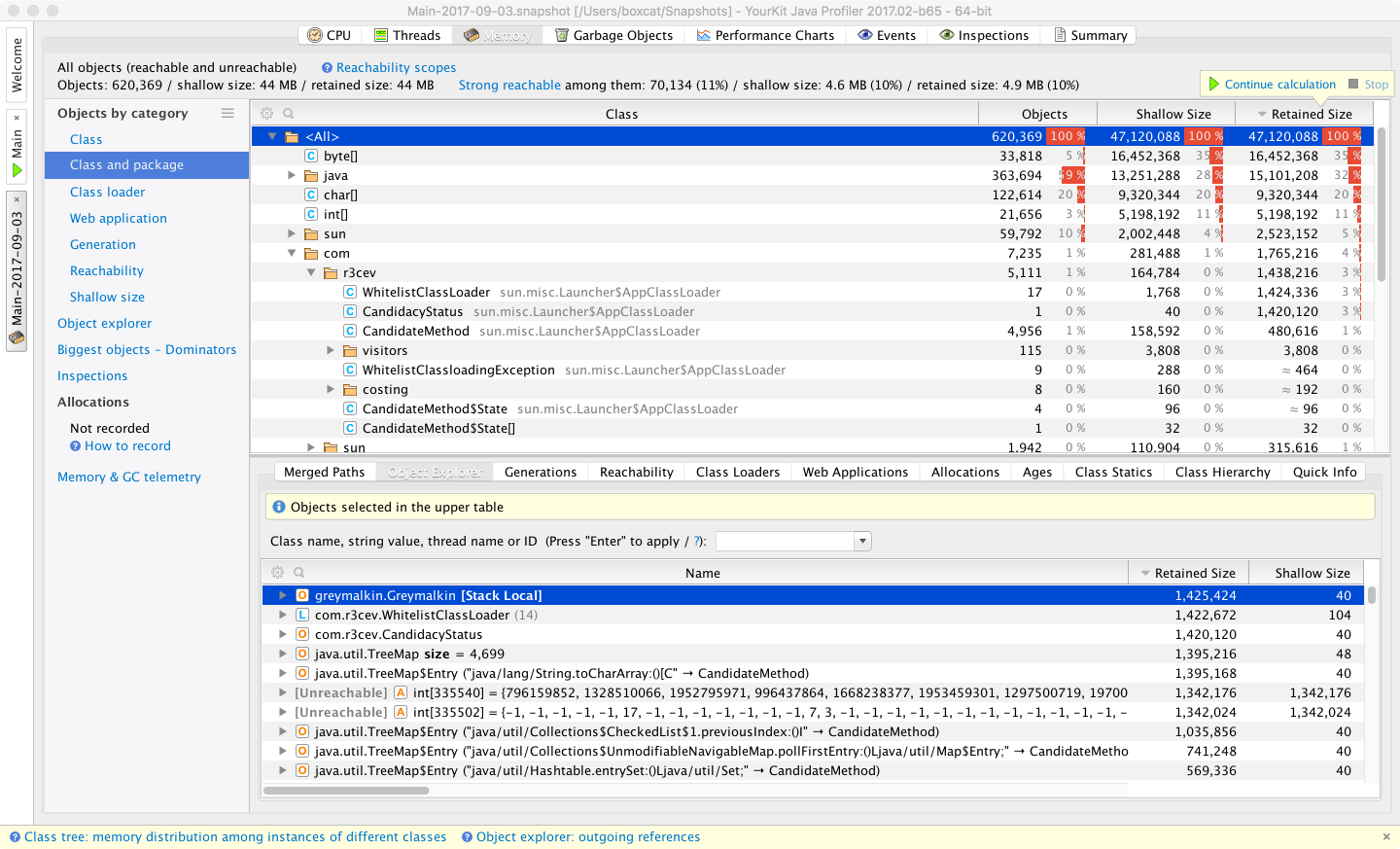
Figure 13-20. YourKit memory dump profiler

Among the commercial tools, YourKit provides a good selection of filters and other views of a heap dump. This includes being able to break it down by classloader and web app, which can lead to faster diagnosis of heap problems.

The Allocations view of JMC/JFR is also worth considering as a tool. It is capable of displaying the TLAB allocation view that is also used by Async Profiler. Figure 13-21 shows a sample image of JMC’s view of allocations.

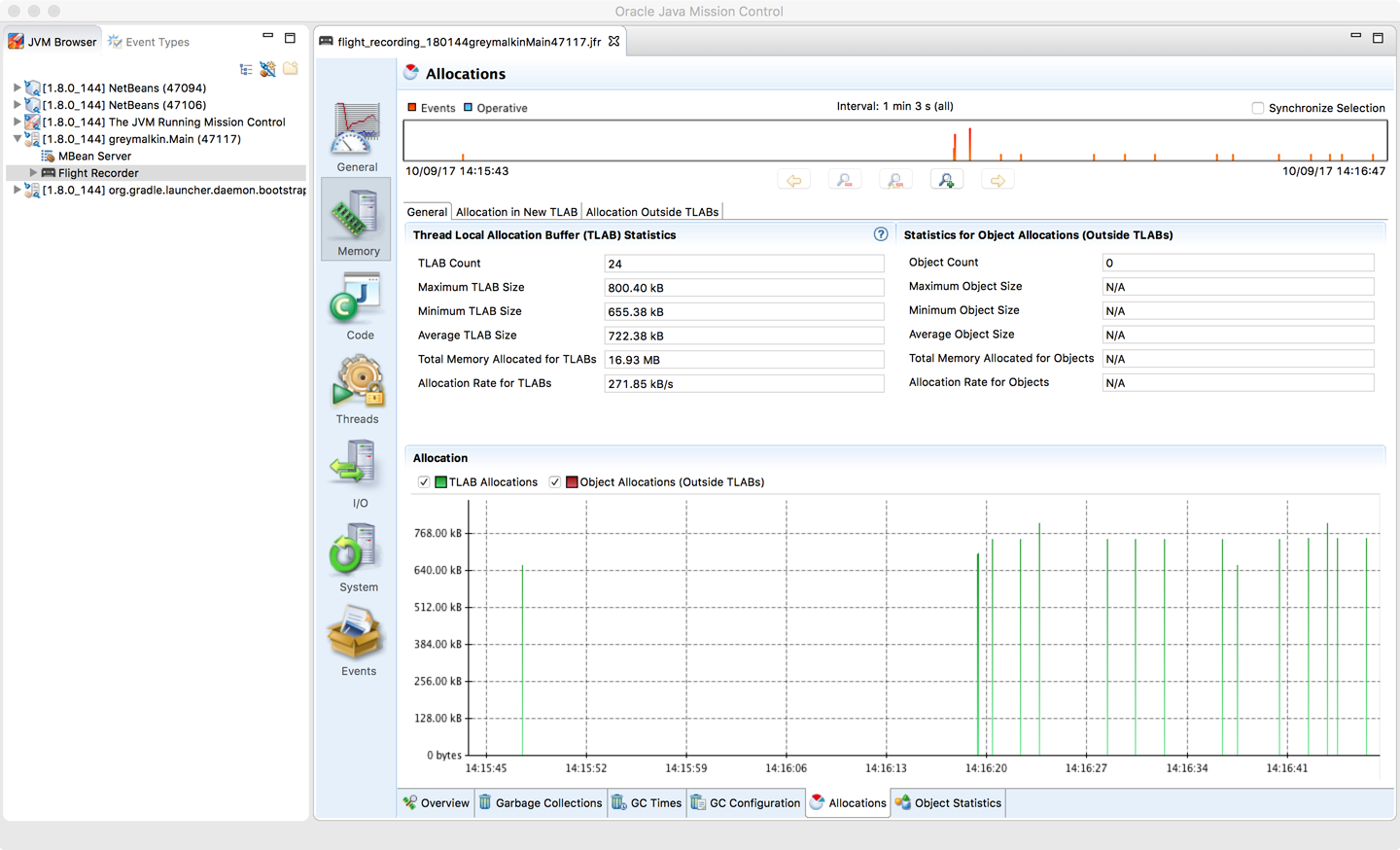
Figure 13-21. JMC Allocations profiling view

Allocation and heap profiling are of interest for the majority of applications that need to be profiled, and performance engineers are encouraged not to overfocus on execution profiling at the expense of memory.

Summary

The subject of profiling is one that is often misunderstood by developers. Both execution and memory profiling are necessary techniques. However, it is very important that performance engineers understand what they are doing, and why. Simply using the tools blindly can produce completely inaccurate or irrelevant results and waste a lot of analysis time.

Profiling modern applications requires the use of tooling, and there are a wealth of options to choose from, including both commercial and open source options.