Table of Contents for
Optimizing Java
 Optimizing Java
Published by
O'Reilly Media, Inc., 2018
Optimizing Java
Published by
O'Reilly Media, Inc., 2018
- nav
- Cover
- Optimizing Java
- Optimizing Java
- Dedication
- Foreword
- Preface
- 1. Optimization and Performance Defined
- 2. Overview of the JVM
- 3. Hardware and Operating Systems
- 4. Performance Testing Patterns and Antipatterns
- 5. Microbenchmarking and Statistics
- 6. Understanding Garbage Collection
- 7. Advanced Garbage Collection
- 8. GC Logging, Monitoring, Tuning, and Tools
- 9. Code Execution on the JVM
- 10. Understanding JIT Compilation
- 11. Java Language Performance Techniques
- 12. Concurrent Performance Techniques
- 13. Profiling
- 14. High-Performance Logging and Messaging
- 15. Java 9 and the Future
- Index
- About the Authors
- Colophon
Chapter 9. Code Execution on the JVM
The two main services that any JVM provides are memory management and an easy-to-use container for execution of application code. We covered garbage collection in some depth in Chapters 6 through 8, and in this chapter we turn to code execution.
Note
Recall that the Java Virtual Machine specification, usually referred to as the VMSpec, describes how a conforming Java implementation needs to execute code.
The VMSpec defines execution of Java bytecode in terms of an interpreter. However, broadly speaking, interpreted environments have unfavorable performance as compared to programming environments that execute machine code directly. Most production-grade modern Java environments solve this problem by providing dynamic compilation capability.
As we discussed in Chapter 2, this ability is otherwise known as Just-in-Time compilation, or just JIT compilation. It is a mechanism by which the JVM monitors which methods are being executed in order to determine whether individual methods are eligible for compilation to directly executable code.
In this chapter we start by providing a brief overview of bytecode interpretation and why HotSpot is different from other interpreters that you may be familiar with. We then turn to the basic concepts of profile-guided optimization. We discuss the code cache and then introduce the basics of HotSpot’s compilation subsystem.
In the following chapter we will explain the mechanics behind some of HotSpot’s most common optimizations, how they are used to produce very fast compiled methods, to what extent they can be tuned, and also their limitations.
Overview of Bytecode Interpretation
As we saw briefly in “Interpreting and Classloading”, the JVM interpreter operates as a stack machine. This means that, unlike with physical CPUs, there are no registers that are used as immediate holding areas for computation. Instead, all values that are to be operated on are placed on an evaluation stack and the stack machine instructions work by transforming the value(s) at the top of the stack.
The JVM provides three primary areas to hold data:
-
The evaluation stack, which is local to a particular method
-
Local variables to temporarily store results (also local to methods)
-
The object heap, which is shared between methods and between threads
A series of VM operations that use the evaluation stack to perform computation can be seen in Figures 9-1 through 9-5, as a form of pseudocode that should be instantly recognizable to Java programmers.
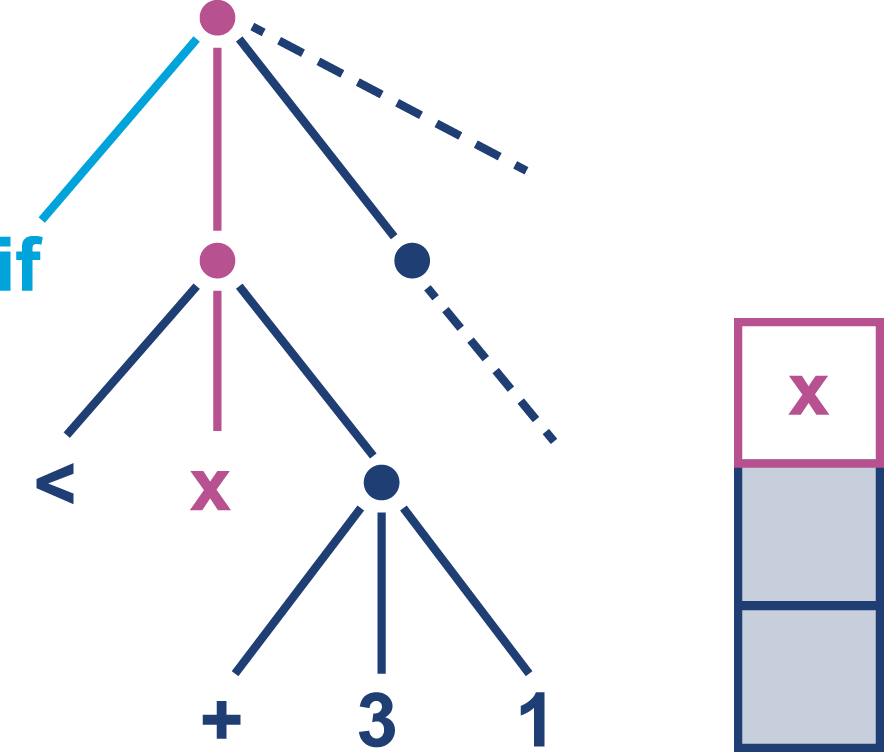
Figure 9-1. Initial interpretation state
The interpreter must now compute the righthand subtree to determine a value to compare with the contents of x.
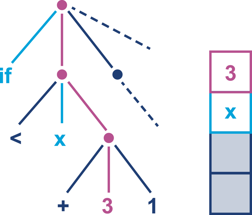
Figure 9-2. Subtree evaluation
The first value of the next subtree, an int constant 3, is loaded onto the stack.
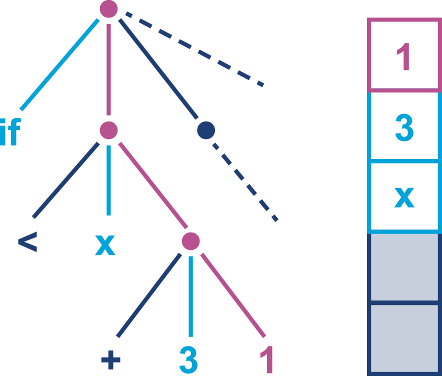
Figure 9-3. Subtree evaluation
Now another int value, 1, is also loaded onto the stack. In a real JVM these values will have been loaded from the constants area of the class file.
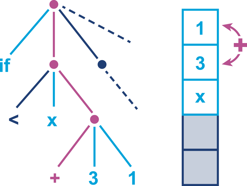
Figure 9-4. Subtree evaluation
At this point, the addition operation acts on the top two elements of the stack, removes them, and replaces them with the result of adding the two numbers together.
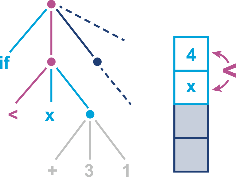
Figure 9-5. Final subtree evaluation
The resulting value is now available for comparison with the value contained in x, which has remained on the evaluation stack throughout the entire process of evaluating the other subtree.
Introduction to JVM Bytecode
In the case of the JVM, each stack machine operation code (opcode) is represented by 1 byte, hence the name bytecode. Accordingly, opcodes run from 0 to 255, of which roughly 200 are in use as of Java 10.
Bytecode instructions are typed, in the sense that iadd and dadd expect to find the correct primitive types (two int and two double values, respectively) at the top two positions of the stack.
Note
Many bytecode instructions come in “families,” with as many as one instruction for each primitive type and one for object references.
For example, within the store family, specific instructions have specific meanings: dstore means “store the top of stack into a local variable of type double,” whereas astore means “store the top of stack into a local variable of reference type.” In both cases the type of the local variable must match the type of the incoming value.
As Java was designed to be highly portable, the JVM specification was designed to be able to run the same bytecode without modification on both big-endian and little-endian hardware architectures. As a result, JVM bytecode has to make a decision about which endianness convention to follow (with the understanding that hardware with the opposite convention must handle the difference in software).
Tip
Bytecode is big-endian, so the most significant byte of any multi-byte sequence comes first.
Some opcode families, such as load, have shortcut forms. This allows the argument to be omitted, which saves the cost of the argument bytes in the class file. In particular, aload_0 puts the current object (i.e., this) on the top of the stack. As that is such a common operation, this results in a considerable savings in class file size.
However, as Java classes are typically fairly compact, this design decision was probably more important in the early days of the platform, when class files—often applets—would be downloaded over a 14.4 Kbps modem.
Note
Since Java 1.0, only one new bytecode opcode (invokedynamic) has been introduced, and two (jsr and ret) have been deprecated.
The use of shortcut forms and type-specific instructions greatly inflates the number of opcodes that are needed, as several are used to represent the same conceptual operation. The number of assigned opcodes is thus much larger than the number of basic operations that bytecode represents, and bytecode is actually conceptually very simple.
Let’s meet some of the main bytecode categories, arranged by opcode family.
Note that in the tables that follow, c1 indicates a 2-byte constant pool index, whereas i1 indicates a local variable in the current method.
The parentheses indicate that the family has some opcodes that are shortcut forms.
The first category we’ll meet is the load and store category, depicted in Table 9-1. This category comprises the opcodes that move data on and off the stack—for example, by loading it from the constant pool or by storing the top of stack into a field of an object in the heap.
| Family name | Arguments | Description |
|---|---|---|
|
( |
Loads value from local variable |
|
( |
Stores top of stack into local variable |
|
|
Loads value from CP#c1 onto the stack |
|
Loads simple constant value onto the stack |
|
|
Discards value on top of stack |
|
|
Duplicates value on top of stack |
|
|
|
Loads value from field indicated by CP#c1 in object on top of stack onto the stack |
|
|
Stores value from top of stack into field indicated by CP#c1 |
|
|
Loads value from static field indicated by CP#c1 onto the stack |
|
|
Stores value from top of stack into static field indicated by CP#c1 |
The difference between ldc and const should be made clear. The ldc bytecode loads a constant from the constant pool of the current class. This holds strings, primitive constants, class literals, and other (internal) constants needed for the program to run.1
The const opcodes, on the other hand, take no parameters and are concerned with loading a finite number of true constants, such as aconst_null, dconst_0, and iconst_m1 (the latter of which loads -1 as an int).
The next category, the arithmetic bytecodes, apply only to primitive types, and none of them take arguments, as they represent purely stack-based operations. This simple category is shown in Table 9-2.
| Family name | Description |
|---|---|
|
Adds two values from top of stack |
|
Subtracts two values from top of stack |
|
Divides two values from top of stack |
|
Multiplies two values from top of stack |
( |
Casts value at top of stack to a different primitive type |
|
Negates value at top of stack |
|
Computes remainder (integer division) of top two values on stack |
In Table 9-3, we can see the flow control category.
This category represents the bytecode-level representation of the looping and branching constructs of source-level languages.
For example, Java’s for, if, while, and switch statements will all be transformed into flow control opcodes after source code compilation.
| Family name | Arguments | Description |
|---|---|---|
|
( |
Branch to the location indicated by the
argument, if the condition is |
|
|
Unconditional branch to the supplied offset |
|
Out of scope |
|
|
Out of scope |
Note
A detailed description of how tableswitch and lookupswitch operate is outside the scope of this book.
The flow control category seems very small, but the true count of flow control opcodes is surprisingly large.
This is due to there being a large number of members of the if opcode family.
We met the if_icmpge opcode (if-integer-compare-greater-or-equal) in the javap example back in Chapter 2, but there are many others that represent different variations of the Java if statement.
The deprecated jsr and ret bytecodes, which have not been output by javac since Java 6, are also part of this family.
They are no longer legal for modern versions of the platform, and so have not been included in this table.
One of the most important categories of opcodes is shown in Table 9-4. This is the method invocation category, and is the only mechanism that the Java program allows to transfer control to a new method. That is, the platform separates completely between local flow control and transfer of control to another method.
| Opcode name | Arguments | Description |
|---|---|---|
|
|
Invokes the method found at CP#c1 via virtual dispatch |
|
|
Invokes the method found at CP#c1 via “special” (i.e., exact) dispatch |
|
|
Invokes the interface method found at CP#c1 using interface offset lookup |
|
|
Invokes the static method found at CP#c1 |
|
|
Dynamically looks up which method to invoke and executes it |
The JVM’s design—and use of explicit method call opcodes—means that there is no equivalent of a call operation as found in machine code.
Instead, JVM bytecode uses some specialist terminology; we speak of a call site, which is a place within a method (the caller) where another method (the callee) is called. Not only that, but in the case of a nonstatic method call, there is always some object that we resolve the method upon. This object is known as the receiver object and its runtime type is referred to as the receiver type.
Note
Calls to static methods are always turned into invokestatic and have no receiver object.
Java programmers who are new to looking at the VM level may be surprised to learn that method calls on Java objects are actually transformed into one of three possible bytecodes (invokevirtual, invokespecial, or invokeinterface), depending on the context of the call.
Tip
It can be a very useful exercise to write some Java code and see what circumstances produce each possibility, by disassembling a simple Java class with javap.
Instance method calls are normally turned into invokevirtual instructions, except when the static type of a receiver object is only known to be an interface type.
In this case, the call is instead represented by an invokeinterface opcode.
Finally, in the cases (e.g., private methods or superclass calls) where the exact method for dispatch is known at compile time, an invokespecial instruction is produced.
This begs the question of how invokedynamic enters the picture.
The short answer is that there is no direct language-level support for invokedynamic in Java, even as of version 10.
In fact, when invokedynamic was added to the runtime in Java 7, there was no way at all to force javac to emit the new bytecode.
In this old version of Java, the invokedynamic technology had only been added to support long-term experimentation and non-Java dynamic languages (especially JRuby).
However, from Java 8 onward, invokedynamic has become a crucial part of the Java language and it is used to provide support for advanced language features.
Let’s take a look at a simple example from Java 8 lambdas:
publicclassLambdaExample{privatestaticfinalStringHELLO="Hello";publicstaticvoidmain(String[]args)throwsException{Runnabler=()->System.out.println(HELLO);Threadt=newThread(r);t.start();t.join();}}
This trivial usage of a lambda expression produces bytecode as shown:
publicstaticvoidmain(java.lang.String[])throwsjava.lang.Exception;Code:0:invokedynamic#2,0// InvokeDynamic #0:run:()Ljava/lang/Runnable;5:astore_16:new#3// class java/lang/Thread9:dup10:aload_111:invokespecial#4// Method java/lang/Thread.// "<init>":(Ljava/lang/Runnable;)V14:astore_215:aload_216:invokevirtual#5// Method java/lang/Thread.start:()V19:aload_220:invokevirtual#6// Method java/lang/Thread.join:()V23:return
Even if we know nothing else about it, the form of the invokedynamic instruction indicates that some method is being called, and the return value of that call is placed upon the stack.
Digging further into the bytecode we discover that, unsurprisingly, this value is the object reference corresponding to the lambda expression.
It is created by a platform factory method that is being called by the invokedynamic instruction.
This invocation makes reference to extended entries in the constant pool of the class to support the dynamic runtime nature of the call.
This is perhaps the most obvious use case of invokedynamic for Java programmers, but it is not the only one.
This opcode is extensively used by non-Java languages on the JVM, such as JRuby and Nashorn (JavaScript), and increasingly by Java frameworks as well.
However, for the most part it remains something of a curiosity, albeit one that a performance engineer should be aware of.
We will meet some related aspects of invokedynamic later in the book.
The final category of opcodes we’ll consider are the platform opcodes. They are shown in Table 9-5, and comprise operations such as allocating new heap storage and manipulating the intrinsic locks (the monitors used by synchronization) on individual objects.
| Opcode name | Arguments | Description |
|---|---|---|
|
|
Allocates space for an object of type found at CP#c1 |
|
|
Allocates space for a primitive array of type |
|
|
Allocates space for an object array of type found at CP#c1 |
|
Replaces array on top of stack with its length |
|
|
Locks monitor of object on top of stack |
|
|
Unlocks monitor of object on top of stack |
For newarray and anewarray the length of the array being allocated needs to be on top of the stack when the opcode executes.
In the catalogue of bytecodes there is a clear difference between “coarse” and “fine-grained” bytecodes, in terms of the complexity required to implement each opcode.
For example, arithmetic operations will be very fine-grained and are implemented in pure assembly in HotSpot. By contrast, coarse operations (e.g., operations requiring constant pool lookups, especially method dispatch) will need to call back into the HotSpot VM.
Along with the semantics of individual bytecodes, we should also say a word about safepoints in interpreted code. In Chapter 7 we met the concept of a JVM safepoint, as a point where the JVM needs to perform some housekeeping and requires a consistent internal state. This includes the object graph (which is, of course, being altered by the running application threads in a very general way).
To achieve this consistent state, all application threads must be stopped, to prevent them from mutating the shared heap for the duration of the JVM’s housekeeping. How is this done?
The solution is to recall that every JVM application thread is a true OS thread.2 Not only that, but for threads executing interpreted methods, when an opcode is about to be dispatched the application thread is definitely running JVM interpreter code, not user code. The heap should therefore be in a consistent state and the application thread can be stopped.
Therefore, “in between bytecodes” is an ideal time to stop an application thread, and one of the simplest examples of a safepoint.
The situation for JIT-compiled methods is more complex, but essentially equivalent barriers must be inserted into the generated machine code by the JIT compiler.
Simple Interpreters
As mentioned in Chapter 2, the simplest interpreter can be thought of as a switch statement inside a while loop.
An example of this type can be found in the Ocelot project, a partial implementation of a JVM interpreter designed for teaching. Version 0.1.1 is a good place to start if you are unfamiliar with the implementation of interpreters.
The execMethod() method of the interpreter interprets a single method of bytecode. Just enough opcodes have been implemented (some of them with dummy implementations) to allow integer math and “Hello World” to run.
A full implementation capable of handling even a very simple program would require complex operations, such as constant pool lookup, to have been implemented and work properly. However, even with only some very bare bones available, the basic structure of the interpreter is clear:
publicEvalValueexecMethod(finalbyte[]instr){if(instr==null||instr.length==0)returnnull;EvaluationStackeval=newEvaluationStack();intcurrent=0;LOOP:while(true){byteb=instr[current++];Opcodeop=table[b&0xff];if(op==null){System.err.println("Unrecognized opcode byte: "+(b&0xff));System.exit(1);}bytenum=op.numParams();switch(op){caseIADD:eval.iadd();break;caseICONST_0:eval.iconst(0);break;// ...caseIRETURN:returneval.pop();caseISTORE:istore(instr[current++]);break;caseISUB:eval.isub();break;// Dummy implementationcaseALOAD:caseALOAD_0:caseASTORE:caseGETSTATIC:caseINVOKEVIRTUAL:caseLDC:System.out.("Executing "+op+" with param bytes: ");for(inti=current;i<current+num;i++){System.out.(instr[i]+" ");}current+=num;System.out.println();break;caseRETURN:returnnull;default:System.err.println("Saw "+op+" : can't happen. Exit.");System.exit(1);}}}
Bytecodes are read one at a time from the method, and are dispatched based on the code. In the case of opcodes with parameters, these are read from the stream as well, to ensure that the read position remains correct.
Temporary values are evaluated on the EvaluationStack, which is a local variable in execMethod(). The arithmetic opcodes operate on this stack to perform the calculation of integer math.
Method invocation is not implemented in the simplest version of Ocelot—but if it were, then it would proceed by looking up a method in the constant pool, finding the bytecode corresponding to the method to be invoked, and then recursively calling execMethod(). Version 0.2 of the code shows this case for calling static methods.
HotSpot-Specific Details
HotSpot is a production-quality JVM, and is not only fully implemented but also has extensive advanced features designed to enable fast execution, even in interpreted mode. Rather than the simple style that we met in the Ocelot training example, HotSpot is a template interpreter, which builds up the interpreter dynamically each time it is started up.
This is significantly more complex to understand, and makes reading even the interpreter source code a challenge for the newcomer. HotSpot also makes use of a relatively large amount of assembly language to implement the simple VM operations (such as arithmetic) and exploits the native platform stack frame layout for further performance gains.
Also potentially surprising is that HotSpot defines and uses JVM-specific (aka private) bytecodes that do not appear in the VMSpec. These are used to allow HotSpot to differentiate common hot cases from the more general use case of a particular opcode.
This is designed to help deal with a surprising number of edge cases.
For example, a final method cannot be overridden, so the developer might think an invokespecial opcode would be emitted by javac when such a method is called.
However, the Java Language Specification 13.4.17 has something to say about this case:
Changing a method that is declared
finalto no longer be declaredfinaldoes not break compatibility with pre-existing binaries.
Consider a piece of Java code such as:
publicclassA{publicfinalvoidfMethod(){// ... do something}}publicclassCallA{publicvoidotherMethod(Aobj){obj.fMethod();}}
Now, suppose javac compiled calls to final methods into invokespecial.
The bytecode for CallA::otherMethod would look something like this:
publicvoidotherMethod()Code:0:aload_11:invokespecial#4// Method A.fMethod:()V4:return
Now, suppose the code for A changes so that fMethod() is made nonfinal.
It can now be overridden in a subclass; we’ll call it B.
Now suppose that an instance of B is passed to otherMethod().
From the bytecode, the invokespecial instruction will be executed and the wrong implementation of the method will be called.
This is a violation of the rules of Java’s object orientation. Strictly speaking, it violates the Liskov Substitution Principle (named for Barbara Liskov, one of the pioneers of object-oriented programming), which, simply stated, says that an instance of a subclass can be used anywhere that an instance of a superclass is expected. This principle is also the L in the famous SOLID principles of software engineering.
For this reason, calls to final methods must be compiled into invokevirtual instructions.
However, because the JVM knows that such methods cannot be overriden, the HotSpot interpreter has a private bytecode that is used exclusively for dispatching final methods.
To take another example, the language specification says that an object that is subject to finalization (see “Avoid Finalization” for a discussion of the finalization mechanism) must register with the finalization subsystem.
This registration must occur immediately after the supercall to the Object constructor Object::<init> has completed.
In the case of JVMTI and other potential rewritings of the bytecode, this code location may become obscured.
To ensure strict conformance, HotSpot has a private bytecode that marks the return from the “true” Object constructor.
A list of the opcodes can be found in hotspot/src/share/vm/interpreter/bytecodes.cpp and the HotSpot-specific special cases are listed there as “JVM bytecodes.”
AOT and JIT Compilation
In this section, we will discuss and compare Ahead-of-Time (AOT) and Just-in-Time (JIT) compilation as alternative approaches to producing executable code.
JIT compilation has been developed more recently than AOT compilation, but neither approach has stood still in the 20+ years that Java has been around, and each has borrowed successful techniques from the other.
AOT Compilation
If you have experience programming in languages such as C and C++ you will be familiar with AOT compilation (you may have just called it “compilation”). This is the process whereby an external program (the compiler) takes human-readable program source and outputs directly executable machine code.
Warning
Compiling your source code ahead of time means you have only a single opportunity to take advantage of any potential optimizations.
You will most likely want to produce an executable that is targeted to the platform and processor architecture you intend to run it on. These closely targeted binaries will be able to take advantage of any processor-specific features that can speed up your program.
However, in most cases the executable is produced without knowledge of the specific platform that it will be executed upon. This means that AOT compilation must make conservative choices about which processor features are likely to be available. If the code is compiled with the assumption that certain features are available and they turn out not to be, then the binary will not run at all.
This leads to a situation where AOT-compiled binaries usually do not take full advantage of the CPU’s capabilities, and potential performance enhancements are left on the table.
JIT Compilation
Just-in-Time compilation is a general technique whereby programs are converted (usually from some convenient intermediate format) into highly optimized machine code at runtime. HotSpot and most other mainstream production-grade JVMs rely heavily on this approach.
The technique gathers information about your program at runtime and builds a profile that can be used to determine which parts of your program are used frequently and would benefit most from optimization.
Note
This technique is known as profile-guided optimization (PGO).
The JIT subsystem shares VM resources with your running program, so the cost of this profiling and any optimizations performed needs to be balanced against the expected performance gains.
The cost of compiling bytecode to native code is paid at runtime and consumes resources (CPU cycles, memory) that could otherwise be dedicated to executing your program, so JIT compilation is performed sparingly and the VM collects statistics about your program (looking for “hot spots”) to know where best to optimize.
Recall the overall architecture shown in Figure 2-3: the profiling subsystem is keeping track of which methods are running. If a method crosses a threshold that makes it eligible for compilation, then the emitter subsystem fires up a compilation thread to convert the bytecode into machine code.
Note
The design of modern versions of javac is intended to produce “dumb bytecode.” It performs only very limited optimizations, and instead provides a representation of the program that is easy for the JIT compiler to understand.
In “Introduction to Measuring Java Performance”, we introduced the problem of JVM warmup as a result of PGO. This period of unstable performance when the application starts up has frequently led Java developers to ask questions such as “Can’t we save the compiled code to disk and use it the next time the application starts up?” or “Isn’t it very wasteful to rerun optimization and compilation decisions every time we run the application?”
The problem is that these questions contain some basic assumptions about the nature of running application code, and they are not usually correct. Let’s look at an example from the financial industry to illustrate the problem.
US unemployment figures are released once a month. This nonfarm payroll (NFP) day produces traffic in trading systems that is highly unusual and not normally seen throughout the rest of the month. If optimizations had been saved from another day, and run on NFP day they would not be as effective as freshly calculated optimizations. This would have the end result of making a system that uses precomputed optimizations actually less competitive than an application using PGO.
This behavior, where application performance varies significantly between different runs of the application, is very common, and represents the kind of domain information that an environment like Java is supposed to protect the developer from.
For this reason, HotSpot does not attempt to save any profiling information and instead discards it when the VM shuts down, so the profile must be built again from scratch each time.
Comparing AOT and JIT Compilation
AOT compilation has the advantage of being relatively simple to understand. Machine code is produced directly from source, and the machine code that corresponds to a compilation unit is directly available as assembly. This, in turn, also offers the possibility of code that will have straightforward performance characteristics.
Offset against this is the fact that AOT means giving up access to valuable runtime information that could help inform optimization decisions.
Techniques such as link-time optimization (LTO) and a form of PGO are now starting to appear in gcc and other compilers, but they are in the early stages of development compared to their counterparts in HotSpot.
Targeting processor-specific features during AOT compilation will produce an executable that is compatible only with that processor. This can be a useful technique for low-latency or extreme performance use cases; building on the exact same hardware as the application will run on ensures that the compiler can take advantage of all available processor optimizations.
However, this technique does not scale: if you want maximum performance across a range of target architectures, you will need to produce a separate executable for each one.
By contrast, HotSpot can add optimizations for new processor features as they are released and applications will not have to recompile their classes and JARs to take advantage of them. It is not unusual to find that program performance improves measurably between new releases of the HotSpot VM as the JIT compiler is improved.
At this point, let’s address the persistent myth that “Java programs can’t be AOT-compiled.” This is simply not true: commercial VMs that offer AOT compilation of Java programs have been available for several years now and in some environments are a major route to deploying Java applications.
Finally, starting with Java 9 the HotSpot VM has begun to offer AOT compilation as an option, initially for core JDK classes. This is an initial (and quite limited) step toward producing AOT-compiled binaries from Java source, but it represents a departure from the traditional JIT environments that Java did so much to popularize.
HotSpot JIT Basics
The basic unit of compilation in HotSpot is a whole method, so all the bytecode corresponding to a single method is compiled into native code at once. HotSpot also supports compilation of a hot loop using a technique called on-stack replacement (OSR).
OSR is used to help the case where a method is not called frequently enough to be compiled but contains a loop that would be eligible for compilation if the loop body was a method in its own right.
HotSpot uses the vtables present in the klass metadata structure (which are pointed at by the klass word of the object’s oop) as a primary mechanism to implement JIT compilation, as we’ll see in the next section.
Klass Words, Vtables, and Pointer Swizzling
HotSpot is a multithreaded C++ application. This might seem a simplistic statement, but it is worth remembering that as a consequence, every executing Java program is actually always part of a multithreaded application from the operating system’s point of view. Even single-threaded apps are always executing alongside VM threads.
One of the most important groups of threads within HotSpot are the threads that comprise the JIT compilation subsystem. This includes profiling threads that detect when a method is eligible for compilation and the compiler threads themselves that generate the actual machine code.
The overall picture is that when compilation is indicated, the method is placed on a compiler thread, which compiles in the background. The overall process can be seen in Figure 9-6.
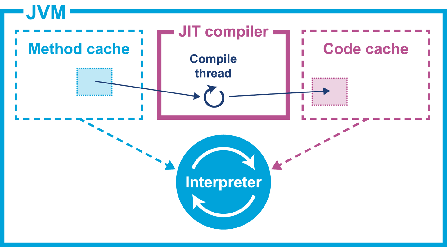
Figure 9-6. Simple compilation of a single method
When the optimized machine code is available, the entry in the vtable of the relevant klass is updated to point at the new compiled code.
This means that any new calls to the method will get the compiled form, whereas threads that are currently executing the interpreted form will finish the current invocation in interpreted mode, but will pick up the new compiled form on the next call.
OpenJDK has been widely ported to many different architectures with x86, x86-64, and ARM being the primary targets. SPARC, Power, MIPS, and S390 are also supported to varying degrees. Oracle officially supports Linux, macOS, and Windows as operating systems. There are open source projects to natively support a much wider selection, including BSDs and embedded systems.
Logging JIT Compilation
One important JVM switch that all performance engineers should know about is:
-XX:+PrintCompilation
This will cause a log of compilation events to be produced on STDOUT and will allow the engineer to get a basic understanding of what is being compiled.
For example, if the caching example from Example 3-1 is invoked like this:
java -XX:+PrintCompilation optjava.Caching 2>/dev/null
Then the resulting log (under Java 8) will look something like this:
56   1      3  java.lang.Object::<init> (1 bytes)
57   2      3  java.lang.String::hashCode (55 bytes)
58   3      3  java.lang.Math::min (11 bytes)
59   4      3  java.lang.String::charAt (29 bytes)
60   5      3  java.lang.String::length (6 bytes)
60   6      3  java.lang.String::indexOf (70 bytes)
60   7      3  java.lang.AbstractStringBuilder::ensureCapacityInternal (27 bytes)
60   8    n 0  java.lang.System::arraycopy (native)   (static)
60   9      1  java.lang.Object::<init> (1 bytes)
60   1      3  java.lang.Object::<init> (1 bytes)   made not entrant
61  10      3  java.lang.String::equals (81 bytes)
66  11      3  java.lang.AbstractStringBuilder::append (50 bytes)
67  12      3  java.lang.String::getChars (62 bytes)
68  13      3  java.lang.String::<init> (82 bytes)
74  14 %    3  optjava.Caching::touchEveryLine @ 2 (28 bytes)
74  15      3  optjava.Caching::touchEveryLine (28 bytes)
75  16 %    4  optjava.Caching::touchEveryLine @ 2 (28 bytes)
76  17 %    3  optjava.Caching::touchEveryItem @ 2 (28 bytes)
76  14 %    3  optjava.Caching::touchEveryLine @ -2 (28 bytes)   made not entrant
Note that as the vast majority of the JRE standard libraries are written in Java, they will be eligible for JIT compilation alongside application code. We should therefore not be surprised to see so many non-application methods present in the compiled code.
Tip
The exact set of methods that are compiled may vary slightly from run to run, even on a very simple benchmark. This is a side effect of the dynamic nature of PGO and should not be of concern.
The PrintCompilation output is formatted in a relatively simple way.
First comes the time at which a method was compiled (in ms since VM start).
Next is a number that indicates the order in which the method was compiled in this run. Some of the other fields are:
-
n: Method is native -
s: Method is synchronized -
!: Method has exception handlers -
%: Method was compiled via on-stack replacement
The level of detail available from PrintCompilation is somewhat limited.
To access more detailed information about the decisions made by the HotSpot JIT compilers, we can use:
-XX:+LogCompilation
This is a diagnostic option we must unlock using an additional flag:
-XX:+UnlockDiagnosticVMOptions
This instructs the VM to output a logfile containing XML tags representing information about the queuing and optimization of bytecode into native code.
The LogCompilation flag can be verbose and generate hundreds of MB of XML output.
However, as we will see in the next chapter, the open source JITWatch tool can parse this file and present the information in a more easily digestible format.
Other VMs, such as IBM’s J9 with the Testarossa JIT, can also be made to log JIT compiler information, but there is no standard format for JIT logging so developers must learn to interpret each log format or use appropriate tooling.
Compilers Within HotSpot
The HotSpot JVM actually has not one, but two JIT compilers in it. These are properly known as C1 and C2, but are sometimes referred to as the client compiler and the server compiler, respectively. Historically, C1 was used for GUI apps and other “client” programs, whereas C2 was used for long-running “server” applications. Modern Java apps generally blur this distinction, and HotSpot has changed to take advantage of the new landscape.
Note
A compiled code unit is known as an nmethod (short for native method).
The general approach that both compilers take is to rely on a key measurement to trigger compilation: the number of times a method is invoked, or the invocation count. Once this counter hits a certain threshold the VM is notified and will consider queuing the method for compilation.
The compilation process proceeds by first creating an internal representation of the method. Next, optimizations are applied that take into account profiling information that has been collected during the interpreted phase. However, the internal representation of the code that C1 and C2 produce is quite different. C1 is designed to be simpler and have shorter compile times than C2. The tradeoff is that as a result C1 does not optimize as fully as C2.
One technique that is common to both is single static assignment.
This essentially converts the program to a form where no reassignment of variables occurs.
In Java programming terms, the program is effectively rewritten to contain only final variables.
Tiered Compilation in HotSpot
Since Java 6, the JVM has supported a mode called tiered compilation. This is often loosely explained as running in interpreted mode until the simple C1 compiled form is available, then switching to using that compiled code while C2 completes more advanced optimizations.
However, this description is not completely accurate. From the advancedThresholdPolicy.hpp source file, we can see that within the VM there are five possible levels of execution:
-
Level 0: interpreter
-
Level 1: C1 with full optimization (no profiling)
-
Level 2: C1 with invocation and backedge counters
-
Level 3: C1 with full profiling
-
Level 4: C2
We can also see in Table 9-6 that not every level is utilized by each compilation approach.
| Pathway | Description |
|---|---|
0-3-4 |
Interpreter, C1 with full profiling, C2 |
0-2-3-4 |
Interpreter, C2 busy so quick-compile C1, then full-compile C1, then C2 |
0-3-1 |
Trivial method |
0-4 |
No tiered compilation (straight to C2) |
In the case of the trivial method, the method starts off interpreted as usual but then C1 (with full profiling) is able to determine the method to be trivial. This means that it is clear that the C2 compiler would produce no better code than C2 and so compilation terminates.
Tiered compilation has been the default for some time now, and it is not normally necessary to adjust its operation during performance tuning. An awareness of its operation is useful, though, as it can frequently complicate the observed behavior of compiled methods and potentially mislead the unwary engineer.
The Code Cache
JIT-compiled code is stored in a memory region called the code cache. This area also stores other native code belonging to the VM itself, such as parts of the interpreter.
The code cache has a fixed maximum size that is set at VM startup. It cannot expand past this limit, so it is possible for it to fill up. At this point no further JIT compilations are possible and uncompiled code will execute only in the interpreter. This will have an impact on performance and may result in the application being significantly less performant than the potential maximum.
The code cache is implemented as a heap containing an unallocated region and a linked list of freed blocks. Each time native code is removed, its block is added to the free list. A process called the sweeper is responsible for recycling blocks.
When a new native method is to be stored, the free list is searched for a block large enough to store the compiled code. If none is found, then subject to the code cache having sufficient free space, a new block will be created from the unallocated space.
Native code can be removed from the code cache when:
-
It is deoptimized (an assumption underpinning a speculative optimization turned out to be false).
-
It is replaced with another compiled version (in the case of tiered compilation).
-
The class containing the method is unloaded.
You can control the maximum size of the code cache using the VM switch:
-XX:ReservedCodeCacheSize=<n>
Note that with tiered compilation enabled, more methods will reach the lower compilation thresholds of the C1 client compiler. To account for this, the default maximum size is larger to hold these additional compiled methods.
In Java 8 on Linux x86-64 the default maximum sizes for the code cache are:
251658240 (240MB) when tiered compilation is enabled (-XX:+TieredCompilation)
 50331648  (48MB) when tiered compilation is disabled (-XX:-TieredCompilation)
Fragmentation
In Java 8 and earlier, the code cache can become fragmented if many of the intermediate compilations from the C1 compiler are removed after they are replaced by C2 compilations. This can lead to the unallocated region being used up and all of the free space residing in the free list.
The code cache allocator will have to traverse the linked list until it finds a block big enough to hold the native code of a new compilation. In turn, the sweeper will also have to more work to do scanning for blocks that can be recycled to the free list.
In the end, any garbage collection scheme that does not relocate memory blocks will be subject to fragmentation, and the code cache is not an exception.
Without a compaction scheme, the code cache can fragment and this can cause compilation to stop—it is just another form of cache exhaustion, after all.
Simple JIT Tuning
When undertaking a code tuning exercise, it is relatively easy to ensure that the application is taking advantage of JIT compilation.
The general principle of simple JIT compilation tuning is simple: “any method that wants to compile should be given the resources to do so.” To achieve this aim, follow this simple checklist:
-
First run the app with the
PrintCompilationswitch on. -
Collect the logs that indicate which methods are compiled.
-
Now increase the size of the code cache via
ReservedCodeCacheSize. -
Rerun the application.
-
Look at the set of compiled methods with the enlarged cache.
The performance engineer will need to take into account the slight nondeterminism inherent in the JIT compilation. Keeping this in mind, there are a couple of obvious tells that can easily be observed:
-
Is the set of compiled methods larger in a meaningful way when the cache size is increased?
-
Are all methods that are important to the primary transaction paths being compiled?
If the number of compiled methods does not increase (indicating that the code cache is not being fully utilized) as the cache size is increased, then provided the load pattern is representative, the JIT compiler is not short of resources.
At this point, it should be straightforward to confirm that all the methods that are part of the transaction hot paths appear in the compilation logs. If not, then the next step is to determine the root cause—why these methods are not compiling.
Effectively, this strategy is making sure that JIT compilation never shuts off, by ensuring that the JVM never runs out of code cache space.
We will meet more sophisticated techniques later in the book, but despite minor variations between Java versions, the simple JIT tuning approach can help provide performance boosts for a surprising number of applications.
Summary
The JVM’s initial code execution environment is the bytecode interpreter. We have explored the basics of the interpreter, as a working knowledge of bytecode is essential for a proper understanding of JVM code execution. The basic theory of JIT compilation has also been introduced.
However, for most performance work, the behavior of JIT-compiled code is far more important than any aspect of the interpreter. In the next chapter, we will build on the primer introduced here and dive deep into the theory and practice of JIT compilation.
For many applications the simple tuning of the code cache shown in this chapter will be sufficient. Applications that are particularly performance-sensitive may require a deeper exploration of JIT behavior. The next chapter will also describe tools and techniques to tune applications that have these more stringent requirements.