Table of Contents for
Optimizing Java
 Optimizing Java
Published by
O'Reilly Media, Inc., 2018
Optimizing Java
Published by
O'Reilly Media, Inc., 2018
- nav
- Cover
- Optimizing Java
- Optimizing Java
- Dedication
- Foreword
- Preface
- 1. Optimization and Performance Defined
- 2. Overview of the JVM
- 3. Hardware and Operating Systems
- 4. Performance Testing Patterns and Antipatterns
- 5. Microbenchmarking and Statistics
- 6. Understanding Garbage Collection
- 7. Advanced Garbage Collection
- 8. GC Logging, Monitoring, Tuning, and Tools
- 9. Code Execution on the JVM
- 10. Understanding JIT Compilation
- 11. Java Language Performance Techniques
- 12. Concurrent Performance Techniques
- 13. Profiling
- 14. High-Performance Logging and Messaging
- 15. Java 9 and the Future
- Index
- About the Authors
- Colophon
Chapter 8. GC Logging, Monitoring, Tuning, and Tools
In this chapter, we will introduce the huge subject of GC logging and monitoring. This is one of the most important and visible aspects of Java performance tuning, and also one of the most often misunderstood.
Introduction to GC Logging
The GC log is a great source of information. It is especially useful for “cold case” analysis of performance problems, such as providing some insight into why a crash occurred. It can allow the analyst to work, even with no live application process to diagnose.
Every serious application should always:
-
Generate a GC log.
-
Keep it in a separate file from application output.
This is especially true for production applications. As we’ll see, GC logging has no real observable overhead, so it should always be on for any important JVM process.
Switching On GC Logging
The first thing to do is to add some switches to the application startup. These are best thought of as the “mandatory GC logging flags,” which should be on for any Java/JVM application (except, perhaps, desktop apps). The flags are:
-Xloggc:gc.log -XX:+PrintGCDetails -XX:+PrintTenuringDistribution
-XX:+PrintGCTimeStamps -XX:+PrintGCDateStamps
Let’s look at each of these flags in more detail. Their usage is described in Table 8-1.
| Flag | Effect |
|---|---|
|
Controls which file to log GC events to |
|
Logs GC event details |
|
Adds extra GC event detail that is vital for tooling |
|
Prints the time (in secs since VM start) at which GC events occurred |
|
Prints the wallclock time at which GC events occurred |
The performance engineer should take note of the following details about some of these flags:
-
The
PrintGCDetailsflag replaces the olderverbose:gc. Applications should remove the older flag. -
The
PrintTenuringDistributionflag is different from the others, as the information it provides is not easily usable directly by humans. The flag provides the raw data needed to compute key memory pressure effects and events such as premature promotion. -
Both
PrintGCDateStampsandPrintGCTimeStampsare required, as the former is used to correlate GC events to application events (in application logfiles) and the latter is used to correlate GC and other internal JVM events.
This level of logging detail will not have a measurable effect on the JVM’s performance. The amount of logs generated will, of course, depend on many factors, including the allocation rate, the collector in use, and the heap size (smaller heaps will need to GC more frequently and so will produce logs more quickly).
To give you some idea, a 30-minute run of the model allocator example (as seen in Chapter 6) produces ~600 KB of logs for a 30-minute run, allocating 50 MB per second.
In addition to the mandatory flags, there are also some flags (shown in Table 8-2) that control GC log rotation, which many application support teams find useful in production environments.
| Flag | Effect |
|---|---|
|
Switches on logfile rotation |
|
Sets the maximum number of logfiles to keep |
|
Sets the maximum size of each file before rotation |
The setup of a sensible log rotation strategy should be done in conjunction with operations staff (including devops). Options for such a strategy, and a discussion of appropriate logging and tools, is outside the scope of this book.
GC Logs Versus JMX
In “Monitoring and Tooling for the JVM” we met the VisualGC tool, which is capable of displaying a real-time view of the state of the JVM’s heap. This tool actually relies on the Java Management eXtensions (JMX) interface to collect the data from the JVM. A full discussion of JMX is outside the scope of this book, but as far as JMX impacts GC, the performance engineer should be aware of the following:
-
GC log data is driven by actual garbage collection events, whereas JMX sourced data is obtained by sampling.
-
GC log data is extremely low-impact to capture, whereas JMX has implicit proxying and Remote Method Invocation (RMI) costs.
-
GC log data contains over 50 aspects of performance data relating to Java’s memory management, whereas JMX has less than 10.
Traditionally, one advantage that JMX has had over logs as a performance data source is that JMX can provide streamed data out of the box. However, modern tools such as jClarity Censum (see “Log Parsing Tools”) provide APIs to stream GC log data, closing this gap.
Warning
For a rough trend analysis of basic heap usage, JMX is a fairly quick and easy solution; however, for deeper diagnosis of problems it quickly becomes underpowered.
The beans made available via JMX are a standard and are readily accessible. The VisualVM tool provides one way of visualizing the data, and there are plenty of other tools available in the market.
Drawbacks of JMX
Clients monitoring an application using JMX will usually rely on sampling the runtime to get an update on the current state. To get a continuous feed of data, the client needs to poll the JMX beans in that runtime.
In the case of garbage collection, this causes a problem: the client has no way of knowing when the collector ran. This also means that the state of memory before and after each collection cycle is unknown. This rules out performing a range of deeper and more accurate analysis techniques on the GC data.
Analysis based on data from JMX is still useful, but it is limited to determining long-term trends. However, if we want to accurately tune a garbage collector we need to do better. In particular, being able to understand the state of the heap before and after each collection is extremely useful.
Additionally there is a set of extremely important analyses around memory pressure (i.e., allocation rates) that are simply not possible due to the way data is gathered from JMX.
Not only that, but the current implementation of the JMXConnector specification relies on RMI. Thus, use of JMX is subject to the same issues that arise with any RMI-based communication channel. These include:
-
Opening ports in firewalls so secondary socket connections can be established
-
Using proxy objects to facilitate
remove()method calls -
Dependency on Java finalization
For a few RMI connections, the amount of work involved to close down a connection is minuscule. However, the teardown relies upon finalization. This means that the garbage collector has to run to reclaim the object.
The nature of the lifecycle of the JMX connection means that most often this will result in the RMI object not being collected until a full GC. See “Avoid Finalization” for more details about the impact of finalization and why it should always be avoided.
By default, any application using RMI will cause full GCs to be triggered once an hour. For applications that are already using RMI, using JMX will not add to the costs. However, applications not already using RMI will necessarily take an additional hit if they decide to use JMX.
Benefits of GC Log Data
Modern-day garbage collectors contain many different moving parts that, put together, result in an extremely complex implementation. So complex is the implementation that the performance of a collector is seemingly difficult if not impossible to predict. These types of software systems are known as emergent, in that their final behavior and performance is a consequence of how all of the components work and perform together. Different pressures stress different components in different ways, resulting in a very fluid cost model.
Initially Java’s GC developers added GC logging to help debug their implementations, and consequently a significant portion of the data produced by the almost 60 GC-related flags is for performance debugging purposes.
Over time those tasked with tuning the garbage collection process in their applications came to recognize that given the complexities of tuning GC, they also benefitted from having an exact picture of what was happening in the runtime. Thus, being able to collect and read GC logs is now an instrumental part of any tuning regime.
Tip
GC logging is done from within the HotSpot JVM using a nonblocking writing mechanism. It has ~0% impact on application performance and should be switched on for all production applications.
Because the raw data in the GC logs can be pinned to specific GC events, we can perform all kinds of useful analyses on it that can give us insights into the costs of the collection, and consequently which tuning actions are more likely to produce positive results.
Log Parsing Tools
There is no language or VM spec standard format for GC log messages. This leaves the content of any individual message to the whim of the HotSpot GC development team. Formats can and do change from minor release to minor release.
This is further complicated by the fact that, while the simplest log formats are easy to parse, as GC log flags are added the resulting log output becomes massively more complicated. This is especially true of the logs generated by the concurrent collectors.
All too often, systems with hand-rolled GC log parsers experience an outage at some point after changes are made to the GC configuration, that alter the log output format. When the outage investigation turns to examining the GC logs, the team finds that the homebrew parser cannot cope with the changed log format—failing at the exact point when the log information is most valuable.
Warning
It is not recommended that developers attempt to parse GC logs themselves. Instead, a tool should be used.
In this section, we will examine two actively maintained tools (one commercial and one open source) that are available for this purpose. There are others, such as GarbageCat, that are maintained only sporadically, or not at all.
Censum
The Censum memory analyzer is a commercial tool developed by jClarity. It is available both as a desktop tool (for hands-on analysis of a single JVM) and as a monitoring service (for large groups of JVMs). The aim of the tool is to provide best-available GC log parsing, information extraction, and automated analytics.
In Figure 8-1, we can see the Censum desktop view showing allocation rates for a financial trading application running the G1 garbage collector. Even from this simple view we can see that the trading application has periods of very low allocation, corresponding to quiet periods in the market.
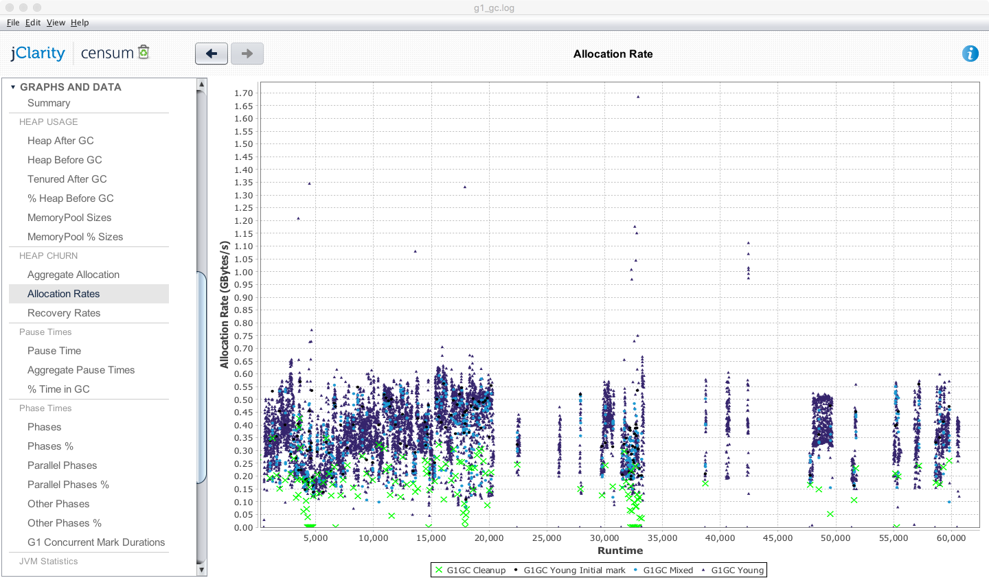
Figure 8-1. Censum allocation view
Other views available from Censum include the pause time graph, shown in Figure 8-2 from the SaaS version.
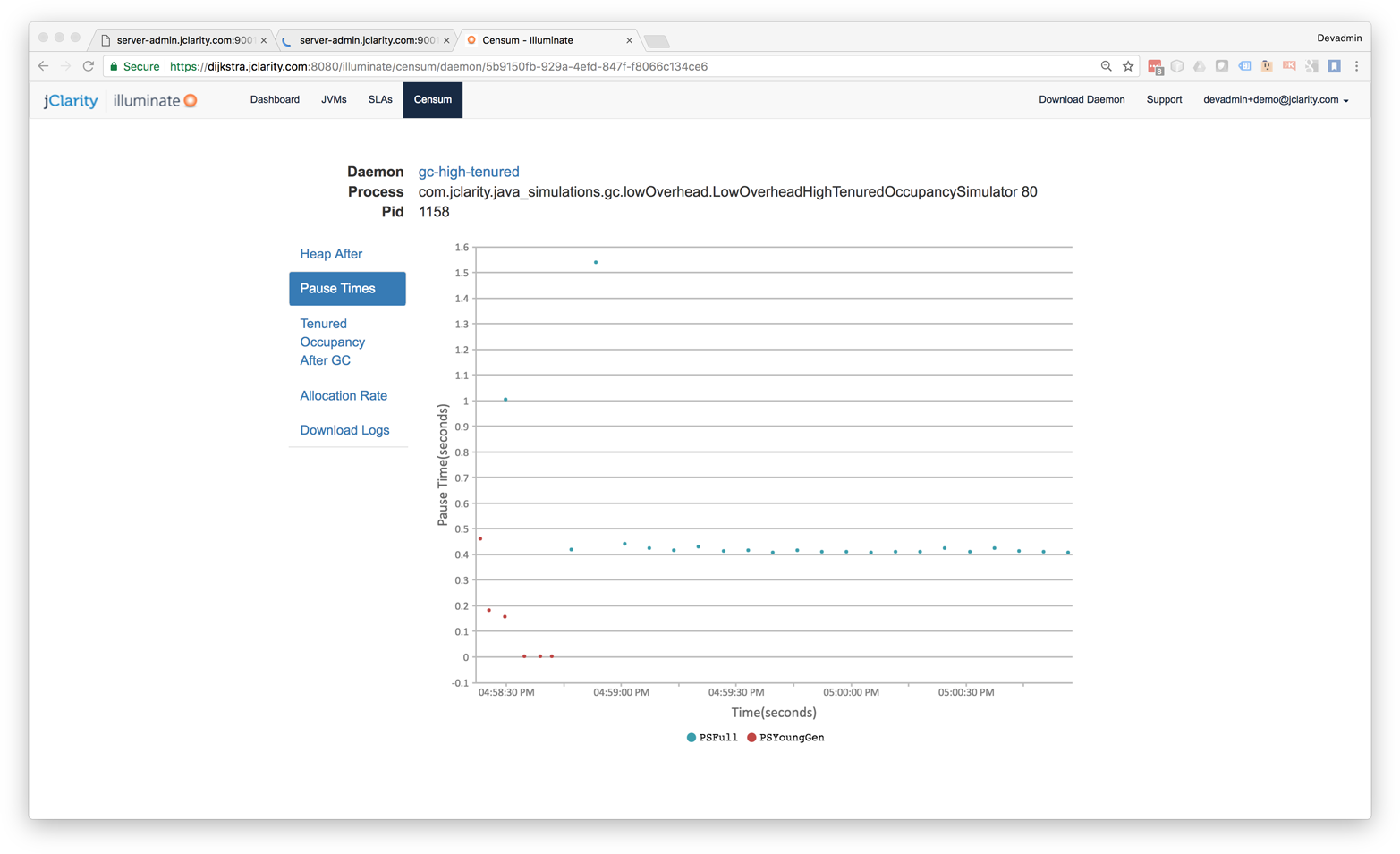
Figure 8-2. Censum pause time view
One of the advantages of using the Censum SAAS monitoring service is being able to view the health of an entire cluster simultaneously, as in Figure 8-3. For ongoing monitoring, this is usually easier than dealing with a single JVM at a time.
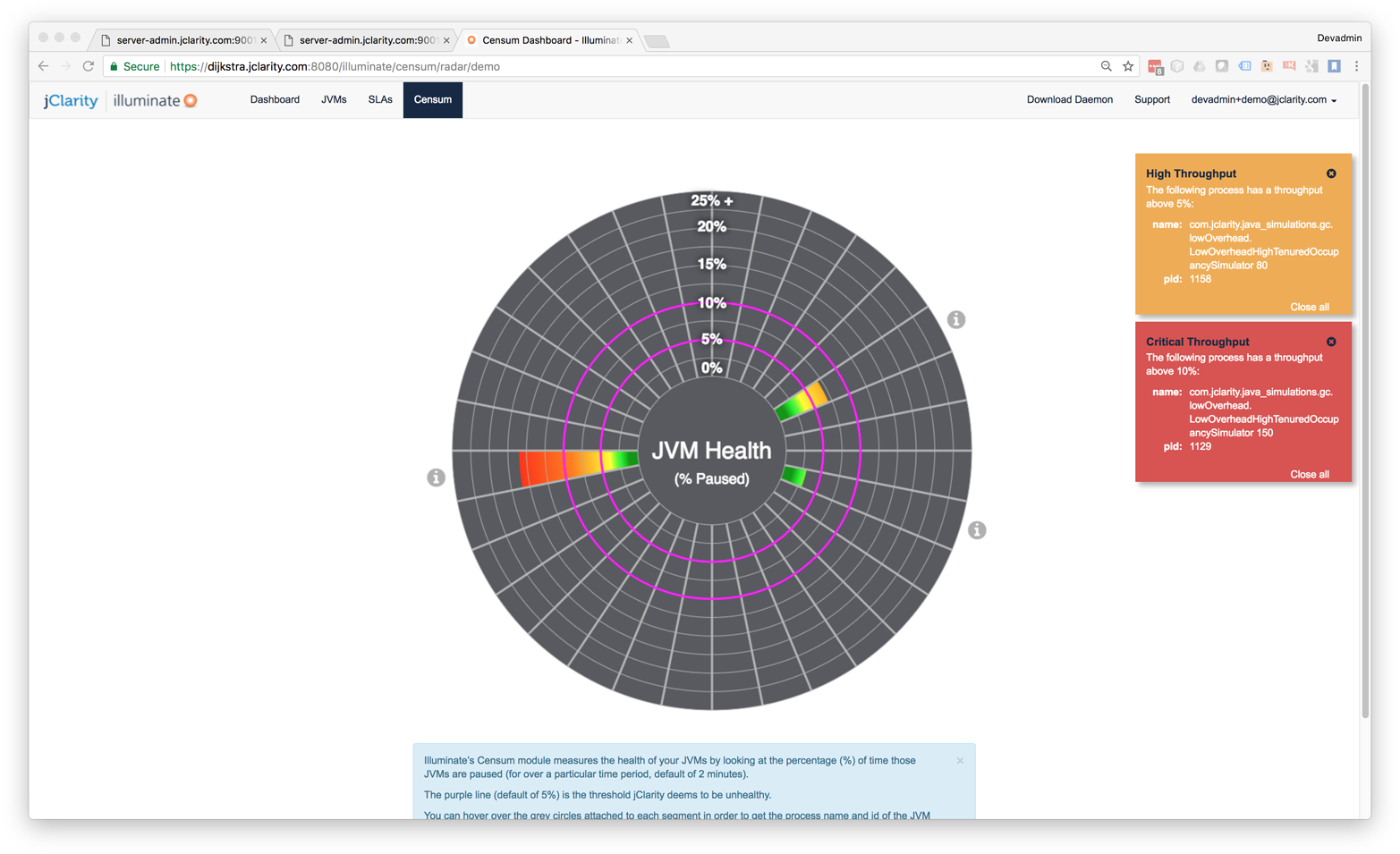
Figure 8-3. Censum cluster health overview
Censum has been developed with close attention to the logfile formats, and all checkins to OpenJDK that could affect logging are monitored. Censum supports all versions of Sun/Oracle Java from 1.4.2 to current, all collectors, and the largest number of GC log configurations of any tool in the market.
As of the current version, Censum supports these automatic analytics:
-
Accurate allocation rates
-
Premature promotion
-
Aggressive or “spiky” allocation
-
Idle churn
-
Memory leak detection
-
Heap sizing and capacity planning
-
OS interference with the VM
-
Poorly sized memory pools
More details about Censum, and trial licenses, are available from the jClarity website.
GCViewer
GCViewer is a desktop tool that provides some basic GC log parsing and graphing capabilities. Its big positives are that it is open source software and is free to use. However, it does not have many features as compared to the commercial tools.
To use it, you will need to download the source. After compiling and building it, you can package into an executable JAR file.
GC logfiles can then be opened in the main GCViewer UI. An example is shown in Figure 8-4.
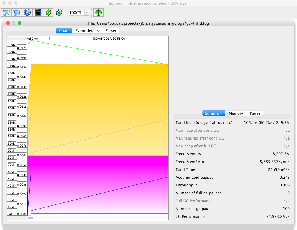
Figure 8-4. GCViewer
GCViewer lacks analytics and can parse only some of the possible GC log formats that HotSpot can produce.
It is possible to use GCViewer as a parsing library and export the data points into a visualizer, but this requires additional development on top of the existing open source code base.
Different Visualizations of the Same Data
You should be aware that different tools may produce different visualizations of the same data. The simple sawtooth pattern that we met in “The Role of Allocation” was based on a sampled view of the overall size of the heap as the observable.
When the GC log that produced this pattern is plotted with the “Heap Occupancy after GC” view of GCViewer, we end up with the visualization shown in Figure 8-5.
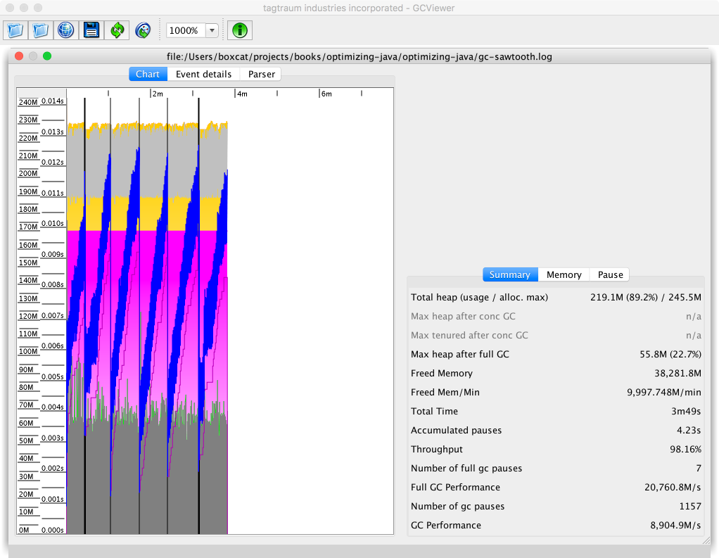
Figure 8-5. Simple sawtooth in GCViewer
Let’s look at the same simple sawtooth pattern displayed in Censum. Figure 8-6 shows the result.
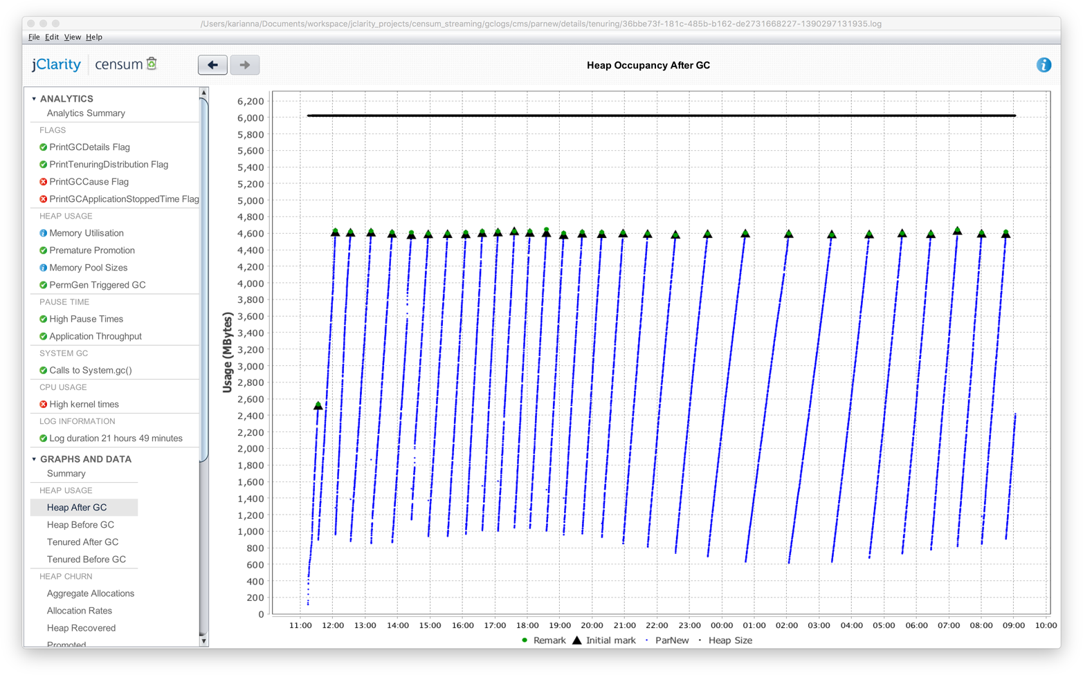
Figure 8-6. Simple sawtooth in Censum
While the images and visualizations are different, the message from the tool is the same in both cases—that the heap is operating normally.
Basic GC Tuning
When engineers are considering strategies for tuning the JVM, the question “When should I tune GC?” often arises. As with any other tuning technique, GC tuning should form part of an overall diagnostic process. The following facts about GC tuning are very useful to remember:
-
It’s cheap to eliminate or confirm GC as the cause of a performance problem.
-
It’s cheap to switch on GC flags in UAT.
-
It’s not cheap to set up memory or execution profilers.
The engineer should also know that these four main factors should be studied and measured during a tuning exercise:
-
Allocation
-
Pause sensitivity
-
Throughput behavior
-
Object lifetime
Of these, allocation is very often the most important.
Note
Throughput can be affected by a number of factors, such as the fact that concurrent collectors take up cores when they’re running.
Let’s take a look at some of the basic heap sizing flags, listed in Table 8-3.
| Flag | Effect |
|---|---|
|
Sets the minimum size reserved for the heap |
|
Sets the maximum size reserved for the heap |
|
Sets the maximum size permitted for PermGen (Java 7) |
|
Sets the maximum size permitted for Metaspace (Java 8) |
The MaxPermSize flag is legacy and applies only to Java 7 and before. In Java 8 and up, the PermGen has been removed and replaced by Metaspace.
Note
If you are setting MaxPermSize on a Java 8 application, then you should just remove the flag. It is being ignored by the JVM anyway, so it clearly is having no impact on your application.
On the subject of additional GC flags for tuning:
-
Only add flags one at a time.
-
Make sure that you fully understand the effect of each flag.
-
Recall that some combinations produce side effects.
Checking whether GC is the cause of a performance issue is relatively easy, assuming the event is happening live.
The first step is to look at the machine’s high-level metrics using vmstat or a similar tool, as discussed in “Basic Detection Strategies”. First, log on to the box having the performance issue and check that:
-
CPU utilization is close to 100%.
-
The vast majority of this time (90+%) is being spent in user space.
-
The GC log is showing activity, indicating that GC is currently running.
This assumes that the issue is happening right now and can be observed by the engineer in real time. For past events, sufficient historical monitoring data must be available (including CPU utilization and GC logs that have timestamps).
If all three of these conditions are met, GC should be investigated and tuned as the most likely cause of the current performance issue. The test is very simple, and has a nice clear result—either that “GC is OK” or “GC is not OK.”
If GC is indicated as a source of performance problems, then the next step is to understand the allocation and pause time behavior, then tune the GC and potentially bring out the memory profiler if required.
Understanding Allocation
Allocation rate analysis is extremely important for determining not just how to tune the garbage collector, but whether or not you can actually tune the garbage collector to help improve performance at all.
We can use the data from the young generational collection events to calculate the amount of data allocated and the time between the two collections. This information can then be used to calculate the average allocation rate during that time interval.
Note
Rather than spending time and effort manually calculating allocation rates, it is usually better to use tooling to provide this number.
Experience shows that sustained allocation rates of greater than 1 GB/s are almost always indicative of performance problems that cannot be corrected by tuning the garbage collector. The only way to improve performance in these cases is to improve the memory efficiency of the application by refactoring to eliminate allocation in critical parts of the application.
A simple memory histogram, such as that shown by VisualVM (as seen in “Monitoring and Tooling for the JVM”) or even jmap (“Introducing Mark and Sweep”), can serve as a starting point for understanding memory allocation behavior.
A useful initial allocation strategy is to concentrate on four simple areas:
-
Trivial, avoidable object allocation (e.g., log debug messages)
-
Boxing costs
-
Domain objects
-
Large numbers of non-JDK framework objects
For the first of these, it is simply a matter of spotting and removing unnecessary object creation. Excessive boxing can be a form of this, but other examples (such as autogenerated code for serializing/deserializing to JSON, or ORM code) are also possible sources of wasteful object creation.
It is unusual for domain objects to be a major contributor to the memory utilization of an application. Far more common are types such as:
-
char[]: The characters that comprise strings -
byte[]: Raw binary data -
double[]: Calculation data -
Map entries
-
Object[] -
Internal data structures (such as methodOops and klassOops)
A simple histogram can often reveal leaking or excessive creation of unnecessary domain objects, simply by their presence among the top elements of a heap histogram. Often, all that is necessary is a quick calculation to figure out the expected data volume of domain objects, to see whether the observed volume is in line with expectations or not.
In “Thread-Local Allocation” we met thread-local allocation. The aim of this technique is to provide a private area for each thread to allocate new objects, and thus achieve O(1) allocation.
The TLABs are sized dynamically on a per-thread basis, and regular objects are allocated in the TLAB, if there’s space. If not, the thread requests a new TLAB from the VM and tries again.
If the object will not fit in an empty TLAB, the VM will next try to allocate the object directly in Eden, in an area outside of any TLAB. If this fails, the next step is to perform a young GC (which might resize the heap). Finally, if this fails and there’s still not enough space, the last resort is to allocate the object directly in Tenured.
From this we can see that the only objects that are really likely to end up being directly allocated in Tenured are large arrays (especially byte and char arrays).
HotSpot has a couple of tuning flags that are relevant to the TLABs and the pretenuring of large objects:
-XX:PretenureSizeThreshold=<n>
-XX:MinTLABSize=<n>
As with all switches, these should not be used without a benchmark and solid evidence that they will have an effect. In most cases, the built-in dynamic behavior will produce great results, and any changes will have little to no real observable impact.
Allocation rates also affect the number of objects that are promoted to Tenured. If we assume that short-lived Java objects have a fixed lifetime (when expressed in wallclock time), then higher allocation rates will result in young GCs that are closer together. If the collections become too frequent, then short-lived objects may not have had time to die and will be erroneously promoted to Tenured.
To put it another way, spikes in allocation can lead to the premature promotion problem that we met in “The Role of Allocation”. To guard against this, the JVM will resize survivor spaces dynamically to accommodate greater amounts of surviving data without promoting it to Tenured.
One JVM switch that can sometimes be helpful for dealing with tenuring problems and premature promotion is:
-XX:MaxTenuringThreshold=<n>
This controls the number of garbage collections that an object must survive to be promoted into Tenured. It defaults to 4 but can be set anywhere from 1 to 15. Changing this value represents a tradeoff between two concerns:
-
The higher the threshold, the more copying of genuinely long-lived objects will occur.
-
If the threshold is too low, some short-lived objects will be promoted, increasing memory pressure on Tenured.
One consequence of too low a threshold could be that full collections occur more often, due to the greater volume of objects being promoted to Tenured, causing it to fill up more quickly. As always, you should not alter the switch without a clear benchmark indicating that you will improve performance by setting it to a nondefault value.
Understanding Pause Time
Developers frequently suffer from cognitive bias about pause time. Many applications can easily tolerate 100+ ms pause times. The human eye can only process 5 updates per second of a single data item, so a 100–200 ms pause is below the threshold of visibility for most human-facing applications (such as web apps).
One useful heuristic for pause-time tuning is to divide applications into three broad bands. These bands are based on the application’s need for responsiveness, expressed as the pause time that the application can tolerate. They are:
-
>1 s: Can tolerate over 1 s of pause
-
1 s–100 ms: Can tolerate more than 200 ms but less than 1 s of pause
-
< 100 ms: Cannot tolerate 100 ms of pause
If we combine the pause sensitivity with the expected heap size of the application, we can construct a simple table of best guesses at a suitable collector. The result is shown in Table 8-4.
| Pause time tolerance | |||
|---|---|---|---|
>1 s |
1 s–100 ms |
<100 ms |
< 2 GB |
Parallel |
Parallel |
CMS |
< 4 GB |
Parallel |
Parallel/G1 |
CMS |
< 4 GB |
Parallel |
Parallel/G1 |
CMS |
< 10 GB |
Parallel/G1 |
Parallel/G1 |
CMS |
< 20 GB |
Parallel/G1 |
G1 |
CMS |
> 20 GB |
These are guidelines and rules of thumb intended as a starting point for tuning, not 100% unambiguous rules.
Looking into the future, as G1 matures as a collector, it is reasonable to expect that it will expand to cover more of the use cases currently covered by ParallelOld. It is also possible, but perhaps less likely, that it will expand to CMS’s use cases as well.
Tip
When a concurrent collector is in use, you should still reduce allocation before attempting to tune pause time. Reduced allocation means that there is less memory pressure on a concurrent collector; the collection cycles will find it easier to keep up with the allocating threads. This will reduce the possibility of a concurrent mode failure, which is usually an event that pause-sensitive applications need to avoid if at all possible.
Collector Threads and GC Roots
One useful mental exercise is to “think like a GC thread.” This can provide insight into how the collector behaves under various circumstances. However, as with so many other aspects of GC, there are fundamental tradeoffs in play. These tradeoffs include that the scanning time needed to locate GC roots is affected by factors such as:
-
Number of application threads
-
Amount of compiled code in the code cache
-
Size of heap
Even for this single aspect of GC, which one of these events dominates the GC root scanning will always depend on runtime conditions and the amount of parallelization that can be applied.
For example, consider the case of a large Object[] discovered in the Mark phase. This will be scanned by a single thread; no work stealing is possible. In the extreme case, this single-threaded scanning time will dominate the overall mark time.
In fact, the more complex the object graph, the more pronounced this effect becomes—meaning that marking time will get even worse the more “long chains” of objects exist within the graph.
High numbers of application threads will also have an impact on GC times, as they represent more stack frames to scan and more time needed to reach a safepoint. They also exert more pressure on thread schedulers in both bare metal and virtualized environments.
As well as these traditional examples of GC roots, there are also other sources of GC roots, including JNI frames and the code cache for JIT-compiled code (which we will meet properly in “The Code Cache”).
Warning
GC root scanning in the code cache is single-threaded (at least for Java 8).
Of the three factors, stack and heap scanning are reasonably well parallelized. Generational collectors also keep track of roots that originate in other memory pools, using mechanisms such as the RSets in G1 and the card tables in Parallel GC and CMS.
For example, let’s consider the card tables, introduced in “Weak Generational Hypothesis”. These are used to indicate a block of memory that has a reference back into young gen from old gen. As each byte represents 512 bytes of old gen, it’s clear that for each 1 GB of old gen memory, 2 MB of card table must be scanned.
To get a feel for how long a card table scan will take, consider a simple benchmark that simulates scanning a card table for a 20 GB heap:
@State(Scope.Benchmark)@BenchmarkMode(Mode.Throughput)@Warmup(iterations=5,time=1,timeUnit=TimeUnit.SECONDS)@Measurement(iterations=5,time=1,timeUnit=TimeUnit.SECONDS)@OutputTimeUnit(TimeUnit.SECONDS)@Fork(1)publicclassSimulateCardTable{// OldGen is 3/4 of heap, 2M of card table is required for 1G of old genprivatestaticfinalintSIZE_FOR_20_GIG_HEAP=15*2*1024*1024;privatestaticfinalbyte[]cards=newbyte[SIZE_FOR_20_GIG_HEAP];@Setuppublicstaticfinalvoidsetup(){finalRandomr=newRandom(System.nanoTime());for(inti=0;i<100_000;i++){cards[r.nextInt(SIZE_FOR_20_GIG_HEAP)]=1;}}@BenchmarkpublicintscanCardTable(){intfound=0;for(inti=0;i<SIZE_FOR_20_GIG_HEAP;i++){if(cards[i]>0)found++;}returnfound;}}
Running this benchmark results in an output similar to the following:
Result "scanCardTable":
  108.904 ±(99.9%) 16.147 ops/s [Average]
  (min, avg, max) = (102.915, 108.904, 114.266), stdev = 4.193
  CI (99.9%): [92.757, 125.051] (assumes normal distribution)


# Run complete. Total time: 00:01:46

Benchmark                         Mode  Cnt    Score    Error  Units
SimulateCardTable.scanCardTable  thrpt    5  108.904 ± 16.147  ops/s
This shows that it takes about 10 ms to scan the card table for a 20 GB heap. This is, of course, the result for a single-threaded scan; however, it does provide a useful rough lower bound for the pause time for young collections.
We’ve examined some general techniques that should be applicable to tuning most collectors, so now let’s move on to look at some collector-specific approaches.
Tuning Parallel GC
Parallel GC is the simplest of the collectors, and so it should be no surprise that it is also the easiest to tune. However, it usually requires minimal tuning. The goals and the tradeoffs of Parallel GC are clear:
-
Fully STW
-
High GC throughput/computationally cheap
-
No possibility of a partial collection
-
Linearly growing pause time in the size of the heap
If your application can tolerate the characteristics of Parallel GC, then it can be a very effective choice—especially on small heaps, such as those under ~4 GB.
Older applications may have made use of explicit sizing flags to control the relative size of various memory pools. These flags are summarized in Table 8-5.
| Flag | Effect |
|---|---|
|
(Old flag) Sets ratio of young gen to Heap |
|
(Old flag) Sets ratio of survivor spaces to young gen |
|
(Old flag) Sets min size of young gen |
|
(Old flag) Sets max size of young gen |
|
(Old flag) Sets min % of heap free after GC to avoid expanding |
|
(Old flag) Sets max % of heap free after GC to avoid shrinking |
The survivor ratio, new ratio, and overall heap size are connected by the following formula:
Flagsset:-XX:NewRatio=N-XX:SurvivorRatio=KYoungGen=1/(N+1)ofheapOldGen=N/(N+1)ofheapEden=(K–2)/KofYoungGenSurvivor1=1/KofYoungGenSurvivor2=1/KofYoungGen
For most modern applications, these types of explicit sizing should not be used, as the ergonomic sizing will do a better job than humans in almost all cases. For Parallel GC, resorting to these switches is something close to a last resort.
Tuning CMS
The CMS collector has a reputation of being difficult to tune. This is not wholly undeserved: the complexities and tradeoffs involved in getting the best performance out of CMS are not to be underestimated.
The simplistic position “pause time bad, therefore concurrent marking collector good” is unfortunately common among many developers. A low-pause collector like CMS should really be seen as a last resort, only to be used if the use case genuinely requires low STW pause times. To do otherwise may mean that a team is lumbered with a collector that is difficult to tune and provides no real tangible benefit to the application performance.
CMS has a very large number of flags (almost 100 as of Java 8u131), and some developers may be tempted to change the values of these flags in an attempt to improve performance. However, this can easily lead to several of the antipatterns that we met in Chapter 4, including:
-
Fiddling with Switches
-
Tuning by Folklore
-
Missing the Bigger Picture
The conscientious performance engineer should resist the temptation to fall prey to any of these cognitive traps.
Warning
The majority of applications that use CMS will probably not see any real observable improvement by changing the values of CMS command-line flags.
Despite this danger, there are some circumstances where tuning is necessary to improve (or obtain acceptable) CMS performance. Let’s start by considering the throughput behavior.
While a CMS collection is running, by default half the cores are doing GC. This inevitably causes application throughout to be reduced. One useful rule of thumb can be to consider the situation of the collector just before a concurrent mode failure occurs.
In this case, as soon as a CMS collection has finished, a new CMS collection immediately starts. This is known as a back-to-back collection, and in the case of a concurrent collector, it indicates the point at which concurrent collection is about to break down. If the application allocates any faster, then reclamation will be unable to keep up and the result will be a CMF.
In the back-to-back case, throughput will be reduced by 50% for essentially the entire run of the application. When undertaking a tuning exercise, the engineer should consider whether the application can tolerate this worst-case behavior. If not, then the solution may be to run on a host with more cores available.
An alternative is to reduce the number of cores assigned to GC during a CMS cycle. Of course, this is dangerous, as it reduces the amount of CPU time available to perform collection, and so will make the application less resilient to allocation spikes (and in turn may make it more vulnerable to a CMF). The switch that controls this is:
-XX:ConcGCThreads=<n>
It should be obvious that if an application cannot reclaim fast enough with the default setting, then reducing the number of GC threads will only make matters worse.
CMS has two separate STW phases:
- Initial Mark
-
Marks the immediate interior nodes—those that are directly pointed at by GC roots
- * Remark
-
Uses the card tables to identify objects that may require fixup work
This means that all app threads must stop, and hence safepoint, twice per CMS cycle. This effect can become important for some low-latency apps that are sensitive to safepointing behavior.
Two flags that are sometimes seen together are:
-XX:CMSInitiatingOccupancyFraction=<n>
-XX:+UseCMSInitiatingOccupancyOnly
These flags can be very useful. They also illustrate, once again, the importance of and dilemma presented by unstable allocation rates.
The initiating occupancy flag is used to determine at what point CMS should begin collecting. Some heap headroom is required so that there’s spare space for objects to be promoted into from young collections that may occur while CMS is running.
Like many other aspects of HotSpot’s approach to GC, the size of this spare space is controlled by the statistics collected by the JVM itself. However, an estimate for the first run of CMS is still required. The headroom size for this initial guess is controlled by the flag CMSInitiatingOccupancyFraction. The default for this flag means that the first CMS full GC will begin when the heap is 75% full.
If the UseCMSInitiatingOccupancyOnly flag is also set, then the dynamic sizing for the initiating occupancy is turned off. This should not be done lightly, and it is rare in practice to decrease the headroom (increase the parameter value above 75%).
However, for some CMS applications that have very bursty allocation rates, one strategy would be to increase the headroom (decrease the parameter value) while turning off the adaptive sizing. The aim here would be to try to reduce concurrent mode failures, at the expense of CMS concurrent GCs occurring more often.
Concurrent Mode Failures Due to Fragmentation
Let’s look at another case where the data we need to perform a tuning analysis is only available in the GC logs. In this case we want to use the free list statistics to predict when the JVM might suffer from a CMF due to heap fragmentation. This type of CMF is caused by the free list that CMS maintains, which we met in “JVM Safepoints”.
We will need to turn on another JVM switch to see the additional output:
-XX:PrintFLSStatistics=1
The output that’s produced in the GC log looks like this (detail of output statistics shown for a BinaryTreeDictionary benchmark):
Total Free Space: 40115394

Max Chunk Size: 38808526

Number of Blocks: 1360

Av. Block Size: 29496

Tree Height: 22
In this case we can get a sense of the size distribution of chunks of memory from the average size and the max chunk size. If we run out of chunks large enough to support moving a large live object into Tenured, then a GC promotion will degrade into this concurrent failure mode.
In order to compact the heap and coalesce the free space list, the JVM will fall back to Parallel GC, probably causing a long STW pause. This analysis is useful when performed in real time, as it can signal that a long pause is imminent. You can observe it by parsing the logs, or using a tool like Censum that can automatically detect the approaching CMF.
Tuning G1
The overall goal of tuning G1 is to allow the end user to simply set the maximum heap size and MaxGCPauseMillis, and have the collector take care of everything else. However, the current reality is still some way from this.
Like CMS, G1 comes with a large number of configuration options, some of which are still experimental and not fully surfaced within the VM (in terms of visible metrics for tuning). This makes it difficult to understand the impact of any tuning changes. If these options are needed for tuning (and currently they are for some tuning scenarios), then this switch must be specified:
-XX:+UnlockExperimentalVMOptions
In particular, this option must be specified if the options -XX:G1NewSizePercent=<n> or -XX:G1MaxNewSizePercent=<n> are to be used. At some point in the future, some of these options may become more mainstream and not require the experimental options flag, but there is no roadmap for this yet.
An interesting view of the G1 heap can be seen in Figure 8-7. This image was generated by the regions JavaFX application.
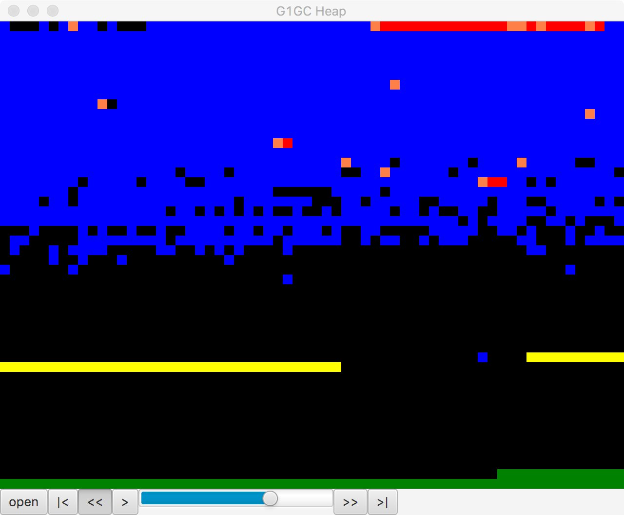
Figure 8-7. Visualizing G1’s heap in regions
This is a small, open source Java FX application that parses a G1 GC log and provides a way to visualize the region layout of a G1 heap over the lifetime of a GC log. The tool was written by Kirk Pepperdine and can be obtained from GitHub. At the time of writing it is still under active development.
One of the major issues with G1 tuning is that the internals have changed considerably over the early life of the collector. This has led to a significant problem with Tuning by Folklore, as many of the earlier articles that were written about G1 are now of limited validity.
With G1 becoming the default collector as of Java 9, performance engineers will surely be forced to address the topic of how to tune G1, but as of this writing it remains an often frustrating task where best practice is still emerging.
However, let’s finish this section by focusing on where some progress has been made, and where G1 does offer the promise of exceeding CMS. Recall that CMS does not compact, so over time the heap can fragment. This will lead to a concurrent mode failure eventually and the JVM will need to perform a full parallel collection (with the possibility of a significant STW pause).
In the case of G1, provided the collector can keep up with the allocation rate, then the incremental compaction offers the possibility of avoiding a CMF at all. An application that has a high, stable allocation rate and which creates mostly short-lived options should therefore:
-
Set a large young generation.
-
Increase the tenuring threshold, probably to the maximum (15).
-
Set the longest pause time goal that the app can tolerate.
Configuring Eden and survivor spaces in this way gives the best chance that genuinely short-lived objects are not promoted. This reduces pressure on the old generation and reduces the need to clean old regions. There are rarely any guarantees in GC tuning, but this is an example workload where G1 may do significantly better than CMS, albeit at the cost of some effort to tune the heap.
jHiccup
We already met HdrHistogram in “Non-Normal Statistics”. A related tool is jHiccup, available from GitHub. This is an instrumentation tool that is designed to show “hiccups” where the JVM is not able to run continuously. One very common cause of this is GC STW pauses, but other OS- and platform-related effects can also cause a hiccup. It is therefore useful not only for GC tuning but for ultra-low-latency work.
In fact, we have also already seen an example of how jHiccup works. In “Shenandoah” we introduced the Shenandoah collector, and showcased a graph of the collector’s performance as compared to others. The graph of comparative performance in Figure 7-9 was produced by JHiccup.
Note
jHiccup is an excellent tool to use when you are tuning HotSpot, even though the original author (Gil Tene) cheerfully admits that it was written to show up a perceived shortcoming of HotSpot as compared to Azul’s Zing JVM.
jHiccup is usually used as a Java agent, by way of the -javaagent:jHiccup.jar Java command-line switch. It can also be used via the Attach API (like some of the other command-line tools). The form for this is:
jHiccup -p <pid>
This effectively injects jHiccup into a running application.
jHiccup produces output in the form of a histogram log that can be ingested by HdrHistogram. Let’s take a look at this in action, starting by recalling the model allocation application introduced in “The Role of Allocation”.
To run this with a set of decent GC logging flags as well as jHiccup running as an agent, let’s look at a small piece of shell scripting to set up the run:
#!/bin/bash# Simple script for running jHiccup against a run of the model toy allocatorCP=./target/optimizing-java-1.0.0-SNAPSHOT.jarJHICCUP_OPTS=-javaagent:~/.m2/repository/org/jhiccup/jHiccup/2.0.7/jHiccup-2.0.7.jarGC_LOG_OPTS="-Xloggc:gc-jHiccup.log -XX:+PrintGCDetails -XX:+PrintGCDateStamps-XX:+PrintGCTimeStamps -XX:+PrintTenuringDistribution"MEM_OPTS="-Xmx1G"JAVA_BIN=`which java`if[$JAVA_HOME];thenJAVA_CMD=$JAVA_HOME/bin/javaelif[$JAVA_BIN];thenJAVA_CMD=$JAVA_BINelseecho"For this command to run, either$JAVA_HOMEmust be set, or java must bein the path."exit1fiexec$JAVA_CMD-cp$CP$JHICCUP_OPTS$GC_LOG_OPTS$MEM_OPTSoptjava.ModelAllocator
This will produce both a GC log and an .hlog file suitable to be fed to the jHiccupLogProcessor tool that ships as part of jHiccup. A simple, out-of-the-box jHiccup view is shown in Figure 8-8.
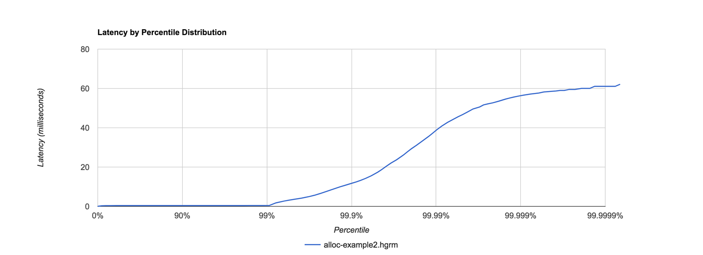
Figure 8-8. jHiccup view of ModelAllocator
This was obtained by a very simple invocation of jHiccup:
jHiccupLogProcessor -i hiccup-example2.hlog -o alloc-example2
There are some other useful switches—to see all the available options, just use:
jHiccupLogProcessor -h
It is very often the case that performance engineers need to comprehend multiple views of the same application behavior, so for completeness, let’s see the same run as seen from Censum, in Figure 8-9.
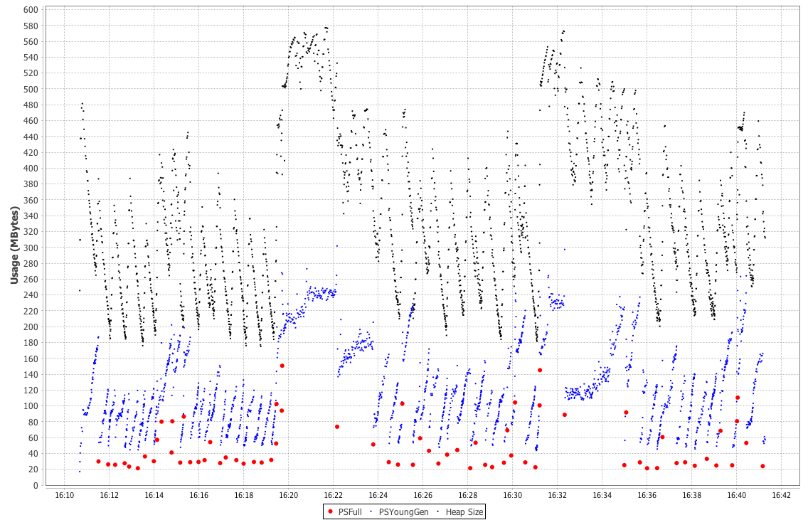
Figure 8-9. Censum view of ModelAllocator
This graph of the heap size after GC reclamation shows HotSpot trying to resize the heap and not being able to find a stable state. This is a frequent circumstance, even for applications as simple as ModelAllocator. The JVM is a very dynamic environment, and for the most part developers should avoid being overly concerned with the low-level detail of GC ergonomics.
Finally, some very interesting technical details about both HdrHistogram and jHiccup can be found in a great blog post by Nitsan Wakart.
Summary
In this chapter we have scratched the surface of the art of GC tuning. The techniques we have shown are mostly highly specific to individual collectors, but there are some underlying techniques that are generally applicable. We have also covered some basic principles for handling GC logs, and met some useful tools.
Moving onward, in the next chapter we will turn to one of the other major subsystems of the JVM: execution of application code. We will begin with an overview of the interpreter and then proceed from there to a discussion of JIT compilation, including how it relates to standard (or “Ahead-of-Time”) compilation.