Table of Contents for
Optimizing Java
 Optimizing Java
Published by
O'Reilly Media, Inc., 2018
Optimizing Java
Published by
O'Reilly Media, Inc., 2018
- nav
- Cover
- Optimizing Java
- Optimizing Java
- Dedication
- Foreword
- Preface
- 1. Optimization and Performance Defined
- 2. Overview of the JVM
- 3. Hardware and Operating Systems
- 4. Performance Testing Patterns and Antipatterns
- 5. Microbenchmarking and Statistics
- 6. Understanding Garbage Collection
- 7. Advanced Garbage Collection
- 8. GC Logging, Monitoring, Tuning, and Tools
- 9. Code Execution on the JVM
- 10. Understanding JIT Compilation
- 11. Java Language Performance Techniques
- 12. Concurrent Performance Techniques
- 13. Profiling
- 14. High-Performance Logging and Messaging
- 15. Java 9 and the Future
- Index
- About the Authors
- Colophon
Chapter 5. Microbenchmarking and Statistics
In this chapter, we will consider the specifics of measuring Java performance numbers directly. The dynamic nature of the JVM means that performance numbers are often harder to handle than many developers expect. As a result, there are a lot of inaccurate or misleading performance numbers floating around on the internet.
A primary goal of this chapter is to ensure that you are aware of these possible pitfalls and only produce performance numbers that you and others can rely upon. In particular, the measurement of small pieces of Java code (microbenchmarking) is notoriously subtle and difficult to do correctly, and this subject and its proper usage by performance engineers is a major theme throughout the chapter.
The first principle is that you must not fool yourself—and you are the easiest person to fool.
Richard Feynman
The second portion of the chapter describes how to use the gold standard of microbenchmarking tools: JMH. If, even after all the warnings and caveats, you really feel that your application and use cases warrant the use of microbenchmarks, then you will avoid numerous well-known pitfalls and “bear traps” by starting with the most reliable and advanced of the available tools.
Finally, we turn to the subject of statistics. The JVM routinely produces performance numbers that require somewhat careful handling. The numbers produced by microbenchmarks are usually especially sensitive, and so it is incumbent upon the performance engineer to treat the observed results with a degree of statistical sophistication. The last sections of the chapter explain some of the techniques for working with JVM performance data, and problems of interpreting data.
Introduction to Measuring Java Performance
In “Java Performance Overview”, we described performance analysis as a synthesis between different aspects of the craft that has resulted in a discipline that is fundamentally an experimental science.
That is, if we want to write a good benchmark (or microbenchmark), then it can be very helpful to consider it as though it were a science experiment.
This approach leads us to view the benchmark as a “black box”—it has inputs and outputs, and we want to collect data from which we can conjecture or infer results. However, we must be cautious—it is not enough to simply collect data. We need to ensure that we are not deceived by our data.
Benchmark numbers don’t matter on their own. It’s important what models you derive from those numbers.
Aleksey Shipilёv
Our ideal goal is therefore to make our benchmark a fair test—meaning that as far as possible we only want to change a single aspect of the system and ensure any other external factors in our benchmark are controlled. In an ideal world, the other possibly changeable aspects of the system would be completely invariant between tests, but we are rarely so fortunate in practice.
Note
Even if the goal of a scientifically pure fair test is unachievable in practice, it is essential that our benchmarks are at least repeatable, as this is the basis of any empirical result.
One central problem with writing a benchmark for the Java platform is the sophistication of the Java runtime. A considerable portion of this book is devoted to illuminating the automatic optimizations that are applied to a developer’s code by the JVM. When we think of our benchmark as a scientific test in the context of these optimizations, then our options become limited.
That is, to fully understand and account for the precise impact of these optimizations is all but impossible. Accurate models of the “real” performance of our application code are difficult to create and tend to be limited in their applicability.
Put another way, we cannot truly divorce the executing Java code from the JIT compiler, memory management, and other subsystems provided by the Java runtime. Neither can we ignore the effects of operating system, hardware, or runtime conditions (e.g., load) that are current when our tests are run.
No man is an island, Entire of itself
John Donne
It is easier to smooth out these effects by dealing with a larger aggregate (a whole system or subsystem). Conversely, when we are dealing with small-scale or microbenchmarks, it is much more difficult to truly isolate application code from the background behavior of the runtime. This is the fundamental reason why microbenchmarking is so hard, as we will discuss.
Let’s consider what appears to be a very simple example—a benchmark of code that sorts a list of 100,000 numbers. We want to examine it with the point of view of trying to create a truly fair test:
publicclassClassicSort{privatestaticfinalintN=1_000;privatestaticfinalintI=150_000;privatestaticfinalList<Integer>testData=newArrayList<>();publicstaticvoidmain(String[]args){RandomrandomGenerator=newRandom();for(inti=0;i<N;i++){testData.add(randomGenerator.nextInt(Integer.MAX_VALUE));}System.out.println("Testing Sort Algorithm");doublestartTime=System.nanoTime();for(inti=0;i<I;i++){List<Integer>copy=newArrayList<Integer>(testData);Collections.sort(copy);}doubleendTime=System.nanoTime();doubletimePerOperation=((endTime-startTime)/(1_000_000_000L*I));System.out.println("Result: "+(1/timePerOperation)+" op/s");}}
The benchmark creates an array of random integers and, once this is complete, logs the start time of the benchmark. The benchmark then loops around, copying the template array, and then runs a sort over the data. Once this has run for I times, the duration is converted to seconds and divided by the number of iterations to give us the time taken per operation.
The first concern with the benchmark is that it goes straight into testing the code, without any consideration for warming up the JVM. Consider the case where the sort is running in a server application in production. It is likely to have been running for hours, maybe even days. However, we know that the JVM includes a Just-in-Time compiler that will convert interpreted bytecode to highly optimized machine code. This compiler only kicks in after the method has been run a certain number of times.
The test we are therefore conducting is not representative of how it will behave in production. The JVM will spend time optimizing the call while we are trying to benchmark. We can see this effect by running the sort with a few JVM flags:
java -Xms2048m -Xmx2048m -XX:+PrintCompilation ClassicSort
The -Xms and -Xmx options control the size of the heap, in this case pinning the heap size to 2 GB. The PrintCompilation flag outputs a log line whenever a method is compiled (or some other compilation event happens). Here’s a fragment of the output:
Testing Sort Algorithm
  73    29   3   java.util.ArrayList::ensureExplicitCapacity (26 bytes)
  73    31   3   java.lang.Integer::valueOf (32 bytes)
  74    32   3   java.util.concurrent.atomic.AtomicLong::get (5 bytes)
  74    33   3   java.util.concurrent.atomic.AtomicLong::compareAndSet (13 bytes)
  74    35   3   java.util.Random::next (47 bytes)
  74    36   3   java.lang.Integer::compareTo (9 bytes)
  74    38   3   java.lang.Integer::compare (20 bytes)
  74    37   3   java.lang.Integer::compareTo (12 bytes)
  74    39   4   java.lang.Integer::compareTo (9 bytes)
  75    36   3   java.lang.Integer::compareTo (9 bytes) made not entrant
  76    40   3   java.util.ComparableTimSort::binarySort (223 bytes)
  77    41   3   java.util.ComparableTimSort::mergeLo (656 bytes)
  79    42   3   java.util.ComparableTimSort::countRunAndMakeAscending (123 bytes)
  79    45   3   java.util.ComparableTimSort::gallopRight (327 bytes)
  80    43   3   java.util.ComparableTimSort::pushRun (31 bytes)
The JIT compiler is working overtime to optimize parts of the call hierarchy to make our code more efficient. This means the performance of the benchmark changes over the duration of our timing capture, and we have inadvertently left a variable uncontrolled in our experiment. A warmup period is therefore desirable—it will allow the JVM to settle down before we capture our timings. Usually this involves running the code we are about to benchmark for a number of iterations without capturing the timing details.
Another external factor that we need to consider is garbage collection. Ideally we want GC to be prevented from running during our time capturing, and also to be normalized after setup. Due to the nondeterministic nature of garbage collection, this is incredibly difficult to control.
One improvement we could definitely make is to ensure that we are not capturing timings while GC is likely to be running. We could potentially ask the system for a GC to be run and wait a short time, but the system could decide to ignore this call. As it stands, the timing in this benchmark is far too broad, so we need more detail about the garbage collection events that could be occurring.
Not only that, but as well as selecting our timing points we also want to select a reasonable number of iterations, which can be tricky to figure out through trial and improvement. The effects of garbage collection can be seen with another VM flag (for the detail of the log format, see Chapter 7):
java -Xms2048m -Xmx2048m -verbose:gc ClassicSort
This will produce GC log entries similar to the following:
Testing Sort Algorithm
[GC (Allocation Failure)  524800K->632K(2010112K), 0.0009038 secs]
[GC (Allocation Failure)  525432K->672K(2010112K), 0.0008671 secs]
Result: 9838.556465303362 op/s
Another common mistake that is made in benchmarks is to not actually use the result generated from the code we are testing. In the benchmark copy is effectively dead code, and it is therefore possible for the JIT compiler to identify it as a dead code path and optimize away what we are in fact trying to benchmark.
A further consideration is that looking at a single timed result, even though averaged, does not give us the full story of how our benchmark performed. Ideally we want to capture the margin of error to understand the reliability of the collected value. If the error margin is high, it may point to an uncontrolled variable or indeed that the code we have written is not performant. Either way, without capturing the margin of error there is no way to identify there is even an issue.
Benchmarking even a very simple sort can have pitfalls that mean the benchmark is wildly thrown out; however, as the complexity increases things rapidly get much, much worse. Consider a benchmark that looks to assess multithreaded code. Multithreaded code is extremely difficult to benchmark, as it requires ensuring that all the threads are held until each has fully started up, from the beginning of the benchmark to making certain accurate results. If this is not the case, the margin of error will be high.
There are also hardware considerations when it comes to benchmarking concurrent code, and they go beyond simply the hardware configuration. Consider if power management were to kick in or there were other contentions on the machine.
Getting the benchmark code correct is complicated and involves considering a lot of factors. As developers our primary concern is the code we are looking to profile, rather than all the issues just highlighted. All the aforementioned concerns combine to create a situation in which, unless you are a JVM expert, it is extremely easy to miss something and get an erroneous benchmark result.
There are two ways to deal with this problem. The first is to only benchmark systems as a whole. In this case, the low-level numbers are simply ignored and not collected. The overall outcome of so many copies of separate effects is to average out and allow meaningful large-scale results to be obtained. This approach is the one that is needed in most situations and by most developers.
The second approach is to try to address many of the aforementioned concerns by using a common framework, to allow meaningful comparison of related low-level results. The ideal framework would take away some of the pressures just discussed. Such a tool would have to follow the mainline development of OpenJDK to ensure that new optimizations and other external control variables were managed.
Fortunately, such a tool does actually exist, and it is the subject of our next section. For most developers it should be regarded purely as reference material, however, and it can be safely skipped in favor of “Statistics for JVM Performance”.
Introduction to JMH
We open with an example (and a cautionary tale) of how and why microbenchmarking can easily go wrong if it is approached naively. From there, we introduce a set of heuristics that indicate whether your use case is one where microbenchmarking is appropriate. For the vast majority of applications, the outcome will be that the technique is not suitable.
Don’t Microbenchmark If You Can Help It (A True Story)
After a very long day in the office one of the authors was leaving the building when he passed a colleague still working at her desk, staring intensely at a single Java method. Thinking nothing of it, he left to catch a train home. However, two days later a very similar scenario played out—with a very similar method on the colleague’s screen and a tired, annoyed look on her face. Clearly some deeper investigation was required.
The application that she was renovating had an easily observed performance problem. The new version was not performing as well as the version that the team was looking to replace, despite using newer versions of well-known libraries. She had been spending some of her time removing parts of the code and writing small benchmarks in an attempt to find where the problem was hiding.
The approach somehow felt wrong, like looking for a needle in a haystack. Instead, the pair worked together on another approach, and quickly confirmed that the application was maxing out CPU utilization. As this is a known good use case for execution profilers (see Chapter 13 for the full details of when to use profilers), 10 minutes profiling the application found the true cause. Sure enough, the problem wasn’t in the application code at all, but in a new infrastructure library the team was using.
This war story illustrates an approach to Java performance that is unfortunately all too common. Developers can become obsessed with the idea that their own code must be to blame, and miss the bigger picture.
Tip
Developers often want to start hunting for problems by looking closely at small-scale code constructs, but benchmarking at this level is extremely difficult and has some dangerous “bear traps.”
Heuristics for When to Microbenchmark
As we discussed briefly in Chapter 2, the dynamic nature of the Java platform, and features like garbage collection and aggressive JIT optimization, lead to performance that is hard to reason about directly. Worse still, performance numbers are frequently dependent on the exact runtime circumstances in play when the application is being measured.
Note
It is almost always easier to analyze the true performance of an entire Java application than a small Java code fragment.
However, there are occasionally times when we need to directly analyze the performance of an individual method or even a single code fragment. This analysis should not be undertaken lightly, though. In general, there are three main use cases for low-level analysis or microbenchmarking:
-
You’re developing general-purpose library code with broad use cases.
-
You’re a developer on OpenJDK or another Java platform implementation.
-
You’re developing extremely latency-sensitive code (e.g., for low-latency trading).
The rationale for each of the three use cases is slightly different.
General-purpose libraries (by definition) have limited knowledge about the contexts in which they will be used. Examples of these types of libraries include Google Guava or the Eclipse Collections (originally contributed by Goldman Sachs). They need to provide acceptable or better performance across a very wide range of use cases—from datasets containing a few dozen elements up to hundreds of millions of elements.
Due to the broad nature of how they will be used, general-purpose libraries are sometimes forced to use microbenchmarking as a proxy for more conventional performance and capacity testing techniques.
Platform developers are a key user community for microbenchmarks, and the JMH tool was created by the OpenJDK team primarily for its own use. The tool has proved to be useful to the wider community of performance experts, though.
Finally, there are some developers who are working at the cutting edge of Java performance, who may wish to use microbenchmarks for the purpose of selecting algorithms and techniques that best suit their applications and extreme use cases. This would include low-latency financial trading, but relatively few other cases.
While it should be apparent if you are a developer who is working on OpenJDK or a general-purpose library, there may be developers who are confused about whether their performance requirements are such that they should consider microbenchmarks.
The scary thing about microbenchmarks is that they always produce a number, even if that number is meaningless. They measure something; we’re just not sure what.
Brian Goetz
Generally, only the most extreme applications should use microbenchmarks. There are no definitive rules, but unless your application meets most or all of these criteria, you are unlikely to derive genuine benefit from microbenchmarking your application:
-
Your total code path execution time should certainly be less than 1 ms, and probably less than 100 μs.
-
You should have measured your memory (object) allocation rate (see Chapters 6 and 7 for details), and it should be <1 MB/s and ideally very close to zero.
-
You should be using close to 100% of available CPU, and the system utilization rate should be consistently low (under 10%).
-
You should have already used an execution profiler (see Chapter 13) to understand the distribution of methods that are consuming CPU. There should be at most two or three dominant methods in the distribution.
With all of this said, it is hopefully obvious that microbenchmarking is an advanced, and rarely to be used, technique. However, it is useful to understand some of the basic theory and complexity that it reflects, as it leads to a better understanding of the difficulties of performance work in less extreme applications on the Java platform.
Any nanobenchmark test that does not feature disassembly/codegen analysis is not to be trusted. Period.
Aleksey Shipilёv
The rest of this section explores microbenchmarking more thoroughly and introduces some of the tools and the considerations developers must take into account in order to produce results that are reliable and don’t lead to incorrect conclusions. It should be useful background for all performance analysts, regardless of whether it is directly relevant to your current projects.
The JMH Framework
JMH is designed to be the framework that resolves the issues that we have just discussed.
JMH is a Java harness for building, running, and analyzing nano/micro/milli/macro benchmarks written in Java and other languages targeting the JVM.
OpenJDK
There have been several attempts at simple benchmarking libraries in the past, with Google Caliper being one of the most well-regarded among developers. However, all of these frameworks have had their challenges, and often what seems like a rational way of setting up or measuring code performance can have some subtle bear traps to contend with. This is especially true with the continually evolving nature of the JVM as new optimizations are applied.
JMH is very different in that regard, and has been worked on by the same engineers that build the JVM. Therefore, the JMH authors know how to avoid the gotchas and optimization bear traps that exist within each version of the JVM. JMH evolves as a benchmarking harness with each release of the JVM, allowing developers to simply focus on using the tool and on the benchmark code itself.
JMH takes into account some key benchmark harness design issues, in addition to some of the problems already highlighted.
A benchmark framework has to be dynamic, as it does not know the contents of the benchmark at compile time. One obvious choice to get around this would be to execute benchmarks the user has written using reflection. However, this involves another complex JVM subsystem in the benchmark execution path. Instead, JMH operates by generating additional Java source from the benchmark, via annotation processing.
Note
Many common annotation-based Java frameworks (e.g., JUnit) use reflection to achieve their goals, so the use of a processor that generates additional source may be somewhat unexpected to some Java developers.
One issue is that if the benchmark framework were to call the user’s code for a large number of iterations, loop optimizations might be triggered. This means the actual process of running the benchmark can cause issues with reliable results.
In order to avoid hitting loop optimization constraints JMH generates code for the benchmark, wrapping the benchmark code in a loop with the iteration count carefully set to a value that avoids optimization.
Executing Benchmarks
The complexities involved in JMH execution are mostly hidden from the user, and setting up a simple benchmark using Maven is straightforward. We can set up a new JMH project by executing the following command:
$ mvn archetype:generate \
          -DinteractiveMode=false \
          -DarchetypeGroupId=org.openjdk.jmh \
          -DarchetypeArtifactId=jmh-java-benchmark-archetype \
          -DgroupId=org.sample \
          -DartifactId=test \
          -Dversion=1.0
This downloads the required artifacts and creates a single benchmark stub to house the code.
The benchmark is annotated with @Benchmark, indicating that the harness will execute the method to benchmark it (after the framework has performed various setup tasks):
publicclassMyBenchmark{@BenchmarkpublicvoidtestMethod(){// Stub for code}}
The author of the benchmark can configure parameters to set up the benchmark execution. The parameters can be set either on the command line or in the main() method of the benchmark as shown here:
publicclassMyBenchmark{publicstaticvoidmain(String[]args)throwsRunnerException{Optionsopt=newOptionsBuilder().include(SortBenchmark.class.getSimpleName()).warmupIterations(100).measurementIterations(5).forks(1).jvmArgs("-server","-Xms2048m","-Xmx2048m").build();newRunner(opt).run();}}
The parameters on the command line override any parameters that have been set in the main() method.
Usually a benchmark requires some setup—for example, creating a dataset or setting up the conditions required for an orthogonal set of benchmarks to compare performance.
State, and controlling state, is another feature that is baked into the JMH framework. The @State annotation can be used to define that state, and accepts the Scope enum to define where the state is visible: Benchmark, Group, or Thread. Objects that are annotated with @State are reachable for the lifetime of the benchmark; it may be necessary to perform some setup.
Multithreaded code also requires careful handling in order to ensure that benchmarks are not skewed by state that is not well managed.
In general, if the code executed in a method has no side effects and the result is not used, then the method is a candidate for removal by the JVM. JMH needs to prevent this from occurring, and in fact makes this extremely straightforward for the benchmark author. Single results can be returned from the benchmark method, and the framework ensures that the value is implicitly assigned to a blackhole, a mechanism developed by the framework authors to have negligible performance overhead.
If a benchmark performs multiple calculations, it may be costly to combine and return the results from the benchmark method. In that scenario it may be necessary for the author to use an explicit blackhole, by creating a benchmark that takes a Blackhole as a parameter, which the benchmark will inject.
Blackholes provide four protections related to optimizations that could potentially impact the benchmark. Some protections are about preventing the benchmark from overoptimizing due to its limited scope, and the others are about avoiding predictable runtime patterns of data, which would not happen in a typical run of the system. The protections are:
-
Remove the potential for dead code to be removed as an optimization at runtime.
-
Prevent repeated calculations from being folded into constants.
-
Prevent false sharing, where the reading or writing of a value can cause the current cache line to be impacted.
-
Protect against “write walls.”
The term wall in performance generally refers to a point at which your resources become saturated and the impact to the application is effectively a bottleneck. Hitting the write wall can impact caches and pollute buffers that are being used for writing. If you do this within your benchmark, you are potentially impacting it in a big way.
As documented in the Blackhole JavaDoc (and as noted earlier), in order to provide these protections you must have intimate knowledge of the JIT compiler so you can build a benchmark that avoids optimizations.
Let’s take a quick look at the two consume() methods used by blackholes to give us insight into some of the tricks JMH uses (feel free to skip this bit if you’re not interested in how JMH is implemented):
publicvolatileinti1=1,i2=2;/*** Consume object. This call provides a side effect preventing JIT to eliminate* dependent computations.** @param i int to consume.*/publicfinalvoidconsume(inti){if(i==i1&i==i2){// SHOULD NEVER HAPPENnullBait.i1=i;// implicit null pointer exception}}
We repeat this code for consuming all primitives (changing int for the corresponding primitive type). The variables i1 and i2 are declared as volatile, which means the runtime must re-evaluate them. The if statement can never be true, but the compiler must allow the code
to run. Also note the use of the bitwise AND operator (&) inside the if statement. This avoids additional branch logic being a problem and results in a more uniform performance.
Here is the second method:
publicinttlr=(int)System.nanoTime();/*** Consume object. This call provides a side effect preventing JIT to eliminate* dependent computations.** @param obj object to consume.*/publicfinalvoidconsume(Objectobj){inttlr=(this.tlr=(this.tlr*1664525+1013904223));if((tlr&tlrMask)==0){// SHOULD ALMOST NEVER HAPPEN IN MEASUREMENTthis.obj1=obj;this.tlrMask=(this.tlrMask<<1)+1;}}
When it comes to objects it would seem at first the same logic could be applied, as nothing the user has could be equal to objects that the Blackhole holds. However, the compiler is also trying to be smart about this. If the compiler asserts that the object is never equal to something else due to escape analysis, it is possible that comparison itself could be optimized to return false.
Instead, objects are consumed under a condition that executes only in rare scenarios. The value for tlr is computed and bitwise compared to the tlrMask to reduce the chance of a 0 value, but not outright eliminate it. This ensures objects are consumed largely without the requirement to assign the objects. Benchmark framework code is extremely fun to review, as it is so different from real-world Java applications. In fact, if code like that were found anywhere in a production Java application, the developer responsible should probably be fired.
As well as writing an extremely accurate microbenchmarking tool, the authors have also managed to create impressive documentation on the classes. If you’re interested in the magic going on behind the scenes, the comments explain it well.
It doesn’t take much with the preceding information to get a simple benchmark up and running, but JMH also has some fairly advanced features. The official documentation has examples of each, all of which are worth reviewing.
Interesting features that demonstrate the power of JMH and its relative closeness to the JVM include:
-
Being able to control the compiler
-
Simulating CPU usage levels during a benchmark
Another cool feature is using blackholes to actually consume CPU cycles to allow you to simulate a benchmark under various CPU loads.
The @CompilerControl annotation can be used to ask the compiler not to inline, explicitly inline, or exclude the method from compilation. This is extremely useful if you come across a performance issue where you suspect that the JVM is causing specific problems due to inlining or compilation:
@State(Scope.Benchmark)@BenchmarkMode(Mode.Throughput)@Warmup(iterations=5,time=1,timeUnit=TimeUnit.SECONDS)@Measurement(iterations=5,time=1,timeUnit=TimeUnit.SECONDS)@OutputTimeUnit(TimeUnit.SECONDS)@Fork(1)publicclassSortBenchmark{privatestaticfinalintN=1_000;privatestaticfinalList<Integer>testData=newArrayList<>();@Setuppublicstaticfinalvoidsetup(){RandomrandomGenerator=newRandom();for(inti=0;i<N;i++){testData.add(randomGenerator.nextInt(Integer.MAX_VALUE));}System.out.println("Setup Complete");}@BenchmarkpublicList<Integer>classicSort(){List<Integer>copy=newArrayList<Integer>(testData);Collections.sort(copy);returncopy;}@BenchmarkpublicList<Integer>standardSort(){returntestData.stream().sorted().collect(Collectors.toList());}@BenchmarkpublicList<Integer>parallelSort(){returntestData.parallelStream().sorted().collect(Collectors.toList());}publicstaticvoidmain(String[]args)throwsRunnerException{Optionsopt=newOptionsBuilder().include(SortBenchmark.class.getSimpleName()).warmupIterations(100).measurementIterations(5).forks(1).jvmArgs("-server","-Xms2048m","-Xmx2048m").addProfiler(GCProfiler.class).addProfiler(StackProfiler.class).build();newRunner(opt).run();}}
Running the benchmark produces the following output:
BenchmarkModeCntScoreErrorUnitsoptjava.SortBenchmark.classicSortthrpt20014373.039±111.586ops/soptjava.SortBenchmark.parallelSortthrpt2007917.702±87.757ops/soptjava.SortBenchmark.standardSortthrpt20012656.107±84.849ops/s
Looking at this benchmark, you could easily jump to the quick conclusion that a classic method of sorting is more effective than using streams. Both code runs use one array copy and one sort, so it should be OK. Developers may look at the low error rate and high throughput and conclude that the benchmark must be correct.
But let’s consider some reasons why our benchmark might not be giving an accurate picture of performance—basically trying to answer the question, “Is this a controlled test?” To begin with, let’s look at the impact of garbage collection on the classicSort test:
Iteration1:[GC(AllocationFailure)65496K->1480K(239104K),0.0012473secs][GC(AllocationFailure)63944K->1496K(237056K),0.0013170secs]10830.105ops/sIteration2:[GC(AllocationFailure)62936K->1680K(236032K),0.0004776secs]10951.704ops/s
In this snapshot it is clear that there is one GC cycle running per iteration (approximately). Comparing this to parallel sort is interesting:
Iteration1:[GC(AllocationFailure)52952K->1848K(225792K),0.0005354secs][GC(AllocationFailure)52024K->1848K(226816K),0.0005341secs][GC(AllocationFailure)51000K->1784K(223744K),0.0005509secs][GC(AllocationFailure)49912K->1784K(225280K),0.0003952secs]9526.212ops/sIteration2:[GC(AllocationFailure)49400K->1912K(222720K),0.0005589secs][GC(AllocationFailure)49016K->1832K(223744K),0.0004594secs][GC(AllocationFailure)48424K->1864K(221696K),0.0005370secs][GC(AllocationFailure)47944K->1832K(222720K),0.0004966secs][GC(AllocationFailure)47400K->1864K(220672K),0.0005004secs]
So, by adding in flags to see what is causing this unexpected disparity, we can see that something else in the benchmark is causing noise—in this case, garbage collection.
The takeaway is that it is easy to assume that the benchmark represents a controlled environment, but the truth can be far more slippery. Often the uncontrolled variables are hard to spot, so even with a harness like JMH, caution is still required. We also need to take care to correct for our confirmation biases and ensure we are measuring the observables that truly reflect the behavior of our system.
In Chapter 9 we will meet JITWatch, which will give us another view into what the JIT compiler is doing with our bytecode. This can often help lend insight into why bytecode generated for a particular method may be causing the benchmark to not perform as expected.
Statistics for JVM Performance
If performance analysis is truly an experimental science, then we will inevitably find ourselves dealing with distributions of results data. Statisticians and scientists know that results that stem from the real world are virtually never represented by clean, stand-out signals. We must deal with the world as we find it, rather than the overidealized state in which we would like to find it.
In God we trust. Everyone else, bring data.
Michael Bloomberg
All measurements contain some amount of error. In the next section we’ll describe the two main types of error that a Java developer may expect to encounter when doing performance analysis.
Types of Error
There are two main sources of error that an engineer may encounter. These are:
- Random error
-
A measurement error or an unconnected factor is affecting results in an uncorrelated manner.
- Systematic error
-
An unaccounted factor is affecting measurement of the observable in a correlated way.
There are specific words associated with each type of error. For example, accuracy is used to describe the level of systematic error in a measurement; high accuracy corresponds to low systematic error. Similarly, precision is the term corresponding to random error; high precision is low random error.
The graphics in Figure 5-1 show the effect of these two types of error on a measurement. The extreme left image shows a clustering of measurements around the true result (the “center of the target”). These measurements have both high precision and high accuracy. The second image has a systematic effect (miscalibrated sights perhaps?) that is causing all the shots to be off-target, so these measurements have high precision, but low accuracy. The third image shows shots basically on target but loosely clustered around the center, so low precision but high accuracy. The final image shows no clear signal, as a result of having both low precision and low accuracy.

Figure 5-1. Different types of error
Systematic error
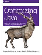
As an example, consider a performance test running against a group of backend Java web services that send and receive JSON. This type of test is very common when it is problematic to directly use the application frontend for load testing.
Figure 5-2 was generated from the JP GC extension pack for the Apache JMeter load-generation tool. In it, there are actually two systematic effects at work. The first is the linear pattern observed in the top line (the outlier service), which represents slow exhaustion of some limited server resource. This type of pattern is often associated with a memory leak, or some other resource being used and not released by a thread during request handling, and represents a candidate for investigation—it looks like it could be a genuine problem.
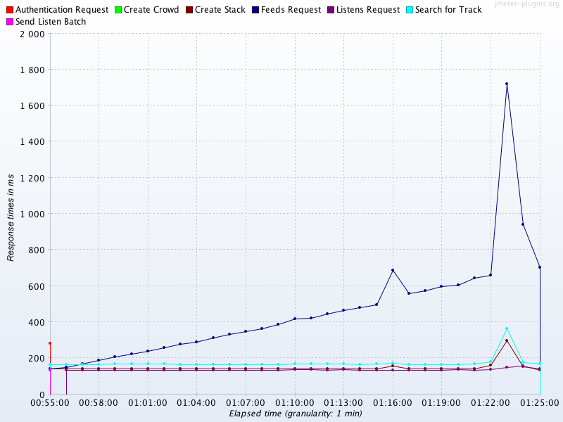
Figure 5-2. Systematic error
Note
Further analysis would be needed to confirm the type of resource that was being affected; we can’t just conclude that it’s a memory leak.
The second effect that should be noticed is the consistency of the majority of the other services at around the 180 ms level. This is suspicious, as the services are doing very different amounts of work in response to a request. So why are the results so consistent?
The answer is that while the services under test are located in London, this load test was conducted from Mumbai, India. The observed response time includes the irreducible round-trip network latency from Mumbai to London. This is in the range 120–150 ms, and so accounts for the vast majority of the observed time for the services other than the outlier.
This large, systematic effect is drowning out the differences in the actual response time (as the services are actually responding in much less than 120 ms). This is an example of a systematic error that does not represent a problem with our application. Instead, this error stems from a problem in our test setup, and the good news is that this artifact completely disappeared (as expected) when the test was rerun from London.
Random error
The case of random error deserves a mention here, although it is a very well-trodden path.
Note
The discussion assumes readers are familiar with basic statistical handling of normally distributed measurements (mean, mode, standard deviation, etc.); readers who aren’t should consult a basic textbook, such as The Handbook of Biological Statistics.1
Random errors are caused by unknown or unpredictable changes in the environment. In general scientific usage, these changes may occur in either the measuring instrument or the environment, but for software we assume that our measuring harness is reliable, and so the source of random error can only be the operating environment.
Random error is usually considered to obey a Gaussian (aka normal) distribution. A couple of typical examples are shown in Figure 5-3. The distribution is a good model for the case where an error is equally likely to make a positive or negative contribution to an observable, but as we will see, this is not a good fit for the JVM.
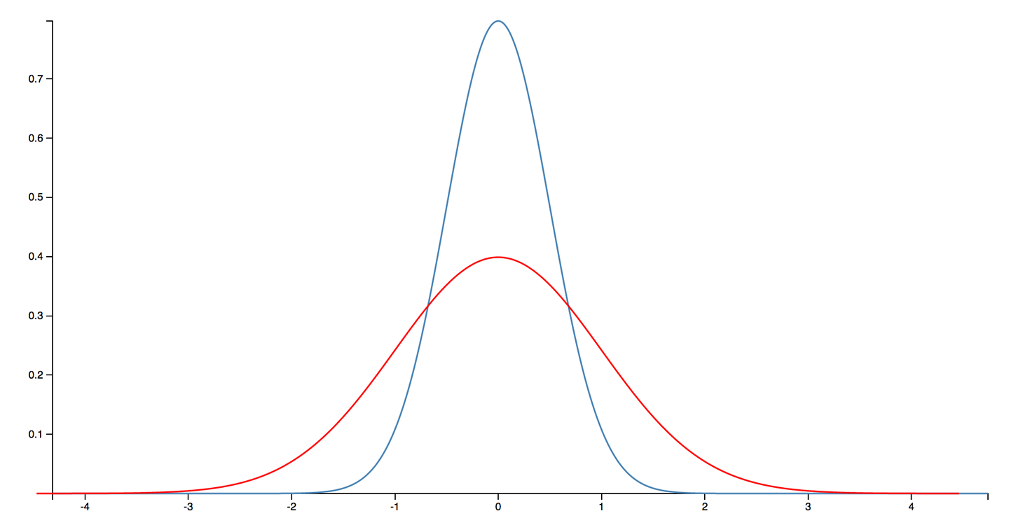
Figure 5-3. A Gaussian distribution (aka normal distribution or bell curve)
Spurious correlation
One of the most famous aphorisms about statistics is “correlation does not imply causation”—that is, just because two variables appear to behave similarly does not imply that there is an underlying connection between them.
In the most extreme examples, if a practitioner looks hard enough, then a correlation can be found between entirely unrelated measurements. For example, in Figure 5-4 we can see that consumption of chicken in the US is well correlated with total import of crude oil.2
Figure 5-4. A completely spurious correlation (Vigen)
These numbers are clearly not causally related; there is no factor that drives both the import of crude oil and the eating of chicken. However, it isn’t the absurd and ridiculous correlations that the practitioner needs to be wary of.
In Figure 5-5, we see the revenue generated by video arcades correlated to the number of computer science PhDs awarded. It isn’t too much of a stretch to imagine a sociological study that claimed a link between these observables, perhaps arguing that “stressed doctoral students were finding relaxation with a few hours of video games.” These types of claim are depressingly common, despite no such common factor actually existing.
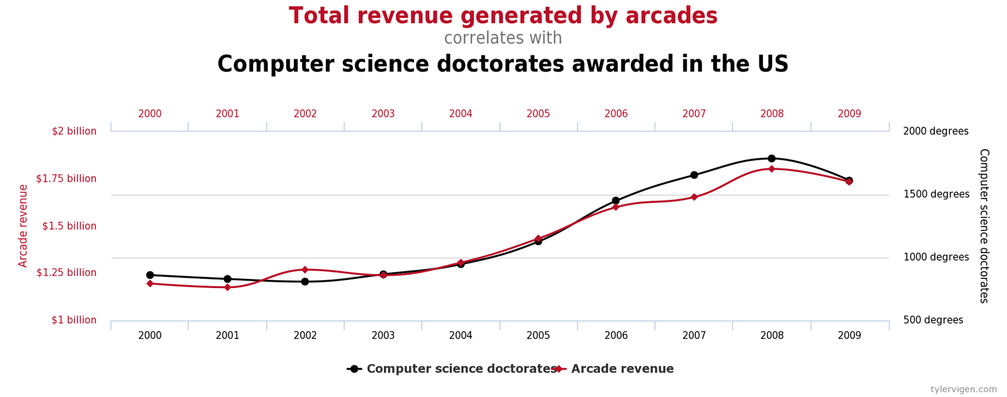
Figure 5-5. A less spurious correlation? (Vigen)
In the realm of the JVM and performance analysis, we need to be especially careful not to attribute a causal relationship between measurements based solely on correlation and that the connection “seems plausible.” This can be seen as one aspect of Feynman’s “you must not fool yourself” maxim.
We’ve met some examples of sources of error and mentioned the notorious bear trap of spurious correlation, so let’s move on to discuss an aspect of JVM performance measurement that requires some special care and attention to detail.
Non-Normal Statistics
Statistics based on the normal distribution do not require much mathematical sophistication. For this reason, the standard approach to statistics that is typically taught at pre-college or undergraduate level focuses heavily on the analysis of normally distributed data.
Students are taught to calculate the mean and the standard deviation (or variance), and sometimes higher moments, such as skew and kurtosis. However, these techniques have a serious drawback, in that the results can easily become distorted if the distribution has even a few far-flung outlying points.
Note
In Java performance, the outliers represent slow transactions and unhappy customers. We need to pay special attention to these points, and avoid techniques that dilute the importance of outliers.
To consider it from another viewpoint: unless a large number of customers are already complaining, it is unlikely that improving the average response time is the goal. For sure, doing so will improve the experience for everyone, but it is far more usual for a few disgruntled customers to be the cause of a latency tuning exercise. This implies that the outlier events are likely to be of more interest than the experience of the majority who are receiving satisfactory service.
In Figure 5-6 we can see a more realistic curve for the likely distribution of method (or transaction) times. It is clearly not a normal distribution.
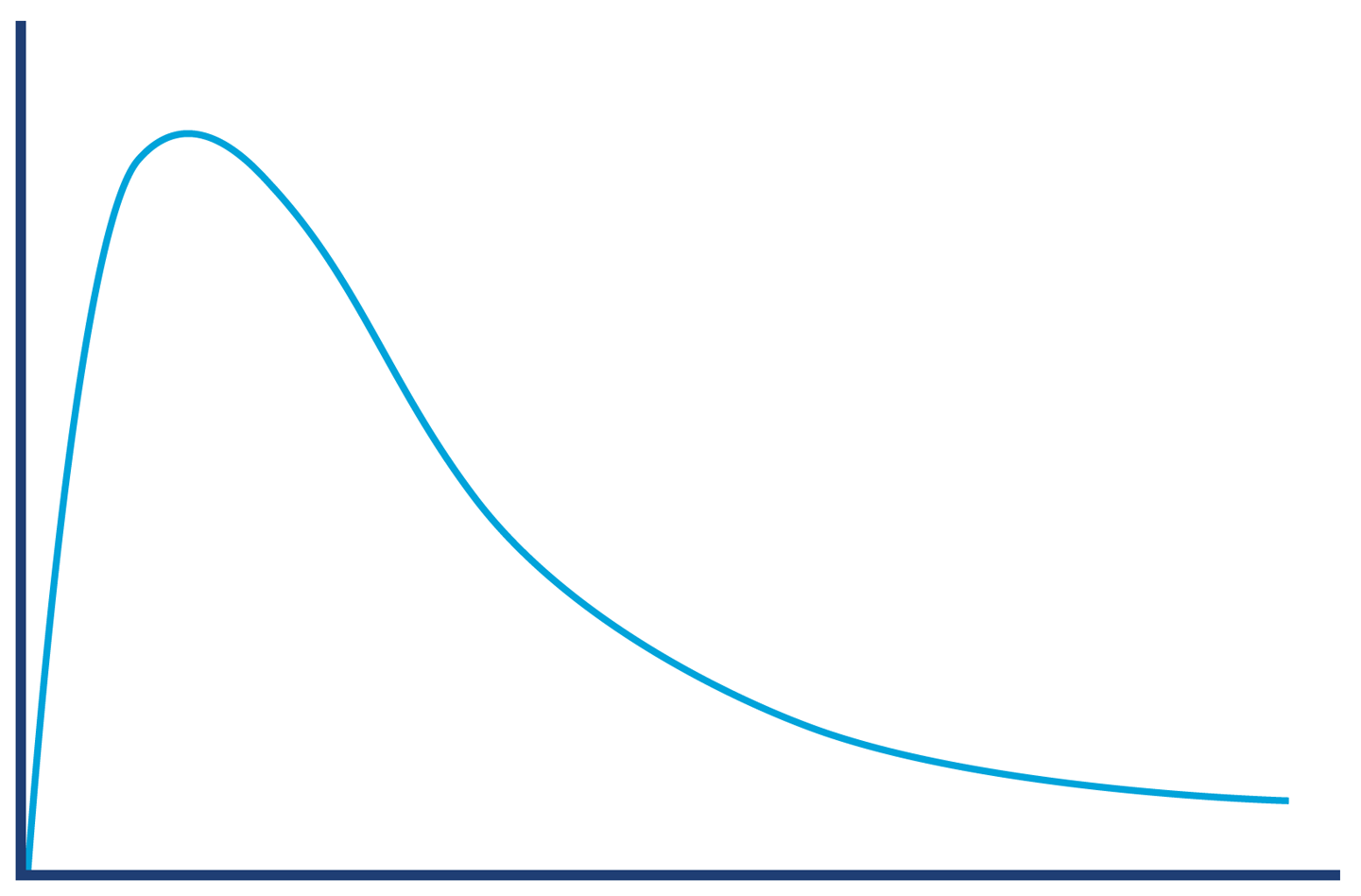
Figure 5-6. A more realistic view of the distribution of transaction times
The shape of the distribution in Figure 5-6 shows something that we know intuitively about the JVM: it has “hot paths” where all the relevant code is already JIT-compiled, there are no GC cycles, and so on. These represent a best-case scenario (albeit a common one); there simply are no calls that are randomly a bit faster.
This violates a fundamental assumption of Gaussian statistics and forces us to consider distributions that are non-normal.
Note
For distributions that are non-normal, many “basic rules” of normally distributed statistics are violated. In particular, standard deviation/variance and other higher moments are basically useless.
One technique that is very useful for handling the non-normal, “long-tail” distributions that the JVM produces is to use a modified scheme of percentiles. Remember that a distribution is a whole graph—it is a shape of data, and is not represented by a single number.
Instead of computing just the mean, which tries to express the whole distribution in a single result, we can use a sampling of the distribution at intervals. When used for normally distributed data, the samples are usually taken at regular intervals. However, a small adaptation means that the technique can be used for JVM statistics.
The modification is to use a sampling that takes into account the long-tail distribution by starting from the mean, then the 90th percentile, and then moving out logarithmically, as shown in the following method timing results. This means that we’re sampling according to a pattern that better corresponds to the shape of the data:
50.0% level was 23 ns
90.0% level was 30 ns
99.0% level was 43 ns
99.9% level was 164 ns
99.99% level was 248 ns
99.999% level was 3,458 ns
99.9999% level was 17,463 ns
The samples show us that while the average time was 23 ns to execute a getter method, for 1 request in 1,000 the time was an order of magnitude worse, and for 1 request in 100,000 it was two orders of magnitude worse than average.
Long-tail distributions can also be referred to as high dynamic range distributions. The dynamic range of an observable is usually defined as the maximum recorded value divided by the minimum (assuming it’s nonzero).
Logarithmic percentiles are a useful simple tool for understanding the long tail. However, for more sophisticated analysis, we can use a public domain library for handling datasets with high dynamic range. The library is called HdrHistogram and is available from GitHub. It was originally created by Gil Tene (Azul Systems), with additional work by Mike Barker, Darach Ennis, and Coda Hale.
Note
A histogram is a way of summarizing data by using a finite set of ranges (called buckets) and displaying how often data falls into each bucket.
HdrHistogram is also available on Maven Central. At the time of writing, the current version is 2.1.9, and you can add it to your projects by adding this dependency stanza to pom.xml:
<dependency><groupId>org.hdrhistogram</groupId><artifactId>HdrHistogram</artifactId><version>2.1.9</version></dependency>
Let’s look at a simple example using HdrHistogram. This example takes in a file of numbers and computes the HdrHistogram for the difference between successive results:
publicclassBenchmarkWithHdrHistogram{privatestaticfinallongNORMALIZER=1_000_000;privatestaticfinalHistogramHISTOGRAM=newHistogram(TimeUnit.MINUTES.toMicros(1),2);publicstaticvoidmain(String[]args)throwsException{finalList<String>values=Files.readAllLines(Paths.get(args[0]));doublelast=0;for(finalStringtVal:values){doubleparsed=Double.parseDouble(tVal);doublegcInterval=parsed-last;last=parsed;HISTOGRAM.recordValue((long)(gcInterval*NORMALIZER));}HISTOGRAM.outputPercentileDistribution(System.out,1000.0);}}
The output shows the times between successive garbage collections. As we’ll see in Chapters 6 and 8, GC does do not occur at regular intervals, and understanding the distribution of how frequently it occurs could be useful. Here’s what the histogram plotter produces for a sample GC log:
       Value     Percentile TotalCount 1/(1-Percentile)

       14.02 0.000000000000          1           1.00
     1245.18 0.100000000000         37           1.11
     1949.70 0.200000000000         82           1.25
     1966.08 0.300000000000        126           1.43
     1982.46 0.400000000000        157           1.67

...

    28180.48 0.996484375000        368         284.44
    28180.48 0.996875000000        368         320.00
    28180.48 0.997265625000        368         365.71
    36438.02 0.997656250000        369         426.67
    36438.02 1.000000000000        369
#[Mean    =      2715.12, StdDeviation   =      2875.87]
#[Max     =     36438.02, Total count    =          369]
#[Buckets =           19, SubBuckets     =          256]
The raw output of the formatter is rather hard to analyze, but fortunately, the HdrHistogram project includes an online formatter that can be used to generate visual histograms from the raw output.
For this example, it produces output like that shown in Figure 5-7.
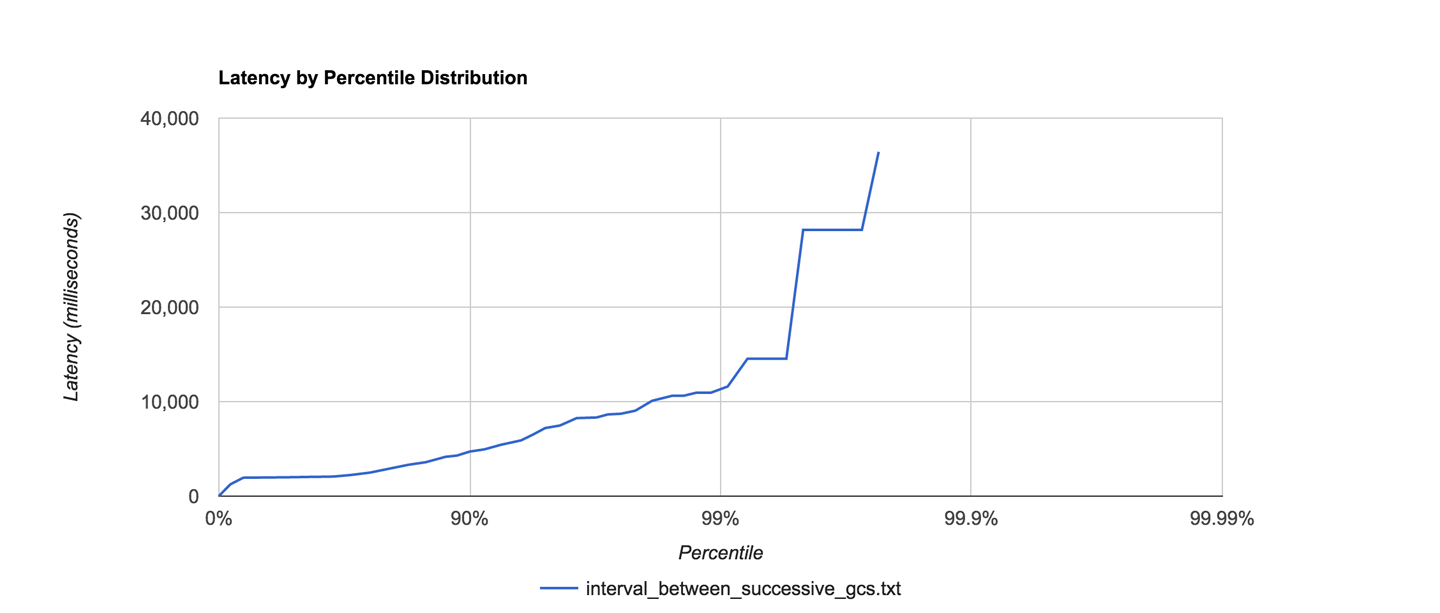
Figure 5-7. Example HdrHistogram visualization
For many observables that we wish to measure in Java performance tuning, the statistics are often highly non-normal, and HdrHistogram can be a very useful tool in helping to understand and visualize the shape of the data.
Interpretation of Statistics
Empirical data and observed results do not exist in a vacuum, and it is quite common that one of the hardest jobs lies in interpreting the results that we obtain from measuring our applications.
No matter what they tell you, it’s always a people problem.
Gerald Weinberg
In Figure 5-8 we show an example memory allocation rate for a real Java application. This example is for a reasonably well-performing application. The screenshot comes from the Censum garbage collection analyzer, which we will meet in Chapter 8.
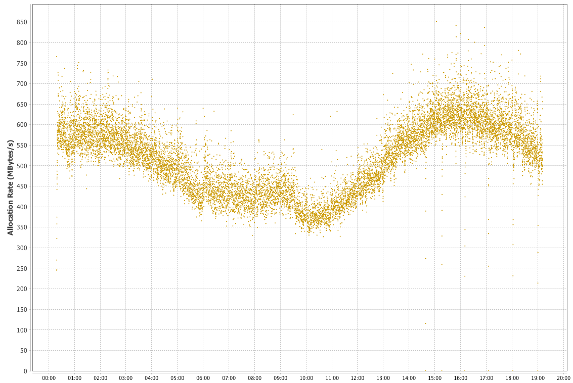
Figure 5-8. Example allocation rate
The interpretation of the allocation data is relatively straightforward, as there is a clear signal present. Over the time period covered (almost a day), allocation rates were basically stable between 350 and 700 MB per second. There is a downward trend starting approximately 5 hours after the JVM started up, and a clear minimum between 9 and 10 hours, after which the allocation rate starts to rise again.
These types of trends in observables are very common, as the allocation rate will usually reflect the amount of work an application is actually doing, and this will vary widely depending on the time of day. However, when we are interpreting real observables, the picture can rapidly become more complicated. This can lead to what is sometimes called the “Hat/Elephant” problem, after a passage in The Little Prince by Antoine de Saint-Exupéry.
The problem is illustrated by Figure 5-9. All we can initially see is a complex histogram of HTTP request-response times. However, just like the narrator of the book, if we can imagine or analyze a bit more, we can see that the complex picture is actually made up of several fairly simple pieces.
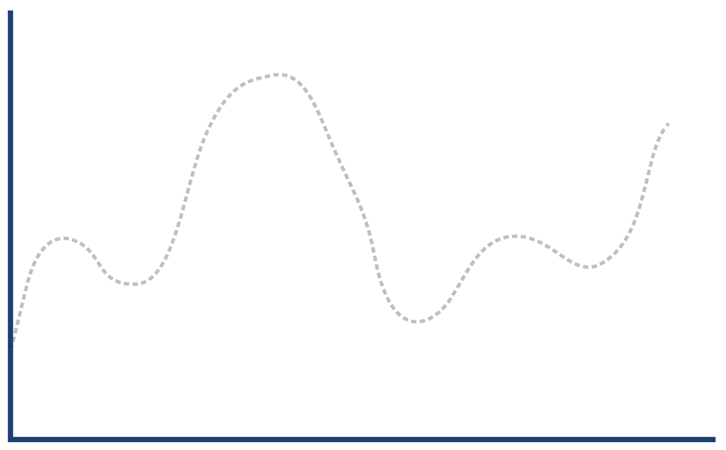
Figure 5-9. Hat, or elephant eaten by a boa?
The key to decoding the response histogram is to realize that “web application responses” is a very general category, including successful requests (so-called 2xx responses), client errors (4xx, including the ubiquitous 404 error), and server errors (5xx, especially 500 Internal Server Error).
Each type of response has a different characteristic distribution for response times. If a client makes a request for a URL that has no mapping (a 404), then the web server can immediately reply with a response. This means that the histogram for only client error responses looks more like Figure 5-10.
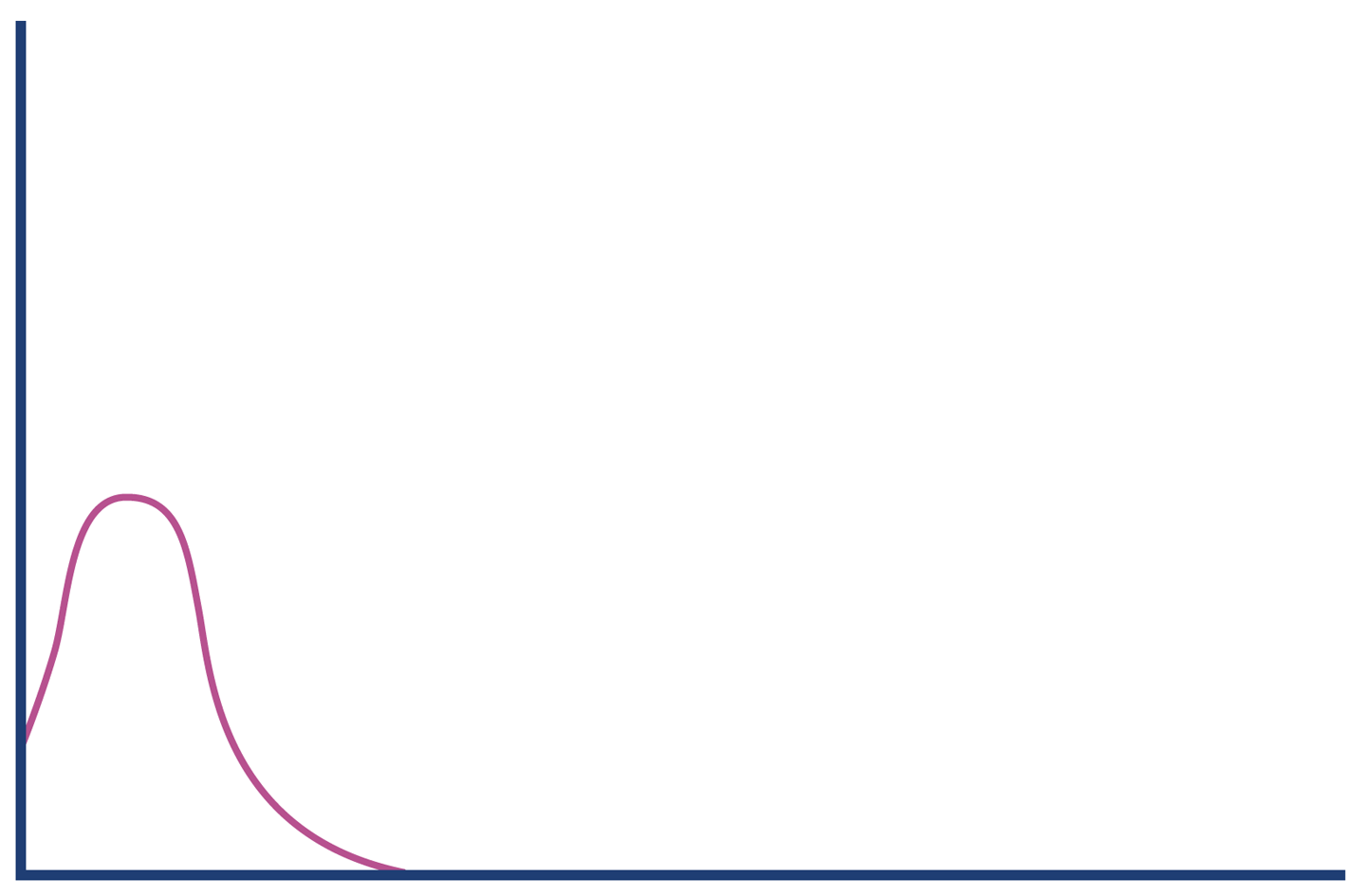
Figure 5-10. Client errors
By contrast, server errors often occur after a large amount of processing time has been expended (for example, due to backend resources being under stress or timing out). So, the histogram for server error responses might look like Figure 5-11.
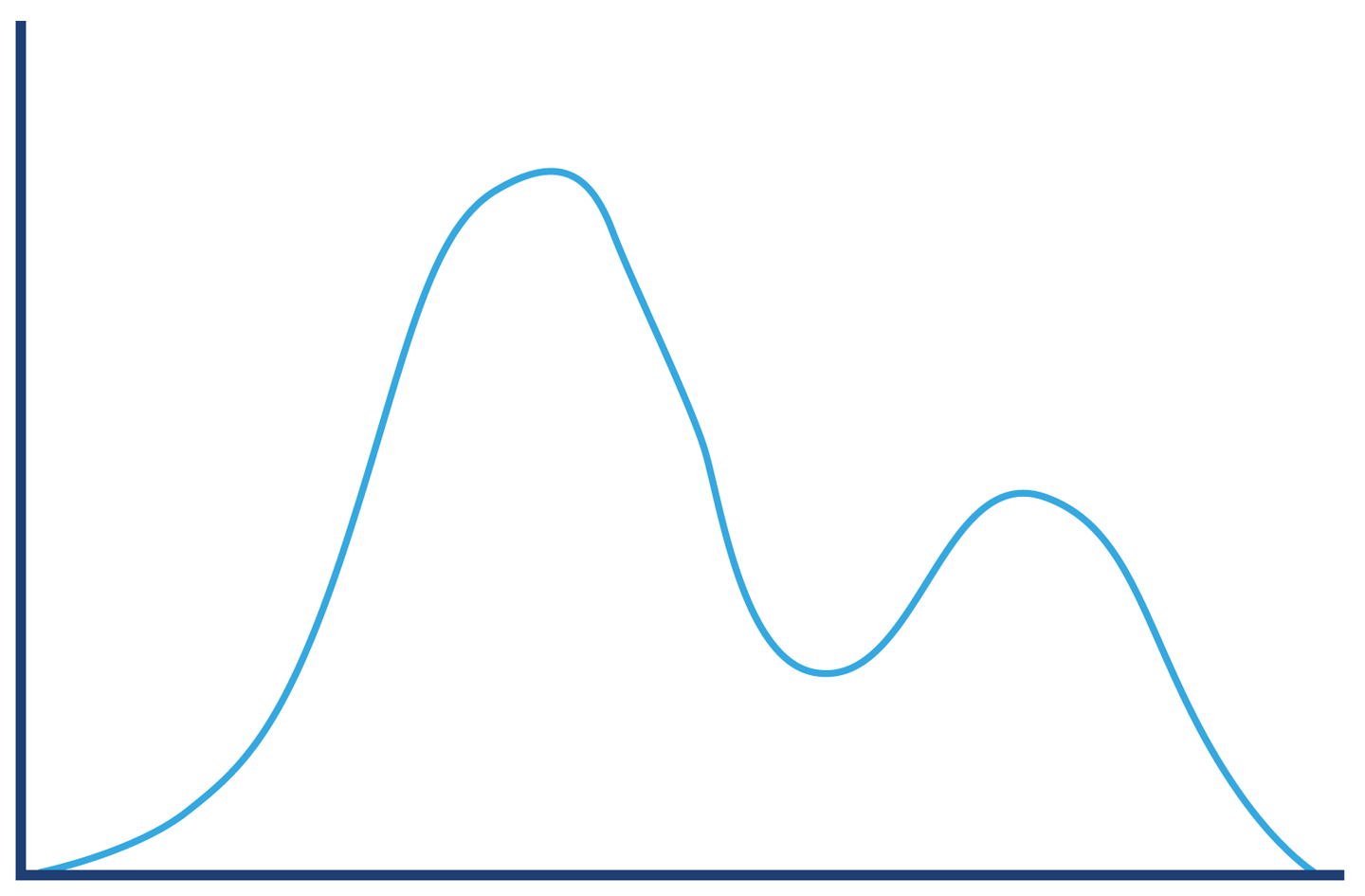
Figure 5-11. Server errors
The successful requests will have a long-tail distribution, but in reality we may expect the response distribution to be “multimodal” and have several local maxima. An example is shown in Figure 5-12, and represents the possibility that there could be two common execution paths through the application with quite different response times.
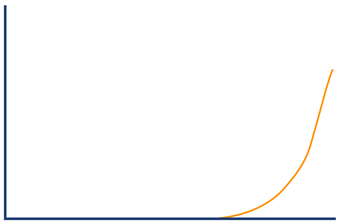
Figure 5-12. Successful requests
Combining these different types of responses into a single graph results in the structure shown in Figure 5-13. We have rederived our original “hat” shape from the separate histograms.
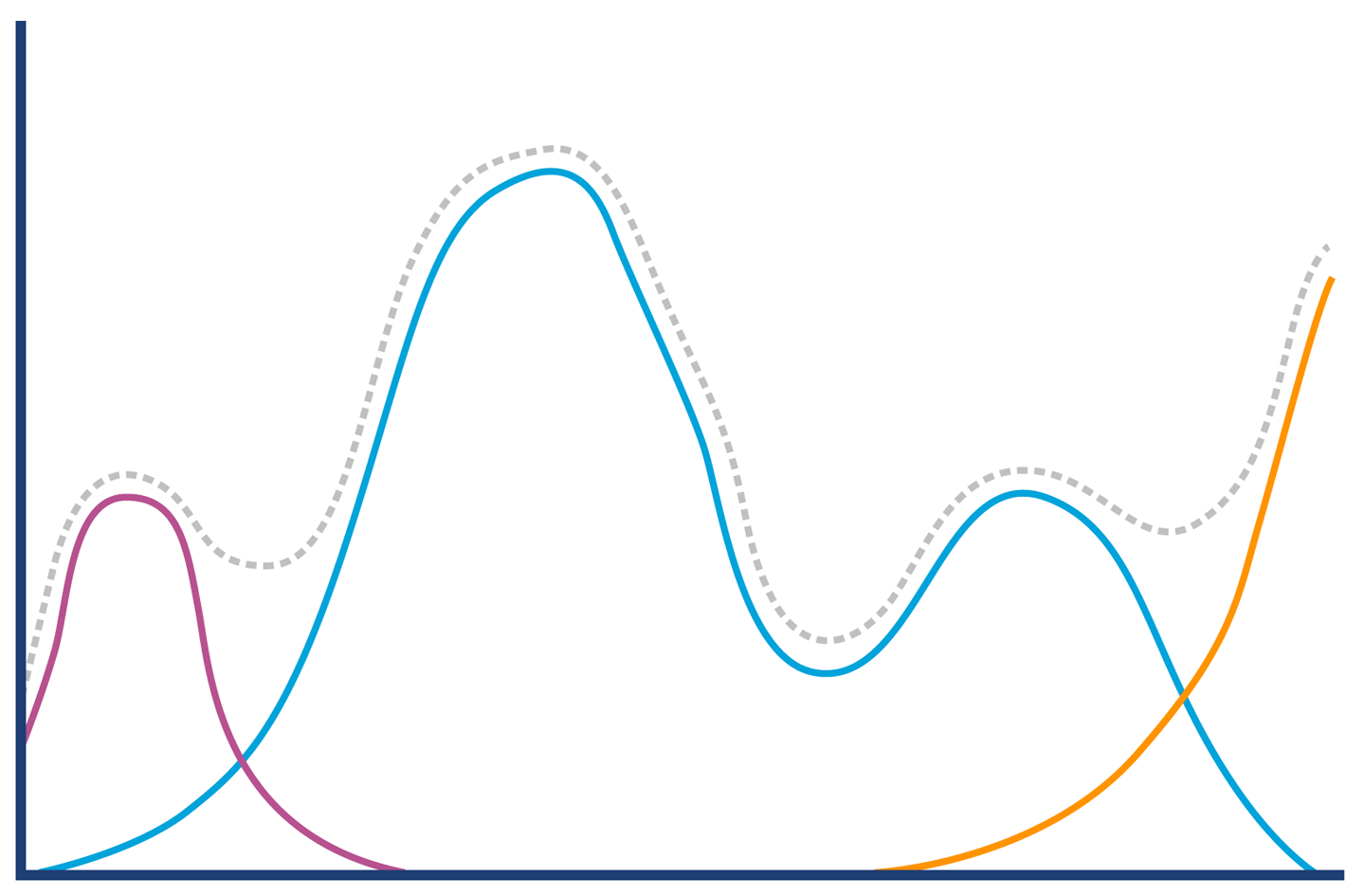
Figure 5-13. Hat or elephant revisited
The concept of breaking down a general observable into more meaningful sub-populations is a very useful one, and shows that we need to make sure that we understand our data and domain well enough before trying to infer conclusions from our results. We may well want to further break down our data into smaller sets; for example, the successful requests may have very different distributions for requests that are predominantly read, as opposed to requests that are updates or uploads.
The engineering team at PayPal have written extensively about their use of statistics and analysis; they have a blog that contains excellent resources. In particular, the piece “Statistics for Software” by Mahmoud Hashemi is a great introduction to their methodologies, and includes a version of the Hat/Elephant problem discussed earlier.
Summary
Microbenchmarking is the closest that Java performance comes to a “Dark Art.” While this characterization is evocative, it is not wholly deserved. It is still an engineering discipline undertaken by working developers. However, microbenchmarks should be used with caution:
-
Do not microbenchmark unless you know you are a known use case for it.
-
If you must microbenchmark, use JMH.
-
Discuss your results as publicly as you can, and in the company of your peers.
-
Be prepared to be wrong a lot and to have your thinking challenged repeatedly.
One of the positive aspects of working with microbenchmarks is that it exposes the highly dynamic behavior and non-normal distributions that are produced by low-level subsystems. This, in turn, leads to a better understanding and mental models of the complexities of the JVM.
In the next chapter, we will move on from methodology and start our technical deep dive into the JVM’s internals and major subsystems, by beginning our examination of garbage collection.
1 John H. McDonald, Handbook of Biological Statistics, 3rd ed. (Baltimore, MD: Sparky House Publishing, 2014).
2 The spurious correlations in this section come from Tyler Vigen’s site and are reused here with permission under a Creative Commons license. If you enjoy them, Vigen has a book with many more amusing examples, available from the link.