Table of Contents for
Optimizing Java
 Optimizing Java
Published by
O'Reilly Media, Inc., 2018
Optimizing Java
Published by
O'Reilly Media, Inc., 2018
- nav
- Cover
- Optimizing Java
- Optimizing Java
- Dedication
- Foreword
- Preface
- 1. Optimization and Performance Defined
- 2. Overview of the JVM
- 3. Hardware and Operating Systems
- 4. Performance Testing Patterns and Antipatterns
- 5. Microbenchmarking and Statistics
- 6. Understanding Garbage Collection
- 7. Advanced Garbage Collection
- 8. GC Logging, Monitoring, Tuning, and Tools
- 9. Code Execution on the JVM
- 10. Understanding JIT Compilation
- 11. Java Language Performance Techniques
- 12. Concurrent Performance Techniques
- 13. Profiling
- 14. High-Performance Logging and Messaging
- 15. Java 9 and the Future
- Index
- About the Authors
- Colophon
Chapter 3. Hardware and Operating Systems
Why should Java developers care about hardware?
For many years the computer industry has been driven by Moore’s Law, a hypothesis made by Intel founder Gordon Moore about long-term trends in processor capability. The law (really an observation or extrapolation) can be framed in a variety of ways, but one of the most usual is:
The number of transistors on a mass-produced chip roughly doubles every 18 months.
This phenomenon represents an exponential increase in computer power over time. It was originally cited in 1965, so represents an incredible long-term trend, almost unparalleled in the history of human development. The effects of Moore’s Law have been transformative in many (if not most) areas of the modern world.
Note
The death of Moore’s Law has been repeatedly proclaimed for decades now. However, there are very good reasons to suppose that, for all practical purposes, this incredible progress in chip technology has (finally) come to an end.
Hardware has become increasingly complex in order to make good use of the “transistor budget” available in modern computers. The software platforms that run on that hardware have also increased in complexity to exploit the new capabilities, so while software has far more power at its disposal it has come to rely on complex underpinnings to access that performance increase.
The net result of this huge increase in the performance available to the ordinary application developer has been the blossoming of complex software. Software applications now pervade every aspect of global society.
Or, to put it another way:
Software is eating the world.
Marc Andreessen
As we will see, Java has been a beneficiary of the increasing amount of computer power. The design of the language and runtime has been well suited (or lucky) to make use of this trend in processor capability. However, the truly performance-conscious Java programmer needs to understand the principles and technology that underpin the platform in order to make best use of the available resources.
In later chapters, we will explore the software architecture of modern JVMs and techniques for optimizing Java applications at the platform and code levels. But before turning to those subjects, let’s take a quick look at modern hardware and operating systems, as an understanding of those subjects will help with everything that follows.
Introduction to Modern Hardware
Many university courses on hardware architectures still teach a simple-to-understand, classical view of hardware. This “motherhood and apple pie” view of hardware focuses on a simple view of a register-based machine, with arithmetic, logic, and load and store operations. As a result, it overemphasizes C programming as the source of truth as compared to what a CPU actually does. This is, simply, a factually incorrect worldview in modern times.
Since the 1990s the world of the application developer has, to a large extent, revolved around the Intel x86/x64 architecture. This is an area of technology that has undergone radical change, and many advanced features now form important parts of the landscape. The simple mental model of a processor’s operation is now completely incorrect, and intuitive reasoning based on it is liable to lead to utterly wrong conclusions.
To help address this, in this chapter, we will discuss several of these advances in CPU technology. We will start with the behavior of memory, as this is by far the most important to a modern Java developer.
Memory
As Moore’s Law advanced, the exponentially increasing number of transistors was initially used for faster and faster clock speed. The reasons for this are obvious: faster clock speed means more instructions completed per second. Accordingly, the speed of processors has advanced hugely, and the 2+ GHz processors that we have today are hundreds of times faster than the original 4.77 MHz chips found in the first IBM PC.
However, the increasing clock speeds uncovered another problem. Faster chips require a faster stream of data to act upon. As Figure 3-1 shows,1 over time main memory could not keep up with the demands of the processor core for fresh data.

Figure 3-1. Speed of memory and transistor counts (Hennessy and Patterson, 2011)
This results in a problem: if the CPU is waiting for data, then faster cycles don’t help, as the CPU will just have to idle until the required data arrives.
Memory Caches
To solve this problem, CPU caches were introduced. These are memory areas on the CPU that are slower than CPU registers, but faster than main memory. The idea is for the CPU to fill the cache with copies of often-accessed memory locations rather than constantly having to re-address main memory.
Modern CPUs have several layers of cache, with the most-often-accessed caches being located close to the processing core. The cache closest to the CPU is usually called L1 (for “level 1 cache”), with the next being referred to as L2, and so on. Different processor architectures have a varying number and configuration of caches, but a common choice is for each execution core to have a dedicated, private L1 and L2 cache, and an L3 cache that is shared across some or all of the cores. The effect of these caches in speeding up access times is shown in Figure 3-2.2
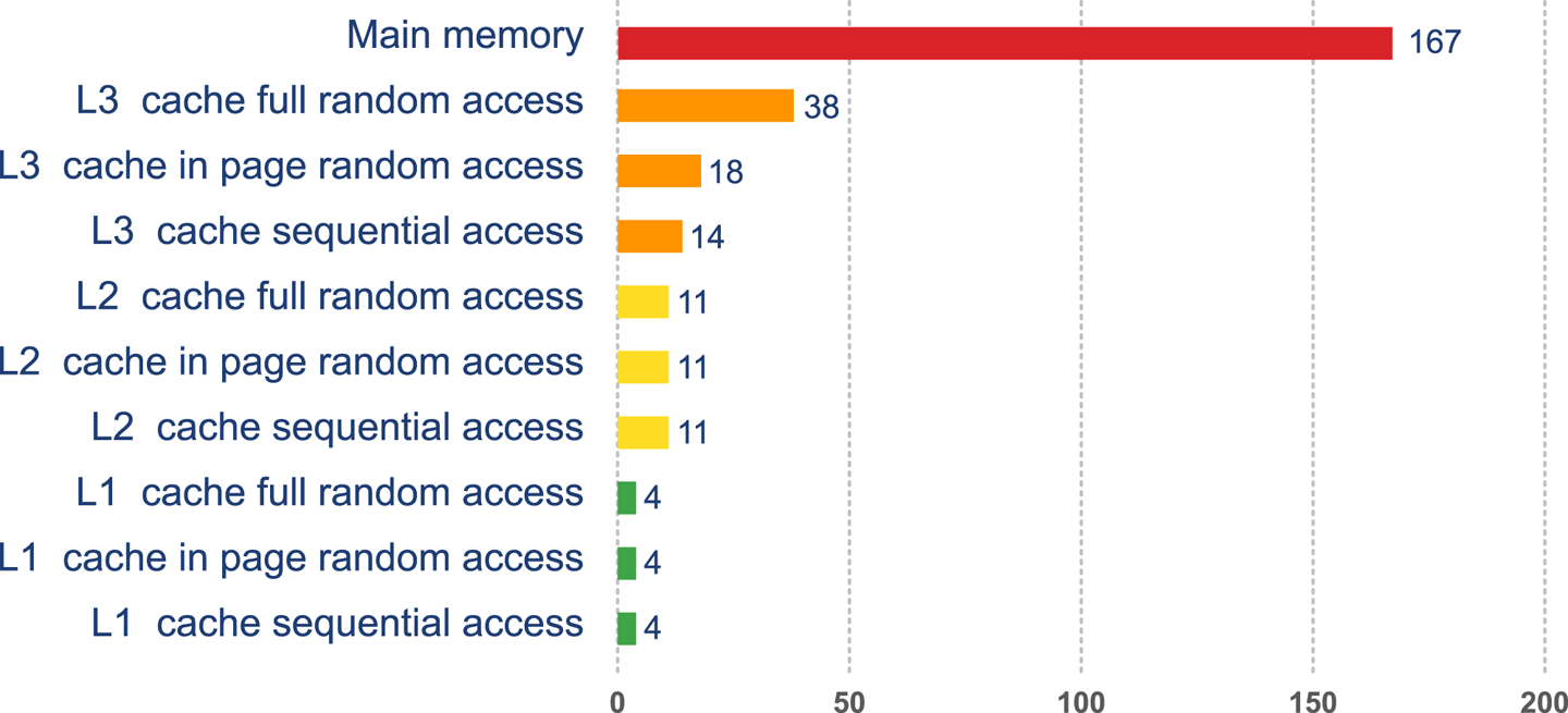
Figure 3-2. Access times for various types of memory
This approach to cache architecture improves access times and helps keep the core fully stocked with data to operate on. Due to the clock speed versus access time gap, more transistor budget is devoted to caches on a modern CPU.
The resulting design can be seen in Figure 3-3. This shows the L1 and L2 caches (private to each CPU core) and a shared L3 cache that is common to all cores on the CPU. Main memory is accessed over the Northbridge component, and it is traversing this bus that causes the large drop-off in access time to main memory.
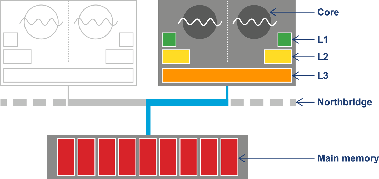
Figure 3-3. Overall CPU and memory architecture
Although the addition of a caching architecture hugely improves processor throughput, it introduces a new set of problems. These problems include determining how memory is fetched into and written back from the cache. The solutions to this problem are usually referred to as cache consistency protocols.
Note
There are other problems that crop up when this type of caching is applied in a parallel processing environment, as we will see later in this book.
At the lowest level, a protocol called MESI (and its variants) is commonly found on a wide range of processors. It defines four states for any line in a cache. Each line (usually 64 bytes) is either:
-
Modified (but not yet flushed to main memory)
-
Exclusive (present only in this cache, but does match main memory)
-
Shared (may also be present in other caches; matches main memory)
-
Invalid (may not be used; will be dropped as soon as practical)
The idea of the protocol is that multiple processors can simultaneously be in the Shared state. However, if a processor transitions to any of the other valid states (Exclusive or Modified), then this will force all the other processors into the Invalid state. This is shown in Table 3-1.
| M | E | S | I | |
|---|---|---|---|---|
M |
- |
- |
- |
Y |
E |
- |
- |
- |
Y |
S |
- |
- |
Y |
Y |
I |
Y |
Y |
Y |
Y |
The protocol works by broadcasting the intention of a processor to change state. An electrical signal is sent across the shared memory bus, and the other processors are made aware. The full logic for the state transitions is shown in Figure 3-4.
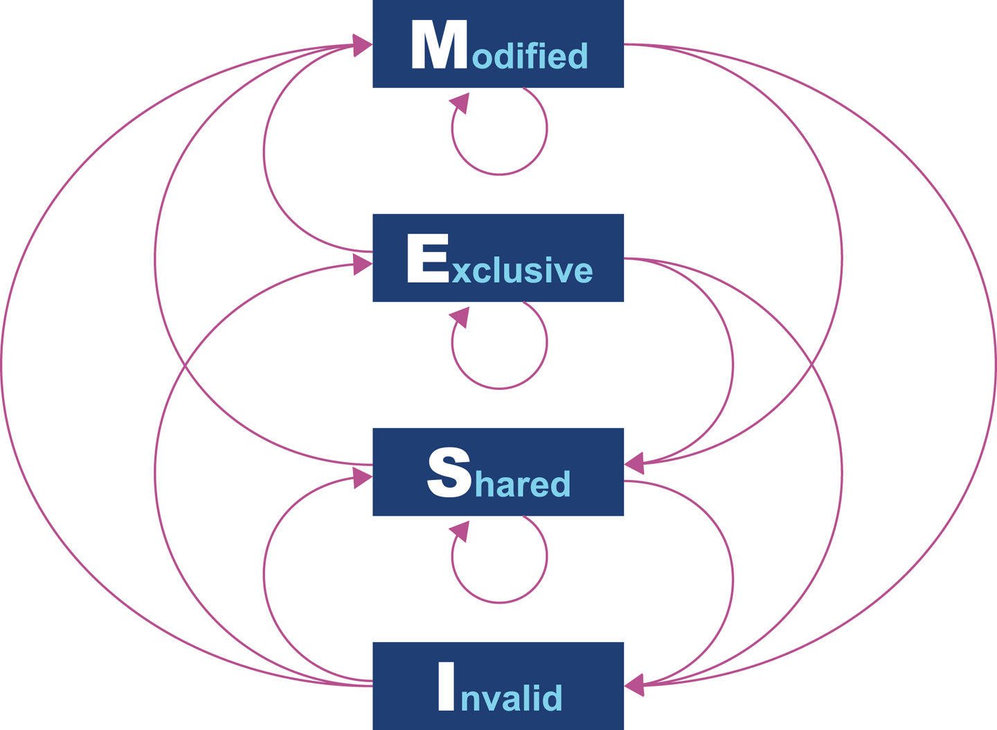
Figure 3-4. MESI state transition diagram
Originally, processors wrote every cache operation directly into main memory. This was called write-through behavior, but it was and is very inefficient, and required a large amount of bandwidth to memory. More recent processors also implement write-back behavior, where traffic back to main memory is significantly reduced by processors writing only modified (dirty) cache blocks to memory when the cache blocks are replaced.
The overall effect of caching technology is to greatly increase the speed at which data can be written to, or read from, memory. This is expressed in terms of the bandwidth to memory. The burst rate, or theoretical maximum, is based on several factors:
-
Clock frequency of memory
-
Width of the memory bus (usually 64 bits)
-
Number of interfaces (usually two in modern machines)
This is multiplied by two in the case of DDR RAM (DDR stands for “double data rate” as it communicates on both edges of a clock signal). Applying the formula to 2015 commodity hardware gives a theoretical maximum write speed of 8–12 GB/s. In practice, of course, this could be limited by many other factors in the system. As it stands, this gives a modestly useful value to allow us to see how close the hardware and software can get.
Let’s write some simple code to exercise the cache hardware, as seen in Example 3-1.
Example 3-1. Caching example
publicclassCaching{privatefinalintARR_SIZE=2*1024*1024;privatefinalint[]testData=newint[ARR_SIZE];privatevoidrun(){System.err.println("Start: "+System.currentTimeMillis());for(inti=0;i<15_000;i++){touchEveryLine();touchEveryItem();}System.err.println("Warmup finished: "+System.currentTimeMillis());System.err.println("Item Line");for(inti=0;i<100;i++){longt0=System.nanoTime();touchEveryLine();longt1=System.nanoTime();touchEveryItem();longt2=System.nanoTime();longelItem=t2-t1;longelLine=t1-t0;doublediff=elItem-elLine;System.err.println(elItem+" "+elLine+" "+(100*diff/elLine));}}privatevoidtouchEveryItem(){for(inti=0;i<testData.length;i++)testData[i]++;}privatevoidtouchEveryLine(){for(inti=0;i<testData.length;i+=16)testData[i]++;}publicstaticvoidmain(String[]args){Cachingc=newCaching();c.run();}}
Intuitively, touchEveryItem() does 16 times as much work as
touchEveryLine(), as 16 times as many data items must be updated. However,
the point of this simple example is to show how badly intuition can lead us
astray when dealing with JVM performance. Let’s look at some sample output from
the Caching class, as shown in Figure 3-5.
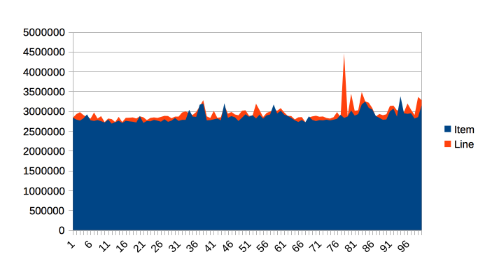
Figure 3-5. Time elapsed for Caching example
The graph shows 100 runs of each function, and is intended to show several different effects. Firstly, notice that the results for both functions are remarkably similar in terms of time taken, so the intuitive expectation of “16 times as much work” is clearly false.
Instead, the dominant effect of this code is to exercise the memory bus, by
transferring the contents of the array from main memory into the cache to
be operated on by touchEveryItem() and touchEveryLine().
In terms of the statistics of the numbers, although the results are reasonably consistent, there are individual outliers that are 30–35% different from the median value.
Overall, we can see that each iteration of the simple memory function takes around 3 milliseconds (2.86 ms on average) to traverse a 100 MB chunk of memory, giving an effective memory bandwidth of just under 3.5 GB/s. This is less than the theoretical maximum, but is still a reasonable number.
Note
Modern CPUs have a hardware prefetcher that can detect predictable patterns in data access (usually just a regular “stride” through the data). In this example, we’re taking advantage of that fact in order to get closer to a realistic maximum for memory access bandwidth.
One of the key themes in Java performance is the sensitivity of applications to object allocation rates. We will return to this point several times, but this simple example gives us a basic yardstick for how high allocation rates could rise.
Modern Processor Features
Hardware engineers sometimes refer to the new features that have become possible as a result of Moore’s Law as “spending the transistor budget.” Memory caches are the most obvious use of the growing number of transistors, but other techniques have also appeared over the years.
Translation Lookaside Buffer
One very important use is in a different sort of cache, the Translation Lookaside Buffer (TLB). This acts as a cache for the page tables that map virtual memory addresses to physical addresses, which greatly speeds up a very frequent operation—access to the physical address underlying a virtual address.
Note
There’s a memory-related software feature of the JVM that also has the acronym TLB (as we’ll see later). Always check which feature is being discussed when you see TLB mentioned.
Without the TLB, all virtual address lookups would take 16 cycles, even if the page table was held in the L1 cache. Performance would be unacceptable, so the TLB is basically essential for all modern chips.
Branch Prediction and Speculative Execution
One of the advanced processor tricks that appear on modern processors is branch prediction. This is used to prevent the processor from having to wait to evaluate a value needed for a conditional branch. Modern processors have multistage instruction pipelines. This means that the execution of a single CPU cycle is broken down into a number of separate stages. There can be several instructions in flight (at different stages of execution) at once.
In this model a conditional branch is problematic, because until the condition is evaluated, it isn’t known what the next instruction after the branch will be. This can cause the processor to stall for a number of cycles (in practice, up to 20), as it effectively empties the multistage pipeline behind the branch.
Note
Speculative execution was, famously, the cause of major security problems discovered to affect very large numbers of CPUs in early 2018.
To avoid this, the processor can dedicate transistors to building up a heuristic to decide which branch is more likely to be taken. Using this guess, the CPU fills the pipeline based on a gamble. If it works, then the CPU carries on as though nothing had happened. If it’s wrong, then the partially executed instructions are dumped, and the CPU has to pay the penalty of emptying the pipeline.
Hardware Memory Models
The core question about memory that must be answered in a multicore system is “How can multiple different CPUs access the same memory location consistently?”
The answer to this question is highly hardware-dependent, but in general, javac, the JIT compiler, and the CPU are all allowed to make changes to the order in which code executes.
This is subject to the provision that any changes don’t affect the outcome as observed by the current thread.
For example, let’s suppose we have a piece of code like this:
myInt=otherInt;intChanged=true;
There is no code between the two assignments, so the executing thread doesn’t need to care about what order they happen in, and thus the environment is at liberty to change the order of instructions.
However, this could mean that in another thread that has visibility of these data items, the order could change, and the value of myInt read by the other thread could be the old value, despite intChanged being seen to be true.
This type of reordering (stores moved after stores) is not possible on x86 chips, but as Table 3-2 shows, there are other architectures where it can, and does, happen.
| ARMv7 | POWER | SPARC | x86 | AMD64 | zSeries | |
|---|---|---|---|---|---|---|
Loads moved after loads |
Y |
Y |
- |
- |
- |
- |
Loads moved after stores |
Y |
Y |
- |
- |
- |
- |
Stores moved after stores |
Y |
Y |
- |
- |
- |
- |
Stores moved after loads |
Y |
Y |
Y |
Y |
Y |
Y |
Atomic moved with loads |
Y |
Y |
- |
- |
- |
- |
Atomic moved with stores |
Y |
Y |
- |
- |
- |
- |
Incoherent instructions |
Y |
Y |
Y |
Y |
- |
Y |
In the Java environment, the Java Memory Model (JMM) is explicitly designed to be a weak model to take into account the differences in consistency of memory access between processor types. Correct use of locks and volatile access is a major part of ensuring that multithreaded code works properly. This is a very important topic that we will return to in Chapter 12.
There has been a trend in recent years for software developers to seek greater understanding of the workings of hardware in order to derive better performance. The term mechanical sympathy has been coined by Martin Thompson and others to describe this approach, especially as applied to the low-latency and high-performance spaces. It can be seen in recent research into lock-free algorithms and data structures, which we will meet toward the end of the book.
Operating Systems
The point of an operating system is to control access to resources that must be shared between multiple executing processes. All resources are finite, and all processes are greedy, so the need for a central system to arbitrate and meter access is essential. Among these scarce resources, the two most important are usually memory and CPU time.
Virtual addressing via the memory management unit (MMU) and its page tables is the key feature that enables access control of memory, and prevents one process from damaging the memory areas owned by another.
The TLBs that we met earlier in the chapter are a hardware feature that improves lookup times to physical memory. The use of the buffers improves performance for software’s access time to memory. However, the MMU is usually too low-level for developers to directly influence or be aware of. Instead, let’s take a closer look at the OS process scheduler, as this controls access to the CPU and is a far more user-visible piece of the operating system kernel.
The Scheduler
Access to the CPU is controlled by the process scheduler. This uses a queue known as the run queue as a waiting area for threads or processes that are eligible to run but which must wait their turn for the CPU. On a modern system there are effectively always more threads/processes that want to run than can, and so this CPU contention requires a mechanism to resolve it.
The job of the scheduler is to respond to interrupts, and to manage access to the CPU cores. The lifecycle of a Java thread is shown in Figure 3-6. In theory, the Java specification permits threading models whereby Java threads do not necessarily correspond to operating system threads. However, in practice, such “green threads” approaches have not proved to be useful, and have been abandoned in mainstream operating environments.
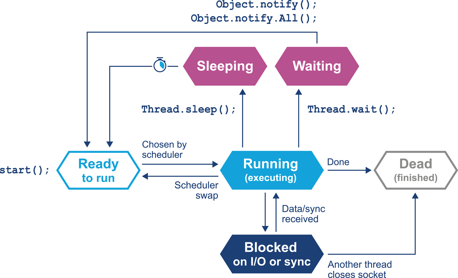
Figure 3-6. Thread lifecycle
In this relatively simple view, the OS scheduler moves threads on and off the single core in the system. At the end of the time quantum (often 10 ms or 100 ms in older operating systems), the scheduler moves the thread to the back of the run queue to wait until it reaches the front of the queue and is eligible to run again.
If a thread wants to voluntarily give up its time quantum it can do so either
for a fixed amount of time (via sleep()) or until a condition is met (using
wait()). Finally, a thread can also block on I/O or a software lock.
When you are meeting this model for the first time, it may help to think about a machine that has only a single execution core. Real hardware is, of course, more complex, and virtually any modern machine will have multiple cores, which allows for true simultaneous execution of multiple execution paths. This means that reasoning about execution in a true multiprocessing environment is very complex and counterintuitive.
An often-overlooked feature of operating systems is that by their nature, they introduce periods of time when code is not running on the CPU. A process that has completed its time quantum will not get back on the CPU until it arrives at the front of the run queue again. Combined with the fact that CPU is a scarce resource, this means that code is waiting more often than it is running.
This means that the statistics we want to generate from processes that we actually want to observe are affected by the behavior of other processes on the systems. This “jitter” and the overhead of scheduling is a primary cause of noise in observed results. We will discuss the statistical properties and handling of real results in Chapter 5.
One of the easiest ways to see the action and behavior of a scheduler is to try to observe the overhead imposed by the OS to achieve scheduling. The following code executes 1,000 separate 1 ms sleeps. Each of these sleeps will involve the thread being sent to the back of the run queue, and having to wait for a new time quantum. So, the total elapsed time of the code gives us some idea of the overhead of scheduling for a typical process:
longstart=System.currentTimeMillis();for(inti=0;i<2_000;i++){Thread.sleep(2);}longend=System.currentTimeMillis();System.out.println("Millis elapsed: "+(end-start)/4000.0);
Running this code will cause wildly divergent results, depending on the operating system. Most Unixes will report roughly 10–20% overhead. Earlier versions of Windows had notoriously bad schedulers, with some versions of Windows XP reporting up to 180% overhead for scheduling (so that 1,000 sleeps of 1 ms would take 2.8 s). There are even reports that some proprietary OS vendors have inserted code into their releases in order to detect benchmarking runs and cheat the metrics.
Timing is of critical importance to performance measurements, to process scheduling, and to many other parts of the application stack, so let’s take a quick look at how timing is handled by the Java platform (and a deeper dive into how it is supported by the JVM and the underlying OS).
A Question of Time
Despite the existence of industry standards such as POSIX, different OSs can have very different behaviors. For example, consider the
os::javaTimeMillis() function. In OpenJDK this contains the OS-specific calls
that actually do the work and ultimately supply the value to be eventually returned
by Java’s System.currentTimeMillis() method.
As we discussed in “Threading and the Java Memory Model”, as it relies on
functionality that has to be provided by the host operating system, os::javaTimeMillis() has to be implemented as a native method. Here is the function as implemented on BSD Unix (e.g., for Apple’s macOS operating system):
jlongos::javaTimeMillis(){timevaltime;intstatus=gettimeofday(&time,NULL);assert(status!=-1,"bsd error");returnjlong(time.tv_sec)*1000+jlong(time.tv_usec/1000);}
The versions for Solaris, Linux, and even AIX are all incredibly similar to the BSD case, but the code for Microsoft Windows is completely different:
jlongos::javaTimeMillis(){if(UseFakeTimers){returnfake_time++;}else{FILETIMEwt;GetSystemTimeAsFileTime(&wt);returnwindows_to_java_time(wt);}}
Windows uses a 64-bit FILETIME type to store the time in units of 100 ns elapsed since the start of 1601, rather than the Unix timeval structure.
Windows also has a notion of the “real accuracy” of the system clock, depending on which physical timing hardware is available.
So, the behavior of timing calls from Java can be highly variable on different Windows machines.
The differences between the operating systems do not end with timing, as we will see in the next section.
Context Switches
A context switch is the process by which the OS scheduler removes a currently running thread or task and replaces it with one that is waiting. There are several different types of context switch, but broadly speaking, they all involve swapping the executing instructions and the stack state of the thread.
A context switch can be a costly operation, whether between user threads or from user mode into kernel mode (sometimes called a mode switch). The latter case is particularly important, because a user thread may need to swap into kernel mode in order to perform some function partway through its time slice. However, this switch will force instruction and other caches to be emptied, as the memory areas accessed by the user space code will not normally have anything in common with the kernel.
A context switch into kernel mode will invalidate the TLBs and potentially other caches. When the call returns, these caches will have to be refilled, and so the effect of a kernel mode switch persists even after control has returned to user space. This causes the true cost of a system call to be masked, as can be seen in Figure 3-7.3
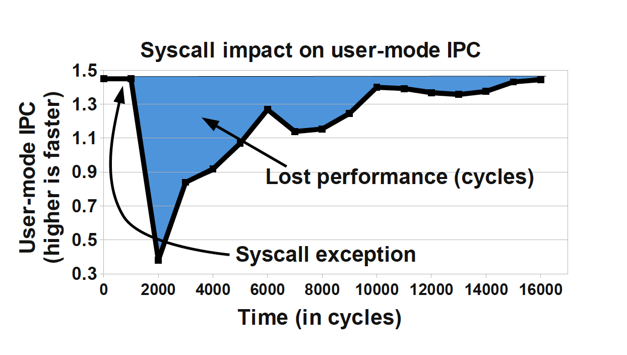
Figure 3-7. Impact of a system call (Soares and Stumm, 2010)
To mitigate this when possible, Linux provides a mechanism known as the vDSO (virtual dynamically shared object). This is a memory area in user space that is used to speed up syscalls that do not really require kernel privileges. It achieves this speed increase by not actually performing a context switch into kernel mode. Let’s look at an example to see how this works with a real syscall.
A very common Unix system call is gettimeofday(). This returns the “wallclock
time” as understood by the operating system. Behind the scenes, it is actually
just reading a kernel data structure to obtain the system clock time. As this is
side-effect-free, it does not actually need privileged access.
If we can use the vDSO to arrange for this data structure to be mapped into the address space of the user process, then there’s no need to perform the switch to kernel mode. As a result, the refill penalty shown in Figure 3-7 does not have to be paid.
Given how often most Java applications need to access timing data, this is a welcome performance boost. The vDSO mechanism generalizes this example slightly and can be a useful technique, even if it is available only on Linux.
A Simple System Model
In this section we cover a simple model for describing basic sources of possible performance problems. The model is expressed in terms of operating system observables of fundamental subsystems and can be directly related back to the outputs of standard Unix command-line tools.
The model is based on a simple conception of a Java application running on a Unix or Unix-like operating system. Figure 3-8 shows the basic components of the model, which consist of:
-
The hardware and operating system the application runs on
-
The JVM (or container) the application runs in
-
The application code itself
-
Any external systems the application calls
-
The incoming request traffic that is hitting the application
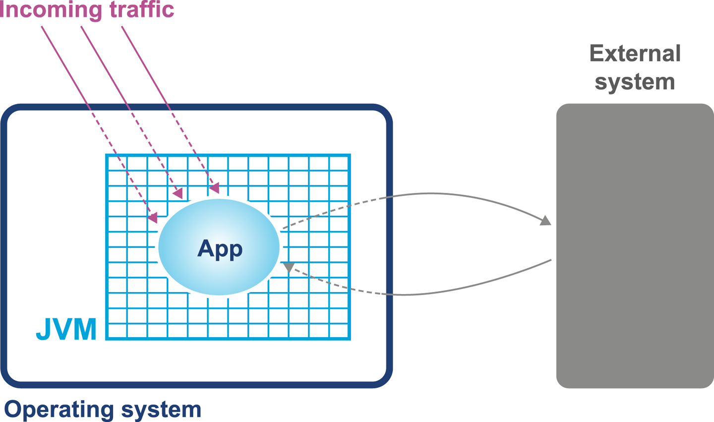
Figure 3-8. Simple system model
Any of these aspects of a system can be responsible for a performance problem. There are some simple diagnostic techniques that can be used to narrow down or isolate particular parts of the system as potential culprits for performance problems, as we will see in the next section.
Basic Detection Strategies
One definition for a well-performing application is that efficient use is being made of system resources. This includes CPU usage, memory, and network or I/O bandwidth.
Tip
If an application is causing one or more resource limits to be hit, then the result will be a performance problem.
The first step in any performance diagnosis is to recognize which resource limit is being hit. We cannot tune the appropriate performance metrics without dealing with the resource shortage—by increasing either the available resources or the efficiency of use.
It is also worth noting that the operating system itself should not normally be a major contributing factor to system utilization. The role of an operating system is to manage resources on behalf of user processes, not to consume them itself. The only real exception to this rule is when resources are so scarce that the OS is having difficulty allocating anywhere near enough to satisfy user requirements. For most modern server-class hardware, the only time this should occur is when I/O (or occasionally memory) requirements greatly exceed capability.
Utilizing the CPU
A key metric for application performance is CPU utilization. CPU cycles are quite often the most critical resource needed by an application, and so efficient use of them is essential for good performance. Applications should be aiming for as close to 100% usage as possible during periods of high load.
Tip
When you are analyzing application performance, the system must be under enough load to exercise it. The behavior of an idle application is usually meaningless for performance work.
Two basic tools that every performance engineer should be aware of are
vmstat and iostat.
On Linux and other Unixes, these command-line tools provide immediate and often very useful insight into the current state of the virtual memory and I/O subsystems, respectively.
The tools only provide numbers at the level of the entire host, but this is frequently enough to point the way to more detailed diagnostic approaches. Let’s take a look at how to use vmstat as an example:
$ vmstat 1
 r  b swpd  free    buff  cache   si   so  bi  bo   in   cs us sy  id wa st
 2  0   0 759860 248412 2572248    0    0   0  80   63  127  8  0  92  0  0
 2  0   0 759002 248412 2572248    0    0   0   0   55  103 12  0  88  0  0
 1  0   0 758854 248412 2572248    0    0   0  80   57  116  5  1  94  0  0
 3  0   0 758604 248412 2572248    0    0   0  14   65  142 10  0  90  0  0
 2  0   0 758932 248412 2572248    0    0   0  96   52  100  8  0  92  0  0
 2  0   0 759860 248412 2572248    0    0   0   0   60  112  3  0  97  0  0
The parameter 1 following vmstat indicates that we want vmstat to provide ongoing output (until interrupted via Ctrl-C) rather than a single snapshot.
New output lines are printed every second, which enables a performance engineer to leave this output running (or capture it into a log) while an initial performance test is performed.
The output of vmstat is relatively easy to understand and contains a large amount of useful information, divided into sections:
-
The first two columns show the number of runnable (
r) and blocked (b) processes. -
In the memory section, the amount of swapped and free memory is shown, followed by the memory used as buffer and as cache.
-
The swap section shows the memory swapped in from and out to disk (
siandso). Modern server-class machines should not normally experience very much swap activity. -
The block in and block out counts (
biandbo) show the number of 512-byte blocks that have been received from and sent to a block (I/O) device. -
In the system section, the number of interrupts (
in) and the number of context switches per second (cs) are displayed. -
The CPU section contains a number of directly relevant metrics, expressed as percentages of CPU time. In order, they are user time (
us), kernel time (sy, for “system time”), idle time (id), waiting time (wa), and “stolen time” (st, for virtual machines).
Over the course of the remainder of this book, we will meet many other, more sophisticated tools. However, it is important not to neglect the basic tools at our disposal. Complex tools often have behaviors that can mislead us, whereas the simple tools that operate close to processes and the operating system can convey clear and uncluttered views of how our systems are actually behaving.
Let’s consider an example. In “Context Switches” we discussed the impact of a context switch, and we saw the potential impact of a full context switch to kernel space in Figure 3-7. However, whether between user threads or into kernel space, context switches introduce unavoidable wastage of CPU resources.
A well-tuned program should be making maximum possible use of its resources, especially CPU. For workloads that are primarily dependent on computation (“CPU-bound” problems), the aim is to achieve close to 100% utilization of CPU for userland work.
To put it another way, if we observe that the CPU utilization is not approaching 100% user time, then the next obvious question is, “Why not?” What is causing the program to fail to achieve that? Are involuntary context switches caused by locks the problem? Is it due to blocking caused by I/O contention?
The vmstat tool can, on most operating systems (especially Linux), show the number
of context switches occurring, so a vmstat 1 run allows the analyst to
see the real-time effect of context switching. A process that is failing to achieve
100% userland CPU usage and is also displaying a high context switch rate is likely
to be either blocked on I/O or experiencing thread lock contention.
However, vmstat output is not enough to fully disambiguate these cases on its own. vmstat can help analysts detect I/O
problems, as it provides a crude view of I/O operations, but to detect thread lock contention in real time, tools like
VisualVM that can show the states of threads in a running process should be used.
An additional common tool is the statistical thread profiler that samples stacks
to provide a view of blocking code.
Garbage Collection
As we will see in Chapter 6, in the HotSpot JVM (by far
the most commonly used JVM) memory is allocated at startup and managed from
within user space. That means that system calls (such as sbrk()) are not
needed to allocate memory. In turn, this means that kernel-switching activity
for garbage collection is quite minimal.
Thus, if a system is exhibiting high levels of system CPU usage, then it is definitely not spending a significant amount of its time in GC, as GC activity burns user space CPU cycles and does not impact kernel space utilization.
On the other hand, if a JVM process is using 100% (or close to that) of CPU in user space,
then garbage collection is often the culprit. When analyzing a performance problem,
if simple tools (such as vmstat) show consistent 100% CPU usage, but with almost all
cycles being consumed by user space, then we should ask,
“Is it the JVM or user code that is responsible for this utilization?” In almost all
cases, high user space utilization by the JVM is caused by the GC subsystem, so a
useful rule of thumb is to check the GC log and see how often new entries are being
added to it.
Garbage collection logging in the JVM is incredibly cheap, to the point that even the most accurate measurements of the overall cost cannot reliably distinguish it from random background noise. GC logging is also incredibly useful as a source of data for analytics. It is therefore imperative that GC logs be enabled for all JVM processes, especially in production.
We will have a great deal to say about GC and the resulting logs later in the book. However, at this point, we would encourage the reader to consult with their operations staff and confirm whether GC logging is on in production. If not, then one of the key points of Chapter 7 is to build a strategy to enable this.
I/O
File I/O has traditionally been one of the murkier aspects of overall system performance. Partly this comes from its closer relationship with messy physical hardware, with engineers making quips about “spinning rust” and similar, but it is also because I/O lacks abstractions as clean as we see elsewhere in operating systems.
In the case of memory, the elegance of virtual memory as a separation mechanism works well. However, I/O has no comparable abstraction that provides suitable isolation for the application developer.
Fortunately, while most Java programs involve some simple I/O, the class of applications that make heavy use of the I/O subsystems is relatively small, and in particular, most applications do not simultaneously try to saturate I/O at the same time as either CPU or memory.
Not only that, but established operational practice has led to a culture in which production engineers are already aware of the limitations of I/O, and actively monitor processes for heavy I/O usage.
For the performance analyst/engineer, it suffices to have an awareness of the I/O
behavior of our applications. Tools such as iostat (and even vmstat) have the
basic counters (e.g., blocks in or out), which are often all we need for basic diagnosis,
especially if we make the assumption that only one I/O-intensive application is
present per host.
Finally, it’s worth mentioning one aspect of I/O that is becoming more widely used across a class of Java applications that have a dependency on I/O but also stringent performance applications.
Kernel bypass I/O
For some high-performance applications, the cost of using the kernel to copy data from, for example, a buffer on a network card and place it into a user space region is prohibitively high. Instead, specialized hardware and software is used to map data directly from a network card into a user-accessible area. This approach avoids a “double copy” as well as crossing the boundary between user space and kernel, as we can see in Figure 3-9.
However, Java does not provide specific support for this model, and instead applications that wish to make use of it rely upon custom (native) libraries to implement the required semantics. It can be a very useful pattern and is increasingly commonly implemented in systems that require very high-performance I/O.
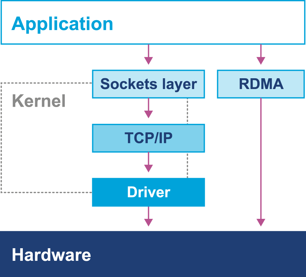
Figure 3-9. Kernel bypass I/O
Note
In some ways, this is reminiscent of Java’s New I/O (NIO) API that was introduced to allow Java I/O to bypass the Java heap and work directly with native memory and underlying I/O.
In this chapter so far we have discussed operating systems running on top of “bare metal.” However, increasingly, systems run in virtualized environments, so to conclude this chapter, let’s take a brief look at how virtualization can fundamentally change our view of Java application performance.
Mechanical Sympathy
Mechanical sympathy is the idea that having an appreciation of the hardware is invaluable for those cases where we need to squeeze out extra performance.
You don’t have to be an engineer to be a racing driver, but you do have to have mechanical sympathy.
Jackie Stewart
The phrase was originally coined by Martin Thompson, as a direct reference to Jackie Stewart and his car. However, as well as the extreme cases, it is also useful to have a baseline understanding of the concerns outlined in this chapter when dealing with production problems and looking at improving the overall performance of your application.
For many Java developers, mechanical sympathy is a concern that it is possible to ignore. This is because the JVM provides a level of abstraction away from the hardware to unburden the developer from a wide range of performance concerns. Developers can use Java and the JVM quite successfully in the high-performance and low-latency space, by gaining an understanding of the JVM and the interaction it has with hardware. One important point to note is that the JVM actually makes reasoning about performance and mechanical sympathy harder, as there is more to consider. In Chapter 14 we will describe how high-performance logging and messaging systems work and how mechanical sympathy is appreciated.
Let’s look at an example: the behavior of cache lines.
In this chapter we have discussed the benefit of processor caching. The use of cache lines enables the fetching of blocks of memory. In a multithreaded environment cache lines can cause a problem when you have two threads attempting to read or write to a variable located on the same cache line.
A race essentially occurs where two threads now attempt to modify the same cache line. The first one will invalidate the cache line on the second thread, causing it to be reread from memory. Once the second thread has performed the operation, it will then invalidate the cache line in the first. This ping-pong behavior results in a drop-off in performance known as false sharing—but how can this be fixed?
Mechanical sympathy would suggest that first we need to understand that this is happening and only after that determine how to resolve it. In Java the layout of fields in an object is not guaranteed, meaning it is easy to find variables sharing a cache line. One way to get around this would be to add padding around the variables to force them onto a different cache line. “Queues” will demonstrate one way we can achieve this using a low-level queue in the Agrona project.
Virtualization
Virtualization comes in many forms, but one of the most common is to run a copy of an operating system as a single process on top of an already running OS. This leads to the situation represented in Figure 3-10, where the virtual environment runs as a process inside the unvirtualized (or “real”) operating system that is executing on bare metal.
A full discussion of virtualization, the relevant theory, and its implications for application performance tuning would take us too far afield. However, some mention of the differences that virtualization causes seems appropriate, especially given the increasing amount of applications running in virtual, or cloud, environments.
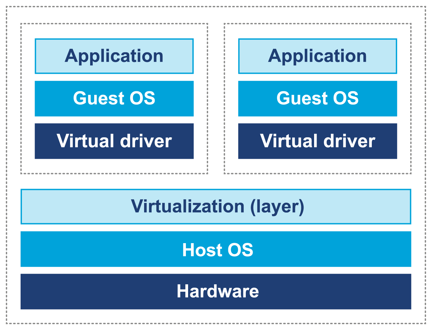
Figure 3-10. Virtualization of operating systems
Although virtualization was originally developed in IBM mainframe environments as early as the 1970s, it was not until recently that x86 architectures were capable of supporting “true” virtualization. This is usually characterized by these three conditions:
-
Programs running on a virtualized OS should behave essentially the same as when running on bare metal (i.e., unvirtualized).
-
The hypervisor must mediate all access to hardware resources.
-
The overhead of the virtualization must be as small as possible, and not a significant fraction of execution time.
In a normal, unvirtualized system, the OS kernel runs in a special, privileged mode (hence the need to switch into kernel mode). This gives the OS direct access to hardware. However, in a virtualized system, direct access to hardware by a guest OS is prohibited.
One common approach is to rewrite the privileged instructions in terms of unprivileged instructions. In addition, some of the OS kernel’s data structures need to be “shadowed” to prevent excessive cache flushing (e.g., of TLBs) during context switches.
Some modern Intel-compatible CPUs have hardware features designed to improve the performance of virtualized OSs. However, it is apparent that even with hardware assists, running inside a virtual environment presents an additional level of complexity for performance analysis and tuning.
The JVM and the Operating System
The JVM provides a portable execution environment that is independent of the operating system, by providing a common interface to Java code. However, for some fundamental services, such as thread scheduling (or even something as mundane as getting the time from the system clock), the underlying operating system must be accessed.
This capability is provided by native methods, which are denoted by the keyword native. They are written in C, but are accessible as ordinary Java methods. This interface is referred to as the Java Native Interface (JNI). For example, java.lang.Object declares these nonprivate native methods:
publicfinalnativeClass<?>getClass();publicnativeinthashCode();protectednativeObjectclone()throwsCloneNotSupportedException;publicfinalnativevoidnotify();publicfinalnativevoidnotifyAll();publicfinalnativevoidwait(longtimeout)throwsInterruptedException;
As all these methods deal with relatively low-level platform concerns, let’s look at a more straightforward and familiar example: getting the system time.
Consider the os::javaTimeMillis() function. This is the (system-specific) code responsible for implementing the Java System.currentTimeMillis() static method. The code that does the actual work is implemented in C++, but is accessed from Java via a “bridge” of C code. Let’s look at how this code is actually called in HotSpot.
As you can see in Figure 3-11, the native System.currentTimeMillis() method is mapped to the JVM entry point method JVM_CurrentTimeMillis().
This mapping is achieved via the JNI Java_java_lang_System_registerNatives() mechanism contained in java/lang/System.c.
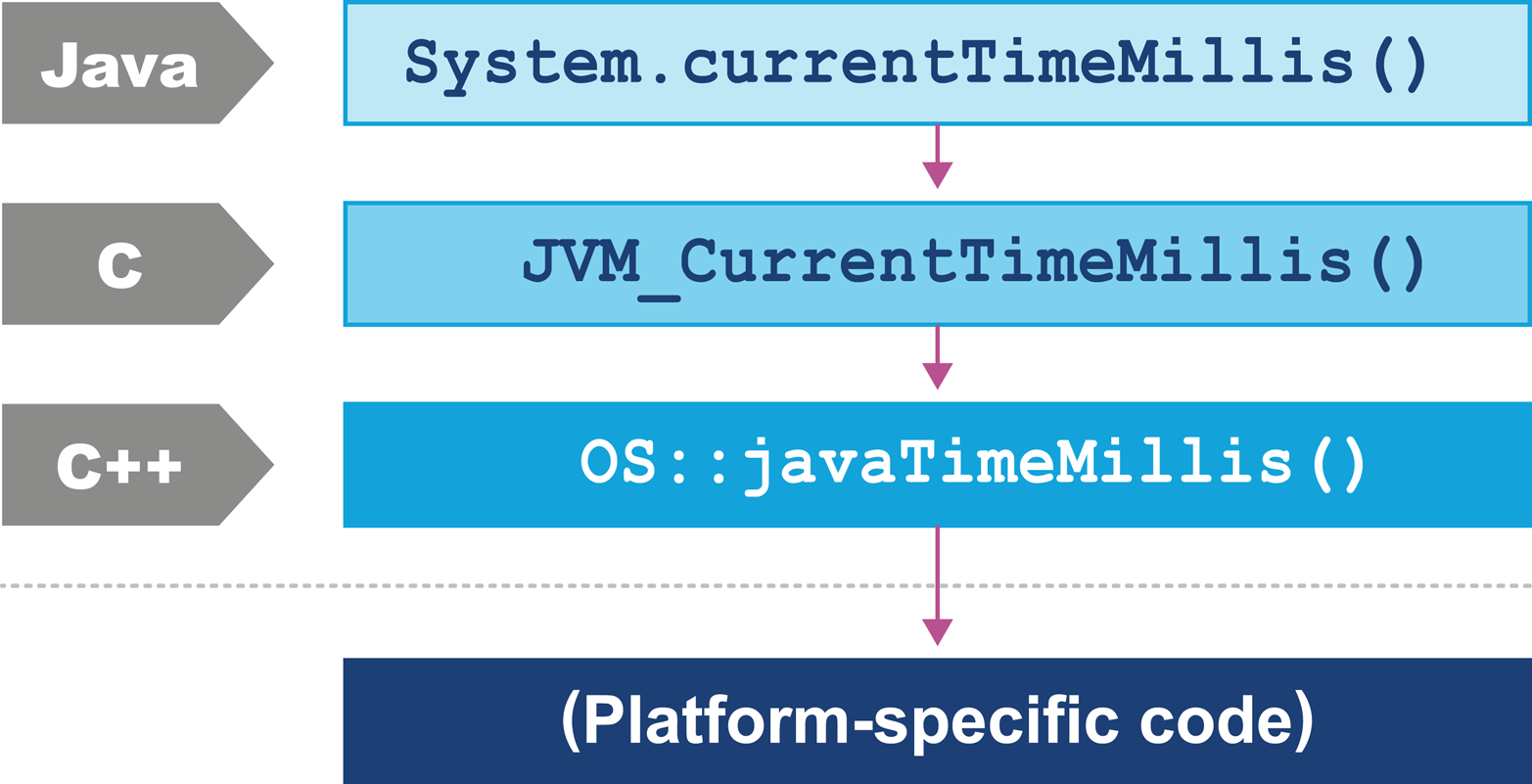
Figure 3-11. The HotSpot calling stack
JVM_CurrentTimeMillis() is a call to the VM entry point method.
This presents as a C function but is really a C++ function exported with a C calling convention.
The call boils down to the call os::javaTimeMillis() wrapped in a couple of OpenJDK macros.
This method is defined in the os namespace, and is unsurprisingly operating system–dependent. Definitions for this method are provided by the OS-specific subdirectories of source code within OpenJDK. This provides a simple demonstration of how the platform-independent parts of Java can call into services that are provided by the underlying operating system and hardware.
Summary
Processor design and modern hardware have changed enormously over the last 20 years. Driven by Moore’s Law and by engineering limitations (notably the relatively slow speed of memory), advances in processor design have become somewhat esoteric. The cache miss rate has become the most obvious leading indicator of how performant an application is.
In the Java space, the design of the JVM allows it to make use of additional processor cores even for single-threaded application code. This means that Java applications have received significant performance advantages from hardware trends, compared to other environments.
As Moore’s Law fades, attention will turn once again to the relative performance of software. Performance-minded engineers need to understand at least the basic points of modern hardware and operating systems to ensure that they can make the most of their hardware and not fight against it.
In the next chapter we will introduce the core methodology of performance tests. We will discuss the primary types of performance tests, the tasks that need to be undertaken, and the overall lifecycle of performance work. We will also catalogue some common best practices (and antipatterns) in the performance space.
1 John L. Hennessy and David A. Patterson, From Computer Architecture: A Quantitative Approach, 5th ed. (Burlington, MA: Morgan Kaufmann, 2011).
2 Access times shown in terms of number of clock cycles per operation; data provided by Google.
3 Livio Stoares and Michael Stumm, “FlexSC: Flexible System Call Scheduling with Exception-Less System Calls,” in OSDI’10, Proceedings of the 9th USENIX Conference on Operating Systems Design and Implementation (Berkeley, CA: USENIX Association, 2010), 33–46.