Table of Contents for
Optimizing Java
 Optimizing Java
Published by
O'Reilly Media, Inc., 2018
Optimizing Java
Published by
O'Reilly Media, Inc., 2018
- nav
- Cover
- Optimizing Java
- Optimizing Java
- Dedication
- Foreword
- Preface
- 1. Optimization and Performance Defined
- 2. Overview of the JVM
- 3. Hardware and Operating Systems
- 4. Performance Testing Patterns and Antipatterns
- 5. Microbenchmarking and Statistics
- 6. Understanding Garbage Collection
- 7. Advanced Garbage Collection
- 8. GC Logging, Monitoring, Tuning, and Tools
- 9. Code Execution on the JVM
- 10. Understanding JIT Compilation
- 11. Java Language Performance Techniques
- 12. Concurrent Performance Techniques
- 13. Profiling
- 14. High-Performance Logging and Messaging
- 15. Java 9 and the Future
- Index
- About the Authors
- Colophon
Chapter 6. Understanding Garbage Collection
The Java environment has several iconic or defining features, and garbage collection is one of the most immediately recognizable. However, when the platform was first released, there was considerable hostility to GC. This was fueled by the fact that Java deliberately provided no language-level way to control the behavior of the collector (and continues not to, even in modern versions).1
This meant that in the early days, there was a certain amount of frustration over the performance of Java’s GC, and this fed into perceptions of the platform as a whole.
However, the early vision of mandatory, non-user-controllable GC has been more than vindicated, and these days very few application developers would attempt to defend the opinion that memory should be managed by hand. Even modern takes on systems programming languages (e.g., Go and Rust) regard memory management as the proper domain of the compiler and runtime rather than the programmer (in anything other than exceptional circumstances).
The essence of Java’s garbage collection is that rather than requiring the programmer to understand the precise lifetime of every object in the system, the runtime should keep track of objects on the programmer’s behalf and automatically get rid of objects that are no longer required. The automatically reclaimed memory can then be wiped and reused.
There are two fundamental rules of garbage collection that all implementations are subject to:
-
Algorithms must collect all garbage.
-
No live object must ever be collected.
Of these two rules, the second is by far the most important. Collecting a live object could lead to segmentation faults or (even worse) silent corruption of program data. Java’s GC algorithms need to be sure that they will never collect an object the program is still using.
The idea of the programmer surrendering some low-level control in exchange for not having to account for every low-level detail by hand is the essence of Java’s managed approach and expresses James Gosling’s conception of Java as a blue-collar language for getting things done.
In this chapter, we will meet some of the basic theory that underpins Java garbage collection, and explain why it is one of the hardest parts of the platform to fully understand and to control. We will also introduce the basic features of HotSpot’s runtime system, including such details as how HotSpot represents objects in the heap at runtime.
Toward the end of the chapter, we will introduce the simplest of HotSpot’s production collectors, the parallel collectors, and explain some of the details that make them so useful for many workloads.
Introducing Mark and Sweep
Most Java programmers, if pressed, can recall that Java’s GC relies on an algorithm called mark and sweep, but most also struggle to recall any details as to how the process actually operates.
In this section we will introduce a basic form of the algorithm and show how it can be used to reclaim memory automatically. This is a deliberately simplified form of the algorithm and is only intended to introduce a few basic concepts—it is not representative of how production JVMs actually carry out GC.
This introductory form of the mark-and-sweep algorithm uses an allocated object list to hold a pointer to each object that has been allocated, but not yet reclaimed. The overall GC algorithm can then be expressed as:
-
Loop through the allocated list, clearing the mark bit.
-
Starting from the GC roots, find the live objects.
-
Set a mark bit on each object reached.
-
Loop through the allocated list, and for each object whose mark bit hasn’t been set:
-
Reclaim the memory in the heap and place it back on the free list.
-
Remove the object from the allocated list.
-
The live objects are usually located depth-first, and the resulting graph of objects is called the live object graph. It is sometimes also called the transitive closure of reachable objects, and an example can be seen in Figure 6-1.
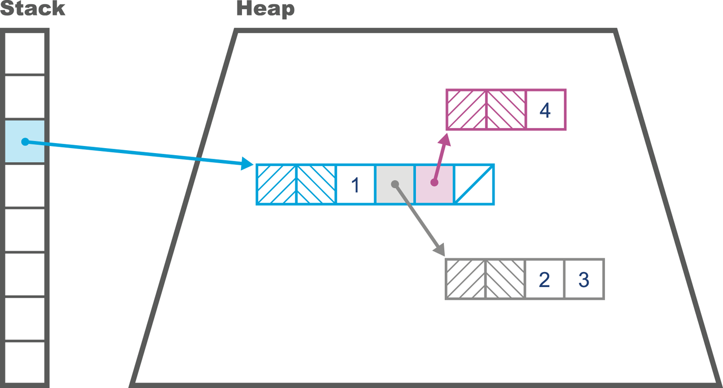
Figure 6-1. Simple view of memory layout
The state of the heap can be hard to visualize, but fortunately there are some simple tools to help us. One of the simplest is the jmap -histo command-line tool. This shows the number of bytes allocated per type, and the number of instances that are collectively responsible for that memory usage. It produces output like the following:
num    #instances       #bytes  class name
----------------------------------------------
  1:        20839     14983608  [B
  2:       118743     12370760  [C
  3:        14528      9385360  [I
  4:          282      6461584  [D
  5:       115231      3687392  java.util.HashMap$Node
  6:       102237      2453688  java.lang.String
  7:        68388      2188416  java.util.Hashtable$Entry
  8:         8708      1764328  [Ljava.util.HashMap$Node;
  9:        39047      1561880  jdk.nashorn.internal.runtime.CompiledFunction
 10:        23688      1516032  com.mysql.jdbc.Co...$BooleanConnectionProperty
 11:        24217      1356152  jdk.nashorn.internal.runtime.ScriptFunction
 12:        27344      1301896  [Ljava.lang.Object;
 13:        10040      1107896  java.lang.Class
 14:        44090      1058160  java.util.LinkedList$Node
 15:        29375       940000  java.util.LinkedList
 16:        25944       830208  jdk.nashorn.interna...FinalScriptFunctionData
 17:           20       655680  [Lscala.concurrent.forkjoin.ForkJoinTask;
 18:        19943       638176  java.util.concurrent.ConcurrentHashMap$Node
 19:          730       614744  [Ljava.util.Hashtable$Entry;
 20:        24022       578560  [Ljava.lang.Class;
There is also a GUI tool available: the Sampling tab of VisualVM, introduced in Chapter 2. The VisualGC plug-in to VisualVM provides a real-time view of how the heap is changing, but in general the moment-to-moment view of the heap is not sufficient for accurate analysis and instead we should use GC logs for better insight—this will be a major theme of Chapter 8.
Garbage Collection Glossary
The jargon used to describe GC algorithms is sometimes a bit confusing (and the meaning of some of the terms has changed over time). For the sake of clarity, we include a basic glossary of how we use specific terms:
- Stop-the-world (STW)
-
The GC cycle requires all application threads to be paused while garbage is collected. This prevents application code from invalidating the GC thread’s view of the state of the heap. This is the usual case for most simple GC algorithms.
- Concurrent
-
GC threads can run while application threads are running. This is very, very difficult to achieve, and very expensive in terms of computation expended. Virtually no algorithms are truly concurrent. Instead, complex tricks are used to give most of the benefits of concurrent collection. In “CMS” we’ll meet HotSpot’s Concurrent Mark and Sweep (CMS) collector, which, despite its name, is perhaps best described as a “mostly concurrent” collector.
- Parallel
- Exact
-
An exact GC scheme has enough type information about the state of the heap to ensure that all garbage can be collected on a single cycle. More loosely, an exact scheme has the property that it can always tell the difference between an
intand a pointer. - Conservative
-
A conservative scheme lacks the information of an exact scheme. As a result, conservative schemes frequently fritter away resources and are typically far less efficient due to their fundamental ignorance of the type system they purport to represent.
- Moving
-
In a moving collector, objects can be relocated in memory. This means that they do not have stable addresses. Environments that provide access to raw pointers (e.g., C++) are not a natural fit for moving collectors.
- Compacting
-
At the end of the collection cycle, allocated memory (i.e., surviving objects) is arranged as a single contiguous region (usually at the start of the region), and there is a pointer indicating the start of empty space that is available for objects to be written into. A compacting collector will avoid memory fragmentation.
- Evacuating
-
At the end of the collection cycle, the collected region is totally empty, and all live objects have been moved (evacuated) to another region of memory.
In most other languages and environments, the same terms are used. For example, the JavaScript runtime of the Firefox web browser (SpiderMonkey) also makes use of garbage collection, and in recent years has been adding features (e.g., exactness and compaction) that are already present in GC implementations in Java.
Introducing the HotSpot Runtime
In addition to the general GC terminology, HotSpot introduces terms that are more specific to the implementation. To obtain a full understanding of how garbage collection works on this JVM, we need to get to grips with some of the details of HotSpot’s internals.
For what follows it will be very helpful to remember that Java has only two sorts of value:
-
Primitive types (
byte,int, etc.) -
Object references
Many Java programmers loosely talk about objects, but for our purposes it is important to remember that, unlike C++, Java has no general address dereference mechanism and can only use an offset operator (the . operator) to access fields and call methods on object references. Also keep in mind that Java’s method call semantics are purely call-by-value, although for object references this means that the value that is copied is the address of the object in the heap.
Representing Objects at Runtime
HotSpot represents Java objects at runtime via a structure called an oop. This is short for ordinary object pointer, and is a genuine pointer in the C sense. These pointers can be placed in local variables of reference type where they point from the stack frame of the Java method into the memory area comprising the Java heap.
There are several different data structures that comprise the family of oops, and the sort that represent instances of a Java class are called instanceOops.
The memory layout of an instanceOop starts with two machine words of header present on every object. The mark word is the first of these, and is a pointer that points at instance-specific metadata. Next is the klass word, which points at class-wide metadata.
In Java 7 and before, the klass word of an instanceOop points into an area of memory called PermGen, which was a part of the Java heap. The general rule is that anything in the Java heap must have an object header. In these older versions of Java we refer to the metadata as a klassOop. The memory layout of a klassOop is simple—it’s just the object header immediately followed by the klass metadata.
From Java 8 onward, the klasses are held outside of the main part of the Java heap (but not outside the C heap of the JVM process). Klass words in these versions of Java do not require an object header, as they point outside the Java heap.
Note
The k at the start is used to help disambiguate the klassOop from an instanceOop representing the Java Class<?> object; they are not the same thing.
In Figure 6-2 we can see the difference: fundamentally the klassOop contains the virtual function table (vtable) for the class, whereas the Class object contains an array of references to Method objects for use in reflective invocation. We will have more to say on this subject in Chapter 9 when we discuss JIT compilation.
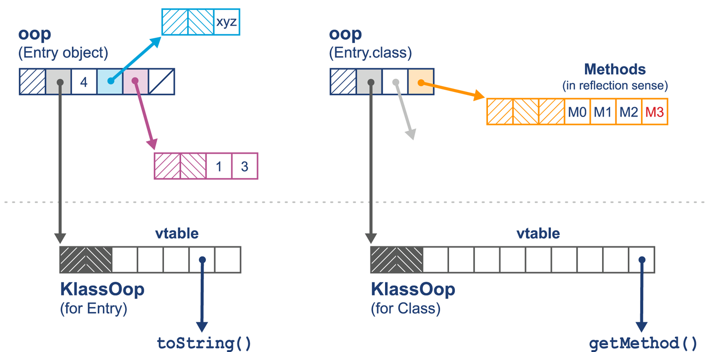
Figure 6-2. klassOops and Class objects
Oops are usually machine words, so 32 bits on a legacy 32-bit machine, and 64 bits on a modern processor. However, this has the potential to waste a possibly significant amount of memory. To help mitigate this, HotSpot provides a technique called compressed oops. If the option:
-XX:+UseCompressedOops
is set (and it is the default for 64-bit heaps from Java 7 and upward), then the following oops in the heap will be compressed:
-
The klass word of every object in the heap
-
Instance fields of reference type
-
Every element of an array of objects
This means that, in general, a HotSpot object header consists of:
-
Mark word at full native size
-
Klass word (possibly compressed)
-
Length word if the object is an array—always 32 bits
-
A 32-bit gap (if required by alignment rules)
The instance fields of the object then follow immediately after the header. For klassOops, the vtable of methods follows directly after the klass word. The memory layout for compressed oops can be seen in Figure 6-3.
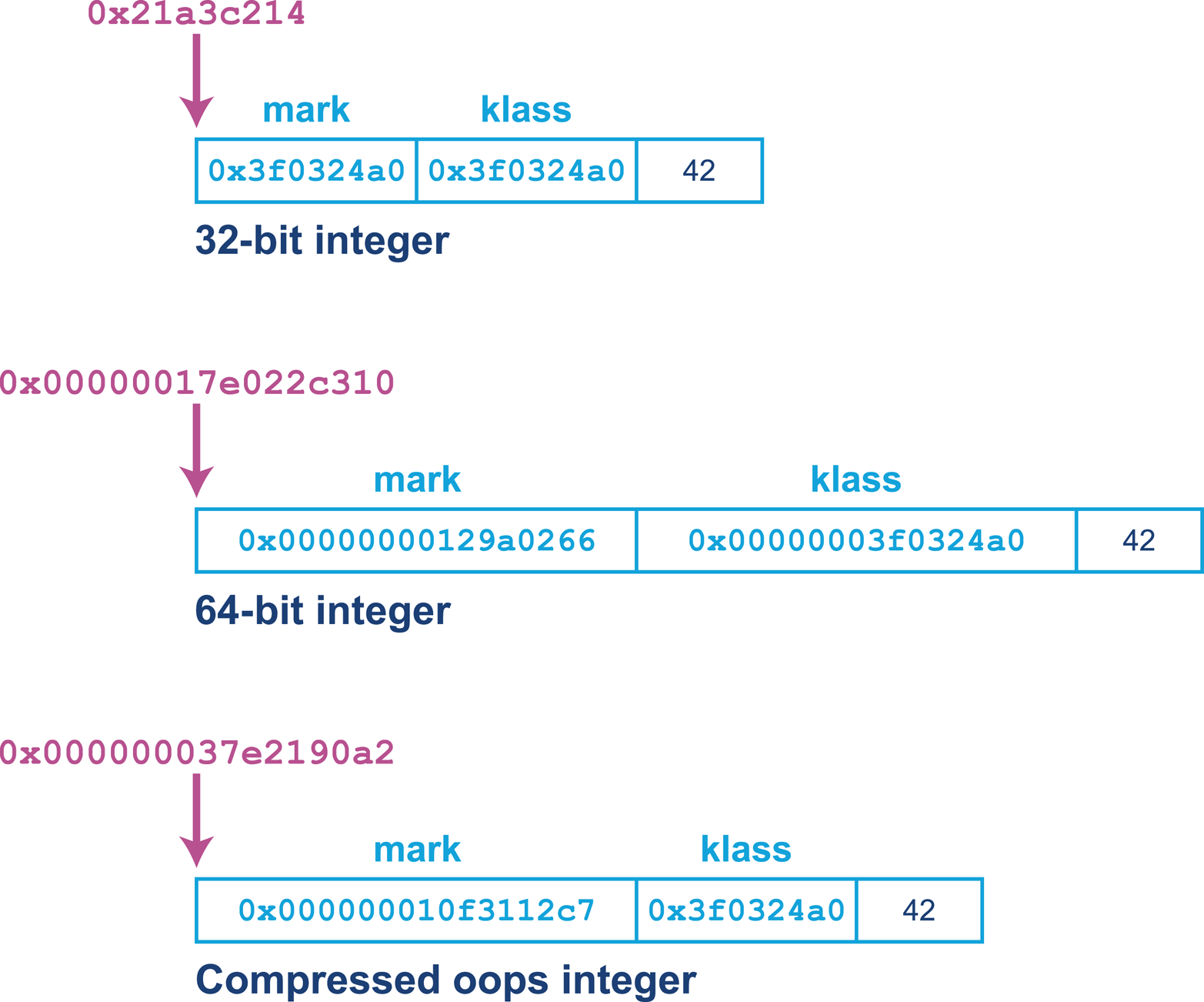
Figure 6-3. Compressed oops
In the past, some extremely latency-sensitive applications could occasionally see improvements by switching off the compressed oops feature—at the cost of increased heap size (typically an increase of 10–50%). However, the class of applications for which this would yield measurable performance benefits is very small, and for most modern applications this would be a classic example of the Fiddling with Switches antipattern we saw in Chapter 4.
As we remember from basic Java, arrays are objects. This means that the JVM’s arrays are represented as oops as well. This is why arrays have a third word of metadata as well as the usual mark and klass words. This third word is the array’s length—which also explains why array indices in Java are limited to 32-bit values.
Note
The use of additional metadata to carry an array’s length alleviates a whole class of problems present in C and C++ where not knowing the length of the array means that additional parameters must be passed to functions.
The managed environment of the JVM does not allow a Java reference to point anywhere but at an instanceOop (or null). This means that at a low level:
-
A Java value is a bit pattern corresponding either to a primitive value or to the address of an instanceOop (a reference).
-
Any Java reference considered as a pointer refers to an address in the main part of the Java heap.
-
Addresses that are the targets of Java references contain a mark word followed by a klass word as the next machine word.
-
A klassOop and an instance of
Class<?>are different (as the former lives in the metadata area of the heap), and a klassOop cannot be placed into a Java variable.
HotSpot defines a hierarchy of oops in .hpp files that are kept in hotspot/src/share/vm/oops in the OpenJDK 8 source tree. The overall inheritance hierarchy for oops looks like this:
oop (abstract base)
 instanceOop (instance objects)
 methodOop (representations of methods)
 arrayOop (array abstract base)
 symbolOop (internal symbol / string class)
 klassOop (klass header) (Java 7 and before only)
 markOop
This use of oop structures to represent objects at runtime, with one pointer to house class-level metadata and another to house instance metadata, is not particularly unusual. Many other JVMs and other execution environments use a related mechanism. For example, Apple’s iOS uses a similar scheme for representing objects.
GC Roots and Arenas
Articles and blog posts about HotSpot frequently refer to GC roots. These are “anchor points” for memory, essentially known pointers that originate from outside a memory pool of interest and point into it. They are external pointers as opposed to internal pointers, which originate inside the memory pool and point to another memory location within the memory pool.
We saw an example of a GC root in Figure 6-1. However, as we will see, there are other sorts of GC root, including:
-
Stack frames
-
JNI
-
Registers (for the hoisted variable case)
-
Code roots (from the JVM code cache)
-
Globals
-
Class metadata from loaded classes
If this definition seems rather complex, then the simplest example of a GC root is a local variable of reference type that will always point to an object in the heap (provided it is not null).
The HotSpot garbage collector works in terms of areas of memory called arenas. This is a very low-level mechanism, and Java developers usually don’t need to consider the operation of the memory system in such detail. However, performance specialists sometimes need to delve deeper into the internals of the JVM, and so a familiarity with the concepts and terms used in the literature is helpful.
One important fact to remember is that HotSpot does not use system calls to manage the Java heap. Instead, as we discussed in “Basic Detection Strategies”, HotSpot manages the heap size from user space code, so we can use simple observables to determine whether the GC subsystem is causing some types of performance problems.
In the next section, we’ll take a closer look at two of the most important characteristics that drive the garbage collection behavior of any Java or JVM workload. A good understanding of these characteristics is essential for any developer who wants to really grasp the factors that drive Java GC (which is one of the key overall drivers for Java performance).
Allocation and Lifetime
There are two primary drivers of the garbage collection behavior of a Java application:
-
Allocation rate
-
Object lifetime
The allocation rate is the amount of memory used by newly created objects over some time period (usually measured in MB/s). This is not directly recorded by the JVM, but is a relatively easy observable to estimate, and tools such as Censum can determine it precisely.
By contrast, the object lifetime is normally a lot harder to measure (or even estimate). In fact, one of the major arguments against using manual memory management is the complexity involved in truly understanding object lifetimes for a real application. As a result, object lifetime is if anything even more fundamental than allocation rate.
Note
Garbage collection can also be thought of as “memory reclamation and reuse.” The ability to use the same physical piece of memory over and over again, because objects are short-lived, is a key assumption of garbage collection techniques.
The idea that objects are created, they exist for a time, and then the memory used to store their state can be reclaimed is essential; without it, garbage collection would not work at all. As we will see in Chapter 7, there are a number of different tradeoffs that garbage collectors must balance—and some of the most important of these tradeoffs are driven by lifetime and allocation concerns.
Weak Generational Hypothesis
One key part of the JVM’s memory management relies upon an observed runtime effect of software systems, the Weak Generational Hypothesis:
The distribution of object lifetimes on the JVM and similar software systems is bimodal—with the vast majority of objects being very short-lived and a secondary population having a much longer life expectancy.
This hypothesis, which is really an experimentally observed rule of thumb about the behavior of object-oriented workloads, leads to an obvious conclusion: garbage-collected heaps should be structured in such a way as to allow short-lived objects to be easily and quickly collected, and ideally for long-lived objects to be separated from short-lived objects.
HotSpot uses several mechanisms to try to take advantage of the Weak Generational Hypothesis:
-
It tracks the “generational count” of each object (the number of garbage collections that the object has survived so far).
-
With the exception of large objects, it creates new objects in the “Eden” space (also called the “Nursery”) and expects to move surviving objects.
-
It maintains a separate area of memory (the “old” or “Tenured” generation) to hold objects that are deemed to have survived long enough that they are likely to be long-lived.
This approach leads to the view shown in simplified form in Figure 6-4, where objects that have survived a certain number of garbage collection cycles are promoted to the Tenured generation. Note the continuous nature of the regions, as shown in the diagram.
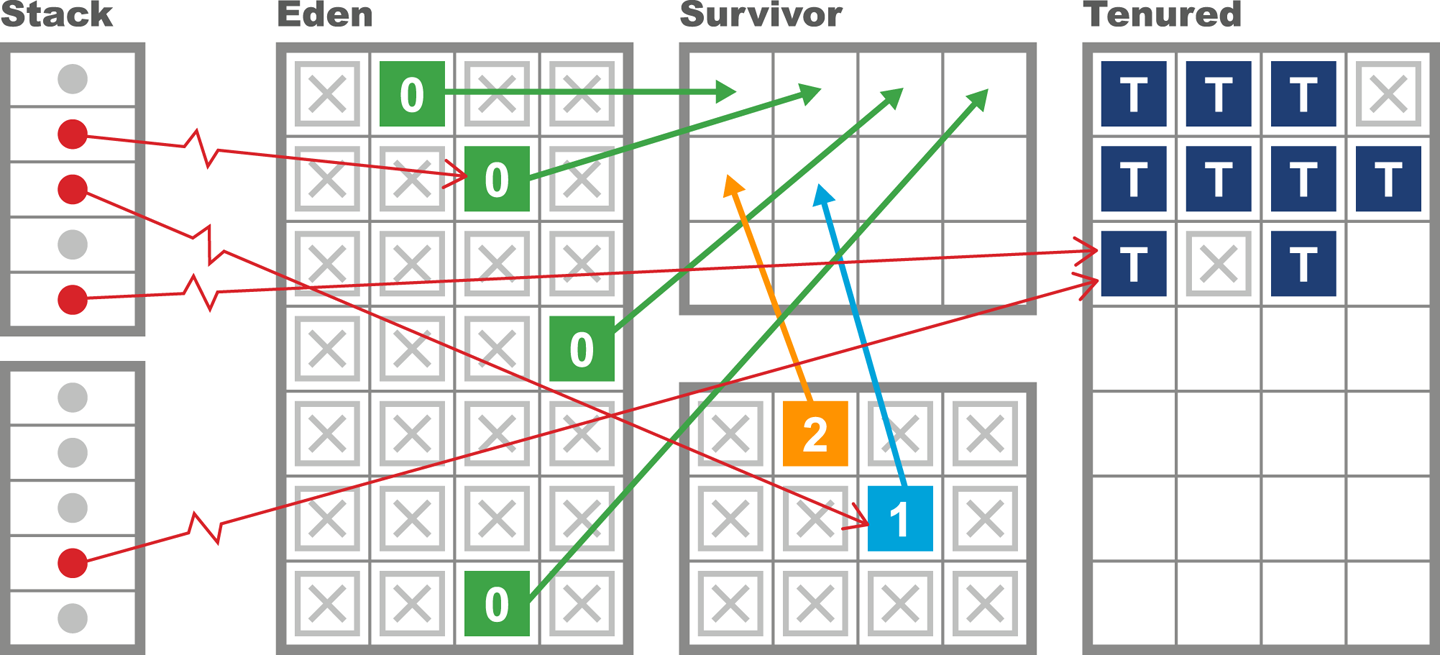
Figure 6-4. Generational collection
Dividing up memory into different regions for purposes of generational collection has some additional consequences in terms of how HotSpot implements a mark-and-sweep collection. One important technique involves keeping track of pointers that point into the young generation from outside. This saves the GC cycle from having to traverse the entire object graph in order to determine the young objects that are still live.
Note
“There are few references from old to young objects” is sometimes cited as a secondary part of the Weak Generational Hypothesis.
To facilitate this process, HotSpot maintains a structure called a card table to help record which old-generation objects could potentially point at young objects. The card table is essentially an array of bytes managed by the JVM. Each element of the array corresponds to a 512-byte area of old-generation space.
The central idea is that when a field of reference type on an old object o is modified, the card table entry for the card containing the instanceOop corresponding to o is marked as dirty. HotSpot achieves this with a simple write barrier when updating reference fields. It essentially boils down to this bit of code being executed after the field store:
cards[*instanceOop>>9]=0;
Note that the dirty value for the card is 0, and the right-shift by 9 bits gives the size of the card table as 512 bytes.
Finally, we should note that the description of the heap in terms of old and young areas is historically the way that Java’s collectors have managed memory. With the arrival of Java 8u40, a new collector (“Garbage First,” or G1) reached production quality. G1 has a somewhat different view of how to approach heap layout, as we will see in “CMS”. This new way of thinking about heap management will be increasingly important, as Oracle’s intention is for G1 to become the default collector from Java 9 onward.
Garbage Collection in HotSpot
Recall that unlike C/C++ and similar environments, Java does not use the operating system to manage dynamic memory. Instead, the JVM allocates (or reserves) memory up front, when the JVM process starts, and manages a single, contiguous memory pool from user space.
As we have seen, this pool of memory is made up of different regions with dedicated purposes, and the address that an object resides at will very often change over time as the collector relocates objects, which are normally created in Eden. Collectors that perform relocation are known as “evacuating” collectors, as mentioned in the “Garbage Collection Glossary”. Many of the collectors that HotSpot can use are evacuating.
Thread-Local Allocation
The JVM uses a performance enhancement to manage Eden. This is a critical region to manage efficiently, as it is where most objects are created, and very short-lived objects (those with lifetimes less than the remaining time to the next GC cycle) will never be located anywhere else.
For efficiency, the JVM partitions Eden into buffers and hands out individual regions of Eden for application threads to use as allocation regions for new objects. The advantage of this approach is that each thread knows that it does not have to consider the possibility that other threads are allocating within that buffer. These regions are called thread-local allocation buffers (TLABs).
Note
HotSpot dynamically sizes the TLABs that it gives to application threads, so if a thread is burning through memory it can be given larger TLABs to reduce the overhead in providing buffers to the thread.
The exclusive control that an application thread has over its TLABs means that allocation is O(1) for JVM threads. This is because when a thread creates a new object, storage is allocated for the object, and the thread-local pointer is updated to the next free memory address. In terms of the C runtime, this is a simple pointer bump—that is, one additional instruction to move the “next free” pointer onward.
This behavior can be seen in Figure 6-5, where each application thread holds a buffer to allocate new objects. If the application thread fills the buffer, then the JVM provides a pointer to a new area of Eden.
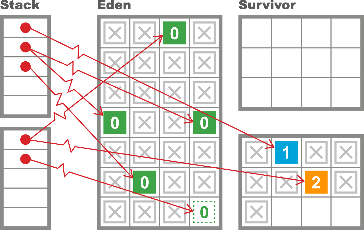
Figure 6-5. Thread-local allocation
Hemispheric Collection
One particular special case of the evacuating collector is worth noting. Sometimes referred to as a hemispheric evacuating collector, this type of collector uses two (usually equal-sized) spaces. The central idea is to use the spaces as a temporary holding area for objects that are not actually long-lived. This prevents short-lived objects from cluttering up the Tenured generation and reduces the frequency of full GCs. The spaces have a couple of basic properties:
-
When the collector is collecting the currently live hemisphere, objects are moved in a compacting fashion to the other hemisphere and the collected hemisphere is emptied for reuse.
-
One half of the space is kept completely empty at all times.
This approach does, of course, use twice as much memory as can actually be held within the hemispheric part of the collector. This is somewhat wasteful, but it is often a useful technique if the size of the spaces is not excessive. HotSpot uses this hemispheric approach in combination with the Eden space to provide a collector for the young generation.
The hemispheric part of HotSpot’s young heap is referred to as the survivor spaces. As we can see from the view of VisualGC shown in Figure 6-6, the survivor spaces are normally relatively small as compared to Eden, and the role of the survivor spaces swaps with each young generational collection. We will discuss how to tune the size of the survivor spaces in Chapter 8.
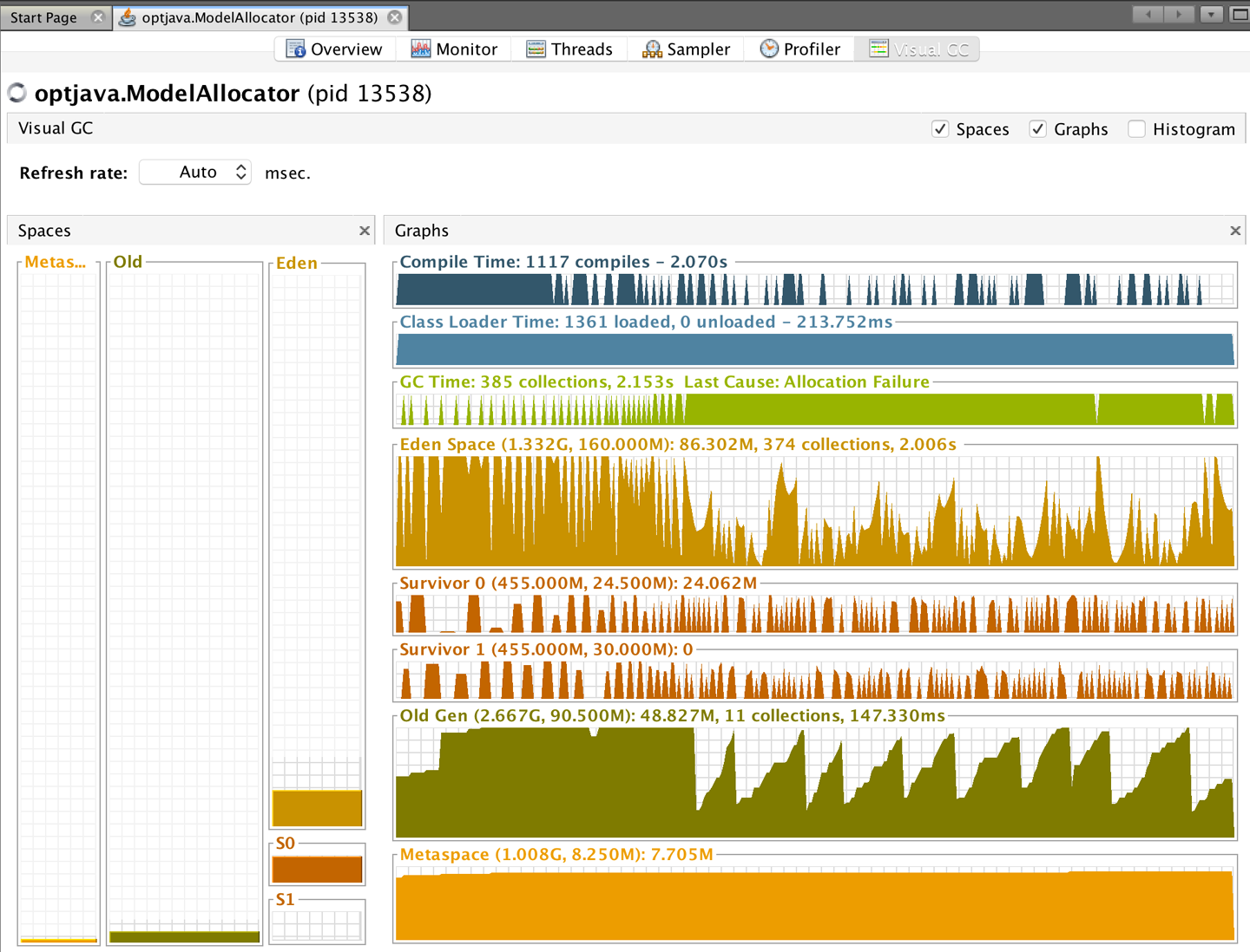
Figure 6-6. The VisualGC plug-in
The VisualGC plug-in for VisualVM, introduced in “VisualVM”, is a very useful initial GC debugging tool. As we will discuss in Chapter 7, the GC logs contain far more useful information and allow a much deeper analysis of GC than is possible from the moment-to-moment JMX data that VisualGC uses. However, when starting a new analysis, it is often helpful to simply eyeball the application’s memory usage.
Using VisualGC it is possible to see some aggregate effects of garbage collection, such as objects being relocated in the heap, and the cycling between survivor spaces that happens at each young collection.
The Parallel Collectors
In Java 8 and earlier versions, the default collectors for the JVM are the parallel collectors. These are fully STW for both young and full collections, and they are optimized for throughput. After stopping all application threads the parallel collectors use all available CPU cores to collect memory as quickly as possible. The available parallel collectors are:
- Parallel GC
- ParNew
-
A slight variation of Parallel GC that is used with the CMS collector
- ParallelOld
-
The parallel collector for the old (aka Tenured) generation
The parallel collectors are in some ways similar to each other—they are designed to use multiple threads to identify live objects as quickly as possible and to do minimal bookkeeping. However, there are some differences between them, so let’s take a look at the two main types of collections.
Young Parallel Collections
The most common type of collection is young generational collection. This usually occurs when a thread tries to allocate an object into Eden but doesn’t have enough space in its TLAB, and the JVM can’t allocate a fresh TLAB for the thread. When this occurs, the JVM has no choice other than to stop all the application threads—because if one thread is unable to allocate, then very soon every thread will be unable.
Note
Threads can also allocate outside of TLABs (e.g., for large blocks of memory). The desired case is when the rate of non-TLAB allocation is low.
Once all application (or user) threads are stopped, HotSpot looks at the young generation (which is defined as Eden and the currently nonempty survivor space) and identifies all objects that are not garbage. This will utilize the GC roots (and the card table to identify GC roots coming from the old generation) as starting points for a parallel marking scan.
The Parallel GC collector then evacuates all of the surviving objects into the currently empty survivor space (and increments their generational count as they are relocated). Finally, Eden and the just-evacuated survivor space are marked as empty, reusable space and the application threads are started so that the process of handing out TLABs to application threads can begin again. This process is shown in Figures 6-7 and 6-8.
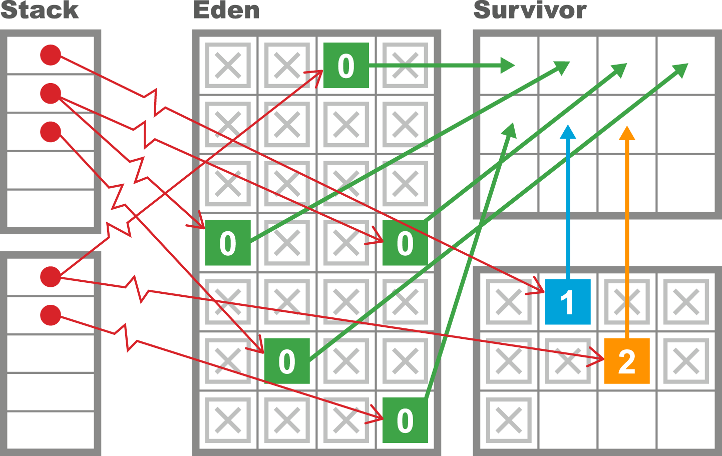
Figure 6-7. Collecting the young generation
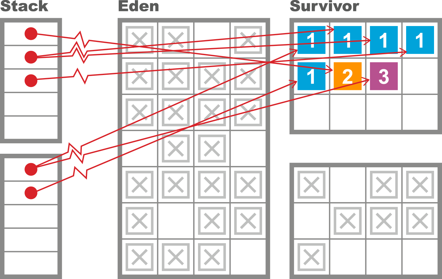
Figure 6-8. Evacuating the young generation
This approach attempts to take full advantage of the Weak Generational Hypothesis by touching only live objects. It also wants to be as efficient as possible and run using all cores as much as possible to shorten the STW pause time.
Old Parallel Collections
The ParallelOld collector is currently (as of Java 8) the default collector for the old generation. It has some strong similarities to Parallel GC, but also some fundamental differences. In particular, Parallel GC is a hemispheric evacuating collector, whereas ParallelOld is a compacting collector with only a single continuous memory space.
This means that as the old generation has no other space to be evacuated to, the parallel collector attempts to relocate objects within the old generation to reclaim space that may have been left by old objects dying. Thus, the collector can potentially be very efficient in its use of memory, and will not suffer from memory fragmentation.
This results in a very efficient memory layout at the cost of using a potentially large amount of CPU during full GC cycles. The difference between the two approaches can be seen in Figure 6-9.
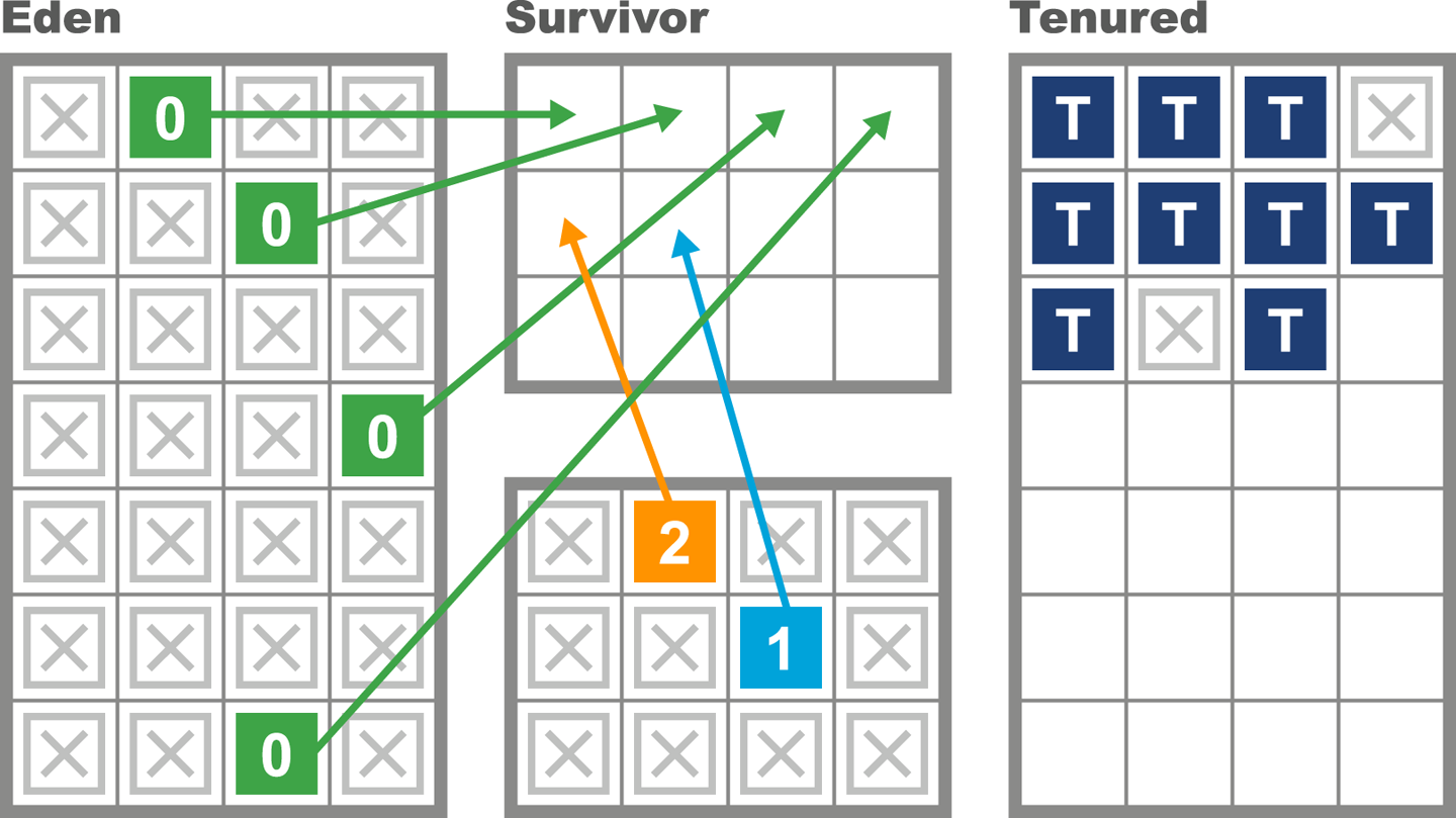
Figure 6-9. Evacuating versus compacting
The behavior of the two memory spaces is quite radically different, as they are serving different purposes. The purpose of the young collections is to deal with the short-lived objects, so the occupancy of the young space is changing radically with allocation and clearance at GC events.
By contrast, the old space does not change as obviously. Occasional large objects will be created directly in Tenured, but apart from that, the space will only change at collections—either by objects being promoted from the young generation, or by a full rescan and rearrangement at an old or full collection.
Limitations of Parallel Collectors
The parallel collectors deal with the entire contents of a generation at once, and try to collect as efficiently as possible. However, this design has some drawbacks. Firstly, they are fully stop-the-world. This is not usually an issue for young collections, as the Weak Generational Hypothesis means that very few objects should survive.
Note
The design of the young parallel collectors is such that dead objects are never touched, so the length of the marking phase is proportional to the (small) number of surviving objects.
This basic design, coupled with the usually small size of the young regions of the heap, means that the pause time of young collections is very short for most workloads. A typical pause time for a young collection on a modern 2 GB JVM (with default sizing) might well be just a few milliseconds, and is very frequently under 10 ms.
However, collecting the old generation is often a very different story. For one thing, the old generation is by default seven times the size of the young generation. This fact alone will make the expected STW length of a full collection much longer than for a young collection.
Another key fact is that the marking time is proportional to the number of live objects in a region. Old objects may be long-lived, so a potentially larger number of old objects may survive a full collection.
This behavior also explains a key weakness of parallel old collection—the STW time will scale roughly linearly with the size of the heap. As heap sizes continue to increase, ParallelOld starts to scale badly in terms of pause time.
Newcomers to GC theory sometimes entertain private theories that minor modifications to mark-and-sweep algorithms might help to alleviate STW pauses. However, this is not the case. Garbage collection has been a very well-studied research area of computer science for over 40 years, and no such “can’t you just…” improvement has ever been found.
As we will see in Chapter 7, mostly concurrent collectors do exist and they can run with greatly reduced pause times. However, they are not a panacea, and several fundamental difficulties with garbage collection remain.
As an example of one of the central difficulties with the naive approach to GC, let’s consider TLAB allocation. This provides a great boost to allocation performance but is of no help to collection cycles. To see why, consider this code:
publicstaticvoidmain(String[]args){int[]anInt=newint[1];anInt[0]=42;Runnabler=()->{anInt[0]++;System.out.println("Changed: "+anInt[0]);};newThread(r).start();}
The variable anInt is an array object containing a single int. It is allocated from a TLAB held by the main thread but immediately afterward is passed to a new thread. To put it another way, the key property of TLABs—that they are private to a single thread—is true only at the point of allocation. This property can be violated basically as soon as objects have been allocated.
The Java environment’s ability to trivially create new threads is a fundamental, and extremely powerful, part of the platform. However, it complicates the picture for garbage collection considerably, as new threads imply execution stacks, each frame of which is a source of GC roots.
The Role of Allocation
Java’s garbage collection process is most commonly triggered when memory allocation is requested but there is not enough free memory on hand to provide the required amount. This means that GC cycles do not occur on a fixed or predictable schedule but purely on an as-needed basis.
This is one of the most critical aspects of garbage collection: it is not deterministic and does not occur at a regular cadence. Instead, a GC cycle is triggered when one or more of the heap’s memory spaces are essentially full, and further object creation would not be possible.
Tip
This as-needed nature makes garbage collection logs hard to process using traditional time series analysis methods. The lack of regularity between GC events is an aspect that most time series libraries cannot easily accommodate.
When GC occurs, all application threads are paused (as they cannot create any more objects, and no substantial piece of Java code can run for very long without producing new objects). The JVM takes over all of the cores to perform GC, and reclaims memory before restarting the application threads.
To better understand why allocation is so critical, let’s consider the following highly simplified case study. The heap parameters are set up as shown, and we assume that they do not change over time. Of course a real application would normally have a dynamically resizing heap, but this example serves as a simple illustration.
| Heap area | Size |
|---|---|
Overall |
2 GB |
Old generation |
1.5 GB |
Young generation |
500 MB |
Eden |
400 MB |
S1 |
50 MB |
S2 |
50 MB |
After the application has reached its steady state, the following GC metrics are observed:
Allocation rate |
100 MB/s |
Young GC time |
2 ms |
Full GC time |
100 ms |
Object lifetime |
200 ms |
This shows that Eden will fill in 4 seconds, so at steady state, a young GC will occur every 4 seconds. Eden has filled, and so GC is triggered. Most of the objects in Eden are dead, but any object that is still alive will be evacuated to a survivor space (SS1, for the sake of discussion). In this simple model, any objects that were created in the last 200 ms have not had time to die, so they will survive. So, we have:
GC0 |
@ 4 s |
20 MB Eden → SS1 (20 MB) |
After another 4 seconds, Eden refills and will need to be evacuated (to SS2 this time). However, in this simplified model, no objects that were promoted into SS1 by GC0 survive—their lifetime is only 200 ms and another 4 s has elapsed, so all of the objects allocated prior to GC0 are now dead. We now have:
GC1 |
@ 8.002 s |
20 MB Eden → SS2 (20 MB) |
Another way of saying this is that after GC1, the contents of SS2 consist solely of objects newly arrived from Eden and no object in SS2 has a generational age > 1. Continuing for one more collection, the pattern should become clear:
GC2 |
@ 12.004 s |
20 MB Eden → SS1 (20 MB) |
This idealized, simple model leads to a situation where no objects ever become eligible for promotion to the Tenured generation, and the space remains empty throughout the run. This is, of course, very unrealistic.
Instead, the Weak Generational Hypothesis indicates that object lifetimes will be a distribution, and due to the uncertainty of this distribution, some objects will end up surviving to reach Tenured.
Let’s look at a very simple simulator for this allocation scenario. It allocates objects, most of which are very short-lived but some of which have a considerably longer life span. It has a couple of parameters that define the allocation: x and y, which between them define the size of each object; the allocation rate (mbPerSec); the lifetime of a short-lived object (shortLivedMS) and the number of threads that the application should simulate (nThreads). The default values are shown in the next listing:
publicclassModelAllocatorimplementsRunnable{privatevolatilebooleanshutdown=false;privatedoublechanceOfLongLived=0.02;privateintmultiplierForLongLived=20;privateintx=1024;privateinty=1024;privateintmbPerSec=50;privateintshortLivedMs=100;privateintnThreads=8;privateExecutorexec=Executors.newFixedThreadPool(nThreads);
Omitting main() and any other startup/parameter-setting code, the rest of the ModelAllocator looks like this:
publicvoidrun(){finalintmainSleep=(int)(1000.0/mbPerSec);while(!shutdown){for(inti=0;i<mbPerSec;i++){ModelObjectAllocationto=newModelObjectAllocation(x,y,lifetime());exec.execute(to);try{Thread.sleep(mainSleep);}catch(InterruptedExceptionex){shutdown=true;}}}}// Simple function to model Weak Generational Hypothesis// Returns the expected lifetime of an object - usually this// is very short, but there is a small chance of an object// being "long-lived"publicintlifetime(){if(Math.random()<chanceOfLongLived){returnmultiplierForLongLived*shortLivedMs;}returnshortLivedMs;}}
The allocator main runner is combined with a simple mock object used to represent the object allocation performed by the application:
publicclassModelObjectAllocationimplementsRunnable{privatefinalint[][]allocated;privatefinalintlifeTime;publicModelObjectAllocation(finalintx,finalinty,finalintliveFor){allocated=newint[x][y];lifeTime=liveFor;}@Overridepublicvoidrun(){try{Thread.sleep(lifeTime);System.err.println(System.currentTimeMillis()+": "+allocated.length);}catch(InterruptedExceptionex){}}}
When seen in VisualVM, this will display the simple sawtooth pattern that is often observed in the memory behavior of Java applications that are making efficient use of the heap. This pattern can be seen in Figure 6-10.
We will have a great deal more to say about tooling and visualization of memory effects in Chapter 7. The interested reader can steal a march on the tuning discussion by downloading the allocation and lifetime simulator referenced in this chapter, and setting parameters to see the effects of allocation rates and percentages of long-lived objects.
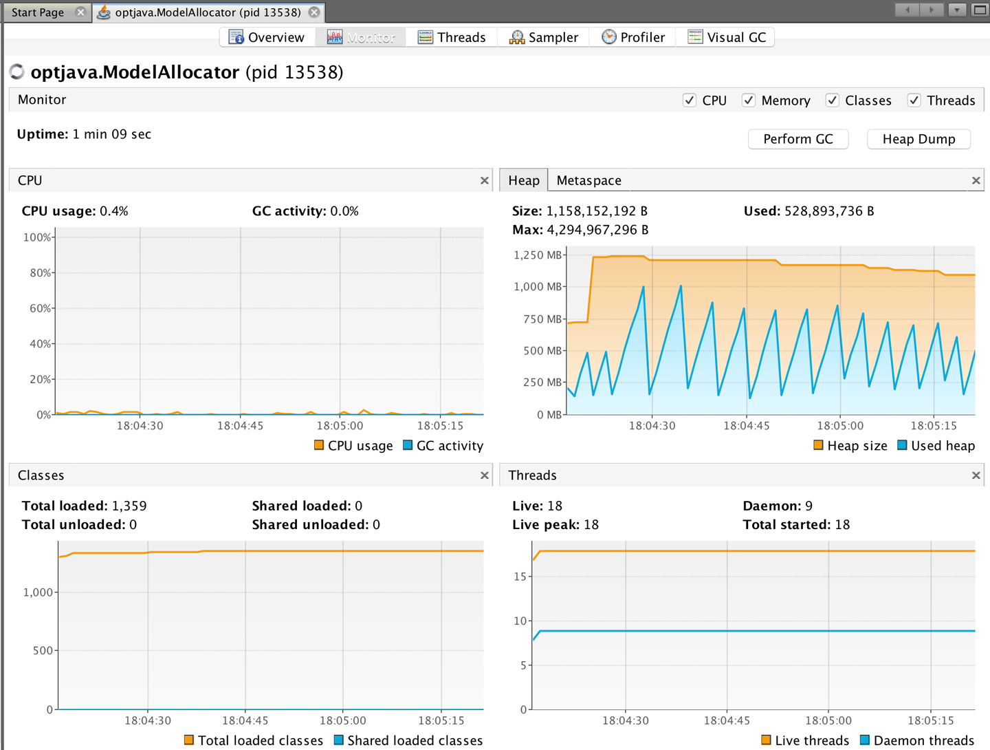
Figure 6-10. Simple sawtooth
To finish this discussion of allocation, we want to shift focus to a very common aspect of allocation behavior. In the real world, allocation rates can be highly changeable and “bursty.” Consider the following scenario for an application with a steady-state behavior as previously described:
2 s |
Steady-state allocation |
100 MB/s |
1 s |
Burst/spike allocation |
1 GB/s |
100 s |
Back to steady-state |
100 MB/s |
The initial steady-state execution has allocated 200 MB in Eden. In the absence of long-lived objects, all of this memory has a lifetime of 100 ms. Next, the allocation spike kicks in. This allocates the other 200 MB of Eden space in just 0.2 s, and of this, 100 MB is under the 100 ms age threshold. The size of the surviving cohort is larger than the survivor space, and so the JVM has no option but to promote these objects directly into Tenured. So we have:
GC0 |
@ 2.2 s |
100 MB Eden → Tenured (100 MB) |
The sharp increase in allocation rate has produced 100 MB of surviving objects, although note that in this model all of the “survivors” are in fact short-lived and will very quickly become dead objects cluttering up the Tenured generation. They will not be reclaimed until a full collection occurs.
Continuing for a few more collections, the pattern becomes clear:
GC1 |
@ 2.602 s |
200 MB Eden → Tenured (300 MB) |
GC2 |
@ 3.004 s |
200 MB Eden → Tenured (500 MB) |
GC2 |
@ 7.006 s |
20 MB Eden → SS1 (20 MB) [+ Tenured (500 MB)] |
Notice that, as discussed, the garbage collector runs as needed, and not at regular intervals. The bigger the allocation rate, the more frequent GCs are. If the allocation rate is too high, then objects will end up being forced to be promoted early.
This phenomenon is called premature promotion; it is one of the most important indirect effects of garbage collection and a starting point for many tuning exercises, as we will see in the next chapter.
Summary
The subject of garbage collection has been a live topic of discussion within the Java community since the platform’s inception. In this chapter, we have introduced the key concepts that performance engineers need to understand to work effectively with the JVM’s GC subsystem. These included:
-
Mark-and-sweep collection
-
HotSpot’s internal runtime representation for objects
-
The Weak Generational Hypothesis
-
Practicalities of HotSpot’s memory subsystems
-
The parallel collectors
-
Allocation and the central role it plays
In the next chapter, we will discuss GC tuning, monitoring, and analysis. Several of the topics we met in this chapter—especially allocation, and specific effects such as premature promotion—will be of particular significance to the upcoming goals and topics, and it may be helpful to refer back to this chapter frequently.
1 The System.gc() method exists, but is basically useless for any practical purpose.