Table of Contents for

Using SQLite

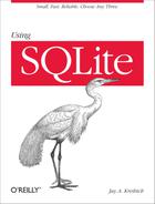
The most basic kind of inter-table relationship is the one-to-one relationship. As you can guess, this type of relationship establishes a reference from a single row in one table to a single row in another table. Most commonly, one-to-one relationships are represented by having a foreign key in one table reference a primary key in another table. If the foreign key column is made unique, only one reference will be allowed. As Figure 6-3 illustrates, a unique foreign key creates a one-to-one relationship between the rows of the two tables.

Figure 6-3. In a one-to-one relationship, table B has a foreign key that references the primary key of table A. This associates every non-NULL foreign key in table B with some row in table A.

In the strictest sense, a foreign key relationship is a one-to-(zero or one) relationship. When two tables are involved in a one-to-one relationship, there is nothing to enforce that every primary key has an incoming reference from a foreign key. For that matter, if the foreign key allows NULLs, there may be unassigned foreign keys as well.

One-to-one relationships are commonly used to create detail tables. As the name implies, a detail table typically holds details that are linked to the records in a more prominent table. Detail tables can be used to hold data that is only relevant to a small subsection of the database application. Breaking the detail data apart from the main tables allows different sections of the database design to evolve and grow much more independently.

Detail tables can also be helpful when extended data only applies to a limited number of records. For example, a website might have a sales_items table that lists common information (price, inventory, weight, etc.) for all available items. Type-specific data can then be held in detail tables, such as cd_info for CDs (artist name, album name, etc.) or dvd_info (directors, studio, etc.) for DVDs. Although the sales_items table would have a unique one-to-one relationship with every type-specific info table, each individual row in the sales_item table would be referenced by only one type of detail table.

One-to-one relationships can also be used to isolate very large data elements, such as BLOBs. Consider an employee database that contains an image of each employee. Due to the data storage and I/O overhead, it might be unwise to include a photo column directly in the employee table, but it is easy to create a photo table that references the employee table. Consider these two tables:

CREATE TABLE employee ( 
    employee_id  INTEGER   NOT NULL   PRIMARY KEY,
    name         TEXT   NOT NULL
    /* ...etc... */
);

CREATE TABLE employee_photo (
    employee_id  INTEGER   NOT NULL   PRIMARY KEY
                 REFERENCES employee,
    photo_data   BLOB
    /* ...etc... */
);

This example is a bit unique, because the employee_photo.employee_id column is both the primary key for the employee_photo table, as well as a foreign key to the employee table. Since we want a one-to-one relationship, it makes sense to just pair up primary keys. Because this foreign key does not allow NULL keys, every employee_photo row must be matched to a specific employee row. The database does not guarantee that every employee will have a matching employee_photo, however.

One-to-many relationships establish a link between a single row in one table to multiple rows in another table. This is done by expanding a one-to-one relationship, allowing one side to contain duplicate keys. One-to-many relationships are often used to associate lists or arrays of items back to a single row. For example, multiple shipping addresses can be linked to a single account. Unless otherwise specified, “many” usually means “zero or more.”

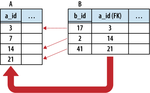
The only difference between a one-to-one relationship and a one-to-many relationship is that the one-to-many relationship allows for duplicate foreign key values. This allows multiple rows in one table (the many table) to refer back to a single row in another table (the One table). In building a one-to-many relationship, the foreign key must always be on the many side.

Figure 6-4 illustrates the relationship in more detail.

Figure 6-4. When building a one-to-many relationship, the primary keys must be unique, but foreign key columns may contain duplicate values. This means a one-to-many relationship must have the foreign key on the many side. Here we see a foreign key value in Table B refer to the primary key in Table A.

Any time you find yourself wondering how to stuff an array or list into the column of a table, the solution is to separate the array elements out into their own table and establish a one-to-many relationship.

The same is true any time you start to contemplate sets of columns, such as item0, item1, item2, etc., that are all designed to hold instances of the same type of value. Such designs have inherent limits, and the insert, update, and removal process becomes quite complex. It is much easier to just break the data out into its own table and establish a proper relationship.

One example of a one-to-many relationship is music albums, and the songs they contain. Each album has a list of songs associated with that album. For example:

CREATE TABLE albums (
        album_id INTEGER   NOT NULL   PRIMARY KEY,
        album_name TEXT );

CREATE TABLE tracks (
        track_id INTEGER   NOT NULL   PRIMARY KEY,
        track_name TEXT,
        track_number INTEGER,
        track_length INTEGER, -- in seconds
        album_id INTEGER   NOT NULL   REFERENCES albums );

Each album and track has a unique ID. Each track also has a foreign key reference back to its album. Consider:

INSERT INTO albums VALUES ( 1, "The Indigo Album" );
INSERT INTO tracks VALUES ( 1, "Metal Onion", 1, 137, 1 );
INSERT INTO tracks VALUES ( 2, "Smooth Snake", 2, 212, 1 );
INSERT INTO tracks VALUES ( 3, "Turn A", 3, 255, 1 );

INSERT INTO albums VALUES ( 2, "Morning Jazz" );
INSERT INTO tracks VALUES ( 4, "In the Bed", 1, 214, 2 );
INSERT INTO tracks VALUES ( 5, "Water All Around", 2, 194, 2 );
INSERT INTO tracks VALUES ( 6, "Time Soars", 3, 265, 2 );
INSERT INTO tracks VALUES ( 7, "Liquid Awareness", 4, 175, 2 );

To get a simple list of tracks and their associated album, we just join the tables back together. We can also sort by both album name and track number:

sqlite> SELECT album_name, track_name, track_number
   ...>   FROM albums JOIN tracks USING ( album_id )
   ...>   ORDER BY album_name, track_number;

album_name    track_name  track_number
------------  ----------  ------------
Morning Jazz  In the Bed  1           
Morning Jazz  Water All   2           
Morning Jazz  Time Soars  3           
Morning Jazz  Liquid Awa  4           
The Indigo A  Metal Onio  1           
The Indigo A  Smooth Sna  2           
The Indigo A  Turn A      3           

We can also manipulate the track groupings:

sqlite> SELECT album_name, sum( track_length ) AS runtime, count(*) AS tracks
   ...>   FROM albums JOIN tracks USING ( album_id )
   ...>   GROUP BY album_id;

album_name        runtime     tracks    
----------------  ----------  ----------
The Indigo Album  604         3         
Morning Jazz      848         4         

This query groups the tracks based off their album, and then aggregates the track data together.

The next step is the many-to-many relationship. A many-to-many relationship associates one row in the first table to many rows in the second table while simultaneously allowing individual rows in the second table to be linked to multiple rows in the first table. In a sense, a many-to-many relationship is really two one-to-many relationships built across each other.

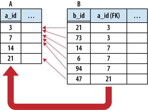
Figure 6-5 shows the classic many-to-many example of people and groups. One person can belong to many different groups, while each group is made up of many different people. Common operations are to find all the groups a person belongs to, or to find all the people in a group.

Figure 6-5. A many-to-many relationship is like two one-to-many relationships built across each other. In this example, each individual person can be a member of one or more groups, while each group can contain one or more people.

Many-to-many relationships are a bit more complex than other relationships. Although the tables have a many-to-many relationship with each other, the entries in both tables must remain unique. We cannot duplicate either person rows or group rows for the purpose of matching keys. This is a problem, since each foreign key can only reference one row. This makes it impossible for a foreign key of one table (such as a group) to refer to multiple rows of another table (such as people).

To solve this, we go back to the advice from before: if you need to add a list to a row, break out that list into its own table and establish a one-to-many relationship with the new table. You cannot directly represent a many-to-many relationship with only two tables, but you can take a pair of one-to-many relationships and link them together. The link requires a small table, known as a link table, or bridge table, that sits between the two many tables. Each many-to-many relationship requires a unique bridge table.

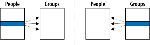
In its most basic form, the bridge table consists of nothing but two foreign keys—one for each of the tables it is linking together. Each row of the bridge table links one row in the first many table to one row in the second many table. In our People-to-Groups example, the link table defines a membership of one person in one group. This is illustrated in Figure 6-6.

Figure 6-6. Implementing a many-to-many relationship requires a bridge table. In this example, each row of the bridge table represents a membership of one person in one group. Note that the primary key of the bridge table is a multicolumn key over (p_id, g_id). This keeps memberships unique.

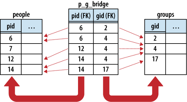
The logical representation of a many-to-many relationship is actually a one-to-many-to-one relationship, with the bridge table (acting as a record of membership) in the middle. Each person has a one-to-many relationship with memberships, just as groups have a one-to-many relationship with memberships. In addition to binding the two tables together, the bridge table can also hold additional information about the membership itself, such as a first-joined date or an expiration date.

Here are three tables. The people and groups table are obvious enough. The p_g_bridge table acts as the bridge table between the people table and groups table. The two columns are both foreign key references, one to people and one to groups. Establishing a primary key across both foreign key columns ensures the memberships remain unique:

CREATE TABLE people ( pid INTEGER   PRIMARY KEY, name TEXT, ... );
CREATE TABLE groups ( gid INTEGER   PRIMARY KEY, name TEXT, ... );
CREATE TABLE p_g_bridge( 
        pid INTEGER   NOT NULL   REFERENCES people,
        gid INTEGER   NOT NULL   REFERENCES groups,
        PRIMARY KEY ( pid, gid )
);

This query will list all the groups that a person belongs to:

SELECT groups.name AS group_name
  FROM people JOIN p_g_bridge USING ( pid ) JOIN groups USING ( gid )
  WHERE people.name = search_person_name;

The query simply links people to groups using the bridge table, and then filters out the appropriate rows.

We don’t always need all three tables. This query counts all the members of a group without utilizing the people table:

SELECT name AS group_name, count(*) AS members
  FROM groups JOIN p_g_bridge USING ( gid )
  GROUP BY gid;

There are many other queries we can do, like finding all the groups that have no members:

SELECT name AS group_name
  FROM groups LEFT OUTER JOIN p_g_bridge USING ( gid )
  WHERE pid IS NULL;

This query performs an outer join from the groups table to the p_g_bridge table. Any unmatched group rows will be padded out with a NULL in the p_g_bridge.pid column. Since this column is marked NOT NULL, we know the only possible way for a row to be NULL in that column is from the outer join, meaning the row is unmatched to any memberships. A very similar query could be used to find any people that have no memberships.

Hierarchies and other tree-style data relationships are common and frequently show up in database design. Modeling one in a database can be a challenge because you tend to ask different types of questions when dealing with hierarchies.

Common tree operations include finding all the sub-nodes under a given node, or querying the depth of a given node. These operations have an inherent recursion in them—a concept that SQL doesn’t support. This can lead to clumsy queries or complex representations.

There are two common methods for representing a tree relation using database tables. The first is the adjacency model, which uses a simple representation that is easy to modify but complex to query. The other common representation is the nested set, which allows relatively simple queries, but at the cost of a more complex representation that can be expensive to modify.

CREATE TABLE tree (
    node   INTEGER   NOT NULL   PRIMARY KEY,
    name   TEXT,
    parent INTEGER   REFERENCES tree );

A
  A.1
    A.1.a
  A.2
    A.2.a
    A.2.b
  A.3

INSERT INTO tree VALUES ( 1, 'A',     NULL );
INSERT INTO tree VALUES ( 2, 'A.1',   1 );
INSERT INTO tree VALUES ( 3, 'A.1.a', 2 );
INSERT INTO tree VALUES ( 4, 'A.2',   1 );
INSERT INTO tree VALUES ( 5, 'A.2.a', 4 );
INSERT INTO tree VALUES ( 6, 'A.2.b', 4 );
INSERT INTO tree VALUES ( 7, 'A.3',   1 );

sqlite> SELECT n.name AS node, p.name AS parent
   ...>   FROM tree AS n JOIN tree AS p ON n.parent = p.node;

node        parent    
----------  ----------
A.1         A         
A.1.a       A.1       
A.2         A         
A.2.a       A.2       
A.2.b       A.2       
A.3         A         

CREATE TABLE nest (
    name  TEXT,
    lower INTEGER   NOT NULL   UNIQUE,
    upper INTEGER   NOT NULL   UNIQUE,
    CHECK ( lower < upper ) );

A( A.1( A.1.a( ) ), A.2( A.2.a( ), A.2.b( )  ), A.3(  )  )
 1    2      3 4 5     6      7 8       9 10 11    12 13 14

INSERT INTO nest VALUES ( 'A',      1, 14 );
INSERT INTO nest VALUES ( 'A.1',    2,  5 );
INSERT INTO nest VALUES ( 'A.1.a',  3,  4 );
INSERT INTO nest VALUES ( 'A.2',    6, 11 );
INSERT INTO nest VALUES ( 'A.2.a',  7,  8 );
INSERT INTO nest VALUES ( 'A.2.b',  9, 10 );
INSERT INTO nest VALUES ( 'A.3',   12, 13 );

SELECT name FROM nest WHERE lower + 1 = upper;

sqlite> SELECT n.name AS name, count(*) AS depth
   ...>   FROM nest AS n JOIN nest AS p
   ...>     ON p.lower <= n.lower AND p.upper >= n.upper
   ...>   GROUP BY n.name;

name        depth     
----------  ----------
A           1         
A.1         2         
A.1.a       3         
A.2         2         
A.2.a       3         
A.2.b       3         
A.3         2