

Beijing • Cambridge • Farnham • Köln • Sebastopol • Tokyo
To my Great-Uncle Albert “Unken Al” Kreibich.
1918–1994
He took a young boy whose favorite question was “why?” and taught him to ask the question “how?”
(Who also—much to the dismay of his parents and the kitchen telephone—taught him the joy of answering that question, especially if it involved pliers or screwdrivers.)
— jk
Supplemental files and examples for this book can be found at http://examples.oreilly.com/9780596521196/. Please use a standard desktop web browser to access these files, as they may not be accessible from all ereader devices.
All code files or examples referenced in the book will be available online. For physical books that ship with an accompanying disc, whenever possible, we’ve posted all CD/DVD content. Note that while we provide as much of the media content as we are able via free download, we are sometimes limited by licensing restrictions. Please direct any questions or concerns to booktech@oreilly.com.
This book provides an introduction to the SQLite database product. SQLite is a zero-configuration, standalone, relational database engine that is designed to be embedded directly into an application. Database instances are self-contained within a single file, allowing easy transport and simple setup.
Using SQLite is primarily written for experienced software developers that have never had a particular need to learn about relational databases. For one reason or another, you now find yourself with a large data management task, and are hoping a product like SQLite may provide the answer. To help you out, the various chapters cover the SQL language, the SQLite C programming API, and the basics of relational database design, giving you everything you need to successfully integrate SQLite into your applications and development work.
The book is divided into two major sections. The first part is a traditional set of chapters that are primarily designed to be read in order. The first two chapters provide an in-depth look at exactly what SQLite provides and how it can be used. The third chapter covers downloading and building the library. Chapters Four and Five provide an introduction to the SQL language, while Chapter Six covers database design concepts. Chapter Seven covers the basics of the C API. Chapter Eight builds on that to cover more advanced topics, such as storing times and dates, using SQLite from scripting languages, and utilizing some of the more advanced extensions. Chapters Nine and Ten cover writing your own custom SQL functions, extensions, and modules.
To complete the picture, the ten chapters are followed by several reference appendixes. These references cover all of the SQL commands, expressions, and built-in functions supported by SQLite, as well as documentation for the complete SQLite API.
The first edition of this book coves SQLite version 3.6.23.1. As this goes to press, work on SQLite version 3.7 is being finalized. SQLite 3.7 introduces a new transaction journal mode known as Write Ahead Logging, or WAL. In some environments, WAL can provide better concurrent transaction performance than the current rollback journal. This performance comes at a cost, however. WAL has more restrictive operational requirements and requires more advanced support from the operating system.
Once WAL has been fully tested and released, look for an article on the O’Reilly website that covers this new feature and how to get the most out of it.
The SQLite project maintains three mailing lists. If you’re trying to learn more about SQLite, or have any questions that are not addressed in this book or in the project documentation, these are often a good place to start.
This list is limited to announcements of new releases, critical bug alerts, and other significant events in the SQLite community. Traffic is extremely low, and most messages are posted by the SQLite development team.
This is the main support list for SQLite. It covers a broad range of topics, including SQL questions, programming questions, and questions about how the library works. This list is moderately busy.
This list is for people working on the internal code of the SQLite library itself. If you have questions about how to use the published SQLite API, those questions belong on the sqlite-users list. Traffic on this list is fairly low.
You can find instructions on how to join these mailing lists on the SQLite website. Visit http://www.sqlite.org/support.html for more details.
The sqlite-users@sqlite.org email list can be quite helpful, but it is a moderately busy list. If you’re only a casual user and don’t wish to receive that much email, you can also access and search list messages through a web archive. Links to several different archives are available on the SQLite support page.
The code examples found in this book are available for download from the O’Reilly website. You can find a link to the examples on the book’s catalog page at http://oreilly.com/catalog/9780596521196/. The files include both the SQL examples and the C examples found in later chapters.
Taking a book from an idea to a finished product involves a great many people. Although my name is on the cover, this could not have been possible without all of their help.
First, I would like to acknowledge the friendship and support of my primary editor, Mike Loukides. Thanks to some mutual friends, I first started doing technical reviews for Mike over eight years ago. Through the years, Mike gently encouraged me to take on my own project.
The first step on that path came nearly three years ago. I had downloaded a set of database exports from the Wikipedia project and was trying to devise a minimal database configuration that would (hopefully) cram nearly all the current data onto a small flash storage card. The end goal was to provide a local copy of the Wikipedia articles on an ebook reader I had. SQLite was a natural choice. At some point, frustrated with trying to understand the correct call sequence, I threw my hands up and exclaimed, “Someone should write a book about this!”—Ding!—The proverbial light bulb went off, and many, many (many…) late nights later, here we are.
Behind Mike stands the whole staff of O’Reilly Media. Everyone I interacted with did their best to help me out, calm me down, and fix my problems—sometimes all at once. The production staff understands how to make life easy for the author, so that we can focus on writing and leave the details to someone else.
I would like to thank D. Richard Hipp, the creator and lead maintainer of SQLite. In addition to coordinating the continued development of SQLite and providing us all with a high-quality software product, he was also gracious enough to answer numerous questions, as well as review a final draft of the manuscript. Some tricky spots went through several revisions, and he was always quick to review things and get back to me with additional comments.
A technical review was also done by Jon W. Marks. Jon is an old personal and professional friend with enterprise-class database experience. He has had the opportunity to mentor several experienced developers as they made their first journey into the relational database world. Jon provided very insightful feedback, and was able to pinpoint areas that are often difficult for beginners to grasp.
My final two technical reviewers were Jordan Hawker and Erin Moy. Although they are knowledgeable developers, they were relatively new to relational databases. As they went through the learning process, they kept me honest when I started to make too many assumptions, and kept me on track when I started to skip ahead too quickly.
I also owe a thank-you to Mike Kulas and all my coworkers at Volition, Inc. In addition to helping me find the right balance between my professional work and the book work, Mike helped me navigate our company’s intellectual property policies, making sure everything was on the straight and narrow. Numerous coworkers also deserve a thank-you for reviewing small sections, looking at code, asking lots of good questions, and otherwise putting up with me venting about not having enough time in the day.
A tip of the hat goes out to the crew at the Aroma Café in downtown Champaign, Illinois. They’re just a few blocks down from my workplace, and a significant portion of this book was written at their coffee shop. Many thanks to Michael and his staff, including Kim, Sara, Nichole, and Jerry, for always having a hot and creamy mocha ready.
Finally, I owe a tremendous debt to my wife, Debbie Fligor, and our two sons. They were always willing to make time for me to write and showed enormous amounts of patience and understanding. They all gave more than I had any right to ask, and this accomplishment is as much theirs as it is mine.
The following typographical conventions are used in this book:
Indicates new terms, URLs, email addresses, filenames, and file extensions.
Constant width
Used for program listings, as well as within paragraphs to refer to program elements such as variable or function names, databases, data types, environment variables, statements, and keywords.
Constant width bold
Shows commands or other text that should be typed literally by the user.
Constant width italic
Shows text that should be replaced with user-supplied values or by values determined by context.
This book is here to help you get your job done. In general, you may use the code in this book in your programs and documentation. You do not need to contact us for permission unless you’re reproducing a significant portion of the code. For example, writing a program that uses several chunks of code from this book does not require permission. Selling or distributing a CD-ROM of examples from O’Reilly books does require permission. Answering a question by citing this book and quoting example code does not require permission. Incorporating a significant amount of example code from this book into your product’s documentation does require permission.
We appreciate, but do not require, attribution. An attribution usually includes the title, author, publisher, and ISBN. For example: “Using SQLite by Jay A. Kreibich. Copyright 2010 O’Reilly Media, Inc., 978-0-596-52118-9.”
If you feel your use of code examples falls outside fair use or the permission given above, feel free to contact us at permissions@oreilly.com.
Safari Books Online is an on-demand digital library that lets you easily search over 7,500 technology and creative reference books and videos to find the answers you need quickly.
With a subscription, you can read any page and watch any video from our library online. Read books on your cell phone and mobile devices. Access new titles before they are available for print, and get exclusive access to manuscripts in development and post feedback for the authors. Copy and paste code samples, organize your favorites, download chapters, bookmark key sections, create notes, print out pages, and benefit from tons of other time-saving features.
O’Reilly Media has uploaded this book to the Safari Books Online service. To have full digital access to this book and others on similar topics from O’Reilly and other publishers, sign up for free at http://my.safaribooksonline.com.
Please address comments and questions concerning this book to the publisher:
| O’Reilly Media, Inc. |
| 1005 Gravenstein Highway North |
| Sebastopol, CA 95472 |
| 800-998-9938 (in the United States or Canada) |
| 707-829-0515 (international or local) |
| 707 829-0104 (fax) |
We have a web page for this book, where we list errata, examples, and any additional information. You can access this page at:
| http://oreilly.com/catalog/9780596521196/ |
To comment or ask technical questions about this book, send email to:
| bookquestions@oreilly.com |
For more information about our books, conferences, Resource Centers, and the O’Reilly Network, see our web site at:
| http://www.oreilly.com |
In the simplest terms, SQLite is a public-domain software package that provides a relational database management system, or RDBMS. Relational database systems are used to store user-defined records in large tables. In addition to data storage and management, a database engine can process complex query commands that combine data from multiple tables to generate reports and data summaries. Other popular RDBMS products include Oracle Database, IBM’s DB2, and Microsoft’s SQL Server on the commercial side, with MySQL and PostgreSQL being popular open source products.
The “Lite” in SQLite does not refer to its capabilities. Rather, SQLite is lightweight when it comes to setup complexity, administrative overhead, and resource usage. SQLite is defined by the following features:
SQLite does not require a separate server process or system to operate. The SQLite library accesses its storage files directly.
No server means no setup. Creating an SQLite database instance is as easy as opening a file.
The entire database instance resides in a single cross-platform file, requiring no administration.
A single library contains the entire database system, which integrates directly into a host application.
The default build is less than a megabyte of code and requires only a few megabytes of memory. With some adjustments, both the library size and memory use can be significantly reduced.
SQLite transactions are fully ACID-compliant, allowing safe access from multiple processes or threads.
SQLite supports most of the query language features found in the SQL92 (SQL2) standard.
The SQLite development team takes code testing and verification very seriously.
Overall, SQLite provides a very functional and flexible relational database environment that consumes minimal resources and creates minimal hassle for developers and users.
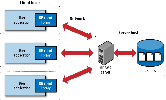
Unlike most RDBMS products, SQLite does not have a client/server architecture. Most large-scale database systems have a large server package that makes up the database engine. The database server often consists of multiple processes that work in concert to manage client connections, file I/O, caches, query optimization, and query processing. A database instance typically consists of a large number of files organized into one or more directory trees on the server filesystem. In order to access the database, all of the files must be present and correct. This can make it somewhat difficult to move or reliably back up a database instance.
All of these components require resources and support from the host computer. Best practices also dictate that the host system be configured with dedicated service-user accounts, startup scripts, and dedicated storage, making the database server a very intrusive piece of software. For this reason, and for performance concerns, it is customary to dedicate a host computer system solely for the database server software.
To access the database, client software libraries are typically provided by the database vendor. These libraries must be integrated into any client application that wishes to access the database server. These client libraries provide APIs to find and connect to the database server, as well as set up and execute database queries and commands. Figure 1-1 shows how everything fits together in a typical client/server RDBMS.
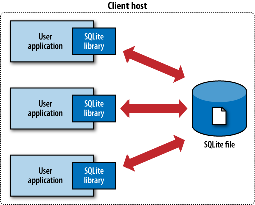
In contrast, SQLite has no separate server. The entire database engine is integrated into whatever application needs to access a database. The only shared resource among applications is the single database file as it sits on disk. If you need to move or back up the database, you can simply copy the file. Figure 1-2 shows the SQLite infrastructure.
By eliminating the server, a significant amount of complexity is removed. This simplifies the software components and nearly eliminates the need for advanced operating system support. Unlike a traditional RDBMS server that requires advanced multitasking and high-performance inter-process communication, SQLite requires little more than the ability to read and write to some type of storage.
This simplicity makes it fairly straightforward to port SQLite to just about any environment, including mobile phones, handheld media players, game consoles, and other devices, where no traditional database system could ever dare to venture.
Although SQLite does not use a traditional client/server architecture, it is common to speak of applications being “SQLite clients.” This terminology is often used to describe independent applications that simultaneously access a shared SQLite database file, and is not meant to imply that there is a separate server.
SQLite is designed to be integrated directly into an executable. This eliminates the need for an external library and simplifies distribution and installation. Removing external dependencies also removes most versioning issues. If the SQLite code is built right into your application, you never have to worry about linking to the correct version of a client library, or that the client library is version-compatible with the database server.
Eliminating the server imposes some restrictions, however. SQLite is designed to address localized storage needs, such as a web server accessing a local database. This means it isn’t well suited for situations where multiple client machines need to access a centralized database. That situation is more representative of a client/server architecture, and is better serviced by a database system that uses the same architecture.
SQLite packages the entire database into a single file. That single file contains the database layout as well as the actual data held in all the different tables and indexes. The file format is cross-platform and can be accessed on any machine, regardless of native byte order or word size.
Having the whole database in a single file makes it trivial to create, copy, or back up the on-disk database image. Whole databases can be emailed to colleagues, posted to a web forum, or checked into a revision control system. Entire databases can be moved, modified, and shared with the same ease as a word-processing document or spread-sheet file. There is no chance of a database becoming corrupt or unavailable because one of a dozen files was accidentally moved or renamed.
Perhaps most importantly, computer users have grown to expect that a document, project, or other “unit of application data” is stored as a single file. Having the whole database in a single file allows applications to use database instances as documents, data stores, or preference data, without contradicting customer expectations.
From an end-user standpoint, SQLite requires nothing to install, nothing to configure, and nothing to worry about. While there are a fair number of tuning parameters available to developers, these are normally hidden from the end-user. By eliminating the server and merging the database engine directly into your application, your customers never need to know they’re using a database. It is quite practical to design an application so that selecting a file is the only customer interaction—an action they are already comfortable doing.
SQLite’s small code size and conservative resource use makes it well suited for embedded systems running limited operating systems. The ANSI C source code tends toward an older, more conservative style that should be accepted by even the most eccentric embedded processor compiler. Using the default configuration, the compiled SQLite library is less than 700 KB on most platforms, and requires less than 4 MB of memory to operate. By omitting the more advanced features, the library can often be trimmed to 300 KB or less. With minor configuration changes, the library can be made to function on less than 256 KB of memory, making its total footprint not much more than half a megabyte, plus data storage.
SQLite expects only minimal support from its host environment and is written in a very modular way. The internal memory allocator can be easily modified or swapped out, while all file and storage access is done through a Virtual File System (VFS) interface that can be modified to meet the needs and requirements of different platforms. In general, SQLite can be made to run on almost anything with a 32-bit processor.
SQLite offers several features not found in many other database systems. The most notable difference is that SQLite uses a dynamic-type system for tables. The SQLite engine will allow you to put any value into nearly any column, regardless of type. This is a major departure from traditional database systems, which tend to be statically typed. In many ways, the dynamic-type system in SQLite is similar to those found in popular scripting languages, which often have a single scalar type that can accept anything from integers to strings. In my own experience, the dynamic-type system has solved many more problems than it has caused.
Another useful feature is the ability to manipulate more than one database at a time. SQLite allows a single database connection to associate itself with multiple database files simultaneously. This allows SQLite to process SQL statements that bridge across multiple databases. This makes it trivial to join tables from different databases with a single query, or bulk copy data with a single command.
SQLite also has the ability to create fully in-memory databases. These are essentially database “files” that have no backing store and spend their entire lifetime within the file cache. While in-memory databases lack durability and do not provide full transaction support, they are very fast (assuming you have enough RAM), and are a great place to store temporary tables and other transient data.
There are a number of other features that make SQLite extremely flexible. Many of these, like virtual tables, are based off similar features found in other products, but with their own unique twist. These features and extensions provide a number of powerful tools to adapt SQLite to your own particular problem or situation.
SQLite, and the SQLite code, have no user license. It is not covered by the GNU General Public License (GPL) or any of the similar open source/free-source licenses. Rather, the SQLite development team has chosen to place the SQLite source code in the public domain. This means that they have explicitly and deliberately relinquished any claim they have to copyright or ownership of the code or derived products.
In short, this basically means you can do whatever you want with the SQLite source code, short of claiming to own it. The code and compiled libraries can be used in any way, modified in any way, redistributed in any way, and sold in any way. There are no restrictions, and no requirements or obligations to make third-party changes or modifications available to the project or the public.
The SQLite team takes this decision very seriously. Great care is taken to avoid any potential software patents or patented algorithms. All contributions to the SQLite source require a formal copyright release. Commercial contributions also require signed affidavits stating that the authors (and, if applicable, their employers) release their work into the public domain.
All of this effort is taken to ensure that integrating SQLite into your product carries along minimal legal baggage or liability, making it a viable option for almost any development effort.
The purpose of a database is to keep your data safe and organized. The SQLite development team is aware that nobody will use a database product that has a reputation for being buggy or unreliable. To maintain a high level of reliability, the core SQLite library is aggressively tested before each release.
In full, the standard SQLite test suites consists of over 10 million unit tests and query tests. The “soak test,” done prior to each release, consists of over 2.5 billion tests. The suite provides 100% statement coverage and 100% branch coverage, including edge-case errors, such as out-of-memory and out-of-storage conditions. The test suite is designed to push the system to its specified limits and beyond, providing extensive coverage of both code and operating parameters.
This high level of testing keeps the SQLite bug count relatively low. No software is perfect, but bugs that contribute to actual data-loss or database corruption are fairly rare. Most bugs that escape are performance related, where the database will do the right thing, but in the wrong way, leading to longer run-times.
Strong testing also keeps backwards compatibility extremely solid. The SQLite team takes backwards compatibility very seriously. File formats, SQL syntax, and programming APIs and behaviors have an extremely strong history of backwards compatibility. Updating to a new version of SQLite rarely causes compatibility problems.
In addition to keeping the core library reliable, the extensive testing also frees the SQLite developers to be more experimental. Whole subsystems of the SQLite code can be (and have been) ripped out and updated or replaced, with little concern about compatibility or functional differences—as long as all the tests pass. This allows the team to make significant changes with relatively little risk, constantly pushing the product and performance forward.
Like so many other aspects of the SQLite design, fewer bugs means fewer problems and less to worry about. As much as any complex piece of software can, it just works.
SQLite is remarkably flexible in both where it can be run and how it can be used. This chapter will take a brief look at some of the roles SQLite is designed to fill. Some of these roles are similar to those taken by traditional client/server RDBMS products. Other roles take advantage of SQLite’s size and ease of use, offering solutions you might not consider with a full client/server database.
Years of experience has taught developers that large client/server RDBMS platforms are powerful tools for safely storing, organizing, and manipulating data. Unfortunately, most large RDBMS products are resource-intensive and require a lot of upkeep. This boosts their performance and capacity, but it also limits how and where they can be practically deployed.
SQLite is designed to fill in those gaps, providing the same powerful and familiar tools for safely storing, organizing, and manipulating data in smaller, more resource constrained environments. SQLite is designed to complement, rather than replace, larger RDBMS platforms in situations where simplicity and ease of use are more important than capacity and concurrency.
This complimentary role enables applications and tools to embrace relational data management (and the years of experience that come with it), even if they’re running on smaller platforms without administrative oversight. Developers may laugh at the idea of installing MySQL on a desktop system (or mobile phone!) just to support an address book application, but with SQLite this not only becomes possible, it becomes entirely practical.
Modern desktop applications typically deal with a significant number of files. Most applications and utilities have one or more preference files. There may also be system-wide and per-user configuration files, caches, and other data that must be tracked and stored. Document-based applications also need to store and access the actual document files.
Using the SQLite library as an abstract storage layer has many advantages. A fair amount of application metadata, such as caches, state data, and configuration data, fit well with the relational data model. This makes it relatively easy to create an appropriate database design that maps cleanly and easily into an application’s internal data structures.
In many cases, SQLite can also work well as a document file format. Rather than creating a custom document format, an application can simply use individual database instances to represent working documents. SQLite supports many standard datatypes, including Unicode text, as well as arbitrary binary data fields that can store images or other raw data.
Even if an application does not have particularly strong relational requirements, there are still significant advantages to using the SQLite library as a storage container. The SQLite library provides incremental updates that make it quick and easy to save small changes. The transaction system protects all file I/O against process termination and power disruption, nearly eliminating the possibility of file corruption. SQLite even provides its own file caching layer, so that very large files can be opened and processed in a limited memory footprint, without any additional work on the part of the application.
SQLite database files are cross-platform, allowing easy migration. File contents can be easily and safely shared with other applications without worrying about detailed file format specifications. The common file format also makes it easy for automated scripts or troubleshooting utilities to access the files. Multiple applications can even access the same file simultaneously, and the library will transparently take care of all required file locking and cache synchronization.
The use of SQLite can also make debugging and troubleshooting much easier, as files can be inspected and manipulated with standard database tools. You can even use standard tools to inspect and modify a database file as your application is using it. Similarly, test files can be programmatically generated outside the application, which is useful for automatic testing suites.
Using an entire database instance as a document container may sound a bit unusual, but it is worth considering. The advantages are significant and should help a developer stay focused on the core of their application, rather than worrying about file formats, caching, or data synchronization.
SQLite is capable of creating databases that are held entirely in memory. This is extremely useful for creating small, temporary databases that require no permanent storage.
In-memory databases are often used to cache results pulled from a more traditional RDBMS server. An application may pull a subset of data from the remote database, place it into a temporary database, and then process multiple detailed searches and refinements against the local copy. This is particularly useful when processing type-ahead suggestions, or any other interactive element that requires very quick response times.
Temporary databases can also be used to index and store nearly any type of inter-linked, cross-referenced data. Rather than designing a set of complex runtime data structures which might include multiple hash tables, trees, and cross-referenced pointers, the developer can simply design an appropriate database schema and load the data into the database.
While it might seem odd to execute SQL statements in order to extract data from an in-memory data structure, it is surprisingly efficient and can reduce development time and complexity. A database also provides an upgrade path, making it trivial to grow the data beyond the available memory or persist the data across application runs, simply by migrating to an on-disk database.
SQLite makes it very easy to package complex data sets into a single, easy-to-access, fully cross-platform file. Having all the data in a single file makes it much easier to distribute or download large, multi-table data stores, such as large dictionaries or geo-location references.
Unlike many RDBMS products, the SQLite library is able to access read-only database files. This allows data stores to be read directly from an optical disc or other read-only filesystem. This is especially useful for systems with limited hard drive space, such as video game consoles.
SQLite works well as a “stand-in” database for those situations when a more robust RDBMS would normally be the right choice, were it available. SQLite can be especially useful for the demonstration and evaluation of applications and tools that normally depend on a database.
Consider a data analysis product that is designed to pull data from a relational database to generate reports and graphs. It can be difficult to offer downloads and evaluation copies of such software. Even if a download is available, the software must be configured and authorized to connect to a database that contains applicable data. This presents a significant barrier for a potential customer.
Now consider an evaluation download that includes support for a bundled SQLite demonstration database. By simply downloading and running the software, customers can interact and experiment with the sample database. This makes the barrier of entry significantly lower, allowing a customer to go from downloading to running data in just a few seconds.
Similar concerns apply to traditional sales and marketing demonstrations. Reliable network connectivity is often unavailable when doing on-site demonstrations to potential clients, so it is standard practice to run a local database server for demonstration purposes. Running a local database server consumes significant resources and adds administrative overhead. Database licenses may also be a concern.
The use of SQLite eliminates these issues. The database becomes a background piece, allowing the demonstration to focus on the product. There are no database administration concerns. The simple file format also makes it easy to prepare customer-specific data sets or show off product features that significantly modify the database. All this can be done by simply making a copy of the database file before proceeding.
Beyond evaluations and demonstrations, SQLite support can be used to promote a “lite” or “personal edition” of a larger product. Adding an entry-level product that is more suitable and cost-effective for smaller installations can open up a significant number of new customers by providing a low-cost, no-fuss introduction to the product line.
SQLite support can even help with development and testing. SQLite databases are small and compact, allowing them to be attached to bug reports. They also provide an easy way to test a wide variety of situations, allowing a product to be tested against hundreds, if not thousands, of unique database instances. Even if a customer never sees an SQLite database, the integration time may easily pay for itself with improved testing and debugging capabilities.
For the student looking to learn SQL and the basics of the relational model, SQLite provides an extremely accessible environment that is easy to set up, easy to use, and easy to share. SQLite offers a full-fledged relational system that supports nearly all of the core SQL language, yet requires no server setup, no administration, and no overhead. This allows students to focus on learning SQL and data manipulation without getting bogged down by server configuration and database maintenance.
Given its compact size, it is simple to place a Windows, Mac OS X, and Linux version of the command-line tools, along with several databases, onto a small flash drive. With no installation process and fully cross-platform database files, this provides an “on the go” teaching environment that will work with nearly any computer.
The “database in a file” architecture makes it easy for students to share their work. Whole database instances can be attached to an email or posted to a discussion forum. The single-file format also makes it trivial to back up work in progress, allowing students to experiment and explore different solutions without concern over losing data.
SQLite virtual tables allow a developer to define the contents of a table through code. By defining a set of callback functions that fetch and return rows and columns, a developer can create a link between the SQLite data processing engine and any data source. This allows SQLite to run queries against the data source without importing the data into a standard table.
Virtual tables are an extremely useful way to generate reports or allow ad hoc queries against logs or any tabular data set. Rather than writing a set of custom search or reporting tools, the data can simply be exposed to the SQLite engine. This allows reports and queries to be expressed in SQL, a language that many developers are already familiar with using. It also enables the use of generic database visualization tools and report generators.
Chapter 10 shows how to build a virtual table module that provides direct access to live web server logs.
Although SQLite has proven itself extremely flexible, there are some roles that are outside of its design goals. While SQLite may be able to perform in these areas, it might not be the best fit. If you find yourself with any of these requirements, it may be more practical to consider a more traditional client/server RDBMS product.
SQLite is able to support moderate transaction rates, but it is not designed to support the level of concurrent access provided by many client/server RDBMS products. Many server systems are able to provide table-level or row-level locking, allowing multiple transactions to be processed in parallel without the risk of data loss.
The concurrency protection offered by SQLite depends on file locks to protect against data loss. This model allows multiple database connections to access a database at the same time, but the whole database file must be locked in an exclusive mode to make any changes. As a result, write transactions are serialized across all database connections, limiting the overall transaction rate.
Depending on the size and complexity of your updates, SQLite might be able to handle a few hundred transactions per minute from different processes or threads. If, however, you start to see performance problems, or expect higher transaction rates, a client/server system is likely to provide better transaction performance.
It is not unusual to find SQLite databases that approach a dozen gigabytes or more, but there are some practical limits to the amount of data that can (or should) be stuffed into an SQLite database. Because SQLite puts everything into a single file (and thus, a single filesystem), very large data sets can stress the capability of the operating system or filesystem design. Although most modern filesystems are capable of handling files that are a terabyte or larger, that doesn’t always mean they’re very good at it. Many filesystems see a significant drop in performance for random access patterns if the file starts to get into multiple gigabyte ranges.
If you need to store and process several gigabytes or more of data, it might be wise to consider a more performance-oriented product.
An SQLite database has no authentication or authorization data. Instead, SQLite depends on filesystem permissions to control access to the raw database file. This essentially limits access to one of three states: complete read/write access, read-only access, or no access at all. Write access is absolute, and allows both data modification and the ability to alter the structure of the database itself.
While the SQLite API provides a basic application-layer authorization mechanism, it is trivial to circumvent if the user has direct access to the database file. Overall, this makes SQLite unsuitable for sensitive data stores that require per-user access control.
SQLite is specifically designed without a network component, and is best used as a local resource. There is no native support for providing access to multiple computers over a network, making it a poor choice as a client/server database system.
Having multiple computers access an SQLite file through a shared directory is also problematic. Most networked filesystems have poor file-locking facilities. Without the ability to properly lock the file and keep updates synchronized, the database file can easily become corrupt.
This isn’t to say that client/server systems can’t utilize SQLite. For example, many web servers utilize SQLite. This works because all of the web server processes are running on the same machine and are all accessing the database file from local storage.
SQLite has no internal support for database replication or redundancy. Simple replication can be achieved by copying the database file, but this must be done when nothing is attempting to modify the database.
Replication systems can be built on top of the basic database API, but such systems tend to be somewhat fragile. Overall, if you’re looking for real-time replication—especially at a transaction-safe level—you’ll need to look at a more complex RDBMS platform.
Most of these requirements get into a realm where complexity and administrative overhead is traded for capacity and performance. This makes sense for a large client/server RDBMS platform, but it is somewhat at odds with the SQLite design goals of staying simple and maintenance free. To keep frustration to a minimum, use the right tool for the job.
The SQLite website states that, “SQLite is the most widely deployed SQL database engine in the world.” This is a pretty bold claim, especially considering that when most people think of relational database platforms, they usually think of names like Oracle, SQL Server, and MySQL.
It is also a claim that is difficult to support with exact numbers. Because there are no license agreements or disclosure requirements, it is hard to guess just how many SQLite databases are out there. Nobody, including the SQLite development team, is fully aware of who is using SQLite, and for what purposes.
Regardless, the list of known SQLite users adds up to an impressive list. The Firefox web browser and the Thunderbird email client both use several SQLite databases to store cookies, history, preferences, and other account data. Many products from Skype, Adobe, and McAfee also utilize the SQLite engine. The SQLite library is also integrated into a number of popular scripting languages, including PHP and Python.
Apple, Inc., has heavily embraced SQLite, meaning that every iPhone, iPod touch, and iPad, plus every copy of iTunes, and many other Macintosh applications, all ship with several SQLite databases. The Symbian, Android, BlackBerry, and Palm webOS environments all provide native SQLite support, while WinCE has third-party support. Chances are, if you have a smartphone, it has a number of SQLite databases stored on it.
All of this adds up to millions, if not billions, of SQLite databases in the wild. No doubt that most of these databases only contain a few hundred kilobytes of data, but these low-profile environments are exactly where SQLite is designed to thrive.
Large client/server RDBMS platforms have shown thousands of developers the power of relational data management systems. SQLite has brought that power out of the server room to the desktops and mobile devices of the world.
This chapter is about building SQLite. We’ll cover how to build and install the SQLite distribution on Linux, Mac OS X, and Windows. The SQLite code base supports all of these operating systems natively, and precompiled libraries and executables for all three environments are available from the SQLite website. All downloads, including source and precompiled binaries, can be found on the SQLite download webpage (http://www.sqlite.org/download.html).
The SQLite project consists of four major products:
The SQLite core contains the actual database engine and public API. The core can be built into a static or dynamic library, or it can be built in directly to an application.
The sqlite3 application is a command-line tool that is built on top of
the SQLite core. It allows a developer to issue
interactive SQL commands to the SQLite core. It is
extremely useful for developing and debugging
queries.
SQLite has a strong history with the Tcl language. This library is essentially a copy of the SQLite core with the Tcl bindings tacked on. When compiled into a library, this code exposes the SQLite interfaces to the Tcl language through the Tcl Extension Architecture (TEA). Outside of the native C API, these Tcl bindings are the only official programming interface supported directly by the SQLite team.
The SQLite analyzer is used to analyze database files. It
displays statistics about the database file size,
fragmentation, available free space, and other data
points. It is most useful for debugging performance issues
related to the physical layout of the database file. It
can also be used to determine if it is appropriate to
VACUUM (repack
and defragment) the database or not. The SQLite website
provides precompiled sqlite3_analyzer executables for most
desktop platforms. The source for the analyzer is only
available through the development source
distribution.
Most developers will be primarily interested in the
first two products: the SQLite core and the sqlite3 command-line tool. The rest of the chapter will
focus on these two products. The build process for the Tcl extension is
identical to building the SQLite core as a dynamic library. The analyzer
tool is normally not built, but simply downloaded. If you want to build your
own copy from scratch, you need a full development tree to do so.
The SQLite download page includes precompiled,
standalone versions of the
sqlite3 command-line tool for Linux, Mac
OS X, and Windows. If you want to get started experimenting with SQLite, you
can simply download the command-line tool, unpack it, run it, and start
issuing SQL commands. You may not even have to download it first—Mac OS X
and most Linux distributions include a copy of the sqlite3 utility as part of the operating system. The SQLite
download page also includes precompiled, standalone versions of the sqlite3_analyzer for all three operating
systems.
Precompiled dynamic libraries of the SQLite core and the Tcl extension are also available for Linux and Windows. The Linux files are distributed as shared objects (.so files), while the Windows downloads contain DLL files. No precompiled libraries are available for Mac OS X. The libraries are only required if you are writing your own application, but do not wish to compile the SQLite core directly into your application.
The SQLite download page includes a
documentation distribution. The s
qlite_
docs_3
_x_x.zip
file contains most of the static content from the SQLite website.
The documentation online at the SQLite website is not versioned and always
reflects the API and SQL syntax for the most recent version of SQLite. If
you don’t plan on continuously upgrading your SQLite distribution, it is
useful to grab a copy of the documentation that goes with the version of
SQLite you are using.
Most open source projects provide a single download that
allows you to configure, build, and install the software with just a handful
of commands. SQLite works a bit differently. Because the most common way to
use SQLite is to integrate the core source directly into a host application,
the source distributions are designed to make integration as simple as
possible. Most of the source distributions contain only source code and
provide minimal (if any) configuration or build support files. This makes it
simpler to integrate SQLite into a host application, but if you want to
build a library or sqlite3 application,
you will often need to do that by hand. As we’ll see, that’s fairly
easy.
The official code distribution is known as the amalgamation. The amalgamation is a single C source file that contains the entire SQLite core. It is created by assembling the individual development files into a single C source file that is almost 4 megabytes in size and over 100,000 lines long. The amalgamation, along with its corresponding header file, is all that is needed to integrate SQLite into your application.
The amalgamation has two main advantages. First, with everything in one file, it is extremely easy to integrate SQLite into a host application. Many projects simply copy the amalgamation files into their own source directories. It is also possible to compile the SQLite core into a library and simply link the library into your application.
Second, the amalgamation also helps improve performance. Many compiler optimizations are limited to a single translation unit. In C, that’s a single source file. By putting the whole library into a single file, a good optimizer can process the whole package at once. Compared to compiling the individual source files, some platforms see a 5% or better performance boost just by using the amalgamation.
The only disadvantage of using the amalgamation is size. Some debuggers have issues with files more than 65,535 lines long. Things typically run correctly, but it can be difficult to set breakpoints or look at stack traces. Compiling a source file over 100,000 lines long also takes a fair number of resources. While this is no problem for most desktop systems, it may push the limits of any compilers running on limited platforms.
When working with the amalgamation, there are four important source files:
The first two, sqlite3.c and sqlite3.h, are all that is needed to integrate
SQLite into most applications. The sqlite3ext.h file is used to build extensions and
modules. Building extensions is covered in SQLite Extensions. The shell.c file contains the source code for the
sqlite3 command-line shell.
All of these files can be built on Linux, Mac OS X, or Windows,
without any additional configuration files.
The SQLite website offers five source distribution packages. Most people will be interested in one of the first two files.
The Windows amalgamation file consists of the four main files, plus a .def file to build a DLL. No makefile, project, or solution files are included.
The Unix amalgamation file, which works on Linux,
Mac OS X, and many other flavors of Unix, contains the four main files
plus an sqlite3 manual page. The
Unix distribution also contains a basic configure script, along with other autoconf files,
scripts, and makefiles. The autoconf files should also work under the
Minimalist GNU for Windows (MinGW) environment (http://www.mingw.org/).
The Tcl extension distribution is a specialized version of the amalgamation. It is only of interest to those working in the Tcl language. See the included documentation for more details.
The Unix source tree is an unsupported legacy distribution. This is what the standard distribution looked like before the amalgamation became the officially supported distribution. It is made available for those that have older build environments or development branches that utilize the old distribution format. This distribution also includes a number of README files that are unavailable elsewhere.
Although the source files are kept up to date, the configuration scripts and makefiles included in the Unix source tree distribution are no longer maintained and do not work properly on most platforms. Unless you have some significant need to use the source tree distribution, you should use one of the amalgamation distributions instead.
The Windows source distribution is essentially a .zip file of the source directory from the source tree distribution, minus some test files. It is strictly source files and header files, and contains no build scripts, makefiles, or project files.
There are a number of different ways to build SQLite,
depending on what you’re trying to build and where you would like it
installed. If you are trying to integrate the SQLite core into a host
application, the easiest way to do that is to simply copy sqlite3.c and sqlite3.h into your application’s source directory. If
you’re using an IDE, the sqlite3.c file
can simply be added to your application’s project file and configured with
the proper search paths and build directives. If you want to build a custom
version of the SQLite library or sqlite3
utility, it is also easy to do that by hand.
All of the SQLite source is written in C. It cannot be compiled by a C++ compiler. If you’re getting errors related to structure definitions, chances are you’re using a C++ compiler. Make sure you use a vanilla C compiler.
If you’re using the Unix amalgamation distribution, you can build and install SQLite using the standard configure script. After downloading the distribution, it is fairly easy to unpack, configure, and build the source:
$tar xzf sqlite-amalgamation-3.$x.x.tar.gzcd sqlite-3.$x.x./configure[...] $make
By default, this will build the SQLite core into
both static and dynamic libraries. It will also build the sqlite3 utility. These will be built
with many of the extra features (such as full text search and R*Tree
support) enabled. Once this finishes, the command make install will install these files,
along with the header files and sqlite3 manual page. By default, everything is
installed into /usr/local, although
this can be changed by giving a --prefix=
option to /path/to/installconfigure. Issue the
command configure
--help for
information on other build options.
Because the main SQLite amalgamation consists of
only two source files and two header files, it is extremely simple to
build by hand. For example, to build the sqlite3 shell on Linux, or most other Unix
systems:
$ cc -o sqlite3 shell.c sqlite3.c -ldl -lpthreadThe additional libraries are needed to support dynamic linking and threads. Mac OS X includes those libraries in the standard system group, so no additional libraries are required when building for Mac OS X:
$ cc -o sqlite3 shell.c sqlite3.cThe commands are very similar on Windows, using the Visual Studio C compiler from the command-line:
> cl /Fesqlite3 shell.c sqlite3.cThis will build both the SQLite core and the shell
into one application. That means the resulting sqlite3 executable will not require an
installed library in order to operate.
If you want to build things with one of the optional modules installed, you need to define the appropriate compiler directives. This shows how to build things on Unix with the FTS3 (full text search) extension enabled:
$ cc -DSQLITE_ENABLE_FTS3 -o sqlite3 shell.c sqlite3.c -ldl -lpthread> cl /Fesqlite3 /DSQLITE_ENABLE_FTS3 shell.c sqlite3.cBuilding the SQLite core into a dynamic library is
a bit more complex. We need to build the object file, then build the
library using that object file. If you’ve already built the sqlite3 utility, and have an sqlite3.o (or .obj) file, you can skip the first
step. First, in Linux and most Unix systems:
$cc -c sqlite3.c$ld -shared -o libsqlite3.so sqlite3.o
Some versions of Linux may also require the
-fPIC option when
compiling.
Mac OS X uses a slightly different dynamic library format, so the command to build it is slightly different. It also needs the standard C library to be explicitly linked:
$cc -c sqlite3.c$ld -dylib -o libsqlite3.dylib sqlite3.o -lc
And finally, building a Windows DLL (which requires the sqlite3.def file):
>cl /c sqlite3.c>link /dll /out:sqlite3.dll /def:sqlite3.def sqlite3.obj
You may need to edit the sqlite3.def file to add or remove functions, depending on which compiler directives are used.
The SQLite core is aware of a great number of compiler directives. Appendix A covers all of these in detail. Many are used to alter the standard default values, or to adjust some of the maximum sizes and limits. Compiler directives are also used to enable or disable specific features and extensions. There are several dozen directives in all.
The default build, without any specific directives, will work well enough for a wide variety of applications. However, if your application requires one of the extensions, or has specific performance concerns, there may be some ways to tune the build. Many of the parameters can also be adjusted at runtime, so a recompile may not always be necessary, but it can make development more convenient.
There are several different ways to build, integrate, and install SQLite. The design of the SQLite core lends itself to being compiled as a dynamic library. A single library can then be utilized by whatever application requires SQLite.
Building a shared library this way is one of the more straightforward ways to integrate and install SQLite, but it is often not the best approach. The SQLite project releases new versions rather frequently. While they take backward compatibility seriously, there are sometimes changes to the default configuration. There are also cases of applications becoming dependent on version-specific bugs or undefined (or undocumented) behaviors. There are also a large number of custom build options that SQLite supports. All these concerns can be difficult to create a system-wide build that is suitable for every application that uses SQLite.
This problem becomes worse as the number of applications utilizing SQLite continues to increase, making for more and more application-specific copies of SQLite. Even if an application (or suite of applications) has its own private copy of an SQLite library, there is still the possibility of incorrect linking and version incompatibilities.
To avoid these problems, the recommended way of using SQLite is to integrate the whole database engine directly into your application. This can be done by building a static library and then linking it in, or by simply building the amalgamation source directly into your application code. This method provides a truly custom build that is tightly bound to the application that uses it, eliminating any possibility of version or build incompatibilities.
About the only time it may be appropriate to use a dynamic library is when you’re building against an existing system-installed (and system-maintained) library. This includes Mac OS X, many Linux distributions, as well as the majority of phone environments. In that case, you’re depending on the operating system to keep a consistent build. This normally works for reasonably simple needs, but your application needs to be somewhat flexible. System libraries are often frozen with each major release, but chances are that sooner or later the system software (including the SQLite system libraries) will be upgraded. Your application may have to work across different versions of the system library if you need to support different versions of the operating system. For all these same reasons, it is ill-advised to manually replace or upgrade the system copy of SQLite.
If you do decide to use your own private library, take great care when linking. It is all too easy to accidentally link against a system library, rather than your private copy, if both are available.
Versioning problems, along with many other issues, can be completely avoided if the application simply contains its own copy of the SQLite core. The SQLite source distributions and the amalgamation make direct integration an easy path to take. Libraries have their place, but makes sure you understand the possible implications of having an external library. In specific, unless you control an entire device, never assume you’re the only SQLite user. Try to keep your builds and installs clear of any system-wide library locations.
Once you have some form of SQLite installed, the first step is normally to run
sqlite3 and play around. The
sqlite3 tool accepts SQL commands
from an interactive prompt and passes those commands to the SQLite core for
processing.
Even if you have no intention of distributing a copy of
sqlite3 with your application, it
is extremely useful to have a copy around for testing and debugging queries.
If your application uses a customized build of the SQLite core, you will
likely want to build a copy of sqlite3
using the same build parameters.
To get started, just run the SQLite command. If you
provide a filename (such as test.db),
sqlite3 will open (or create) that file. If no filename is given, sqlite3 will automatically open an unnamed temporary database:
$ sqlite3 test.db
SQLite version 3.6.23.1
Enter ".help" for instructions
Enter SQL statements terminated with a ";"
sqlite>The sqlite>
prompt means sqlite3 is ready to accept
commands. We can start with some basic expressions:
sqlite> SELECT 3 * 5, 10;
15|10
sqlite>SQL commands can also be entered across multiple lines.
If no terminating semicolon is found, the statement is assumed to continue.
In that case, the prompt will change to ...> to indicate sqlite3 is waiting for more input:
sqlite>SELECT 1 + 2, ...>6 + 3;3|9 sqlite>
If you ever find yourself at the ...> prompt unexpectedly, make sure
you finished up the previous line with a semicolon.
In addition to processing SQL statements, there is a
series of shell-specific commands. These are sometimes referred to as
“dot-commands” because they start with a period. Dot-commands control the
shell’s output formatting, and also provide a number of utility features.
For example, the
.read command can be used to execute a
file full of SQL commands.
Dot-commands must be given at the sqlite> prompt. They must be given on
one line, and should not end in a semicolon. You cannot mix SQL statements
and dot-commands.
Two of the more useful dot-commands (besides .help) are .headers and .mode.
Both of these control some aspect of the database output. Turning
headers on and setting the output mode to column will produce a table that most people find easier to
read:
sqlite>SELECT 'abc' AS start, 'xyz' AS end;abc|xyz sqlite>.headers onsqlite>.mode columnsqlite>SELECT 'abc' AS start, 'xyz' AS end;start end ---------- ---------- abc xyz sqlite>
Also helpful is the .schema command. This will
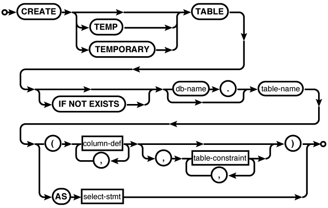
list all of the DDL commands (CREATE
TABLE, CREATE INDEX,
etc.) used to define the database. For a more complete list of all the
sqlite3 command-line options and
dot-commands, see Appendix A.
SQLite is designed to integrate into a wide variety of code bases on a broad range of platforms. This flexibility provides a great number of options, even for the most basic situations. While flexibility is usually a good thing, it can make for a lot of confusion when you’re first trying to figure things out.
If you’re just starting out, and all you need is a copy
of the sqlite3 shell, don’t get too
caught up in all the advanced build techniques. You can download one of the
precompiled executables or build
your own with the one-line commands provided in this chapter. That will get
you started.
As your needs evolve, you may need a more specific build
of sqlite3, or you may start to look at
integrating the SQLite library into your own application. At that point you
can try out different build techniques and see what best matches your needs
and build environment.
While the amalgamation is a somewhat unusual form for source distribution, it has proven itself to be quite useful and well suited for integrating SQLite into larger projects with the minimal amount of fuss. It is also the only officially supported source distribution format. It works well for the majority of projects.
This chapter provides an overview of the Structured Query Language, or SQL. Although sometimes pronounced “sequel,” the official pronunciation is to name each letter as “ess-cue-ell.” The SQL language is the main means of interacting with nearly all modern relational database systems. SQL provides commands to configure the tables, indexes, and other data structures within the database. SQL commands are also used to insert, update, and delete data records, as well as query those records to look up specific data values.
All interaction with a relational database is done through the SQL language. This is true when interactively typing commands or when using the programming API. In all cases, data is stored, modified, and retrieved through SQL commands. Many times, people look through the list of API calls, looking for functions that provide direct program access to the table or index data structures. Functions of this sort do not exist. The API is structured around preparing and issuing SQL commands to the database engine. If you want to query a table or insert a value using the API, you must create and execute the proper SQL command. If you want to do relational database programming, you must know SQL.
The goal of this chapter is to introduce you to all the major SQL commands and show some of the basic usage patterns. The first time you read through this chapter, don’t feel you need to absorb everything at once. Get an idea of what structures the database supports, and how they might be used, but don’t feel that you need to memorize the details of every last command.
For people just getting started, the most important commands are CREATE
TABLE, INSERT, and
SELECT. These will let you create a
table, insert some data into the table, and then query the data and display
it. Once you get comfortable with those commands, you can start to look at
the others in more depth. Feel free to refer back to this chapter, or the
command reference in Appendix C. The command reference
provides detailed descriptions of each command, including some of the more
advanced syntax that isn’t covered in this chapter.
Always remember that SQL is a command language. It
assumes you know what you’re doing. If you’re directly entering SQL commands
through the sqlite3 application, the
program will not stop and ask for confirmation before processing dangerous
or destructive commands. When entering commands by hand, it is always worth
pausing and looking back at what you’ve typed before you hit return.
If you are already reasonably familiar with the SQL language, it should be safe to skim this chapter. Much of the information here is on the SQL language in general, but there is some information about the specific dialect of SQL that SQLite recognizes. Again, Appendix C provides a reference to the specific SQL syntax used by SQLite.
Although the first official SQL specification was published in 1986 by the American National Standards Institute (ANSI), the language traces its roots back to the early 1970s and the pioneering relational database work that was being done at IBM. Current SQL standards are ratified and published by the International Standards Organization (ISO). Although a new standard is published every few years, the last significant set of changes to the core language can be traced to the SQL:1999 standard (also known as “SQL3”). Subsequent standards have mainly been concerned with storing and processing XML-based data. Overall, the evolution of SQL is firmly rooted in the practical aspects of database development, and in many cases new standards only serve to ratify and standardize syntax or features that have been present in commercial database products for some time.
The core of SQL is a declarative language. In a declarative language, you state what you want the results to be and allow the language processor to figure out how to deliver the desired results. Compare this to imperative languages, such as C, Java, Perl, or Python, where each step of a calculation or operation must be explicitly written out, leaving it up to the programmer to lead the program, step by step, to the correct conclusion.
The first SQL standards were specifically designed
to make the language approachable and usable by “non-computer
people”—at least by the 1980s definition of that term. This is one of
the reasons why SQL commands tend to have a somewhat English-like
syntax. Most SQL commands take the form
verb-subject. For example, CREATE (verb) TABLE (subject), DROP
INDEX, UPDATE
.table_name
The almost-English, declarative nature of SQL has both advantages and disadvantages. Declarative languages tend to be simpler (especially for nonprogrammers) to understand. Once you get used to the general structure of the commands, the use of English keywords can make the syntax easier to remember. The fixed command structure also makes it much easier for the database engine to optimize queries and return data more efficiently.
The predefined nature of declarative statements
can sometimes feel a bit limited, however—especially in a
command-based language like SQL, where individual, isolated commands
are constructed and issued one at a time. If you require a query that
doesn’t fit into the processing order defined by the SELECT command, you may find yourself
having to patch together nested queries or temporary tables. This is
especially true when the problem you’re trying to solve is inherently
nonrelational, and you’re forced to jump through extra hoops to
account for that.
Despite its oddities and somewhat organic evolution, SQL is a powerful language with a surprisingly broad ability to express complex operations. Once you wrap your head around what makes SQL tick, you can often find moderately simple solutions to even the most off-the-beaten-path problems. It can take some adjustment, however, especially if your primary experience is with imperative languages.
SQL’s biggest flaw is that formal standardization has almost always followed common implementations. Almost every database product (including SQLite) has custom extensions and enhancements to the core language that help differentiate it from other products, or expose features or control systems that are not covered by the core SQL standard. Often these enhancements are related to performance enhancements, and can be difficult to ignore.
While this less-strict approach to language purity has allowed SQL to grow and evolve in very practical ways, it means that “real world” SQL portability is not all that practical. If you strictly limit yourself to standardized SQL syntax, you can achieve a moderate degree of portability, but normally this comes at the cost of lower performance and less data integrity. Generally, applications will write to the specific SQL dialect they’re using and not worry about cross-database compatibility. If cross-database compatibility is important to a specific application, the normal approach is to develop a core list of SQL commands required by the application, with minor tweaks for each specific database product.
SQLite makes an effort to follow the SQL standards as much as possible. SQLite will also recognize and correctly parse a number of nonstandard syntax conventions used by other popular databases. This can help with the portability issues.
SQL is not without other issues, but considering its lineage, it is surprisingly well suited for the task at hand. Love it or hate it, it is the relational database language of choice, and it is likely to be with us for a long time.
Before getting into specific commands in SQL, it is worth looking at the general language structure. Like most languages, SQL has a fairly complete expression syntax that can be used to define command parameters. A more detailed description of the expression support can be found in Appendix D.
SQL consists of a number of different commands,
such as CREATE TABLE or INSERT. These commands are issued and
processed one at a time. Each command implements a different action or
feature of the database system.
Although it is customary to use all capital letters for SQL commands and keywords, SQL is a case-insensitive[1] language. All commands and keywords are case insensitive, as are identifiers (such as table names and column names).
Identifiers must be given as literals. If
necessary, identifiers can be enclosed in the standards compliant
double-quotes (" ") to allow the
inclusion of spaces or other nonstandard characters in an identifier.
SQLite also allows identifiers to be enclosed in square brackets ([ ]) or back
ticks (` `) for
compatibility with other popular database products. SQLite reserves
the use of any identifier that uses sqlite_ as a prefix.
SQL is whitespace insensitive, including line
breaks. Individual statements are separated by a semicolon. If you’re using an interactive application,
such as the sqlite3
command-line tool, then you’ll
need to use a semicolon to indicate the end of a statement. The
semicolon is not strictly required for single statements, however, as
it is properly a statement separator and not a statement terminator.
When passing SQL commands into the programming API, the semicolon is
not required unless you are passing more than one command statement
within a single string.
Single-line comments start with a double dash (--) and go
to the end of the line. SQL also supports multi-line comments using
the C comment syntax (/*
*/).
As with most languages, numeric literals are represented bare. Both integer (453) and real (rational) numbers
(43.23) are recognized, as is
exponent-style scientific notation (9.745e-6). In order to avoid ambiguities in the
parser, SQLite requires that the decimal point is always represented
as a period (.), regardless of the
current internationalization setting.
Text literals are enclosed in single quotes (' '). To represent a
string literal that includes a single quote character, use two single
quotes in a row (publisher =
'O''Reilly'). C-style
backslash escapes ( \'
) are not part of the SQL standard and are not supported by SQLite.
BLOB literals (binary data) can be represented as an x (or X) followed by a string literal of hexadecimal
characters (x'A554E59C').
Text literals use single quotes. Double quotes are reserved for identifiers (table names, columns, etc.). C-style backslash escapes are not part of the SQL standard.
SQL statements and expressions frequently contain lists. A comma is used as the list separator. SQL does not allow for a trailing comma following the last item of a list.
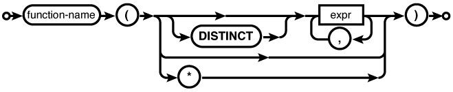
In general, expressions can be used any place a literal data value is allowed. Expressions can include both mathematical statements, as well as functions. Function-calling syntax is similar to most other computer languages, utilizing the name of the function, followed by a list of parameters enclosed in parentheses. Expressions can be grouped into subexpressions using parentheses.
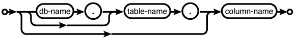
If an expression is evaluated in the context of a row (such as a filtering expression), the value of a row element can be extracted by naming the column. You may have to qualify the column name with a table name or alias. If you’re using cross-database queries, you may also have to specify which database you’re referring to. The syntax is:
[[database_name.]table_name.]column_name
If no database name is given, it is assumed you’re
referring to the main database on
the default connection. If the table name/alias is also omitted, the
system will make a best-guess using just the column name, but will
return an error if the name is ambiguous.
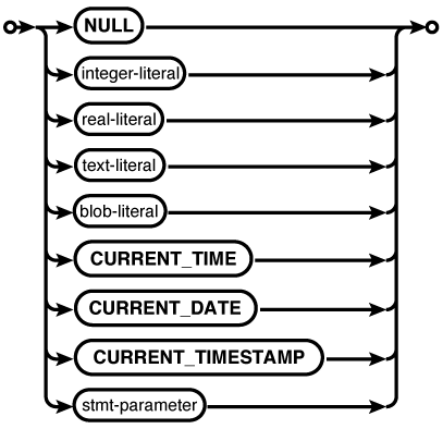
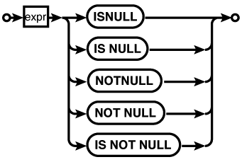
SQL allows any value to be assigned a NULL. NULL is not a value in itself (SQLite actually implements it as a unique valueless type), but is used as a marker or flag to represent unknown or missing data. The thought is that there are times when values for a specific row element may not be available or may not be applicable.
A NULL may not be a value, but it can be assigned
to data elements that normally have values, and can therefore show up
in expressions. The problem is that NULLs don’t interact well with
other values. If a NULL represents an unknown that might be any
possible value, how can we know if the expression NULL > 3 is true or
false?
To deal with this problem, SQL must employ a concept called three-valued logic. Three-valued logic is often abbreviated TVL or 3VL, and is more formally known as ternary logic. 3VL essentially adds an “unknown” state to the familiar true/false Boolean logic system.
Here are the truth tables for the 3VL
operators
NOT, AND, and OR:
3VL also dictates how comparisons work. For
example, any equality check (=)
involving a NULL will evaluate to NULL, including NULL = NULL. Remember that NULL is not
a value, it is a flag for the unknown, so the expression NULL = NULL is asking, “Does this
unknown equal that unknown?” The only practical answer is, “That is
unknown.” It might, but it might
not. Similar rules apply to greater-than, less-than, and other
comparisons.
You cannot use the equality operator
(=) to test for NULLs.
You must use the IS NULL
operator.
If you’re having trouble resolving an expression,
just remember that a NULL marks an unknown or unresolved value. This
is why the expression False AND
NULL is false, but True AND
NULL is NULL. In the case of the first expression, the
NULL can be replaced by either true or false without altering the
expression result. That isn’t true of the second expression, where the
outcome is unknown (in other words, NULL) because the output depends
on the unknown input.
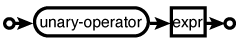
SQLite supports the following unary prefix operators:
- +
These adjust the sign of a
value. The “-” operator flips the sign of the value,
effectively multiplying it by -1.0. The “+” operator is
essentially a no-op, leaving a value with the same
sign it previously had. It does not make negative
values positive.
~
As in the C language, the “~” operator performs a
bit-wise inversion. This operator is not part of
the SQL standard.
NOT
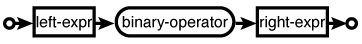
There are also a number of binary operators. They are listed here in descending precedence.
||
String concatenation. This is the only string concatenation operator recognized by the SQL standard. Many other database products allow “+” to be used for concatenation, but SQLite does not.
+ - * / %
Standard arithmetic operators for addition, subtraction, multiplication, division, and modulus (remainder).
| &
<< >>
The bitwise operators or, and, and shift-high/shift-low, as found in the C language. These operators are not part of the SQL standard.
< <=
=> >
Comparison test operators. Again, just as in the C language we have less-than, less-than or equal, greater-than or equal, and greater than. These operators are subject to SQL’s 3VL regarding NULLs.
= == !=
<>
Equality test operators. Both “=” and “==” will test for
equality, while both “!=” and “<>” test for inequality.
Being logic operators, these tests are subject to
SQL’s 3VL regarding NULLs. Specifically, value = NULL will always
return NULL.
IN LIKE GLOB MATCH
REGEXP
These five keywords are logic operators, returning, true, false, or NULL state. See Appendix D for more specifics on these operators.
AND OR
In addition to these basics, SQL supports a number of specific expression operations. For more information on these and any SQL-specific expressions, see Appendix D.
[1] Unless otherwise specified, case insensitivity only applies to ASCII characters. That is, characters represented by values less than 128.
SQL commands are divided into four major categories, or
languages. Each language defines a subset of
commands that serve a related purpose. The first language is the
Data Definition Language, or
DDL, which refers to commands that define the
structure of tables, views, indexes, and other data containers and objects
within the database. CREATE TABLE (used
to define a new table) and DROP VIEW
(used to delete a view) are examples of DDL commands.
The second category of commands is known as
Data Manipulation Language, or
DML. These are all of the commands that insert,
update, delete, and query actual data values from the data structures
defined by the DDL. INSERT (used to
insert new values into a table) and SELECT (used to query or look up data from tables) are
examples of DML commands.
Related to the DML and DDL is the Transaction Control Language, or
TCL. TCL commands can be used to control
transactions of DML and DDL commands. BEGIN (used to begin a multistatement transaction) and
COMMIT (used to end and accept a
transaction) are examples of TCL commands.
The last category is the Data Control Language, or
DCL. The main purpose of the DCL is to grant or
revoke access control. Much like file permissions, DCL commands are used to
allow (or deny) specific database users (or groups of users) permission to
utilize or access specific resources within a database. These permissions
can apply to both the DDL and the DML. DDL permissions might include the
ability to create a real or temporary table, while DML permissions might
include the ability to read, update, or delete the records of a specific
table. GRANT (used to assign a
permission) and REVOKE (used to delete an
existing permission) are the primary DCL commands.
SQLite supports the majority of standardized DDL, DML, and TCL commands but lacks any DCL commands. Because SQLite does not have user names or logins, it does not have any concept of assigned permissions. Rather, SQLite depends on datatype permissions to define who can open and access a database.
The DDL is used to define the structure of data containers and objects
within the database. The most common of these containers and objects are
tables, indexes, and views. As you’ll see, most objects are defined with a
variation of the CREATE command, such as
CREATE TABLE or CREATE VIEW. The DROP command is used to delete an existing object (and all
of the data it might contain). Examples include DROP TABLE or DROP
INDEX. Because the command syntax is so different, statements like
CREATE TABLE or CREATE INDEX are usually considered to be
separate commands, and not variations of a single CREATE command.
In a sense, the DDL commands are similar to C/C++ header files. DDL commands are used to define the structure, names, and types of the data containers within a database, just as a header file typically defines type definitions, structures, classes, and other data structures. DDL commands are typically used to set up and configure a brand new database before data is entered.
DDL commands define the basic structure of the database and are typically run when a new database is created.
DDL commands are often held in a script file, so that
the structure of the database can be easily recreated. Sometimes, especially
during development, you may need to recreate only part of the database. To
help support this, most CREATE commands
in SQLite have an optional IF NOT EXISTS
clause.
Normally, a CREATE
statement will return an error if an object with the requested name already
exists. If the optional IF NOT EXISTS
clause is present, then this error is suppressed and nothing is done, even
if the structure of the existing object and the new object are not
compatible. Similarly, most DROP
statements allow an optional IF EXISTS
clause that silently ignores any request to delete an object that isn’t
there.
In the examples that follow, the IF EXISTS and IF
NOT EXISTS command variations are not explicitly called out.
Please see the SQLite command reference in Appendix C for
the full details on the complete syntax supported by SQLite.
The most common DDL command is CREATE
TABLE. No data values can be stored in a database
until a table is defined to hold that data. At the bare minimum, the
CREATE TABLE command defines
the table name, plus the name of each column. Most of the time you’ll
want to define a type for each column as well, although types are
optional when using SQLite. Optional constraints, conditions, and
default values can also be assigned to each column. Table-level
constraints can also be assigned, if they involve multiple
columns.
In some large RDBMS systems, CREATE TABLE can be quite complex,
defining all kinds of storage options and configurations. SQLite’s
version of CREATE TABLE is somewhat
simpler, but there are still a great many options available. For full
explanation of the command, see CREATE TABLE
in Appendix C.
The most basic syntax for CREATE
TABLE looks something like this:
CREATE TABLEtable_name(column_namecolumn_type, [...] );
A table name must be provided to identify the new table. After that, there is just a simple list of column names and their types. Table names come from a global namespace of all identifiers, including the names of tables, views, and indexes.
Clear and concise identifier names are important. Like the database design itself, some careful thought should be put into the table name, trying to pin down the precise meaning of the data it contains. Much the same could be said of column names. Table names and column names tend to be referenced frequently in queries, so there is some desire to keep them as brief as possible while still keeping their purpose clear.
Most databases use strong, static column typing. This means that the elements of a column can only hold values compatible with the column’s defined type. SQLite utilizes a dynamic typing technique known as manifest typing. For each row value, manifest typing records the value’s type along with the value data. This allows nearly any element of any row to hold almost any type of value.
In the strictest sense, SQLite supports only five concrete datatypes. These are known as storage classes, and represent the different ways SQLite might choose to store data on disk. Every value has one of these five native storage classes:
A NULL is considered its own distinct type. A
NULL type does not hold a value. Literal NULLs are
represented by the keyword NULL.
A signed integer number. Integer values are variable length, being 1, 2, 3, 4, 6, or 8 bytes in length, depending on the minimum size required to hold the specific value. Integer have a range of −9,223,372,036,854,775,808 to +9,223,372,036,854,775,807, or roughly 19 digits. Literal integers are represented by any bare series of numeric digits (without commas) that does not include a decimal point or exponent.
A floating-point number, stored as an 8-byte value in the processor’s native format. For nearly all modern processors, this is an IEEE 754 double-precision number. Literal floating-point numbers are represented by any bare series of numeric digits that include a decimal point or exponent.
A variable-length string, stored using the database encoding (UTF-8, UTF-16BE, or UTF-16LE). Literal text values are represented using character strings in single quotes.
A length of raw bytes,
copied exactly as provided. Literal
BLOBs are represented as hexadecimal text strings
preceded by an x. For example, the notation x'1234ABCD' represents a
4-byte BLOB. BLOB stands for Binary Large
OBject.
SQLite text and BLOB values are always variable length. The maximum size of a text or BLOB value is limited by a compile-time directive. The default limit is exactly one billion bytes, or slightly less than a full gigabyte. The maximum value for this directive is two gigabytes.
Since the elements of most columns can hold
any value type, the “type” of a column is a somewhat misleading
concept. Rather than being an absolute type, as in most
databases, an SQLite column type (as defined in CREATE TABLE) becomes more of a
suggestion than a hard and fast rule. This is known as
a
type affinity, and essentially represents
a desired category of type. Each type affinity has specific
rules about what types of values it can store, and how different
values will be converted when stored in that column. Generally,
a type affinity will cause a conversion or migration of types
only if it can be done without losing data or precision.
Each table column must have one of five type affinities:
A column with a text affinity will only store values of type NULL, text, or BLOB. If you attempt to store a value with a numeric type (float or integer) it will be converted into a text representation before being stored as a text value type.
A column with a numeric affinity will store any of the five types. Values with integer and float types, along with NULL and BLOB types, are stored without conversion. Any time a value with a text type is stored, an attempt is made to convert the value to a numeric type (integer or float). Assuming the conversion works, the value is stored in an appropriate numeric type. If the conversion fails, the text value is stored without any type of conversion.
A column with an integer affinity works essentially the same as a numeric affinity. The only difference is that any value with a float type that lacks a fractional component will be converted into an integer type.
A column with a floating-point affinity also works essentially the same as a numeric affinity. The only difference is that most values with integer types are converted into floating-point values and stored as a float type.
A column with a none affinity has no preference over storage class. Each value is stored as the type provided, with no attempt to convert anything.
Since type affinities are not part of the SQL standard, SQLite has a series of rules that attempt to map traditional column types to the most logical type affinity. The type affinity of a column is determined by the declared type of the column, according to the following rules (substring matches are case-insensitive):
If no column type was given, then the column is given the none affinity.
If the column type contains the substring “INT,” then the column is given the integer affinity.
If the column type contains any of the substrings “CHAR,” “CLOB,” or “TEXT,” then the column is given the text affinity.
If the column type contains the substring “BLOB,” then the column is given the none affinity.
If the column type contains any of the substrings “REAL,” “FLOA,” or “DOUB,” then it is given the float affinity.
If no match is found, the column is assigned the numeric affinity.
As implied by the first rule, the column
type is completely optional. SQLite will allow you to create a
table by simply naming the columns, such as CREATE TABLE t ( i, j, k);.
You’ll also notice that there isn’t any specific list of column
types that are recognized. You can use any column type you want,
even making up your own names.
This might sound a bit fast and loose for a typing system, but it works out quite well. By keying off specific substrings, rather than trying to define specific types, SQLite is able to handle SQL statements (and their database-specific types) from just about any database, all while doing a pretty good job of mapping the types to an appropriate affinity. About the only type you need to be careful of is “floating point.” The “int” in “point” will trigger rule 2 before the “floa” in “floating” will get to rule 5, and the column affinity will end up being integer.
In addition to column names and types, a table definition can also
impose constraints on specific columns or sets of columns. A
more complete view of the CREATE
TABLE command looks something like this:
CREATE TABLEtable_name(column_namecolumn_typecolumn_constraints..., [... ,]table_constraints, [...] );
Here we see that each individual column can have additional, optional constraints and modifiers placed on it. Column constraints only affect the column for which they are defined, while table constraints can be used to define a constraint across one or more columns. Constraints that involve two or more columns must be defined as table constraints.
Column constraints can be used to define a
custom sort order (COLLATE
).
Collations determine how text values are sorted. In addition to
user-defined collations, SQLite includes a collation_nameNOCASE collation that ignores
case when sorting.
A default value (DEFAULT ) can
also be assigned. Nearly all columns have a default of NULL. You
can use the valueDEFAULT column
constraint to set a different default value. The default can
either be a literal or an expression. Expressions must be placed
in parentheses.
To help with date and time defaults, SQLite
also includes three special keywords that may be used as a default value:
CURRENT_TIME, CURRENT_DATE, and CURRENT_TIMESTAMP. These will
record the UTC time, date, or date and time, respectively, when
a new row is inserted. See Date and Time Features for
more information on date and time functions.
Column constraints can also impose limits on
a column, like denying NULL (NOT
NULL) or requiring a unique value for each row
(UNIQUE). Remember that
a NULL is not considered a value, so UNIQUE does not imply NOT NULL, nor does UNIQUE imply only a single NULL is allowed. If
you want to keep NULL assignments out of a UNIQUE column, you need to
explicitly mark the column NOT
NULL.
Column values can also be subjected to
arbitrary user-defined constraints before they are assigned
(CHECK (
).
Some types of constraints also allow you to specify the action
to be taken in situations when the constraint would be violated.
See CREATE TABLE and UPDATE in Appendix C
for more specific details.expression )
When multiple column constraints are used on a single column, the constraints are listed one after another without commas. Some examples:
CREATE TABLE parts
(
part_id INTEGER PRIMARY KEY,
stock INTEGER DEFAULT 0 NOT NULL,
desc TEXT CHECK( desc != '' ) -- empty strings not allowed
);In order to enforce a UNIQUE column constraint, a
unique index will be automatically created over that column. A
different index will be created for each column (or set of
columns) marked UNIQUE. There
is some expense in maintaining an index, so be aware that
enforcing a UNIQUE column
constraint can have performance considerations.
In addition to these other constraints, a
single column (or set of columns) can be designated as the
PRIMARY KEY. Each table
can have only one primary key. Primary keys must be unique, so
designating a column as PRIMARY
KEY implies the UNIQUE constraint as well, and will result in
an automatic unique index being created. If a column is marked
both UNIQUE and PRIMARY KEY, only one index will
be created.
In SQLite, PRIMARY
KEY does not imply NOT
NULL. This is in contradiction to the SQL
standard and is considered a bug, but the behavior is so
long-standing that there are concerns about fixing it and
breaking existing applications. As a result, it is always a good
idea to explicitly mark at least one column from each PRIMARY KEY as NOT NULL.
There are also some good design reasons for
defining a primary key, which will be discussed in Tables and Keys, but the only significant,
concrete thing that comes out of defining a PRIMARY KEY is the automatic
unique index. There are also some minor syntax shortcuts.
If, however, the primary key column has a
type that is designated as INTEGER (and very specifically INTEGER), then that column
becomes the table’s “root” column.
SQLite must have some column that can be
used to index the base storage for the table. In a sense, that
column acts as the master index that is used to store the table
itself. Like many other database systems, SQLite will silently
create a hidden ROWID column
for this purpose. Different database systems use different names
so, in an effort to maintain compatibility, SQLite will
recognize the names ROWID,
OID, or _ROWID_ to reference the root
column. Normally ROWID
columns are not returned (even for column wildcards), nor are
their values included in dump files.
If a table includes an INTEGER PRIMARY KEY column, then
that column becomes an alias for the automatic ROWID column. You can still
reference the column by any of the ROWID names, but you can also reference the
column by its “real” user-defined name. Unlike PRIMARY KEY by itself, INTEGER PRIMARY KEY columns do
have an automatic NOT NULL
constraint associated with them. They are also strictly typed to
only accept integer values.
There are two significant advantages of
INTEGER PRIMARY KEY
columns. First, because the column aliases the table’s root
ROWID column, there is
no need for a secondary index. The table itself acts as the
index, providing efficient lookups without the maintenance costs
of an external index.
Second, INTEGER
PRIMARY KEY columns can automatically provide
unique default values. When you insert a row without an explicit
value for the ROWID (or
ROWID alias) column,
SQLite will automatically choose a value that is one greater
than the largest existing value in the column. This provides an
easy means to automatically generate unique keys. If the maximum
value is reached, the database will randomly try other values,
looking for an unused key.
INTEGER PRIMARY
KEY columns can optionally be marked as AUTOINCREMENT. In that case, the
automatically generated ID values will constantly increase,
preventing the reuse of an ID value from a previously deleted
row. If the maximum value is reached, insertions with automatic
INTEGER PRIMARY KEY
values are no longer possible. This is unlikely, however, as the
INTEGER PRIMARY KEY
type domain is large enough to allow 1,000 inserts per second
for almost 300 million years.
When using either automatic or AUTOINCREMENT values, it is always possible to
insert an explicit ROWID (or
ROWID alias) value.
Other than the INTEGER PRIMARY
KEY designation, SQLite offers no other type of
automatic sequence feature.
In addition to a PRIMARY KEY,
columns can also be marked as a FOREIGN
KEY. These columns reference rows in another
(foreign) table. Foreign keys can be used to create links
between rows in different tables. See Tables and Keys for details.
Table definitions can also include table-level constraints. In general, table constraints and column constraints work the same way. Table-level constraints still operate on individual rows. The main difference is that using the table constraint syntax, you can apply the constraint to a group of columns rather than just a single column. It is perfectly legal to define a table constraint with only one column, effectively defining a column constraint. Multicolumn constraints are sometimes known as compound constraints.
At the table level, SQLite supports the
UNIQUE, CHECK, and PRIMARY KEY constraints. The
check constraint is very similar, requiring only an expression
(CHECK
().
Both the expression)UNIQUE and PRIMARY KEY constraints, when
given as a table constraint, require a list of columns (e.g.,
UNIQUE
(, column_name,
[...])PRIMARY KEY
(). As with column constraints, any
table-level column_name,
[...])UNIQUE or
PRIMARY KEY (which
implies UNIQUE) constraint
will automatically create a unique index over the appropriate
columns.
Table constraints that are applied to
multiple columns use the set of columns as a group. For example,
when UNIQUE or PRIMARY KEY is applied across
more than one column, each individual column is allowed to have
duplicate values. The constraint only prevents the set of values
across the designated columns from being replicated. If you
wanted each individual column to also be UNIQUE, you’d need to add the
appropriate constraints to the individual columns.
Consider a table that contains records of all the rooms in a multibuilding campus:
CREATE TABLE rooms
(
room_number INTEGER NOT NULL,
building_number INTEGER NOT NULL,
[...,]
PRIMARY KEY( room_number, building_number )
);Clearly we need to allow for more than one
room with the number 101. We also need to allow for more than
one room in building 103. But there should only be one room 101
in building 103, so we apply the constraint across both columns.
In this example, we’ve chosen to make these columns into a
compound primary key, since the building number and room number
combine to quintessentially define a specific room. Depending on
the design of the rest of the database, it might have been
equally valid to define a simple UNIQUE constraint across these two columns, and
designated an arbitrary room_id column as the primary key.
You can also create a table from the output of a query. This is a slightly
different
CREATE TABLE syntax that
creates a new table and preloads it with data, all in one
command:
CREATE [TEMP] TABLEtable_nameAS SELECTquery_statement;
Using this form, you do not designate the
number of columns or their names or types. Rather, the query
statement is run and the output is used to define the column
names and preload the new table with data. With this syntax,
there is no way to designate column constraints or modifiers.
Any result column that is a direct column reference will inherit
the column’s affinity, but and all columns are given a NONE affinity. The query
statement consists of a SELECT command. More information on SELECT can be found in Chapter 5.
Tables created in this manner are not
dynamically updated—the query command is run only once when the
table is created. Once the data is entered into the new table,
it remains unaltered until you change it. If you need a
table-like object that can dynamically update itself, use a
VIEW (Views).
This example shows the optional
TEMP keyword (the full word
TEMPORARY can also be
used) in CREATE TEMP TABLE.
This modifier can be used on any variation of CREATE TABLE, but is frequently
used in conjunction with the ...AS
SELECT... variation shown here. Temporary tables
have two specific features. First, temporary tables can only be
seen by the database connection that created them. This allows
the simultaneous re-use of table names without any worry of
conflict between different clients. Second, all associated
temporary tables are automatically dropped and deleted whenever
a database connection is closed.
Generally speaking, CREATE TABLE...AS SELECT is not the best choice
for creating standard
tables. If you need to copy data from an old table into a new
table, a better choice is to use CREATE
TABLE to define an empty table with all of the
appropriate column modifiers and table constraints. You can then
bulk copy all the data into the new table using a variation of
the INSERT command that
allows for query statements. See INSERT for details.
SQLite supports a limited version of the ALTER TABLE command. Currently, there are only
two operations supported by ALTER
TABLE: add column and
rename. The add column variant allows
you to add new columns to an existing table. It cannot remove
them. New columns are always added to the end of the column
list. Several other restrictions apply.
If you need to make a more significant change while preserving as much data as possible, you can use the rename variant to rename the existing table, create a new table under the original name, and then copy the data from the old table to the new table. The old table can then be safely dropped.
For full details, see ALTER TABLE in Appendix C.
The CREATE
TABLE command is used to create tables and DROP TABLE is used to delete them. The DROP TABLE command deletes a
table and all of the data it contains. The table definition is
also removed from the database system catalogs.
The DROP
TABLE command is very simple. The only argument
is the name of the table you wish to drop:
DROP TABLE table_name;In addition to deleting the table, DROP TABLE will also drop any
indexes associated with the table. Both automatically created
indexes (such as those used to enforce a UNIQUE constraint) as well as
manually created indexes will be dropped.
Virtual tables can be used to connect any data source to SQLite, including
other databases. A virtual table is created with the CREATE VIRTUAL TABLE command.
Although very similar to CREATE
TABLE, there are important differences. For
example, virtual tables cannot be made temporary, nor do they
allow for an IF NOT EXISTS
clause. To drop a virtual table, you use the normal DROP TABLE command.
For more information on virtual tables,
including the full syntax for CREATE VIRTUAL
TABLE, see Chapter 10.
Views provide a way to package queries into a predefined object. Once
created, views act more or less like read-only tables. Just like
tables, new views can be marked as TEMP, with the same result. The basic syntax of
the
CREATE VIEW command is:
CREATE [TEMP] VIEWview_nameAS SELECTquery_statement
The CREATE VIEW
syntax is almost identical to the CREATE
TABLE...AS SELECT command. This is because both
commands serve a similar purpose, with one important difference. The
result of a CREATE TABLE command is
a new table that contains a full copy of the data. The SELECT statement is run exactly once
and the output of the query is stored in the newly defined table. Once
created, the table will hold its own, independent copy of the
data.
A view, on the other hand, is fully dynamic. Every
time the view is referenced or queried, the underlying SELECT statement is run to regenerate
the view. This means the data seen in a view automatically updates as
the data changes in the underlying tables. In a sense, views are
almost like named queries.
Views are commonly used in one of two ways. First, they can be used to package up commonly used queries into a more convenient form. This is especially true if the query is complex and prone to error. By creating a view, you can be sure to get the same query each time.
Views are also commonly used to create user-friendly versions of standard tables. A common example are tables with date and time records. Normally, any time or date value is recorded in Coordinated Universal Time, or UTC. UTC is a more proper format for dates and times because it is unambiguous and time-zone independent. Unfortunately, it can also be a bit confusing if you’re several time zones away. It is often useful to create a view that mimics the base table, but converts all the times and dates from UTC into the local time zone. This way the data in the original tables remains unchanged, but the presentation is in units that are more user-friendly.
Views are dropped with the
DROP VIEW command:
DROP VIEW view_name;Dropping a view will not have any effect on the tables it references.
Indexes (or indices) are a means to optimize database lookups by pre-sorting and indexing one or more columns of a table. Ideally, this allows specific rows in a table to be found without having to scan every row in the table. In this fashion, indexes can provide a large performance boost to some types of queries. Indexes are not free, however, requiring updates with each modification to a table as well as additional storage space. There are even some situations when an index will cause a drop in performance. See Indexes for more information on when it makes sense to use an index.
The basic syntax for creating an index specifies the name of the new index, as well as the table and column names that are indexed. Indexes are always associated with one (and only one) table, but they can include one or more columns from that table:
CREATE [UNIQUE] INDEXindex_nameONtable_name(column_name[, ...] );
Normally indexes allow duplicate values. The
optional
UNIQUE keyword indicates that
duplicate entries are not allowed, and any attempt to insert or update
a table with a nonunique value will cause an error. For unique indexes
that reference more than one column, all the columns must match for an
entry to be considered duplicate. As discussed with CREATE TABLE, NULL isn’t considered a
value, so a UNIQUE index will not
prevent one or more NULLs. If you want to prevent NULLs, you must
indicate NOT NULL in the original
table definition.
Each index is tied to a specific table, but they
all share a common namespace. Although you can name an index anything
you like, it is standard practice to name an index with a standard
prefix (such as idx_), and then
include the table name and possibly the names of the columns included
in the index. For example:
CREATE INDEX idx_employees_name ON employees ( name );
This makes for long index names but, unlike table or view names, you typically only reference an index’s name when you create it and when you drop it.
As with all the DROP commands, the DROP INDEX
command is very simple, and requires only the name of the index that
is being dropped:
DROP INDEX index_name;Dropping an index will remove the index from the database, but will leave the associated table intact.
As described earlier, the CREATE TABLE command will automatically create unique
indexes to enforce a UNIQUE or
PRIMARY KEY constraint. All
automatic indexes will start with an sqlite_ prefix. Because these indexes are required to
enforce the table definition, they cannot be manually dropped with the
DROP INDEX command. Dropping
the automatic indexes would alter the table behavior as defined by the
original CREATE TABLE
command.
Conversely, if you have manually defined a
UNIQUE index, dropping that
index will allow the database to insert or update redundant data. Be
careful when auditing indexes and remember that not all indexes are
created for performance reasons.
The Data Manipulation Language is all about getting user data in and out of the database. After all the data structures and other database objects have been created with DDL commands, DML commands can be used to load those data structures full of useful data.
The DML supported by SQLite falls into two basic
categories. The first category consists of the “update” commands, which
includes the actual UPDATE command, as
well as the INSERT and DELETE commands. As you might guess, these
commands are used to update (or modify), insert, and delete the rows of a
table. All of these commands alter the stored data in some way. The update
commands are the primary means of managing all the data within a
database.
The second category consists of the “query” commands,
which are used to extract data from the database. Actually, there is only
one query command: SELECT. The SELECT command not only prints returned
values, but provides a great number of options to combine different tables
and rows and otherwise manipulate data before returning the final
result.
SELECT is,
unquestionably, the most complex SQL command. It is also, arguably, the most
important SQL command. This chapter will only cover the very basics of
SELECT, and then we will spend the
next chapter going through all of its parts, bit by bit. To address the full
command syntax in detail, SELECT gets a
whole chapter to itself (Chapter 5).
There are three commands used for adding,
modifying, and removing data from the database. INSERT adds new rows, UPDATE modifies existing rows, and
DELETE removes rows. These
three commands are used to maintain all of the actual data values
within the database. All three update commands operate at a row level,
adding, altering, or removing the specified rows. Although all three
commands are capable of acting on multiple rows, each command can only
directly act upon rows contained within a single table.
The INSERT command is used to create new rows in the specified table.
There are two meaningful versions of the command. The first
version uses a VALUES clause
to specify a list of values to insert:
INSERT INTOtable_name(column_name[, ...]) VALUES (new_value[, ...]);
A table name is provided, along with a list of columns and a list of values. Both lists must have the same number of items. A single new row is created and each value is recorded into its respective column. The columns can be listed in any order, just as long as the list of columns and the list of values line up correctly. Any columns that are not listed will receive their default values:
INSERT INTO parts ( name, stock, status ) VALUES ( 'Widget', 17, 'IN STOCK' );
In this example, we attempt to insert a new row into a “parts” table. Note the use of single quotes for text literals.
Technically, the list of column names is
optional. If no explicit list of columns is provided, the
INSERT command will
attempt to pair up values with the table’s full list of
columns:
INSERT INTOtable_nameVALUES (new_value[, ...]);
The trick with this format is that the
number and order of values must exactly match the number and
order of columns in the table definition. That means it is
impossible to use default values, even on INTEGER PRIMARY KEY columns.
More often than not, this is not actually desirable. This format
is also harder to maintain within application source code, since
it must be meticulously updated if the table format changes. In
general, it is recommended that you always explicitly list out
the columns in an INSERT
statement.
When bulk importing data, it is common to
loop over data sets, calling INSERT over and over. Processing these
statements one at a time can be fairly slow, since each command
will update both the table and any relevant indexes, and then
make sure the data is fully written out to physical disk before
(finally!) starting the next INSERT. This is a fairly lengthly process,
since it requires physical I/O.
To speed up bulk inserts, it is common to
wrap groups of 1,000 to 10,000 INSERT statements into a single transaction.
Grouping the statement together will substantially increase the
overall speed of the inserts by delaying the physical I/O until
the end of the transaction. See Transaction Control Language
for more information on transactions.
The second version of INSERT allows you to define
values by using a query statement. This is very similar to the
CREATE TABLE...AS
SELECT command, although the table must already
exist. This is the only version of INSERT that can insert more than one row with a
single command:
INSERT INTOtable_name(column_name, [...]) SELECTquery_statement;
This type of INSERT is most commonly used to bulk copy data
from one table to another. This is a common operation when you
need to update the definition of a table, but you don’t want to
lose all the data that already exists in the database. The old
table is renamed, the new table is defined, and the data is
copied from the old table into the new table using an INSERT INTO...SELECT command.
This form can also be used to populate temporary tables or copy
data from one attached database to another.
As with the VALUES version of INSERT, the column list is technically optional
but, for all the same reasons, it is still recommended that you
provide an explicit column list.
All versions of the INSERT command also support an optional
conflict resolution clause. This conflict clause determines what
should be done if the results of the INSERT would violate a database constraint. The
most common example is INSERT OR
REPLACE, which comes into play when the INSERT would, as executed, cause
a UNIQUE constraint
violation. If the REPLACE
conflict resolution is present, any existing row that would
cause a UNIQUE constraint
violation is first deleted, and then the INSERT is allowed to continue.
This specific usage pattern is so common that the whole INSERT OR REPLACE phrase can be
replaced by just REPLACE. For
example, REPLACE INTO
.table_name...
See INSERT and UPDATE in Appendix C for more information on the details of conflict resolution.
The UPDATE command is used to assign new values to one or more columns of
existing rows in a table. The command can update more than one
row, but all of the rows must be part of the same table. The
basic syntax is:
UPDATEtable_nameSETcolumn_name=new_value[, ...] WHEREexpression
The command requires a table name followed
by a list of column name/value pairs that should be assigned.
Which rows are updated is determined by a conditional expression
that is tested against each row of the table. The most common
usage pattern uses the expression to check for equality on some
unique column, such as a PRIMARY
KEY column.
If no WHERE condition is given, the UPDATE command will
attempt to update the designated columns in
every row of a table.
It is not considered an error if the
WHERE expression
evaluates to false for every row in the table, resulting in no
actual updates.
Here is a more specific example:
-- Update the price and stock of part_id 454: UPDATE parts SET price = 4.25, stock = 75 WHERE part_id = 454;
This example assumes that the table parts has at least three
columns: price, stock, and part_id. The database will find
each row with a part_id of
454. In this case, it can be assumed that part_id is a PRIMARY KEY column, so only one
row will be updated. The price and stock columns of that row are then assigned new
values.
The full syntax for UPDATE can be found at UPDATE in Appendix C.
As you might guess, the DELETE command is used to delete or remove one or more rows from a
single table. The rows are completely deleted from the
table:
DELETE FROMtable_nameWHEREexpression;
The command requires only a table name and a
conditional expression to pick out rows. The WHERE expression is used to
select specific rows to delete, just as it is used in the
UPDATE command.
If no WHERE condition is given, the DELETE command will
attempt to delete every row of a
table.
As with UPDATE, it is not considered an error if the
WHERE expression
evaluates to false for every row in the table, resulting in no
actual deletions.
-- Delete the row with rowid 385: DELETE FROM parts WHERE part_id = 385; -- Delete all rows with a rowid greater than or equal to 43 -- and less than or equal to 246: DELETE FROM parts WHERE part_id >= 43 AND part_id <= 246;
These examples assume we have a table named
parts that contains at
least one unique column named part_id.
As noted, if no WHERE clause is given, the DELETE command will attempt to
delete every row in a table. SQLite optimizes this specific
case, truncating the full table, rather than processing each
individual row. Truncating the table is much faster than
deleting each individual row, but truncation bypasses the
individual row processing. If you wish to process each row as it
is deleted, provide a WHERE
clause that always evaluates to true:
DELETE FROM parts WHERE 1; -- delete all rows, force per-row processing
The existence of the WHERE clause will prevent the
truncation, allowing each row to be processed in turn.
The final DML command to cover is the SELECT
command. SELECT is used to extract
or return values from the database. Almost any time you want to
extract or return some kind of value, you’ll need to use the SELECT command. Generally, the
returned values are derived from the contents of the database, but
SELECT can also be used to
return the value of simple expressions. This is a great way to test
out expressions, for example:
sqlite> SELECT 1+1, 5*32, 'abc'||'def', 1>2;
1+1 5*32 'abc' || 'def' 1>2
---------- ---------- -------------- ----------
2 160 abcdef 0 SELECT is a
read-only command, and will not modify the database (unless the
SELECT is embedded in a
different command, such as a CREATE
TABLE...AS SELECT or an INSERT INTO...SELECT).
Without question, SELECT is the most complex SQL command, both in terms
of syntax as well as function. The SELECT syntax tries to represent a generic framework
that is capable of expressing a great many different types of queries.
While it is somewhat successful at this, there are areas where
SELECT has traded away
simplicity for more flexibility. As a result, SELECT has a large number of optional clauses, each
with its own set of options and formats.
Understanding how to mix and match these optional
clauses to get the result you’re looking for can take some time. While
the most basic syntax can be shown with a good set of examples, to
really wrap your head around SELECT, it is best to understand how it actually works and
what it is trying to accomplish.
Because SELECT
can be so complex, and because SELECT is an extremely important command, we will
spend the whole next chapter looking very closely at SELECT and each of its clauses. There
will be some discussion about what is going on behind the scenes, to
provide more insight into how to read and write complex
queries.
For now, we’ll just give you a taste. That should
provide enough information to play around with the other commands in
this chapter. The most basic form of SELECT is:
SELECToutput_listFROMinput_tableWHERErow_filter;
The output list is a list of expressions that
should be evaluated and returned for each resulting row. Most
commonly, this is simply a list of columns. The output list can also
include a wildcard (*) that
indicates all known columns should be returned.
The FROM clause
defines the source of the table data. The next chapter will show
how tables can be linked and joined, but for now we’ll stick with
querying one table at a time.
The WHERE
clause is a conditional filtering expression that is applied to each
row. It is essentially the same as the WHERE clause in the UPDATE and DELETE
commands. Those rows that evaluate to true will be part of the result,
while the other rows will be filtered out.
sqlite>CREATE TABLE tbl ( a, b, c, id INTEGER PRIMARY KEY );sqlite>INSERT INTO tbl ( a, b, c ) VALUES ( 10, 10, 10 );sqlite>INSERT INTO tbl ( a, b, c ) VALUES ( 11, 15, 20 );sqlite>INSERT INTO tbl ( a, b, c ) VALUES ( 12, 20, 30 );
We can return the whole table like this:
sqlite> SELECT * FROM tbl;
a b c id
---------- ---------- ---------- ----------
10 10 10 1
11 15 20 2
12 20 30 3 We can also just return specific columns:
sqlite> SELECT a, c FROM tbl;
a c
---------- ----------
10 10
11 20
12 30 sqlite> SELECT * FROM tbl WHERE id = 2;
a b c id
---------- ---------- ---------- ----------
11 15 20 2 For more specifics, see Chapter 5 and SELECT in Appendix C.
The Transaction Control Language is used in conjunction with the Data Manipulation Language to control the processing and exposure of changes. Transactions are a fundamental part of how relational databases protect the integrity and reliability of the data they hold. Transactions are automatically used on all DDL and DML commands.
A transaction is used to group together a series of low-level changes into a single, logical update. A transaction can be anything from updating a single value to a complex, multistep procedure that might end up inserting several rows into a number of different tables.
The classic transaction example is a database that holds account numbers and balances. If you want to transfer a balance from one account to another, that is a simple two-step process: subtract an amount from one account balance and then add the same amount to the other account balance. That process needs to be done as a single logical unit of change, and should not be broken apart. Both steps should either succeed completely, resulting in the balance being correctly transferred, or both steps should fail completely, resulting in both accounts being left unchanged. Any other outcome, where one step succeeds and the other fails, is not acceptable.
Typically a transaction is opened, or started. As individual data manipulation commands are issued, they become part of the transaction. When the logical procedure has finished, the transaction can be committed, which applies all of the changes to the permanent database record. If, for any reason, the commit fails, the transaction is rolled back, removing all traces of the changes. A transaction can also be manually rolled back.
The standard for reliable, robust transactions is the ACID test. ACID stands for Atomic, Consistent, Isolated, and Durable. Any transaction system worth using must possess these qualities.
A transaction should be atomic, in the sense that the change cannot be broken down into smaller pieces. When a transaction is committed to the database, the entire transaction must be applied or the entire transaction must not be applied. It should be impossible for only part of a transaction to be applied.
A transaction should also keep the database consistent. A typical database has a number of rules and limits that help ensure the stored data is correct and consistent with the design of the database. Assuming a database starts in a consistent state, applying a transaction must keep the database consistent. This is important, because the database is allowed to (and is often required to) become inconsistent while the transaction is open. For example, while transferring funds, there is a moment between the subtraction from one account and the addition to another account that the total amount of funds represented in the database is altered and may become inconsistent with a recorded total. This is acceptable, as long as the transaction, as a whole, is consistent when it is committed.
An open transaction must also be isolated from other clients. When a client opens a transaction and starts to issue individual change commands, the results of those commands are visible to the client. Those changes should not, however, be visible to any other system accessing the database, nor should they be integrated into the permanent database record until the entire transaction is committed. Conversely, changes committed by other clients after the transaction was started should not be visible to this transaction. Isolation is required for transactions to be atomic and consistent. If other clients could see half-applied transactions, the transactions could not claim to be atomic in nature, nor would they preserve the consistency of the database, as seen by other clients.
Last of all, a transaction must be durable. If the transaction is successfully committed, it must have become a permanent and irreversible part of the database record. Once a success status is returned, it should not matter if the process is killed, the system loses power, or the database filesystem disappears—upon restart, the committed changes should be present in the database. Conversely, if the system loses power before a transaction is committed, then upon restart the changes made within the transaction should not be present.
Most people think that the atomic nature of transactions is their most important quality, but all four aspects must work together to ensure the overall integrity of the database. Durability, especially, is often overlooked. SQLite tries extremely hard to guarantee that if a transaction is successfully committed, those changes are actually physically written to permanent storage and are there to stay. Compare this to traditional filesystem operations, where writes might go into an operating system file cache. Updates may sit in the cache anywhere from a few seconds to a few minutes before finally being spooled off to storage. Even then, it is possible for the data to wait around in device buffers before finally being committed to physical storage. While this type of buffering can increase efficiency, it means that a normal application really has no idea when its data is safely committed to permanent storage.
Power failures and disappearing filesystems may seem like rare occurrences, but that’s not really the point. Databases are designed to deal with absolutes, especially when it comes to reliability. Besides, having a filesystem disappear is not that radical of an idea when you consider the prevalence of flash drives and USB thumb drives. Disappearing media and power failures are even more commonplace when you consider the number of SQLite databases that are found on battery-operated, handheld devices such as mobile phones and media players. The use of transactions is even more important on devices like this, since it is nearly impossible to run data recovery tools in that type of environment. These types of devices must be extremely robust and, no matter what the user does (including yanking out flash drives at inconvenient times), the system must stay consistent and reliable. Use of a transactional system can provide that kind of reliability.
Transactions are not just for writing data. Opening a transaction for an extended read-only operation is sometimes useful if you need to gather data with multiple queries. Having the transaction open keeps your view of the database consistent, ensuring that the data doesn’t change between queries. That is useful if, for example, you use one query to gather a bunch of record IDs, and then issue a series of queries against each ID value. Wrapping all the queries in a transaction guarantees all of the queries see the same set of data.
Normally, SQLite is in autocommit mode. This means that SQLite will automatically start a transaction for each command, process the command, and (assuming no errors were generated) automatically commit the transaction. This process is transparent to the user, but it is important to realize that even individually entered commands are processed within a transaction, even if no TCL commands are used.
The autocommit mode can be disabled by explicitly
opening a transaction. The BEGIN
command is used to start or open a transaction. Once an explicit
transaction has been opened, it will remain open until it is committed
or rolled back. The keyword
TRANSACTION is optional:
BEGIN [ DEFERRED | IMMEDIATE | EXCLUSIVE ] [TRANSACTION]
The optional keywords
DEFERRED, IMMEDIATE, or EXCLUSIVE are specific to SQLite and control how the
required read/write locks are acquired. If only one client is
accessing the database at a time, the locking mode is largely
irrelevant. When more than one client may be accessing the database,
the locking mode defines how to balance peer access with ensured
success of the transaction.
By default, all transactions (including autocommit
transactions) use the DEFERRED
mode. Under this mode, none of the database locks are acquired until
they are required. This is the most “neighborly” mode and allows other
clients to continue accessing and using the database until the
transaction has no other choice but to lock them out. This allows
other clients to continue using the database, but if the locks are not
available when the transaction requires them, the transaction will
fail and may need to be rolled back and restarted.
BEGIN IMMEDIATE
attempts to acquire a reserved lock immediately. If it
succeeds, it guarantees the write locks will be available to the
transaction when they are needed, but still allows other clients to
continue to access the database for read-only operations. The EXCLUSIVE mode attempts to lock out
all other clients, including read-only
clients. Although the IMMEDIATE and
EXCLUSIVE modes are more
restrictive to other clients, the advantage is that they will fail
immediately if the required locks are not available, rather than after
you’ve issued your DDL or DML commands.
Once a transaction is open, you can continue to
issue other SQL commands, including both DML and DDL commands. You can
think of the changes resulting from these commands as “proposed”
changes. The changes are only visible to the local client and have not
been fully and permanently applied to the database. If the client
process is killed or the server loses power in the middle of an open
transaction, the transaction and any proposed changes it has will be
lost, but the rest of the database will remain intact and consistent.
It is not until the transaction is closed that the proposed changes
are committed to the database and made “real.” The COMMIT command is used to close out a transaction and commit the changes
to the database. You can also use the alias
END. As with BEGIN, the TRANSACTION keyword is optional.
COMMIT [TRANSACTION] END [TRANSACTION]
Once a COMMIT
has successfully returned, all the proposed changes are fully
committed to the database and become visible to other clients. At that
point, if the system loses power or the client process is killed, the
changes will remain safely in the database.
Things don’t always go right, however. Rather than committing the proposed changes, the transaction can be manually rolled back, effectively canceling the transaction and all of the changes it contains. Rolling back a set of proposed changes is useful if an error is encountered. This might be a database error, such as running out of disk space half-way through inserting a series of related records, or it might be an application logic error, such as trying to assign an invoice to an order that doesn’t exist. In such cases, it usually doesn’t make sense to continue with the transaction, nor does it make sense to leave inconsistent data in the database. Pretty much the only choice is to back out and try again.
To cancel the transaction and roll back all the
proposed changes, you can use the ROLLBACK command. Again, the keyword TRANSACTION is
optional:
ROLLBACK [TRANSACTION]
ROLLBACK will
undo and revert all the proposed changes made by the current
transaction and then close the transaction. It does not necessarily
return the database to its prior state, as other clients may have been
making changes in parallel. A ROLLBACK only cancels the proposed changes made by
this client within the current transaction.
Both COMMIT and
ROLLBACK will end the current
transaction, putting SQLite back into autocommit mode.
In addition to ACID-compliant transactions, SQLite also supports save-points. Save-points allow you to mark specific points in the transaction. You can then accept or rollback to individual save-points without having to commit or rollback an entire transaction. Unlike transactions, you can have more than one save-point active at the same time. Save-points are sometimes called nested transactions.
Save-points are generally used in conjunction with large, multistep transactions, where some of the steps or sub-procedures require rollback ability. Save-points allow a transaction to proceed and (if required) roll back one step at a time. They also allow an application to explore different avenues, attempting one procedure, and if that doesn’t work, trying another, without having to roll back the entire transaction to start over. In a sense, save-points can be thought of as “undo” markers in SQL command stream.
You can create a save-point with the
SAVEPOINT command. Since multiple
save-points can be defined, you must provide a name to identify the
save-point:
SAVEPOINT savepoint_nameSave-points act as a stack. Whenever you create a new one, it is put at the top of the stack. Save-point identifiers do not need to be unique. If the same save-point identifier is used more than once, the one nearest to the top of the stack is used.
To release a save-point and accept all of the
proposed changes made since the save-point was set, use the
RELEASE command:
RELEASE [SAVEPOINT] savepoint_nameThe RELEASE
command does not commit any changes to disk. Rather, it flattens all
of the changes in the save-point stack into the layer below the named
save-point. The save-point is then removed. Any save-points contained
by the named save-point are automatically released.
To cancel a set of commands and undo everything
back to where a save-point was set, use the
ROLLBACK TO command:
ROLLBACK [TRANSACTION] TO [SAVEPOINT] savepoint_nameUnlike a transaction ROLLBACK, a save-point ROLLBACK TO does not close out and eliminate the
save-point. ROLLBACK TO rolls back
and cancels any changes issued since the save-point was established,
but leaves the transaction state exactly as it was
after the SAVEPOINT command was issued.
Consider the following series of SQL statements. The indentation is used to show the save-point stack:
CREATE TABLE t (i);
BEGIN;
INSERT INTO t (i) VALUES 1;
SAVEPOINT aaa;
INSERT INTO t (i) VALUES 2;
SAVEPOINT bbb;
INSERT INTO t (i) VALUES 3;At this point, if the command ROLLBACK TO bbb is issued, the state
of the database would be as if the following commands were
entered:
CREATE TABLE t (i);
BEGIN;
INSERT INTO t (i) VALUES 1;
SAVEPOINT aaa;
INSERT INTO t (i) VALUES 2;
SAVEPOINT bbb;Again, notice that rolling back to save-point
bbb still leaves the
save-point in place. Any new commands will be associated with SAVEPOINT bbb. For example:
CREATE TABLE t (i);
BEGIN;
INSERT INTO t (i) VALUES 1;
SAVEPOINT aaa;
INSERT INTO t (i) VALUES 2;
SAVEPOINT bbb;
DELETE FROM t WHERE i=1;Continuing, if the command RELEASE aaa was issued, we would get
the equivalent of:
CREATE TABLE t (i); BEGIN; INSERT INTO t (i) VALUES 1; INSERT INTO t (i) VALUES 2; DELETE FROM t WHERE i=1;
In this case, the proposed changes from both the
aaa and the enclosed bbb save-points were released and
merged outward. The transaction is still open, however, and a COMMIT would
still be required to make the proposed changes permanent.
Even if you have open save-points, you can still issue transaction commands. If the enclosing transaction is committed, all outstanding save-points will automatically be released and then committed. If the transaction is rolled back, all the save-points are rolled back.
If the SAVEPOINT command is issued when SQLite is in
autocommit mode—that is, outside of a transaction—then a standard
autocommit BEGIN DEFERRED
TRANSACTION will be started. However, unlike with most
commands, the autocommit transaction will not automatically commit
after the SAVEPOINT command
returns, leaving the system inside an open transaction. The automatic
transaction will remain active until the original save-point is
released, or the outer transaction is either explicitly committed or
rolled back. This is the only situation when a save-point RELEASE will have a direct effect on
the enclosing transaction. As with other save-points, if an autocommit
save-point is rolled back, the transaction will remain open and the
original save-point will be open, but empty.
Many relational database systems, including SQLite, keep system state data in a series of
data structures known as
system catalogs. All of the SQLite system catalogs
start with the prefix sqlite_. Although
many of these catalogs contain internal data, they can be queried, using
SELECT, just as if they were
standard tables. Most system catalogs are read-only. If you encounter an
unknown database and you’re not sure what’s in it, examining the system
catalogs is a good place to start.
All nontemporary SQLite databases have an
sqlite_master catalog. This is the master
record of all database objects. If any of the tables has a populated
AUTOINCREMENT column, the database
will also have an sqlite_sequence
catalog. This catalog is used to keep track of the next valid sequence value
(for more information on AUTOINCREMENT,
see Primary keys). If the SQL command ANALYZE has been used, it will also generate
one or more sqlite_stat tables, such as
#sqlite_stat1 and sqlite_stat2. These tables hold various
statistics about the values and distributions in various indexes, and are
used to help the query optimizer pick the more efficient query solution. For
more information, see ANALYZE in Appendix C.
The most important of these system catalogs is the sqlite_master table. This catalog contains information on
all the objects within a database, including the SQL used to define them.
The sqlite_master table has five
columns:
| Column name | Column type | Meaning |
type
| Text | Type of database object |
name
| Text | Identifier name of object |
tbl_name
| Text | Name of associated table |
rootpage
| Integer | Internal use only |
sql
| Text | SQL used to define object |
The type column can be table (including virtual tables), index, view, or trigger. The
name column gives the name of the
object itself, while the tbl_name column
gives the name of the table or view the object is associated with. For
tables and views, the tbl_name is just a
copy of the name column. The final
sql column holds a full copy of the
original SQL command used to define the object, such as a CREATE TABLE or CREATE TRIGGER command.
Temporary databases do not have an sqlite_master system catalog. Rather, they have an sqlite_temp_master table instead.
This is a long chapter packed with a huge amount of information. Even if you’re familiar with a number of traditional programming languages, the declarative nature of SQL often takes time to wrap your head around. One of the best ways to learn SQL is to simply experiment. SQLite makes it easy to open up a test database, create some tables, and try things out. If you’re having problems understanding the details of a command, be sure to look it up in Appendix C. In addition to more detailed descriptions, Appendix C contains detailed syntax diagrams .
If you wish to make a deeper study into SQL, there are literally hundreds of books to choose from. O’Reilly alone publishes a dozen or so titles just on the SQL language. While there are some differences between the SQL supported by SQLite and other major database systems, SQLite follows the standard fairly closely. Most of the time, SQLite deviates from the standard, it does so in an attempt to support common notations or usage in other popular database products. If you’re working on wrapping you’re head around some of the higher level concepts, or basic query structures, a tutorial or book written for just about any database product is likely to help. There might be a small bit of tweaking to get the queries to run under SQLite, but the changes are usually minimal.
Popular O’Reilly books covering the SQL language include Learning SQL (Beaulieu), SQL in a Nutshell (Kline, Kline, Hunt), and the SQL Cookbook (Molinaro). More advanced discussions can be found in The Art of SQL (Faroult, Robson). Popular reference books also include SQL For Smarties (Celko, Morgan Kaufmann) and Introduction to SQL (van der Lans, Addison Wesley). These two are large, but very complete. There is also The SQL Guide to SQLite (van der Lans, lulu.com), which takes a much deeper look at the SQL dialect specifically used by SQLite.
There are also thousands of websites and online tutorials, communities, and forums, including the SQLite mailing lists, where you can often get insightful answers to intelligent questions.
Before trying too much, be sure to read the next
chapter. The next chapter is devoted to the SELECT command. In addition to covering the syntax of the
command, it dives a bit deeper into what is going on behind the scenes. That
foundation knowledge should make it much easier to break down and understand
complex queries. It should also make it much easier to write them.
The SELECT command is
used to extract data from the database. Any time you want to query or
return user data stored in a database table, you’ll need to use the SELECT
command.
In terms of both syntax and functionality, SELECT is the most complex SQL command. In most
applications, it is also one of the most frequently used commands. If you want to
get the most out of your database (and your database designs), you’ll need a solid
understanding of how to properly use SELECT.
Generally, the returned values are derived from the contents
of the database, but SELECT can also be used to
return the value of simple expressions. SELECT
is a read-only command, and will not modify the database (unless the SELECT is embedded in a different command, such as
INSERT INTO...SELECT).
The main SQL data structure is the table. Tables are used for both storage and for
data manipulation. We’ve seen how to define tables with the CREATE TABLE command, but let’s look at some
of the details.
A table consists of a heading and a body. The heading defines the name and type (in SQLite, the affinity) of each column. Column names must be unique within the table. The heading also defines the order of the columns, which is fixed as part of the table definition.
The table body contains all of the rows. Each row consists of one data element for each column. All of the rows in a table must have the same number of data elements, one for each column. Each element can hold exactly one data value (or a NULL).
SQL tables are allowed to hold duplicate rows. Tables can contain multiple rows where every user-defined column has an equivalent corresponding value. Duplicate rows are normally undesirable in practice, but they are allowed.
The rows in an SQL table are unordered. When a table is displayed or written down, it will have some inherent ordering, but conceptually tables have no ordering. The order of insertion has no meaning to the database.
A very common mistake is to assume a given query will always return rows in the same order. Unless you’ve specifically asked a query to sort the returned rows in a specific order, there is no guarantee the rows will continue to come back in the same order. Don’t let your application code become dependent on the natural ordering of an unordered query. A different version of SQLite may optimize the query differently, resulting in a different row ordering. Even something as simple as adding or dropping an index can alter the row ordering of an unsorted result.
To verify your code is making no assumptions about row
order, you can turn on PRAGMA
reverse_unordered_selects. This will cause SQLite to reverse the natural row ordering of
any SELECT statement that does not have
an explicit order (an ORDER BY clause).
See reverse_unordered_selects in Appendix F for more details.
The SELECT syntax
tries to represent a generic framework that is capable of expressing
many different types of queries. To achieve this, SELECT has a large number of optional clauses, each with
its own set of options and formats.
The most general format of a standalone SQLite SELECT statement looks like this:
SELECT [DISTINCT]select_headingFROMsource_tablesWHEREfilter_expressionGROUP BYgrouping_expressionsHAVINGfilter_expressionORDER BYordering_expressionsLIMITcountOFFSETcount
Every SELECT command
must have a select heading, which defines the returned values. Each
additional line (FROM, WHERE, GROUP
BY, etc.) represents an optional clause.
Each clause represents a step in the SELECT pipeline. Conceptually, the result of
a SELECT statement is calculated by
generating a working table, and then passing that table through the
pipeline. Each step takes the working table as input, performs a specific
operation or manipulation, and passes the modified table on to the next
step. Manipulations operate the whole working table, similar to vector or
matrix operations.
Practically, the database engine takes a few shortcuts and makes plenty of optimizations when processing a query, but the end result should always match what you would get from independently going through each step, one at a time.
The clauses in a SELECT statement are not evaluated in the same order they
are written. Rather, their evaluation order looks something like
this:
Designates one or more source tables and combines them together into one large working table.
Groups sets of rows in the working table based off similar values.
Defines the result set columns and (if applicable) grouping aggregates.
Filters specific rows out of the grouped table. Requires a
GROUP BY.
Skips over rows at the beginning of the result set.
Requires a LIMIT.
No matter how large or complex a SELECT statement may be, they all follow
this basic pattern. To understand how any query works, break it down and
look at each individual step. Make sure you understand what the working
table looks like before each step, how that step manipulates and modifies
the table, and what the working table looks like when it is passed to the
next step.
The FROM clause
takes one or more source tables from the database and
combines them into one large table. Source tables are usually named
tables from the database, but they can also be views or subqueries
(see Subqueries for more details on
subqueries).
Tables are combined using the JOIN operator. Each JOIN combines two tables into a larger
table. Three or more tables can be joined together by stringing a
series of JOIN operators together.
JOIN operators are evaluated
left-to-right, but there are several different types of joins, and not
all of them are commutative or associative. This makes the ordering
and grouping very important. If necessary, parentheses can be used to
group the joins correctly.
Joins are the most important and most powerful database operator. Joins are the only way to bring together information stored in different tables. As we’ll see in the next chapter, nearly all of database design theory assumes the user is comfortable with joins. If you can master joins, you’ll be well on your way to mastering relational databases.
SQL defines three major types of joins: the
CROSS JOIN, the INNER JOIN, and the OUTER JOIN.
A CROSS
JOIN matches every row of the first table with every row of the
second table. If the input tables have x
and y columns, respectively, the resulting
table will have x+y columns. If the input
tables have n and m
rows, respectively, the resulting table will have
n·m rows. In mathematics, a CROSS JOIN is known as a
Cartesian product.
The syntax for a CROSS JOIN is quite simple:
SELECT ... FROM t1 CROSS JOIN t2 ...
Figure 5-1 shows
how a CROSS JOIN is
calculated.
Because CROSS
JOINs have the potential to generate extremely
large tables, care must be taken to only use them when
appropriate.
An INNER
JOIN is very similar to a CROSS
JOIN, but it has a built-in condition that is
used to limit the number of rows in the resulting table. The
conditional is normally used to pair up or match rows from the
two source tables. An INNER
JOIN without any type of conditional expression
(or one that always evaluates to true) will result in a CROSS JOIN. If the input tables
have x and y columns,
respectively, the resulting table will have no more than
x+y columns (in some cases, it can
have fewer). If the input tables have n and
m rows, respectively, the resulting
table can have anywhere from zero to n·m
rows, depending on the condition. An INNER JOIN is the most common type of join, and
is the default type of join. This makes the INNER keyword optional.
There are three primary ways to specify the
conditional. The first is with an ON expression. This provides a simple
expression that is evaluated for each potential row. Only those
rows that evaluate to true are actually joined. A JOIN...ON looks like
this:
SELECT ... FROM t1 JOIN t2 ON conditional_expression ...An example of this is shown in Figure 5-2.
If the input tables have
C and D columns,
respectively, a JOIN...ON
will always result in C+D columns.
The conditional expression can be used to
test for anything, but the most common type of expression tests
for equality between similar columns in both tables. For
example, in a business employee database, there is likely to be
an employee table that
contains (among other things) a name column and an eid column (employee ID number). Any other
table that needs to associate rows to a specific employee will
also have an eid column that
acts as a pointer or reference to the correct employee. This
relationship makes it very common to have queries with ON expressions similar
to:
SELECT ... FROM employee JOIN resource ON employee.eid = resource.eid ...
This query will result in an output table
where the rows from the resource table are correctly matched to their
corresponding rows in the employee table.
This JOIN
has two issues. First, that ON condition is a lot to type out for something
so common. Second, the resulting table will have two eid columns, but for any given
row, the values of those two columns will always be identical.
To avoid redundancy and keep the phrasing shorter, inner join
conditions can be declared with a USING expression. This expression specifies a
list of one or more columns:
SELECT ... FROM t1 JOIN t2 USING ( col1 ,... ) ...
Queries from the employee database would now look something like this:
SELECT ... FROM employee JOIN resource USING ( eid ) ...
To appear in a USING condition, the column name must exist in
both tables. For each listed column name, the USING
condition will test for equality between the pairs
of columns. The resulting table will have only one instance of
each listed column.
If this wasn’t concise enough, SQL provides an additional
shortcut. A
NATURAL JOIN is similar to a
JOIN...USING, only it
automatically tests for equality between the values of every
column that exists in both tables:
SELECT ... FROM t1 NATURAL JOIN t2 ...
If the input tables have
x and y columns,
respectively, a JOIN...USING
or a NATURAL JOIN will result
in anywhere from max(x,y) to
x+y columns.
Assuming eid is the only column identifier to appear in
both the employee and
resource table, our
business query becomes extremely simple:
SELECT ... FROM employee NATURAL JOIN resource ...
NATURAL
JOINs are convenient, as they are very concise,
and allow changes to the key structure of various tables without
having to update all of the corresponding queries. They can also
be a tad dangerous unless you follow some discipline in naming
your columns. Because none of the columns are explicitly named,
there is no error checking in the sanity of the join. For
example, if no matching columns are found, the JOIN will automatically (and
without warning) degrade to a CROSS
JOIN, just like any other INNER JOIN. Similarly, if two
columns accidentally end up with the same name, a NATURAL JOIN will automatically
include them in the join condition, if you wanted it or
not.
The OUTER
JOIN is an extension of the INNER
JOIN. The SQL standard defines three types of
OUTER JOINs: LEFT, RIGHT, and FULL. Currently, SQLite only supports the
LEFT OUTER JOIN.
OUTER
JOINs have a conditional that is identical to
INNER JOINs, expressed
using an ON, USING, or NATURAL keyword. The initial
results table is calculated the same way. Once the primary
JOIN is calculated, an
OUTER join will take
any unjoined rows from one or both tables, pad them out with
NULLs, and append them to the resulting table. In the case of a
LEFT OUTER JOIN, this
is done with any unmatched rows from the first table (the table
that appears to the left of the word JOIN).
Figure 5-3 shows
an example of a LEFT OUTER
JOIN.
The result of a LEFT OUTER JOIN will contain at least one
instance of every row from the lefthand table. If the input
tables have x and y
columns, respectively, the resulting table will have no more
than x+y columns (the exact number depends
on which conditional is used). If the input tables have
n and m rows,
respectively, the resulting table can have anywhere from
n to n·m
rows.
Because they include unmatched rows,
OUTER JOINs are often
specifically used to search for unresolved or “dangling”
rows.
Because the JOIN operator combines the columns of different tables into one,
larger table, there may be cases when the resulting working
table has multiple columns with the same name. To avoid
ambiguity, any part of the SELECT statement can qualify any column
reference with a source-table name. However, there are some
cases when this is still not enough. For example, there are some
situations when you need to join a table to itself, resulting in
the working table having two instances of the same source-table.
Not only does this make every column name ambiguous, it makes it
impossible to distinguish them using the source-table name.
Another problem is with subqueries, as they don’t have concrete
source-table names.
To avoid ambiguity within the SELECT statement, any instance
of a source-table, view, or subquery can be assigned an alias.
This is done with the AS
keyword. For example, in the cause of a self-join, we can assign
a unique alias for each instance of the same table:
SELECT ... FROM x AS x1 JOIN x AS x2 ON x1.col1 = x2.col2 ...
Or, in the case of a subquery:
SELECT ... FROM ( SELECT ... ) AS sub ...
Technically, the AS keyword
is optional, and each source-table name can simply
be followed with an
alias name. This can be quite confusing, however, so it is
recommended you use
the AS keyword.
If any of the subquery columns conflict with
a column from a standard source table, you can now use the
sub qualifier as a
table name. For example, sub.col1.
Once a table alias has been assigned, the original source-table name becomes invalid and cannot be used as a column qualifier. You must use the alias instead.
The WHERE
clause is used to filter rows from the working table
generated by the FROM clause. It is
very similar to the WHERE clause
found in the UPDATE and DELETE commands. An expression is
provided that is evaluated for each row. Any row that causes the
expression to evaluate to false or NULL is discarded. The resulting
table will have the same number of columns as the original table, but
may have fewer rows. It is not considered an error if the WHERE clause eliminates every row in
the working table. Figure 5-4 shows how the
WHERE clause works.
Some WHERE clauses can get quite
complex, resulting in a long series of AND operators used to join sub-expressions together.
Most filter for a specific row, however, searching for a specific key
value.
The GROUP BY
clause is used to collapse, or “flatten,” groups of rows. Groups can be
counted, averaged, or otherwise aggregated together. If you need to
perform any kind of inter-row operation that requires data from more
than one row, chances are you’ll need a GROUP
BY.
The GROUP BY
clause provides a list of grouping expressions and optional
collations. Very often the expressions are simple column references,
but they can be arbitrary expressions. The syntax looks like
this:
GROUP BYgrouping_expression[COLLATEcollation_name] [,...]
The grouping process has two steps. First, the
GROUP BY expression list is
used to arrange table rows into different groups. Once the groups are
defined, the SELECT header
(discussed in the next section) defines how those groups are flattened
down into a single row. The resulting table will have one row for each
group.
To split up the working table into groups, the list of expressions is evaluated across each row of the table. All of the rows that produce equivalent values are grouped together. An optional collation can be given with each expression. If the grouping expression involves text values, the collation is used to determine which values are equivalent. For more information on collations, see ORDER BY Clause.
Figure 5-5 shows how
the rows are grouped together with the GROUP
BY clause.
Once grouped together, each collection of rows is
collapsed into a single row. This is typically done using aggregate
functions that are defined in the SELECT heading, which is described in the next
section, on page .
Because it is common to GROUP BY using expressions that are defined in the
SELECT header, it is possible
to simply reference SELECT heading
expressions in the GROUP BY
expression list. If a GROUP BY
expression is given as a literal integer, that number is used as a
column index in the result table defined by the SELECT header. Indexes start at one
with the leftmost column. A GROUP
BY expression can also reference a result column
alias. Result column aliases are explained in the next section.
The SELECT
header is used to define the format and content of the final result table.
Any column you want to appear in the final results table must be
defined by an expression in the SELECT header. The SELECT heading is the only required step in the
SELECT command
pipeline.
The format of the header is fairly simple, consisting of a list of expressions. Each expression is evaluated in the context of each row, producing the final results table. Very often the expressions are simple column references, but they can be any arbitrary expression involving column references, literal values, or SQL functions. To generate the final query result, the list of expressions is evaluated once for each row in the working table.
Additionally, you can provide a column name
using the AS
keyword:
SELECTexpression[AScolumn_name] [,...]
Don’t confuse the AS keyword used in the SELECT header with the one used in the FROM clause. The SELECT header uses the AS keyword to assign a column name to
one of the output columns, while the FROM clauses uses the AS keyword to assign a source-table alias.
Providing an output column name is optional, but
recommended. The column name assigned to a results table is not
strictly defined unless the user provides an AS column alias. If your application searches for a
specific column name in the query results, be sure to assign a known
name using AS. Assigning a column
name will also allow other parts of the SELECT statement to reference an output column by
name. Steps in the SELECT pipeline
that are processed before the SELECT header, such as the WHERE and GROUP BY
clause, can also reference output columns by name, just as long as the
column expression does not contain an aggregate function.
If there is no working table (no FROM clause), the expression list is
evaluated a single time, producing a single row. This row is then used
as the working table. This is useful to test and evaluate standalone
expressions.
Although the SELECT header appears to filter columns from the
working table, much like the WHERE
clause filters rows, this isn’t exactly correct. All of the columns
from the original working table are still available to clauses that
are processed after the SELECT
header. For example, it is possible to sort the results (via ORDER BY, which is processed after the
SELECT header) using a column
that doesn’t appear in the query output.
It would be more accurate to say that the SELECT header tags specific columns
for output. Not until the whole SELECT pipeline has been processed and the results
are ready to be returned, are the unused columns stripped out. Figure 5-6 illustrates this point.
In addition to the standard expressions, SELECT supports two wildcards. A simple asterisk (*) will cause
every user-defined column from every source table in the FROM clause to be output. You can also
target a specific table (or table alias) using the format table_name.*
Be aware that the SELECT wildcards will not return any automatically
generated ROWID columns. To return
both the ROWID and the user-defined
columns, simply ask for them both:
SELECT ROWID, * FROM table;Wildcards do include any user-defined INTEGER PRIMARY KEY column that have
replaced the standard ROWID column.
See Primary keys for more information about how
ROWID and INTEGER PRIMARY KEY columns
interact.
In addition to determining the columns of the
query result, the SELECT header
determines how row-groups (produced by the GROUP BY clause) are flattened into a single row.
This is done using
aggregate functions. An aggregate function
takes a column expression as input and aggregates, or combines, all of
the column values from the rows of a group and produces a single
output value. Common aggregate functions include count(), min(), max(), and
avg(). Appendix E provides a full list of all the built-in
aggregate
functions.
Any column or expression that is not passed
through an aggregate function will assume whatever value was contained
in the last row of the group. However, because SQL tables are
unordered, and because the SELECT
header is processed before the ORDER
BY clause, we don’t really know which row is “last.”
This means the values for any unaggregated output will be taken from
some essentially random row in the group. Figure 5-7 shows how
this works.
In some cases, picking the value from a random row
is not a bad thing. For example, if a SELECT header expression is also used as a GROUP BY expression, then we know that
column has an equivalent value in every row of a group. No matter
which row you choose, you will always get the same value.
Where you can run into trouble is when the
SELECT header uses column
references that were not part of the GROUP
BY clause, nor were they passed through aggregate
functions. In those cases there is no deterministic way to figure out
what the output value will be. To avoid this, when using a GROUP BY clause, SELECT header expressions should only
use column references as aggregate function inputs, or the header
expressions should match those used in the GROUP BY clause.
Here are some examples. In this case all of the expressions are bare column references to help make things clear:
SELECT col1, sum( col2 ) FROM tbl GROUP BY col1; -- well formed
This is a well formed statement. The GROUP BY clause shows that the rows
are being grouped based off the values in col1. That makes it safe for col1 to appear in the SELECT header, since every row in a particular group
will have an equivalent value in col1. The SELECT
header also references col2, but it
is fed into an aggregate function. The aggregate function will take
all of the col2 values from
different rows in the group and produce a logical answer—in this case,
a numerical summation.
The result of this statement will be two columns.
The first column will have one row for each unique value from col1. Each row of the second column
will have the sum of all the values in col2 that are associated with the col1 value listed in the first result
column. More detailed examples can be found at the end of the
chapter.
This next statement is not well formed:
SELECT col1, col2 FROM tbl GROUP BY col1; -- NOT well formed
As before, the rows are grouped based off the
value in col1, which makes it safe
for col1 to appear in the SELECT header. The column col2 appears bare, however, and not as
an aggregate parameter. When this statement is run, the second return
column will contain random values from the original col2 column.
Although every row within a group should have an equivalent value in a
column or expression that was used as a grouping key, that doesn’t
always mean the values are the exact same. If a collation such as
NOCASE was used, different
values (such as 'ABC' and 'abc') are considered equivalent. In
these cases, there is no way to know the specific value that will be
returned from a SELECT header. For
example:
CREATE TABLE tbl ( t ); INSERT INTO tbl VALUES ( 'ABC' ); INSERT INTO tbl VALUES ( 'abc' ); SELECT t FROM tbl GROUP BY t COLLATE NOCASE;
This query will only return one row, but there is no way to know which specific value will be returned.
Finally, if the SELECT header contains an aggregate function, but the
SELECT statement has no
GROUP BY clause, the entire
working table is treated as a single group. Since flattened groups
always return one row, this will cause the query to return only one
row—even if the working table contained no rows.
Functionally, the
HAVING clause is identical to the
WHERE clause. The HAVING clause consists of a filter
expression that is evaluated for each row of the working table. Any
row that evaluates to false or NULL is filtered out and removed. The
resulting table will have the same number of columns, but may have
fewer rows.
The main difference between the WHERE clause and the HAVING clause is where they appear in
the SELECT pipeline. The HAVING clause is processed after the
GROUP BY and SELECT clauses, allowing HAVING to filter rows based off the
results of any GROUP BY aggregate.
HAVING clauses can even have
their own aggregates, allowing them to filter on aggregate results
that are not part of the SELECT
header.
HAVING clauses
should only contain filter expressions that depend on the GROUP BY output. All other filtering
should be done in the WHERE
clause.
Both the HAVING
and WHERE clauses can reference
result column names defined in the SELECT header with the AS keyword. The main difference is that the WHERE clause can only reference
expressions that do not contain aggregate functions, while the
HAVING clause can reference
any result column.
The DISTINCT
keyword will scan the result set and eliminate any duplicate rows.
This ensures the returned rows constitute a proper set. Only the
columns and values specified in the SELECT header are considered when determining if a
row is a duplicate or not. This is one of the few cases when NULLs are
considered to have “equality,” and will be eliminated.
Because SELECT
DISTINCT must compare every row against every other
row, it is an expensive operation. In a well-designed database, it is
also rarely required. Therefore, its usage is somewhat unusual.
The ORDER BY
clause is used to sort, or order, the rows of the results table. A
list of one or more sort expressions is provided. The first expression
is used to sort the table. The second expression is used to sort any
equivalent rows from the first sort, and so on. Each expression can be
sorted in ascending or descending order.
The basic format of the ORDER BY clause looks like this:
ORDER BYexpression[COLLATEcollation_name] [ASC|DESC] [,...]
The expression is evaluated for each row. Very
often the expression is a simple column reference, but it can be any
expression. The resulting value is then compared against those values
generated by other rows. If given, the named collation is used to sort
the values. A collation defines a specific sorting order for text
values. The
ASC or DESC keywords can be used to force the sort in an
ascending or descending order. By default, values are sorted in an
ascending order using the default collation.
An ORDER BY
expression can utilize any source column, including those that do not
appear in the query result. Like GROUP
BY, if an ORDER BY
expression consists of a literal integer, it is assumed to be a column
index. Column indexes start on the left with 1, so the phrase ORDER BY 2 will sort the results table
by its second column.
Because SQLite allows different datatypes to be stored in the same column, sorting can get a bit more interesting. When a mixed-type column is sorted, NULLs will be sorted to the top. Next, integer and real values will be mixed together in proper numeric order. The numbers will be followed by text values, with BLOB values at the end. There will be no attempt to convert types. For example, a text value holding a string representation of a number will be sorted in with the other text values, and not with the numeric values.
In the case of numeric values, the natural sort
order is well defined. Text values are sorted by the active collation,
while BLOB values are always sorted using the BINARY collation. SQLite comes with three built-in
collation functions. You can also use the API to define your own
collation functions. The three built-in collations are:
BINARY
Text values are sorted according
to the semantics of the POSIX memcmp() call. The
encoding of a text value is not
taken into account, essentially treating it as a
large binary string. BLOB values are always sorted
with this collation. This is the default
collation.
NOCASE
Same as BINARY, only ASCII uppercase characters
are converted to lowercase before the
comparison is done. The case-conversion is strictly
done on 7-bit ASCII values. The normal SQLite
distribution does not support UTF-aware
collations.
RTRIM
Same as BINARY, only trailing (righthand)
whitespace is ignored.
While ORDER BY
is extremely useful, it should only be used when it is actually
needed—especially with
very large result tables. Although SQLite can sometimes make use of an
index to calculate the query results in order, in many cases SQLite
must first calculate the entire result set and then sort it, before
rows are returned. In that case, the intermediate results table must
be held in memory or on disk until it is fully computed and can then
be sorted.
Overall, there are plenty of situations where
ORDER BY is justified, if not
required. Just be aware there can be some significant costs involved
in its use, and you shouldn’t get in the habit of tacking it on to
every query “just because.”
The LIMIT and
OFFSET clauses allow you to extract a specific subset of rows from the
final results table. LIMIT defines
the maximum number of rows that will be returned, while OFFSET defines the number of rows to
skip before returning the first row. If no OFFSET is provided, the LIMIT is applied to the top of the table. If a
negative LIMIT is provided, the
LIMIT is removed and will
return the whole table.
There are three ways to define a LIMIT and OFFSET:
LIMITlimit_countLIMITlimit_countOFFSEToffset_countLIMIToffset_count,limit_count
Note that if both a limit and offset are given using the third format, the order of the numbers is reversed.
Here are some examples. Notice that the OFFSET value defines how many rows are
skipped, not the position of the first row:
LIMIT 10 -- returns the first 10 rows (rows 1 - 10) LIMIT 10 OFFSET 3 -- returns rows 4 - 13 LIMIT 3 OFFSET 20 -- returns rows 21 - 23 LIMIT 3, 20 -- returns rows 4 - 23 (different from above!)
Although it is not strictly required, you usually
want to define an ORDER BY if
you’re using a LIMIT. Without an
ORDER BY, there is no
well-defined order to the result, making the limit and offset somewhat
meaningless.
Beyond the basic SELECT syntax, there are a few advanced techniques for
expressing more complex queries.
The SELECT
command provides a great deal of flexibility, but there are times
when a single SELECT command cannot
fully express a query. To help with these situations, SQL supports
subqueries. A subquery is nothing more
than a SELECT statement that is
embedded in another SELECT
statement. Subqueries are also known as sub-selects.
Subqueries are most commonly found in the FROM clause, where they act as a
computed source table. This type of subquery can return any number of
rows or columns, and is similar to creating a view or running the
query, recording the results into a temporary table, and then
referencing that table in the main query. The main advantage of using
an in-line subquery is that the query optimizer is able to merge the
subquery into the main SELECT
statement and look at the whole problem, often leading to a more
efficient query plan.
To use a subquery in the FROM clause, simply enclose it in parentheses. The following two statements will produce the same output:
SELECT * FROM TblA AS a JOIN TblB AS b; SELECT * FROM TblA AS a JOIN (SELECT * FROM TblB) AS b;
Subqueries can show up in other places, including
general expressions used in any SQL command. The
EXISTS and IN operators both utilize subqueries. In fact, you
can use a subquery any place an expression expects a list of literal
values (a subquery cannot be used to generate a list of identifiers,
however). See Appendix D for more details on SQL
expressions.
In addition to subqueries, multiple SELECT
statements can be combined together to form a compound
SELECT.
Compound SELECTs use set operators
on the rows generated by a series of SELECT statements.
In order to combine correctly, each SELECT statement must generate the
same number of columns. The column names from the first SELECT statement will be used for the
overall result. Only the last SELECT statement can have an ORDER BY, LIMIT or
OFFSET clause, which get
applied to the full compound result table. The syntax for a compound
SELECT looks like
this:
SELECT ... FROM ... WHERE ... GROUP BY ... HAVING ...
compound_operator
SELECT ... FROM ... WHERE ... GROUP BY ... HAVING ...
[...]
ORDER BY ... LIMIT ... OFFSET ...Multiple compound operators can be used to include
additional SELECT
statements.
UNION ALL
The UNION ALL
operator concatenates all of the rows
returned by each SELECT into one large table. If the two
SELECT blocks
generate N and
M rows, respectively, the
resulting table will have N+M
rows.
UNION
The UNION operator is very similar to the UNION ALL operator, but
it will eliminate any duplicate rows, including
duplicates that came from the same SELECT block. If the two
SELECT blocks
generate N and
M rows, respectively, the
resulting table can have anywhere from 1 to
N+M rows.
INTERSECT
The INTERSECT operator will return one instance of any row that
is found (one or more times) in both SELECT blocks. If the
two SELECT blocks
generate N and
M rows, respectively, the
resulting table can have anywhere from 0 to MIN(N,M) rows.
EXCEPT
The EXCEPT operator will return all of the rows in the first
SELECT block
that are not found in the
second SELECT
block. It is essentially a subtraction operator. If
there are duplicate rows in the first block, they
will all be eliminated by a single, matching row in
the second block. If the two SELECT blocks generate
N and M
rows, respectively, the resulting table can have
anywhere from 0 to N
rows.
SQLite supports the UNION, UNION ALL,
INTERSECT, and EXCEPT compound operators. Figure 5-8 shows the result of each
operator.
Once all the compound operators have been
combined, any trailing ORDER BY,
LIMIT, and OFFSET is applied to the final result
table. In the case of compound SELECT statements, the expressions present in any
ORDER BY clause must be
exactly match one of the result columns, or use a column index.
There are two styles of join notation. The style shown earlier in this chapter is
known as
explicit join notation. It is named such
because it uses the keyword JOIN to
explicitly describe how each table is joined to the next. The explicit
join notation is also known as
ANSI join notation, as it was introduced when
SQL went through the standardization process.
The older, original join notation is known
as
implicit join notation. Using this notation,
the FROM clause is simply a
comma-separated list of tables. The tables in the list are combined
using a Cartesian product and the relevant rows are extracted with
additional WHERE conditions. In
effect, it degrades every join to a CROSS
JOIN and then moves the join conditions out of
the
FROM clause and into the WHERE clause.
This first statement uses the explicit join notation we learned earlier in the chapter:
SELECT ... FROM employee JOIN resource ON ( employee.eid = resource.eid ) WHERE ...
This is the same statement written with the implicit join notation:
SELECT ... FROM employee, resource WHERE employee.eid = resource.eid AND ...
There is no performance difference between the two notations: it is purely a matter of syntax.
In general, the explicit notion (the first one)
has become the standard way of doing things. Most people find the
explicit notation easier to read, making the intent of the query more
transparent and easier to understand. I’ve always felt the explicit
notation is a bit cleaner, as it puts the complete join specification
into the FROM clause, leaving the
WHERE clause free for
query-specific filters. Using the explicit notation, the FROM clause (and the FROM clause alone) fully and
independently specifies what you’re selecting “from.”
The explicit notation also lets you be much more
specific about the type and order of each JOIN. In SQLite, you must use the explicit notation
if you want an OUTER JOIN—the
implicit notation can only be used to indicate a CROSS JOIN or INNER JOIN.
If you’re learning SQL for the first time, I would strongly suggest you become comfortable with the explicit notation. Just be aware that there is a great deal of SQL code out there (including older books and tutorials) using the older, implicit notation.
The SELECT command is
very complex, and it can be difficult to see how these different
clauses can be fit together into something useful. Some of this will become
more obvious in the next chapter, when we look at standard database design
practices, but to get you started, we’re going to look at several
examples.
All of these examples will use this data:
CREATE TABLE x ( a, b ); INSERT INTO x VALUES ( 1, 'Alice' ); INSERT INTO x VALUES ( 2, 'Bob' ); INSERT INTO x VALUES ( 3, 'Charlie' ); CREATE TABLE y ( c, d ); INSERT INTO y VALUES ( 1, 3.14159 ); INSERT INTO y VALUES ( 1, 2.71828 ); INSERT INTO y VALUES ( 2, 1.61803 ); CREATE TABLE z ( a, e ); INSERT INTO z VALUES ( 1, 100 ); INSERT INTO z VALUES ( 1, 150 ); INSERT INTO z VALUES ( 3, 300 ); INSERT INTO z VALUES ( 9, 900 );
These examples show the sqlite3 command-line tool. The following dot-commands were
issued to make the output easier to understand. The last command will cause
sqlite3 to print the string
[NULL] whenever a NULL is
encountered. Normally, a NULL will produce a blank output that is
indistinguishable from an empty string:
.headers on .mode column .nullvalue [NULL]
This dataset is available on the book’s download page on
the O’Reilly website, as both an SQL file and an SQLite database. I suggest
you sit down with a copy of sqlite3 and
try these commands out. Try experimenting with different variations.
If one of these examples doesn’t quite make sense, just
break the SELECT statement down into its
individual parts and step through them bit by bit.
Let’s start with a simple select that returns all
of the columns and rows in table x.
The SELECT * syntax returns all
columns by default:
sqlite> SELECT * FROM x;
a b
---------- ----------
1 Alice
2 Bob
3 Charlie We can also return expressions, rather than just columns:
sqlite> SELECT d, d*d AS dSquared FROM y;
d dSquared
---------- ------------
3.14159 9.8695877281
2.71828 7.3890461584
1.61803 2.6180210809Now some joins. By default, the bare keyword
JOIN indicates an
INNER JOIN. However, when no
additional condition is put on the
JOIN, it reverts to a
CROSS JOIN. As a result, all three
of these queries produce the same results. The last line uses the
implicit join notation.
sqlite>SELECT * FROM x JOIN y;sqlite>SELECT * FROM x CROSS JOIN y;sqlite>SELECT * FROM x, y;a b c d ---------- ---------- ---------- ---------- 1 Alice 1 3.14159 1 Alice 1 2.71828 1 Alice 2 1.61803 2 Bob 1 3.14159 2 Bob 1 2.71828 2 Bob 2 1.61803 3 Charlie 1 3.14159 3 Charlie 1 2.71828 3 Charlie 2 1.61803
In the case of a cross join, every row in table a is matched to every row in table
y. Since both tables had
three rows and two columns, the result set has nine rows (3·3) and
four columns (2+2).
Next, a fairly simple inner join using a basic
ON join condition:
sqlite> SELECT * FROM x JOIN y ON a = c;
a b c d
---------- ---------- ---------- ----------
1 Alice 1 3.14159
1 Alice 1 2.71828
2 Bob 2 1.61803
This query still generates four columns, but only those rows that fulfill the join condition are included in the result set.
The following statement requires the columns to be
qualified, since both table x and
table z have an a column. Notice that two different
a columns are returned, one
from each source table:
sqlite> SELECT * FROM x JOIN z ON x.a = z.a;
a b a e
---------- ---------- ---------- ----------
1 Alice 1 100
1 Alice 1 150
3 Charlie 3 300 If we use a
NATURAL JOIN or the USING syntax, the duplicate column
will be eliminated. Since both table x and table z have
only column a in common, both of
these statements produce the same output:
sqlite>SELECT * FROM x JOIN z USING ( a );sqlite>SELECT * FROM x NATURAL JOIN z;a b e ---------- ---------- ---------- 1 Alice 100 1 Alice 150 3 Charlie 300
A LEFT OUTER
JOIN
will return the same results as an INNER JOIN, but will also include rows
from table x (the left/first table)
that were not matched:
sqlite> SELECT * FROM x LEFT OUTER JOIN z USING ( a );
a b e
---------- ---------- ----------
1 Alice 100
1 Alice 150
2 Bob [NULL]
3 Charlie 300 In this case, the Bob row from
table x has no matching row in
table z. Those column values
normally provided by table z are
padded out with NULL, and the row is then included in the result
set.
It is also possible to JOIN multiple tables together. In this case we join
table x to table y, and then join the result to table
z:
sqlite> SELECT * FROM x JOIN y ON x.a = y.c LEFT OUTER JOIN z ON y.c = z.a;
a b c d a e
---------- ---------- ---------- ---------- ---------- ----------
1 Alice 1 3.14159 1 100
1 Alice 1 3.14159 1 150
1 Alice 1 2.71828 1 100
1 Alice 1 2.71828 1 150
2 Bob 2 1.61803 [NULL] [NULL] If you don’t see what is going on here, work through the joins one at
a time. First look at what FROM x JOIN y ON
x.a = y.c will produce (shown in one of the previous
examples). Then look at how this result set would combine with table
z using a LEFT OUTER JOIN.
Our last join example shows a self-join, where a table is joined against itself. This creates two unique instances of the same table and necessitates the use of table aliases:
sqlite> SELECT * FROM x AS x1 JOIN x AS x2 ON x1.a + 1 = x2.a;
a b a b
---------- ---------- ---------- ----------
1 Alice 2 Bob
2 Bob 3 CharlieAlso, notice that the join condition is a more arbitrary expression, rather than being a simple test of column references.
Moving on, the WHERE clause is
used to filter rows. We can pick out a specific
row:
sqlite> SELECT * FROM x WHERE b = 'Alice';
a b
---------- ----------
1 Alice Or a range of values:
sqlite> SELECT * FROM y WHERE d BETWEEN 1.0 AND 3.0;
c d
---------- ----------
1 2.71828
2 1.61803 In this case, the WHERE expression
references the output column by its assigned name:
sqlite> SELECT c, d, c+d AS sum FROM y WHERE sum < 4.0;
c d sum
---------- ---------- ----------
1 2.71828 3.71828
2 1.61803 3.61803 Now let’s look at a few GROUP BY
statements. Here we group table z by the a column.
Since there are three unique values in z.a, the output has three rows. Only the grouping
a=1 has more than one row,
however. We can see this in the count() values returned by the second column:
sqlite> SELECT a, count(a) AS count FROM z GROUP BY a;
a count
---------- ----------
1 2
3 1
9 1 This is a similar query, only now the second
output column represents the sum of all the z.e values in each group:
sqlite> SELECT a, sum(e) AS total FROM z GROUP BY a;
a total
---------- ----------
1 250
3 300
9 900 We can even compute our own average and compare
that to the
avg() aggregate:
sqlite>SELECT a, sum(e), count(e),...>sum(e)/count(e) AS expr, avg(e) AS agg...>FROM z GROUP BY a;a sum(e) count(e) expr agg ---------- ---------- ---------- ---------- ---------- 1 250 2 125 125.0 3 300 1 300 300.0 9 900 1 900 900.0
A HAVING clause
can be used to filter rows based off the results of the
sum() aggregation:
sqlite> SELECT a, sum(e) AS total FROM z GROUP BY a HAVING total > 500;
a total
---------- ----------
9 900 The output can also be sorted. Most of these
examples already look sorted, but that’s mostly by chance.
The
ORDER BY clause enforced a specific
order:
sqlite> SELECT * FROM y ORDER BY d;
c d
---------- ----------
2 1.61803
1 2.71828
1 3.14159 Limits and offsets can also be applied to pick out specific rows from an ordered result. Conceptually, these are fairly simple, however.
These tables and queries are available as part of the book download.
Feel free to load the data into sqlite3 and try out different queries. Don’t worry
about creating SELECT statements
that use every available clause. Start with simple queries where you
can understand all the steps, then start to combine clauses to build
larger and more complex queries.
Now that we’ve had a much closer look at the SELECT command, you’ve seen most of the core
SQL language. The next chapter will take a more detailed look at database
design. This will help you lay out your tables and data in a way that
reinforces the strengths of the database system. Understanding some of the
core design ideas should also make it more clear why SELECT works the way it does.
Relational databases have only one type of data container: the table. When designing any database, the main concern is defining the tables that make up the database and defining how those tables reference and interact with each other.
Designing tables for a database is a lot like designing classes or data structures for an application. Simple designs are largely driven by common sense, but as things get larger and more complex, it takes some experience and insight to keep the design clean and on target. Understanding basic design principles and standard approaches can be a big help.
Tables may look like simple two-dimensional grids of simple values, but a well-defined table has a fair amount of structure. Different columns can play different roles. Some columns act as unique identifiers that define the intent and purpose of each row. Other columns hold supporting data. Still other columns act as external references that link rows in one table to rows in another table. When designing a table, it is important to understand why each column is there, and what role each column is playing.
When designing a table, you usually start by specifying the primary key. The primary key consists of one or more columns that uniquely identify each row of a table. In a sense, the primary key values represent the fundamental identity of each row in the table. The primary key columns identify what the table is all about. All the other columns should provide supporting data that is directly relevant to the primary key.
Sometimes the primary key is an actual unique data value, such as a room number or a hostname. Very often the primary key is simply an arbitrary identification number, such as an employee or student ID number. The important point is that primary keys must be unique over every possible entry in the table, not just the rows that happen to be in there right now. This is why names are normally not used as primary keys—in a large group of people, it is too easy to end up with duplicate (or very similar) names.
While there is nothing particularly special about the columns that make up a primary key, the keys themselves play a very important role in the design and use of a database. Their role as a unique identifier for each row makes them analogous to the key of a hash table, or the key to a dictionary class of data structure. They are essentially “lookup” values for the rows of a table.
A primary key can be identified in the
CREATE TABLE command. Explicitly
identifying the primary key will cause the database system to
automatically create a UNIQUE index
across all of the primary key columns. Declaring the primary key also
allows for some syntax shortcuts when establishing relationships
between tables.
For example, this table definition defines the
employee_id field to be a
primary key:
CREATE TABLE employee (
employee_id INTEGER PRIMARY KEY NOT NULL,
name TEXT NOT NULL
/* ...etc... */
);For more information on the syntax used to define a primary key, see the section Primary keys.
In schema documentation, primary keys are often indicated with the abbreviation “PK.” It is also common to double underline primary keys when drawing out tables, as shown in Figure 6-1.
Many database queries use a table’s primary key as either the input or output. The database might be asked to return the row with a given key, such as, “return the record for employee #953.” It is also common to ask for collections of keys, such as, “gather the ID values for all employees hired more than two years ago.” This set of keys might then be joined to another table as part of a report.
In addition to identifying each row in a table, primary keys are also central to joining tables together. Since the primary key acts as a unique row identifier, you can create a reference to a specific row by recording the row’s primary key. This is known as a foreign key. A foreign key is a copy or recording of a primary key, and is used as a reference or pointer to a different (or “foreign”) row, most often in a different table.
Like the primary key, columns that make up a
foreign key can be identified within the
CREATE TABLE command. In this
example, we define the format of a task assignment. Each task gets
assigned to a specific employee by referencing the employee_id field from the employee table:
CREATE TABLE task_assignment (
task_assign_id INTEGER PRIMARY KEY,
task_name TEXT NOT NULL,
employee_id INTEGER NOT NULL REFERENCES employee( employee_id )
/* ...etc... */
);The REFERENCES
constraint indicates that this column is a foreign key. The constraint indicates which table is
referenced and, optionally, which column. If no column is indicated,
the foreign key will reference the primary key (meaning the column
reference used in the prior example is not required, since employee_id is the primary key of the
employee table). The vast
majority of foreign keys will reference a primary key, but if a column
other than the primary key is used, that column must have a UNIQUE constraint, or it must have a
single-column UNIQUE index.
A foreign key can also be defined as a table constraint. In that case,
there may be multiple local columns that refer to multiple columns in
the referenced table. The referenced columns must be a multicolumn
primary key, or they must otherwise have a multicolumn UNIQUE index. A foreign key definition
can include several other optional parts. For the full syntax, see
CREATE TABLE in Appendix C.
Unlike a table’s own primary key, foreign keys are not required to be unique. This is because multiple foreign key values (multiple rows) in one table may refer to the same row in another table. This is known as a one-to-many relationship. Please see the section One-to-Many Relationships. Foreign keys are often marked with the abbreviation “FK,” as shown in Figure 6-2.
Declaring foreign keys in the table definition allows the database to
enforce foreign key constraints. Foreign key
constraints are used to keep foreign key references
in sync. Among other things, foreign key constraints can prevent
“dangling references” by requiring that all foreign key values
correctly match a row value from the columns of the referenced table.
Foreign keys can also be set to NULL. A NULL clearly marks the foreign
key as unassigned, which is a bit different than having an invalid
value. In many cases, unassigned foreign keys don’t fit the design of
the database. In that case, the foreign key columns should be declared
with a NOT NULL constraint.
Using our previous example, foreign key
constraints would require that every task_assignment.employee_id element needs to contain
the value of a valid employee.employee_id. By default, a NULL foreign key
would also be allowed, but we’ve defined the task_assignment.employee_id column with a NOT NULL constraint. This demands that
every task reference a valid employee.
Native foreign key support was added in SQLite
3.6.19, but is turned off by default. You must use the PRAGMA foreign_keys
command to turn on foreign key constraints. This was done
to avoid problems with existing applications and database files. A
future version of SQLite may have foreign key constraints enabled by
default. If your application is dependent on this setting, it should
explicitly turn it on or off.
Modifications to either the foreign key table or
the referenced table can potentially cause violations of the foreign
key constraint. For example, if a statement attempted to update a
task_assignment.employee_id
value to an invalid employee_id,
the foreign key constraint would be violated. Similarly, if an
employee row was assigned a
new employee_id value, any existing
task_assignment references
that point to the old value would become invalid. This would also
violate the foreign key constraint.
If the database detects a change that would cause a foreign key violation, there are several actions that can be taken. The default action is to prohibit the change. For example, if you attempted to delete an employee that still had tasks assigned to them, the delete would fail. You would need to delete the tasks or transfer them to a different employee before you could delete the original employee.
Other conflict resolutions are also available. For
example, using an ON DELETE
CASCADE
foreign key definition, deleting an employee would cause the database
to automatically delete any
tasks assigned to that employee. For more information on conflict
resolutions and other advanced foreign key options, please see the
SQLite website. Up-to-date documentation on SQLite’s support for
foreign keys can be found at http://www.sqlite.org/foreignkeys.html.
Correctly defining foreign keys is one of the most critical aspects of data integrity and security. Once defined, foreign key constraints make sure that data relationships remain valid and consistent.
If you look at most database designs, you’ll notice that a large number of the tables have a generic ID column that is used as the primary key. The ID is typically an arbitrary integer value that is automatically assigned as new rows are inserted. The number may be incrementally assigned, or it might be assigned from a sequence mechanism that is guaranteed to never assign the same ID number twice.
When an SQLite column is defined as an INTEGER PRIMARY KEY, that column will
replace the hidden ROWID column
that acts as the root column of every table. Using an INTEGER PRIMARY KEY allows for some
significant performance enhancements. It also allows SQLite to
automatically assign sequenced ID values. For more details, see Primary keys.
At first, a generic ID field might seem like a design cheat. If each table should have a specific and well-defined role, then the primary key should reflect what makes any given row unique—reflecting, in part, the essential definition of the items in a table. Using a generic and arbitrary ID to define that uniqueness seems to be missing the point.
From a theoretical standpoint, that may be correct, but this is one of those areas where theory bumps into reality, and reality usually wins.
Practically speaking, many datasets don’t have a truly unique representation. For example, the names of people are not sufficiently unique to be used as database keys. Names are reasonably unique, and they do a fair job at identifying individuals in person, but they lack the inherent and complete uniqueness that good database design demands. Names also change from time to time, such as when people get married.
The more you dig around, the more you’ll find that the world is full of data like this. Data that is sufficiently unique and stable for casual use, but not truly, absolutely unique or fixed enough to use as a smart database key. In these situations, the best solution is to simply use an arbitrary ID that the database designer has total control over, even if it is meaningless outside of the database. This type of key is known as a surrogate key.
There are also situations when the primary key consists of three or four (or more!) columns. This is somewhat rare, but there are situations when it does come up. If you’ve got a large multicolumn primary key in the middle of a complex set of relationships, it can be a big pain to create and match all those multicolumn foreign keys. To simplify such situations, it is often easier to simply create an arbitrary ID and use that as the primary key.
Using an arbitrary ID is also useful if the customary primary key is physically large. Because each foreign key is a full copy of the primary key, it is unwise to use a lengthy text value or BLOB as the primary key. Rather, it would be better to use an arbitrary identifier and simply reference to the identifier.
One final comment on key names. There is often a
temptation to name a generic ID field something simple, such as
id. After all, if you’ve got
an employee table, it might seem
somewhat redundant to name the primary key employee_id; you end up with a lot of column
references that read employee.employee_id, when it seems that employee.id is clear enough.
Well, by itself, it is clear enough, but primary
keys tend to show up in other tables as foreign keys. While employee.employee_id might be slightly redundant, the
name task_assignment.employee_id is
not. That name also gives you significant clues about the column’s
function (a foreign key) and what table and column it references (the
employee_id column, which is
the PK column of the employee
table). Using the same name for primary keys and foreign keys makes
the inherent meaning and linkage a lot more obvious. It also allows
shortcuts, such as the NATURAL JOIN
or JOIN...USING( ) syntax. Both of
these forms require that matching columns have the exact same
name.
Using a more explicit name also avoids the problem
of having multiple tables, each with a column named id. Such a common name can make things
somewhat confusing if you join together three or four tables. While I
wouldn’t necessarily prefix every column name, keeping primary key
names unique within a database (and using the exact same name for
foreign keys) can make the intent of the database design a lot more
clear.
The biggest stumbling block for beginning database developers is that they don’t create enough tables. Less experienced developers tend to view tables as large and monumental structures. There tends to be a feeling that tables are important, and that each table needs a fair number of columns containing significant amounts of data to justify its existence. If a design change calls for a new column or set of data points, there tends to be a strong desire to lump everything together into large centralized tables rather than breaking things apart into logical groups.
The “tables must be big” mentality will quickly lead to poor designs. While you will have a few large, significant tables at the core of most designs, a typical design will also have a fair number of smaller auxiliary tables that may only hold two or three columns of data. In fact, in some cases you may find yourself building tables that consist of nothing but external references to other tables. Creating a new table is the only means you have to define a new data structure or data container, so any time you find yourself needing a new container, that’s going to indicate a new table.
Every table should have a well-defined and clear role, but that doesn’t always mean it will be big or stuffed with data.
Database design has a small number of design structures and relationships that act as basic building blocks. Once you master how to use them and how to manipulate them, you can use these building blocks to build much larger and more complex data representations.
The most basic kind of inter-table relationship is the one-to-one relationship. As you can guess, this type of relationship establishes a reference from a single row in one table to a single row in another table. Most commonly, one-to-one relationships are represented by having a foreign key in one table reference a primary key in another table. If the foreign key column is made unique, only one reference will be allowed. As Figure 6-3 illustrates, a unique foreign key creates a one-to-one relationship between the rows of the two tables.
In the strictest sense, a foreign key relationship is a one-to-(zero or one) relationship. When two tables are involved in a one-to-one relationship, there is nothing to enforce that every primary key has an incoming reference from a foreign key. For that matter, if the foreign key allows NULLs, there may be unassigned foreign keys as well.
One-to-one relationships are commonly used to create detail tables. As the name implies, a detail table typically holds details that are linked to the records in a more prominent table. Detail tables can be used to hold data that is only relevant to a small subsection of the database application. Breaking the detail data apart from the main tables allows different sections of the database design to evolve and grow much more independently.
Detail tables can also be helpful when extended
data only applies to a limited number of records. For example, a
website might have a sales_items
table that lists common information (price, inventory, weight, etc.)
for all available items. Type-specific data can then be held in detail
tables, such as cd_info for CDs
(artist name, album name, etc.) or dvd_info (directors, studio, etc.) for DVDs. Although
the sales_items table would have a
unique one-to-one relationship with every type-specific info table,
each individual row in the sales_item table would be referenced by only one type
of detail table.
One-to-one relationships can also be used to
isolate very large data elements, such as BLOBs. Consider an employee database that contains an
image of each employee. Due to the data storage and I/O overhead, it
might be unwise to include a photo
column directly in the employee
table, but it is easy to create a photo table that references the
employee table. Consider these two tables:
CREATE TABLE employee (
employee_id INTEGER NOT NULL PRIMARY KEY,
name TEXT NOT NULL
/* ...etc... */
);
CREATE TABLE employee_photo (
employee_id INTEGER NOT NULL PRIMARY KEY
REFERENCES employee,
photo_data BLOB
/* ...etc... */
);This example is a bit unique, because the employee_photo.employee_id column is
both the primary key for the employee_photo table, as well as a foreign key to the
employee table. Since we want
a one-to-one relationship, it makes sense to just pair up primary
keys. Because this foreign key does not allow NULL keys, every
employee_photo row must be
matched to a specific employee row.
The database does not guarantee that every employee will have a matching employee_photo, however.
One-to-many relationships establish a link between a single row in one table to multiple rows in another table. This is done by expanding a one-to-one relationship, allowing one side to contain duplicate keys. One-to-many relationships are often used to associate lists or arrays of items back to a single row. For example, multiple shipping addresses can be linked to a single account. Unless otherwise specified, “many” usually means “zero or more.”
The only difference between a one-to-one relationship and a one-to-many relationship is that the one-to-many relationship allows for duplicate foreign key values. This allows multiple rows in one table (the many table) to refer back to a single row in another table (the One table). In building a one-to-many relationship, the foreign key must always be on the many side.
Figure 6-4 illustrates the relationship in more detail.
Any time you find yourself wondering how to stuff an array or list into the column of a table, the solution is to separate the array elements out into their own table and establish a one-to-many relationship.
The same is true any time you start to contemplate
sets of columns, such as item0,
item1, item2, etc., that are all designed to
hold instances of the same type of value. Such designs have inherent
limits, and the insert, update, and removal process becomes quite
complex. It is much easier to just break the data out into its own
table and establish a proper relationship.
One example of a one-to-many relationship is music albums, and the songs they contain. Each album has a list of songs associated with that album. For example:
CREATE TABLE albums (
album_id INTEGER NOT NULL PRIMARY KEY,
album_name TEXT );
CREATE TABLE tracks (
track_id INTEGER NOT NULL PRIMARY KEY,
track_name TEXT,
track_number INTEGER,
track_length INTEGER, -- in seconds
album_id INTEGER NOT NULL REFERENCES albums );Each album and track has a unique ID. Each track also has a foreign key reference back to its album. Consider:
INSERT INTO albums VALUES ( 1, "The Indigo Album" ); INSERT INTO tracks VALUES ( 1, "Metal Onion", 1, 137, 1 ); INSERT INTO tracks VALUES ( 2, "Smooth Snake", 2, 212, 1 ); INSERT INTO tracks VALUES ( 3, "Turn A", 3, 255, 1 ); INSERT INTO albums VALUES ( 2, "Morning Jazz" ); INSERT INTO tracks VALUES ( 4, "In the Bed", 1, 214, 2 ); INSERT INTO tracks VALUES ( 5, "Water All Around", 2, 194, 2 ); INSERT INTO tracks VALUES ( 6, "Time Soars", 3, 265, 2 ); INSERT INTO tracks VALUES ( 7, "Liquid Awareness", 4, 175, 2 );
To get a simple list of tracks and their associated album, we just join the tables back together. We can also sort by both album name and track number:
sqlite>SELECT album_name, track_name, track_number...>FROM albums JOIN tracks USING ( album_id )...>ORDER BY album_name, track_number;album_name track_name track_number ------------ ---------- ------------ Morning Jazz In the Bed 1 Morning Jazz Water All 2 Morning Jazz Time Soars 3 Morning Jazz Liquid Awa 4 The Indigo A Metal Onio 1 The Indigo A Smooth Sna 2 The Indigo A Turn A 3
We can also manipulate the track groupings:
sqlite>SELECT album_name, sum( track_length ) AS runtime, count(*) AS tracks...>FROM albums JOIN tracks USING ( album_id )...>GROUP BY album_id;album_name runtime tracks ---------------- ---------- ---------- The Indigo Album 604 3 Morning Jazz 848 4
This query groups the tracks based off their album, and then aggregates the track data together.
The next step is the many-to-many relationship. A many-to-many relationship associates one row in the first table to many rows in the second table while simultaneously allowing individual rows in the second table to be linked to multiple rows in the first table. In a sense, a many-to-many relationship is really two one-to-many relationships built across each other.
Figure 6-5 shows the classic many-to-many example of people and groups. One person can belong to many different groups, while each group is made up of many different people. Common operations are to find all the groups a person belongs to, or to find all the people in a group.
Many-to-many relationships are a bit more complex than other relationships. Although the tables have a many-to-many relationship with each other, the entries in both tables must remain unique. We cannot duplicate either person rows or group rows for the purpose of matching keys. This is a problem, since each foreign key can only reference one row. This makes it impossible for a foreign key of one table (such as a group) to refer to multiple rows of another table (such as people).
To solve this, we go back to the advice from before: if you need to add a list to a row, break out that list into its own table and establish a one-to-many relationship with the new table. You cannot directly represent a many-to-many relationship with only two tables, but you can take a pair of one-to-many relationships and link them together. The link requires a small table, known as a link table, or bridge table, that sits between the two many tables. Each many-to-many relationship requires a unique bridge table.
In its most basic form, the bridge table consists of nothing but two foreign keys—one for each of the tables it is linking together. Each row of the bridge table links one row in the first many table to one row in the second many table. In our People-to-Groups example, the link table defines a membership of one person in one group. This is illustrated in Figure 6-6.
The logical representation of a many-to-many relationship is actually a one-to-many-to-one relationship, with the bridge table (acting as a record of membership) in the middle. Each person has a one-to-many relationship with memberships, just as groups have a one-to-many relationship with memberships. In addition to binding the two tables together, the bridge table can also hold additional information about the membership itself, such as a first-joined date or an expiration date.
Here are three tables. The people and groups table are obvious enough. The p_g_bridge table acts as the bridge
table between the people table and
groups table. The two columns
are both foreign key references, one to people and one to groups. Establishing a primary key across both
foreign key columns ensures the memberships remain unique:
CREATE TABLE people ( pid INTEGER PRIMARY KEY, name TEXT, ... );
CREATE TABLE groups ( gid INTEGER PRIMARY KEY, name TEXT, ... );
CREATE TABLE p_g_bridge(
pid INTEGER NOT NULL REFERENCES people,
gid INTEGER NOT NULL REFERENCES groups,
PRIMARY KEY ( pid, gid )
);This query will list all the groups that a person belongs to:
SELECT groups.name AS group_name
FROM people JOIN p_g_bridge USING ( pid ) JOIN groups USING ( gid )
WHERE people.name = search_person_name;The query simply links people to groups
using the bridge table, and then filters out the appropriate
rows.
We don’t always need all three tables. This query
counts all the members of a group without utilizing the people table:
SELECT name AS group_name, count(*) AS members FROM groups JOIN p_g_bridge USING ( gid ) GROUP BY gid;
There are many other queries we can do, like finding all the groups that have no members:
SELECT name AS group_name FROM groups LEFT OUTER JOIN p_g_bridge USING ( gid ) WHERE pid IS NULL;
This query performs an outer join from the
groups table to the p_g_bridge table. Any unmatched group
rows will be padded out with a NULL in the p_g_bridge.pid column. Since this column is marked
NOT NULL, we know the only
possible way for a row to be NULL in that column is from the outer
join, meaning the row is unmatched to any memberships. A very similar
query could be used to find any people that have no memberships.
Hierarchies and other tree-style data relationships are common and frequently show up in database design. Modeling one in a database can be a challenge because you tend to ask different types of questions when dealing with hierarchies.
Common tree operations include finding all the sub-nodes under a given node, or querying the depth of a given node. These operations have an inherent recursion in them—a concept that SQL doesn’t support. This can lead to clumsy queries or complex representations.
There are two common methods for representing a tree relation using database tables. The first is the adjacency model, which uses a simple representation that is easy to modify but complex to query. The other common representation is the nested set, which allows relatively simple queries, but at the cost of a more complex representation that can be expensive to modify.
A tree is basically a series of nodes that have a one-to-many relationship between the parents and the children. We already know how to define a one-to-many relationship: give each child a foreign key that points to the primary key of the parent. The only trick is that the same table is sitting on both sides of the relationship.
For example, here is a basic adjacency model table:
CREATE TABLE tree (
node INTEGER NOT NULL PRIMARY KEY,
name TEXT,
parent INTEGER REFERENCES tree );Each node in the tree will have a unique node identifier. Each node will also have a reference to its parent node. The root of the tree can simply have a NULL parent reference. This allows multiple trees to be stored in the same table, as multiple nodes can be defined as a root node of different trees.
If we want to represent this tree:
A
A.1
A.1.a
A.2
A.2.a
A.2.b
A.3We would use the following data:
INSERT INTO tree VALUES ( 1, 'A', NULL ); INSERT INTO tree VALUES ( 2, 'A.1', 1 ); INSERT INTO tree VALUES ( 3, 'A.1.a', 2 ); INSERT INTO tree VALUES ( 4, 'A.2', 1 ); INSERT INTO tree VALUES ( 5, 'A.2.a', 4 ); INSERT INTO tree VALUES ( 6, 'A.2.b', 4 ); INSERT INTO tree VALUES ( 7, 'A.3', 1 );
The following query will give a list of nodes and parents by joining the tree table to itself:
sqlite>SELECT n.name AS node, p.name AS parent...>FROM tree AS n JOIN tree AS p ON n.parent = p.node;node parent ---------- ---------- A.1 A A.1.a A.1 A.2 A A.2.a A.2 A.2.b A.2 A.3 A
Inserting or removing nodes is fairly straightforward, as is moving subtrees around to different parents.
What isn’t easy are tree-centric operations, like counting all of the nodes in a subtree, or computing the depth of a specific node (often used for output formatting). You can do limited traversals (like finding a grand-parent) by joining the tree table to itself multiple times, but you cannot write a single query that can compute an answer to these types of questions on a tree of arbitrary size. The only choice is to write application routines that loop over different levels in the tree, computing the answers you seek.
Overall, the adjacency model is easy to understand, and the trees are easy to modify. The model is based on foreign keys, and can take full advantage of the database’s built-in referential integrity. The major disadvantage is that many types of common data queries require the application code to loop over several individual database queries and assist in calculating answers.
As the name implies, the nested set representation depends on nesting groups of nodes inside other groups. Rather than representing some type of parent-child relationship, each node holds bounding data about the full subtree underneath it. With some clever math, this allows us to query all kinds of information about a node.
A nested set table might look like this:
CREATE TABLE nest (
name TEXT,
lower INTEGER NOT NULL UNIQUE,
upper INTEGER NOT NULL UNIQUE,
CHECK ( lower < upper ) );The nested set can be visualized by converting the tree structure into a parenthetical representation. We then count the parentheses and record the upper and lower bound of each nested set. The index numbers can also be calculated with a depth-first tree traversal, where the lower bound is a pre-visit count and the upper bound is a post-visit count.
A( A.1( A.1.a( ) ), A.2( A.2.a( ), A.2.b( ) ), A.3( ) ) 1 2 3 4 5 6 7 8 9 10 11 12 13 14
INSERT INTO nest VALUES ( 'A', 1, 14 ); INSERT INTO nest VALUES ( 'A.1', 2, 5 ); INSERT INTO nest VALUES ( 'A.1.a', 3, 4 ); INSERT INTO nest VALUES ( 'A.2', 6, 11 ); INSERT INTO nest VALUES ( 'A.2.a', 7, 8 ); INSERT INTO nest VALUES ( 'A.2.b', 9, 10 ); INSERT INTO nest VALUES ( 'A.3', 12, 13 );
This might not look that useful, but it allows a number of different queries. For example, if you want to find all the leaf nodes (nodes without children) just look for nodes that have an upper and lower value that are next to each other:
SELECT name FROM nest WHERE lower + 1 = upper;
You can find the depth of a node by counting all of its ancestors:
sqlite>SELECT n.name AS name, count(*) AS depth...>FROM nest AS n JOIN nest AS p...>ON p.lower <= n.lower AND p.upper >= n.upper...>GROUP BY n.name;name depth ---------- ---------- A 1 A.1 2 A.1.a 3 A.2 2 A.2.a 3 A.2.b 3 A.3 2
There are many other queries that match patterns or differences in the upper and lower bounds.
Nested sets are very efficient at calculating many types of queries, but they are expensive to change. For the math to work correctly, there can’t be any gaps in the numbering sequence. This means that any insert or delete requires renumbering a significant number of entries in the table. This isn’t bad for something with a few dozen nodes, but it can quickly prove impractical for a tree with hundreds of nodes.
Additionally, because nested sets aren’t based off any kind of key reference, the database can’t help enforce the correctness of the tree structure. This leaves database integrity and correctness in the hands of the application—something that is normally avoided.
This is just a brief overview of how to represent tree relationships. If you need to implement a tree, I suggest you do a few web searches on adjacency model or nested set. Many of the larger SQL books mentioned in Wrap-up also have sections on tree and hierarchies.
You won’t get too far into most database design books without reading a discussion on normalization and the Normal Forms. The Normal Forms are a series of forms, or table design specifications, that describe the best way to lay out data in a database. The higher the normal form, the more normalized the database is. Each form builds on the previous one, adding additional rules or conditions that must be met. Normalization is the process of removing data duplication, more clearly defining key relationships, and generally moving towards a more idealized database form. It is possible for different tables in the same database to be at different levels.
Most people recognize five normal forms simply referred to as the First Normal Form through the Fifth Normal Form. These are often abbreviated 1NF through 5NF. There are also a few named forms, such as the Boyce-Codd Normal Form (BCNF). Most of these other forms are roughly equivalent to one of the numbered forms. For example, BCNF is a slight extension to the Third Normal Form. Some folks also recognize higher levels of normalization, such as a Sixth Normal Form and beyond, but these extreme levels of normalization are well beyond the practical concerns of most database designers.
The normalization process is useful for two reasons. First, normalization specifies design criteria that can act as a guide in the design process. If you have a set of tables that are proving to be difficult to work with, that often points to a deeper design problem or assumption. The normalization process provides a set of rules and conditions that can help identify trouble spots, as well as provide possible solutions to reorganize the data in a more consistent and clean fashion.
The other advantage, which shows up more at
runtime, is that data integrity is much easier to enforce and maintain
in a normalized database. Although the overall database design is
often more complex (i.e., more tables), the individual parts are
usually much simpler and fill more clearly defined roles. This often
translates to better INSERT,
UPDATE, and DELETE performance, since changes are
often smaller and more localized.
Localizing data is a core goal of data normalization. Most of the normal forms deal with eliminating redundant or replicated data so that each unique token of data is stored once—and only once—in the database. Everything else simply references that definitive copy. This makes updates easier, since there is only one place an update needs to be applied, but it also makes the data more consistent, as it is impossible for multiple copies of the data to become out of sync with each other. When working on a schema design, a question you should constantly ask yourself is, “If this piece of data changes, how many different places will I need to make that change?” If the answer is anything other than one, chances are you’re not in Normal Form.
Normalizing a database and spreading the data out into different tables means that queries usually involve joining several tables back together. This can occasionally lead to performance concerns, especially for complex reports that require data from a large number of tables. These concerns can sometimes lead to the process of denormalization, where duplicate copies of the same data are intentionally introduced to reduce the number of joins required for common queries. This is typically done on systems that are primarily read-only, such as data-warehouse databases, and is often done by computing temporary tables from properly normalized source data.
While a large number of joins can lead to performance concerns, database optimization is just like code optimization—don’t start too early and don’t make assumptions. In general, the advantages of normalization far outweigh the costs. A correct database that runs a tad slower is infinitely more useful than a very fast database that returns incorrect or inconsistent answers.
The First Normal Form, or 1NF, is the lowest level of normalization. It is primarily concerned with making sure a table is in the proper format. There are three conditions that must be met for a table to be in 1NF.
The first condition relates to ordering. To be in 1NF, the individual rows of a table cannot have any meaningful or inherent order. Each row should be an isolated, standalone record. The meaning of a value in one row cannot depend on any of the data values from neighboring rows, either by insertion order, or by some sorted order. This condition is usually easy to meet, as SQL does not guarantee any kind of row ordering.
The second condition is uniqueness. Every row
within a 1NF table must be unique, and must be unique by those columns
that hold meaningful data for the application. For example, if the
only difference between two rows is the database-maintained ROWID column, then the rows aren’t
really unique. However, it is perfectly fine to consider an arbitrary
sequence ID (such as an INTEGER PRIMARY
KEY) to be part of the application data. This
condition establishes that the table must have some type of PRIMARY KEY, consisting of one or more
columns that creates a unique definition of what the table
represents.
The third and final condition for 1NF requires that every column of every row holds one (and only one) logical value that cannot be broken down any further. The concern is not with compound types, such as dates (which might be broken down into integer day, month, and year values) but with arrays or lists of logical values. For example, you shouldn’t be recording a text value that contains a comma-separated list of logical, independent values. Arrays or lists should be broken out into their own one-to-many relationships.
The Second Normal Form, or 2NF, deals with compound keys (multicolumn keys) and how other columns relate to such keys. 2NF has only one condition: every column that is not part of the primary key must be relevant to the primary key as a whole, and not just a sub-part of the key.
Consider a table that lists all the conference
rooms at a large corporate campus. At minimum, the conf_room table has columns for
building_numb and room_numb. Taken together, these two
columns will uniquely identify any conference room across the whole
campus, so that will be our compound primary key.
Next, consider a column like seating_capacity. The values in this
column are directly dependent on each specific conference room. That,
by definition, makes the column dependent on both the building number
and the room number. Including the seating_capacity column will not break
2NF.
Now consider a column like building_address. This column is
dependent on the building_numb column, but it is not dependent on the
room_numb column. Since
building_address is dependent on only part of the
primary key, including this column in the conf_room table would break 2NF.
Because 2NF is specifically concerned with multicolumn keys, any table with a single-column primary key that is in 1NF is automatically in 2NF.
To recognize a column that might be breaking 2NF,
look for columns that have duplicate values. If the duplicate values
tend to line up with duplicate values in one of the primary key
columns, that is a strong indication of a problem. For example, the
building_address column will
have a number of duplicate values (assuming most buildings have more
than one conference room). The duplicate address values can be matched
to duplicate values in the building_numb column. This alignment shows how the
address column is tied to only the building_numb column specifically, and not the whole
primary key.
The Third Normal Form, or 3NF, extends the 2NF to eliminate transitive key dependencies. A transitive dependency is when A depends on B, and B depends on C, and therefore A depends on C. 3NF requires that each nonprimary key column has a direct (nontransitive) dependency on the primary key.
For example, consider an inventory database that
is used to track laptops at a small business. The laptop table will have a primary key
that uniquely identifies each laptop, such as an inventory control
number. It is likely the table would have other columns that include
the make and model of the machine, the serial number, and perhaps a
purchase date. For our example, the
laptop table will also
include a
responsible_person_id column. When an employee is
assigned a laptop, their employee ID number is put in this
column.
Within a row, the value of the responsible_person_id column is
directly dependent on the primary key. In other words, each individual
laptop is assigned a specific responsible person, making the values in
the responsible_person_id column
directly dependent on the primary key of the laptop table.
Now consider what happens when we add a column
like responsible_person_email. This
is a column that holds the email address of the responsible person.
The value of this column is still dependent on the primary key of the
laptop table. Each individual
laptop has a specific responsible_person_email field that is just as unique
as the responsible_person_id
field.
The problem is that the values in the responsible_person_email column are
not
directly
dependent on an individual laptop. Rather, the email
column is tied to the responsible_person_id, and the responsible_person_id is, in turn,
dependent on the individual laptop. This transitive dependency breaks
3NF, indicating that the responsible_person_email column doesn’t belong
there.
In the employee
table, we will also find both a person_id column and an email column. This is perfectly acceptable if the
person_id is the primary key
(likely). That would make the email
column directly dependent on the primary key, keeping the table in
3NF.
A good way to recognize columns that may break 3NF
is to look for pairs or sets of unrelated columns that need to be kept
in sync with each other. Consider the laptop table. If a system was reassigned to a new
person, you would always update both the responsible_person_id column and the responsible_person_email column. The
need to keep columns in sync with each other is a strong indication of
a dependency to each other, rather than to the primary key.
We’re not going to get into the details of BCNF, or the Fourth or Fifth (or beyond) Normal Forms, other than to mention that the Fourth and Fifth Normal Forms start to deal with inter-table relationships and how different tables interact with each other. Most database designers make a solid effort to get everything into 3NF and then stop worrying about it. It turns out that if you get the hang of things and tend to turn out table designs that are in 3NF, chances are pretty good that your tables will also meet the conditions for 4NF and 5NF, if not higher. To a large extent, the higher Normal Forms are formal ways of addressing some edge cases that are somewhat unusual, especially in simpler designs.
Although the conditions of the Normal Forms build on each other, the typical design process doesn’t actually iterate over the individual Forms. You don’t sit down with a new design and alter it until everything is 1NF, just to turn around and muck with the design until everything is 2NF, and so on, in a isolated step-by-step manner. Once you understand the ideas and concepts behind the First, Second, and Third Normal Forms, it becomes second nature to design directly to 3NF. Stepping over the conditions one at a time can help you weed out especially difficult trouble spots, but it doesn’t take long to gain a sense of when a design looks clean and when something “just ain’t right.”
The core concept to remember is that each table should try to represent one and only one thing. The primary key(s) for that table should uniquely and inherently identify the concept behind the table. All other columns should provide supporting data specific to that one concept. When speaking of the first three Normal Forms in a 1982 CACM article, William Kent wrote that each non-key column “ . . . must provide a fact about the key, the whole key, and nothing but the key.” If you incorporate only one formal aspect of database theory into your designs, that would be a great place to start.
Indexes (or indices) are auxiliary data structures used by the database system to enforce unique constraints, speed up sort operations, and provide faster access to specific records. They are often created in hopes of making queries run faster by avoiding table scans and providing a more direct lookup method.
Understanding where and when to create indexes can be an important factor in achieving good performance, especially as datasets grow. Without proper indexes in place, the database system has no option but to do full table scans for every lookup. Table scans can be especially expensive when joining tables together.
Indexes are not without cost, however. Each index must
maintain a one-to-one correspondence between index entries and table rows.
If a new row is inserted, updated, or deleted from a table, that same
modification must be made to all associated indexes. Each new index will add
additional overhead to the INSERT,
UPDATE, and DELETE commands. Indexes also consume space,
both on disk as well as in the SQLite page cache. A proper, well-placed
index is worth the cost, but it isn’t wise to just create random indexes, in
hopes that one of them will prove useful. A poorly placed index still has
all the costs, and can actually slow queries down. You can have too much of
a good thing.
Each index is associated with a specific table. Indexes can be either single column or multicolumn, but all the columns of a given index must belong to the same table. There is no limit to the number of indexes a table can have, nor is there a limit on the number of indexes a column can belong to. You cannot create an index on a view or on a virtual table.
Internally, the rows of a normal table are stored
in an indexed structure. SQLite uses a B-Tree for this purpose, which
is a specific type of multi-child, balanced tree. The details are
unimportant, other than understanding that as rows are inserted into
the tree, the rows are sorted, organized, and optimized, so that a row
with a specific, known ROWID can be
retrieved relatively directly and quickly.
When you create an index, the database system
creates another tree structure to hold the index data. Rather than
using the ROWID column as the sort
key, the tree is sorted and organized using the column or columns
you’ve specified in the index definition. The index entry consists of
a copy of the values from each of the indexed columns, as well as a
copy of the corresponding ROWID
value. This allows an indexed entry to be found very quickly using the
values from the indexed columns.
CREATE TABLE tbl ( a, b, c, d );
And then create an index that looks like this:
CREATE INDEX idx_tbl_a_b ON tbl ( a, b );
The database generates an internal data structure that is conceptually similar to:
SELECT a, b, ROWID FROM tbl ORDER BY a, b;
If SQLite needs to quickly find all the rows
where, for example, a = 45, it can
use the sorted index to quickly jump to that range of values and
extract the relevant index entries. If it’s looking for the value of
b, it can simply extract that
from the index and be done. If we need any other value in the row, it
needs to fetch the full row. This is done by looking up the ROWID. The last value of any index
entry is the ROWID of its
corresponding table row. Once SQLite has a list of ROWID values for all rows where
a = 45, it can efficiently
look up those rows in the original table and retrieve the full row. If
everything works correctly, the process of looking up a small set of
index entries, and then using those to look up a small set of table
rows, will be much faster and more efficient than doing a full table
scan.
To have a positive impact on query performance, indexes must be diverse. The cost of fetching a single row through an index is significantly higher than fetching a single row through a table scan. To reduce the overall cost, an index must overcome this overhead by eliminating the vast majority of row fetches. By significantly reducing the number of row lookups, the total query cost can be reduced, even if the individual row lookups are more expensive.
The break-even point for index performance is somewhere in the 10% to 20% range. Any query that fetches more rows from a table will do better with a table scan, while any query that fetches fewer rows will see an improvement by using an index. If an index cannot isolate rows to this level, there is no reason for it to be there. In fact, if the query optimizer mistakenly uses an index that returns a large percentage of rows, the index can reduce performance and slow things down.
This creates two concerns. First, if you’re trying to improve the performance of a query that fetches a moderate percentage of rows, adding an index is unlikely to help. An index can only improve performance if it is used to target a focused number of rows.
Second, even if the query is asking for a specific value, this can still lead to a higher percentage of fetched rows if the indexed columns are not reasonably unique. For example, if a column only has four unique values, a successful query will never fetch fewer than approximately 25% of the rows (assuming a reasonable distribution of values or queries). Adding an index to this type of column will not improve performance. Creating an index on a true/false column would be even worse.
When the query optimizer is trying to figure out
if it should use an index or not, it typically has very little
information to go on. For the most part, it assumes that if an index
exists, it must be a good index, and it will tend to use it. The
ANALYZE command can help
mitigate this by providing statistical information to the query
optimizer (see ANALYZE for more details), but
keeping that updated and well maintained can be difficult in many
environments.
To avoid problems, you should avoid creating indexes on columns that are not reasonably unique. Indexing such columns rarely provides any benefit, and it can confuse the query optimizer.
When you declare one or more columns to be a PRIMARY
KEY, the database system automatically creates a
unique index over those columns. The fundamental purpose of this index
is to enforce the UNIQUE constraint
that is implied with every PRIMARY
KEY. It also happens that many database operations
typically involve the primary key, such as natural joins, or
conditional lookups in UPDATE or
DELETE commands. Even if the
index wasn’t required to enforce the UNIQUE constraint, chances are good you would want an
index over those columns anyway.
There are further advantages to using an INTEGER PRIMARY KEY. As we’ve
discussed, when an INTEGER PRIMARY
KEY is declared, that column replaces the automatic
ROWID column, and becomes the
root column for the tree. In essence, the column becomes the index
used to store the table itself, eliminating the need for a second,
external index.
INTEGER PRIMARY
KEY columns also provide better performance than
standard indexes. INTEGER PRIMARY
KEYs have direct access to the full set of row data. A
normal index simply references the ROWID value, which is then looked up in the table
root. INTEGER PRIMARY KEYs can
provide indexed lookups, but skip this second lookup step, and
directly access the table data.
If you’re using generic row ID values, it is worth
the effort to define them as INTEGER PRIMARY
KEY columns. Not only will this reduce the size of the
database, it can make your queries faster and more efficient.
When creating a multicolumn index for performance purposes, the column order is very important. If an index has only one column, that column is used as the sort key. If additional columns are specified in the index definition, the additional columns will be used as secondary, tertiary, etc., sort keys. All of the data is sorted by the first column, then any groups of duplicate values are further sorted by the second column, and so on. This is very similar to a typical phonebook. Most phone books sort by last name. Any group of common last names is then sorted by first name, and then by middle name or initial.
In order to utilize a multicolumn index, a query must contain conditions that are able to utilize the sort keys in the same order they appear in the index definition. If the query does not contain a condition that keys off the first column, the index cannot be used.
Consider looking up a name in the phonebook. You can use a phonebook to quickly find the phone number for “Jennifer T. Smith.” First, you look up the last name “Smith.” Then you refine the search, looking for the first name, “Jennifer,” and finally the middle initial “T” (if required). This sequence should allow you to focus in on a specific entry very quickly.
A phonebook isn’t much use to quickly find all the people with the first name “Jennifer.” Even though the first name is part of the phonebook index, it isn’t the first column of the index. If our query cannot provide a specific condition for the first column of a multicolumn index, the index cannot be used, and our only option is to do a full scan. At that point it is usually more efficient to do a full scan on the table itself, rather than the index.
It is not necessary to utilize every column, only that you utilize the columns in order. If you’re looking up a very unique name in the phone book, you may not need to search off the first name or middle initial. Or, perhaps your query is to find every “Smith.” In that case, the conditions of the query are satisfied with just the first column.
In the end, you need to be very careful when considering the order of a multicolumn index. The additional columns should be viewed as a refinement on the first column, not a replacement. A single multicolumn index is very different from multiple single-column indexes. If you have different queries that use different columns as the main lookup condition, you may be better off with multiple small indexes, rather than one large multicolumn index.
Multicolumn indexes are very useful in some situations, but there are limitations on when they can be effectively used. In some cases, it is more appropriate to create multiple single-column indexes on the same table.
This too has limitations. You cannot create a single-column index on every column of a table and expect the query system to mix and match whatever indexes it needs. Once a subset of rows is extracted from a table (via index or full table scan), that set of rows conceptually becomes an independent temporary table that is no longer part of the original table. At that point, any index associated with the source table becomes unavailable.
In general, the query optimizer can only utilize
one index per table-instance per query. Multiple indexes on a single
table only make sense if you have a different queries that extract
rows using different columns (or have multiple UNIQUE constraints). Different queries
that key off different columns can pick the index that is most
appropriate, but each individual query will only use one index per
table-instance. If you want a single query to utilize multiple indexed
columns, you need a multicolumn index.
The major exception is a series of OR conditions. If a WHERE clause has a chain of OR conditions on one or more columns of the same
table, then there are cases when SQLite may go ahead and use multiple
indexes for the same table in a single query.
For all their power, indexes are often a source of great frustration. The right index will result in a huge performance boost, while the wrong index can significantly slow things down. All indexes add cost to table modifications and add bulk to the database size. A well-placed index is often worth the overhead costs, but it can be difficult to understand what makes a well-placed index.
To complicate matters, you don’t get to tell the query optimizer when or how to use your indexes—the query planner makes its own decisions. Having everything be automatic means that queries will work no matter what, but it can also make it difficult to determine if an index is being used. It can be even more difficult to figure out why an index is being ignored.
This essentially leaves the database designer in the position of second-guessing the query optimizer. Changes and optimizations must be searched for on something of a trial-and-error basis. To make things worse, as your application changes and evolves, changes in the query structure or patterns can cause a change in index use. All in all, it can be a difficult situation to manage.
Traditionally, this is where the role of the DBA, or Database Administrator, comes in. This person is responsible for the care and feeding of a large database server. They do things like monitor query efficiency, adjust tuning parameters and indexes, and make sure all the statistical data is kept up to date. Unfortunately, that whole idea is somewhat contrary to what SQLite is all about.
So how do you maintain performance? For starters, have a solid design. A well-crafted and normalized database is going to go a long way toward defining your access patterns. Taking the time to correctly identify and define your primary keys will allow the database system to create appropriate indexes and give the query optimizer (and future developers) some insight into your design and intentions.
Also remember that (with the exception of UNIQUE constraints) a database will
operate correctly without any indexes. It might be slow, but all the
answers will be correct. This lets you worry about design first, and
performance later. Once you have a working design, it is always
possible to add indexes after the fact, without needing to alter your
table structure or your query commands.
The queries of a fully normalized database will typically have quite a
few JOIN operations. Nearly all of
these joins are across primary and foreign keys. Primary keys are
automatically indexed, but in most cases you need to manually create
indexes on your foreign keys. With those in place, your database
should already have the most critical indexes defined.
Start from here. Measure the performance of the
different types of queries your application uses and find the problem
areas. Looking at these queries, try to find columns where an index
might boost performance. Look for any constraints and conditions that
may benefit from an index, especially in join conditions that
reference nonkey columns. Use
EXPLAIN and EXPLAIN QUERY PLAN to understand how
SQLite is accessing the data. These commands can also be used to
verify if a query is using an index or not. For more information, see
EXPLAIN in Appendix C.
You can also use the
sqlite3_stmt_status() function to
get a more measured understanding of statement efficiency. See sqlite3_stmt_status() in Appendix G for more details.
All in all, you shouldn’t get too hung up on
precise index placement. You may need a few well-placed indexes to
deal with larger tables, but the stock PRIMARY KEY indexes do surprisingly well in most
cases. Further index placement should be considered performance tuning
and shouldn’t be worried about until an actual need is identified.
Never forget that indexes have cost, so you shouldn’t create them
unless you can identify a need.
If you have some experience designing application data structures or class hierarchies, you may have noticed some similarities between designing runtime structures and database tables. Many of the organization principles are the same and, thankfully, much of the design knowledge and experience gained in the application development world will transfer to the database world.
There are differences, however. Although these differences are minor, they often prove to be significant stumbling blocks for experienced developers that are new to database design. With a little insight, we can hopefully avoid the more common misconceptions, opening up the world of database design to those with existing experience in data structure and class design.
The most common misconception is to think of tables as instances of a compound data structure. A table looks a whole lot like an array or a dynamic list, so it is easy to make this mistake.
Tables should be thought of as type definitions.
You should never use a named table as a data organizer or record
grouping. Rather, each table definition should be treated like a data
structure definition or a class definition. SQL DDL commands such as
CREATE TABLE are conceptually
similar to those C/C++ header files that define an application’s data
structures and classes. The table itself should be considered a global
management pool for all instances of that type. If you need a new
instance of that type, you simply insert a new row. If you need to
group or catalog sets of instances, do that with key associations, not
by creating new tables.
If you ever find yourself creating a series of tables with identical definitions, that’s usually a big warning. Any time your application uses string manipulation to programmatically build table names, that’s also a big warning—especially if the table names are derived from values stored elsewhere in the database.
Another stumbling block is the proper use of keys. Keys are very similar to pointers. A primary key is used to identify a unique instance of a data structure. This is similar to the address of a record. Anything that wants to reference that record needs to record its address as a pointer or, in the cases of databases, as a foreign key. Foreign keys are essentially database pointers.
The trick is that database references are backwards. Rather than pointers that indicate ownership (“I manage that”), foreign keys indicate a type of possession (“I am managed by that”).
In C or C++, if a main data record manages a list of sub-records, the main data record would have some kind of pointer list. Each pointer would reference a specific sub-record associated with this main record. If you are dealing with the main data record and need the list of sub-records, you simply look at the pointer list.
Databases do it the other way around. In a one-to-many relationship, the main record (the “one” side row) would simply have a primary key. All the sub-records (the “many” side rows) would have foreign keys that point back at the main record. If you are dealing with the main record and need the list of sub-records, you ask the database system to look at the global pool of all subrecord instances and return just those subrecords that are managed by this main record.
This tends to make application developers uncomfortable. This is not the way traditional programming language data structures tend to be organized, and the idea of searching a large global record pool just to retrieve a small number of records tends to raise all kinds of performance concerns. Thankfully, this is exactly the kind of thing that databases are very good at doing.
My final design advice is more general. As with data structures or classes, the fundamental idea behind a table is that it should represent instances of one single idea or “thing.” It might represent a set of nouns or things, such as people, or it might represent verbs or actions, such as a transaction log. Tables can even represent less concrete things, such as a many-to-many bridge table that records membership. But no matter what it is, each table should have one, and only one, clearly defined role in the database. Normally the problem isn’t too many tables, it is too few.
If the meaning of one field is ever dependent on the value of another field, the design is heading in a bad direction. Two different meanings should have two different tables (or two different columns).
As with application development, database design is part science and part art. It may seem quite complex, with keys to set up, different relationships to define, Normal Forms to follow, and indexes to create.
Thankfully, the basics usually fall into place fairly quickly. If you start to get into larger or more complex designs, some reading on more formal methods of data modeling and database design might be in order, but most developers can get pretty far by just leveraging their knowledge and experience in designing application data structures. In the end, you’re just defining data structures and hooking them together.
Finally, don’t expect to get it right the first time. Very often, when going through the database design process, you realize that your understanding of the thing you’re trying to store is incorrect or incomplete. Just as you might refactor a class hierarchy, don’t be afraid to refactor a database design. It should be an evolving thing, just like your application code and data structures.
The sqlite3 command-line
utility is designed to provide an interactive interface for end users. It is
extremely useful to design and test out SQL queries, debug database files, and
experiment with new features of SQLite, but it was never meant to interface with
other applications. While the command-line utility can be used for very basic
scripting and automated tasks, if you want to write an application that utilizes
the SQLite library in any serious manner, it is expected that you’ll use a
programming interface.
The native SQLite programming interface is in C, and that is the interface this chapter will cover. If you’re working in something else, there are wrappers and extensions available for many other languages, including most popular scripting languages. With the exception of the Tcl interface, all of these wrappers are provided by third parties and are not part of the SQLite product. For more information on language wrappers, see Scripting Languages and Other Interfaces.
Using the C API allows your application to interface directly with the SQLite library and the database engine. You can link a static or dynamic build of the SQLite library into your application, or simply include the amalgamation source file in your application’s build process. The best choice depends on your specific situation. See Build and Installation Options for more details.
The C API is fairly extensive, and provides full access to all
of SQLite’s features. In fact, the sqlite3
command-line utility is written using the public C API. This chapter covers the
core features of the API, while the following chapters cover more advanced
features.
Even when using the programming interface, the primary way of interacting with your data is to issue SQL commands to the database engine. This chapter focuses on the core of the API that is used to convey SQL command strings to the database engine. It is important to understand that there are no public functions to walk the internal structure of a table or, for example, access the tree structure of an index. You must use SQL to query data from the database. In order to be successful with the SQLite API, you not only need to understand the C API, but you also need to know enough SQL to form meaningful and efficient queries.
The C API for SQLite 3 includes a dozen-plus data structures, a fair number of
constants, and well over one hundred different function calls. While the API is somewhat large, using it
doesn’t have to be complex. A fair number of the functions are highly
specialized and infrequently used by most developers. Many of the
remaining functions are simple variations of the same basic operation.
For example, there are a dozen variations on the sqlite3_value_xxx() function, such as sqlite3_value_int(), sqlite3_value_double(), and sqlite3_value_text(). All of these
functions perform the same basic operation and can be considered
simple type variations of the same basic interface.
When referring to a whole category of
functions, either in text or in pseudo code, I’ll simply refer
to them as the sqlite3_value_xxx() functions. Much of the
SQLite documentation refers to them as sqlite3_value_*(), but I prefer to use the
xxx notation to avoid
any confusion with pointers. There are no actual SQLite3
functions with the letter sequence xxx in the name.
All public API function calls and datatypes have
the prefix sqlite3_, indicating
they are part of version 3.x of the SQLite product. Most of the
constants, such as error codes, use the prefix SQLITE_. The design and API
differences between SQLite 2.x and 3.x were significant enough to
warrant a complete change of all API names and structures. The depth
of these changes required anyone upgrading from SQLite 2 to SQLite 3
to modify their application, so changing the names of the API
functions only helped keep the names distinct and keep any version
questions clear. The distinct names also allowed applications that
were in transition to link to both libraries at the same time.
In addition to the sqlite3_ prefix, public function calls
can be identified by the use of lowercase letters and underscores in
their names. Private functions use run-together capitalized words (also known as CamelCase). For example,
sqlite3_create_function() is a public API function (used to register
a user-defined SQL function), while sqlite3CreateFunc() is an internal function that
should never be called directly. Internal
functions are not in the public header file,
are not documented, and are subject to change at any time.
The stability of the public interface is extremely important to the SQLite development team. An existing API function call will not be altered once it has been made public. The only possible exceptions are brand new interfaces that are marked experimental, and even experimental interfaces tend to become fairly solid after a few releases.
If a revised version of a function call is needed,
the newer function will generally be introduced with the suffix
_v2. For example, when a more
flexible version of the existing sqlite3_open()
function was introduced, the old version of the function
was retained as is and the new, improved
sqlite3_open_v2() was introduced.
Although no _v3 (or higher)
functions currently exist, it is possible they may be introduced in
the future.
By adding a new function, rather than modifying the parameters of an existing function, new code could take advantage of the newer features, while existing, unmodified code could continue to link against updated versions of the SQLite library. The use of a different function name also means that if a newer application is ever accidentally linked against an older version of the library, the result will be a link error rather than a program crash, making it much easier to track down and resolve the problem.
There are a number of API functions that have a
16 variant. For instance,
both an
sqlite3_column_text() function and
an sqlite3_column_text16() function are available. The
first requests a text value in UTF-8 format, while the second will request a text value in
UTF-16.
All of the strings in an SQLite database file are stored using the same encoding. SQLite database files support the UTF-8, UTF-16LE, and UTF-16BE encodings. A database’s encoding is determined when the database is created.
Regardless of the database, you can insert or
request text values in either UTF-8 or UTF-16. SQLite will
automatically convert text values between the database encoding and
the API encoding. The UTF-16 encoding passed by the 16 APIs will always be in the
machine’s native byte order. UTF-16 buffers use a void* C data type. The wchar_t data type is not used, as its
size is not fixed, and not all platforms define a 16-bit type.
Most of the string- and text-related functions have some type of length parameter. SQLite does not assume input text values are null-terminated, so explicit lengths are often required. These lengths are always given in bytes, not characters, regardless of the string encoding.
All string lengths are given in bytes, not characters, even if the string uses a multi-byte encoding such as UTF-16.
This difference is important to keep in mind when using international strings.
SQLite follows the convention of returning integer error codes in any situation when there is a chance of failure. If data needs to be passed back to the function caller, it is returned through a reference parameter.
In all cases, if a function succeeds, it will
return the constant SQLITE_OK,
which happens to have the value zero. If something went wrong, API
functions will return one of the standard error codes to indicate the
nature of the error.
More recently, a set of extended error codes were introduced. These provide a more specific indication of what went wrong. However, to keep things backwards compatible, these extended codes are only available when you activate them.
The situation is complex enough to warrant its own discussion later in the chapter. It will be much easier to explain the different error codes once you’ve had a chance to see how the API works. See Result Codes and Error Codes for more details.
I also have to give the standard “do as I say, not as I do” caveat about properly checking error codes and return results. The example code in this chapter and elsewhere in this book tends to have extremely terse (as in, almost none at all) error checking. This is done to keep the examples short and clear. Needless to say, this isn’t the best approach for production code. When working with your own code, do the right thing and check your error codes.
Although the native SQLite API is often referred to as a C/C++ API, technically the interface is only available in C. As mentioned in Building, the SQLite source code is strictly C based, and as such can only be compiled with a C compiler. Once compiled, the library can be easily linked to, and called from, both C and C++ code, as well as any other language that follows the C linking conventions for your platform.
Although the API is written in C, it has a distinct object-like flavor. Most of the program state is held in a series of opaque data structures that act like objects. The most common data structures are database connections and prepared statements. You should never directly access the fields of these data structures. Instead, functions are provided to create, destroy, and manipulate these structures in much the same way that object methods are used to manipulate object instances. This results in an API design that has similar feelings to an object-oriented design. In fact, if you download one of the third-party C++ wrappers, you’ll notice that the wrappers tend to be rather thin, owing most of their structure to the underlying C functions and the data structures.
It is important that you allow SQLite to allocate and manage its own data structures. The design of the API means that you should never manually allocate one of these structures, nor should you put these structures on the stack. The API provides calls to internally allocate the proper data structures, initialize them, and return them. Similarly, for every function that allocates a data structure, there is some function that is used to clean it up and release it. As with memory management, you need to be sure these calls are balanced, and that every data structure that is created is eventually released.
The core of the SQLite API focuses on opening database connections, preparing SQL statements, binding parameter values, executing statements, and finally stepping through the results. These procedures are the focus of this chapter.
There are also interfaces to create your own SQL functions, load dynamic modules, and create code-driven virtual tables. We’ll be covering some of these more advanced interfaces in other chapters.
Beyond that, there are a fair number of management and customization functions. Not all of these are covered in the main part of the book, but a reference for the full API can be found in Appendix G. If the description of a function leaves you with additional questions, be sure to check that appendix for more specific details.
Before an application can use the SQLite library to do anything, the library must first be initialized. This process allocates some standard resources and sets up any OS-specific data structures. By default, most major API function calls will automatically initialize the library, if it has not already been initialized. It is considered a good practice to manually initialize the library, however.
int sqlite3_initialize( )
Initializes the SQLite library. This function should be called
prior to any other function in the SQLite API. Calling
this function after the library has already been
initialized is harmless. This function can be called after
a shutdown to reinitialize the library. A return value of
SQLITE_OK
indicates success.
When an application is finished using the SQLite library, the library should be shut down.
Because of the automatic initialization features, many
applications never call either of these functions. Rather, they call
sqlite3_open(), or one of the other
primary functions, and depend on the library to automatically initialize
itself. In most cases this is safe enough, but for maximum compatibility it
is best to call these functions
explicitly
.
Before we can prepare or execute SQL statements, we must first establish a database connection. Most often this is done by opening or creating an SQLite3 database file. When you are done with the database connection, it must be closed. This verifies that there are no outstanding statements or allocated resources before closing the database file.
Database connections are allocated and established with one
of the sqlite3_open_xxx() commands. These pass back a database connection
in the form of an sqlite3 data
structure. There are three variants:
int sqlite3_open( const char *filename, sqlite3 **db_ptr )
int sqlite3_open16( const void *filename, sqlite3 **db_ptr )
Opens a database file and allocates an sqlite3 data structure.
The first parameter is the filename of the database
file you wish to open, given as a null-terminated
string. The second parameter is a reference to an
sqlite3
pointer, and is used to pass back the new
connection. If possible, the database will be opened
read/write. If not, it will be opened read-only. If
the given database file does not exist, it will be
created.
The first variant assumes that the database filename is encoded in UTF-8, while the second assumes that the database filename is encoded in UTF-16.
int sqlite3_open_v2( const char *filename, sqlite3 **db_ptr,
int flags, const char *vfs_name )
The _v2 variant offers more control over
how the database file is created and opened. The
first two parameters are the same. The filename is
assumed to be in UTF-8. There is no UTF-16 variant
of this function.
A third parameter is a set of bit-field flags.
These flags allow you to specify if SQLite should
attempt to open the database read/write (SQLITE_OPEN_READWRITE),
or read-only (SQLITE_OPEN_READONLY). If you ask for
read/write access but only read-only access is
available, the database will be opened in read-only
mode.
This variant of open will not
create a new file for an unknown filename unless you
explicitly allow it using the SQLITE_OPEN_CREATE flag.
This only works if the database is being opened in
read/write mode.
There are also a number of other
flags dealing with thread and cache management. See
sqlite3_open() in Appendix G for more details. The
standard version of open is equivalent to the flag
values of (SQLITE_READWRITE
| SQLITE_CREATE).
The final parameter allows you to name a VFS (Virtual File System) module to use with this database connection. The VFS system acts as an abstraction layer between the SQLite library and any underlying storage system (such as a filesystem). In nearly all cases, you will want to use the default VFS module and can simply pass in a NULL pointer.
For new code, it is recommended that you use the
call sqlite3_open_v2(). The newer
call allows more control over how the database is opened and
processed.
The use of the double pointer may be a bit confusing at first, but the idea behind it is simple enough. The pointer-to-a-pointer is really nothing more than a pointer that is passed by reference. This allows the function call to modify the pointer that is passed in. For example:
sqlite3 *db = NULL; rc = sqlite3_open_v2( "database.sqlite3", &db, SQLITE_OPEN_READWRITE, NULL ); /* hopefully, db now points to a valid sqlite3 structure */
Note
that db is an sqlite3 pointer (sqlite3*), not an actual sqlite3 structure. When we call
sqlite3_open_xxx() and pass
in the pointer reference, the open function will allocate a new
sqlite3 data structure,
initialize it, and set our pointer to point to it.
This approach, including the use of a pointer reference, is a common theme in the SQLite APIs that are used to create or initialize something. They all basically work the same way and, once you get the hang of them, they are pretty straightforward and easy to use.
There is no standard file extension for an SQLite3 database file, although .sqlite3, .db, and .db3 are popular choices. The extension .sdb should be avoided, as this extension has special meaning on some Microsoft Windows platforms, and may suffer from significantly slower I/O performance.
The string encoding used by a database file is
determined by the function that is used to create the file. Using
sqlite3_open() or sqlite3_open_v2() will result in a
database with the default UTF-8 encoding. If sqlite3_open16() is used to create a database, the
default string encoding will be UTF-16 in the native byte order of the
machine. You can override the default string encoding with the SQL
command PRAGMA encoding. See encoding in Appendix F
for more details.
In addition to recognizing standard filenames, SQLite recognizes a few specialized
filename strings. If the
given filename is a NULL pointer or an empty string (""), then an anonymous, temporary,
on-disk database is created. An anonymous database can only be
accessed through the database connection that created it. Each call
will create a new, unique database instance. Like all temporary items,
this database will be destroyed
when the connection is closed.
If the filename :memory: is used, then a temporary, in-memory
database is created. In-memory databases live in the database cache
and have no backing store. This style of database is extremely fast,
but requires sufficient memory to hold the entire database image in
memory. As with anonymous databases, each open call will create a new,
unique, in-memory database, making it impossible for more than one
database connection to access a given in-memory database.
In-memory databases make great structured caches. It is not possible to directly image an in-memory database to disk, but you can copy the contents of an in-memory database to disk (or disk to memory) using the database backup API. See the section sqlite3_backup_init() in Appendix G for more details.
To close and release a database connection, call sqlite3_close().
int sqlite3_close( sqlite3 *db )
Closes a database connection and releases any associated data structures. All temporary items associated with this connection will be deleted. In order to succeed, all prepared statements associated with this database connection must be finalized. See Reset and Finalize for more details.
Any pointer returned by a call to sqlite3_open_xxx(), including a NULL
pointer, can be passed to sqlite3_close(). This function verifies there are no
outstanding changes to the database, then closes the file and frees
the sqlite3 data structure. If the
database still has nonfinalized statements, the SQLITE_BUSY error will be returned. In
that case, you need to correct the problem and call sqlite3_close() again.
In most cases, sqlite3_open_xxx() will return a pointer to an
sqlite3 structure, even when
the return code indicates a problem. This allows the caller to
retrieve an error message with sqlite3_errmsg(). (See Result Codes and Error Codes.) In these situations, you must still call sqlite3_close() to free the sqlite3 structure.
Here is the outline of a program that opens a database, performs some operations, and then closes it. Most of the other examples in this chapter will build from this example by inserting code into the middle:
#include "sqlite3.h"
#include <stdlib.h>
int main( int argc, char **argv )
{
char *file = ""; /* default to temp db */
sqlite3 *db = NULL;
int rc = 0;
if ( argc > 1 )
file = argv[1];
sqlite3_initialize( );
rc = sqlite3_open_v2( file, &db, SQLITE_OPEN_READWRITE |
SQLITE_OPEN_CREATE, NULL );
if ( rc != SQLITE_OK) {
sqlite3_close( db );
exit( -1 );
}
/* perform database operations */
sqlite3_close( db );
sqlite3_shutdown( );
}The default filename is an empty string. If passed to sqlite3_open_xxx(), this will result
in a temporary, on-disk database that will be deleted as soon as the
database connection is closed. If at least one argument is given, the
first argument will be used as a filename. If the database does not
exist, it will be created and then opened for read/write access. It is
then immediately closed.
If this example is run using a new filename, it will not create a valid database file. The SQLite library delays writing the database header until some actual data operation is performed. This “lazy” initialization gives an application the chance to adjust any relevant pragmas, such as the text encoding, page size, and database file format, before the database file is fully created.
Once a database connection is established, we can start to execute SQL
commands. This is normally done by preparing and stepping through
statements. Statements are held in
sqlite3_stmt data structures.
The life cycle of a prepared statement is a bit complex. Unlike database connections, which are typically opened, used for some period of time, and then closed, a statement can be in a number of different states. A statement might be prepared, but not run, or it might be in the middle of processing. Once a statement has run to completion, it can be reset and re-executed multiple times before eventually being finalized and released.
The life cycle of a typical sqlite3_stmt looks something like this
(in pseudo-code):
/* create a statement from an SQL string */
sqlite3_stmt *stmt = NULL;
sqlite3_prepare_v2( db, sql_str, sql_str_len, &stmt, NULL );
/* use the statement as many times as required */
while( ... )
{
/* bind any parameter values */
sqlite3_bind_xxx( stmt, param_idx, param_value... );
...
/* execute statement and step over each row of the result set */
while ( sqlite3_step( stmt ) == SQLITE_ROW )
{
/* extract column values from the current result row */
col_val = sqlite3_column_xxx( stmt, col_index );
...
}
/* reset the statement so it may be used again */
sqlite3_reset( stmt );
sqlite3_clear_bindings( stmt ); /* optional */
}
/* destroy and release the statement */
sqlite3_finalize( stmt );
stmt = NULL;The prepare process converts an SQL command string into a prepared statement. That statement can then have values bound to any statement parameters. The statement is then executed, or “stepped through.” In the case of a query, each step will make a new results row available for processing. The column values of the current row can then be extracted and processed. The statement is stepped through, row by row, until no more rows are available.
The statement can then be reset, allowing it to be
re-executed with a new set of bindings. Preparing a statement can be
somewhat costly, so it is a common practice to reuse statements as
much as possible. Finally, when the statement is no longer in use, the
sqlite3_stmt data structure
can be finalized. This releases any internal resources and frees the
sqlite3_stmt data structure,
effectively deleting the statement.
To convert an SQL command string into a prepared statement, use one of the
sqlite3_prepare_xxx()
functions:
int sqlite3_prepare( sqlite3 *db, const char *sql_str, int sql_str_len,
sqlite3_stmt **stmt, const char **tail )
int sqlite3_prepare16( sqlite3 *db, const void *sql_str, int sql_str_len,
sqlite3_stmt **stmt, const void **tail )
It is strongly recommended that
all new developments use the _v2 version of these
functions.
int sqlite3_prepare_v2( sqlite3 *db, const char *sql_str, int sql_str_len,
sqlite3_stmt **stmt, const char **tail )
int sqlite3_prepare16_v2( sqlite3 *db, const void *sql_str, int sql_str_len,
sqlite3_stmt **stmt, const void **tail )
Converts an SQL command string into a prepared
statement. The first parameter is a database
connection. The second parameter is an SQL command
encoded in a UTF-8 or UTF-16 string. The third
parameter indicates the length of the command string
in bytes. The fourth parameter is a reference to a
statement pointer. This is used to pass back a
pointer to the new sqlite3_stmt structure.
The fifth parameter is a
reference to a string (char pointer). If the command string
contains multiple SQL statements and this parameter
is non-NULL, the pointer will be set to the start of
the next statement in the command string.
These _v2 calls take the exact same
parameters as the original versions, but the
internal representation of the sqlite3_stmt structure
that is created is somewhat different. This enables
some extended and automatic error handling. These
differences are discussed later in Result Codes and Error Codes.
If the length parameter is negative, the length
will be automatically computed by the prepare call. This requires that
the command string be properly null-terminated. If the length is
positive, it represents the maximum number of bytes that will be
parsed. For optimal performance, provide a null-terminated string and
pass a valid length value that includes the null-termination
character. If the SQL command string passed to sqlite3_prepare_xxx() consists of only
a single SQL statement, there is no need to terminate it with a
semicolon.
Once a statement has been prepared, but before it
is executed, you can bind parameter values to the statement. Statement
parameters allow you to insert a special token into the SQL command
string that represents an unspecified literal value. You can then bind
specific values to the parameter tokens before the statement is
executed. After execution, the statement can be reset and new
parameter values can be assigned. This allows you to prepare a
statement once and then re-execute it multiple times with different
parameter values. This is commonly used with commands, such as
INSERT, that have a common
structure but are repeatedly executed with different values.
Parameter binding is a somewhat in-depth topic, so we’ll get back to that in the next section. See Bound Parameters for more details.
Preparing an SQL statement causes the command string to be parsed and converted into a set of byte-code commands. This byte-code is fed into SQLite’s Virtual Database Engine (VDBE) for execution. The translation is not a consistent one-to-one affair. Depending on the database structure (such as indexes), the query optimizer may generate very different VDBE command sequences for similar SQL commands. The size and flexibility of the SQLite library can be largely attributed to the VDBE architecture.
To execute the VDBE code, the function sqlite3_step() is called. This
function steps through the current VDBE command sequence until some
type of program break is encountered. This can happen when a new row
becomes available, or when the VDBE program reaches its end,
indicating that no more data is available.
In the case of a SELECT query, sqlite3_step() will return once for each row in the
result set. Each subsequent call to sqlite3_step() will continue execution of the
statement until the next row is available or the statement reaches its
end.
The function definition is quite simple:
int sqlite3_step( sqlite3_stmt *stmt )
Attempts to execute the provided prepared
statement. If a result set row becomes available,
the function will return with a value of SQLITE_ROW. In that
case, individual column values can be extracted with
the sqlite3_column_xxx()
functions. Additional rows can be
returned by making further calls to sqlite3_step(). If the
statement execution reaches its end, the code
SQLITE_DONE
will be returned. Once this happens, sqlite3_step() cannot be
called again with this prepared statement until the
statement is first reset using sqlite3_reset().
If the first call to sqlite3_step() returns SQLITE_DONE, it means that the statement was
successfully run, but there was no result data to make available. This
is the typical case for most commands, other than SELECT. If sqlite3_step() is called repeatedly, a SELECT command will return SQLITE_ROW for each row of the result
set before finally returning SQLITE_DONE. If a SELECT command returns no rows, it will return
SQLITE_DONE on the first call
to sqlite3_step().
There are also some PRAGMA commands that will return a value. Even if the
return value is a simple scalar value, that value will be returned as
a one-row, one-column result set. This means that the first call to
sqlite3_step() will return
SQLITE_ROW, indicating result
data is available. Additionally, if
PRAGMA count_changes is set to
true, the INSERT, UPDATE, and DELETE commands will return the number of rows they
modified as a one-row, one-column integer value.
Any time sqlite3_step() returns SQLITE_ROW, new row data is available for processing.
Row values can be inspected and
extracted from the statement using the sqlite3_column_xxx() functions, which we will
look at next. To resume execution of the statement, simply call
sqlite3_step() again. It is
common to call sqlite3_step() in a
loop, processing each row until SQLITE_DONE is returned.
Rows are returned as soon as they are computed. In
many cases, this spreads the processing costs out across all of the
calls to sqlite3_step(), and allows
the first row to be returned reasonably quickly. However, if the query
has a GROUP BY or ORDER BY clause, the statement may be
forced to first gather all of the rows within the result set before it
is able to complete the final processing. In these cases, it may take
a considerable time for the first row to become available, but
subsequent rows should be returned very very quickly.
Any time sqlite3_step() returns the code SQLITE_ROW, a
new result set row is available within the statement. You can use the
sqlite3_column_xxx()
functions to inspect and extract the column values from this row. Many
of these functions require a column index parameter (cidx). Like C arrays, the first column
in a result set always has an index of zero, starting from the
left.
int sqlite3_column_count( sqlite3_stmt *stmt )
Returns the number of columns in the statement
result. If the statement does not return values, a
count of zero will be returned. Valid column indexes
are zero through the count minus one. (N columns have the
indexes 0 through
N-1).
const char* sqlite3_column_name( sqlite3_stmt *stmt, int cidx )
const void* sqlite3_column_name16( sqlite3_stmt *stmt, int cidx )
Returns the name of the specified column as a UTF-8
or UTF-16 encoded string. The returned string is the
name provided by the AS clause within the SELECT header. For
example, this function would return person_id for column
zero of the SQL statement SELECT pid AS person_id,.... If no
AS expression
was given, the name is technically undefined and may
change from one version of SQLite to another. This
is especially true of columns that consist of an
expression.
The returned pointers will
remain valid until one of these functions is called
again on the same column index, or until the
statement is destroyed with
sqlite3_finalize(). The pointers will
remain valid (and unmodified) across calls to
sqlite3_step()
and
sqlite3_reset(),
as column names do not change from one execution to
the next. These pointers should not be passed to
sqlite3_free().
int sqlite3_column_type( sqlite3_stmt *stmt, int cidx )
Returns the native type (storage class) of the value
found in the specified column. Valid return codes can be
SQLITE_INTEGER,
SQLITE_FLOAT,
SQLITE_TEXT,
SQLITE_BLOB,
or SQLITE_NULL. To get the
correct native datatype, this function should be
called before any attempt is made to
extract the data.
This function returns the type of the actual value found in the current row. Because SQLite allows different types to be stored in the same column, the type returned for a specific column index may vary from row to row. This is also how you detect the presence of a NULL.
These sqlite3_column_xxx() functions allow your code to get
an idea of what the available row looks like. Once you’ve figured out
the correct value type, you can extract the value with one of these
typed sqlite3_column_xxx()
functions. All of these functions take the same parameters: a
statement pointer and a column index.
const void* sqlite3_column_blob( sqlite_stmt *stmt, int cidx )
Returns a pointer to the BLOB value from the given column. The pointer may be invalid if the BLOB has a length of zero bytes. The pointer may also be NULL if a type conversion was required.
double sqlite3_column_double( sqlite_stmt *stmt, int cidx )
Returns a 64-bit floating-point value from the given column.
int sqlite3_column_int( sqlite_stmt *stmt, int cidx )
Returns a 32-bit signed integer from the given column. The value will be truncated (without warning) if the column contains an integer value that cannot be represented in 32 bits.
sqlite3_int64 sqlite3_column_int64( sqlite_stmt *stmt, int cidx )
const unsigned char* sqlite3_column_text( sqlite_stmt *stmt, int cidx )
const void* sqlite3_column_text16( sqlite_stmt *stmt, int cidx )
Returns a pointer to a
UTF-8 or UTF-16 encoded string from the
given column. The string will always be
null-terminated, even if it is an empty string. Note
that the returned char pointer is unsigned and will
likely require a cast. The pointer may also be NULL
if a type conversion was required.
sqlite3_value* sqlite3_column_value( sqlite_stmt *stmt, int cidx )
Returns a pointer to an
unprotected sqlite3_value structure. Unprotected
sqlite3_value
structures cannot safely undergo type conversion, so
you should not attempt
to extract a primitive value from this structure
using the sqlite3_value_xxx() functions. If you want a
primitive value, you should use one of the other
sqlite3_column_xxx() functions. The
only safe use for the returned pointer is to call
sqlite3_bind_value() or sqlite3_result_value().
The first is used to bind the value to another
prepared statement, while the second is used to
return a value in a user-defined SQL function (see
Binding Values, or Returning Results and Errors).
There is no sqlite3_column_null() function. There is no need for
one. If the native datatype is NULL, there is no additional value or
state information to extract.
Any pointers returned by these functions become
invalid if another call to any sqlite3_column_xxx() function is made using the same
column index, or when sqlite3_step() is next called. Pointers will also
become invalid if the statement is reset or finalized. SQLite will
take care of all the memory management associated with these
pointers.
If you request a datatype that is different from the native value, SQLite will attempt to convert the value. Table 7-1 describes the conversion rules used by SQLite.
| Original type | Requested type | Converted value |
| NULL | Integer | 0 |
| NULL | Float | 0.0 |
| NULL | Text | NULL pointer |
| NULL | BLOB | NULL pointer |
| Integer | Float | Converted float |
| Integer | Text | ASCII number |
| Integer | BLOB | Same as text |
| Float | Integer | Rounds towards zero |
| Float | Text | ASCII number |
| Float | BLOB | Same as text |
| Text | Integer | Internal atoi() |
| Text | Float | Internal atof() |
| Text | BLOB | No change |
| BLOB | Integer | Converts to text, atoi() |
| BLOB | Float | Converts to text, atof() |
| BLOB | Text | Adds terminator |
Some conversions are
done in place, which can cause subsequent calls to sqlite3_column_type() to
return undefined results. That’s why it is important to call sqlite3_column_type() before trying to extract a value,
unless you already know exactly what datatype you want.
Although numeric values are returned directly, text and BLOB values are returned in a buffer. To determine how large that buffer is, you need to ask for the byte count. That can be done with one of these two functions.
int sqlite3_column_bytes( sqlite3_stmt *stmt, int cidx )
Returns the number of bytes in a BLOB or in a UTF-8 encoded text value. If returning the size of a text value, the size will include the terminator.
int sqlite3_column_bytes16( sqlite3_stmt *stmt, int cidx )
Returns the number of bytes in a UTF-16 encoded text value, including the terminator.
Be aware that these functions can cause a data
conversion in text values. That conversion can invalidate any
previously returned pointer. For example, if you call sqlite3_column_text() to get a pointer to a UTF-8 encoded string,
and then call sqlite3_column_bytes16() on the same column, the
internal column value will be converted from a UTF-8 encoded string to
a UTF-16 encoded string. This will invalidate the character pointer
that was originally returned by sqlite3_column_text().
Similarly, if you first call sqlite3_column_bytes16() to get the
size of UTF-16 encoded string, and then call sqlite3_column_text(), the internal value will be
converted to a UTF-8 string before a string pointer is returned. That
will invalidate the length value that was originally returned.
The easiest way to avoid problems is to extract the datatype you want and then call the matching bytes function to find out how large the buffer is. Here are examples of safe call sequences:
/* correctly extract a blob */ buf_ptr = sqlite3_column_blob( stmt, n ); buf_len = sqlite3_column_bytes( stmt, n ); /* correctly extract a UTF-8 encoded string */ buf_ptr = sqlite3_column_text( stmt, n ); buf_len = sqlite3_column_bytes( stmt, n ); /* correctly extract a UTF-16 encoded string */ buf_ptr = sqlite3_column_text16( stmt, n ); buf_len = sqlite3_column_bytes16( stmt, n );
By matching the correct bytes function for your desired datatype, you can avoid any type conversions keeping both the pointer and length valid and correct.
You should always use sqlite3_column_bytes() to determine the size
of a BLOB.
When a call to sqlite3_step() returns SQLITE_DONE, the statement has successfully finished execution. At that
point, there is nothing further you can do with the statement. If you
want to use the statement again, it must first be reset.
The function sqlite3_reset() can be called any time after sqlite3_step() is called. It is valid
to call sqlite3_reset() before a
statement is finished executing (that is, before sqlite3_step() returns SQLITE_DONE or an error indicator).
You can’t cancel a running sqlite3_step() call this way, but you can
short-circuit the return of additional SQLITE_ROW values.
For example, if you only want the first six rows of a result set, it
is perfectly valid to call sqlite3_step() only six times and then reset the
statement, even if sqlite3_step()
would continue to return SQLITE_ROW.
The function sqlite3_reset() simply resets a statement, it does
not release it. To destroy a prepared statement and release its
memory, the statement must be finalized.
The function sqlite3_finalize()
can be called at any time on any statement that was
successfully prepared. All of the prepared statements associated with
a database connection must be finalized before the database connection
can be closed.
Although both of these functions can return errors, they always
perform their function. Any error that is returned was generated by
the last call to sqlite3_step().
See Result Codes and Error Codes for more details.
It is a good idea to reset or finalize a statement as soon as you are
done using it. A call to sqlite3_reset() or sqlite3_finalize() ensures the statement will release
any locks it might be holding, and frees any resources associated with
the prior statement execution. If an application keeps statements
around for an extended period of time, they should be kept in a reset
state, ready to be bound and executed.
Prepared statements have a significant amount of state. In addition to the currently bound parameter values and other details, every prepared statement is always in one of three major states. The first is the “ready” state. Any freshly prepared or reset statement will be “ready.” This indicates that the statement is ready to execute, but hasn’t been started. The second state is “running,” indicating that a statement has started to execute, but hasn’t yet finished. The final state is “done,” which indicates the statement has completed executing.
Knowing the current state of a statement is important. Although some
API functions can be called at any time (like sqlite3_reset()), other API functions can only be
called when a statement is in a specific state. For example, the
sqlite3_bind_xxx() functions
can only be called when a statement is in its “ready” state. Figure 7-1 shows the different states
and how a statement transitions from one state to another.
There is no way to query the current state of a statement. Transitions between states are normally controlled by the design and flow of the application.
Here are two examples of using prepared statements. The first example
executes a CREATE TABLE
statement by first preparing the SQL string and then
calling sqlite3_step() to execute
the statement:
sqlite3_stmt *stmt = NULL;
/* ... open database ... */
rc = sqlite3_prepare_v2( db, "CREATE TABLE tbl ( str TEXT )", -1, &stmt, NULL );
if ( rc != SQLITE_OK) exit( -1 );
rc = sqlite3_step( stmt );
if ( rc != SQLITE_DONE ) exit ( -1 );
sqlite3_finalize( stmt );
/* ... close database ... */The CREATE TABLE statement is a DDL
command that does not return any type of value and only needs to be
“stepped” once to fully execute the command. Remember to reset or
finalize statements as soon as they’re finished executing. Also
remember that all statements associated with a database connection
must be fully finalized before the connection can be closed.
This second example is a bit more complex. This code performs a
SELECT and loops over
sqlite3_step() extracting all
of the rows in the table. Each value is displayed as it is
extracted:
const char *data = NULL;
sqlite3_stmt *stmt = NULL;
/* ... open database ... */
rc = sqlite3_prepare_v2( db, "SELECT str FROM tbl ORDER BY 1", -1, &stmt, NULL );
if ( rc != SQLITE_OK) exit( -1 );
while( sqlite3_step( stmt ) == SQLITE_ROW ) {
data = (const char*)sqlite3_column_text( stmt, 0 );
printf( "%s\n", data ? data : "[NULL]" );
}
sqlite3_finalize( stmt );
/* ... close database ... */This example does not check the type of the column value. Since the
value will be displayed as a string, the code depends on SQLite’s
internal conversion process and always requests a text value. The only
tricky bit is that the string pointer may be NULL, so we need to be
prepared to deal with that in the printf()
statement.
Statement parameters are special tokens that are inserted into the SQL
command string before it is passed to one of the sqlite3_prepare_xxx()
functions. They act as a placeholder for any literal value, such
as a bare number or a single quote string. After the statement is prepared,
but before it is executed, you can bind specific values to each statement
parameter. Once you’re done executing a statement, you can reset the
statement, bind new values to the parameters, and execute the statement
again—only this time with the new values.
SQLite supports five different styles of statement parameters. These short
string tokens are placed directly into the SQL command string, which
can then be passed to one of the sqlite3_prepare_xxx() functions. Once the statement
is prepared, the individual parameters are referenced by index.
?
An anonymous parameter with automatic index. As the statement is processed, each anonymous parameter is assigned a unique, sequential index value, starting with one.
?<index>
Parameter with explicit numeric index. Duplicate indexes allow the same value to be bound multiple places in the same statement.
:<name>
A named parameter with an automatic index. Duplicate names allow the same value to be bound multiple places in the same statement.
@<name>
A named parameter with an automatic index. Duplicate names allow the same value to be bound multiple places in the same statement. Works exactly like the colon parameter.
$<name>
A named parameter with an automatic index. Duplicate names allow the same value to be bound multiple places in the same statement. This is an extended syntax to support Tcl variables. Unless you’re doing Tcl programming, I suggest you use the colon format.
To get an idea of how these work, consider this
INSERT
statement:
INSERT INTO people (id, name) VALUES ( ?, ? );
The two statement parameters represent the
id and name values being inserted. Parameter
indexes start at one, so the first parameter that represents the
id value has an index of one,
and the parameter used to reference the name value has an index of two.
Notice that the second parameter, which is likely a text value, does not have single quotes around it. The single quotes are part of the string-literal representation, and are not required for a parameter value.
Statement parameters should not be put in
quotes. The notation '?'
designates a one-character text value, not a parameter.
Once this statement has been prepared, it can be used to insert multiple rows. For each row, simply bind the appropriate values, step through the statement, and then reset the statement. After the statement has been reset, new values can be bound to the parameters and the statement can be stepped again.
You can also use explicit index values:
INSERT INTO people (id, name) VALUES ( ?1, ?2 );
Using explicit parameter indexes has two major advantages. First, you can have multiple instances of the same index value, allowing the same value to be bound to more than one place in the same statement.
Second, explicit indexes allow the parameters to appear out of order. There can even be gaps in the index sequence. This can help simplify application code maintenance if the query is modified and parameters are added or removed.
This level of abstraction can be taken even further by using named parameters. In this case, you allow SQLite to assign parameter index values as it sees fit, in a similar fashion to anonymous parameters. The difference is that you can ask SQLite to tell you the index value of a specific parameter based off the name you’ve given it. Consider this statement:
INSERT INTO people (id, name) VALUES ( :id, :name );
In this case, the parameter values are quite explicit. As we will see in the next section, the code that binds values to these parameters is also quite explicit, making it very clear what is going on. Best of all, it doesn’t matter if new parameters are added. As long as the existing names remain unchanged, the code will properly find and bind the named parameters.
Note, however, that parameters can only be used to replace literal values, such as quoted strings or numeric values. Parameters cannot be used in place of identifiers, such as table names or column names. The following bit of SQL is invalid:
SELECT * FROM ?; -- INCORRECT: Cannot use a parameter as an identifier
If you attempt to prepare this statement, it will fail. This is because the parameter (which acts as an unknown literal value) is being used where an identifier is required. This is invalid, and the statement will not prepare correctly.
Within a statement, it is best to choose a specific parameter style and stick with it. Mixing anonymous parameters with explicit indexes or named parameters is likely to cause confusion about what index belongs to which parameter.
Personally, I prefer to used the colon-name-style parameters. Using named parameters eliminates the need to know any specific index values, allowing you to just reference the name at runtime. The use of short, significant names can also make the intent of both your SQL statements and your bind code easier to understand.
When you first prepare a statement with parameters, all of the parameters start out
with a NULL assigned to them. Before you execute the statement, you
can bind specific values to each parameter using the sqlite3_bind_xxx() family of
functions.
There are nine sqlite3_bind_xxx()
functions available, plus a number of utility functions.
These functions can be called any time after the statement is
prepared, but before sqlite3_step()
is called for the first time. Once sqlite3_step() has been called, these functions
cannot be called again until the statement is reset.
All the sqlite3_bind_xxx() functions have the same first and
second parameters and return the same result. The first parameter is
always a pointer to an sqlite3_stmt, and the second is the index of the parameter
to bind. Remember that for anonymous parameters, the first index value
starts with one. For the most part, the third parameter is the value
to bind. The fourth parameter, if present, indicates the length of the
data value in bytes. The fifth parameter, if present, is a function
pointer to a memory management callback.
Remember that bind index values start with one (1), unlike result column indexes, which start with zero (0).
All the bind functions return an integer error
code, which is equal to SQLITE_OK
upon success.
int sqlite3_bind_blob( sqlite3_stmt *stmt, int pidx,
const void *data, int data_len, mem_callback )
int sqlite3_bind_double( sqlite3_stmt *stmt, int pidx, double data )
int sqlite3_bind_int( sqlite3_stmt *stmt, int pidx, int data )
int sqlite3_bind_int64( sqlite3_stmt *stmt, int pidx, sqlite3_int64 )
int sqlite3_bind_null( sqlite3_stmt *stmt, int pidx )
int sqlite3_bind_text( sqlite3_stmt *stmt, int pidx,
const char *data, int data_len, mem_callback )
Binds an arbitrary length UTF-8 encoded text value. The length is in bytes, not characters. If the length parameter is negative, SQLite will compute the length of the string up to, but not including, the null terminator. It is recommended that the manually computed lengths do not include the terminator (the terminator will be included when the value is returned).
int sqlite3_bind_text16( sqlite3_stmt *stmt, int pidx,
const void *data, int data_len, mem_callback )
Binds an arbitrary length UTF-16 encoded text value. The length is in bytes, not characters. If the length parameter is negative, SQLite will compute the length of the string up to, but not including, the null terminator. It is recommended that the manually computed lengths do not include the terminator (the terminator will be included when the value is returned).
int sqlite3_bind_zeroblob( sqlite3_stmt *stmt, int pidx, int len )
Binds an arbitrary length binary
data BLOB, where each byte is set to zero (0x00). The only
additional parameter is a length value, in bytes.
This function is particularly useful for creating
large BLOBs that can then be updated with the
incremental BLOB interface. See sqlite3_blob_open() in Appendix G for more details.
In addition to these type-specific bind functions, there is also a specialized function:
The text and BLOB variants of sqlite3_bind_xxx() require you to pass
a buffer pointer for the data value. Normally this buffer and its
contents must remain valid until a new value is bound to that
parameter, or the statement is finalized. Since that might be some
time later in the code, these bind functions have a fifth parameter
that controls how the buffer memory is handled and possibly
released.
If the fifth parameter is either NULL or the
constant SQLITE_STATIC, SQLite will
take a hands-off approach and assume the buffer memory is either
static or that your application code is taking care of maintaining and
releasing any memory.
If the fifth parameter is the constant SQLITE_TRANSIENT, SQLite will make an
internal copy of the buffer. This allows you to release your buffer
immediately (or allow it to go out of scope, if it happens to be on
the stack). SQLite will automatically release the internal buffer at
an appropriate time.
The final option is to pass a valid void mem_callback( void* ptr )
function pointer. This callback will be called when SQLite is done
with the buffer and wants to release it. If the buffer was allocated
with sqlite3_malloc() or sqlite3_realloc(), you can pass a
reference to sqlite3_free()
directly. If you allocated the buffer with a different set of memory
management calls, you’ll need to pass a reference to a wrapper
function that calls the appropriate memory release function.
Once a value has been bound to a parameter, there is no way to extract that value back out of the statement. If you need to reference a value after it has been bound, you must keep track of it yourself.
To help you figure out what parameter index to use, there are three utility functions:
int sqlite3_bind_parameter_count( sqlite3_stmt *stmt )
Returns an integer indicating the largest parameter
index. If no explicit numeric indexes are used (
?
), this will the be the number of unique parameters
that appear in a statement. If explicit numeric
indexes are used, there may be gaps in the number
sequence.<number>
int sqlite3_bind_parameter_index( sqlite3_stmt *stmt, const char *name )
Returns the index of a
named parameter. The name must include
any leading character (such as “:”) and must be given in
UTF-8, even if the statement was prepared from
UTF-16. A zero is returned if a parameter with a
matching name cannot be found.
const char* sqlite3_bind_parameter_name( sqlite3_stmt *stmt, int pidx )
Returns the full text representation of a specific parameter. The text is always UTF-8 encoded and includes the leading character.
Using the sqlite3_bind_parameter_index() function, you can
easily find and bind named parameters. The sqlite3_bind_xxx() functions will properly detect an
invalid index range, allowing you to look up the index and bind a
value in one line:
sqlite3_bind_int(stmt, sqlite3_bind_parameter_index(stmt, ":pid"), pid);
If you want to clear all of the bindings back to
their initial NULL defaults, you can use the function sqlite3_clear_bindings():
int sqlite3_clear_bindings( sqlite3_stmt *stmt )
Clears all parameter bindings in a statement. After
calling, all parameters will have a NULL bound to
them. This will cause the memory management callback
to be called on any text or BLOB values that were
bound with a valid function pointer. Currently, this
function always returns SQLITE_OK.
If you want to be absolutely sure bound values won’t leak from one statement execution to the next, it is best to clear the bindings any time you reset the statement. If you’re doing manual memory management on data buffers, you can free any memory used by bound values after this function is called.
There are significant security advantages to using bound parameters. Many times
people will manipulate SQL strings to substitute the values they want
to use. For example, consider building an SQL statement in C using the
string function
snprintf():
snprintf(buf, buf_size,
"INSERT INTO people( id, name ) VALUES ( %d, '%s' );",
id_val, name_val);In this case we do need single quotes around the string value, as we’re trying to form a literal representation. If we pass in these C values:
id_val = 23; name_val = "Fred";
Then we get the following SQL statement in our buffer:
INSERT INTO people( id, name ) VALUES ( 23, 'Fred');
This seems simple enough, but the danger with a statement like this is that the variables need to be sanitized before they’re passed into the SQL statement. For example, consider these values:
id_val = 23; name_val = "Fred' ); DROP TABLE people;";
This would cause our snprintf() to create the following SQL command
sequence, with the individual commands split out onto their own lines
for clarity:
INSERT INTO people( id, name ) VALUES ( 23, 'Fred' ); DROP TABLE people; ' );
While that last statement is nonsense, the second statement is cause for concern.
Thankfully, things are not quite as bad as they
seem. The sqlite3_prepare_xxx()
functions will only prepare a single statement (up to the first
semicolon), unless you explicitly pass the remainder of the SQL command
string to another sqlite3_prepare_xxx() call. That limits what can be
done in a case like this, unless your code automatically prepares and
executes multiple statements from a single command buffer.
Be warned, however, that the interfaces provided
by many scripting languages will do exactly that, and will
automatically process multiple SQL statements passed in with a single
call. The SQLite convenience functions, including sqlite3_exec(), will also automatically process multiple SQL commands
passed in through a single string. What makes sqlite3_exec() particularly dangerous is that the
convenience functions don’t allow the use of bound values, forcing you
to programmatically build SQL command statements and opening you up to
problems. Later in the chapter, we’ll take a closer look at sqlite3_exec() and why it usually
isn’t the best choice.
Even if SQLite will only process the first command, damage can still be done with subqueries and other commands. Bad input can also force a statement to fail. Consider the result if the name value is:
Fred', 'extra junk
If you’re updating a series of records based off this id value, you had better wrap all the
commands up in a transaction and be prepared to roll it back if you
encounter an error. If you just assume the commands will work, you’ll
end up with an inconsistent database.
This type of attack is known as an SQL injection attack. An SQL injection attack inserts SQL command fragments into data values, causing the database to execute arbitrary SQL commands. Unfortunately, it is extremely common for websites to be susceptible to this kind of attack. It also borders on inexcusable, because it is typically very easy to avoid.
One defense against SQL injections is to try to sanitize any string values received from an untrusted source. For example, you might try to substitute all single quote characters with two single quote characters (the standard SQL escape mechanism). This can get quite complex, however, and you’re putting utter faith in the code’s ability to correctly sanitize untrusted strings.
A much easier way to defend yourself against SQL injections is to use SQL statement parameters. Injection attacks depend on a data value being represented as a literal value in an SQL command statement. The attack only works if the attack value is passed through the SQL parser, where it alters the meaning of the surrounding SQL commands.
In the case of SQL parameters, the bound values are never passed through the SQL parser. An SQL statement is only parsed when the command is prepared. If you’re using parameters, the SQL engine parses only the parameter tokens. Later, when you bind a value to a specific parameter, that value is bound directly in its native format (i.e. string, integer, etc.) and is not passed through the SQL parser. As long as you’re careful about how you extract and display the string, it is perfectly safe to directly bind an untrusted string value to a parameter value without fear of an SQL injection.
Besides avoiding injection attacks, parameters can
also be faster and use less memory than string manipulations. Using a
function such as snprintf()
requires an SQL command template, and a sufficiently large output
buffer. The string manipulation functions also need working memory,
plus you may need additional buffers to copy and sanitize values.
Additionally, a number of datatypes, such as integers and
floating-point numbers (and especially BLOBs), often take up
significantly more space in their string representation. This further
increases memory usage. Finally, once the final command buffer has
been created, all the data needs to be passed through the SQL parser,
where the literal data values are converted back into their native
format and stored in additional buffers.
Compare that to the resource usage of preparing and binding a statement. When using parameters, the SQL command statement is essentially static, and can be used as is, without modification or additional buffers. The parser doesn’t need to deal with converting and storing literal values. In fact, the data values normally never leave their native format, further saving time and memory by avoiding conversion in and out of a string representation.
Using parameters is the safe and wise choice, even for situations when a statement is only used once. It may take a few extra lines of code, but the process will be safer, faster, and more memory efficient.
This example executes an INSERT
statement. Although this statement is only executed once, it still
uses bind parameters to protect against possible injection attacks.
This eliminates the need to sanitize the input value.
The statement is first prepared with a statement parameter. The data value is then bound to the statement parameter before we execute the prepared statement:
char *data = ""; /* default to empty string */
sqlite3_stmt *stmt = NULL;
int idx = -1;
/* ... set "data" pointer ... */
/* ... open database ... */
rc = sqlite3_prepare_v2( db, "INSERT INTO tbl VALUES ( :str )", -1, &stmt, NULL );
if ( rc != SQLITE_OK) exit( -1 );
idx = sqlite3_bind_parameter_index( stmt, ":str" );
sqlite3_bind_text( stmt, idx, data, -1, SQLITE_STATIC );
rc = sqlite3_step( stmt );
if (( rc != SQLITE_DONE )&&( rc != SQLITE_ROW )) exit ( -1 );
sqlite3_finalize( stmt );
/* ... close database ... */In this case we look for either an SQLITE_DONE or an SQLITE_ROW return value. Both are possible. Although
the INSERT itself will be fully
executed on the first call to sqlite3_step(), if PRAGMA
count_changes is enabled, then the statement may
return a value. In this case, we want to ignore any potential return
value without triggering an error, so we must check for both possible
return codes. For more details, see count_changes in Appendix F.
It is important to understand that all parameters must have some literal associated with them. As soon as you prepare a statement, all the parameters are set to NULL. If you fail to bind an alternate value, the parameter still has a literal NULL associated with it. This has a few ramifications that are not always obvious.
The general rule of thumb is that bound parameters act as literal string substitutions. Although they offer additional features and protections, if you’re trying to figure out the expected behavior of a parameter substitution, it is safe to assume you’ll get the exact same behavior as if the parameter was a literal string substitution.
In the case of an INSERT statement, there is no way to force a default value to be used. For
example, if you have the following statement:
INSERT INTO membership ( pid, gid, type ) VALUES ( :pid, :gid, :type );
Even if the type column has a default value available, there is
no way this statement can use it. If you fail to bind a value to the
:type parameter, a NULL will
be inserted, rather than the default value. The only way to insert a
default value into the type column is to use a statement that doesn’t
reference it, such as:
INSERT INTO membership ( pid, gid ) VALUES ( :pid, :gid );
This means that if you’re heavily dependent on
database-defined default values, you may need to prepare several
variations of an INSERT statement
to cover the different cases when different data values are available.
Of course, if your application code is aware of the proper default
values, it can simply bind that value to the proper parameter.
The other area where parameters can cause surprises is in NULL comparisons. For example, consider the statement:
SELECT * FROM employee WHERE manager = :manager;
This works for normal values, but if a NULL is
bound to the :manager parameter, no
rows will ever be returned. If you need the ability to test for a NULL
in the manager column, make sure
you use the IS operator:
SELECT * FROM employee WHERE manager IS :manager;
For more details, see IS in Appendix D.
This behavior also makes it tricky to “stack” conditionals. For example, if you have the statement:
SELECT * FROM employee WHERE manager = :manager AND project = :project;
you must provide a meaningful value for both
:manager and :project. If you want the ability to
search on a manager, on a project, or on a manager and a project, you need to prepare multiple statements, or
you need to add a bit more logic:
...WHERE ( manager = :manager OR :manager IS NULL )
AND ( project = :project OR :project IS NULL );This query will ignore one (or both) of the value conditions if you assign a NULL to the appropriate parameters. This expression won’t let you explicitly search for NULLs, but that can be done with additional parameters and logic. Preparing more flexible statements reduces the number of unique statements you need to manage, but it also tends to make them more complex and can make them run slower. If they get too complex, it might make more sense to simply define a new set of statements, rather than adding more and more parameter logic to the same statement.
SQLite includes a number of convenience functions that can be used to prepare, step, and finalize an SQL statement in one call. Most of these functions exist for historical reasons and, as the name says, convenience.
While they’re not fully deprecated, there are a number
of reasons why their use is not exactly encouraged. First off, understand
that there is nothing special under the hood. Both of these functions eventually call the same sqlite3_prepare_xxx(), sqlite3_step(), and sqlite3_finalize() calls that are available
in the public API. These functions are not faster, nor are they more
efficient.
Second, since the API doesn’t support the use of bound parameters, you’re forced to use string manipulations to build your SQL commands. That means these functions are slower to process and much more vulnerable to SQL injection attacks. This is particularly dangerous because all the convenience functions are designed to automatically process multiple SQL statements from a single command string. If input strings are not properly sanitized, this situation effectively gives anyone providing input data full access to the database engine, including the ability to delete data or drop whole tables.
These functions also tend to be a bit slower. All results are returned in a string representation, without any kind of type information. This can make it difficult to determine the type of a return value, and can lead to a lot of extra type conversions.
For all their disadvantages, there is still the simple
fact that these functions are very convenient. If you’re just trying to
throw together a quick and dirty snippet of code, these functions provide an
easy means of doing that. They’re also perfectly acceptable for DDL
commands, such as CREATE TABLE. For any
type of DML command, especially those
that involve values from unsanitized sources, I strongly recommend using the
normal prepare, step, and finalize routines. You’ll end up with safer code
and better performance.
The first function allows for fairly generic execution of any SQL command string.
int sqlite3_exec( sqlite3 *db, const char *sql,
callback_ptr, void *userData, char **errMsg )
Prepares and executes one or more SQL statements, calling
the optional callback for each result set row for each
statement. The first parameter is a valid database
connection. The second parameter is a UTF-8 encoded string
that consists of one or more SQL statements. The third
parameter is a pointer to a callback function. The
prototype of this function is given below. This function
pointer can be NULL. The fourth parameter is a user-data
pointer that will be passed to the callback. The value can
be whatever you want, including NULL. The fifth parameter
is a reference to a character pointer. If an error is
generated and this parameter is non-NULL, sqlite3_exec() will
allocate a string buffer and return it. If the passed-back
pointer is non-NULL, you are responsible for releasing the
buffer with sqlite3_free() once you are done with
it.
If the SQL string consists of multiple SQL statements separated by semicolons, each statement will be executed in turn.
If the call is successful and all
statements are processed without errors, SQLITE_OK will be
returned. Otherwise, just about any of the other return
codes are possible, since this one function runs through
the whole statement preparation and execution
process.
The sqlite3_exec()
function is reasonably all encompassing, and can be used to execute any SQL
statement. If you’re executing a table query and want to access the result
set, you will need to supply a function pointer that references a
user-defined callback. This callback will be called once for each row
returned. If you’re executing an SQL statement that does not normally return
any database value, there is no need to provide a callback function. The
success or failure of the SQL command will be indicated in the return
value.
The sqlite3_exec()
function makes any database results available through a user-defined callback function. As each
result row is computed, the callback is called to make the
row data available to your code. Essentially, each internal call to
sqlite3_step() that results in a return value of
SQLITE_ROW results in a
callback.
The format of the callback looks like this:
int user_defined_exec_callback( void *userData, int numCol,
char **colData, char **colName )
This function is not part of the
SQLite API. Rather, this shows the required format for a
user-defined sqlite3_exec() callback. The first
parameter is the user-data pointer passed in as the fourth
parameter to sqlite3_exec(). The second parameter
indicates how many columns exist in this row. The third
and fourth parameters both return an array of strings
(char pointers).
The third parameter holds the data values for this row,
while the forth parameter holds the column names. All
values are returned as strings. There is no type
information.
Normally, the callback should return a
zero value. If a nonzero value is returned, execution is
stopped and sqlite3_exec() will return SQLITE_ABORT.
The second, third, and fourth parameters act very
similar to the traditional C variables argc and argv (and an
extra argv) in main( int argc, char **argv ), the traditional start to
every C program. The column value and name arrays will always be the same
size for any given callback, but the specific size of the arrays and the
column names can change over the course of processing a multi-statement SQL
string. There is no need to release any of these values. Once your callback
function returns, sqlite3_exec() will
handle all the memory management.
If you’d prefer not to mess with a callback, you can use
sqlite3_get_table() to extract a
whole table at once. Be warned, however, that this can consume a large
amount of memory, and must be used carefully.
While you can technically call sqlite3_get_table() with any SQL command string, it is
specifically designed to work with SELECT
statements.
int sqlite3_get_table( sqlite3 *db, const char *sql, char ***result,
int *numRow, int *numCol, char **errMsg );
Prepares and executes an SQL command string, consisting of one or more SQL statements. The full contents of the result set(s) is returned in an array of UTF-8 strings.
The first parameter is a database
connection. The second parameter is a UTF-8 encoded SQL
command string that consists of one or more SQL
statements. The third parameter is a reference to a
one-dimensional array of strings (char pointers). The results of the query
are passed back through this reference. The fourth and
fifth parameters are integer references that pass back the
number of rows and the number of columns, respectively, in
the result array. The sixth and final parameter is a
reference to a character string, and is used to return any
error message.
The result array consists of (numCol * (numRow + 1))
entries. Entries zero through numCol -
1 hold the column names. Each
additional set of numCol entries holds one row worth of
data.
If the call is successful and all
statements are processed without errors, SQLITE_OK will be
returned. Otherwise, just about any of the other return
codes are possible, since this one function runs through
the whole statement preparation and execution
process.
void sqlite3_free_table( char **result )
Correctly frees the memory allocated by a successful
call to sqlite3_get_table(). Do not attempt to
free this memory yourself.
As indicated, you must release the result of a call to
sqlite3_get_table() with a call to
sqlite3_free_table(). This will
properly release the individual allocations used to build the result value.
As with sqlite3_exec(), you must call
sqlite3_free() on any errMsg value that is returned.
The result array is a one-dimensional array of character pointers. You must compute your own offsets into the array using the formula:
/* offset to access column C of row R of **result */ int offset = ((R + 1) * numCol) + C; char *value = result[offset];
The “+ 1” used to
compute the row offset is required to skip over the column names, which are
stored in the first row of the result. This assumes that the first row and
column would be accessed with an index of zero.
As a convenience function, there is nothing special
about sqlite3_get_table(). In fact, it is
just a wrapper around sqlite3_exec(). It
offers no additional performance benefits over the prepare, step, and
finalize interfaces. In fact, between all the type conversions inherent in
sqlite3_exec(), and all the memory
allocations, sqlite3_get_table() has
substantial overhead over other methods.
Since sqlite3_get_table() is a wrapper around sqlite3_exec(), it is possible to pass in an
SQL command string that consists of multiple SQL statements. In the case of
sqlite3_get_table(), this must be
done with care, however.
If more than one SELECT statement is passed in, there is no way to determine
where one result set ends and the next begins. All the resulting rows are
run together as one large result array. All of the statements must return
the same number of columns, or the whole sqlite3_get_table() command will fail. Additionally, only
the first statement will return any column names. To avoid these issues, it
is best to call sqlite3_get_table() with
single SQL commands.
There are a number of reasons why these convenience
functions may not be the best choice. Their use requires building an SQL
command statement using string manipulation functions, and that process
tends to be error prone. However, if you insist, your best bet is to use one
of SQLite’s built-in string-building functions: sqlite3_mprintf(),
sqlite3_vmprintf(), or sqlite3_snprintf(). See Appendix G for more details.
You may have noticed that I’ve been fairly quiet about the result codes that can be expected from a number of these API calls. Unfortunately, error handling in SQLite is a bit complex. At some point, it was recognized that the original error reporting mechanism was a bit too generic and somewhat difficult to use. To address these concerns, a newer “extended” set of error codes was added, but this new system had to be layered on top of the existing system without breaking backward compatibility. As a result, we have both the older and newer error codes, as well as specific API calls that will alter the meaning of some of the codes. This all makes for a somewhat complex situation.
Before we get into when things go wrong, let’s
take a quick look at when things go right. Generally, any API call
that simply needs to indicate, “that worked,” will return the constant
SQLITE_OK. Not all
non-SQLITE_OK return codes
are errors, however. Recall that sqlite3_step() returns SQLITE_ROW or SQLITE_DONE to indicate specific return state.
Table 7-2 provides a quick overview of the standard error codes. At this point in the development life cycle, it is unlikely that additional standard error codes will be added. Additional extended error codes may be added at any time, however.
Many of these errors are fairly specific. For
example, SQLITE_RANGE will only be
returned by one of the sqlite3_bind_xxx() functions. Other codes, like
SQLITE_ERROR, provide almost
no information about what went wrong.
Of specific interest to the developer is SQLITE_MISUSE. This indicates an
attempt to use a data structure or API call in an incorrect or
otherwise invalid way. For example, trying to bind a new value to a
prepared statement that is in the middle of an sqlite3_step() sequence would result
in a misuse error. Occasionally, you’ll get an SQLITE_MISUSE that results from
failing to properly deal with a previous error, but many times it is a
good indication that there is some more basic conceptual
misunderstanding about how the library is designed to work.
The extended codes were added later in the SQLite development cycle. They provide more specific details on the cause of an error. However, because they can change the value returned by a specific error condition, they are turned off by default. You need to explicitly enable them for the older API calls, indicating to the SQLite library that you’re aware of the extended error codes and willing to accept them.
All of the standard error codes fit into the least-significant byte of the
integer value that is returned by most API calls. The extended codes
are all based off one of the standard error codes, but provide
additional information in the higher-order bytes. In this way, the
extended codes can provide more specific details about the cause of
the error. Currently, most of the extended error codes provide
specific details for the SQLITE_IOERR result. You can find a full list of the
extended error codes at http://sqlite.org/c3ref/c_ioerr_access.html.
The following APIs are used to enable the extended error codes and extract more information about any current error conditions.
int sqlite3_extended_result_codes( sqlite3 *db, int onoff )
Turns extended result and error codes on or off for
this database connection. Database connections
returned by any version of sqlite3_open_xxx() will have extended
codes off by default. You can turn them on by
passing a nonzero value in the second parameter.
This function always returns SQLITE_OK—there is no
way to extract the current result code state.
int sqlite3_errcode( sqlite3 *db )
If a database operation returns a non-SQLITE_OK status, a
subsequent call to this function will return the
error code. By default, this will only return a
standard error code, but if extended result codes
have been enabled, it may also return one of the
extended codes.
int sqlite3_extended_errcode( sqlite3 *db )
Essentially the same as sqlite3_errcode(), except that extended
results are
always
returned.
const char* sqlite3_errmsg( sqlite3 *db )
const void* sqlite3_errmsg16( sqlite3 *db )
Returns a null-terminated, human-readable, English language error string that is encoded in UTF-8 or UTF-16. Any additional calls to the SQLite APIs using this database connection may result in these pointers becoming invalid, so you should either use the string before attempting any other operations, or you should make a private copy. It is also possible for these functions to return a NULL pointer, so check the result value before using it. Extended error codes are not used.
It is acceptable to
leave extended error codes off and intermix calls to sqlite3_errcode() and
sqlite3_extended_errcode().
Because the error state is stored in the database
connection, it is easy to end up with race conditionals in a threaded
application. If you’re sharing a database connection across threads,
it is best to wrap your core API call and error-checking code in a
critical section. You can grab the
database connection’s mutex lock with sqlite3_db_mutex(). See sqlite3_db_mutex() in Appendix G for
more details.
Similarly, the error handling system can’t deal
with multiple errors. If there is an error that goes unchecked, the next call to a
core API function is likely to return SQLITE_MISUSE, indicating the attempt to use
an invalid data structure. In this and similar situations where
multiple errors have been encountered, the state of the error message
can become inconsistent. You need to check and handle any errors after
each API call.
In addition to the standard and extended codes,
the newer _v2 versions of sqlite3_prepare_xxx() change the way
prepared statement errors are processed. Although the newer and
original versions of sqlite3_prepare_xxx() share the same parameters, the
sqlite3_stmt returned by the
_v2 versions is slightly
different.
The most noticeable difference is in how errors
from sqlite3_step()
are handled. For statements prepared with the original
version of sqlite3_prepare_xxx(),
the majority of errors within sqlite3_step() will return the rather generic
SQLITE_ERROR. To find out the
specifics of the situation, you had to call sqlite3_reset() or sqlite3_finalize() to extract a more detailed error
code. This would, of course, cause the statement to be reset or
finalized, which limited your recovery options.
Things work a bit differently if the statement was
prepared with the _v2 version. In
that case, sqlite3_step() will
return the specific error directly. The call sqlite3_step() may return a standard code or an
extended code, depending if extended codes are enabled or not. This
allows the developer to extract the error directly, and provides for
more recovery options.
The other major difference is how database schema
changes are handled. If any Data Definition Language command (such as
DROP TABLE) is issued, there
is a chance the prepared statement is no longer valid. For example,
the prepared statement may refer to a table or index that is no longer
there. The only way to resolve any possible problems is to reprepare
the statement.
The _v2
versions of sqlite3_prepare_xxx()
make a copy of the SQL statement used to prepare a statement. (This
SQL can be extracted. See sqlite3_sql() in Appendix G for more details.) By keeping an internal
copy of the SQL, a statement is able to reprepare itself if the
database schema changes. This is done automatically any time SQLite
detects the need to rebuild the statement.
The statements created with the original version
of prepare didn’t save a copy of the SQL command, so they were unable
to recover themselves. As a result, any time the schema changed, an
API call involving any previously prepared statement would return
SQLITE_SCHEMA. The program
would then have to reprepare the statement using the original SQL and
try again. If the schema change was significant enough that the SQL
was no longer valid, sqlite3_prepare_xxx() would return an appropriate
error when the program attempted to reprepare the SQL command.
Statements created with the _v2 version of prepare can still
return SQLITE_SCHEMA. If a schema
change is detected and the statement is unable to automatically
reprepare itself, it will still return
SQLITE_SCHEMA. However, under the
_v2 prepare, this is now
considered a fatal error, as there is no way to recover the
statement.
Here is a side-by-side comparison of the major
differences between the original and _v2 version of prepare:
| Statement prepared with original version | Statement prepared with v2 version |
Created with sqlite3_prepare() or sqlite3_prepare16(). | Created with sqlite3_prepare_v2() or sqlite3_prepare16_v2(). |
Most errors in sqlite3_step() return SQLITE_ERROR. | sqlite3_step() returns specific errors
directly. |
sqlite3_reset() or sqlite3_finalize() must
be called to get full error. Standard or extended
error codes may be returned. | No need to call anything additional. sqlite3_step() may
return a standard or extended error code. |
Schema changes will make any statement
function return SQLITE_SCHEMA. Application must
manually finalize and reprepare statement. | Schema changes will make the statement reprepare itself. |
| If application-provided SQL is no longer valid, the prepare will fail. | If internal SQL is no longer valid, any
statement function will return SQLITE_SCHEMA. This is a
statement-fatal error, and the only choice is to
finalize the statement. |
| Original SQL is not associated with statement. | Statement keeps a copy of SQL used to
prepare. SQL can be recovered with sqlite3_sql(). |
| Limited debugging. | sqlite3_trace() can be used. |
Because the _v2
error handling is a lot simpler, and because of the ability to
automatically recover from schema changes, it is strongly recommended
that all new development use the _v2 versions of sqlite3_prepare_xxx().
Transactions and checkpoints add a unique twist to
the error recovery process. Normally, SQLite operates in autocommit
mode. In this mode, SQLite automatically wraps each SQL command in its
own transaction. In terms of the API, that’s the time from when
sqlite3_step() is first
called until SQLITE_DONE is
returned by sqlite3_step() (or when
sqlite3_reset() or sqlite3_finalize() is called).
If each statement is wrapped up in its own transaction, error recovery is reasonably straightforward. Any time SQLite finds itself in an error state, it can simply roll back the current transaction, effectively canceling the current SQL command and putting the database back into the state it was in prior to the command starting.
Once a
BEGIN TRANSACTION command is
executed, SQLite is no longer in autocommit mode. A transaction is
opened and held open until the END
TRANSACTION or COMMIT
TRANSACTION command is given. This allows multiple
commands to be wrapped up in the same transaction. While this is
useful to group together a series of discrete commands into an atomic
change, it also limits the options SQLite has for error
recovery.
When an error is encountered during an explicit transaction, SQLite attempts to save the work and undo just the current statement. Unfortunately, this is not always possible. If things go seriously wrong, SQLite will sometimes have no choice but to roll back the current transaction.
The errors most likely to result in a rollback
are
SQLITE_FULL (database or disk
full), SQLITE_IOERR
(disk I/O error or locked file), SQLITE_BUSY
(database locked), SQLITE_NOMEM
(out of memory), and
SQLITE_INTERRUPT (interrupt
requested by application). If you’re processing an explicit
transaction and receive one of these errors, you need to deal with the
possibility that the transaction was rolled back.
To figure out which action was taken by SQLite,
you can use the sqlite3_get_autocommit() function.
If SQLite was forced to do a full rollback, the database will once again be in autocommit mode. If the database is not in autocommit mode, it must still be in a transaction, indicating that a rollback was not required.
Although there are situations when it is possible
to recover and continue a transaction, it is considered a best
practice to always issue a ROLLBACK
if one of these errors is encountered. In situations when SQLite was already
forced to roll back the transaction and has returned to autocommit
mode, the ROLLBACK will do nothing
but return an error that can be safely ignored.
SQLite employs a number of different locks to protect the database from race conditions. These locks allow multiple database connections (possibly from different processes) to access the same database file simultaneously without fear of corruption. The locking system is used for both autocommit transactions (single statements) as well as explicit transactions.
The locking system involves several different tiers of locks that are used to reduce contention and avoid deadlocking. The details are somewhat complex, but the system allows multiple connections to read a database file in parallel, but any write operation requires full, exclusive access to the entire database file. If you want the full details, see http://www.sqlite.org/lockingv3.html.
Most of the time the locking system works reasonably well, allowing applications to easily and safely share the database file. If coded properly, most write operations only last a fraction of a second. The library is able to get in, make the required modifications, verify them, and then get out, quickly releasing any locks and making the database available to other connections.
However, if more than one connection is trying to
access the same database at the same time, sooner or later they’ll
bump into each other. Normally, if an operation requires a lock that
the database connection is unable to acquire, SQLite will return the
error SQLITE_BUSY or, in some more
extreme cases, SQLITE_IOERR
(extended code SQLITE_IOERR_BLOCKED). The functions sqlite3_prepare_xxx(), sqlite3_step(), sqlite3_reset(), and sqlite3_finalize() can all return
SQLITE_BUSY. The functions sqlite3_backup_step()
and sqlite3_blob_open()
can also return SQLITE_BUSY, as
these functions use sqlite3_prepare_xxx() and sqlite3_step() internally. Finally,
sqlite3_close() may return SQLITE_BUSY if there are unfinalized
statements associated with the database connection, but that’s not
related to locking.
Gaining access to a needed lock is often a simple
matter of waiting until the current holder finishes up and releases
the lock. In most cases, this is not a particularly long period of
time. The waiting can either be done by the application, which can
respond to an SQLITE_BUSY by simply
trying to reprocess the statement and trying again, or it can be done
with a busy handler.
A busy handler is a callback function that is called by the SQLite
library any time it is unable to acquire a lock, but has
determined it is safe to try and wait for it. The busy handler
can instruct SQLite to keep trying to acquire the lock, or to
give up and return an SQLITE_BUSY error.
SQLite includes an internal busy handler that uses a timer. If you set a timeout period, SQLite will keep trying to acquire the locks it requires until the timer expires.
int sqlite3_busy_timeout( sqlite3 *db, int millisec )
Sets the given database connection to use the internal timer-based busy handler. If the second parameter is greater than zero, the handler is set to use a timeout value provided in milliseconds (thousandths of a second). If the second parameter is zero or negative, any busy handler will be cleared.
If you want to write your own busy handler, you can set the callback function directly:
int sqlite3_busy_handler( sqlite3 *db, callback_func_ptr, void *udp )
Sets a busy handler for the given database. The second parameter is a function pointer to the busy handler, and the third parameter is a user-data pointer that is passed to the callback. Setting a NULL function pointer will remove the busy handler.
int user_defined_busy_handler_callback( void *udp, int incr )
This is not an SQLite
library call, but the format of a user-defined
busy handler. The first parameter is the user-data
pointer passed to sqlite3_busy_handler() when the
callback was set. The second parameter is a
counter that is incremented each time the busy
handler is called while waiting for a specific
lock.
A return value of zero
will cause SQLite to give up and return an
SQLITE_BUSY
error, while a nonzero return value will cause
SQLite to keep trying to acquire the lock. If the
lock is successfully acquired, command processing
will continue. If the lock is not acquired, the
busy handler will be called again.
Be aware that each database connection has only one busy handler. You cannot set an application busy handler and configure a busy timeout value at the same time. Any call to either of these functions will cancel out the other one.
Setting a busy handler will not fix every problem. There are some situations when waiting for a lock will cause the database connection to deadlock. The deadlock happens when a pair of database connections each have some set of locks and both need to acquire additional locks to finish their task. If each connection is attempting to access a lock currently held by the other connection, both connections will stall in a deadlock. This can happen if two database connections both attempt to write to the database at the same time. In this case, there is no point in both database connections waiting for the locks to be released, since the only way to proceed is if one of the connections gives up and releases all of its locks.
If SQLite detects a potential deadlock
situation, it will skip the busy handler and will have one of
the database connections return SQLITE_BUSY immediately. This is done to
encourage the applications to release their locks and break the
deadlock. Breaking the deadlock is the responsibility of the
application(s) involved—SQLite cannot handle this situation for
you.
When developing code for a system that
requires any degree of database concurrency, the easiest
approach is to use sqlite3_busy_timeout() to set a timeout value
that is reasonable for your application. Start with something
between 250 to 2,000 milliseconds and adjust from there. This
will help reduce the number of SQLITE_BUSY response codes, but it will not
eliminate them.
The only way to completely avoid SQLITE_BUSY is to ensure a database never has more than one database
connection. This can be done by setting PRAGMA locking_mode
to EXCLUSIVE.
If this is unacceptable, an application can use transactions to
make an SQLITE_BUSY return
code easier to deal with. If an application can successfully
start a transaction with
BEGIN EXCLUSIVE TRANSACTION,
this will eliminate the possibility of getting an
SQLITE_BUSY. The
BEGIN itself may return
an SQLITE_BUSY, but in this
case the application can simply reset the BEGIN statement with sqlite3_reset() and try again.
The disadvantage of BEGIN
EXCLUSIVE is that it can only be started when no
other connection is accessing the database, including any
read-only transactions. Once an exclusive transaction is
started, it also locks out all other connections from accessing
the database, including read-only transactions.
To allow more concurrency, an application can use
BEGIN IMMEDIATE TRANSACTION.
If an IMMEDIATE transaction
is successfully started, the application is very unlikely to
receive an SQLITE_BUSY until
the COMMIT statement is
executed. In all cases (including the COMMIT), if an SQLITE_BUSY is encountered, the application can
reset the statement, wait, and try again. As with BEGIN EXCLUSIVE, the BEGIN IMMEDIATE statement itself
can return SQLITE_BUSY, but
the application can simply reset the BEGIN statement and try again. A BEGIN IMMEDIATE transaction can
be started while other connections are reading from the
database. Once started, no new writers will be allowed, but
read-only connections can continue to access the database up
until the point that the immediate transaction is forced to
modify the database file. This is normally when the transaction
is committed. If all database connections use BEGIN IMMEDIATE for all
transactions that modify the database, then a deadlock is not
possible and all SQLITE_BUSY
errors (for both the IMMEDIATE writers and other readers) can be
handled with a retry.
Finally, if an application is able to successfully begin a
transaction of any kind (including the default,
DEFERRED), it should never
get an SQLITE_BUSY (or risk a
deadlock) unless it attempts to modify the database. The
BEGIN itself may return
an SQLITE_BUSY, but the
application can reset the BEGIN statement and try again.
Attempts to modify the database within a BEGIN DEFERRED transaction (or
within an autocommit) are the only situations when the database
may deadlock, and are the only situations when the response to
an SQLITE_BUSY needs to go
beyond simply waiting and trying again (or beyond letting the
busy handler deal with it). If an application performs
modifications within a deferred transaction, it needs to be
prepared to deal with a possible deadlock situation.
The rules to avoid deadlocks are fairly simple, although their application can cause significant complexity in code.
First, the easy ones. The functions sqlite3_prepare_xxx(), sqlite3_backup_step(), and sqlite3_blob_open() cannot cause
a deadlock. If an SQLITE_BUSY
code is returned from one of these functions at any time, simply
wait and call the function again.
If the function sqlite3_step(), sqlite3_reset(), or sqlite3_finalize() returns SQLITE_BUSY from within a
deferred transaction, the application must back off and try
again. For statements that are not part of an explicit
transaction, the prepared statement can simply be reset and
re-executed. For statements that are inside an explicit deferred
transaction, the whole transaction must be rolled back and
started over from the beginning. In most cases, this will happen on
the first attempt to modify the database. Just remember that the
whole reason for the rollback is that some other database
connection needs to modify the database. If an application has
done several read operations to prepare a write operation, it
would be best to reread that information in a new transaction to
confirm the data is still valid.
Whatever you do, don’t ignore SQLITE_BUSY errors. They can be
rare, but they can also be a source of great frustration if
handled improperly.
When a database connection needs to modify the database, a lock is placed that makes the database read-only. This allows other connections to continue to read the database, but prevents them from making modifications. The actual changes are held in the database page cache and not yet written to the database file. Writing the changes out would make the changes visible to the other database connections, breaking the isolation rule of transactions. Since the changes have not yet been committed, it is perfectly safe to have them cached in memory.
When all the necessary modifications have been made and the transaction is ready to commit, the writer further locks the database file so that new read-only transactions cannot get started. This allows the existing readers to finish up and release their own database locks. When all readers are finished, the writer should have exclusive access to the database and may finally flush the changes out of the page cache and into the database file.
This process allows read-only transactions to continue running while the write transaction is in progress. The readers need to be locked out only when the writer actually commits its transaction. However, a key assumption in this process is that the changes fit into the database page cache and do not need to be written until the transaction is committed. If the cache fills up with pages that contain pending changes, a writer has no option but to put an exclusive lock on the database and flush the cache prior to the commit stage. The transaction can still be rolled back at any point, but the writer must be given immediate access to the exclusive write lock in order to perform the cache flush.
If this lock is not immediately available, the writer is forced
to abort the entire transaction. The write transaction will be
rolled back and the extended result code SQLITE_IOERR_BLOCKED (standard
code
SQLITE_IOERR) will be
returned. Because the transaction is automatically rolled back,
there aren’t many options for the application, other than to
start the transaction over.
To avoid this situation, it is best to start large transactions
that modify many rows with an explicit BEGIN EXCLUSIVE. This call may fail with
SQLITE_BUSY, but the
application can simply retry the command until it succeeds. Once
an exclusive transaction has started, the write transaction will
have full access to the database, eliminating the chance of an
SQLITE_IOERR_BLOCKED,
even if the transaction spills out of the cache prior to the
commit. Increasing the size of the database cache can also help.
The SQLite library contains a number of utility functions that are useful for both application developers, and those working on SQLite extensions. Most of these are not required for basic database tasks, but if your code is strongly tied to SQLite, you may find these particularly useful.
There are several functions available to query the version of the SQLite
library. Each API call has a corresponding #define macro that declares the same value.
SQLITE_VERSION_NUMBER
int sqlite3_libversion_number( )
Returns the SQLite library version as an integer.
The format is MNNNPPP,
where M is the major
version (3, in this case),
N is the minor number,
and P is the point
release. This format allows for releases up to
3.999.999. If a sub-point release is made, it will
not be indicated in this version number.
If you’re building your own application, you can
use the
#define macros and the function
calls to verify that you’re using the correct header for the available
library. The #define values come
from the header file, and are set when your application is compiled.
The function calls return the same values that were baked into the
library when it was compiled.
If you’re using a dynamic library of some sort, you can use these macros and functions to prevent your application from linking with a library version other than the one it was originally compiled against. This might not be a good thing, however, as it will also prevent upgrades. If you need to lock in a specific version, you should probably be using a static library.
If you want to check the validity of a dynamic library, it might be better to do something like this:
if ( SQLITE_VERSION_NUMBER > sqlite3_libversion_number( ) ) {
/* library too old; report error and exit. */
}Remember that the macro will hold the version used when your code was compiled, while the function call will return the version of the SQLite library. In this case, we report an error if the library is older (smaller version) than the one used to compile and build the application code.
When SQLite needs to dynamically allocate memory, it normally calls the default memory handler of the underlying operating system. This causes SQLite to allocate its memory from the application heap. However, SQLite can also be configured to do its own internal memory management (see sqlite3_config() in Appendix G). This is especially important on embedded and hand-held devices where memory is limited and overallocation may lead to stability problems.
Regardless, you can access whatever memory manager SQLite is using with these SQLite memory management functions:
void* sqlite3_malloc( int numBytes )
Allocates and returns a buffer of the size specified. If the memory cannot be allocated, a NULL pointer is returned. Memory will always be 8-byte (64-bit) aligned.
This is a replacement for the
standard C library malloc() function.
void* sqlite3_realloc( void *buffer, int numBytes )
Used to resize a memory allocation. Buffers can be made
larger or smaller. Given a buffer previously
returned by sqlite3_malloc() and a byte count,
*_realloc()
will allocate a new buffer of the specified size and
copy as much of the old buffer as will fit into the
new buffer. It will then free the old buffer and
return the new buffer. If the new buffer cannot be
allocated, a NULL is returned and the original
buffer is not freed.
If the buffer pointer is NULL,
the call is equivalent to a call to sqlite3_malloc(). If the
numBytes
parameter is zero or negative, the call is
equivalent to a call to sqlite3_free().
This is a replacement for the
standard C library realloc() function.
void sqlite3_free( void *buffer )
Releases a memory buffer previously allocated by
sqlite3_malloc() or sqlite3_realloc(). Also
used to free the results or buffers of a number of
SQLite API functions that call sqlite3_malloc()
internally.
This is a replacement for the
standard C library free() function.
While a number of SQLite calls require the use of
sqlite3_free(), application
code is free to use whatever memory management is most appropriate.
Where these functions become extremely useful is in writing custom
functions, virtual tables, or any type of loadable module. Since this
type of code is meant to operate in any SQLite environment, you will
likely want to use these memory management functions to ensure the
maximum portability for your code.
With the information in this chapter, you should be able to write code that opens a database file and executes SQL commands against it. With that ability, and the right SQL commands, you should be able to create new databases, specify tables, insert data, and build complex queries. For a large number of applications, this is enough to service most of their database needs.
The next chapters look at more advanced features of the
SQLite C API. This includes the ability to define your own SQL functions.
That will enable you to extend the SQL used by SQLite with simple functions,
as well as aggregators (used with GROUP
BY) and sorting collations. Additional chapters will look at
how to implement virtual tables and other advanced features.
This chapter touches on a number of different areas, mostly having to do with features and interfaces that go beyond the basic database engine. The first section covers the SQLite time and date features, which are provided as a small set of scalar functions. We’ll also briefly look at some of the standard extensions that ship with SQLite, such as the ICU internationalization extension, the FTS3 text search module, and the R*Tree module. We’ll also be looking at some of the alternate interfaces available for SQLite in different scripting languages and other environments. Finally, we’ll wrap things up with a quick discussion on some of the things to watch out for when doing development on mobile or embedded systems.
Most relational database products have several native datatypes that deal with recording dates, times, timestamps, and durations of all sorts. SQLite does not. Rather than having specific datatypes, SQLite provides a small set of time and date conversion functions. These functions can be used to convert time, date, or duration information to or from one of the more generic datatypes, such as a number or a text value.
This approach fits well with the simple and flexible design goals of SQLite. Dates and times can get extremely complicated. Odd time zones and changing daylight saving time (DST) rules can complicate time values, while dates outside of the last few hundred years are subject to calendaring systems that have been changed and modified throughout history. Creating a native type would require picking a specific calendaring system and a specific set of conversion rules that may or may not be suitable for the task at hand. This is one of the reasons a typical database has so many different time and date datatypes.
Using external conversion functions is much more flexible. The developer can choose a format and datatype that best fits the needs of the application. Using the simpler underlying datatypes is also a much better fit for SQLite’s dynamic typing system. A more generic approach also keeps the internal code simpler and smaller, which is a plus for most SQLite environments.
When creating date and time data values, there are a few basic questions that need to be answered. Many of these seem obvious enough, but skipping over them too quickly can lead to big problems down the road.
First, you need to figure out what you’re trying to store. It might be a time of day, such as a standalone hour, minute, second value without any associated date. You may need a date record, that refers to a specific day, month, year, but has no associated time. Many applications require timestamps, which include both a date and time to mark a specific point in time. Some applications need to record a specific day of the year, but not for a specific year (for example, a holiday). Many applications also use durations (time deltas). Even if the application doesn’t store durations or offsets, they are often computed for display purposes, such as the amount of time between “now” and a specific event.
It is also worth considering the range and precision required by your application. As already discussed, dates in the far past (or far future) are poorly represented by some calendaring systems. A database that holds reservations for a conference room may require minute precision, while a database that holds network packet dumps may require precision of a microsecond or better.
As with many other datatypes, the class of data an application needs to store, along with the required range and precision, often drives the decision on what representation to use. The two most common representations used by SQLite are some type of formatted text-based value or a floating-point value.
The simplest and most compact representation is the Julian Day. This is a single floating-point value used to count the number of days since noon, Greenwich time, on 24 November 4714 BCE. SQLite uses the proleptic Gregorian calendar for this representation. The Julian value for midnight, 1 January 2010 is 2455197.5. When stored as a 64-bit floating-point value, modern age dates have a precision a tad better than one millisecond.
Many developers have never encountered the
Julian Day calendar, but conceptually it is not much different
than the more familiar POSIX time() value—it just uses a different value
(days, rather than seconds) and a different starting
point.
Julian Day values have a relatively compact storage format and are fairly easy to work with. Durations and differences are simple and efficient to calculate, and use the same data representation as points in time. Values are automatically normalized and can be utilize simple mathematic operations. Julian values are also able to express a very broad range of dates, making them useful for historic records. The main disadvantage is that they require conversion before being displayed.
The other popular representation is a
formatted text value. These are typically used to hold a date
value, a time value, or a combination of both. Although SQLite
recognizes a number of formats, most commonly dates are given in
the format YYYY-MM-DD, while
times are formatted HH:MM:SS,
using an hour value of 00 to 23. If a full timestamp is
required, these values can be combined. For example, YYYY-MM-DD HH:MM:SS. Although
this style of date may not be the most natural representation,
these formats are based off the ISO 8601 international standard
for representing dates and times. They also have the advantage
of sorting chronologically using a simple string sort.
The main advantage of using a text representation is that they are very easy to read. The stored values do not require any kind of translation and can be easily browsed and understood in their native format. You can also pick and choose what parts of the data value are required, storing only a date or only a time of day, making it a bit more clear about the intention of the value. Or, at least, that would be true if it wasn’t for the time zone issue. As we’ll see, times and dates are rarely stored relative to the local time zone, so even text values usually require conversion before being displayed.
The major disadvantage of text values is that any operation (other than display) requires a significant amount of data conversion. Time and date conversions require some complex math, and can make a noticeable impact in the performance of some applications. For example, moving a date one week into the future requires a conversion of the original date into some generalized format, offsetting the value, and converting it back into an appropriate text value. Calculating durations also requires a significant amount of conversion. The conversion cost may not be significant for a simple update or insert, but it can make a very noticeable difference if found in a search conditional.
Text values also require careful normalization of all input values into a standardized format. Many operations, such as sorts and simple comparisons, require that values use the exact same format. Alternate formats can result in equivalent time values being represented by nonequivalent text values. This can lead to inconsistent results from any procedures that operate directly on the text representation. The problem is not just limited to single columns. If a time or date value is used as a key or join column, these operations will only work properly if all of the time and date values use the same format.
For all these concerns, there is still no denying that text values are the easiest to display and debug. While there is significant value in this, make sure you consider the full range of pros and cons of text values (or any other format) before you make a choice.
You may have noticed that none of these formats support a time zone field. SQLite assumes all time and date information is stored in UTC, or Coordinated Universal Time. UTC is essentially Greenwich Mean Time, although there are some minor technical differences.
There are some significant advantages to using UTC time. First and foremost, UTC is unaffected by location. This may seem like a minor thing, but if your database is sitting on a mobile device, it is going to move. Occasionally, it is going to move across time zones. Any displayed time value better shift with the device.
If your database is accessible over the Internet, chances are good it will be accessed from more than one time zone. In short, you can’t ignore the time zone issue, and sooner or later you’re going to have to translate between time zones. Having a universal base format makes this process much easier.
Similarly, UTC is not affected by Daylight Saving Time . There are no shifts, jumps, or repeats of UTC values. DST rules are extremely complex, and can easily differ by location, time of year, or even the year itself, as switch-over times are shifted and moved. DST essentially adds a second, calendar-sensitive time zone to any location, compounding the problems of location and local time conversions. All of these issues can create a considerable number of headaches.
In the end, there are very few justifiable reasons to use anything except UTC. As the name implies, it provides a universal time system that best represents unique moments in time without any context or translation. It might seem silly to convert values to UTC as you input them, and convert them back to local time to display them, but it has the advantage of working correctly, even if the local time zone changes or the DST state changes. Thankfully, SQLite makes all of these conversions simple.
Nearly all of the time and date functionality within SQLite comes from five SQL functions. One of these functions is essentially a universal translator, designed to convert nearly any time or date format into any other format. The other four functions act as convenience wrappers that provide a fixed, predefined output format.
In addition to the conversion functions, SQLite also provides a three literal expressions. When an expression is evaluated, these literals will be translated into an appropriate time value that represents “now.”
The main utility to manipulate time and date values is the
strftime() SQL
function:
strftime(format,time,modifier,modifier... )
The strftime() SQL function is modeled after the POSIX strftime() C function. It uses
printf() style
formatting markers to specify an output string. The first
parameter is the format string, which defines the format of the
returned text value. The second parameter is a source time value
that represents the base input time. This is followed by zero or
more modifiers that can be used to shift or translate the input
value before it is formatted. Typically all of these parameters
are text expressions or text literals, although the time value
may be numeric.
In addition to any literal characters, the format string can contain any of the following markers:
For example, the time format HH:MM:SS.sss'%H:%M:%f'.
SQLite understands a number of input values.
If the format of the time string is not recognized and cannot be
decoded, strftime() will
return NULL. All of the following input formats will be
recognized:
In the case of the second, third, and fourth
formats, there is a single literal space character between the
date portion and the time portion. The fifth, six, and seventh
formats have a literal T
between the date and time portions. This format is specified by
a number of ISO standards, including the standard format for XML
timestamps. The last two formats are assumed to be a Julian Day
or (with a modifier) a POSIX time value. These last two don’t
require a specific number of digits, and can be passed in as
numeric values.
Internally, strftime() will always compute a full timestamp
that contains both a date and time value. Any fields that are
not specified by the input time string will assume default
values. The default hour, minute, and second values are zero, or
midnight, while the default date is 1 January 2000.
In addition to doing translations between
formats and representations, the strftime() function can also be used to
manipulate and modify time values before they are formatted and
returned. Zero or more modifiers can be provided:
The first seven modifiers simply add or
subtract the specified amount of time. This is done by
translating the time and date into a segregated representation
and then adding or subtracting the specified value. This can
lead to invalid dates, however. For example, applying the
modifier '+1 month' to the
date '2010-01-31' would
result in the date '2010-02-31', which does
not exist. To avoid this problem, after each modifier is
applied, the date and time values are normalized
back to legitimate dates. For example, the hypothetical date
'2010-02-31' would
become '2010-03-03', since
the unnormalized date was three days past the end of
February.
The fact that the normalization is done
after each modifier is applied means the order of the modifiers
can be very important. Careful consideration should be given to
how modifiers are applied, or you may encounter some unexpected
results. For example, applying the modifier '+1 month' followed by '-1 month' to the date '2010-01-31', will result in the
date '2010-02-03', which is
three days off from the original value. This is because the
first modifier gets normalized to '2010-03-03', which is then moved back to
'2010-02-03'. If the
modifiers are applied in the opposite order, '-1 month' will convert our
starting date to '2009-12-31', and the '+1
month' modifier will then convert the date back
to the original starting date of '2010-01-31'. In this instance we end up back
at the original date, but that might not always be the
case.
The three start
of... modifiers shift the current date back in
time to the specified point, while the weekday modifier will shift the date forward
zero to six days, in order to find a date that falls on the
specified day of the week. Acceptable weekday values are 0-6, with Sunday being
0.
The unixepoch modifier can only be used as an
initial modifier to a numeric time value. In that case, the
value is assumed to represent a POSIX time, rather than a Julian
Day, and is translated appropriately. Although the unixepoch modifier must appear
as the first modifier, additional modifiers can still be
applied.
The last two modifiers are used to translate
between UTC and local time representations. The modifier name
describes the translation destination, so localtime assumes a UTC input
and produces a local output. Conversely, the utc modifier assumes a local
time input and produces a UTC output. SQLite is dependent on the
local operating system (and its time zone and DST configuration)
for these translations. As a result, these modifiers are subject
to any errors and bugs that may be present in the time and date
libraries of the host operating system.
In an effort to help standardized text formats, avoid errors, and
provide a more convenient way to covert dates and times into
their most common representations, SQLite has a number
convenience functions. Conceptually, these are wrapper functions
around strftime() that output
the date or time in a fixed format. All four of these functions
take the same parameter set, which is essentially the same as
the parameters used by strftime(), minus the initial format
string.
date(
timestring,
modifier,
modifier... )
Translates the time string, applies any
modifiers, and outputs the date in the format
YYYY-MM-DD.
Equivalent to the format string '%Y-%m-%d'.
time(
timestring,
modifier,
modifier... )
Translates the time string, applies any
modifiers, and outputs the date in the format
HH:MM:SS.
Equivalent to the format string '%H:%M:%S'.
datetime(
timestring,
modifier,
modifier... )
Translates the time string, applies any
modifiers, and outputs the date in the format
YYYY-MM-DD
HH:MM:SS. Equivalent to the format
string '%Y-%m-%d
%H:%M:%S'
.
julianday(
timestring,
modifier,
modifier... )
Translates the time string, applies any
modifiers, and outputs the Julian Day. Equivalent
to the format string '%J'. This function differs slightly
from the strftime() function, as strftime() will return a
Julian Day as a text representation of a
floating-point number, while this function will
return an actual floating-point number.
All four of these functions recognize the
same time string and modifier values that strftime() uses.
SQLite recognizes three literal expressions. When an expression that contains one of these literals is evaluated, the literal will take on the appropriate text representation of the current date or time in UTC.
CURRENT_TIME
Provides the current time in UTC. The format will
be HH:MM:SS
with an hour value between 00 and 23, inclusive.
This is the same as the SQL expression time( 'now' ).
CURRENT_DATE
Provides the current date in UTC. The format
will be YYYY-MM-DD. This is the same as the SQL
expression date( 'now'
).
CURRENT_TIMESTAMP
Provides the current date and time in UTC. The
format will be YYYY-MM-DD
HH:MM:SS. There is a single space
character between the date and time segments. This
is the same as the SQL expression datetime( 'now' ). Note
that the name of the SQL function is datetime(), while the
literal is _TIMESTAMP.
Because these literals return the
appropriate value in UTC, an expression such as SELECT CURRENT_TIMESTAMP; may
not return the expected result. To get date and time in the
local representation, you need to use an expression such
as:
SELECT datetime( CURRENT_TIMESTAMP, 'localtime' );
In this case, the literal CURRENT_TIMESTAMP could also be
replaced with 'now'.
In some ways, the simplicity of the date and time functions can mask their power. The following examples demonstrate how to accomplish basic tasks.
Here is an example of how to take a local timestamp and store it as a UTC Julian value:
julianday( input_value, 'utc' )
This type of expression might appear in an
INSERT statement. To
insert the current time, this could be simplified to the
'now' value, which is
always given in UTC:
julianday( 'now' )
If you want to display a Julian value out of the database, you’ll want to convert the UTC Julian value to the local time zone and format it. This can be done like this:
datetime( jul_date, 'localtime' )
It might also be appropriate to put an expression like this into a view.
If you wanted to present the date in a format more comfortable for readers from the United States, you might do something like this:
strftime( '%m/%d/%Y', '2010-01-31', 'localtime' );
This will display the date as 01/31/2010. The second parameter
could also be a Julian value, or any other recognized date
format.
To get the current POSIX time value (which is always in UTC):
strftime( '%s', 'now' )
Or to display the local date and time, given a POSIX time value:
datetime( time_value, 'unixepoch', 'localtime' )
Don’t forget that the input value is usually a simple text value. The value can be built up by concatenating together individual values, if required. For example, the following will calculate a Julian value from individual year, month, and day values that are bound to the statement parameters. Just be sure to bind them as text values with the proper number of leading zeros:
julianday( :year || '-' || :month || '-' || :day )
As you can see, once you understand how to combine different input formats with the correct modifiers, moving back and forth between time representations is fairly easy. This makes it much simpler to store date and time values using native representations that are otherwise unintelligible to most people.
SQLite provides full support for Unicode text values. Unicode provides a way to encode many different character representations, allowing a string of bytes to represent written characters, glyphs, and accents from a multitude of languages and writing systems. What Unicode does not provide is any information or understanding of the sorting rules, capitalization rules, or equivalence rules and customs of a given language or location.
This is a problem for pattern matching, sorting, or anything that depends on comparing text values. For example, most text-sorting systems will ignore case differences between words. Some languages will also ignore certain accent marks, but often those rules depend on the specific accent mark and character. Occasionally, the rules and conventions used within a language change from location to location. By default, the only character system SQLite understands is 7-bit ASCII. Any character encoding of 128 or above will be treated as a binary value with no awareness of capitalization or equivalence conventions. While this is often sufficient for English, it is usually insufficient for other languages.
For more complete internationalization support, you’ll
need to build SQLite with the ICU extension enabled. The
International Components for Unicode project is
an open-source library that implements a vast number of language-related
functions. These functions are customized for different locales. The SQLite
ICU extension allows SQLite to utilize different aspects of the ICU library,
allowing locale-aware sorts and comparisons, as well as locale-aware
versions of
upper() and lower().
To use the ICU extension, you must first download and
build the ICU library. The library source code, along with build
instructions, can be downloaded from the project website at http://www.icu-project.org/. You must then build SQLite with
the ICU extension enabled, and link it against the ICU library. To enable
the ICU extension in an amalgamation build, define the SQLITE_ENABLE_ICU compiler directive.
You’ll want to take a look at the original README
document. It explains how to utilize the extension to create locale-specific
collations and operators. You can find a copy of the README file in the full
source distribution (in the ext/icu
directory) or online at http://www.sqlite.org/src/artifact?ci=trunk&filename=ext/icu/README.txt.
The main disadvantage of the ICU library is size. In addition to the library itself, the locale information for all of the languages and locations adds up to a considerable bulk. This extra data may not be significant for a desktop system, but it may prove impractical on a handheld or embedded device.
Although the ICU extension can provide location-aware sorting and comparison capabilities, you still need to pick a specific locale to define those sorting and comparison rules. This is simple enough if you’re only working with one language in one location, but it can be quite complex when languages are mixed. If you must deal with cross-locale sorts or other complex internationalization issues, it may be easier to pull that logic up into your application’s code.
SQLite includes a Full-Text Search (FTS) engine. The current version is known as FTS3. The FTS3 engine is designed to catalog and index large bodies of text. Once indexed, the FTS3 engine can quickly search for documents based off various types of keyword searches. Although the FTS3 source is now maintained by the SQLite team, parts of the engine were originally contributed by members of Google’s engineering team.
The FTS3 engine is a virtual table module. Virtual
tables are similar to views, in that they wrap a data source to make it look
and act like a normal table. Views get their data from a SELECT statement, while virtual tables
depend on user-defined C functions. All of the functions required to
implement a virtual table are wrapped up in an extension known as a module.
For more information on how SQLite modules and virtual tables work, see
Chapter 10.
Full-Text Search is an important and evolving technology, and is one of the areas that is targeted for improvements and enhancements as this book goes to press. Although this section gives a brief overview of the core FTS3 features, if you find yourself considering the FTS3 module, I would encourage you to review the full documentation on the SQLite website.
The FTS3 engine is included in all standard
distributions of the SQLite source (including the amalgamation), but is
turned off by default. To enable basic FTS functionality, define
the
SQLITE_ENABLE_FTS3 compiler directive
when building the SQLite library. To enable the
more advanced matching syntax, also define SQLITE_ENABLE_FTS3_PARENTHESIS.
Once SQLite has been compiled with the FTS3 engine enabled, you can create a document table with an SQL statement similar to this:
CREATE VIRTUAL TABLEtable_nameUSING FTS3 (col1,... );
In addition to providing a table name, you can
define zero or more column names. The name of the column is the only
information that will actually be used. Any type information or column
constraints will be ignored. If no column names are given, FTS will
automatically create one column with the name content.
FTS tables are often used to hold whole documents,
in which case they only need one column. Other times, they are used to
hold different categories of related information, and require multiple
columns. For example, if you wanted to store email messages in an FTS
table, it might make sense to create separate columns for the "SUBJECT:" line, "FROM:" line, "TO:" line, and message body. This would allow you to
limit searches to a specific column (and the data it contains). The
column specification for an FTS table is largely determined by how you
want to search for the data. FTS also provides an optimized way to
look for a search term across all of the indexed columns.
You can use the standard INSERT, UPDATE,
and DELETE statements to manipulate
data within an FTS table. Like traditional tables, FTS tables have a
ROWID column that contains a
unique integer for each entry in the table. This column can also be
referred to using the alias DOCID.
Unlike traditional tables, the ROWID of an FTS table is stable through a vacuum
(VACUUM in Appendix C), so it can be reliably referenced through a foreign key.
Additionally, FTS tables have an internal column with the same name as
the table name. This column is used for special operations. You cannot
insert or update data in this column.
Any virtual table, including FTS tables, can be
deleted with the standard
DROP TABLE command.
FTS tables are designed so that any SELECT statement will work correctly. You can even
search for specific text values or patterns directly with the == or LIKE operators. These will work, although they’ll be
somewhat slow, since standard operators will require a full table
scan.
The real power of the FTS system comes from a
custom
MATCH operator. This operator is
able to take advantage of the indexes built around the individual text
values, allowing very fast searches over large bodies of text.
Generally, searches are done using a query similar to:
SELECT * FROMfts_tableWHEREfts_columnMATCHsearch_term;
The search term used by the MATCH operator has very similar
semantics to those used in a web search engine. Search terms are
broken down and matched against words and terms found in the text
values of the FTS table. Generally, the FTS MATCH operator is case-insensitive and will only
match against whole words. For example, the search term 'data' will match 'research data', but not 'database'. The order of the search
terms does not matter. The terms 'cat
dog' and 'dog cat'
will match the same set of rows.
By default, MATCH will only match records that contain every word
or term found in the search term. If the extended syntax is enabled,
more complex logic statements can also be used to define more complex
search patterns.
Normally, the terms will only be matched against the specified column. However, every FTS table has a special hidden column that has the same name as the table itself. If this column is specified in the match expression, then all of the columns will be searched. This makes it easy to construct “find all” type searches.
The FTS module is fairly advanced, and offers a large number of search options and index optimizations. If you plan on using the FTS engine in your application, I strongly suggest you spend some time reading the online documentation (http://www.sqlite.org/fts3.html). The official documentation is quite extensive and covers the more advanced search features in some detail, complete with examples.
In addition to explaining the different search patterns, the online documentation also covers index optimization and maintenance. While this level of detail isn’t always required, it can be beneficial for applications that heavily depend on FTS. The documents also explain how to provide a custom tokenizer to adapt the FTS engine to specific applications.
For those that want to dig even deeper, later sections of the document explain some of the internal workings of the FTS index. Information is provided on the shadow tables used by the FTS engine, as well as the process used to generate the token index. This level of knowledge isn’t required to use the FTS system, but it is extremely useful if you are looking to modify the code, or if you’re just curious about what is going on under the hood.
The R*Tree module is a standard extension to SQLite that provides an index structure that is optimized for multi-dimensional ranged data. The R*Tree name refers to the internal algorithm used to organize and query the stored data. For example, in a two-dimensional R*Tree, the rows might contain rectangles, in the form of a minimum and maximum longitude value, along with a minimum and maximum latitude. Queries can be made to quickly find all of the rows that contain or overlap a specific geological location or area. Adding more dimensions, such as altitude, allows more complex and specific searches.
R*Trees are not limited to just spacial information, but can be used with any type of numeric range data that includes pairs of minimum and maximum values. For example, an R*Tree table might be used to index the start and stop times of events. The index could then quickly return all of the events that were active at a specific point or range of time.
The R*Tree implementation included with SQLite can index up to five dimensions of data (five sets of min/max pairs). Tables consist of an integer primary key column, followed by one to five pairs of floating-point columns. This will result in a table with an odd number of 3 to 11 columns. Data values must always be given in pairs. If you wish to store a point, simply use the same value for both the minimum and maximum component.
Generally, R*Trees act as detail tables for more traditional tables. A traditional table can store whatever data is required to define the object in question, including a key reference to the R*Tree data. The R*Tree table is used to hold just the dimensional data.
Multi-dimensional R*Trees, especially those used to store bounding rectangles or bounding volumes, are often approximations of the records they are indexing. In these cases, R*Trees are not always able to provide an exact result set, but are used to efficiently provide a first approximation. Essentially, the R*Tree is used as an initial filter to quickly and efficiently screen out all but a small percentage of the total rows. A more specific (and often more expensive) filter expression can be applied to get the final result set. In most cases, the query optimizer understands how to best utilize the R*Tree, so that it is applied before any other conditional expressions.
R*Trees are quite powerful, but they serve a very specific need. Because of this, we won’t be spending the time to cover all the details. If an R*Tree index sounds like something your application can take advantage of, I encourage you to check out the online documentation (http://www.sqlite.org/rtree.html). This will provide a full description on how to create, populate, and utilize an R*Tree index.
Like most database products, SQLite has bindings that allow the functionality of the C APIs to be accessed from a number of different scripting languages and other environments. In many cases, these extensions try to follow a standardized database interface developed by the language community. In other cases, the driver or scripting extension attempts to faithfully represent the native SQLite API.
With the exception of the Tcl extension, all of these packages were developed by the SQLite user community. As such, they are not part of the core SQLite project, nor are they supported by the SQLite development team. If you’re having issues installing or configuring one of these drivers, asking for support on the main SQLite user’s mailing list may produce limited results. You may have more luck on a project mailing list or, failing that, a more general language-specific support forum.
As is common with this type of software, support and long-term maintenance can be somewhat hit-or-miss. At the time of publishing, most of the drivers listed here have a good history of keeping current and in sync with new releases of the SQLite library. However, before you build your whole project around a specific wrapper or extension, make sure the project is still active.
The preferred Perl module is DBD::SQLite, and is available on CPAN (http://www.cpan.org). This package provides a standardized, DBI-compliant interface to SQLite, as well as a number of custom functions that provide support for SQLite specific features.
The DBI provides a standard interface for SQL command processing. The custom functions provide some additional coverage of the SQLite API, and provide the ability to define SQL functions, aggregates, and collations using Perl. While the custom functions do not provide full coverage of the SQLite API, most of the more common operations are included.
As the PHP language has evolved, so have the SQLite access methods. PHP5 includes several different SQLite extensions that provide both vendor-specific interfaces, as well as drivers for the standardized PDO (PHP Data Objects) interface.
There are two vendor-specific extensions. The sqlite extension has been included and enabled by default since PHP 5.0, and provides support for the SQLite v2 library. The sqlite3 extension has been included and enabled by default since PHP 5.3.0 and, as you might guess, provides an interface for the current SQLite 3 library. The sqlite3 library provides a pretty basic class interface to the SQL command APIs. It also supports the creation of SQL functions and aggregates using PHP.
PHP 5.1 introduced the PDO interfaces. The PDO extension is the latest solution to the problem of providing unified database access mechanisms. PDO acts as a replacement for the PEAR-DB and MDB2 interfaces found in other versions of PHP. The PDO_SQLITE extension provides a PDO driver for the current SQLite v3 library. In addition to supporting the standard PDO access methods, this driver also provides custom methods to create SQL functions and aggregates using PHP.
Given that there is very little functional difference between the SQLite 3 vendor-specific library and the PDO SQLite 3 library, I suggest that new development utilize the PDO driver.
There are two popular Python interfaces available. Each wrapper addresses a different set of needs and requirements. At the time of this writing, both modules were under active development.
The PySQLite module (http://code.google.com/p/pysqlite/) offers a standardized Python DB-API 2.0 compliant interface to the SQLite engine. PySQLite allows applications to develop against a relatively database-independent interface. This is very useful for systems that need to support more than one database. Using a standardized interface also allows rapid prototyping with SQLite, while leaving a migration path to larger, more complex database systems. As of Python 2.5, PySQLite has become part of the Python Standard Library.
The APSW module (Another Python SQLite Wrapper; http://code.google.com/p/apsw/) has a very different design goal. The APSW provides a very minimal abstraction layer that is designed to mimic the native SQLite C API as much as possible. APSW makes no attempt to provide compatibility with any other database product, but provides very broad coverage of the SQLite library, including many of the low-level features. This allows very fine-grain control, including the ability to create user-defined SQL functions, aggregates, and collations in Python. APSW can even be used to write a virtual table implementation in Python.
Both modules have their strong points. Which module is right for your application depends on your needs. If your database needs are fairly straightforward and you want a standardized interface that allows future migration, then PySQLite is a better fit. If you don’t care about other database engines, but need very detailed control over SQLite, then APSW is worth a look.
There are a number of interfaces available to the Java language. Some of these are wrappers around the native C API, while others conform to the standardized Java Database Compatibility (JDBC) API.
One of the older wrappers is Java SQLite (http://www.ch-werner.de/javasqlite/), which provides support for both SQLite 2 and SQLite 3. The core of this library uses Java Native Interface (JNI) to produce an interface based off the native C interface. The library also contains a JDBC interface. It is a good choice if you need direct access to the SQLite API.
A more modern JDBC-only driver is the SQLiteJDBC package (http://www.xerial.org/trac/Xerial/wiki/SQLiteJDBC). This is a rather nice distribution, as the JAR file contains both the Java classes, as well as native SQLite libraries for Windows, Mac OS X, and Intel-based Linux. This makes cross-platform distribution quite easy. The driver is also heavily utilized by Xerial, so it tends to be well maintained.
SQLite has a strong history with the Tcl language. In fact, what we now know as SQLite started life as a Tcl extension. Much of the testing and development tools for SQLite are written in Tcl. In addition to the native C API, the Tcl extension is the only API supported by the core SQLite team.
To enable the Tcl bindings, download the TEA (Tcl Extension Architecture) distribution of the SQLite source from the SQLite website (http://www.sqlite.org/download.html). This version of the code is essentially the amalgamation distribution with the Tcl bindings appended to the end. This will build into a Tcl extension that can then be imported into any Tcl environment. Documentation on the Tcl interface can be found at http://www.sqlite.org/tclsqlite.html.
The ODBC (Open Database Connectivity) specification provides a standardized database API for a wide variety of database products. Like many of the language-specific extensions, ODBC drivers act as a bridge between an ODBC library and a specific database API. Using ODBC allows developers to write to a single API, which can then use any number of connectors to speak to a wide variety of database products. Many generic database tools utilize ODBC to support a broad range of database systems.
The best known connector for SQLite is SQLiteODBC (http://www.ch-werner.de/sqliteodbc/). SQLiteODBC is tested with a number of ODBC libraries, ensuring it should work with most tools and applications that utilize ODBC support.
There are a number of independent SQLite projects that use .NET technologies. Some of these are simple C# wrappers that do little more than provide an object context for the SQLite API. Other projects attempt to integrate SQLite into larger frameworks, such as ADO (ActiveX Data Objects).
One of the more established open source projects is the System.Data.SQLite (http://sqlite.phxsoftware.com/) package. This package provides broad ADO support, as well as LINQ support.
There are also commercial ADO and LINQ drivers available. See the SQLite wiki for more information.
Although the SQLite C API can be accessed directly by C++ applications, some people prefer a more object-oriented interface. If you would prefer to use an existing library, there are a number of wrappers available. You can check the SQLite website or do some web searches if you’re interested.
Be warned that few of these libraries are well maintained. You might be better off just writing and maintaining your own wrapper classes. The SQLite API has a rather object-influenced design, with most functions performing some type of manipulation or action on a specific SQLite data structure. As a result, most C++ wrappers are somewhat thin, providing little more than syntactical translation. Maintaining a private wrapper is normally not a significant burden.
Just remember that the core SQLite library is C, not C++, and cannot be compiled with most C++ compilers. Even if you choose to wrap the SQLite API in a C++ class-based interface, you’ll still need to compile the core SQLite library with a C compiler.
In addition to those languages listed there, there are wrappers, libraries, and extensions for a great number of other languages and environments. The wiki section of the SQLite website has an extensive list of third-party drivers at http://www.sqlite.org/cvstrac/wiki?p=SqliteWrappers. Many of the listed drivers are no longer actively maintained, so be sure to research the project websites before investing in a particular driver. Those that are known to be abandoned are marked as such, but it is difficult to keep this kind of information up to date.
As the power and capacity of smartphones, mobile devices, and other embedded systems continue to increase, these devices are able to deal with larger and more complex data. Many mobile devices are centered around organizing, searching, and displaying large quantities of structured data. This might be something as simple as an address book, or something much more complex, like mapping and route applications.
In many cases, application requirements for data storage and management fit very well with the relational model provided by SQLite. SQLite is a fairly small and very resource-aware product, making it run well in restricted environments. The database-in-a-file model also makes it easy to copy or back up datastores easily and quickly. Given all these factors, it should come as no surprise that almost every major smartphone SDK supports SQLite out of the box, or allows it to be easily compiled for their platform.
Most mobile devices have limited memory resources. Applications must
be conscious of their memory usage, and often need to limit the
resources that may be consumed. In most cases, the majority of SQLite
memory usage comes from the page cache. By picking a sensible page
size and cache size, the majority of memory use can be controlled.
Remember that each open or attached database normally has its own,
independent cache. The page size can be adjusted at database creation
with the PRAGMA page_size
command, while the cache size can be adjusted at any time
with PRAGMA cache_size. See page_size and cache_size in Appendix F for more details.
Be aware that larger cache sizes are not always significantly better. Because some types of flash storage systems have no effective seek time, it is sometimes possible to utilize a relatively small page cache while still maintaining acceptable performance. The faster response time of the storage system reduces the cost of pulling pages into memory, lessening the impact of the cache. Just how fast the storage system can respond has a great deal to do with types of flash chips and how they are configured in the device, but depending on your system, you may find it acceptable to use a relatively small cache. This should help keep your memory footprint under control.
If you’re working in an extremely constrained
environment, you can preallocate buffers and make them available to SQLite through the
sqlite3_config()
interface. Different buffers can be assigned for the
SQLite heap, scratch buffers, and page cache. If buffers are
configured before the SQLite library is initialized, all memory
allocations will come from these buffers. This allows a host
application precise control over the memory resources SQLite may
use.
Most other issues are fairly self-evident. For
example, the use of in-memory databases is generally discouraged on
memory-bound devices, unless the database is very small and the
performance gains are significant. Similarly, be aware of queries that
can generate large intermediate result sets, such as ORDER BY clauses. In some cases it may
make more sense to pull some of the processing or business logic out
of the database and into your application, where you have better
control over resource utilization.
Nearly all mobile devices use some type of solid-state storage media. The storage may be on-board, or it may be an expansion card, such as an SD (Secure Digital) card, or even an external thumb drive. Although these storage systems provide the same basic functionality as their “real computer” counterparts, these storage devices often have noticeably different operating characteristics from traditional mass-store devices.
If possible, try to match the SQLite page size to the native block size of the storage system. Matching the block sizes will allow the system to write database pages more quickly and more efficiently. You want the database page size to be the same size as one or more whole filesystem blocks. Pages that use partial blocks will be much slower. You don’t want to make the page too large, however, or you’ll be limiting your cache performance. Finding the right balance can take some experimentation.
Normally, SQLite depends heavily on filesystem
locking to provide proper concurrency support. Unfortunately, this
functionality can be limited on mobile and embedded platforms. To
avoid problems, it is best to forego multiple database connections to
the same database file, even from the same application. If multiple
connections are required, make sure the operating system is providing
proper locking, or use an alternate locking system. Also consider
configuring database connections to acquire and hold any locks (use
the PRAGMA locking_mode
command; see locking_mode in
Appendix F). While this makes access
exclusive to one connection, it increases performance while still
providing protection.
It may be tempting to turn off SQLite’s synchronization and journaling mechanism, but you should consider any possible consequences of disabling these procedures. While there are often significant performance gains to be found in disabling synchronizations and journal files, there is also the significant danger of unrecoverable data corruption.
For starters, mobile devices run off batteries. As we all know, batteries have a tendency to go dead at very annoying times. Even if the operating system provides low-power warnings and automatic sleep modes, on many models it is all too easy to instantly dislodge the battery if the device is dropped or mishandled. Additionally, many devices utilize removable storage, which has a tendency to be removed and disappear at inconvenient times. In all cases, the main defense against a corrupt database is the storage synchronization and journaling procedure.
Storage failures and database corruption can be particularly devastating in a mobile or embedded environment. Because mobile platforms tend to be more closed to the user, it is often difficult for the end-user to back up and recover data from individual applications, even if they are disciplined enough to regularly back up their data. Finally, data entry is often slow and cumbersome on mobile devices, making the prospect of manual recovery a long and undesirable prospect. Mobile applications should be as forgiving and error tolerant as possible. In many cases, losing a customer’s data will result in losing a customer.
Beyond special memory handlers and storage considerations, most other concerns boil down to being aware of the limitations of your platform and keeping resource use under control. If you’re preparing a custom SQLite build for your application, you should take some time to run through all the available compiler directives and see if there are any defaults you want to alter or any features you might want to disable (see Appendix A). Disabling unused features can reduce the code and memory footprints even further. Disabling some features also provides minor performance increases.
It is also a good idea to read through the
available
PRAGMA statements and see if there
are any further configuration options to customize SQLite behavior for
your specific environment. PRAGMA
commands can also be used to dynamically adjust resource use. For
example, it might be possible to temporarily boost the cache size for
an I/O intensive operation if it is done at a time when you know more
memory is available. The cache size could then be reduced, allowing
the memory to be used elsewhere in the application.
When the iPhone and iPod touch were first released, Apple heavily advocated the use of SQLite. The SQLite library was provided as a system framework and was well documented, complete with code examples, in the SDK.
With the release of version 3.0, Apple has made their Core Data system available on the iPhone OS. Core Data has been available on the Macintosh platform for a number of years, and provides a high-level data abstraction framework that offers integrated design tools and runtime support to address complex data management needs. Unlike SQLite, the Core Data model is not strictly relational in nature.
Now that the higher level library is available on their mobile platform, Apple is encouraging people to migrate to Core Data. Most of the SQLite documentation and code examples have been removed from the SDK, and the system-level framework is no longer available. However, because Core Data utilizes SQLite in its storage layer, there is still a standard SQLite system library available for use. It is also relatively easy to compile application-specific versions of the SQLite library. This is required if you want to take advantage of some of the more recent features, as the system version of SQLite is often several versions behind.
Core Data has some significant advantages. Apple provides development tools that allow a developer to quickly lay out their data requirements and relationships. This can reduce development time and save on code. The Core Data package is also well integrated into current Mac OS X systems, allowing data to move back and forth between the platforms quite easily.
For all the advantages that Core Data provides, there are still situations where it makes sense to use SQLite directly. The most obvious consideration is if your development needs extend beyond Apple platforms. Unlike Core Data, the SQLite library is available on nearly any platform, allowing data files to be moved and accessed almost anywhere on any platform. Core Data also uses a different storage and retrieval model than SQLite. If your application is particularly well suited to the Relational Model, there may be advantages to having direct SQL query access to the data storage layer. Using the SQLite library directly also eliminates a number of abstraction layers from the application design. While this may lead to more detailed code, it is also likely to result in better performance, especially with larger datasets.
Like many engineering choices, there are benefits and concerns with both approaches. Assuming the platform limitations aren’t a concern, Core Data can provide a very rapid solution for moderately simple systems. On the other hand, SQLite allows better cross-platform compatibility (in both code and data), and allows direct manipulation of complex data models. If you’re not dependent on the latest version of SQLite, you may even be able to reduce the size of your application by using the existing SQLite system library. Which set of factors has higher value to you is likely to be dependent on your platform requirements, and the complexity of your data model.
A number of smartphone environments require application development to be done in Java or some similar language. These systems often provide no C compilers and limit the ability to deploy anything but byte-code. While most of these platforms provide custom wrappers to system SQLite libraries, these wrappers are often somewhat limited. Typically, the system libraries are several versions behind, and the Java wrappers are often limited to the essential core function calls.
While this may limit the ability to customize the SQLite build and use advanced features of the SQLite product, these libraries still provide full access to the SQL layer and all the functionality that comes with it, including constraints, triggers, and transactions. To get around some limitations (like the lack of user-defined functions), it may sometimes be necessary to pull some of the business logic up into the application. This is best done by designing an access layer into the application that centralizes all of the database functions. Centralizing allows the application code to consistently enforce any database design constraints, even when the database is unable to fully do so. It is also a good idea to include some type of verification function that can scan a database, identifying (and hopefully correcting) any problems.
In addition to those interfaces and modules covered here, there are numerous other extensions and third-party packages available for SQLite. Some are simple but useful extensions, such as a complete set of mathematical functions. The best way to find these are through web searches, or by asking on the SQLite User’s mailing list. You can also start by having a look at http://sqlite.org/contrib/ for a list of some of the older code contributions.
In addition to database extensions, there are also several SQLite-specific tools and database managers available. In addition to the command-line shell, several GUI interfaces exist. One of the more popular is SQLite Manager, a Firefox extension available at http://code.google.com/p/sqlite-manager/.
A small number of commercial extensions for SQLite also exist. As already discussed, some of the database drivers require a commercial license. Hwaci, Inc., (the company responsible for developing SQLite) offers two commercial extensions. The SQLite Encryption Extension (SEE) encrypts database pages as they are written to disk, effectively encrypting any database. The Compressed and Encrypted Read-Only Database (CEROD) extension goes further by compressing database pages. The compression reduces the size of the database file, but also makes the database read-only. This extension can be useful for distributing licensed data archives or reference materials. For more information on these extensions, see http://www.sqlite.org/support.html.
SQLite allows a developer to expand the SQL environment by creating custom SQL functions. Although these functions are used in SQL statements, the code to implement the function is written in C.
SQLite supports three kinds of custom functions.
Simple
scalar functions are the first type. These take some set of
parameters and return a single value. An example would be the built-in function
abs(), which takes a single numeric
parameter and returns the absolute value of that number.
The second type of function is an
aggregate function, or aggregator.
These are SQL functions, such as sum() or
avg(), that are used in conjunction with
GROUP BY clauses to summarize or
otherwise aggregate a series of values together into a final result.
The last type of custom function is a
collation. Collations are used to define a custom sort
orders for an index or an ORDER BY clause.
Conceptually, collation functions are quite simple: they take two text values and
return a greater than, less than, or equal status. In practice, collations can
become quite complex, especially when dealing with natural language
strings.
This chapter will also take a look at how to package up a set of custom features into an SQLite extension. Extensions are a standard way to package custom functions, aggregations, collations, virtual tables (see Chapter 10), or any other custom feature. Extensions are a handy and standardized way to bundle up sets of related functions or customizations into SQL function libraries.
Extensions can be statically linked into an application, or
they can be built into
loadable extensions. Loadable extensions act as “plug-ins”
for the SQLite library. Loadable extensions are a particularly useful way to load
your custom functions into sqlite3, providing
the ability to test queries or debug problems in the same SQL environment that is
found in your application.
The source code to the examples found in this chapter can be found in the book download. Downloading the source will make it much easier to build the examples and try them out. See Example Code Download for more information on where to find the source code.
The structure and purpose of SQL scalar functions are similar to C functions or traditional mathematical functions. The caller provides a series of function parameters and the function computes and returns a value. Sometimes these functions are purely functional (in the mathematical sense), in that they compute the result based purely off the parameters with no outside influences. In other cases, the functions are more procedural in nature, and are called to invoke specific side effects.
The body of a function can do pretty much anything you want, including calling out to other libraries. For example, you could write a function that allows SQLite to send email or query the status of a web server all through SQL functions. Your code can also interact with the database and run its own queries.
Although scalar functions can take multiple parameters, they can only return a single value, such as an integer or a string. Functions cannot return rows (a series of values), nor can they return a result set, with rows and columns.
Scalar functions can still be used to process sets of data, however. Consider this SQL statement:
SELECT format( name ) FROM employees;
In this query, the scalar function
format() is applied to every row in the
result set. This is done by calling the scalar function over and over for
each row, as each row is computed. Even though the format() function is only referenced once in this SQL
statement, when the query is executed, it can result in many different
invocations of the function, allowing it to process each value from the name
column.
To create a custom SQL function, you must bind an SQL function name to a C function pointer. The C function acts as a callback. Any time the SQL engine needs to invoke the named SQL function, the registered C function pointer is called. This provides a way for an SQL statement to call a C function you have written.
These functions allow you to create and bind an SQL function name to a C function pointer:
int sqlite3_create_function( sqlite3 *db, const char *func_name,
int num_param, int text_rep, void *udp,
func_ptr, step_func, final_func )
int sqlite3_create_function16( sqlite3 *db, const void *func_name,
int num_param, int text_rep, void *udp,
func_ptr, step_func, final_func )
Creates a new SQL function within a database
connection. The first parameter is the database
connection. The second parameter is the name of the
function as either a UTF-8 or UTF-16 encoded string.
The third parameter is the number of expected
parameters to the SQL function. If this value is
negative, the number of expected parameters is
variable or undefined. Fourth is the expected
representation for text values passed into the
function, and can be one of SQLITE_UTF8, SQLITE_UTF16, SQLITE_UTF16BE, SQLITE_UTF16LE, or
SQLITE_ANY.
This is followed by a user-data pointer.
The last three parameters are all function pointers. We will look at the specific prototypes for these function pointers later. To register and create a scalar function, only the first function pointer is used. The other two function pointers are used to register aggregate functions and should be set to NULL when defining a scalar function.
SQLite allows SQL function names to be overloaded based off both the number of parameters and the text representation. This allows multiple C functions to be associated with the same SQL function name. You can use this overloading capability to register different C implementations of the same SQL function. This might be useful to efficiently handle different text encodings, or to provide different behaviors, depending on the number of parameters.
You are not required to register multiple text
encodings. When the SQLite library needs to make a function call, it
will attempt to find a registered function with a matching text
representation. If it cannot find an exact match, it will convert any
text values and call one of the other available functions. The value
SQLITE_ANY indicates that the
function is willing to accept text values in any possible
encoding.
You can update or redefine a function by simply
reregistering it with a different function pointer. To delete a
function, call sqlite3_create_function_xxx() with the same name,
parameter count, and text representation, but pass in NULL for all of
the function pointers. Unfortunately, there is no way to find out if a
function name is registered or not, outside of keeping track yourself.
That means there is no way to tell the difference between a create
action and a redefine action.
It is permissible to create a new function at any
time. There are limits on when you can change or delete a function,
however. If the database connection has any prepared statements that
are currently being executed (sqlite3_step() has been called at least once, but
sqlite3_reset() has not), you
cannot redefine or delete a custom function, you can only create a new
one. Any attempt to redefine or delete a function will return SQLITE_BUSY.
If there are no statements currently being
executed, you may redefine or delete a custom function, but doing so
invalidates all the currently prepared statements (just as any schema
change does). If the statements were prepared with sqlite3_prepare_v2(), they will
automatically reprepare themselves next time they’re used. If they
were prepared with an original version of sqlite3_prepare(), any use of the statement will
return an SQLITE_SCHEMA
error.
The actual C function you need to write looks like this:
void custom_scalar_function( sqlite3_context *ctx,
int num_values, sqlite3_value **values )
This is the prototype of the C
function used to implement a custom scalar SQL
function. The first parameter is an sqlite3_context
structure, which can be used to access the user-data
pointer as well as set the function result. The
second parameter is the number of parameter
values present in the third parameter. The third
parameter is an array of sqlite3_value pointers.
The second and third parameters
(int num_values,
sqlite3_value **values) work together in
a very similar fashion to the traditional C main
parameters (int argc, char
**argv).
In a threaded application, it may be possible for different threads to call into your function at the same time. As such, user-defined functions should be thread-safe.
Most user-defined functions follow a pretty
standard pattern. First, you’ll want to examine the sqlite3_value parameters to verify
their types and extract their values. You can also extract the
user-data pointer passed into sqlite3_create_function_xxx(). Your code can then
perform whatever calculation or procedure is required. Finally, you
can set the return value of the function or return an error condition.
SQL function parameters are passed into your C function as an array of
sqlite3_value
structures. Each of these structures holds one parameter value.
To extract working C values from the sqlite3_value structures, you need to
call one of the sqlite3_value_xxx()
functions. These functions are extremely similar to the sqlite3_column_xxx() functions in use
and design. The only major difference is that these functions take a
single sqlite3_value pointer,
rather than a prepared statement and a column index.
Like their column counterparts, the value
functions will attempt to automatically convert the value into
whatever datatype is requested. The conversion process and rules are
the same as those used by the sqlite3_column_xxx() functions. See Table 7-1 for more details.
const void* sqlite3_value_blob( sqlite3_value *value )
double sqlite3_value_double( sqlite3_value *value )
Extracts and returns a double-precision floating point value.
int sqlite3_value_int( sqlite3_value *value )
Extracts and returns a 32-bit signed integer value. The returned value will be clipped (without warning) if the parameter value contains an integer value that cannot be represented with only 32 bits.
sqlite3_int64 sqlite3_value_int64( sqlite3_value *value )
const unsigned char* sqlite3_value_text( sqlite3_value *value )
Extracts and returns a UTF-8
encoded text value. The value will
always be null-terminated. Note that the returned
char pointer is
unsigned and will likely require a cast. The pointer
may also be NULL if a type conversion was
required.
const void* sqlite3_value_text16( sqlite3_value *value )
const void* sqlite3_value_text16be( sqlite3_value *value )
const void* sqlite3_value_text16le( sqlite3_value *value )
Extracts and returns a UTF-16 encoded string. The first function returns a string in the native byte ordering of the machine. The other two functions will return a string that is always encoded in big-endian or little-endian. The value will always be null-terminated. The pointer may also be NULL if a type conversion was required.
There are also a number of helper functions to query the native datatype of a value, as well as query the size of any returned buffers.
int sqlite3_value_type( sqlite3_value *value )
Returns the native datatype of the value. The return value
can be one of SQLITE_BLOB, SQLITE_INTEGER, SQLITE_FLOAT, SQLITE_TEXT, or SQLITE_NULL. This value
can change or become invalid if a type conversion
takes place.
int sqlite3_value_numeric_type( sqlite3_value *value )
This function attempts to
convert a value into a numeric type
(either SQLITE_FLOAT or SQLITE_INTEGER). If the
conversion can be done without loss of data, then
the conversion is made and the datatype of the new
value is returned. If a conversion cannot be done,
the value will not be converted and the original
datatype of
the value will be returned. This can be any value
that is returned by sqlite3_value_type().
The main difference between this
function and simply calling sqlite3_value_double() or sqlite3_value_int(), is
that the conversion will only take place if it is
meaningful and will not result in lost data. For
example, sqlite3_value_double() will convert a
NULL into the value 0.0, while this function will
not. Similarly, sqlite3_value_int() will convert the
first part of the string '123xyz' into the integer 123, ignoring
the trailing 'xyz'. This function will not, however,
because no sense can be made of the trailing
'xyz' in a
numeric context.
int sqlite3_value_bytes( sqlite3_value *value )
Returns the number of bytes in a BLOB or in a UTF-8 encoded string. If returning the size of a text value, the size will include the null-terminator.
int sqlite3_value_bytes16( sqlite3_value *value )
Returns the number of bytes in a UTF-16 encoded string, including the null-terminator.
As with the sqlite3_column_xxx() functions, any returned pointers
can become invalid if another sqlite3_value_xxx() call is made against the same
sqlite3_value structure.
Similarly, data conversions can
take place on text datatypes when calling sqlite3_value_bytes() or
sqlite3_value_bytes16(). In
general, you should follow the same rules and practices as you would
with the sqlite3_column_xxx()
functions. See Result Columns for more
details.
In addition to the SQL function parameters, the
sqlite3_context parameter
also carries useful information. These functions can be used to
extract either the database connection or the user-data pointer that
was used to create the function.
void* sqlite3_user_data( sqlite3_context *ctx )
Extracts the user-data pointer that was passed into
sqlite3_create_function_xxx() when the function was registered.
Be aware that this pointer is shared across all
invocations of this function within this database
connection.
sqlite3* sqlite3_context_db_handle( sqlite3_context *ctx )
Returns the database connection that was used to register this function.
The database connection returned by sqlite3_context_db_handle() can be
used by the function to run queries or otherwise interact with the
database.
Once a function has extracted and verified its parameters, it can set about
its work. When a result has been computed, that result needs to be
passed back to the SQLite engine. This is done by using one of the
sqlite3_result_xxx()
functions. These functions set a result value in the function’s
sqlite3_context
structure.
Setting a result value is the only way your
function can communicate back to the SQLite engine about the success
or failure of the function call. The C function itself has a void return type, so any result or
error has to be passed back through the context structure. Normally,
one of the sqlite3_result_xxx()
functions is called just prior to calling return within your C function, but it is permissible
to set a new result multiple times throughout the function. Only the
last result will be returned, however.
The sqlite3_result_xxx() functions are extremely similar
to the sqlite3_bind_xxx() functions
in use and design. The main difference is that these functions take an
sqlite3_context structure,
rather than a prepared statement and parameter index. A function can
only return one result, so any call to an sqlite3_result_xxx() function will override the value
set by a previous call.
void sqlite3_result_blob( sqlite3_context* ctx,
const void *data, int data_len, mem_callback )
void sqlite3_result_double( sqlite3_context *ctx, double data )
void sqlite3_result_int( sqlite3_context *ctx, int data )
void sqlite3_result_int64( sqlite3_context *ctx, sqlite3_int64 data )
void sqlite3_result_null( sqlite3_context *ctx )
void sqlite3_result_text( sqlite3_context *ctx,
const char *data, int data_len, mem_callback )
void sqlite3_result_text16( sqlite3_context *ctx,
const void *data, int data_len, mem_callback )
void sqlite3_result_text16be( sqlite3_context *ctx,
const void *data, int data_len, mem_callback )
void sqlite3_result_text16le( sqlite3_context *ctx,
const void *data, int data_len, mem_callback )
Encodes a UTF-16 encoded string as a result. The first function is used for a string in the native byte format, while the last two functions are used for strings that are explicitly encoded as big-endian or little-endian, respectively.
void sqlite3_result_zeroblob( sqlite3_context *ctx, int length )
Encodes a BLOB as a result. The
BLOB will contain the number of bytes specified, and
each byte will all be set to zero (0x00).
void sqlite3_result_value( sqlite3_context *ctx, sqlite3_value *result_value )
Encodes an sqlite3_value as a
result. A copy of the value is made, so there is no
need to worry about keeping the sqlite3_value parameter
stable between this call and when your function
actually exits.
This function accepts both
protected and unprotected value objects. You can
pass one of the sqlite3_value parameters to this
function if you wish to return one of the SQL
function input parameters. You can also pass a value
obtained from a call to sqlite3_column_value().
Setting a BLOB or text value requires the same
type of memory management as the equivalent sqlite3_bind_xxx() functions. The last parameter of
these functions is a callback pointer that will properly free and
release the given data buffer. You can pass a reference to sqlite3_free() directly (assuming the
data buffers were allocated with sqlite3_malloc()), or you can write your own memory
manager (or wrapper). You can also pass in one of the SQLITE_TRANSIENT or SQLITE_STATIC flags. See Binding Values for specifics on how these flags can
be used.
In addition to encoding specific datatypes, you
can also return an error status. This can be used to indicate a usage
problem (such as an incorrect number of parameters) or an environment
problem, such as running out of memory. Returning an error code will
result in SQLite aborting the current SQL statement and returning the
error back to the application via the return code of sqlite3_step() or one of the
convenience functions.
void sqlite3_result_error( sqlite3_context *ctx,
const char *msg, int msg_size )
void sqlite3_result_error16( sqlite3_context *ctx,
const void *msg, int msg_size )
Sets the error code to SQLITE_ERROR and sets the error message
to the provided UTF-8 or UTF-16 encoded string. An
internal copy of the string is made, so the
application can free or modify the string as soon as
this function returns. The last parameter indicates
the size of the message in bytes. If the string is
null-terminated and the last parameter is negative,
the string size is automatically computed.
void sqlite3_result_error_toobig( sqlite3_context *ctx )
Indicates the function could not process a text or BLOB value due to its size.
void sqlite3_result_error_nomem( sqlite3_context *ctx )
Indicates the function could not complete because it was unable to allocate required memory. This specialized function is designed to operate without allocating any additional memory. If you encounter a memory allocation error, simply call this function and have your function return.
void sqlite3_result_error_code( sqlite3_context *ctx, int code )
Sets a specific SQLite error code. Does not set or modify the error message.
It is possible to return both a custom error
message and a specific error code. First, call sqlite3_result_error() (or sqlite3_result_error16()) to set the
error message. This will also set the error code to SQLITE_ERROR. If you want a different
error code, you can call sqlite3_result_error_code() to override the generic
error code with something more specific,
leaving the error message untouched. Just be aware that sqlite3_result_error()
will always set the error code to SQLITE_ERROR, so you must set the error message
before you set a specific error code.
Here is a simple example that exposes the SQLite C API function
sqlite3_limit() to the SQL
environment as the SQL function sql_limit(). This function is used to adjust various
limits associated with the database connection, such as the maximum
number of columns in a result set or the maximum size of a BLOB
value.
Here’s a quick introduction to the C function
sqlite3_limit(), which can be
used to adjust the soft limits of the SQLite environment:
int sqlite3_limit( sqlite3 *db, int limit_type, int limit_value )
For the given database connection, this sets the limit referenced by the second parameter to the value provided in the third parameter. The old limit is returned. If the new value is negative, the limit value will remain unchanged. This can be used to probe an existing limit. The soft limit cannot be raised above the hard limit, which is set at compile time.
For more specific details on sqlite3_limit(), see sqlite3_limit() in Appendix G. You
don’t need a full understanding of how this API call works to
understand these examples.
Although the sqlite3_limit()
function makes a good example, it might not be the kind of thing you’d
want to expose to the SQL language in a real-world application. In
practice, exposing this C API call to the SQL level brings up some
security concerns. Anyone that can issue arbitrary SQL calls would
have the capability of altering the SQLite soft limits. This could be
used for some types of denial-of-service attacks by raising or
lowering the limits to their extremes.
In order to call the sqlite3_limit() function, we
need to determine the limit_type and value parameters. This will require an SQL
function that takes two parameters. The first parameter will be
the limit type, expressed as a text constant. The second
parameter will be the new limit. The SQL function can be called
like this to set a new expression-depth limit:
SELECT sql_limit( 'EXPR_DEPTH', 400 );
The C function that implements the SQL
function sql_limit() has four
main parts. The first task is to verify that the first SQL
function parameter (passed in as values[0]) is a text value. If it is, the
function extracts the text to the str pointer:
static void sql_set_limit( sqlite3_context *ctx, int
num_values, sqlite3_value **values )
{
sqlite3 *db = sqlite3_context_db_handle( ctx );
const char *str = NULL;
int limit = -1, val = -1, result = -1;
/* verify the first param is a string and extract pointer */
if ( sqlite3_value_type( values[0] ) == SQLITE_TEXT ) {
str = (const char*) sqlite3_value_text( values[0] );
} else {
sqlite3_result_error( ctx, "sql_limit(): wrong parameter type", -1 );
return;
}Next, the function verifies that the second
SQL parameter (values[1]) is
an integer value, and extracts it into the val variable:
/* verify the second parameter is an integer and extract value */
if ( sqlite3_value_type( values[1] ) == SQLITE_INTEGER ) {
val = sqlite3_value_int( values[1] );
} else {
sqlite3_result_error( ctx, "sql_limit(): wrong parameter type", -1 );
return;
}Although our SQL function uses a text value
to indicate which limit we would like to modify, the C function
sqlite3_limit()
requires a predefined integer value. We need to decode the
str text value into an
integer limit value. I’ll
show the code to decode_limit_str() in just a bit:
/* translate string into integer limit */
limit = decode_limit_str( str );
if ( limit == -1 ) {
sqlite3_result_error( ctx, "sql_limit(): unknown limit type", -1 );
return;
}After verifying our two SQL function
parameters, extracting their values, and translating the text limit indicator
into a proper integer value, we finally call sqlite3_limit(). The result is set as the result value
of the SQL function and the function returns:
/* call sqlite3_limit(), return result */
result = sqlite3_limit( db, limit, val );
sqlite3_result_int( ctx, result );
return;
}The decode_limit_str() function is very simple, and
simply looks for a predefined set of text values:
int decode_limit_str( const char *str )
{
if ( str == NULL ) return -1;
if ( !strcmp( str, "LENGTH" ) ) return SQLITE_LIMIT_LENGTH;
if ( !strcmp( str, "SQL_LENGTH" ) ) return SQLITE_LIMIT_SQL_LENGTH;
if ( !strcmp( str, "COLUMN" ) ) return SQLITE_LIMIT_COLUMN;
if ( !strcmp( str, "EXPR_DEPTH" ) ) return SQLITE_LIMIT_EXPR_DEPTH;
if ( !strcmp( str, "COMPOUND_SELECT" ) ) return SQLITE_LIMIT_COMPOUND_SELECT;
if ( !strcmp( str, "VDBE_OP" ) ) return SQLITE_LIMIT_VDBE_OP;
if ( !strcmp( str, "FUNCTION_ARG" ) ) return SQLITE_LIMIT_FUNCTION_ARG;
if ( !strcmp( str, "ATTACHED" ) ) return SQLITE_LIMIT_ATTACHED;
if ( !strcmp( str, "LIKE_LENGTH" ) ) return SQLITE_LIMIT_LIKE_PATTERN_LENGTH;
if ( !strcmp( str, "VARIABLE_NUMBER" ) ) return SQLITE_LIMIT_VARIABLE_NUMBER;
if ( !strcmp( str, "TRIGGER_DEPTH" ) ) return SQLITE_LIMIT_TRIGGER_DEPTH;
return -1;
}
With these two functions in place, we can
create the sql_limit() SQL
function by registering the sql_set_limit() C function pointer.
sqlite3_create_function( db, "sql_limit", 2, SQLITE_UTF8,
NULL, sql_set_limit, NULL, NULL );The parameters for this function include the
database connection (db), the
name of the SQL function (sql_limit), the required number of parameters
(2), the expected text
encoding (UTF-8), the user-data pointer (NULL), and finally the
C function pointer that implements this function (sql_set_limit). The last two
parameters are only used when creating aggregate functions, and
are set to NULL.
Once the SQL function has been created, we
can now manipulate the limits of our SQLite environment by
issuing SQL commands. Here are some examples of what the
sql_limit() SQL
function might look like if we integrated it into the sqlite3 tool (we’ll see how to
do this using a loadable extension later in the chapter).
First, we can look up the current COLUMN limit by passing a new
limit value of -1:
sqlite> SELECT sql_limit( 'COLUMN', -1 );
2000We verify the function works correctly by setting the maximum column limit to two, and then generating a result with three columns. The previous limit value is returned when we set the new value:
sqlite>SELECT sql_limit( 'COLUMN', 2 );2000 sqlite>SELECT 1, 2, 3;Error: too many columns in result set
We see from the error that the soft limit is correctly set, meaning our function is working.
One thing you might be wondering about is
parameter value count. Although the sql_set_limit() function carefully checks the
types of the parameters, it doesn’t actually verify that
num_values is equal to
two. In this case, it doesn’t have to, since it was registered
with sqlite3_create_function() with a required
parameter count of two. SQLite will not even call our sql_set_limit() function unless
we have exactly two parameters:
sqlite> SELECT sql_limit( 'COLUMN', 2000, 'extra' );
Error: wrong number of arguments to function sql_limit()SQLite sees the wrong number of parameters and generates an error for us. This means that as long as a function is registered correctly, SQLite will do some of our value checking for us.
While having a fixed parameter count
simplifies the verification code, it might be useful to provide
a single-parameter version that can be used to look up the
current value. This can be done a few different ways. First, we
can define a second C function called sql_get_limit(). This function would be the
same as sql_set_limit(), but
with the second block of code removed:
/* remove this block of code from a copy of */
/* sql_set_limit() to produce sql_get_limit() */
if ( sqlite3_value_type( values[1] ) == SQLITE_INTEGER ) {
val = sqlite3_value_int( values[1] );
} else {
sqlite3_result_error( ctx, "sql_limit(): wrong parameter type", -1 );
return;
}With this code removed, the function will
never decode the second SQL function parameter. Since val is initialized to –1, this
effectively makes every call a query call. We register each of
these functions separately:
sqlite3_create_function( db, "sql_limit", 1,
SQLITE_UTF8, NULL, sql_get_limit, NULL, NULL );
sqlite3_create_function( db, "sql_limit", 2,
SQLITE_UTF8, NULL, sql_set_limit, NULL, NULL );This dual registration overloads the SQL
function name sql_limit().
Overloading is allowed because the two calls to sqlite3_create_function() have a
different number of required parameters. If the SQL function
sql_limit() is called
with one parameter, then the C function sql_get_limit() is called. If two parameters
are provided to the SQL function, then the C function sql_set_limit() is
called.
Although the two C functions sql_get_limit() and sql_set_limit() provide the
correct functionality, the majority of their code is the same.
Rather than having two functions, it might be simpler to combine
these two functions into one function that can deal with either
one or two parameters, and is capable of both getting or setting
a limit value.
This combine sql_getset_limit() function can be created by
taking the original sql_set_limit() function and modifying the
second section. Rather than eliminating it, as we did to create
sql_get_limit(), we’ll
simply wrap it in an if
statement, so the second section (which extracts the second SQL
function parameter) is only run if we have two
parameters:
/* verify the second parameter is an integer and extract value */
if ( num_values == 2 ) {
if ( sqlite3_value_type( values[1] ) == SQLITE_INTEGER ) {
val = sqlite3_value_int( values[1] );
} else {
sqlite3_result_error( ctx, "sql_limit(): wrong parameter type", -1 );
return;
}
}We register the same sql_getset_limit() C function
under both parameter counts:
sqlite3_create_function( db, "sql_limit", 1,
SQLITE_UTF8, NULL, sql_getset_limit, NULL, NULL );
sqlite3_create_function( db, "sql_limit", 2,
SQLITE_UTF8, NULL, sql_getset_limit, NULL, NULL );For this specific task, this is likely the
best choice. SQLite will verify the SQL function sql_limit() has exactly one or
two parameters before calling our C function, which can easily
deal with either one of those two cases.
If for some reason you don’t like the idea
of registering the same function twice, we could also have
SQLite ignore the parameter count and call our function no
matter what. This leaves verification of a valid parameter count
up to us. To do that, we’d start with the sql_getset_limit() function and
change it to sql_getset_var_limit(), by adding this block at
the top of the function:
if ( ( num_values < 1 )||( num_values > 2 ) ) {
sqlite3_result_error( ctx, "sql_limit(): bad parameter count", -1 );
return;
}We register just one version. By passing a
required parameter count of -1, we’re telling the SQLite engine that we’re
willing to accept any number of parameters:
sqlite3_create_function( db, "sql_limit", -1, SQLITE_UTF8,
NULL, sql_getset_var_limit, NULL, NULL );Although this works, the sql_getset_limit() version is
still my preferred version. The registration makes it clear
which versions of the function are considered valid, and the
function code is reasonably clear and compact.
Completely free-form parameter counts are
usually used by items like the built-in
function
coalesce(). The coalesce() function will take
any number of parameters (greater than one) and return the first
non-NULL value in the list. Since you might pass anywhere from
two to a dozen or more parameters, it is impractical to register
each possible configuration, and is better to just allow the
function to do its own parameter management.
On the other hand, something like sql_getset_limit() can really
only accept two configurations: one parameter or two. In that
case, I find it easier to explicitly register both parameter
counts and allow SQLite to do my parameter verification
for me.
Aggregate functions are used to collapse values from a grouping of rows into a
single result value. This can be done with a whole table, as is common with
the aggregate function count(*), or it
can be done with groupings of rows from a GROUP
BY clause, as is common with something like avg() or sum(). Aggregate functions are used to summarize, or
aggregate, all of the individual row values into some single representative
value.
SQL aggregate functions are created using the same sqlite3_create_function_xxx() function
that is used to create scalar functions (See Scalar Functions). When defining a scalar function,
you pass in a C function pointer in the sixth parameter and set the
seventh and eighth parameter to NULL. When defining an aggregate
function, the sixth parameter is set to NULL (the scalar function
pointer) and the seventh and eighth parameters are used to pass in two
C function pointers.
The first C function is a “step” function. It is called once for each row in an aggregate group. It acts similarly to an scalar function, except that it does not return a result (it may return an error, however).
The second C function is a “finalize” function. Once all the SQL rows have been stepped over, the finalize function is called to compute and set the final result. The finalize function doesn’t take any SQL parameters, but it is responsible for setting the result value.
The two C functions work together to implement the
SQL aggregate function. Consider the built-in avg() aggregate, which computes the numeric average
of all the rows in a column. Each call to the step function extracts
an SQL value for that row and updates both a running total and a row
count. The finalize function divides the total by the row count and
sets the result value of the aggregate function.
The C functions used to implement an aggregate are defined like this:
void user_aggregate_step( sqlite3_context *ctx,
int num_values, sqlite3_value **values )
The prototype of a user-defined
aggregate step function. This function is called
once for each row of an aggregate calculation. The
prototype is the same as a scalar function and all
of the parameters have similar meaning. The step
function should not set a result value with sqlite3_result_xxx(),
but it may set an error.
void user_aggregate_finalize( sqlite3_context *ctx )
The prototype of a user-defined aggregate finalize function. This function is called once, at the end of an aggregation, to make the final calculation and set the result. This function should set a result value or error condition.
Most of the rules about SQL function overloading that apply to scalar functions also apply to aggregate functions. More than one set of C functions can be registered under the same SQL function name if different parameter counts or text encodings are used. This is less commonly used with aggregates, however, as most aggregate functions are numeric-based and the majority of aggregates take only one parameter.
It is also possible to register both scalar and
aggregate functions under the same name, as long as the parameter
counts are different. For example, the built-in min() and max() SQL functions are available as both scalar
functions (with two parameters) and aggregate functions (with one
parameter).
Step and finalize functions can be mixed and
matched—they don’t always need to be unique pairs. For example, the
built-in sum() and avg() aggregates both use the same
step function, since both aggregates need to compute a running total.
The only difference between these aggregates is the finalize function.
The finalize function for sum()
simply returns the grand total, while the finalize function for
avg() first divides the total
by the row count.
Aggregate functions typically need to carry around a lot of state.
For example, the built-in avg()
aggregate needs to keep track of the running total, as well as the
number of rows processed. Each call to the step function, as well as
the finalize function, needs access to some shared block of memory
that holds all the state values.
Although aggregate functions can call sqlite3_user_data() or sqlite3_context_db_handle(), you can’t
use the user-data pointer to store aggregate state data. The user-data
pointer is shared by all instances of a given aggregate function. If
more than one instance of the aggregate function is active at the same
time (for example, an SQL query that averages more than one column),
each instance of the aggregate needs a private copy of the aggregate
state data, or the different aggregate calculations will get
intermixed.
Thankfully, there is an easy solution. Because almost every aggregate function requires some kind of state data, SQLite allows you to attach a data-block to each specific aggregate instance.
void* sqlite3_aggregate_context( sqlite3_context *ctx, int bytes )
This function can be called inside an aggregate step
function or finalize function. The first parameter
is the sqlite3_context structure passed into
the step or finalize function. The second parameter
represents a number of bytes.
The first time this function is called within a specific aggregate instance, the function will allocate an appropriately sized block of memory, zero it out, and attach it to the aggregate context before returning a pointer. This function will return the same block of memory in subsequent invocations of the step and finalize functions. The memory block is automatically deallocated when the aggregate goes out of scope.
Using this API call, you can have the SQLite engine automatically allocate and release your aggregate state data on a per-instance basis. This allows multiple instances of your aggregate function to be active simultaneously without any extra work on your part.
Typically, one of the first things a step or
finalize function will do is call sqlite3_aggregate_context(). For example, consider
this oversimplified version of sum:
void simple_sum_step( sqlite3_context *ctx, int num_values, sqlite3_value **values )
{
double *total = (double*)sqlite3_aggregate_context( ctx, sizeof( double ) );
*total += sqlite3_value_double( values[0] );
}
void simple_sum_final( sqlite3_context *ctx )
{
double *total = (double*)sqlite3_aggregate_context( ctx, sizeof( double ) );
sqlite3_result_double( ctx, *total );
}
/* ...inside an initialization function... */
sqlite3_create_function( db, "simple_sum", 1, SQLITE_UTF8, NULL,
NULL, simple_sum_step, simple_sum_final );In this case, we’re only allocating enough memory
to hold a double-precision floating-point value. Most aggregate
functions will allocate a C struct with whatever fields are required
to compute the aggregate, but everything works the same way. The first
time simple_sum_step() is called,
the call to sqlite3_aggregate_context() will allocate enough memory to hold a double and zero it
out. Subsequent calls to simple_sum_step() that are
part of the same aggregation calculation (have the same sqlite3_context) will have the same
block of memory returned, as will simple_sum_final().
Because sqlite3_aggregate_context() may need to allocate
memory, it is also a good idea to make sure the returned value is not
NULL. The above code, in both the step and finalize functions, should
really look something like this:
double *total = (double*)sqlite3_aggregate_context( ctx, sizeof( double ) );
if ( total == NULL ) {
sqlite3_result_error_nomem( ctx );
return;
}The only caution with sqlite3_aggregate_context() is in properly dealing
with data structure initialization. Because the context data structure
is silently allocated and zeroed
out on the first call, there is no obvious way to tell the difference
between a newly allocated structure, and one that was allocated in a
previous call to your step function.
If the default all-zero state of a newly allocated context is not appropriate, and you need to somehow initialize the aggregate context, you’ll need to include some type of initialization flag. For example:
typedef struct agg_state_s {
int init_flag;
/* other fields used by aggregate... */
} agg_state;The aggregate functions can use this flag to determine if it needs to initialize the aggregate context data or not:
agg_state *st = (agg_state*)sqlite3_aggregate_context( ctx, sizeof( agg_state ) );
/* ...return nonmem error if st == NULL... */
if ( st->init_flag == 0 ) {
st->init_flag = 1;
/* ...initialize the rest of agg_state... */
}Since the structure is zeroed out when it is first allocated, your initialization flag will be zero on the very first call. As long as you set the flag to something else when you initialize the rest of the data structure, you’ll always know if you’re dealing with a new allocation that needs to be initialized or an existing allocation that has already been initialized.
Be sure to check the initialization flag in both the step function and the finalize function. There are cases when the finalize function may be called without first calling the step function, and the finalize function needs to properly deal with those cases.
As a more in-depth example, let’s look at a weighted
average aggregate. Although most aggregates take only
one parameter, our wtavg()
aggregate will take two. The first parameter will be whatever numeric value we’re trying
to average, while the second, optional parameter will be a weighting
for this row. If a row has a weight of two, its value will be
considered to be twice as important as a row with a weighting of only
one. A weighted average is taken by summing the product of the values
and weights, and dividing by the sum of the weights.
To put things in SQL terms, if our wtavg() function is used like
this:
SELECT wtavg( data, weight ) FROM ...
It should produce results that are similar to this:
SELECT ( sum( data * weight ) / sum( weight ) ) FROM ...
The main difference is that our wtavg() function should be a bit more
intelligent about handling invalid weight values (such as a NULL) and
assign them a weight value of 1.0.
To keep track of the total data values and the total weight values, we need to define an aggregate context data structure. This will hold the state data for our aggregate. The only place this structure is referenced is the two aggregate functions, so there is no need to put it in a separate header file. It can be defined in the code right along with the two functions:
typedef struct wt_avg_state_s {
double total_data; /* sum of (data * weight) values */
double total_wt; /* sum of weight values */
} wt_avg_state;Since the default initialization state of zero is exactly what we want, we don’t need a separate initialization flag within the data structure.
In this example, I’ve made the second aggregate
function parameter (the weight value) optional. If only one parameter
is provided, all the weights are assumed to be one, resulting in a
traditional average. This will still be different than the built-in
avg() function, however.
SQLite’s built-in avg() function
follows the SQL standard in regard to typing and NULL handling, which
might not be what you first assume. (See avg()
in Appendix E for more details). Our wtavg() is a bit simpler. In addition
to always returning a double (even if the result could be expressed as
an integer), it simply ignores any values that can’t easily be
translated into a number.
First, the step function. This processes each row, adding up the value-weight products, as well as the total weight value:
void wt_avg_step( sqlite3_context *ctx, int num_values, sqlite3_value **values )
{
double row_wt = 1.0;
int type;
wt_avg_state *st = (wt_avg_state*)sqlite3_aggregate_context( ctx,
sizeof( wt_avg_state ) );
if ( st == NULL ) {
sqlite3_result_error_nomem( ctx );
return;
}
/* Extract weight, if we have a weight and it looks like a number */
if ( num_values == 2 ) {
type = sqlite3_value_numeric_type( values[1] );
if ( ( type == SQLITE_FLOAT )||( type == SQLITE_INTEGER ) ) {
row_wt = sqlite3_value_double( values[1] );
}
}
/* Extract data, if we were given something that looks like a number. */
type = sqlite3_value_numeric_type( values[0] );
if ( ( type == SQLITE_FLOAT )||( type == SQLITE_INTEGER ) ) {
st->total_data += row_wt * sqlite3_value_double( values[0] );
st->total_wt += row_wt;
}
}Our step function uses sqlite3_value_numeric_type() to try to convert the
parameter values into a numeric type without loss. If the conversion
is possible, we always convert the values to a double-precision
floating-point, just to keep things simple. This approach means the
function will work properly with text representations of numbers (such
as the string '153'), but will
ignore other datatypes and other strings.
In this case, the function does not report an error, it just ignores the value. If the weight cannot be converted, it is assumed to be one. If the data value cannot be converted, the row is skipped.
Once we have our totals, we need to compute the final answer and return the result. This is done in the finalize function, which is pretty simple. The main thing we need to worry about is the possibility of dividing by zero:
void wt_avg_final( sqlite3_context *ctx )
{
double result = 0.0;
wt_avg_state *st = (wt_avg_state*)sqlite3_aggregate_context( ctx,
sizeof( wt_avg_state ) );
if ( st == NULL ) {
sqlite3_result_error_nomem( ctx );
return;
}
if ( st->total_wt != 0.0 ) {
result = st->total_data / st->total_wt;
}
sqlite3_result_double( ctx, result );
}To use our aggregate, our application code needs
to register these two functions with a database connection using
sqlite3_create_function().
Since the wtavg() aggregate is
designed to take either one or two parameters, we’ll register it
twice:
sqlite3_create_function( db, "wtavg", 1, SQLITE_UTF8, NULL,
NULL, wt_avg_step, wt_avg_final );
sqlite3_create_function( db, "wtavg", 2, SQLITE_UTF8, NULL,
NULL, wt_avg_step, wt_avg_final );Here are some example queries, as seen from the
sqlite3 command shell. This
assumes we’ve integrated our custom aggregate into the sqlite3 code (an example of the
different ways to do this is given later in the chapter):
sqlite> SELECT class, value, weight FROM t;
class value weight
---------- ---------- ----------
1 3.4 1.0
1 6.4 2.3
1 4.3 0.9
2 3.4 1.4
3 2.7 1.1
3 2.5 1.1First, we can try things with only one parameter. This will use the default 1.0 weight for each row, resulting in a traditional average calculation:
sqlite>SELECT class, wtavg( value ) AS wtavg, avg( value ) AS avg...>FROM t GROUP BY 1;class wtavg avg ---------- ---------- ---------- 1 4.7 4.7 2 3.4 3.4 3 2.6 2.6
And finally, here is an example of the full weighted-average calculation:
sqlite>SELECT class, wtavg( value, weight ) AS wtavg, avg( value ) AS avg...>FROM t GROUP BY 1;class wtavg avg ---------- ---------------- ---------- 1 5.23571428571428 4.7 2 3.4 3.4 3 2.6 2.6
In the case of class=1, we see a clear difference, where the heavily
weighted 6.4 draws the average higher. For class=2, there is only one value, so the weighted and
unweighted averages are the same (the value itself). In the case of
class=3, the weights are the
same for all values, so again, the average is the same as an
unweighted average.
Collations are used to sort text values. They can be
used with ORDER BY or GROUP BY clauses, or for defining indexes.
You can also assign a collation to a table column, so that any index or
ordering operation applied to that column will automatically use a specific
collation. Above everything else, SQLite will always sort by datatype. NULLs
will always come first, followed by a mix of integer and floating-point
numeric values in their natural sort order. After the numbers come text
values, followed by BLOBs.
Most types have a clearly defined sort order. NULL types have no values, so they cannot be sorted. Numeric types use their natural numeric ordering, and BLOBs are always sorted using binary comparisons. Where things get interesting is when it comes to text values.
The default collation is known as the
BINARY collation. The BINARY collation sorts individual bytes
using a simple numeric comparison of the underlying character encoding. The
BINARY collation is also used for
BLOBs.
In addition to the default BINARY collation, SQLite includes a built-in
NOCASE and RTRIM collation that can be used with text values. The
NOCASE collation ignores character
case for the purposes of sorting 7-bit ASCII, and would consider the
expression 'A' == 'a' to be true. It does
not, however, consider 'Ä' == 'ä' to be
true, nor does it consider 'Ä' == 'A' to
be true, as the representations of these characters are outside of the ASCII
standard. The RTRIM collation
(right-trim) is similar to the default BINARY collation, only it ignores trailing whitespace (that
is, whitespace on the right side of the value).
While these built-in collations offer some basic options, there are times when complex sort ordering is required. This is especially true when you get into Unicode representations of languages that cannot be represented with a simple 7-bit ASCII encoding. You may also need a specialized sorting function that sorts by whole words or groups of characters if you’re storing something other than natural language text. For example, if you were storing gene sequences as text data, you might require a custom sorting function for that data.
User-defined collation functions allow the developer to define a new collation by registering a comparison function. Once registered, this function is used to compare strings as part of any sorting process. By defining the basic comparison operator, you essentially define the behavior of the whole collation.
To define a custom collation, an application needs to register a comparison function under a collation name. Anytime the database engine needs to sort something under that collation, it uses the comparison function to define the required ordering. You will need to reregister the collation with each database connection that requires it.
There are three API calls that can be used to register a collation comparison function:
int sqlite3_create_collation( sqlite3 *db, const char *name,
int text_rep, void *udp, comp_func )
int sqlite3_create_collation16( sqlite3 *db, const void *name,
int text_rep, void *udp, comp_func )
Registers a collation comparison function with a database
connection. The first parameter is the database
connection. The second parameter is the name of the
custom collation encoded as a UTF-8 or UTF-16
string. The third parameter is the string encoding
the comparison function expects, and can be one of
SQLITE_UTF8,
SQLITE_UTF16,
SQLITE_UTF16BE,
SQLITE_UTF16LE,
or SQLITE_UTF16_ALIGNED (native UTF-16
that is 16-bit memory aligned). The fourth parameter
is a generic user-data pointer that is passed to
your comparison function. The last parameter is a
function pointer to your comparison function (the
prototype of this function is given below).
You can unregister a collation by passing a NULL function pointer in under the same name and text encoding as it was originally registered.
int sqlite3_create_collation_v2( sqlite3 *db, const char *name,
int text_rep, void *udp, comp_func,
dest_func )
This function is the same as sqlite3_create_collation(), with one
additional parameter. The additional sixth parameter
is an optional function pointer referencing a
clean-up function that is called when the collation
is destroyed (the prototype of this function is
given below). This allows the collation to release
any resources associated with the collation (such as
the user-data pointer). A NULL function pointer can
be passed in if no destroy function is
required.
A collation is destroyed when the database connection is closed, when a replacement collation is registered, or when the collation name is cleared by binding a NULL comparison function pointer.
The collation name is case-insensitive. SQLite allows multiple C sorting functions to be registered under the same name, so long as they take different text representations. If more than one comparison function is available under the same name, SQLite will pick the one that requires the least amount of conversion. If you do register more than one function under the same name, their logical sorting behavior should be the same.
The format of the user-defined function pointers is given below.
int user_defined_collation_compare( void* udp,
int lenA, const void *strA,
int lenB, const void *strB )
This is the function type of a
user-defined collation comparison function. The
first parameter is the user-data pointer passed into
sqlite3_create_collation_xxx() as the
fourth parameter. The parameters that follow pass in
the length and buffer pointers for two strings. The
strings will be in whatever encoding was defined by
the register function. You cannot assume the strings
are null-terminated.
The return value should be negative if string A is less than string B (that is, A sorts before B), 0 if the strings are considered equal, and positive if string A is greater than B (A sorts after B). In essence, the return value is the ordering of A minus B.
void user_defined_collation_destroy( void *udp )
This is the function type of the
user-defined collation destroy function. The only
parameter is the user-data pointer passed in as the
fourth parameter to sqlite3_create_collation_v2().
Although collation functions have access to a
user-data pointer, they don’t have an sqlite3_context pointer. That means there is no way
to communicate an error back to the SQLite engine. As such, if you
have a complex collation function, you should try to eliminate as many
error sources as you can. Specifically, that means it is a good idea
to pre-allocate any working buffers you might need, as there is no way
to abort a comparison if your memory allocations fail. Since the
collation function is really just a simple comparison, it is expected
to work and provide an answer every time.
Collations can also be dynamically registered on demand. See sqlite3_collation_needed() in Appendix G for more details.
Here is a simple example of a user-defined collation. In this example,
we’re defining a STRINGNUM
collation that can be used to sort string representations of numeric
values.
Unless they’re the same length, string
representations of numbers often sort in odd ways. For example, using
standard text sorting rules, the string '485' will sort before the string '73' because the character '4' sorts before the character
'7', just as the character
'D' sorts before the
character 'G'. To be clear, these
are text strings made up of characters that represent numeric digits,
not actual numbers.
The collation attempts to convert these strings
into a numeric representation and then use that numeric value for
sorting. Using this collation, the string '485' will sort after '73'. To keep things simple, we’re only going to deal
with integer values:
int col_str_num( void *udp,
int lenA, const void *strA,
int lenB, const void *strB )
{
int valA = col_str_num_atoi_n( (const char*)strA, lenA );
int valB = col_str_num_atoi_n( (const char*)strB, lenB );
return valA - valB;
}
static int col_str_num_atoi_n( const char *str, int len )
{
int total = 0, i;
for ( i = 0; i < len; i++ ) {
if ( ! isdigit( str[i] ) ) {
break;
}
total *= 10;
total += digittoint( str[i] );
}
return total;
}The collation attempts to convert each string into
an integer value using our custom
col_str_num_atoi_n() function, and then
compares the numeric results. The col_
str_
num_atoi_n() function is
very similar to the C standard atoi() function, with the prime difference that it
takes a maximum length parameter. That is required in this case, since
the strings passed into our collations may not be
null-terminated.
We would register this collation with SQLite like this:
sqlite3_create_collation( db, "STRINGNUM", SQLITE_UTF8, NULL, col_str_num );
Because the standard C function
isdigit() is not Unicode aware, our
collation sort function will only work with strings that are limited
to 7-bit ASCII.
We can then have SQL that looks like this:
sqlite>CREATE TABLE t ( s TEXT );sqlite>INSERT INTO t VALUES ( '485' );sqlite>INSERT INTO t VALUES ( '73' );sqlite>SELECT s FROM t ORDER BY s;485 73 sqlite>SELECT s FROM t ORDER BY s COLLATE STRINGNUM;73 485
It would also be possible to permanently associate our collation with a specific table column by including the collation in the table definition. See CREATE TABLE in Appendix C for more details.
While custom functions are a very powerful feature, they
can also introduce undesired dependencies between database files and custom
SQLite environments. If a database uses a custom collation in a table
definition or a custom function in a view definition, then that database
can’t be opened by any application (including sqlite3) that does not have all the proper custom functions
defined.
This normally isn’t a big deal for a custom-built application with just a few custom features. You can simply build all the custom code directly into your application. Anytime a database file is created or opened by your application, you can create the appropriate function bindings and make your custom function definitions available for use by the database files.
Where things get tricky is if you need to open your
database files in a general purpose application, like the sqlite3 command-line shell, or one of the
third-party GUI database managers. Without some way of bringing your custom
functions and features with you, your only choice is to splice your
custom-feature code into the source of whatever utilities you require, and
build site-specific versions that support your SQL environment. That’s not
very practical in most cases—especially if the source code to the utility is
unavailable.
The solution is to build your custom content as an extension. Extensions come in two flavors: static and loadable (dynamic). The difference is in how the extension is built and linked into your main application. The same source can be used to build both a static extension and a loadable extension.
Static extensions can be built and linked directly into an application, not unlike
a static C library. Loadable extensions act as external libraries, or
“plug-ins,” to the SQLite engine. If you build your extension as an external
loadable extension, you can load the extension into (almost) any SQLite
environment, making your custom functions and SQL environment available to
sqlite3 or any other database
manager.
In both cases, extensions are a handy way to package a set of related functions into one deployable unit. This is particularly useful if you’re writing an SQL support library that is used by a large number of applications, or if you’re writing an SQLite interface to an existing library. Structuring your code as an extension also provides a standard way to distribute a set of custom functions to other SQLite users. By providing your code as an extension, each developer can choose to build and integrate the extension to best suit their needs, without having to worry about the format or design of the extension code.
Even if you plan on statically linking all of your custom function and feature code directly into your application, there is still great value in packaging your code as an extension. By writing an extension, you don’t lose the ability to build and statically link your extension directly into your application, but you gain the ability to build an external loadable module.
Having your extended environment available as a loadable
module allows you to recreate your application’s SQL environment in the
sqlite3 command-line tool, or any
other general purpose database manager. This opens up the ability to
interactively examine your database files in order to design and test
queries, debug problems, and track down customer support issues. This alone
is a strong reason to consider writing all your custom functions as loadable
extensions, even if you never plan on releasing or distributing the
standalone loadable extensions.
Extensions are nothing more than a style of packaging your code. The SQLite API calls used to register and create custom function handlers, aggregate handlers, collations, or other custom features are completely unchanged in an extension. The only difference is in the initialization process that creates and binds your custom C functions to a database connection. The build process is also slightly different, depending if you want to build a statically linked extension or a dynamically loadable extension, but both types of extensions can be built from the same source code.
Extension architecture focuses on getting dynamically loadable extensions to operate correctly across multiple platforms. The biggest challenge for the dynamic extension architecture is making sure the loadable extension is provided access to the SQLite API. Without getting into a lot of details about how the runtime linker works on different operating systems, the basic issue is that code compiled into an extension and loaded at runtime may not be able to resolve link dependencies from the loadable extension back into the application where the SQLite library sits.
To avoid this problem, when an extension is initialized it is passed a large data structure that contains a C function pointer to every function in the SQLite API. Rather than calling the SQLite functions directly, an extension will dereference the required function pointer and use that. This provides a means to resolve any calls into the SQLite library without depending on the linker. While this isn’t fully required for a static extension, the mechanism works equally well with both static and dynamic extensions.
Thankfully, the details of how this big data
structure works are all well hidden from the developer by using an
alternate header file and a few preprocessor macros. These macros
completely hide the whole linker and function pointer issue, but with
one limitation: all the extension code that makes calls into the
SQLite API must be in the same file, along with the extension
initialization function. That code may call out to other files and
other libraries, just as long as that “other code” doesn’t make any
direct calls to any
sqlite3_xxx() function.
For an SQLite extension to work correctly, every function that interacts with the SQLite library must be in the same C source file as the initialization function.
In practice, this is rarely a significant limitation. Keeping your custom SQLite extensions in their own files, out of your application code, is a natural way to organize your code. Most SQLite extensions are a few hundred lines or less, especially if they are simply acting as a glue layer between SQLite and some other library. This can make them large, but usually not so large they become unmanageable as a single file.
To write an extension, we need to use the extension header file. Rather than using the more common sqlite.h file, an extension uses the sqlite3ext.h file:
#include "sqlite3ext.h" SQLITE_EXTENSION_INIT1; /* required by SQLite extension header */
The SQLite extension header defines two macros.
The first of these is
SQLITE_EXTENSION_INIT1, and should
be referenced at the top of the C file that holds the extension
source. This macro defines a file-scoped variable that holds a pointer
to the large API structure.
Each extension needs to define an entry point. This acts as an initialization function for the extension. The entry point function looks like this:
int ext_entry_point( sqlite3 *db, char **error,
const sqlite3_api_routines *api )
This is the prototype of an extension entry point. The first parameter is the database connection that is loading this extension. The second parameter can be used to pass back a reference to an error message, should the extension be unable to properly initialize itself. The last parameter is used to convey a block of function pointers to assist in the linking process. We’ll see how this is used in a moment.
This function is called by the SQLite engine when it loads a static or dynamic extension. Typically, this function will create and register any custom functions or other custom extensions with the database connection.
The entry point has two main jobs. The first job
is to finish the initialization process by calling the second
extension macro. This should be done as the first bit of code in the
entry point (the macro expands into a line of code, so if you’re
working in pure C you will need to put any function-scope variables
before the initialization macro). It must be done
before any sqlite3_xxx() calls are
made, or the application will crash:
int ext_init( sqlite3 *db, char **error, const sqlite3_api_routines *api )
{
/* local variable definitions */
SQLITE_EXTENSION_INIT2(api);
/* ... */
}This macro is the only time you should need to
directly reference the api
parameter. Once the entry function has finished the extension API
initialization, it can proceed with its second main job, which is
registering any and all custom functions or features provided by this
extension.
Unlike a lot of functions, the name of the entry point function is somewhat important. When a dynamic extension is loaded, SQLite needs to ask the runtime linker to return a function pointer to the entry point function. In order to do this, the name of the entry point needs to be known.
As we’ll see when we look at the dynamic load
functions, by default SQLite will look for an entry point named
sqlite3_extension_init(). In
theory, this is a good function name to use, since it will allow a
dynamic extension to be loaded even if all you know is the
filename.
Although the same application can load multiple dynamic extensions, even if they have the same entry point name, that is not true about statically linked extensions. If you need to statically link more than one extension into your application, the entry points must have unique names or the linker won’t be able to properly link in the extensions.
As a result, it is customary to name the entry
point something that is unique to the extension, but fairly easy to
document and remember. The entry point often shares the same name as
the extension itself, possibly with an _init suffix. The example extension we’ll be looking
at is named sql_trig, so good
choices for the entry point would be sql_trig() or sql_trig_init().
For our example extension, we will be creating a pair of SQL functions that expose some simple trigonometric functions from the standard C math library. Since this is just an example, we’ll only be creating two SQL functions, but you could use the same basic technique to build SQL functions for nearly every function in the standard math library.
The first half of our sql_trig.c source file contains the two functions we
will be defining in our example extension. The functions themselves
are fairly simple, extracting one double-precision floating-point
number, converting from degrees to radians, and then returning the
result from the math library. I’ve also shown the top of the file with
the required #include statements
and initialization
macros:
/* sql_trig.c */
#include "sqlite3ext.h"
SQLITE_EXTENSION_INIT1;
#include <stdlib.h>
/* this bit is required to get M_PI out of MS headers */
#if defined( _WIN32 )
#define _USE_MATH_DEFINES
#endif /* _WIN32 */
#include <math.h>
static void sql_trig_sin( sqlite3_context *ctx, int num_values, sqlite3_value **values )
{
double a = sqlite3_value_double( values[0] );
a = ( a / 180.0 ) * M_PI; /* convert from degrees to radians */
sqlite3_result_double( ctx, sin( a ) );
}
static void sql_trig_cos( sqlite3_context *ctx, int num_values, sqlite3_value **values )
{
double a = sqlite3_value_double( values[0] );
a = ( a / 180.0 ) * M_PI; /* convert from degrees to radians */
sqlite3_result_double( ctx, cos( a ) );
}You’ll
notice these are declared as static
functions. Making them static hides
them from the linker, eliminating any possible name conflicts between
this extension and other extensions. As long as the extension entry
point is in the same file (which, as we’ve already discussed, is
required for other reasons), the entry point will still be able to
properly register these functions. Declaring these functions static is
not strictly required, but doing so is a good practice and can
eliminate linking conflicts.
We then need to define our entry point. Here is the second part of the sql_trig.c file:
int sql_trig_init( sqlite3 *db, char **error, const sqlite3_api_routines *api )
{
SQLITE_EXTENSION_INIT2(api);
sqlite3_create_function( db, "sin", 1,
SQLITE_UTF8, NULL, sql_sin, NULL, NULL );
sqlite3_create_function( db, "cos", 1,
SQLITE_UTF8, NULL, sql_cos, NULL, NULL );
return SQLITE_OK;
}This entry point function should
not be declared static. Both the static linker (in the case of a
static extension) and the dynamic linker (in the case of a loadable
extension) need to be able to find the entry point function for the
extension to work correctly. Making the function static would hide the function from
the linker.
These two blocks of code make up our entire sql_trig.c source file. Let’s look at how to build that file as either a static extension or a dynamically loadable extension.
To statically link an extension into an application, you can simply build the
extension source file into the application, just like any other
.c file. If your
application code was contained in the file application.c, you could build and link our example
sql_trig extension using the
commands shown here.
In the case of most Linux, Unix, and Mac OS X
systems, our trig example requires that we explicitly link in the math
library (libm). In some cases, the
standard C library (libc) is also
required. Windows includes the math functions in the standard runtime
libraries, so linking in the math library is not required.
Unix and Mac OS X systems (with math lib):
$ gcc -o application application.c sqlite3.c sql_trig.c -lmWindows systems, using the Visual Studio compiler:
> cl /Feapplication application.c sqlite3.c sql_trig.cThese commands should produce an executable named
application (or application.exe under Windows).
Just linking the code together doesn’t magically make it integrate into SQLite. You still need to make SQLite aware of the extension so that the SQLite library can initialize the extension correctly:
int sqlite3_auto_extension( entry_point_function );
Registers an extension entry point function with the SQLite library. Once this is done, SQLite will automatically call an extension’s entry point function for every database connection that is opened. The only parameter is a function pointer to the entry point.
This function only works with statically linked extensions and does not work with dynamically loadable extensions. This function can be called as many times as is necessary to register as many unique entry points as are required.
This function is called by an application,
typically right after calling sqlite3_initialize(). Once an extension’s entry point
is registered with the SQLite library, SQLite will initialize the
extension for each and every database connection it opens or creates.
This effectively makes your extension available to all database
connections managed by your application.
The only odd thing about sqlite3_auto_extension() is the declaration of the
entry point function. The auto extension API call declares the
function pointer to have a type of void
entry_point( void ). That defines a function that
takes no parameters and returns no value. As we’ve already seen, the
actual extension entry point has a slightly more complex
prototype.
The code that actually calls the extension first casts the provided function pointer to the correct type, so the fact that the types don’t match is only an issue for setting the pointer. Extensions typically don’t have header files, since the entry point function would typically be the only thing in a header. To get everything working, you can either provide the proper prototype for the entry point and then cast back to what the API is expecting, or you can simply declare the function prototype incorrectly, and let the linker match things up. Pure C doesn’t type-check function parameters when it links, so this will work, even if it isn’t the most elegant approach.
Here’s what the proper prototype with a cast might look like in our application code:
/* declare the (correct) function prototype manually */
int sql_trig_init( sqlite3 *db, char **error, const sqlite3_api_routines *api );
/* ... */
sqlite3_auto_extension( (void(*)(void))sql_trig_init ); /* needs cast */
/* ... */Or, if you’re working in pure C, you can just declare a different prototype:
/* declare the (wrong) function prototype manually */
void sql_trig_init(void);
/* ... */
sqlite3_auto_extension( sql_trig_init );
/* ... */As long as the actual sql_trig_init() function is in a different file, this
will compile and link correctly, resulting in the desired
behavior.
If you want a quick practical example of how to
add a static extension to an existing application, we can add our
sql_trig extension to the
sqlite3 shell with a minimum
number of changes. We’ll need our sql_trig.c file, which contains the two SQL trig
functions, plus the sql_trig_init()
entry function. We’ll also need the shell.c source code for the sqlite3 command-line application.
First, we need to add some initialization hooks
into the sqlite3 source. Make a
copy of the shell.c file as
shell_trig.c. Open your new
copy and search for the phrase “int main(” to quickly locate the
starting point of the application. Right before the main function, in
global file scope, add a prototype for our sql_trig_init() entry point:
/* ... */
void sql_trig_init(void); /* insert this line */
int main(int argc, char **argv){
/* ... */Then, inside the existing main() function, search for a call to “open_db(” to find a good spot to
insert our code. Right before the small block of code (and comments)
that contains the first call to open_db(), add this line:
sqlite3_auto_extension( sql_trig_init );
With those two edits, you can save and close the
shell_trig.c file. We can
then recompile our modified shell_trig.c source into a custom sqlite3trig utility that has our
extension built into it.
$ gcc -o sqlite3trig sqlite3.c shell_trig.c sql_trig.c -lm> cl /Fesqlite3trig sqlite3.c shell_trig.c sql_trig.cOur new sqlite3trig application now has our extension built
directly into it, and our functions are accessible from any database
that is opened with our modified sqlite3trig utility:
$./sqlite3trigSQLite version 3.X.XX Enter ".help" for instructions Enter SQL statements terminated with a ";" sqlite>SELECT sin( 30 );0.5 sqlite>SELECT cos( 30 );0.866025403784439
Although we had to modify the source, the
modifications were fairly small. While we needed to modify and
recompile the main application (sqlite3trig, in this case) to integrate the
extension, you can see how easy it would be to add additional extensions.
Dynamic extensions are loaded on demand. An application can be built without any knowledge or understanding of a specific extension, but can still load it when requested to do so. This means you can add new extensions without having to rebuild or recompile an application.
Loadable extension files are basically shared libraries in whatever format is appropriate for the platform. Loadable extensions package compiled code into a format that the operating system can load and link into your application at runtime. Table 9-1 provides a summary of the appropriate file formats on different platforms.
| Platform | File type | Default file extension |
| Linux and most Unix | Shared object file | .so |
| Mac OS X | Dynamic library | .dylib |
| Windows | Dynamically linked library | .DLL |
Loadable extensions are not supported on all platforms. Loadable extensions depend on the operating system having a well-supported runtime linker, and not all handheld and embedded devices offer this level of support. In general, if a platform supports some type of dynamic or shared library for application use, there is a reasonable chance the loadable extension interface will be available. If the platform does not support dynamic or shared libraries, you may be limited to statically linked extensions. However, in most embedded environments this isn’t a major limitation.
Although the file formats and extensions are platform dependent, it is not uncommon to pick a custom file extension that is used across all your supported platforms. Using a common file extension is not required, but it can keep the cross-platform C or SQL code that is responsible for loading the extensions a bit simpler. Like database files, there is no official extension for an SQLite loadable extension, but .sqlite3ext is sometimes used. That’s what I’ll use in our examples.
Generally, building a loadable extension is just like building a dynamic or shared library. The code must first be compiled into an object file (a .o or .obj file) and that file must be packaged into a shared or dynamic library. The process of building the object file is exactly the same for both static and dynamic libraries. You can build the object file directly with one of these commands.
$ gcc -c sql_trig.c> cl /c sql_trig.cOnce you have the object file, that needs to be converted into a dynamic or shared library using the linker. The commands for that are a bit more platform dependent.
First, the Unix and Linux command, which builds a shared object file and links in the standard math library:
$ ld -shared -o sql_trig.sqlite3ext sql_trig.o -lmMac OS X, which uses dynamic libraries, rather than shared object files:
$ ld -dylib -o sql_trig.sqlite3ext sql_trig.o -lmAnd finally, Windows, where we need to build a DLL file. In this case, we need to tell the linker which symbols we want exported. For an extension, only the entry point needs to be exported, so we just include that on the command-line:
> link /dll /out:sql_trig.sqlite3ext /export:sql_trig_init sql_trig.objYou can test out your dynamic extension in
sqlite3 using the .load command. The command takes two
parameters. The first is the filename of your loadable extension, and
the second is the name of the entry point function:
$sqlite3SQLite version 3.X.XX Enter ".help" for instructions Enter SQL statements terminated with a ";" sqlite>SELECT sin( 60 );Error: no such function: sin sqlite>.load sql_trig.sqlite3ext sql_trig_initsqlite>SELECT sin( 60 );0.866025403784439
As you can see, when we first start sqlite3, it has no awareness of our
extension or the SQL functions it contains. The .load command is used to dynamically
load the extension. Once loaded, our custom trig functions are
available without any need to recompile or rebuild the sqlite3 utility.
There are some minor security concerns associated with loadable extensions. Because an extension might contain just about any code, a loadable extension might be used to override application values for the SQLite environment. In specific, if an application uses an authorization function to protect against certain types of queries or modifications, a loadable extension could clear the authorization callback function, eliminating any authorization step (see sqlite3_set_authorizer() in Appendix G for more details).
To prevent this, and other possible issues, an application must explicitly enable the ability to load external extensions. This has to be done each time a database connection is established.
int sqlite3_enable_load_extension( sqlite3 *db, int onoff )
Enables or disables the ability to load dynamic extensions. Loadable extensions are off by default.
The first parameter is the
database connection to set. The second parameter
should be true (nonzero) to enable extensions, or
false (zero) to disable them. This function always
returns SQLITE_OK.
Most general purpose applications, including the
sqlite3 shell, automatically
enable loadable extensions for every database they open. If your
application will support loadable extensions, you will need to enable
this as well. Extension loading needs to be enabled for each database
connection, every time the database connection is opened.
There are two ways to load an extension. One is through a C API call, and one is through an SQL function that calls down into the same code as the C API function. In both cases, you provide a filename and, optionally, the name of the entry point function.
int sqlite3_load_extension( sqlite3 *db, const char *ext_name,
const char *entry_point, char **error )
Attempts to load a loadable extension and associate it to
the given database connection. The first parameter
is the database connection to associate with this
extension.
The second parameter is the filename of the
extension. The third parameter is the name of the
entry point function. If the entry point name is
NULL, the entry point sqlite3_extension_init is used. The
fourth parameter is used to pass back an error
message if something goes wrong. This string buffer
should be released with sqlite3_free(). This last parameter is
optional and can be set to NULL.
This will return either SQLITE_OK, to indicate
the extension was loaded and the initialization
function was successfully called, or it may return
SQLITE_ERROR to
indicate something went wrong. If an error condition
is returned, there may or may not be a valid error
string.
This function is typically called as soon as a
database connection is opened, before any statements are prepared.
Although it is legal to call sqlite3_load_extension() at any time, any API calls
made by the extension entry point and initialization function are
subject to standard restrictions. In specific, that means any calls to
sqlite3_create_function()
made by the extension entry point function will fail to redefine or
delete a function if there are any executing SQL statements.
The other way to load a loadable extension is with
the built-in SQL function load_extension().
This function is similar to the C sqlite3_load_extension() call, with
one major limitation. Because this is an SQL function, when it is
called there will be, by definition, an SQL statement executing when
the extension is loaded. That means that any extension loaded with the
load_extension() SQL function
will be completely unable to redefine or delete a custom function,
including the specialized set of like() functions.
To avoid this problem while testing your loadable
extensions in the sqlite3 shell,
use the .load command. This
provides direct access to the C API call, allowing you to get around
the limitations in the SQL function. See .load
in Appendix B for more details.
No matter which mechanism you use to load a
loadable extension, you’ll need to do it for each database connection
your application opens. Unlike the sqlite3_auto_extension() function, there is no
automatic way to import a set of loadable extensions for each and
every database.
The only way to completely unload a loadable extension is to close the database connection.
Although most extensions have only a single entry point function, there
is nothing that says this must be true. It is perfectly acceptable to
define multiple entry points in a single extension—just make sure they
each call SQLITE_EXTENSION_INIT2().
Multiple entry points can be used to control the number of imported functions. For example, if you have a very large extension that defines a significant number of functions in several different subcategories, you would likely define one main entry point that imports every extension, aggregation, collation, and other features with one call. You could also define an entry point for each subcategory of functionality, or one entry point for all the functions, one for all the collations, etc. You might also define one entry point to bind UTF-8 functions, and another for UTF-16.
No matter how you want to mix and match things, this allows an extension user to import just the functionality they need. There is no danger in redefining a function from two different entry points (assuming all of the entry points register similar functions in similar ways), so different entry points can register overlapping sets of functions without concern.
Even if your extension is not large and doesn’t
really justify multiple entry points, a second one can still be handy.
Some extensions define a “clear” entry point, for example, sql_trig_clear(). This would typically
be very similar to the _init()
entry point function, but rather than binding all the function
pointers into a database connection, it would bind all NULL pointers.
This effectively “unloads” the extension from the SQL environment—or
at least removes all the functions it created. The extension file may
still be in memory, but the SQL functions are no longer available to
that database connection. The only thing to remember about a _clear() entry point is that it cannot
be called while an SQL statement is being executed, because of the
redefine/delete rules for functions like sqlite3_create_function(). This also means you cannot
call a _clear() entry point using
the SQL function load_extension().
Custom functions, aggregations, and collations can be an extremely powerful means to extend and expand the SQL environment to fit your own needs and designs. Extensions make for a relatively painless way to modularize and compartmentalize those custom features. This makes the extension code easier to test, support, and distribute.
In the next chapter, we’ll look at one of the more powerful customizations in SQLite: virtual tables. Virtual tables allow a developer to merge the SQLite environment to just about any data source. Like other custom features, the easiest way to write a virtual table is to use an extension.
This chapter looks at how to use and write virtual tables. A virtual table is a custom extension to SQLite that allows a developer to define the structure and contents of a table through code. To the database engine, a virtual table looks like any other table—a virtual table can be queried, updated, and manipulated using the same SQL commands that are used on other tables. The main difference is where the table data comes from. When processing a normal table, the SQLite library might access a database file to retrieve row and column values. In the case of a virtual table, the SQLite library calls in to your code to perform these functions and return data values. Your functions, in turn, can gather or calculate the requested data from whatever sources you want.
Developing a virtual table implementation, which is known as an SQLite module, is a fairly advanced feature. This chapter should give you a good idea of what virtual tables are capable of doing and the basics of how to write your own module. We’ll be walking through the code for two different modules. The first is a fairly simple one that exposes some internal SQLite data as a table. The second example will allow read-only access to standard Apache httpd server logs.
This chapter should provide a solid starting point. However, if you find yourself having to write a more robust module, you may need to dig a bit deeper into the development documentation, found at http://www.sqlite.org/vtab.html. I would also suggest having a look at the source code to some of the other modules out there (including those that ship with SQLite) to get a better idea of how the advanced features work. Modules are complex enough that sometimes it is easier to modify an existing module, rather than implementing everything from the ground up.
Like the last chapter, this type of advanced development is usually best learned hands-on. To help with this, the full source to both examples is available in the book download. See Example Code Download for more details.
Virtual tables are typically used to link the SQLite database engine to an alternate data source. There are two general categories of virtual tables: internal and external. There aren’t any implementation differences between the categories, they just provide a rough way to define a module’s functionality.
Internal modules are self-contained within the database. That is, the virtual table acts as a fancy front-end to more traditional database tables that are created and maintained by the virtual table module. These back-end tables are sometimes known as shadow tables. Most importantly, all the data used by the module is still stored within the database file. These types of modules typically provide a specialized type of indexing or lookup feature that is not well suited to the native database indexes. Internal virtual tables may require multiple shadow tables to efficiently operate.
The two largest modules included in the SQLite distribution (FTS3 and R*Trees) are both internal style modules. Both of these modules create and configure several standard tables to store and index the data they’ve been asked to maintain.
Generally, internal modules are used to improve or extend the data manipulation facilities of a database. In most cases, an internal virtual table isn’t doing anything an SQL developer couldn’t do on their own, the module is just making it easier or faster (or both). Internal modules often play the role of an abstract “smart view” that offers highly optimized access patterns to specific types of data or specific structures of data. Both the Full Text Search module and the R*Tree module are prime examples of modules that provide highly specialized searches on specific types and structures of data.
The other major category of modules are external modules. These are
modules that interface with some type of external data source. That
data source might be something as simple as an external file. For
example, a module could expose a CSV file or Excel file as an SQL
table within the database. Pretty much any structured file can be
exposed this way. An external module can also be used to present other
data sources to the SQLite database engine. You could actually write
an SQLite module that exposed tables from a MySQL database to the
SQLite database engine. Or, for something a bit more unusual, have the
query SELECT ip FROM dns WHERE hostname =
'www.oreilly.com' go out and process a DNS request.
External modules can get quite exotic.
In the case of external modules, it is important to understand that the data is not imported or copied into the SQLite database. Rather than loading the data into standard tables and allowing you to access it from there, an external module acts as a real-time translator between the SQLite data structures and whatever external data source you wish to access. Modules will typically reflect changes to their data source in real time.
Of course, you can use an external module as an
importer by copying the data from a virtual table to a standard table
with an INSERT...SELECT statement.
If the module has full read/write support, you can even use it as an
exporter by copying data from the database into the virtual table. By
using this technique, I’ve seen cases of SQLite being used as a
“universal translator” for several different external data formats. By
writing a virtual table module that can speak to each file format, you
can easily and quickly move data between supported formats.
To help explain how modules work, we’re going to
work through two examples. The first example is a very simple internal
module that exposes the output of the PRAGMA
database_list
command as a full-blown table. This allows you to run
SELECT queries (including
WHERE constraints) against
the current database list. Although this module is read-only and
extremely simple, it should serve as a good first introduction to the
module system.
The second example is a bit more in-depth. We’ll be looking at building an external module that exposes Apache httpd server logs to the database engine. This allows a webmaster to run SQL queries directly against a logfile (including the active logfile) without having to first import the data into a traditional database table.
As we’ll see with the webserver logfile example, developing an external SQLite module can be an easy way to provide generic search-and-report services to arbitrary data formats. In the case of webserver logs, many server administrators have a stash of scripts and utilities they use for logfile analysis. While these can work quite well for clearly defined tasks, such scripts often require significant code modifications to alter search parameters or report formats. This can make custom scripts difficult to modify and somewhat inflexible.
Webserver log analysis is a common enough problem that there are some extremely powerful general purpose packages available for download. Some of these packages are quite robust and impressive, but to use them effectively requires understanding and experience with the package and the tools that it provides.
With the external data module, you can simply
attach the SQLite engine directly to your logfiles, making the logs
appear as a big (and constantly updating) table. Once this is done,
you have the whole power of the relational database engine at your
disposal. Best of all, the queries and searches are all defined in
SQL, a language that many web administrators already know. Report
generation becomes a snap and, when combined with the sqlite3 command-line utility, the module will enable
real-time
interaction
with the live log data. This allows a system administrator
faced with a security or performance incident to quickly formulate and
execute arbitrary searches and summary reports interactively, in a
language and environment they’re already comfortable using.
This is one of the more compelling uses of virtual tables. While there are many instances of applications that can take advantage of the custom index formats and improved search features offered by some virtual tables, the true magic happens with external modules. The ability to integrate any regular data source into a full SQL environment makes for an extremely powerful and enabling tool, especially in cases where there is a need to directly interact with the data in real time.
The next time you’re thinking about clobbering together some scripts to scan or filter a structured data source, ask yourself how hard it would be to write an SQLite module instead. Modules can definitely be tricky to write, but once you have a working module, you also have the full power of the SQL language at your hands.
The virtual table API is one of the more advanced SQLite APIs. In specific, it does very little hand-holding and will often fool those that make assumptions. The functions you need to write are often required to do a very specific set of operations. If you fail to do any one of those, or forget to initialize a data structure field, the result might very well be a bus error or segmentation fault.
That street goes two ways, however. While the SQLite core expects you to do your job, it does a very good job of always doing its job in a very predictable and documented way. Most of this code operates fairly deeply in the SQLite core, and SQLite does a solid job of protecting your code against odd user behavior. For example, none of the example code checks for NULL parameter values, as you can be sure SQLite will never allow a NULL database pointer (or some equally critical parameter) to be passed into your function.
Implementing a virtual table module is a bit like developing an aggregate function, only a lot more complex. You must write a series of functions that, taken together, define the behavior of the module. This block of functions is then registered under a module name.
int sqlite3_create_module( sqlite3 *db, const char *name,
const sqlite3_module *module, void *udp )
Creates and registers a virtual table module with a database connection. The second parameter is the name of the module. The third parameter is a block of function pointers that implements the virtual table. This pointer must remain valid until the SQLite library is shut down. The final parameter is a generic user-data pointer that is passed to some of the module functions.
int sqlite3_create_module_v2( sqlite3 *db, const char *name,
const sqlite3_module *p, void *udp,
destroy_callback )
The v2 version of this function is identical to the original
function, except for an additional fifth parameter. This
version adds a destroy callback of the form void callback(void *udp).
This function can be used to release or otherwise clean up
the user-data pointer, and is called when the entire
module is unloaded. This is done when the database is shut
down, or when a new module with the same name is
registered in place of this one. The destroy function
pointer is optional, and can be set to NULL.
Function pointers are passed in through an sqlite3_module structure. The main reason
for this is that there are nearly 20 functions that define a virtual table.
All but a few of those functions are mandatory.
A module defines a specific type of virtual table. Once
a module has been successfully registered, an actual table instance of that
type must be created using the SQL command
CREATE VIRTUAL TABLE. A single database
may have multiple instances of the same type of virtual table. A single
database may also have different types of virtual tables, just as long as
all the modules are properly registered.
The syntax for the CREATE
VIRTUAL TABLE command looks something like this:
CREATE VIRTUAL TABLEtable_nameUSINGmodule_name(arg1,arg2, ... )
A virtual table is named, just like any other table. To define the table, you must provide the module name and any arguments the module requires. The argument block is optional, and the exact meaning of the arguments is up to the individual module implementations. It is the responsibility of the module to define the actual structure (column names and types) of the table. The arguments have no predefined structure and do not need to be valid SQL expressions or column definitions. Each argument is passed as a literal text value to the module, with only the leading and trailing whitespace trimmed. Everything else, including whitespace within the argument, is passed as a single text value.
Here is a quick overview of the different functions that
are defined by
sqlite3_module structure. When we look at
the example modules, we’ll go back through these one at a time in much more
detail. The module functions are divided up into three rough groups. The
first set of functions operate on table instances. The second set includes
the functions that scan a table and return data values. The last group of
functions deals with implementing transaction control. To implement a
virtual table module, you will need to write a C function that performs each
of these tasks.
Functions that deal with individual table instances include:
xCreate()
Required.
Called when a virtual table instance is first created
with the CREATE
VIRTUAL
TABLE command.
xConnect()
Required, but frequently the same as
xCreate(). Very
similar to xCreate(),
this is called when a database with an existing
virtual table instance is loaded. Called once for each
table instance.
xDisconnect()
Required. Called when a database containing a virtual table instance is detached or closed. Called once for each table instance.
xDestroy()
Required,
but frequently the same as xDisconnect(). Very similar to xDisconnect(),
this is called when a virtual table instance
is destroyed with the DROP
TABLE
command.
xBestIndex()
Required. Called, sometimes several times, when the database engine is preparing an SQL statement that involves a virtual table. This function is used to determine how to best optimize searches and queries made against the table. This information helps the optimizer understand how to get the best performance out of the table.
xUpdate()
Optional. Called to modify (INSERT, UPDATE, or DELETE) a table row. If this function is
not defined, the virtual table will be read-only.
xFindFunction()
Optional. Called when preparing an SQL statement that uses
virtual table values as parameters to an SQL function.
This function allows the module to override the default
implementation of any SQL function. This is typically used
in conjunction with the SQL functions like() or match() to define
module-specific versions of these functions (and, from
that, module-specific versions of the LIKE and MATCH SQL
expressions).
xRename()
Required. Called when a virtual table is renamed using the
ALTER
TABLE...RENAME command.
The second group of functions deals with processing table scans. These functions operate on a table cursor, which holds all of the state information required to perform a table scan. As the database engine scans a table and steps through each individual row, the cursor is responsible for keeping track of which row is being processed.
A single virtual table instance may be involved in more than one table scan at a time. To function correctly, the module must keep all state information in the table cursor, and cannot use user-data pointers or static variables. Consider, for example, a virtual table instance that is self-joined, and must have more than one scan active at the same time.
xOpen()
xClose()
xFilter()
Required. Called to initiate a table scan and provide information
about any specific conditions put on this particular table
scan. Conditions typically come from WHERE constraints on the
query. The xFilter()
function is designed to work in conjunction with xBestIndex() to allow a
virtual table to pre-filter as many rows as it can. After
readying the module for a table scan, xFilter() should also look
up the first row. This may be called more than once
between xOpen() and
xClose().
xNext()
xEof()
Required. Called to see if a table cursor has reached the end of
the table or not. EOF is traditional shorthand for
end-of-file. This function is
always called right after a call to xFilter() or xNext().
xRowid()
Required. Called to extract the virtual ROWID of the current row.
xColumn()
Required. Called to extract a column value for the current row. Normally called multiple times per row.
Finally, we have the transaction control functions. These allow external data sources to take part in the transaction control process, and include:
If this sounds confusing, don’t give up just yet. As we start to work through the code examples, we will go back through each function and take a closer look at all the details.
You may be surprised to see that the transactional functions are optional. The reason for this is that internal modules don’t need or require their own transactional control. When an internal module modifies any standard table in response to a virtual table operation, the normal transactional engine is already protecting those changes and updates. Additionally, external read-only modules don’t require transactional control because they aren’t driving any modifications to their external data sources. The only type of module that really needs to implement transactional control are those that provide transaction-safe read/write support to external data sources.
The first example takes the output of the PRAGMA database_list
command and presents it as a table. Since the output from the PRAGMA command is already in the same
structure as a table, this conversion is fairly simple. The main reason for
doing this is to use the full SELECT
syntax, including WHERE conditions,
against the virtual table. This is not possible with the PRAGMA command.
The PRAGMA
database_list command normally returns three columns:
seq, name, and file. The
seq column is a sequence value that
indicates which “slot” the database is attached to. The name column is the logical name of the
database, such as main or temp, or whatever name was given to the
ATTACH DATABASE command. (See ATTACH DATABASE in Appendix C).
The file column displays the full path to
the database file, if such a file exists. In-memory databases, for example,
do not have any associated filenames.
To keep things simple, the module uses the seq value as our virtual ROWID value. The seq value is an integer value and is unique across all of
the active databases, so it serves this purpose quite well.
The first set of functions we’ll be looking at are used to create or connect a virtual table instance. The functions you need to provide are:
int xCreate( sqlite3 *db, void *udp,
int argc, char **argv,
sqlite3_vtab **vtab, char **errMsg )
Required. This function is
called by SQLite in response to a
CREATE VIRTUAL
TABLE command. This function creates a
new instance of a virtual table and initializes any
required data structures and database
objects.
The first parameter is the
database connection where the table needs to be
created. The second parameter is the user-data
pointer passed into
sqlite3_create_module(). The third and
fourth parameters pass in a set of creation
arguments. The fifth parameter is a reference to a
virtual table (vtab) structure pointer. Your function
must allocate and return one of these structures.
The final parameter is a reference to an error
message. This allows you to pass back a custom error
message if something goes wrong.
If everything works as planned,
this function returns
SQLITE_OK. If the
return code is anything other than SQLITE_OK, the vtab structure should
not be allocated.
Every module is passed at least
three arguments. The variable argv[0] will always
contain the name of the module used to create the
virtual table. This allows the same xCreate() function to be
used with similar modules. The logical name of the
database (main,
temp, etc.) is
passed in as argc[1], and argv[2] contains the user-provided
table name. Any additional arguments given to the
CREATE VIRTUAL
TABLE statement will be passed in,
starting with argv[3], as text values.
int xConnect( sqlite3 *db, void *udp,
int argc, char **argv,
sqlite3_vtab **vtab, char **errMsg )
Required. The format and parameters of this function
are identical to xCreate(). The main difference is that
xCreate() is
only called when a virtual table instance is first
created. xConnect(), on the other hand, is
called any time a database is opened. The function
still needs to allocate and return a vtab structure, but it
should not need to initialize any database
objects.
If no object creation step is
required, many modules use the same function for
both xCreate()
and xConnect().
These functions bring a virtual table instance into being. For each virtual table, only one of these functions will be called over the lifetime of a database connection.
The create and connect functions have two major
tasks. First, they must allocate an sqlite3_vtab structure and pass that back to the
SQLite engine. Second, they must define the table structure with a
call to sqlite3_declare_vtab(). The
xCreate() call must also
create and initialize any storage, be it shadow tables, external
files, or whatever is required by the module design. The order of
these tasks is not important, so long as all of the tasks are
accomplished before the xCreate()
or xConnect() function
returns.
The xCreate() and xConnect() functions are responsible for
allocating and passing back an
sqlite3_vtab structure. That
structure looks like this:
struct sqlite3_vtab {
const sqlite3_module *pModule; /* module used by table */
int nRef; /* SQLite internal use only */
char *zErrMsg; /* Return error message */
};
The module is also (eventually) responsible
for deallocating this structure, so you can technically use
whatever memory management routines you want. However, for
maximum compatibility, it is strongly suggested that modules use
sqlite3_malloc(). This
will allows the module to run in any SQLite environment.
The only field of interest in the sqlite3_vtab structure is the
zErrMsg field. This
field allows a client to pass a custom error message back to the
SQLite core if any of the functions (other than xCreate() or xConnect()) return an error
code. The xCreate() and
xConnect() functions
return any potential error message through their sixth
parameter, since they are unable to allocate and pass back a
vtab structure
(including the zErrMsg
pointer) unless the call to xCreate() or xConnect() was successful. The xCreate() and xConnect() functions initialize
the vtab error message
pointer to NULL after allocating the vtab structure.
Typically, a virtual table needs to carry
around a lot of state. In many systems, this is done with some
kind of user-data pointer or other generic pointer. While the
sqlite3_create_module()
function does allow you to pass in a user-data pointer, that
pointer is only made available to the xCreate() and xConnect() functions. Additionally, the same
user-data pointer is provided to every table instance managed by
a given module, so it isn’t a good place to keep
instance-specific data.
The standard way of providing
instance-specific state data is to wrap and extend the sqlite3_vtab structure. For
example, our dblist module
will define a custom vtab
data structure that looks like this:
typedef struct dblist_vtab_s {
sqlite3_vtab vtab; /* this must go first */
sqlite3 *db; /* module-specific fields then follow */
} dblist_vtab;By defining a custom data structure, the
module can effectively extend the standard sqlite3_vtab structure with its
own data. This will only work if the sqlite3_vtab structure is the first field,
however. It must also be a vanilla C struct, and not a C++ class
or some other managed object. Also, note that the vtab field is a full instance of
the sqlite3_vtab structure,
and not a pointer. That is, the custom vtab structure “contains-a” sqlite3_vtab structure, and does
not “references-a” sqlite3_vtab structure.
It might seem a bit ugly to append module
instance data to the sqlite3_vtab structure in this fashion, but
this is how the virtual table interface is designed to work. In
fact, this is the whole reason why the xCreate() and xConnect() functions are responsible for
allocating the memory required by the sqlite3_vtab structure. By having the module
allocating the memory, it can purposely overallocate the
structure for its own means.
In the case of the dblist module, the only additional parameter
the module requires is the database connection. Most modules
require a lot more information. In specific, the xCreate() and xConnect() functions are the
only time the module code will have access to the user-data
pointer, the database connection pointer (the sqlite3 pointer), the database
name, or the virtual table name. If the module needs access to
these later, it needs to stash copies of this data in the
vtab structure. The
easiest way to make copies of these strings is with
sqlite3_mprintf(). (See sqlite3_mprintf() in Appendix G.)
Most internal modules will need to make a
copy of the database connection, the name of the database that
contains the virtual module, and the virtual table name. Not
only is this information required to create any shadow tables
(which happens in xCreate()),
but this information is also required to prepare any internal
SQL statements (typically in
xOpen()), as well as deal
with xRename()
calls. One of the most common bugs in module design
is to assume there is only one database attached to the database
connection, and that the virtual table is living in the main database. Be sure to test
your module when virtual tables are created and manipulated in
other databases that have been opened with ATTACH DATABASE.
The dblist module doesn’t have any shadow tables,
and the data we need to return is specific to the database
connection, not any specific database. The module still needs to
keep a copy of the database connection, so that it can prepare
the PRAGMA statement, but
that’s it. As a result, the dblist_vtab structure is much simpler than most
internal structures.
The other major responsibility of the
xCreate() and xConnect() functions is to
define the structure of the virtual table.
int sqlite3_declare_vtab( sqlite3 *db, const char *sql )
This function is
used to declare the format of a
virtual table. This function may only be called
from inside a user-defined xCreate() or xConnect() function. The
first parameter is the database connection passed
into xCreate()
or xConnect().
The second parameter is a string that should
contain a single, properly formed CREATE TABLE
statement.
Although the module must provide a table
name in the CREATE TABLE
statement, the table name (and database name, if provided) is
ignored. The given name does not need to be the name of the
virtual table instance. In addition, any constraints, default
values, or key definitions within the table definition are also
ignored—this includes any definition of an INTEGER PRIMARY KEY as a
ROWID alias. The only
parts of the CREATE TABLE
statement that really matters are the column names and column
types. Everything else is up to the virtual table module to
enforce.
Like standard tables, virtual tables have an
implied ROWID column that
must be unique across all of the rows in the virtual table. Most
of the virtual table operations reference rows by their ROWID, so a module will need
some way to keep track of that value or generate a unique
ROWID key value for
every row the virtual table manages.
The dblist virtual table definition is quite
simple, reflecting the same structure as the PRAGMA database_list output.
Since the table structure is also completely static, the code
can just define the SQL statement as a static string:
static const char *dblist_sql =
"CREATE TABLE dblist ( seq INTEGER, name TEXT, file TEXT );";
/* ... */
sqlite3_declare_vtab( db, dblist_sql );Depending on the design requirements, a
module might need to dynamically build the table definition
based off the user-provided CREATE
VIRTUAL TABLE arguments.
It was already decided that the dblist example will simply use
the seq values returned by
the PRAGMA command as the
source of both the seq output
column and the ROWID values.
Virtual tables have no implicit way of aliasing a standard
column to the ROWID column,
but a module is free to do this explicitly in the code.
It makes sense for a virtual table to define
its own structure, rather than having it defined directly by the
CREATE VIRTUAL TABLE
statement. This allows the application to adapt to fit its own
needs, and tends to greatly simplify the CREATE VIRTUAL TABLE statements.
There is one drawback, however, in that if you want to look up
the structure of a virtual table, you cannot simply look in the
sqlite_master system
table. Each virtual table instance will have an entry in this
table, but the only thing you’ll find there is the original
CREATE VIRTUAL TABLE
statement. If you want to look up the column names and types
of a virtual table instance,
you’ll need to use the command PRAGMA table_info(
.
This will provide a full list of all the column names and types
in a table, even for a virtual table. See table_info in Appendix F for more details.table_name )
If a virtual table module manages its own storage, the xCreate() function needs to
allocate and initialize the required storage structure. In the
case of an internal module that uses shadow tables, the module
will need to create the appropriate tables. Only the xCreate() function needs to do
this. The next time the database is opened, xConnect(), and not xCreate(), will be called. The
xConnect() function may
want to verify the correct shadow tables exist in the correct
database, but it should not create them.
If you’re writing an internal module that
uses shadow tables, it is customary to name the shadow tables
after the virtual table. In most cases you’ll also want to be
sure to create the shadow tables in the same database as the
virtual table. For example, if your module requires three shadow
tables per virtual table instance, such as Data, IndexA, and IndexB, a typical way to create the tables
within your xCreate()
function would be something like this (see sqlite3_mprintf() in Appendix G
for details on the %w
format):
sql_cmd1 = sqlite3_mprintf(
"CREATE TABLE \"%w\".\"%w_Data\" (...)", argv[1], argv[2],... );
sql_cmd2 = sqlite3_mprintf(
"CREATE TABLE \"%w\".\"%w_IndexA\" (...)", argv[1], argv[2],... );
sql_cmd3 = sqlite3_mprintf(
"CREATE TABLE \"%w\".\"%w_IndexB\" (...)", argv[1], argv[2],... );This format will properly create per-instance shadow tables in the same database as the virtual table. The double quotes also ensure you can handle nonstandard identifier names. You should use a similar format (with a fully quoted database name and table name) in every SQL statement your module may generate.
If you’re writing an external module that
manages its own files, or something similar, you should try to
follow some similar convention. Just remember
not to use the database name
(argv[1]) in your
naming convention, as this can change, depending on how the
database was open, or attached to the current database
connection.
Although the dblist module could be considered an internal
module, the module does not manage storage for any of the data
it uses. This means there is no requirement to create shadow
tables. This allows the module to use the same function for both
the xCreate() and xConnect() function
pointers.
Here is the full dblist create and connect function:
static int dblist_connect( sqlite3 *db, void *udp, int argc,
const char *const *argv, sqlite3_vtab **vtab, char **errmsg )
{
dblist_vtab *v = NULL;
*vtab = NULL;
*errmsg = NULL;
if ( argc != 3 ) return SQLITE_ERROR;
if ( sqlite3_declare_vtab( db, dblist_sql ) != SQLITE_OK ) {
return SQLITE_ERROR;
}
v = sqlite3_malloc( sizeof( dblist_vtab ) ); /* alloc our custom vtab */
*vtab = (sqlite3_vtab*)v;
if ( v == NULL ) return SQLITE_NOMEM;
v->db = db; /* stash this for later */
(*vtab)->zErrMsg = NULL; /* initalize this */
return SQLITE_OK;
}The create/connect function walks through
the required steps point by point. We verify the argument count
(in this case, only allowing the standard three arguments),
define the table structure, and finally allocate and initialize
our custom vtab structure.
Remember that you
should not pass back an allocated vtab structure unless you’re returning an
SQLITE_OK
status.
Not surprisingly, the xCreate() and xConnect() functions each have their own counterparts:
int xDisconnect( sqlite3_vtab *vtab )
Required. This is the counterpart to xConnect(). It is called
every time a database that contains a virtual table
is detached or closed. This function should clean up
any process resources used by the virtual table
implementation and release the vtab data
structure.
int xDestroy( sqlite3_vtab *vtab )
Required. This is the counterpart to xCreate(), and is called in response to
a DROP
TABLE command. If an internal module has
created any shadow tables to store module data, this
function should call DROP
TABLE on those tables. As with xDisconnect(), this function should
also release any process resources and release the
virtual table structure.
Many modules that do not manage
their own storage use the same function for xDisconnect() and
xDestroy().
As with the xCreate() and xConnect() functions, only one of these functions
will be called within the context of a given database connection. Both
functions should release the memory allocated to the vtab pointer. The xDestroy() function should also
delete, drop, or deallocate any storage used by the virtual table.
Make sure you use fully qualified and quoted database and table
names.
The dblist
version of this function—which covers both xDisconnect() and xDestroy()—is
very simple:
static int dblist_disconnect( sqlite3_vtab *vtab )
{
sqlite3_free( vtab );
return SQLITE_OK;
}Virtual tables present a challenge for the query optimizer. In order to
optimize SELECT statements and
choose the most efficient query plan, the optimizer must weigh a
number of factors. In addition to understanding the constraints on the
query (such as WHERE conditions),
optimization also requires some understanding of how large a table is,
what columns are indexed, and how the table can be sorted.
There is no automatic way for the query optimizer to deduce this information from a virtual table. Virtual tables cannot have traditional indexes, and if the internal virtual table implements a fancy custom indexing system, the optimizer has no way of knowing about it or how to best take advantage of it. While every query could perform a full table scan on a virtual table, that largely defeats the usefulness of many internal modules that are specifically designed to provide an optimized type of lookup.
The solution is to allow the query optimizer to
ask the virtual table module questions about the cost and performance
of different kinds of lookups. This is done through the xBestIndex() function:
int xBestIndex( sqlite3_vtab *vtab, sqlite3_index_info *idxinfo )
Required. When an SQL statement that references a virtual table is prepared, the query optimizer calls this function to gather information about the structure and capabilities of the virtual table. The optimizer is basically asking the virtual table a series of questions about the most efficient access patterns, indexing abilities, and natural ordering provided by the module. This function may be called several times when a statement is prepared.
Communication between the query optimizer and the
virtual table is done through the
sqlite3_index_info structure. This
data structure contains an input and output section. The SQLite
library fills out the input section (input to your function),
essentially asking a series of questions. You can fill out the output
section of the structure, providing answers and expense weightings to
the optimizer.
If xBestIndex()
sounds complicated, that’s because it is. The good news is that if you
ignore the optimizer, it will revert to a full table scan for all
queries and perform any constraint checking on its own. In the case of
the dblist module, we’re going to
take the easy way out, and more or less ignore the optimizer:
static int dblist_bestindex( sqlite3_vtab *vtab, sqlite3_index_info *info )
{
return SQLITE_OK;
}Given how simple the module is, and the fact that it will never return more than 30 rows (there is an internal limit on the number of attached databases), this is a fair trade off between performance and keeping the code simple. Even with fairly large datasets, SQLite does a pretty good job at processing full table scans with surprising speed.
Of course, not all modules—especially internal ones—can get away with this. Most larger modules should try to provide an intelligent response to the optimizer’s questions. To see how this is done, we’ll take a more in-depth look at this function later on in the chapter. See Best Index and Filter.
As much as possible, a good module will attempt to make virtual table instances
look and act exactly like standard tables. Functions like xBestIndex() help enforce that abstraction, so that virtual
tables can interact with the optimizer to correctly produce more
efficient lookups—especially in the case of an internal module trying
to provide a better or faster indexing method.
There are a few other cases when SQLite needs a bit of help to hide the virtual table abstraction from the database user and other parts of the SQLite engine. SQL function calls and expression processing is one such area.
The xFindFunction()
allows a module to override an existing function and
provide its own implementation. In most cases, this is not needed (or
even recommended). The major exceptions are the SQL functions like() and match(), which are used to implement the SQL
expressions LIKE and MATCH (see Appendix D for more details).
A text-search engine is likely to override the
like() and match() functions to provide an
implementation that can directly access the search string and base its
index optimization off the provided arguments. Without the ability to
override these functions, it would be very difficult to optimize text
searches, as the standard algorithm would require a full stable scan,
extracting each row value and doing an external comparison.
int xFindFunction( sqlite3_vtab *vtab, int arg, const char *func_name,
custom_function_ref, void **udp_ref)
Optional. This function allows a
module to override an existing function. It is
called when preparing an SQL statement that uses a
virtual table column as the first parameter in an
SQL function (or the second, in the case of like(), glob(), match(), or regexp()). The first
parameter is the vtab structure for this table instance.
The second parameter indicates how many parameters
are being passed to the SQL function, and the third
parameter holds the name of the function. The fourth
parameter is a reference to a scalar function
pointer (see Scalar Functions), and
the fifth parameter is a reference to a user-data
pointer.
Using data from the first three parameters, a virtual table module needs to decide if it wants to override the existing function or not. If the module does not want to override the function, it should simply return zero. If the module does want to provide a custom function, it needs to set the function pointer reference (the fourth parameter) to the scalar function pointer of its choice and set the user-data pointer reference to a user-data pointer. The new function (and user-data pointer) will be called in the same context as the original function.
Most modules will not need to implement this
function, and those that do should only need to override a few key
functions. The dblist module does
not provide an implementation.
Many modules, especially internal modules, key specific information off
the name of the virtual table. This means that if the name of the
virtual table is changed, the module needs to update any references to
that name. This is done with the xRename() function.
int xRename( sqlite3_vtab *vtab, const char *new_name )
Required. This function
is called in response to the SQL command
ALTER
TABLE...RENAME. The first parameter is
the table instance being renamed, and the second
parameter is the new table name.
In the case of an internal
module, the most likely course of action is to
rename any shadow tables to match the new name.
Doing this properly will require knowing the
original table name, as well as the database
(main, temp, etc.), that was
passed into xCreate() or xConnect().
In the case of an external
module, this function can usually just return
SQLITE_OK,
unless the table name has significance to some
external data mapping.
As with any virtual table function that deals with table names, the module needs to properly qualify any SQL operation with a full database and table name, both properly quoted.
The dblist
module has a very short xRename()
function:
static int dblist_rename( sqlite3_vtab *vtab, const char *newname )
{
return SQLITE_OK;
}The dblist
module does not use the table name for anything, so it can safely do
nothing.
We will now look at the process of scanning a table and retrieving the rows and column values from the virtual table. This is done by opening a table cursor. The cursor holds all the state data required for the table scan, including SQL statements, file handles, and other data structures. After the cursor is created, it is used to step over each row in the virtual table and extract any required column values. When the module indicates that no more rows are available, the cursor is either reset or released. Virtual table cursors can only move forward through the rows of a table, but they can be reset back to the beginning for a new table scan.
A cursor is created using the xOpen() function and released with the
xClose() function. Like the
vtab structure, it is the
responsibility of the module to allocate an sqlite3_vtab_cursor
structure and return it back to the SQLite engine.
int xOpen( sqlite3_vtab *vtab, sqlite3_vtab_cursor **cursor )
Required. This function must allocate, initialize, and return a cursor.
int xClose( sqlite3_vtab_cursor *cursor )
Required. This function must clean up and release the
cursor structure. Basically, it should undo
everything done by xOpen().
The native sqlite3_vtab_cursor structure is fairly minimal, and
looks like this:
struct sqlite3_vtab_cursor {
sqlite3_vtab *pVtab; /* pointer to table instance */
};As with the sqlite3_vtab structure, a module is expected to
extend this structure with whatever data the module requires. The
custom dblist cursor looks like
this:
typedef struct dblist_cursor_s {
sqlite3_vtab_cursor cur; /* this must go first */
sqlite3_stmt *stmt; /* PRAGMA database_list statement */
int eof; /* EOF flag */
} dblist_cursor;For the dblist
module, the only cursor-specific data that is needed is an SQLite
statement pointer and an EOF flag. The flag is used to indicate when
the module has reached the end of the PRAGMA
database_list output.
Outside of allocating the dblist_cursor, the only other task the dblist
xOpen() function needs to do is
prepare the PRAGMA SQL
statement:
static int dblist_open( sqlite3_vtab *vtab, sqlite3_vtab_cursor **cur )
{
dblist_vtab *v = (dblist_vtab*)vtab;
dblist_cursor *c = NULL;
int rc = 0;
c = sqlite3_malloc( sizeof( dblist_cursor ) );
*cur = (sqlite3_vtab_cursor*)c;
if ( c == NULL ) return SQLITE_NOMEM;
rc = sqlite3_prepare_v2( v->db, "PRAGMA database_list", -1, &c->stmt, NULL );
if ( rc != SQLITE_OK ) {
*cur = NULL;
sqlite3_free( c );
return rc;
}
return SQLITE_OK;
}As with xCreate() and xConnect(), no sqlite3_vtab_cursor should be allocated or passed
back unless an SQLITE_OK is
returned. There is no need to initialize the pVtab field of the cursor—SQLite will take care of
that for us.
The dblist
version of xClose() is very simple.
The module must make sure the prepared statement is finalized before
releasing the cursor structure:
static int dblist_close( sqlite3_vtab_cursor *cur )
{
sqlite3_finalize( ((dblist_cursor*)cur)->stmt );
sqlite3_free( cur );
return SQLITE_OK;
}You may be wondering why the module puts the
statement pointer into the cursor. This requires the module to
reprepare the PRAGMA statement for
each cursor. Wouldn’t it make more sense to put the statement pointer
in the vtab structure? That way it
could be prepared only once, and then reused for each cursor.
At first, that looks like an attractive option. It
would be more efficient and, in most cases, work just fine—right up to
the point were SQLite needs to create more than one cursor on the same
table instance at the same time. Since the module depends on the
statement structure to keep track of the position in the virtual table
data (that is, the output of PRAGMA
database_list), the module design needs each cursor to
have its own statement. The easiest way to do this is simply to
prepare and store the statement with the cursor, binding the statement
lifetime to the cursor lifetime.
The xFilter()
function works in conjunction with the xBestIndex() function, providing the SQLite query
engine a means to communicate any specific constraints or conditions
put on the query. The xBestIndex()
function is used by the query optimizer to ask the module questions
about different lookup patterns or limits. Once SQLite decides what to do, the xFilter() function is used to tell the
module which plan of action is being taken for this particular
scan.
int xFilter( sqlite3_vtab_cursor *cursor,
int idx_num, const char *idx_str,
int argc, sqlite3_value **argv )
Required. This function is used to reset a cursor and
initiate a new table scan. SQLite will communicate
any constraints that have been placed on the current
cursor. The module may choose to skip over any rows
that do not meet these constraints. All of the parameters are determined
by actions taken by the xBestIndex() function. The first row of data
must also be fetched.
The idea is to allow the module to “pre-filter” as
many rows as it can. Each time the SQLite library asks the module to
advanced the table cursor to the next row, the module can use the
information provided to the xFilter() function to skip over any rows that do not
meet the stated criteria for this table scan.
The xBestIndex() and xFilter() functions can also work together to specify
a specific row ordering. Normally, SQLite makes no assumptions about
the order of the rows returned by a virtual table, but xBestIndex() can be
used indicate the ability to support one or more specific orderings.
If one of those orderings is passed into xFilter(), the table is required to return rows in
the specified order.
To get any use out of the xFilter() function, a module must also have a fully
implemented xBestIndex() function.
The xBestIndex() function sets up
the data that is passed to the xFilter() function. Most of the data passed into
xFilter() has no specific
meaning to SQLite, it is simply based off code agreements between
xBestIndex() and xFilter().
Implementing all this can be quite cumbersome.
Thankfully, as with xBestIndex(),
it is perfectly valid for a module to ignore the filtering system. If
a user query applies a set of conditions on the rows it wants returned
from a virtual table, but the module does not filter those out, the
SQLite engine will be sure to do it for us. This greatly simplifies
the module code, but with the trade-off that any operation against
that module turns into a full table scan.
Full table scans may be acceptable for many types
of external modules, but if you’re developing a customized index
system, you have little choice but to tackle writing robust
xBestIndex() and xFilter() functions. To get a better
idea on how to do this, see Best Index and Filter.
Even if the actual filtering process is ignored,
the xFilter() function is still
required to do two important tasks. First, it must reset the cursor
and prepare it for a new table scan. Second, xFilter() is responsible for fetching the first row
of output data. Since the dblist
module doesn’t utilize the filtering system, these are pretty much the
only things the xFilter() function
ends up doing:
static int dblist_filter( sqlite3_vtab_cursor *cur,
int idxnum, const char *idxstr,
int argc, sqlite3_value **value )
{
dblist_cursor *c = (dblist_cursor*)cur;
int rc = 0;
rc = sqlite3_reset( c->stmt ); /* start a new scan */
if ( rc != SQLITE_OK ) return rc;
c->eof = 0; /* clear EOF flag */
dblist_get_row( c ); /* fetch first row */
return SQLITE_OK;
}Although the dblist module does not
utilize the xBestIndex() data,
there are still important things to do. The xFilter() function must first reset the statement.
This “rewinds” the pragma
statement, putting our cursor at the head of the table. There are
situations where sqlite3_reset()
may be called on a freshly prepared (or freshly reset) statement, but
that is not a problem. There are other calling sequences which may
require xFilter() to reset the
statement.
Because both xFilter() and the xNext() function (which we’ll look at next) need to
fetch row data, we’ve broken that out into its own function:
static int dblist_get_row( dblist_cursor *c )
{
int rc;
if ( c->eof ) return SQLITE_OK;
rc = sqlite3_step( c->stmt );
if ( rc == SQLITE_ROW ) return SQLITE_OK; /* we have a valid row */
sqlite3_reset( c->stmt );
c->eof = 1;
return ( rc == SQLITE_DONE ? SQLITE_OK : rc ); /* DONE -> OK */
}The main thing this function does is
call
sqlite3_step() on the cursor’s SQL
statement. If the module gets a valid row of data (SQLITE_ROW), everything is good. If
the module gets anything else (including SQLITE_DONE) it considers the scan done. In that
case, the module resets the statement before returning SQLITE_OK (if it got to the end of the
table) or the error. Although the module could wait for xFilter() to reset the statement or
xClose() to finalize it, it
is best to reset the statement as soon as we know we’ve reached the
end of the available data.
We now, finally, get to the core of any virtual table implementation. Once the module has a valid cursor, it needs to be able to advanced that cursor over the virtual table data and return column values. This core set of four functions is used to do just that:
int xNext( sqlite3_vtab_cursor *cursor )
Required. This function is used to advance the cursor
to the next row. When the SQLite engine no longer
needs data from the current row, this is called to
advance the virtual table scan to the next row. If a
virtual table is already on the last row of the
table when xNext() is called, it should
not return an error.
Note that xNext() truly is a
“next” function and not a “get row” function. It is
not called to fetch the first row of data. The first
row of data should be fetched and made available by
the xFilter()
function.
If the module is filtering rows
via xBestIndex()
and xFilter(), it
is legitimate for xNext() to skip over any rows in the
virtual table that do not meet the conditions put
forth to xFilter(). Additionally, if xBestIndex() indicated
an ability to return the data in a specific order,
xNext() is
obligated to do so. Otherwise, xNext() may return rows
in any order it wishes, so long as they are all
returned.
int xEof( sqlite3_vtab_cursor *cursor )
Required. This function is used to determine if the
virtual table has reached the end of the table.
Every call to xFilter() and xNext() will immediately be followed by
a call to xEof().
If the previous call to xNext() advanced the cursor past the
end of the table, xEof() should return a true (nonzero)
value, indicating that the end of the table has been
reached. If the cursor still points to a valid table
row, xEof()
should return false (zero).
xEof() is also called right after
xFilter(). If a
table is empty or will return no rows under the
conditions defined by xFilter(), then xEof() needs to return
true at this time.
There is no guarantee xNext() will keep being
called until xEof() returns true. The query may
decide to terminate the table scan at any
time.
int xRowid( sqlite3_vtab_cursor *cursor, sqlite_int64 *rowid )
Required. This function is used to retrieve the
ROWID value of
the current row. The ROWID value should be passed back
through the rowid
reference provided as the second parameter.
int xColumn( sqlite3_vtab_cursor *cursor, sqlite3_context *ctx, int cidx )
Required. This function is used to extract column
values from the cursor’s current row. The parameters
include the virtual table cursor, an sqlite3_context
structure, and a column index. Values should be
returned using the sqlite3_context and the sqlite3_result_xxx()
functions. The column index is zero-based, so the
first column defined in the virtual table definition
will have a column index of zero. This function is
typically called multiple times between calls to
xNext().
The first two functions, xNext() and xEof(), are used to advance a cursor through the virtual
table data. A cursor can only be advanced through the data, it cannot
be asked to back up, save for a full
reset back to the beginning of the table. Unless xBestIndex() and
xFilter() agreed on a
specific filtering or ordering, xNext() is under no obligation to present the data in
a specific order. The only requirement is that continuous calls to
xNext() will eventually visit
each row exactly once.
At each row, xRowid() and xColumn() can be used to extract values from the
current row. xRowid() is used to
extract the virtual ROWID value,
while xColumn() is used to extract
values from all the other columns. While a cursor is at a specific
row, the xRowid() and xColumn() functions may be called any
number of times in any order.
Since the dblist module depends on executing the PRAGMA statement to return data, most
of these functions are extremely simple. For example, the dblist
xNext() function calls the dblist_get_row() function, which in
turn calls sqlite3_step() on the
cursor’s statement:
static int dblist_next( sqlite3_vtab_cursor *cur )
{
return dblist_get_row( (dblist_cursor*)cur );
}The dblist xEof() function returns the cursor EOF flag. This
flag is set by dblist_get_row()
when the module reaches the end of the PRAGMA
database_list data. The flag is simply
returned:
static int dblist_eof( sqlite3_vtab_cursor *cur )
{
return ((dblist_cursor*)cur)->eof;
}The data extraction functions for the dblist module are also extremely
simple. The dblist module uses the
seq column from the PRAGMA database_list output as its
virtual ROWID. This means that it
can return the value of the seq
column as our ROWID. As it happens,
the seq column is the first column,
so it has an index of zero:
static int dblist_rowid( sqlite3_vtab_cursor *cur, sqlite3_int64 *rowid )
{
*rowid = sqlite3_column_int64( ((dblist_cursor*)cur)->stmt, 0 );
return SQLITE_OK;
}The xColumn()
function is nearly as simple. Since there is a one-to-one mapping
between the output columns of the PRAGMA statement and the dblist virtual table
columns, the module can extract values directly from the PRAGMA output and pass them back as
column values for our virtual table:
static int dblist_column( sqlite3_vtab_cursor *cur, sqlite3_context *ctx, int cidx )
{
dblist_cursor *c = (dblist_cursor*)cur;
sqlite3_result_value( ctx, sqlite3_column_value( c->stmt, cidx ) );
return SQLITE_OK;
}In most cases, these functions would be considerably more complex than what the dblist module has here. The fact that the dblist module depends on only a single SQL command to return all of the required data makes the design of these functions quite simple—even more so, since the output of the SQL command exactly matches the data format we need.
To get a better idea of what a more typical module might look like, have a look at the implementation of these functions in the other example module (Advanced Example: weblog Module).
As with any other table, modules support the ability to make modifications
to a virtual table using the standard INSERT, UPDATE,
and DELETE commands. All three
operations are supported by the xUpdate() function. This is a table-level function
that operates on a table instance, not a cursor.
int xUpdate( sqlite3_vtab *vtab,
int argc, sqlite3_value **argv,
sqlite_int64 *rowid )
Optional. This call is used to support all virtual
table modifications. It will be called in response
to any INSERT,
UPDATE, or
DELETE command.
The first parameter is the table instance. The
second and third parameters pass in a series of
database values. The fourth parameter is a reference
to a ROWID value,
and is used to pass back the newly defined ROWID when a new row is
inserted.
The argv
parameter will have a valid sqlite3_value structure for each argument, although some of those values may
have the type SQLITE_NULL. Rows are
always inserted or updated as whole sets. Even if the SQL UPDATE command only updates a single
column of a row, the xUpdate()
command will always be provided with a value for every column in a
row.
If only a single argument is provided, this is a
DELETE request. The sole
argument (argv[0]) will be an
SQLITE_INTEGER that holds the
ROWID of the row that needs
to be deleted.
In all other cases, exactly
n+2 arguments will be provided, where
n is the number of columns, including
HIDDEN ones (see Create and Connect) in the table definition. The first
argument (argv[0]) is used to refer
to existing ROWID values, while the
second (argv[1]) is used to refer
to new ROWID values. These two
arguments will be followed by a value for each column in a row,
starting with argv[2]. Essentially,
the arguments argv[1] through
argv[n+1] represent a whole
set of row values starting with the implied ROWID column followed by all of the declared
columns.
If argv[0] has
the type SQLITE_NULL, this is an
INSERT request. If the
INSERT statement provided an
explicit ROWID value, that value
will be in argv[1] as an SQLITE_INTEGER. The module should
verify the ROWID is appropriate and
unique before using it. If no explicit ROWID value was given, argv[1] will have a type of SQLITE_NULL. In this case, the module should assign
an unused ROWID value and pass it
back via the rowid reference
pointer in the xUpdate()
parameters.
If argv[0] has
the type SQLITE_INTEGER, this is an
UPDATE. In this case, both
argv[0] and argv[1] will be SQLITE_INTEGER types with ROWID values. The existing row
indicated in argv[0] should be
updated with the values supplied in argv[1] through argv[n+1]. In most cases, argv[0] will be the same as argv[1], indicating no change in the ROWID value. However, if the UPDATE statement includes an explicit
update to the ROWID column, it may
be the case that the first two arguments do not match. In that case,
the row indicated by argv[0] should
have its ROWID value changed to
argv[1]. In either case, all
the other columns should be updated with the additional
arguments.
It is the module’s responsibility to enforce any
constraints or typing requirements on the incoming data. If the data
is invalid or otherwise cannot be inserted or updated into the virtual
table, xUpdate() should return an
appropriate error, such as SQLITE_CONSTRAINT (constraint violation).
There may be times when a modification (including a DELETE) happens while an active cursor is positioned at the row in question. The module design must be able to handle this situation.
The xUpdate()
function is optional. If no implementation is provided, all virtual
table instances provided by this module will be read-only. That is the
case with our dblist module, so there is no implementation for
xUpdate().
Most cursor functions have very specific tasks. Some of these, like xEof(), are typically very small,
while others, like xNext(), can be
quite complex. Regardless of size or complexity, they all need to work
together to perform the proper tasks and maintain the state of the
sqlite3_vtab_cursor
structure, including any extensions your module might require.
In order to maintain the proper state, it is important to understand which functions can be called, and when. Figure 10-1 provides a sequence map of when cursor functions can be called. Your module needs to be prepared to properly deal with any of these transitions.
Some of the call sequences can catch people by
surprise, such as having xClose()
called before xEof() returns true.
This might happen if an SQL query has a LIMIT clause. Also, it is possible for xRowid() to be called multiple times
between calls to xNext().
Similarly, xColumn() may be called
multiple times with the same column index between calls to xNext(). It is also possible that
neither xRowid() nor xColumn() (nor both) may be called at
all between calls to xNext().
In addition to cursor functions, some table-level
functions may also be called throughout this sequence. In specific,
xUpdate() may be called at
any time, possibly altering the row a cursor is currently processing.
Generally, this happens by having an update statement open a cursor,
find the row it is looking to modify, and then call xUpdate() outside of the cursor
context.
It can be tricky to test your module and confirm
that everything is working properly. The only advice I can offer is to
test your module with a known and relatively small set of data,
running it through as many query types as possible. Try to include
different variations of GROUP BY,
ORDER BY, and any number of
join operations (including self-joins). When you’re first starting to
write a module, it might also help to put simple printf() or other debug statements at
the top of each function. This will assist in understanding the call
patterns.
Like any other database element, virtual tables are expected to be aware of database transactions and support them appropriately. This is done through four optional functions. These functions are table-level functions, not cursor-level functions.
int xBegin( sqlite3_vtab *vtab )
Optional. Indicates the start of a transaction involving the
virtual table. Any return code other than SQLITE_OK will cause the
transaction to fail.
int xSync( sqlite3_vtab *vtab )
Optional. Indicates the start of a transactional commit that
involves the virtual table. Any return code other
than SQLITE_OK
will cause the whole transaction to automatically be
rolled back.
int xCommit( sqlite3_vtab *vtab )
Optional. Indicates the finalization of a transactional
commit that involves the virtual table. The return
code is ignored—if xSync() succeeded, this function must
succeed.
int xRollback( sqlite3_vtab *vtab )
Optional. Indicates that a transaction involving the virtual
table is being rolled back. The module should revert
its state to whatever state it was in prior to the
call to xBegin().
The return code is ignored.
These functions are optional and are normally only required by external modules that provide write capabilities to external data sources. Internal modules that record their data into standard tables are covered by the existing transaction engine (which will automatically begin, commit, or roll back under the control of the user SQL session). Modules that are limited to read-only functionality do not need transactional control, since they are not making any modifications.
Internal modules (modules that store all their data in shadow database tables) do not need to implement transaction control functions. The existing, built-in transaction system will automatically be applied to any changes made to standard database tables.
If you do need to support your own transactions,
it is important to keep the program flow in mind. xBegin() will always be the first
function to be called.[2] Typically, there will be calls to xUpdate() followed by a two-step sequence of calls to
xSync() and xCommit() to close and commit the
transaction. Once xBegin() has been
called, it is also possible to get a call to xRollback() to roll the transaction back. The
xRollback() function can also
be called after xSync() (but before
xCommit()) if the sync step
fails.
Full transactions do not nest, and virtual tables
do not support save-points. Once a call to xBegin() has been made, you will not get another one
until either xCommit() or xRollback() has been called.
In keeping with the ACID properties of a
transaction, any modifications made between calls to xBegin() and xSync() should only be visible to this virtual table
instance in this database connection (that is, this vtab structure). This can be done by
delaying any writes or modifications to external data sources until
the xSync() function is called, or
by somehow locking the data source to ensure other module instances
(or other applications) cannot modify or access the data. If the data
is written out in xSync(), the data
source still needs to be locked until a call to xCommit() or xRollback() is made. If xSync() returns SQLITE_OK, it is assumed that any call to xCommit() will succeed, so you want to
try to make your modifications in xSync() and verify and release them in xCommit().
Proper transactional control is extremely hard, and making your transactions fully atomic, consistent, isolated, and durable is no small task. Most external modules that attempt to implement transactions do so by locking the external data source. You still need to support some type of rollback ability, but exclusive access eliminates any isolation concerns.
Since the dblist module is read-only, it does not need to
provide any transactional functions.
Now that we’ve had a look at all the functions required to define a module, we
need to register them. As we’ve already
seen, this is done with the sqlite3_create_module()
function. To register the module, we need to fill out an sqlite3_module structure and pass that
to the create function.
You may have noticed that all of our module functions were marked static. This is because the module was written as an extension (see the section SQLite Extensions). By structuring the code that way, we can easily build our virtual table module into an application, or we can create a dynamic extension.
Here is the initialization function for our extension:
static sqlite3_module dblist_mod = {
1, /* iVersion */
dblist_connect, /* xCreate() */
dblist_connect, /* xConnect() */
dblist_bestindex, /* xBestIndex() */
dblist_disconnect, /* xDisconnect() */
dblist_disconnect, /* xDestroy() */
dblist_open, /* xOpen() */
dblist_close, /* xClose() */
dblist_filter, /* xFilter() */
dblist_next, /* xNext() */
dblist_eof, /* xEof() */
dblist_column, /* xColumn() */
dblist_rowid, /* xRowid() */
NULL, /* xUpdate() */
NULL, /* xBegin() */
NULL, /* xSync() */
NULL, /* xCommit() */
NULL, /* xRollback() */
NULL, /* xFindFunction() */
dblist_rename /* xRename() */
};
int dblist_init( sqlite3 *db, char **error, const sqlite3_api_routines *api )
{
int rc;
SQLITE_EXTENSION_INIT2(api);
/* register module */
rc = sqlite3_create_module( db, "dblist", &dblist_mod, NULL );
if ( rc != SQLITE_OK ) {
return rc;
}
/* automatically create an instance of the virtual table */
rc = sqlite3_exec( db,
"CREATE VIRTUAL TABLE temp.sql_database_list USING dblist",
NULL, NULL, NULL );
return rc;
}The most important thing to notice is that
the sqlite3_module
structure is given a static allocation. The SQLite library does not
make a copy of this structure when the module is registered, so the
sqlite3_module structure must
remain valid for the duration of the database connection. In this
case, we use a file-level global that is statically initialized with
all the correct values.
The extension entry point function is a bit
unique, in that it not only defines the module, but it also goes ahead
and creates an instance of a dblist virtual table. Normally, an
extension initialization function wouldn’t (and shouldn’t) do
something like this, but in this case it makes sense. Like any other
table, virtual tables are typically bound to a specific database. But
the active database list we get from the PRAGMA database_list command is a function of the
current state of the database connection (and all attached databases),
and isn’t really specific to a single database. If you were to create
a dblist table in multiple databases that were all attached to the
same database connection, they would all return the same data. It is
the database connection (and not a specific database) that is the real
source of the data.
So, in the somewhat unique case of the dblist module, we only need one instance of the virtual table per database connection. Ideally, it would always be there, no matter which databases are attached. It would also be best if the table wasn’t “left behind” in a database file after that database was closed or detached. Not only would this tie the database file to our module, it is also unnecessary since a dblist table instance doesn’t have any state beyond the database connection.
To meet all these needs, the module goes ahead and
just makes a single instance of the table in the temporary database.
Every database connection has a temporary database, and it is always
named temp. This makes the table
instance easy to find. Creating it in the temp database also keeps the table instance out of
any “real” database files, and ties the lifetime of the table to the
lifetime of the database connection. All in all, it is a perfect,
though somewhat unusual, fit for this specific module.
The end result is that if you load the dblist
extension, it will not only register the dblist module, it will also
create an instance of the dblist virtual table at temp.sql_database_list. System tables
in SQLite have the prefix sqlite_,
but those names are reserved and the extension cannot create a table
with that prefix. The name sql_database_list gets the idea across,
however.
After all that work, what do we get? First, lets have a look at what the
PRAGMA database_list does by
itself. Here is some example output:
sqlite> PRAGMA database_list;
seq name file
---------- ---------- -----------------------------
0 main /Users/jak/sqlite/db1.sqlite3
1 temp
2 memory
3 two /Users/jak/sqlite/db2.sqlite3In this case, I ran the sqlite3 utility with the file db1.sqlite3, created an empty
temporary table (so the temp
database shows up), attached an in-memory database as memory, and finally attached a second
database file as two.
Now let’s load our module extension and see what we get:
sqlite>.load dblist.sqlite3ext dblist_initsqlite>SELECT * FROM sqlite3_database_list;seq name file ---------- ---------- ----------------------------- 0 main /Users/jak/sqlite/db1.sqlite3 1 temp 2 memory 3 two /Users/jak/sqlite/db2.sqlite3
And we get…the exact same thing! Actually, that’s
a good thing—that was the whole point. The key thing is that, unlike
the PRAGMA command, we can do
this:
sqlite> SELECT * FROM sqlite3_database_list WHERE file == '';
seq name file
---------- ---------- -----------------------------
1 temp
2 memoryThis shows us all of the databases that have no
associated filename. You’ll note that PRAGMA
database_list (and hence the dblist module) returns an
empty string, and not a NULL, for a database that does not have an
associated database file.
Perhaps most useful, we can also make queries like this to figure out what the logical database name is for a particular database file:
sqlite>SELECT name FROM sqlite3_database_list...>WHERE file LIKE '%db2.sqlite3';name ---------- two
I’d be the first to admit this isn’t exactly
ground-breaking work. Parsing the direct output of PRAGMA database_list isn’t that big of
a deal—for a program or for a human. The main point of this example
wasn’t to show the full power of virtual tables, but to give us a
problem to work with where we could focus on the functions and
interface required by the virtual table system, rather than focusing
on the complex code required to implement it.
Now that you’ve seen the module interface and have a basic idea of how things work, we’re going to shift our focus to something a bit more practical, and a bit more complex.
[2] In theory. Currently, calls are made directly to xSync() and xCommit() following the
call to xCreate(). It
isn’t clear if this is considered a bug or not, so this
behavior may change in future versions of SQLite.
Now that we’ve seen a very simple example of a virtual table module, you should have some idea of how they work. Although our dblist module was a good introduction to how virtual tables operate, it isn’t a very representative example.
To provide a more advanced and realistic example, we’re going to look at a second example module. This module is known as weblog, and is designed to parse Apache httpd server logs and present them to the database engine as a virtual table. It will parse the default Apache combine or common logfile formats, or any other logfile that matches this format. Apache logfiles are cross-platform and reasonably common. Many people have access to logfiles with a decent amount of interesting data, allowing this example to be a bit more hands-on.
Be warned that some of the code explanations will be a bit brief. Although the functions are larger, much of the code involves rather basic housekeeping-type tasks, such as string scanning. Rather than focus on these parts, most of the descriptions will focus on how the code interacts with the SQLite library. Many of the housekeeping details will be, as they say, left as an exercise for the reader.
The weblog module is designed as an external read-only module. The module gets all of its data directly from a web server logfile, making it dependent on external resources to provide data. The module does not let you modify those data sources, however.
A weblog virtual table would be created with an SQL command like this:
CREATE VIRTUAL TABLE current USING weblog( /var/log/httpd/access.log );
Notice that the filename has no single quotes and is not a string literal. Table parameters include everything between the commas (of which we have none, since there is only one argument), so if you need to reference a file with spaces, you can do something like this:
CREATE VIRTUAL TABLE log USING weblog( /var/log/httpd/access log file.txt );
The first example will create a table instance current, and bind it to the data found in
the /var/log/httpd/access.log file. The
second example will bind the SQL table log to the file access log
file.txt in the same directory.
Briefly, the Apache common log
format contains seven fields. The first field is the IP address of the
client. In rare situations this might be a hostname, but most servers are
configured to simply record the IP address in dot-decimal format. The second
field is a legacy ident field. Most web servers do not support this, and
record only a single dash. The third field records the username, if given.
If not given, this field is also recorded as a single dash. The fourth field
is a timestamp, surrounded by square brackets ( [
] ). The fifth is the first line of the HTTP request, in
double quotes. This contains the HTTP operation (such as GET or POST) as well as the URL. In the sixth column is the HTTP
result code (e.g., 200 for OK, 404 for missing resource), with the number of
payload bytes returned in the seventh field.
The combine file format adds two more fields. The eighth field is the referrer header, which contains a URL. The ninth field is the user-agent header, also in double quotes.
| Count | Logfile field | Meaning |
| 1 | Client Address | IP or hostname of HTTP client |
| 2 | Ident | Legacy field, not used |
| 3 | Username | Client-provided username |
| 4 | Timestamp | Time of transaction |
| 5 | HTTP Request | HTTP operation and URL |
| 6 | Result Code | Result status of HTTP request |
| 7 | Bytes | Payload bytes |
| 8 | Referrer | URL of referrer page |
| 9 | User Agent | Client software identifier |
The weblog module is designed to read the combine file format. However, if given a common logfile that lacks the last two fields, these extra fields will simply be NULL.
Although the logfile has seven or nine columns, the weblog virtual table will have more than nine columns. The virtual table adds a number of additional columns that present the same data in different ways.
For example, the IP address will be returned in one column as a text value that holds the traditional dotted notation. Another column will provide a raw integer representation. The text column is easier for humans to understand, but the integer column allows for faster searches, especially over ranges. The underlying data is the same: the two columns just return the data in different formats. Similarly, the timestamp column can return the string value from the logfile, or it can return separate integer values for the year, month, day, etc.
If this were a fully supported SQLite extension, it would likely include more than just the weblog module. Ideally, it would also include a number of utility functions, such as a function that converted text values containing dot-decimal IP addresses to and from integer values. (Then again, if this were a fully supported module, it would include decent error messages and other polish that this example lacks. I’m trying to keep the line counts as small as possible.) Some of these functions would reduce the need for extra columns, since you could just convert the data using SQL, but there are still times when having the extra columns is extremely useful.
Since the weblog module is an external module, there isn’t any data to initialize.
This means that, like the dblist, we can use the same function for
both xCreate() and xConnect().
Before we get into the function, let’s have a quick look at our augmented vtab structure. Since this module does not use the table name for anything, the only data we need to keep around is the logfile filename:
typedef struct weblog_vtab_s {
sqlite3_vtab vtab;
char *filename;
} weblog_vtab;The weblog create/connect function is a bit longer than the dblist version, but still fairly easy to follow. First, it verifies that we have exactly four arguments. Remember that the first three arguments are always the module name, the database name, and the table name. The fourth argument is the first user-provided argument, which in this case is the log filename. The function tries to open that file for read-only access, just to verify the file is there and can be opened it for reading. This test isn’t foolproof, but it is a nice check. The module then allocates the vtab structure, stashes a copy of the filename, and declares the table definition:
static int weblog_connect( sqlite3 *db, void *udp, int argc,
const char *const *argv, sqlite3_vtab **vtab, char **errmsg )
{
weblog_vtab *v = NULL;
const char *filename = argv[3];
FILE *ftest;
if ( argc != 4 ) return SQLITE_ERROR;
*vtab = NULL;
*errmsg = NULL;
/* test to see if filename is valid */
ftest = fopen( filename, "r" );
if ( ftest == NULL ) return SQLITE_ERROR;
fclose( ftest );
/* allocate structure and set data */
v = sqlite3_malloc( sizeof( weblog_vtab ) );
if ( v == NULL ) return SQLITE_NOMEM;
((sqlite3_vtab*)v)->zErrMsg = NULL; /* need to init this */
v->filename = sqlite3_mprintf( "%s", filename );
if ( v->filename == NULL ) {
sqlite3_free( v );
return SQLITE_NOMEM;
}
v->db = db;
sqlite3_declare_vtab( db, weblog_sql );
*vtab = (sqlite3_vtab*)v;
return SQLITE_OK;
}The table definition contains 20 columns total. The first 9 map directly to the fields within the logfile, while the extra 11 columns provide different representations of the same data. The last column represents the whole line of the logfile, without modifications:
const static char *weblog_sql = " CREATE TABLE weblog ( " " ip_str TEXT, " /* 0 */ " login TEXT HIDDEN, " /* 1 */ " user TEXT, " /* 2 */ " time_str TEXT, " /* 3 */ " req TEXT, " /* 4 */ " result INTEGER, " /* 5 */ " bytes INTEGER, " /* 6 */ " ref TEXT, " /* 7 */ " agent TEXT, " /* 8 */ #define TABLE_COLS_SCAN 9 " ip_int INTEGER, " /* 9 */ " time_day INTEGER, " /* 10 */ " time_mon_s TEXT, " /* 11 */ " time_mon INTEGER, " /* 12 */ " time_year INTEGER, " /* 13 */ " time_hour INTEGER, " /* 14 */ " time_min INTEGER, " /* 15 */ " time_sec INTEGER, " /* 16 */ " req_op TEXT, " /* 17 */ " req_url TEXT, " /* 18 */ " line TEXT HIDDEN " /* 19 */ " ); "; #define TABLE_COLS 20
You may have noticed a few of the columns have the
keyword
HIDDEN. This keyword is only valid
for virtual table definitions. Any column marked HIDDEN will not be returned by
SELECT * FROM... style
queries. You can explicitly request the column, but it is not returned
by default. This is very similar in behavior to the ROWID column found in standard tables.
In our case, we’ve marked the login
and line columns as HIDDEN. The login column almost never contains valid data, while
the line column is redundant (and
large). The columns are there if you need them, but in most cases
people aren’t interested in seeing them. To keep the general output
cleaner, I’ve chosen to hide them.
As with xConnect() and
xCreate(), the weblog
xDisconnect() and xDestroy() functions share the same
implementation:
static int weblog_disconnect( sqlite3_vtab *vtab )
{
sqlite3_free( ((weblog_vtab*)vtab)->filename );
sqlite3_free( vtab );
return SQLITE_OK;
}Free up the memory used for the filename, free up the memory used by the vtab structure, and return. Simple and easy.
The last set of table-level
functions includes xBestIndex(), xFindFunction(), xRename(), and xUpdate(), as well as the four
transactional functions, xBegin(),
xSync(), xCommit(), and xRollback(). The xFindFunction() is optional, and the
weblog module has no use for it, so there is no implementation of this
function. Since this is a read-only module, same is true of xUpdate(). Similarly, the
transactional functions are also optional and not required for
read-only modules. For table-level functions, that leaves only
xRename() and xBestIndex().
The xRename()
function is required, but since the module makes no use of the virtual
table instance name, it is basically a no-op:
static int weblog_rename( sqlite3_vtab *vtab, const char *newname )
{
return SQLITE_OK;
}In the case of the weblog module, once you set the name of the external logfile when creating a virtual table, there is no way to alter it, other than dropping and re-creating the table.
The last function, xBestIndex(), is required, but it isn’t actually
returning any useful data:
static int weblog_bestindex( sqlite3_vtab *vtab, sqlite3_index_info *info )
{
return SQLITE_OK;
}Since the module has no indexing system, it can’t offer any optimized search patterns. The logfile is always scanned start to finish anyway, so every query is a full table scan.
We can now move on to the cursor functions. The first thing to look at is the weblog cursor structure. The weblog cursor is a bit more complex than the dblist example, as it needs to read and scan the data values from the logfile.
There are three basic
sections to this structure. The first is the base sqlite3_vtab_cursor structure.
As always, this must come first, and must be a full instance of the
structure:
#define LINESIZE 4096
typedef struct weblog_cursor_s {
sqlite3_vtab_cursor cur; /* this must be first */
FILE *fptr; /* used to scan file */
sqlite_int64 row; /* current row count (ROWID) */
int eof; /* EOF flag */
/* per-line info */
char line[LINESIZE]; /* line buffer */
int line_len; /* length of data in buffer */
int line_ptrs_valid; /* flag for scan data */
char *(line_ptrs[TABLE_COLS]); /* array of pointers */
int line_size[TABLE_COLS]; /* length of data for each pointer */
} weblog_cursor;The second block deals with the data we need to
scan the logfile. The weblog module uses the standard C library
f functions (such as fopen()) to open and scan the logfile.
Each weblog cursor needs a unique FILE pointer, just as each dblist cursor required a
unique statement structure. The module uses the FILE structure to keep track of its
location within the file, so each cursor needs its own unique FILE structure. The cursor needs to
keep track of the number of lines it has read from the file, as this
value is used as the ROWID.
Finally, the cursor needs an EOF flag to indicate when it has reached
the end of the file.
Having a unique FILE pointer for each cursor means the module needs
to reopen the file for each table scan. In the case of the weblog
module, this is actually an advantage, as each table scan will
reassociate itself with the correct file. This can be important in a
web server environment, where logfiles may roll frequently.
The third section of the weblog_cursor structure holds everything the cursor
needs to know about the current line. The cursor has a buffer to hold
the text and length of the current line. There are also a series of
pointers and length counters that are used to scan the line. Since
scanning the line is fairly expensive, and must be done all at once,
the module delays scanning the line until it’s sure the data is
needed. Once scanned, the module will keep the scan data around until
it reads a new line. To keep track of when a line has been scanned,
the cursor contains a “valid” flag.
As we go through the rest of the module functions, you’ll see how these fields are used.
You might be thinking that a 4 KB line buffer seems a bit large, but frequently it is not enough. CGI scripts that use extensive query strings can generate very long logfile lines. Another issue is that many referrer URLs, especially those from search engines, can be extremely large. While most lines are only a hundred characters or so, it is best if the module can try to deal with the longer ones as well. Even with a 4 KB buffer, you’ll need to properly deal with potential buffer overflows.
Now that we’ve seen what the cursor looks like, let’s have a look at how it is opened and created. When the module needs to create a new cursor, it will first attempt to open the correct logfile. Assuming that succeeds, it will allocate the cursor structure and initialize the basic data:
static int weblog_open( sqlite3_vtab *vtab, sqlite3_vtab_cursor **cur )
{
weblog_vtab *v = (weblog_vtab*)vtab;
weblog_cursor *c;
FILE *fptr;
*cur = NULL;
fptr = fopen( v->filename, "r" );
if ( fptr == NULL ) return SQLITE_ERROR;
c = sqlite3_malloc( sizeof( weblog_cursor ) );
if ( c == NULL ) {
fclose( fptr );
return SQLITE_NOMEM;
}
c->fptr = fptr;
*cur = (sqlite3_vtab_cursor*)c;
return SQLITE_OK;
}The open function doesn’t need to initialize the line data, as this will all be reset when we read the first line from the data file.
The xClose()
function is relatively simple:
static int weblog_close( sqlite3_vtab_cursor *cur )
{
if ( ((weblog_cursor*)cur)->fptr != NULL ) {
fclose( ((weblog_cursor*)cur)->fptr );
}
sqlite3_free( cur );
return SQLITE_OK;
}Since the weblog module chooses to ignore the xBestIndex() function, it largely ignores xFilter() as well. The file is reset
to the beginning, just to be sure, and the module reads the first line
of data:
static int weblog_filter( sqlite3_vtab_cursor *cur,
int idxnum, const char *idxstr,
int argc, sqlite3_value **value )
{
weblog_cursor *c = (weblog_cursor*)cur;
fseek( c->fptr, 0, SEEK_SET );
c->row = 0;
c->eof = 0;
return weblog_get_line( (weblog_cursor*)cur );
}The weblog_get_line() function reads in a single line
from the logfile and copies it into our line buffer. It also verifies
that it got a full line. If it didn’t get a full line, the function
keeps reading (but discards the input) to make sure the file location
is left at the beginning of the next valid line. We can reduce how
often this happens by making the line buffer bigger, but no matter how
big we make the buffer, it is always a good idea to make sure a whole
line is consumed, even if the tail is discarded:
static int weblog_get_line( weblog_cursor *c )
{
char *cptr;
int rc = SQLITE_OK;
c->row++; /* advance row (line) counter */
c->line_ptrs_valid = 0; /* reset scan flag */
cptr = fgets( c->line, LINESIZE, c->fptr );
if ( cptr == NULL ) { /* found the end of the file/error */
if ( feof( c->fptr ) ) {
c->eof = 1;
} else {
rc = -1;
}
return rc;
}
/* find end of buffer and make sure it is the end a line... */
cptr = c->line + strlen( c->line ) - 1; /* find end of string */
if ( ( *cptr != '\n' )&&( *cptr != '\r' ) ) { /* overflow? */
char buf[1024], *bufptr;
/* ... if so, keep reading */
while ( 1 ) {
bufptr = fgets( buf, sizeof( buf ), c->fptr );
if ( bufptr == NULL ) { /* found the end of the file/error */
if ( feof( c->fptr ) ) {
c->eof = 1;
} else {
rc = -1;
}
break;
}
bufptr = &buf[ strlen( buf ) - 1 ];
if ( ( *bufptr == '\n' )||( *bufptr == '\r' ) ) {
break; /* found the end of this line */
}
}
}
while ( ( *cptr == '\n' )||( *cptr == '\r' ) ) {
*cptr-- = '\0'; /* trim new line characters off end of line */
}
c->line_len = ( cptr - c->line ) + 1;
return rc;
}Besides reading a full line, this function also resets the scan flag (to indicate the line buffer has not had the individual fields scanned) and adds one (1) to the line count. At the end, the function also trims off any trailing newline or carriage return characters.
We only have a few functions left. In specific, the module only needs to
define the two row-handling functions, xNext() and xEof(). We also need the two column functions, xRowid() and xColumn().
Three of these four functions are quite simple.
The xNext() function can call
weblog_get_line(), just as
the xFilter() function did. The
xEof() and xRowid() functions return or pass back
values that have already been calculated elsewhere:
static int weblog_next( sqlite3_vtab_cursor *cur )
{
return weblog_get_line( (weblog_cursor*)cur );
}
static int weblog_eof( sqlite3_vtab_cursor *cur )
{
return ((weblog_cursor*)cur)->eof;
}
static int weblog_rowid( sqlite3_vtab_cursor *cur, sqlite3_int64 *rowid )
{
*rowid = ((weblog_cursor*)cur)->row;
return SQLITE_OK;
}The interesting function is the xColumn() function.
If you’ll recall, in addition to the line buffer, the weblog_cursor structure also had an
array of character pointers and length values. Each of these pointers
and lengths corresponds to a column value in the defined table format.
Before the module can extract those values, it needs to scan the input
line and mark all the columns by setting the pointer and length
values.
Using a length value means the module doesn’t need to insert termination characters into the original string buffer. That’s good, since several of the fields overlap. Using terminating characters would require making private copies of these data fields. In the end, a length value is quite useful anyway, as most of SQLite’s value-handling routines utilize length values.
The function that sets up all these pointers and
length calculations is weblog_scanline(). We’ll work our way through this
section by section. At the top are, of course, the variable
definitions. The start and end pointers will be used to scan the
line buffer, while the next value
keeps track of the terminating character for the current field:
static int weblog_scanline( weblog_cursor *c )
{
char *start = c->line, *end = NULL, next = ' ';
int i;
/* clear pointers */
for ( i = 0; i < TABLE_COLS; i++ ) {
c->line_ptrs[i] = NULL;
c->line_size[i] = -1;
}With the variables declared, the first order of business is to reset all of the column pointers and sizes.
Next, the scan function loops over the native data fields in the line. This scans up to nine fields from the line buffer. These fields correspond to all the primary fields in a combine format logfile. If the logfile is a common format file (with only seven fields) or if the line buffer was clipped off, fewer fields are scanned. Any fields that are not properly scanned will eventually end up returning NULL SQL values:
/* process actual fields */
for ( i = 0; i < TABLE_COLS_SCAN; i++ ) {
next = ' ';
while ( *start == ' ' ) start++; /* trim whitespace */
if (*start == '\0' ) break; /* found the end */
if (*start == '"' ) {
next = '"'; /* if we started with a quote, end with one */
start++;
}
else if (*start == '[' ) {
next = ']'; /* if we started with a bracket, end with one */
start++;
}
end = strchr( start, next ); /* find end of this field */
if ( end == NULL ) { /* found the end of the line */
int len = strlen ( start );
end = start + len; /* end now points to '\0' */
}
c->line_ptrs[i] = start; /* record start */
c->line_size[i] = end - start; /* record length */
while ( ( *end != ' ' )&&( *end != '\0' ) ) end++; /* find end */
start = end;
}This loop attempts to scan one field at a time. The first half of the loop figures out the ending character of the field. In most cases it is a space, but it can also be a double-quote or square bracket. Once it knows what it’s looking for, the string is scanned for the next end marker. If the marker isn’t found, the rest of the string is used.
When this loop exits, the code has attempted to set up the first nine column pointers. These make up the native fields of the logfile. The next step is to set up pointers and lengths for the additional 11 columns that represent subfields and alternate representations. The first additional value is the IP address, returned as an integer. This function doesn’t do data conversions, so a direct copy of pointer and length from the first column can be made:
/* process special fields */
/* ip_int - just copy */
c->line_ptrs[9] = c->line_ptrs[0];
c->line_size[9] = c->line_size[0];Next, all of the date field pointers and lengths are set up. This section of code makes some blatant assumptions about the format of the timestamp, but there isn’t much choice. The code could scan the individual fields, but it would still be forced to make assumptions about the ordering of the fields. In the end, it is easiest to just assume the format is consistent and hardcode the field lengths. This example ignores the time zone information:
/* assumes: "DD/MMM/YYYY:HH:MM:SS zone" */
/* idx: 012345678901234567890... */
if (( c->line_ptrs[3] != NULL )&&( c->line_size[3] >= 20 )) {
start = c->line_ptrs[3];
c->line_ptrs[10] = &start[0]; c->line_size[10] = 2;
c->line_ptrs[11] = &start[3]; c->line_size[11] = 3;
c->line_ptrs[12] = &start[3]; c->line_size[12] = 3;
c->line_ptrs[13] = &start[7]; c->line_size[13] = 4;
c->line_ptrs[14] = &start[12]; c->line_size[14] = 2;
c->line_ptrs[15] = &start[15]; c->line_size[15] = 2;
c->line_ptrs[16] = &start[18]; c->line_size[16] = 2;
}After the date fields, the next step is to extract
the HTTP operation and URL. These are extracted as the first two
subfields of the HTTP Request log field. The code plays some games to
be sure it doesn’t accidentally pass a NULL pointer into strchr(), but otherwise it just finds
the first two spaces and considers those to be the ending of the two
fields it is trying to extract:
/* req_op, req_url */
start = c->line_ptrs[4];
end = ( start == NULL ? NULL : strchr( start, ' ' ) );
if ( end != NULL ) {
c->line_ptrs[17] = start;
c->line_size[17] = end - start;
start = end + 1;
}
end = ( start == NULL ? NULL : strchr( start, ' ' ) );
if ( end != NULL ) {
c->line_ptrs[18] = start;
c->line_size[18] = end - start;
}The final column represents the full contents of the line buffer. We also need to set the valid flag to indicate the field pointers are valid and ready for use:
/* line */
c->line_ptrs[19] = c->line;
c->line_size[19] = c->line_len;
c->line_ptrs_valid = 1;
return SQLITE_OK;
}Once this function has been called, all the fields
that could be scanned will have a valid pointer and length value. With
the data scanned, this and subsequent calls to xColumn() can use the relevant values
to pass back their database values. Let’s return to looking at
xColumn().
The first thing the xColumn() code does is making sure the line has
already been scanned. If not, the code calls weblog_scanline() to set up all the field
pointers:
static int weblog_column( sqlite3_vtab_cursor *cur, sqlite3_context *ctx, int cidx )
{
weblog_cursor *c = (weblog_cursor*)cur;
if ( c->line_ptrs_valid == 0 ) {
weblog_scanline( c ); /* scan line, if required */
}
if ( c->line_size[cidx] < 0 ) { /* field not scanned and set */
sqlite3_result_null( ctx );
return SQLITE_OK;
}Next, if the requested column doesn’t have a valid set of values, the module passes back an SQL NULL for the column.
The code then processes columns with specific conversion needs. Any column that needs special processing or conversion will be caught by this switch statement. The first specialized column is the integer version of the IP address. This block of code converts each octet of the IP address into an integer value. The only issue is that all integer values within SQLite are signed, so the code needs to be careful about constructing the value into a 64-bit integer. For maximum compatibility, it avoids using shift operations:
switch( cidx ) {
case 9: { /* convert IP address string to signed 64 bit integer */
int i;
sqlite_int64 v = 0;
char *start = c->line_ptrs[cidx], *end, *oct[4];
for ( i = 0; i < 4; i++ ) {
oct[i] = start;
end = ( start == NULL ? NULL : strchr( start, '.' ) );
if ( end != NULL ) {
start = end + 1;
}
}
v += ( oct[3] == NULL ? 0 : atoi( oct[3] ) ); v *= 256;
v += ( oct[2] == NULL ? 0 : atoi( oct[2] ) ); v *= 256;
v += ( oct[1] == NULL ? 0 : atoi( oct[1] ) ); v *= 256;
v += ( oct[0] == NULL ? 0 : atoi( oct[0] ) );
sqlite3_result_int64( ctx, v );
return SQLITE_OK;
}The next specialized column is one of the two month fields. In the logfile, the month value is given as a three-character abbreviation. One column returns this original text value, while another returns a numeric value. To convert from the abbreviation to the numeric value, the code simply looks for constants in the month string. If it can’t find a match, the code breaks out. As we’ll see, if the code breaks out it will eventually end up returning the text value:
case 12: {
int m = 0;
if ( strncmp( c->line_ptrs[cidx], "Jan", 3 ) == 0 ) m = 1;
else if ( strncmp( c->line_ptrs[cidx], "Feb", 3 ) == 0 ) m = 2;
else if ( strncmp( c->line_ptrs[cidx], "Mar", 3 ) == 0 ) m = 3;
else if ( strncmp( c->line_ptrs[cidx], "Apr", 3 ) == 0 ) m = 4;
else if ( strncmp( c->line_ptrs[cidx], "May", 3 ) == 0 ) m = 5;
else if ( strncmp( c->line_ptrs[cidx], "Jun", 3 ) == 0 ) m = 6;
else if ( strncmp( c->line_ptrs[cidx], "Jul", 3 ) == 0 ) m = 7;
else if ( strncmp( c->line_ptrs[cidx], "Aug", 3 ) == 0 ) m = 8;
else if ( strncmp( c->line_ptrs[cidx], "Sep", 3 ) == 0 ) m = 9;
else if ( strncmp( c->line_ptrs[cidx], "Oct", 3 ) == 0 ) m = 10;
else if ( strncmp( c->line_ptrs[cidx], "Nov", 3 ) == 0 ) m = 11;
else if ( strncmp( c->line_ptrs[cidx], "Dec", 3 ) == 0 ) m = 12;
else break; /* give up, return text */
sqlite3_result_int( ctx, m );
return SQLITE_OK;
}There are a number of additional columns
(including some of the “native” ones) that are returned as integers.
None of these columns require special processing, other than the
string-to-integer conversion. The standard
atoi() function is used for this
conversion. Although the string pointers are not null-terminated, the
atoi() function will
automatically return once it encounters a non-numeric character. Since
all of these fields are bound by spaces or other characters, this
works out exactly the way we want:
case 5: /* result code */
case 6: /* bytes transfered */
case 10: /* day-of-month */
case 13: /* year */
case 14: /* hour */
case 15: /* minute */
case 16: /* second */
sqlite3_result_int( ctx, atoi( c->line_ptrs[cidx] ) );
return SQLITE_OK;
default:
break;
}
sqlite3_result_text( ctx, c->line_ptrs[cidx],
c->line_size[cidx], SQLITE_STATIC );
return SQLITE_OK;
}Finally, any field that did not require special
processing is returned as a text value. Although the line buffer will
be overwritten when the next line is read, the data pointer passed
into sqlite3_result_text() only
needs to stay valid until the next call to xNext(). This allows the module to use the SQLITE_STATIC flag.
With that, we’ve defined all the required functions for our weblog module.
Now that we’ve seen how all the module functions are implemented, the last thing to do is register the weblog module as part of the extension initialization function:
static sqlite3_module weblog_mod = {
1, /* iVersion */
weblog_connect, /* xCreate() */
weblog_connect, /* xConnect() */
weblog_bestindex, /* xBestIndex() */
weblog_disconnect, /* xDisconnect() */
weblog_disconnect, /* xDestroy() */
weblog_open, /* xOpen() */
weblog_close, /* xClose() */
weblog_filter, /* xFilter() */
weblog_next, /* xNext() */
weblog_eof, /* xEof() */
weblog_column, /* xColumn() */
weblog_rowid, /* xRowid() */
NULL, /* xUpdate() */
NULL, /* xBegin() */
NULL, /* xSync() */
NULL, /* xCommit() */
NULL, /* xRollback() */
NULL, /* xFindFunction() */
weblog_rename /* xRename() */
};
int weblog_init( sqlite3 *db, char **error, const sqlite3_api_routines *api )
{
SQLITE_EXTENSION_INIT2(api);
return sqlite3_create_module( db, "weblog", &weblog_mod, NULL );
}Since there is no attempt to create an instance of a weblog table, this initialization function is a bit simpler than the previous dblist example.
Now that we’ve worked through the whole example, let’s see what the code can do. Here are a few different examples that show off the power of the weblog module.
While doing these types of queries is not a big deal for people that are comfortable with SQL, realize that we can run all of these queries without having to first import the logfile data. Not only does that make the whole end-to-end process much faster, it means we can run these types of queries against active, “up to the second” logfiles.
To show off how this module works, the server administrators of http://oreilly.com/ were nice enough to provide me with some of their logfiles. The file referred to as oreilly.com_access.log is an Apache combine logfile with 100,000 lines of data. Once compiled and built into a loadable module, we can import the weblog module and create a virtual table that is bound to this file using these commands:
sqlite>.load weblog.sqlite3ext weblog_initsqlite>CREATE VIRTUAL TABLE log USING weblog( oreilly.com_access.log );
We then issue queries to look at different aspects of the file. For example, if we want to know what the most common URL is, we run a query like this:
sqlite>SELECT count(*) AS Count, req_url AS URL FROM log...>GROUP BY 2 ORDER BY 1 DESC LIMIT 8;Count URL ----- ---------------------------------------- 2490 /images/oreilly/button_cart.gif 2480 /images/oreilly/button_acct.gif 2442 /styles/all.css 2348 /images/oreilly/888-line.gif 2233 /styles/chrome.css 2206 /favicon.ico 1975 /styles/home2.css 1941 /images/oreilly/satisfaction-icons.gif
It is fairly common to see favicon.ico very near the top, along
with any site-wide CSS and image files. In the case of smaller sites
that have a lot less traffic, it isn’t uncommon for the most requested
URL to be /robots.txt, which is
used by search engines.
We can also see what the most expensive items on the website are, in terms of bytes moved:
sqlite>SELECT sum(bytes) AS Bytes, count(*) AS Count, req_url AS URL...>FROM log WHERE result = 200 GROUP BY 3 ORDER BY 1 DESC LIMIT 8;Bytes Count URL -------- ----- --------------------------------------------- 46502163 1137 /images/oreilly/mac_os_x_snow_leopard-148.jpg 40780252 695 / 37171328 2384 /styles/all.css 35403200 2180 /styles/chrome.css 31728906 781 /catalog/assets/pwr/engine/js/full.js 31180460 494 /catalog/9780596510046/index.html 21573756 88 /windows/archive/PearPC.html 21560154 3 /catalog/dphotohdbk/chapter/ch03.pdf
We see that some of these items are not that large, but are requested frequently. Other items have only a small number of requests, but are big enough to make a noticeable contribution to the total number of served bytes.
Here is one final example. This shows what IP addresses are downloading the most number of unique items. Since this is from live data, I’ve altered the IP addresses:
sqlite>SELECT count(*) AS Uniq, sum(sub_count) AS Ttl,...>sum(sub_bytes) AS TtlBytes, sub_ip AS IP...>FROM (SELECT count(*) AS sub_count, sum(bytes) AS sub_bytes,...>ip_str AS sub_ip FROM log GROUP BY 3, req_url)...>GROUP BY 4 ORDER BY 1 DESC LIMIT 8;Uniq Ttl TtlBytes IP ---- ---- ---------- ------------------ 1295 1295 31790418 10.5.69.83 282 334 13571771 10.170.13.97 234 302 4234382 10.155.7.28 213 215 3089112 10.155.7.77 163 176 2550477 10.155.7.29 159 161 4279779 10.195.137.175 153 154 2292407 10.23.146.198 135 171 2272949 10.155.7.71
For each IP address, the first column is the number of unique URLs requested, while the second column is the total number of requests. The second column should always be greater than or equal to the first column. The third column is the total number of bytes, followed by the (altered) IP address in question. Exactly how this query works is left as an exercise for the reader.
There are countless other queries we could run. For anyone that has ever imported log data into an SQL database and played around with it, none of this is particularly inspiring. But consider this for a moment: the query time for the first two of these examples is a bit less than five seconds on an economy desktop system that is several years old. The third query was a bit closer to eight seconds.
Five seconds to scan a 100,000-row table might not be blazingly fast, but remember that those five seconds are the grand total for everything, including data “import.” Using the virtual table module allows us to go from a raw logfile with 100,000 lines to a query answer in just that amount of time—no data staging, no format conversions, no data imports. That’s important, since importing involves a lot of I/O and can be a slow process. For example, importing the same file into a standard SQLite table by more traditional means takes nearly a minute and that doesn’t even include any queries!
Now consider that we enable all this functionality
with less than 400 lines of C code. Accessing the original data,
rather than importing it into standard tables, allows the end-to-end
data analysis process to be much faster, and allows you to query the
data, as it is recorded by the web server, in real time. As an added
bonus, the virtual table can also be used as an importer, by using the
CREATE TABLE... AS or
INSERT... SELECT SQL
commands.
If you find yourself faced with the task of writing a script to analyze, search, or summarize some structured source of data, you might consider writing an SQLite module instead. A basic, read-only module is a fairly minor project, and once you’ve got that in place you have the complete power of the SQLite database engine at your disposal (plus an added data importer!). That makes it easy to write, test, and tune whatever queries you need in just a few lines of SQL.
Let’s take a closer look at the xBestIndex() and xFilter() functions. Both of our example modules were
fairly simple and didn’t use them, but proper use of these functions is
critical for internal modules that implement some types of high-performance
indexing system.
By default, the only way to get data out of a table—virtual or otherwise—is to do a full table scan. This can be quite expensive, especially if the table is large and the query is trying to extract a small number of rows.
Standard tables have ways of boosting retrieval speeds, such as using indexes. The query optimizer can use other hints found in a standard table definition, such as knowing which columns are unique or have other constraints on them.
Virtual tables lack these features. You cannot
create an index on a virtual table, and the query optimizer has no
knowledge of the structure or format of a virtual table, other than
the column names. The only known constraint on a virtual table is that
each virtual row must have a unique, integer ROWID.
Without any additional information, it is very difficult to optimize a query that involves a virtual table. This is true for both the query planner and the virtual table itself. For the best performance, the query optimizer needs to understand what types of lookups the virtual table is best suited to doing. Conversely, the virtual table module needs to understand the nature of the user query, including any constraints, so that it can use any internal indexes or lookup optimizations to the best of its ability.
The purpose of the xBestIndex() and xFilter() functions is to bridge this gap. When an
SQL statement is prepared, the query optimizer may call xBestIndex() several times, presenting
several different query possibilities. This allows the module to
formulate its own query plan and pass back an approximate cost metric
to the query optimizer. The query optimizer will use this information
to pick a specific query plan.
When the query statement is executed, the SQLite
library uses xFilter() to
communicate back to the module which query plan was actually chosen.
The module can use this information to optimize its internal data
lookups, as well as skip over any rows that are not relevant to the
query at hand. This allows a virtual table to implement more targeted
data lookups and retrievals, not unlike an index on a traditional
table.
If you’ll recall, the xBestIndex()
function is a table-level function that looks like this:
int xBestIndex( sqlite3_vtab *vtab, sqlite3_index_info *idxinfo );
The whole key to this function is the sqlite3_index_info structure. This
structure is divided into two sections. The first section provides a
series of inputs to your function, allowing SQLite to propose a query
plan to the module. The input section should be treated as
read-only.
The second section is the output section. A module uses this second section to communicate back to the query optimizer information about which constraints the virtual table is prepared to enforce, and how expensive the proposed query might be. The module is also given a chance to associate an internal query plan or other data to this particular proposal. The query optimizer will then use this data to select a specific query plan.
The input section consists of two size values and
two arrays. The nConstraint integer
indicates how many elements are in
the aConstraint[] array.
Similarly, the nOrderBy[] integer indicates how many
elements are in the aOrderBy[]
array:
struct sqlite3_index_info {
/**** Inputs ****/
int nConstraint; /* Number of entries in aConstraint */
struct sqlite3_index_constraint {
int iColumn; /* Column on lefthand side of constraint */
unsigned char op; /* Constraint operator */
unsigned char usable; /* True if this constraint is usable */
int iTermOffset; /* Used internal - xBestIndex should ignore */
} *aConstraint; /* Table of WHERE clause constraints */
int nOrderBy; /* Number of terms in the ORDER BY clause */
struct sqlite3_index_orderby {
int iColumn; /* Column number */
unsigned char desc; /* True for DESC. False for ASC. */
} *aOrderBy; /* The ORDER BY clause */The aConstraint[] array communicates a series of simple
constraints that a query may put on the virtual table. Each array
element defines one query constraint by passing values for a column
index (aConstraint[i].iColumn) and
a constraint operator (aConstraint[i].op). The column index refers to the
columns of the virtual table, with a zero signifying the first column.
An index of ‒1 indicates the constraint is being applied to the
virtual ROWID column.
The specific constraint operator is indicated with one of these constants. The referenced column (the column index) is always assumed to be on the lefthand side. These are the only operators that can be optimized by a virtual table:
SQLITE_INDEX_CONSTRAINT_EQ /* COL = Expression */ SQLITE_INDEX_CONSTRAINT_GT /* COL > Expression */ SQLITE_INDEX_CONSTRAINT_LE /* COL <= Expression */ SQLITE_INDEX_CONSTRAINT_LT /* COL < Expression */ SQLITE_INDEX_CONSTRAINT_GE /* COL >= Expression */ SQLITE_INDEX_CONSTRAINT_MATCH /* COL MATCH Expression */
For example, if one of the aConstraint elements had the
values:
aConstraint[i].iColumn = -1; aConstraint[i].op = SQLITE_INDEX_CONSTRAINT_LE;
That would roughly translate to a WHERE clause of:
...WHERE ROWID <= ?
The parameter on the right side of the expression may change from query to query, but will remain constant for the any given table scan, just as if it were a statement parameter with a bound value.
Each aConstraint[] element also contains a usable element. Some constraints may
not be usable by the optimizer due to joins or other external
conditions put on the query. Your code should only pay attention to
those constraints where the usable field is nonzero.
The second array of the input section, aOrderBy[], communicates a set of
requested ORDER BY sortings (it may
also be generated by columns in a GROUP
BY clause). Each ordering element is defined by a
column index and a direction (ascending or descending). The column
indexes work the same way, with defined columns starting at 0 and ‒1
referring to the ROWID. The
ordering elements should be treated as a series of ORDER BY arguments, with the whole
data set being sorted by the first ordering, then subsets of equal
values being sorted by the second ordering, and so on.
The output section contains the data that is
passed back to the SQLite optimizer. It consists of a constraint array
and a set of values. The aConstraintUsage[] array will always be the same size
as the aConstraint[] array (that
is, will always have nConstraint
elements). SQLite will always zero out the memory used by the output
section. This is why it is safe to ignore
the structure in simplified implementations of xBestIndex()—the
structure is basically preset to an answer of, “this module cannot
optimize anything.” In that case, every virtual table query will
require a full table scan:
/**** Outputs ****/
struct sqlite3_index_constraint_usage {
int argvIndex; /* If >0,constraint is part of argv to xFilter */
unsigned char omit; /* Do not code a test for this constraint */
} *aConstraintUsage;
int idxNum; /* Number used to identify the index */
char *idxStr; /* Application-defined string */
int needToFreeIdxStr; /* Free idxStr using sqlite3_free() if true */
int orderByConsumed; /* True if output is already ordered */
double estimatedCost; /* Estimated cost of using this index */
};If a module is able to optimize some part of the
query, this is indicated to the query optimizer by modifying the
output section of the sqlite3_index_info structure to indicate what query
optimizations the module is willing and capable of performing.
Each element of the aConstraintUsage[] array corresponds to the same
ordered element of the aConstraint[] array. For each constraint described in
an aConstraint[] element, the
corresponding aConstraintUsage[]
element is used to describe how the module wants the constraint
applied.
The argvIndex
value is used to indicate to SQLite that you want the expression value
of this constraint (that is, the value on the righthand side of the
constraint) to be passed to the xFilter() function as one of the argv parameters. The argvIndex values are used to determine
the sequence of each expression value. Any aConstraintUsage[] element can be assigned any index
value, just as long as the set of assigned index values starts with
one and has no gaps. No aConstraintUsage[] elements should share the same
nonzero argvIndex value. If the
default argvIndex value of zero is
returned, the expression value is not made available to the xFilter() function. Exactly how this
is used will make more sense when we look more closely at xFilter().
The omit field
of an aConstraintUsage[] element is
used to indicate to the SQLite library that the virtual table module
will take the responsibility to enforce this constraint and that
SQLite can omit the verification process for this constraint. By
default, SQLite verifies the constraints of every row returned by a
virtual table (e.g., every row xNext() stops at). Setting the omit field will cause SQLite to skip
the verification process for this constraint.
Following the constraint array is a series of
fields. The first three fields are used to communicate to the xFilter() function. The fields
idxNum and idxStr can be used by the module
however it wishes. The SQLite engine makes no use of these fields,
other than to pass them back to xFilter(). The third field, needToFreeIdxStr, is a flag that indicates to the
SQLite library that the memory pointed to by idxStr has been dynamically allocated by sqlite3_malloc(), and the SQLite
library should free that memory with sqlite3_free() if the library decides it is no longer
required.
This flag is needed to prevent memory leaks.
Remember that xBestIndex() may be
called several times as part of the prepare process for an SQL
statement. The module will usually pass back a unique idxStr value for each proposed query
plan. Only one of these idxStr
values will be passed to xFilter(),
however, and the rest must be discarded. That means that any string
(or other memory block) you provide to idxStr needs to either be static memory, or the
memory needs to be allocated with sqlite3_malloc() and the needToFreeIdxStr flag needs to be set. This allows
the SQLite library to properly clean up any unused idxStr allocations.
The orderByConsumed field is used to indicate that the
module is able to return the data presorted in the order defined by
the aOrderBy array. This is an
all-or-nothing flag. If three aOrderBy elements are given, but the module can only
sort the output by the first column, it must return a false
value.
Finally, the estimatedCost field is used to communicate a cost
value back to the SQLite library. If this is an external module, this
number should approximate the total number of disk accesses required
to return all rows that meet the specified constraints. If this is an
internal module, it can be an approximation of the number of sqlite3_step() and sqlite3_column_xxx() calls. In
situations where a full table scan is required, it can estimate the
number of rows in the virtual table. The exact measurement is not
extremely meaningful, other than the relative values between different
calls to xBestIndex().
The xFilter()
function provides a way for the SQLite library to notify the
module, within the context of a specific table cursor, exactly what
constraints and ordering should be applied to the next table scan.
Recall that the xFilter() prototype
looks like this:
int xFilter( sqlite3_vtab_cursor *cursor,
int idxNum, const char *idxStr,
int argc, sqlite3_value **argv )The first argument is the table cursor that
requires these constraints. The idxNum and idxStr
values are the same values that were passed back by the module in a
prior call to xBestIndex(). These
mean whatever the module wants, just as long as the code in xBestIndex() and xFilter() agrees on what they are and
what the values represent.
Finally, the last two arguments are derived from
the
aConstraintUsage[].argvIndex values passed back by the
module. The argv parameter is an
array of sqlite3_value structures,
while the argc parameter indicates
how many elements are in the argv
array.
Going back to our prior example, consider an
sqlite3_index_info structure
with an aConstraint[i] element,
where iColumn=-1 and op=SQLITE_INDEX_CONSTRAINT_LE
(indicating a constraint of ROWID >=
?). If the module’s xBestIndex() function set aConstraintUsage[i].argIndex to a value of 1, the
argv[0] value passed into
xFilter() will have the value found on the righthand
side of the expression.
Notice that the argument indexes between xBestIndex() and xFilter() are off by one. Because
sqlite3_index_info considers
an aConstraintUsage[].argvIndex
value of 0 to indicate an invalid index, the argvIndex values start at 1. The actual argv indexes will all be one less,
however, as they start at 0.
Using the idxNum, idxStr,
and argv values, it is the
responsibility of xFilter() to
configure this table
cursor to provide the correct constraints and ordering that were
promised by the
corresponding sqlite3_index_info
block.
The design of xBestIndex() and xFilter() functions is strongly focused on optimizing
internal style modules. These are modules that are going to use one or
more SQL statements that operate over a set of internal tables to
produce the virtual table data. This is similar to how the dblist module works, but normally
involves more complex SQL commands.
A module is free to do whatever it wants with the
idxNum and idxStr values, but most internal
modules use them to pass off pre-built SQL command strings. Each time
xBestIndex() is called, the
module tries to figure out how it would service the query constraints
and ordering constraints, by adding conditions, constraints, and
ORDER BY parameters to the
internal SQL statements used to generate the virtual table data. The
xBestIndex() function marks
the constraints it can use and builds the required SQL command
strings, complete with statement parameters. These SQL commands are
passed back with the idxStr value.
The idxNum can be used to pass back
a string length, or some other index value or bit flags or whatever
the module wants. The argvIndex
values of the aConstraintUsage
elements are set to the corresponding statement parameter index
values. In essence, the xBestFilter() function will build the SQL command
strings that query the virtual table data in such a way that the
required constraints and ordering are already “baked in” to the
behind-the-scenes queries.
When xFilter()
is called, the idxStr value will
have the relevant SQL command strings for that query configuration.
The SQL command strings can then be prepared, and the constraint
expressions pass in via the argv
array, and can be bound to any statement parameters. The xFilter() function starts to step
through the prepared statements, generating the first row. Like the
dblist internal module, subsequent calls to xNext() continue to step through any internal
statements, returning additional rows.
As long as xBestIndex() can derive a reasonable set of SQL
command strings that are capable of expressing the required internal
query (or queries), this is all reasonably straightforward. If
necessary, multiple SQL command strings can be passed into xFilter() by
defining them one after another in a large string, and using the tail
parameter of sqlite3_prepare_xxx()
to prepare multiple statements, one after another.
Things can be difficult when dealing with external
modules. Very often external modules can’t define complex query
conditions or sort ordering with a simple string. Although the idxStr pointer can be used to pass in
some type of data structure, it can be difficult to encode all the
constraint information. This is one of the reasons why many modules,
and especially external modules, forego the use of xBestIndex() and xFilter(), and
just depend on full table scans for all operations. Full table scans
might be slower, but they still work.
That might sound bad, but remember that even on a standard table with a standard index, you typically don’t start to see really good returns on using the index unless a constraint and appropriate index are able to eliminate 80% or better of the rows. Spending a lot of time to build a constraint handler that only filters out a small percentage of rows is normally a losing proposition. While that can be the whole point of internal modules, the primary goal of most external modules is to simply provide data connectivity. If you’re working on an external module, get the basic data translation working first, and then worry about possibly implementing more efficient lookup patterns.
If you’ve made it through the whole chapter, you should have a pretty good idea of what the virtual table system can do and how it works. A well-written internal module can bring a whole new feature set to the database, allowing an application to shape and manipulate data structures that SQLite might not otherwise be able to store or process in an efficient manner. External modules can provide a data conduit, providing both speed and flexibility in the use of external data sources. They can also double as powerful data importers.
That power comes at a cost, however. Without getting into filesystems and storage engines, a module is the most complex bit of extension code most people will ever write for SQLite. A good module depends on a solid design that will properly track all of the necessary states and perform all of the required functions.
To avoid frustration, it is often a good idea to start with the simple base cases and expand your code and design to cover the more complex situations.
SQLite has a fair number of compile-time options and build directives. Many of these are used to change default values, behaviors, or limits, while others are used to enable optional modules or disable existing features. One of the main reasons you may find yourself recompiling SQLite is to alter the compiler directives.
All of these directives are standard C #define flags. You can often define them in your
IDE’s build environment, as environment variables (if you’re compiling from a
command-line) or by passing one or
more flags to your compiler.
The defaults are reasonable for most modern desktop systems. If you’re developing for a mobile system, you may want to pick and choose your configuration more carefully. Some of the advanced extensions can add a considerable amount of bulk to the SQLite library, as well as demand additional resources at runtime. While these changes may not be significant to a desktop system, they may cause problems in more restricted environments.
There is only one compiler directive that is specific to the shell.c source file and the sqlite3 command-line tool. This directive
only needs to be defined when building the shell.c source. The actual SQLite core does not recognize
this directive.
See also SQLITE_ENABLE_IOTRACE later in this
appendix, which enables the .iotrace
command in sqlite3, but must be defined
when compiling both shell.c and
sqlite3.c.
The following compiler directives are used to alter the default value for different database parameters. These directives alter the default startup values. Most of these parameters can be changed at runtime.
In general, if you alter a default value for
your application, it is also a good idea to alter the default values for any
tools you might use (e.g., the sqlite3
command-line tool). Having everything using the same set of defaults reduces
the chance that the configuration values inherited by a new database will be
out of sync with the rest of the system.
Conversely, if your application has critical dependencies on specific settings, it would be best to explicitly set those values at runtime through an appropriate SQL command or API call, even if you also configure the appropriate defaults when building the library. This guarantees that the values will remain correct, regardless of the SQLite library configuration.
Sets the default file format. SQLite
3.3.0 introduced a new file format (4) that understands descending indexes and uses
a more efficient encoding for Boolean values (integer values 0
and 1). All versions of SQLite after 3.3.0 can read and write
both file formats. SQLite versions before 3.3.0 can only
understand the original (1)
format.
As the number of pre-3.3.0 users declines, it is expected that the default version will be changed to the newer file format.
Sets the default configuration
(enabled or disabled) of the memory status system. Memory status
must be available for the sqlite3_memory_used(), sqlite3_memory_highwater(), sqlite3_soft_heap_limit(), or
sqlite3_status() API
functions to provide valid data. The memory status system can be
enabled or disabled at runtime using sqlite3_config().
In moving from SQLite 2 to SQLite 3, one of the major design goals was to eliminate as many limitations as possible. Algorithms and data structures were designed to scale to extreme values. Unfortunately, this “knows no bounds” approach was in conflict with the desire to have comprehensive testing. In many cases it was difficult, if not impossible, to test the extreme limits. This lead to the uncomfortable situation where SQLite was “known” to be reliable, as long as your usage patterns didn’t push too far beyond the tested limits. If you ventured too far out into uncharted territory, the stability and reliability was less known and less understood, and over time a number of bugs were found when things were pushed beyond sane values.
As a result, many of the default maximum values have been reined in from the absurd to the extremely unlikely. You’ll notice that most of these values are fairly large and should not present a practical limit for nearly any properly formed database. In fact, if you find yourself making these values larger, you should likely take a moment to consider what design decisions lead to the need for adjustment. In many cases, a better solution will be found in adjusting the design of the database, rather than adjusting the limits. If you adjust these limits at all, it might be best to make them smaller. This will help catch overflow and runaway systems.
Despite their comfortable size, these limits are small enough to allow testing up to and including the maximum values. This allows SQLite to provide the same level of confidence and stability across the entire operational domain.
Although these compile-time directives are used
to define absolute maximums, all of these limits can be lowered at runtime
with the sqlite3_limit() API call. See
the entry sqlite3_limit() in Appendix G for
more information.
Normally, SQLite creates a database
with pages that are SQLITE_DEFAULT_PAGE_SIZE in size. However, if
the filesystem driver indicates a larger size may offer better
performance, SQLite may choose a different default page size. In
those situations where SQLite chooses a nondefault value, the actual
page size will be limited to this size or smaller.
The maximum number of pages in a single database. This, along with the current page size, defines the maximum size for a database file. With the default page size of 1024 bytes, this limits database files to one terabyte. With the maximum page size of 32 KB, this limits database files to 32 terabytes.
In theory, this number can be raised as high as 4,294,967,296 (largest 32-bit unsigned integer), but there should be little need to increase this value.
SQLite has an SQLITE_OS_* directive for each
operating system it natively supports. Normally, SQLite will try
to determine what operating system it is running on by examining
various automatic compiler
directives. If you’re cross-compiling, you can manually
set SQLITE_OS_OTHER to 1. This will override all other
SQLITE_OS_* flags and
disable the default operating system interfaces. This directive
is mainly of interest to people working on embedded
systems.
If defined, this directive sets the default secure delete option to on. SQLite will zero out deleted rows, as well as zero out and write back any recovered database pages before adding them to the free list. This prevents someone from recovering deleted data by examining the database file.
Be aware that SQLite cannot securely delete information from the underlying storage device. If the write operation causes the filesystem to allocate a new device-level block, the old data may still exist on the raw device. There is also a slight performance penalty associated with this directive.
Sets the default thread mode. SQLite supports three thread modes.
| Value | Mode | Meaning |
| 0 | Single thread | Disables thread support |
| 1 | Fully serialized | Full thread support |
| 2 | Multithread | Basic thread support |
Single thread mode disables all mutexes and thread support. In this mode, the locking code is completely removed from the build and the mode cannot be changed. All interaction with the SQLite library must be done from a single thread.
Serialized allows a database connection to be used across multiple threads. Multithread allows the SQLite library to be used by multiple threads, but a database connection can only be used by one thread at a time.
If an application is built with thread support, it can switch
between thread-safe modes (1
or 2) at application
startup.
This directive controls how
temporary files are stored. Temporary files may either be stored
on disk or in memory. Rollback journals and master journals are
always stored on disk. This parameter applies to temporary
databases (used to store temporary tables), materialized views
and subqueries, transient indexes, and transient databases used
by VACUUM. It is
perfectly safe to use memory based temporary storage.
SQLite includes a small number of directives used for enabling various debugging facilities. They can be activated by simply defining the directive. No specific value is required. Normally, these debug directives are only used for testing and development purposes, as they add significant overhead and make everything run noticeably slower.
All of these directives are undefined by default. Simply defining the directive will enable the feature.
This section includes compiler directives that can be used to turn various SQLite extensions on or off. A number of these are fairly simple changes that can be used to tailor SQLite to a specific operating environment. Others are more dramatic, and can be used to enable some major extension modules.
While there should be little risk in enabling these extensions, many of them are not as vigorously tested as the core system. You should feel free to enable what you need, but you may want to refrain from enabling an extension unless you actually need it.
All of these directives are undefined by default. Simply defining the directive will enable the feature.
Enables a runtime check for filesystems that support atomic write operations. The process SQLite uses to write out changes is significantly simpler on filesystems that support atomic writes. If enabled, this parameter will cause SQLite to query the filesystem to see if it supports atomic writes and, if so, use them. This type of filesystem is still relatively rare, however, and there are costs associated with the check, so the whole thing is turned off by default.
Enables International Components for Unicode (http://www.icu-project.org/) support. This library allows SQLite to deal with non-English and non-ASCII more intelligently. Using this directive requires the ICU library to be available and linked in any build. See ICU Internationalization Extension for more details.
Enables I/O debug output. If both
the SQLite library and the sqlite3 utility are compiled with this option,
an .iotrace command will be
included in the utility. This command will cause SQLite to log
all I/O transactions to a trace file. This directive should only
be used when building the sqlite3 utility.
Enables extended locking styles.
Normally, SQLite running on a Unix-like system will use POSIX
fcntl() based locks for
all files. If this parameter is defined, SQLite will change its
locking style depending on the type of filesystem it is using.
This flag only has significant effects under Mac OS X, where it
is enabled by default. See the SQLite website for more details
(http://sqlite.org/compile.html#enable_locking_style).
Enables one of two alternate memory
allocators. Only one can be enabled at a time. The alternate
allocators are used when SQLite is in “heap” mode. This allows
the application to provide a static chunk of memory that SQLite
will use for all of its internal allocations. This is most
commonly done with embedded systems where memory usage must be
carefully controlled. MEMSYS3
uses a hybrid allocation algorithm based off dlmalloc().
Enables one of two alternate memory
allocators. Only one can be enabled at a time. MEMSYS5 is essentially the same
as MEMSYS3, only it uses a
power-of-two, first-fit algorithm. MEMSYS3 tends to be more frugal with memory,
while MEMSYS5 is better at
preventing fragmentation. Determining which module is best for
your specific needs is largely an issue of testing and
measuring.
Enables the R*Tree extension module. R*Trees are designed for range queries and are commonly used to store durations, coordinates, or geospatial data. See R*Trees and Spatial Indexing Module for more details.
Enables an extended syntax for the
UPDATE and DELETE commands that allows the
inclusion of ORDER BY and
LIMIT clauses. Because
support for directives requires altering the SQL parser, this
directive can only be used when building from a full development
tree. It will not work if building from an amalgamation or a
source distribution.
In addition to enabling extensions that are normally disabled, there are also a small number of features that are normally enabled, but can be optionally disabled. Generally you should only need to disable these features on embedded systems that lack the required filesystem support.
All of these directives are undefined by default. Simply defining the directive will disable the feature.
Disables the memory allocator and replaces it with a stub
allocator. This stub allocator always fails, making the SQLite
library unusable. An application can provide its own memory
management functions and scratch memory blocks at library
startup using the sqlite3_config() API. This build option allows
SQLite to be built on platforms that do not have native memory
management routines.
In addition to
all the other build directives, SQLite has a fair number
of SQLITE_OMIT_* compile-time
directives. These are designed to remove core features from the build in an
effort to make the core database library as small and compact as possible.
For example, SQLITE_OMIT_ANALYZE
eliminates all code support for the ANALYZE command (and subsequent query optimizations),
while
SQLITE_OMIT_VIRTUALTABLE eliminates the
entire virtual table facility.
In general, these directives should only be of interest to embedded systems developers that are counting every byte. Along with any relevant omit flags, you should make sure the compiler is set to build with any “optimize for size” type features enabled.
In order to use most of these omit directives, you need to be building SQLite from the development sources found in the source control tree. Most omit directives won’t work correctly when applied to a source distribution or to the pre-built amalgamation. Also be aware that these compile-time directives are not officially supported, in the sense that they are not part of the official testing chain. For any given version of SQLite, there may be both compile problems and runtime issues if arbitrary sets of omit flags are enabled. Use (and test) at your own risk.
For a full list of the omit compiler directives, see the SQLite website (http://sqlite.org/compile.html#omitfeatures).
The
sqlite3 program is a command-line interface, or
shell, that allows the user to interactively issue SQL commands and display the
results. This can be used to try out queries, test existing databases, debug
problems, or just play around and learn SQL. The sqlite3 program is similar to the mysql application for MySQL, the pgsql application for PostgreSQL, the sqlplus application for Oracle, or the sqlcmd application for SQL Server.
Once sqlite3 has started
up and opened a database, the main sqlite> prompt is displayed. At this point, SQL statements
can be entered. SQL statements should be terminated with a semicolon, and will be
executed immediately. The results (if any) will then be displayed. When the
database is ready to execute a new statement, the main command prompt will
appear.
Longer SQL statements can be entered on multiple lines. In
this case, additional lines will display the continue ...> prompt, which indicates this line is continuation of
the previous line or lines. Remember to enter a semicolon to terminate and execute
an SQL statement.
The sqlite3 source code
is included in most SQLite distributions as the source file shell.c. This, along with the amalgamation files,
are all that is required to build the sqlite3
application. For more information on building sqlite3, and what options are available, see Building and Appendix A.
A number of other third-party, general-purpose, shell-type programs exist for SQLite, including a number of GUI-based applications. See the SQLite website (http://www.sqlite.org/cvstrac/wiki?p=ManagementTools) for references to other interactive utilities and tools.
The sqlite3 tool
understands the following command-line format:
sqlite3 [options...] [database[SQL_string]]
Options are given first, followed by an optional database filename. This
database will be opened as the main
database. If the database file does not exist, it will be created. If no
database filename is given (or an empty string is given), a file-backed
temporary database will be created. If the database name :memory: is given, an in-memory database
will be created.
If a database filename is given, an optional SQL
string can be provided. This string may consist of one or more SQL
statements separated by semicolons. The SQL statements need to be passed as
a single argument, so they will most likely need to be enclosed in quotes.
If present, sqlite3 will open the
database file, execute the provided SQL statements, and exit. Dot-commands
cannot be included in the SQL string. If no SQL string is given, sqlite3 will provide an interactive prompt
and accept either SQL or dot-commands
from the terminal interface.
The interactive startup sequence will attempt to
locate and open the .sqliterc init file
in the current user’s home directory. If the file exists, lines will be read
and executed before any other processing (including the command-line SQL
string). The init file may contain both dot-commands and SQL statements. All
SQL statements must end in a semicolon. The init file is processed before
the command-line options. This allows the command-line options to override
any dot-commands that are in the init file.
Recognized command-line options are:
-bail
Turns the bail flag on. Batch files will stop processing if an error is encountered. See the .bail command for more details.
-batch
Forces batch-style I/O. This will suppress things like the welcome banner and command prompts.
-column
Sets the output mode to column. See the .mode command for more details
-csv
Sets the output mode to csv. See the .mode command for more details.
-echo
Turns echo mode on. See the .echo command for more details.
-header -noheader
Turns headers on or off. See the .headers command for more details.
-init
filename
If this
is an interactive session, use this file as an
init file rather than the .sqliterc file.
-interactive
Forces interactive style I/O. This includes things like the welcome banner and command prompts.
-help
-html
Sets the output mode to html. See the .mode command for more details.
-line
Sets the output mode to line. See the .mode command for more details.
-list
Sets the output mode to list. See the .mode command for more details.
-nullvalue
string
Sets the NULL display string. See the .nullvalue command for more details.
-separator
string
Sets the separator string. See the .separator command for more details.
-version
Options will also be recognized if they are prefaced with two dashes, rather than just one.
This section covers the sqlite3
dot-commands. Dot-commands control the mode and configuration of the
sqlite3 utility and, in some cases,
the underlying SQLite library. Normally, any input to the sqlite3 utility is assumed to be an SQL
statement and is passed to the SQLite library for processing. To distinguish
these commands from SQL statements, all of the dot-commands start with a
period, or “dot.” Hence, the name.
Unlike SQL statements, dot-commands do not end in a semicolon. The whole command must be given on a single line of input.
It is important to understand that the dot-commands
are implemented by the sqlite3 program
itself, and not the underlying SQLite library. Dot-commands cannot be issued
to the SQLite statement APIs.
For example, the core SQLite library has no import
capability. The functionality of the .import command is provided by the sqlite3 code, using the standard SQLite API calls. If you
want to include an import function in your application, you can either write
your own, using the standard SQLite API calls, or you can rip the code out
of shell.c and attempt to adapt it for
your own purposes.
Several of the dot-commands turn configuration flags
on or off. If a number is given, 0 is
false, or off, and all other numbers are taken to be true, or on. The
strings on and yes are recognized to be true, or on, and all other values
are taken to be false, or off.
The .backup command performs a low-level copy of an
open or attached database to the provided filename. This command
is safe to run against an active source database (although it
may not succeed). If the database name is not provided, the
main database will be
backed up. This command is frequently used to write-back an
active in-memory database to a database file.
The .databases command generates a table of all the
currently attached databases. The format of the table is:
| Column name | Column type | Meaning |
seq
| Integer | Database sequence number |
name
| Text | Logical database name |
file
| Text | Path and name of database file |
The first database (sequence number 0)
should always have the name main. This is the database that was first
opened. The second database (sequence number 1), if present,
should always be the temp
database, where any temporary objects are created. Any attached
databases will be listed after that.
The .dump command generates a series of SQL
commands suitable to recreate one or more tables from the
database. If no parameters are given, every table in the
main database will be
dumped. If one or more parameters are given, only those tables
in the main database that
match the provided LIKE
patterns will be dumped. To record the .dump output to a file, use the .output command.
A dump will preserve the values in any ROWID alias column (an
INTEGER PRIMARY KEY
column), but it will not preserve more general ROWID values.
The .explain command sets several sqlite3 parameters (such as mode
and column width), making it easier to view the output from any
EXPLAIN SQL commands.
When turned off, the previous settings are restored. If no
parameter is given, the explain mode will be turned on. Turning
explain on when it is already on resets all shell parameters to
the default explain mode.
The .import command attempts to import data from an
external file and insert it into the specified table. The table
must already exist. The file should be a text file with one row
per line. Each line should consist of a value separated by the
current separator string. The values in each line must match the
number and order of columns returned by the command SELECT * FROM
. The
import feature does not understand any form of value quotation
or character escape, so any instance of the separator string
within a value will cause an error. Any attempt to import a file
that uses quotations will result in the quotations being taken
as a literal part of the value.table-name
The built-in import functionality is extremely simple, and is not designed to work with robust file formats. If you have a need to frequently import a specific data format (including so-called universal formats, such as CSV), it may be simpler and easier to write your own importer. This can often be done reasonably quickly in the scripting language of your choice, or by writing a read-only external module.
The .indices command displays the name of different
indexes in the main database.
If no parameter is given, the name of every index will be
displayed. If an optional table matching pattern is given, the
name of any index associated with a table that matches the
provided LIKE pattern will be
displayed. Only one table pattern is permitted. Index names will
be returned one per line,
with no additional information.
The .iotrace command controls I/O trace debugging.
If a filename is given, I/O trace will be turned on in the main
library and directed to the file. If a single dash is given, I/O
trace will be redirected to standard output. If no parameters
are given, I/O trace will be disabled.
The .iotrace command is only available if both the
SQLite library and sqlite3
are compiled with the directive SQLITE_ENABLE_IOTRACE.
The .load command attempts to load and link an
SQLite dynamic extension. If no entry point is given, the
default sqlite3_extension_init name will be
used.
Extensions that redefine existing SQL
functions (including built-in functions) must be loaded using
this command. Using the SQL function load_extension() will not work, as an extension
cannot redefine an existing function while an SQL statement is
being processed (for example, the statement executing the SQL
function load_extension()).
The .mode command sets the output mode. This
determines how the output data is formatted and presented. The
optional table name is only used by the insert mode. The default mode is list. Supported modes
include:
Output is in a tabular
format, with one row per line. The width of each
column is defined by the values provided by the
.width command.
Output will be clipped to fit into the column
width. If headers are on, the first two lines will
be the column names, followed by separator dashes.
In most cases, this is the easiest format for
humans to read, assuming the column widths are set
to something useful.
Output is in comma-separated values, with one row per line. Each value is separated by a single comma character with no trailing space. If headers are on, the first line will be the set of column names. If a value contains a comma, the value will be enclosed in double quotes. If the value contains a double quote character, the SQL rules for escaping quotes will be used and the literal double quote will be replaced with two double quote characters in sequence. This is not what many CSV importers expect, however.
Output is in an HTML
table format. Each database row will be output as
a <tr> element (table row).
If headers are on, the first table row element
will contain the column names. For older versions
of HTML, the output is suitable to place within a
<table> element.
Output is a series of
SQL INSERT
statements. If a table name is given as part of
the .mode
command, that name will be used as the table in
the INSERT
statement. If no table name is given, the name
table will be
used. The header flag has no effect in this
mode.
Output is one value per
line in the format column_name = value (with some possible
leading white space before the column name). Each
row is separated by a blank line. The header flag
has no effect in this mode.
Output consists of a sequence of values, with
one row per line. Each value is separated by the
current separator string (default is |, a bar or pipe). No
separator will appear after the final value. There
is no provision to quote or escape the separator
string if it appears in a value. If headers are
on, the first line will contain the column names.
In general, this is the easiest format to parse,
assuming a unique separator is used.
Output is in tab-separated values, with one row per line. There is no provision to quote or escape tab characters included in values. If headers are on, the first line will contain the column names.
Output consists of a sequence of values, with
one row per line. Each value is separated by the
current separator string (default is |, a bar or pipe). A
separator will be included after the final value.
All values will be put in double quotes, although
there is no provision to quote or escape double
quote characters included in values. If headers
are on, the first line will contain the column
names. This mode is designed to be used with the
Tcl scripting language.
If the output of sqlite3 is fed directly into a script or other
automated system, be very sure you understand how values are
delimited and that there are provisions to quote, escape, or
avoid any separators within the returned values. Of specific
note, be aware that the CSV format is not nearly as universal as
many people think. While the format works well for numbers and
simple data, if text values require quoting or escape sequences,
compatibility should be tested before being used.
The .output command sets the output destination. By
default, any command output is directed to the terminal
interface (in the case of interactive sessions) or the program
output (in the case of batch sessions). Given a filename, the
.output command will
redirect any command output to a file. The file will be created
if it does not exist. If the file does exist, it will be
truncated. If the output is being redirected to a file, it will
not also be displayed to the terminal. Commands and command
prompts will not be output to the file, making this a suitable
way to generate SQL dump files using the .dump command.
To reset the output to the terminal
interface, set the output to stdout (standard output).
The .restore command performs a low-level copy of a
database file into an open or attached database. If the database
name is not provided, the main database will be populated. This
command is frequently used to populate an active in-memory
database from a database file. This command is safe to run
against an active source database (although it may not
succeed).
The .schema command displays the SQL commands used
to create the schema (tables, views, indexes, etc.). If no
parameter is given, the CREATE command for every object in the main and temp databases will be
displayed. A single parameter can also be given, in which case
only those objects associated with tables that match the
LIKE pattern will be
displayed.
The .width command is used to set the default width
of each column. The width values are used to format the display
when the output mode is set to column. The first value is used for the width
of the first column, the second value is used for the second
column, and so on. If no values have been set, a column width of
10 will be used.
This appendix lists the SQL commands and syntax that are supported by SQLite. SQL statements
consist of a single command and any required parameters. Command statements are
separated by a semicolon. Technically, standalone statements do not need to be
terminated with a semicolon, but most interactive environments require the use of a
semicolon to indicate that the current command statement is complete and should be
executed. For example, the C API sqlite3_exec()
does not require that command statements end with a semicolon, but interactive use
of sqlite3 requires ending each statement with
a semicolon.
In most situations where a table name is called for,
a view name can be used instead. As noted in the syntax diagrams, in most
instances where any object identifier is used (table name, view name, etc.), the
name can be qualified with a logical database name to prevent any ambiguity
between objects in different databases that share a similar name (see ATTACH DATABASE in this appendix). If the object is
unqualified, it will be searched for in the temp database, followed by the main database, followed by each attached database, in order. If
an unqualified identifier appears in a CREATE
statement, the object will be created in the main database, unless the statement
contains some type of CREATE TEMPORARY syntax.
Object identifiers that use nonstandard characters must be quoted. See Basic Syntax for more info.
The SELECT,
UPDATE, and DELETE commands contain clauses that are used to define search
criteria on table rows. These table references can include the nonstandard phrases
INDEXED BY or NOT INDEXED, to indicate whether the query optimizer should (or
should not) attempt to use an index to satisfy the search condition. These
extensions are included in SQLite to assist with testing, debugging, and
hand-tuning queries. Their use in production code is not recommended, and
therefore they are not included in the syntax diagrams or command explanations
found in this appendix. For more information, see the SQLite website (http://www.sqlite.org/lang_indexedby.html).
Finally, be aware that the syntax diagrams presented
with each command should not be taken as the definitive specification for the full
command syntax. Some rarely used, nonstandard syntax (such as the INDEXED BY extension discussed in the previous
paragraph) are not included in these diagrams. Similarly, there are possible
syntax combinations that the diagrams will indicate are possible, but do not
actually form logical statements. For example, according to the syntax diagrams, a
JOIN operator can contain both a prefixed
NATURAL condition, as well as a trailing
ON or USING condition. This isn’t possible in practice, as a join is
limited to only one type of condition. While it would have been possible to
present the diagram with only the allowed syntax, the diagram would have become
much larger and much more complex. In such situations, it was decided that making
the diagram easy to understand was more important than making it walk an absolute
line on what was allowed or not allowed. Thankfully, such situations are
reasonably rare. Just don’t assume that because the parser can parse it means that
the command makes sense to the database engine.
ALTER TABLEdatabase_name.table_nameRENAME TOnew_table_name; ALTER TABLEdatabase_name.table_nameADD COLUMNcolumn_def...;
The ALTER
TABLE command modifies an existing table without
performing a full dump and reload of the data. The SQLite
version of ALTER TABLE
supports two basic operations. The RENAME variant is used to change the name of a
table, while ADD COLUMN is
used to add a new column to an existing table. Both versions of
the ALTER TABLE command will
retain any existing data in the table.
The RENAME variant is used to “move” or rename an existing table. An
ALTER
TABLE...RENAME command can only modify a
table in place, it cannot be used to move a table to
another database. A database name can be provided when
specifying the original table name, but only the table
name should be given when specifying the new table
name.
Indexes and triggers associated with the table will remain with the table under the new name. If foreign key support is enabled, any foreign keys that reference this table will also be updated.
View definitions and trigger statements that reference the table by name will not be modified. These statements must be dropped and recreated, or a replacement table must be created.
The ADD COLUMN variant is used to add a new column to the end of a table
definition. New columns must always go at the end of the
table definition. The existing table rows are not actually
modified, meaning that the added columns are implied until
a row is modified. This means the ALTER TABLE...ADD COLUMN command is quite
fast, even for large tables, but it also means there are
some limitations on the columns that can be added.
If foreign key constraints
are enabled and the added column is defined as a foreign
key (it has a REFERENCES clause), the new column must
have a default of NULL.
Additionally, if the new
column has a CHECK
constraint, that constraint will only be applied to new
values. This can lead to data that is inconsistent with
the CHECK.
The ANALYZE command computes and records
statistical data about database indexes. If available, this data
is used by the query optimizer to compute the most efficient
query plan.
If no parameters are given, statistics will be computed for all indexes in all attached databases. You can also limit analysis to just those indexes in a specific database, or just those indexes associated with a specific table.
The statistical data is not automatically updated as the index values change. If the contents or distribution of an index changes significantly, it would be wise to reanalyze the appropriate database or table. Another option would be to simply delete the statistical data, as no data is usually better than incorrect data.
Data generated by ANALYZE is stored in one or more
tables named sqlite_stat,
starting with #sqlite_stat1.
These tables cannot be manually dropped, but the data inside can
be altered with standard SQL commands. Generally, this is not
recommended, except to delete any ANALYZE data that is no longer valid or
desired.
By default, the ANALYZE command generates data
on the number of entries in an index, as well as the ratio of
unique values to total values. This ratio is computed by
dividing the total number of entries by the number of unique
values, rounding up to the nearest integer. This data is used to
compute the cost difference between a full-table scan and an
indexed lookup.
If SQLite is compiled with the
SQLITE_ENABLE_STAT2
directive, then ANALYZE will
also generate an sqlite_stat2
table that contains a histogram of the index distribution. This
is used to compute the cost of targeting a range of
values.
There is one known issue with the
ANALYZE command. When
generating the sqlite_stat1
table, ANALYZE must calculate
the number of unique values in an index. To accomplish this, the
ANALYZE command uses
the standard SQL test for equivalence between index values. This
means that if a single-column index contains multiple NULL
entries, they will each be considered a nonequivalent, unique
value (since NULL != NULL).
As a result, if an index contains a large number of NULL values,
the ANALYZE data will
incorrectly consider the index to have more uniqueness than it
actually does. This can incorrectly influence the optimizer to
pick an index-based lookup when a full-table scan would be less
expensive. Due to this behavior, if an index contains a
noticeable percentage of NULL entries (say, 10 to 15% or more)
and it is common to ask for all of the NULL (or non-NULL) rows,
it is recommended that the ANALYZE data for that index is
discarded.
The ATTACH
DATABASE command associates the database file
with the current database connection under the
logical database name filename
. If the database file database_name
does not exist, it will be created. Once attached,
all references to a specific database are done via the logical
database name, not the filename. All database names must be
unique, but (when shared cache mode is not enabled) attaching
the same filename multiple times under different database names
is properly supported.filename
The database name main is reserved for the primary
database (the one that was used to create the database
connection). The database name temp is reserved for the database that holds
temporary tables and other temporary data objects. Both of these
database names exist for every database connection.
If the filename :memory: is given, a new
in-memory database will be created and attached. Multiple
in-memory databases can be attached, but they will each be
unique. If an empty filename is given ( '' ), a temporary file-backed database will be
created. Like an in-memory database, each database is unique and
all temporary databases are automatically deleted when they are
closed. Unlike an in-memory database, file-based temporary
databases can grow to large sizes without consuming excessive
memory.
All databases attached to a
database connection must share the same text encoding as the
main database. If you
attempt to attach a database that has a different text encoding,
an SQLite logic error will be returned.
If the main database was
opened with sqlite3_open_v2(), each attached database will be
opened with the same flags. If the main database was opened read-only, all
attached databases will also be read-only.
Associating more than one database to the same database connection enables the execution of SQL statements that reference tables from different database files. Transactions that involve multiple databases are atomic, assuming the main database is not an in-memory database. In that case, transactions within a given database file continue to be atomic, but operations that bridge database files may not be atomic.
If any write operations are
performed on any database, a master journal file will be created
in association with the main
database. If the main
database is located in a read-only area, the master journal file
cannot be created and the operation will fail. If some databases
are read-only and some are read/write, make sure the main database is one of the
databases that is located in a read/write area.
Any place SQLite expects a table
name, it will accept the format database_name.table_name
DETACH DATABASE, encoding [PRAGMA, Ap F], temp_store [PRAGMA, Ap F], sqlite3_open() [C API, Ap G]
The BEGIN
TRANSACTION command starts an explicit
transaction. Once started, an explicit transaction will remain
open until the transaction is either committed using COMMIT TRANSACTION, or rolled
back using ROLLBACK
TRANSACTION. Transactions are used to group
multiple discrete commands (such as a sequence of INSERT commands that insert rows
into cross-referenced tables) into a single logical
command.
Transactions are ACID-compliant, in that they are atomic, consistent, isolated, and durable. They’re an important part of correct database design and database use. For more information, see Transaction Control Language.
All changes and modifications to a database are done within a transaction. Normally, SQLite is in autocommit mode. In this mode, each and every statement that might modify the database is automatically wrapped in its own transaction. Each command begins a transaction, executes the given command statement, and attempts to commit the changes. If any error occurs, the wrapper transaction is rolled back.
The BEGIN command turns off autocommit mode,
opening a transaction and leaving it open until it is explicitly
committed or rolled back. This allows multiple commands (and
multiple modifications) to be packaged into a single
transaction. Once a COMMIT or
ROLLBACK is issued, the
database connection is put back into autocommit mode.
Transactions cannot be nested. For
that functionality, use SAVEPOINT. Executing a BEGIN command while the database connection is
already in a transaction will result in an error, but will not
change the state of the preexisting transaction.
There is a significant cost
associated with committing a transaction. In autocommit mode, this cost is seen by
every command. In some situations, it can be prudent to wrap
several commands into a single transaction. This helps amortize
the transaction cost across several statements. When doing large
operations, such as bulk inserts, it is not unusual to wrap
several hundred, or even a thousand or more INSERT commands into a single
transaction. The only caution in doing this is that a single
error can cause the whole transaction to rollback, so you need
to be prepared to re-create all of the rolled back INSERT statements.
In SQLite, transactions are
controlled by locks. You can specify the locking behavior you
want with the modifier DEFERRED, IMMEDIATE, or EXCLUSIVE. The default mode is DEFERRED, in which no locks are
acquired until they are needed. This allows the highest level of
concurrency, but also means the transaction may find itself
needing a lock it cannot acquire, and may require a rollback.
The IMMEDIATE mode attempts
to immediately acquire the reserved lock, allowing other
connections to continue to read from the database, but reserving
the right to elevate itself to write status at any time.
Starting an EXCLUSIVE
transaction will attempt to grab the exclusive lock, allowing
full access to the database, but denying access by any other
database connection. Higher locking levels means greater
certainty that a transaction can be successfully committed at
the cost of lower levels of concurrency.
For more information on SQLite’s locking and concurrency model, see http://sqlite.org/lockingv3.html.
The COMMIT
TRANSACTION command attempts to close and commit
any changes made during the current transaction. The alias
END TRANSACTION may
also be used. If a COMMIT
command is made while SQLite is in autocommit mode, an error
will be issued.
If the COMMIT is successful, the database will be
synchronized and any modifications made within the transaction
will become a permanent part of the database record and the
database connection will be put back in autocommit mode.
If the commit is not successful,
the transaction may or may not be rolled back, depending on the type of error. If the
transaction is not rolled back, you can usually just reissue the
COMMIT command. If the transaction is rolled
back, all modifications made as part of the transaction are
lost. You can determine the specific state of the database
connection using the sqlite3_get_autocommit() API call, or by trying
to issue the BEGIN command.
If the database returns a logical error as a result of the
BEGIN command, the
database is still in a valid transaction. You can also issue the
ROLLBACK command, which
will either roll back the transaction if it is still in place,
or return an error if the transaction was already rolled
back.
There is a significant cost associated with committing a transaction. See BEGIN TRANSACTION for more details on how to reduce this cost.
BEGIN TRANSACTION, ROLLBACK TRANSACTION, END TRANSACTION, sqlite3_get_autocommit() [C API, Ap G]
CREATE INDEXindex_nameONtable_name(column_nameCOLLATE NOCASE ); CREATE UNIQUE INDEXdatabase_name.index_nameONtable_name(col1,col2,... );
The CREATE
INDEX command creates a user-defined index. Upon
creation, the index is populated from the existing table data.
Once created, the index will be automatically maintained, so
that modifications to the referenced table will be reflected in
the index. The query optimizer will automatically consider any
indexes that have been created. Indexes cannot be created on
virtual tables or views.
An index can reference multiple
columns, but all of the columns must be from the same table. In
the case of multicolumn indexes, the index will be built in the
same order as the column listing. For performance-related
indexes, the column ordering can be very important. See Order Matters for more details. The table
must be in the same database as the index. To create an index on
a temporary table, create the index in the temp database.
If a table is dropped, all
associated indexes are also dropped. A user-defined index may
also be explicitly dropped with the DROP INDEX command.
If the optional UNIQUE clause is included, the
index will not allow inclusion of equivalent index entries. An
index entry includes the whole set of indexed columns, taken as
a group, so you may still find duplicate column values in a
unique multicolumn index. As usual, NULL entries are considered
unique from each other, so multiple NULL entries may exist even
in a unique single-column index.
An optional collation can be provided for each column. By default, the column’s native collation will be used. If an alternate collation is provided, the index can only be used in queries that also specify that collation.
Additionally, each indexed column
can specify an ascending (ASC) or descending (DESC) sort order. By default, all indexed
columns will be sorted in an ascending order. Use of descending
indexes requires a modern file format. If the database is still
using the legacy file format, descending indexes will not be
supported and the DESC
keyword will be silently ignored.
SQLite indexes include a full copy of the indexed data. Be cautious of your database size when indexing columns that consist of large text or BLOB values. Generally, indexes should only be created on columns that have a relatively unique set of values. If any single value appears in more than 10% to 15% of the rows, an index is usually inadvisable. It is almost always unwise to index a Boolean column, or any similar column that holds relatively few values. There is a cost associated with maintaining indexes, so they should only be created when they serve some purpose.
Creating an index that already
exists will normally generate an error. If the optional IF NOT EXISTS clause is
provided, this error is silently ignored. This leaves the
original definition (and data) in place.
CREATE TABLEdatabase_name.table_name(c1_name c1_type,c2_name c2_type...); CREATE TABLEdatabase_name.table_nameAS SELECT * FROM... ; CREATE TABLE tbl ( a, b, c ); CREATE TABLE people ( people_id INTEGER PRIMARY KEY, name TEXT ); CREATE TABLE employee ( employee_id INTEGER PRIMARY KEY NOT NULL, name TEXT NOT NULL, start_date TEXT NOT NULL DEFAULT CURRENT_DATE, parking_spot INTEGER UNIQUE );
The CREATE
TABLE command is used to define a new table. It
is one of the most complex SQL commands understood by SQLite,
though nearly all of the syntax is optional.
A new table can be created in a
specific database by qualifying the table name with an explicit
database name. If one of the optional keywords TEMP or TEMPORARY is present, any database name given
as part of the table name will be ignored, and the new table
will be created in the temp
database.
Creating a table that already
exists will normally generate an error. If the optional IF NOT EXISTS clause is
provided, this error is silently ignored. This leaves the
original definition (and data) in place.
There are two variations of
CREATE TABLE. The
difference is in how the columns are defined. The least common
variation uses a simple AS
SELECT subquery to define the structure and
initial contents of the table. The number of columns and the
column names will be taken from the result set of the subquery.
The rows of the result set will be loaded into the table as part
of the table creation process. Because this variation provides
no way to define column affinities (typical datatypes), keys, or
constraints, it is typically limited to defining “quick and
dirty” temporary tables. To quickly create and load structured
data, it is often better to create a table using the standard
notation and then use an INSERT...SELECT command to load the table. The
standard notation explicitly defines a list of columns and table
constraints.
The most common way to define a table structure is to provide a list of column definitions. Column definitions consist of a name and a type, plus zero or more column-level constraint definitions.
The list of column definitions is followed by a list of table-level constraints. For the most part, column-level constraints and table-level constraints are very similar. The main difference is that column constraints apply to the values found in a single column, while table constraints can deal with one or more columns. It is possible to define most column constraints as table-level constraints that only reference a single column. For example, a multicolumn primary key must be defined as a table constraint, but a single-column primary key can be defined as either a table constraint or a column constraint.
The column name is a standard
identifier. If nonstandard characters (such as a space or
a hyphen) are used, the identifier must be quoted in the
CREATE TABLE
statement as well as any other reference.
The column name is followed by a type indicator. In SQLite, the type is optional, since nearly any column can hold any datatype. SQLite columns do not technically have types, but rather have type affinities. An affinity describes the most favored type for the column and allows SQLite to do implicit conversions in some cases. An affinity does not limit a column to a specific type, however. The use of affinities also accounts for the fact that the type format is extremely flexible, allowing type names from nearly any dialect of SQL. For more specifics on how type affinities are determined and used, see Column types.
If you want to make sure a
specific affinity is used, the most straightforward type
names are INT, REAL, TEXT, or BLOB. SQLite does not use
precision or size limits internally. All integer values
are signed 64-bit values, all floating-point values are
64-bit values, and all text and BLOB values are variable
length.
All tables have an implied
root column, known as ROWID, that is used internally by the
database to index and store the database table structure.
This column is not normally displayed or returned in
queries, but can be accessed directly using the name
ROWID, _ROWID_, or OID. The alternate names
are provided for compatibility with other database
engines. Generally, ROWID values should never be used or
manipulated directly, nor should the ROWID column be directly
used as a table key. To use a ROWID as a key value, it should be
aliased to a user-defined column. See PRIMARY KEY constraint.
Each column definition can include zero or more column constraints. Column constraints follow the column type indicator; there is no comma or other delimiter between basic column definitions and the column constraints. The constraints can be given in any order.
Most of the column
constraints are easy to understand. The PRIMARY KEY constraint is
a bit unique, however, and is discussed below, in its own
section.
The NOT NULL constraint prohibits the column
from containing NULL entries. The UNIQUE constraint requires all the values
of the column to be unique. An automatic unique index will
be created on the column to enforce this constraint. Be
aware that UNIQUE does
not imply NOT NULL, and
unique columns are allowed to have more than one NULL
entry. This means there is a tendency for columns with a
UNIQUE constraint
to also have a NOT NULL
constraint.
The CHECK constraint provides an arbitrary
user-defined expression that must remain true. The
expression can safely access any column in the row. The
CHECK constraint
is very useful to enforce specific data formats, ranges or
values, or even specific datatypes. For example, if you
want to be absolutely sure nothing but integer values are
entered into a column, you can add a constraint such
as:
CHECK ( typeof( column_name ) == 'integer' )The DEFAULT constraint defines a default
value for the column. This value is used when an INSERT statement does not
include a specific value for this column. A DEFAULT can either be a
literal value or, if enclosed in parentheses, an
expression. Any expression must evaluate to a constant value. You can also
use the special values CURRENT_TIME, CURRENT_DATE, or CURRENT_TIMESTAMP. These will insert an
appropriate text value indicating the time the row was
first created. If no DEFAULT constraint is given, the default
value will be NULL.
The COLLATION constraint is used to assign a
specific collation to a column. This not only defines the
sort order for the column, it also defines how values are
tested for equality (which is important for things such as
UNIQUE
constraints). SQLite includes three built-in collations:
BINARY (the
default), NOCASE, and
RTRIM. BINARY treats all values
as binary data that must match exactly. NOCASE is similar to
binary, only it is case-insensitive for ASCII text values
(in specific, character codes < 128). Also included
is RTRIM (right-trim),
which is like BINARY,
but will trim any trailing whitespace from TEXT values before doing
comparisons.
Finally, columns can contain
a REFERENCES foreign
key constraint. If given as a column constraint, the
foreign table reference can contain no more than one
foreign column name. If no column references are given,
the foreign table must have a single-column primary key.
For more information on foreign keys, see the section
Foreign Keys. Note that a
column-level foreign key constraint does not actually
contain the words FOREIGN
KEY. That syntax is for table-level
foreign key constraints.
Generally, the table-level constraints are the same as the column-level constraints, except that they operate across more than one column. In most cases, table-level constraints have similar syntax to their column-level counterparts, with the addition of a list of columns that are applied to the constraint.
The UNIQUE table constraint requires that
each group of column values must be UNIQUE from all the other
groups within the table. In the case of a multicolumn
UNIQUE
constraint, any individual column is allowed to have
duplicate values, it is only the group of column values,
taken as a whole, that must remain unique. Both UNIQUE and PRIMARY KEY multicolumn
constraints can define individual column collations and
orderings that are different from the individual column
collations.
The table-level CHECK constraint is
identical to the column-level CHECK constraint. Both forms are allowed
to use an arbitrary expression that references any column
in the row.
Finally, multicolumn foreign
keys are defined with the FOREIGN
KEY constraint. The list of local table
columns must be the same size, and in the same order, as
the foreign column list provided by the REFERENCES clause. For
more information on foreign keys, see Foreign Keys.
The PRIMARY KEY constraint is used to define the primary key (or PK) for the
table. From a database design and theory standpoint, it is
desirable for every table to have a primary key. The
primary key defines the core purpose of the table by
defining the specific data points that make each row a
unique and complete record.
From a practical standpoint, SQL does not require a table to have a PK. In fact, SQL does not require that rows within a table be unique. Nonetheless, there are some advantages to defining a primary key, especially when using foreign keys. In most cases a foreign key in one table will refer to the primary key of another table, and explicitly defining a primary key can make it easier to establish this relationship. SQLite also provides some additional features for single-column primary keys.
There can be only one
PRIMARY KEY
constraint per table. It can be defined at either the
column level or the table level, but each table can have
only one. A PRIMARY KEY
constraint implies a UNIQUE constraint. As with a standalone
UNIQUE
constraint, this will cause the creation of an automatic
unique index (with one exception). In most database
systems, PRIMARY KEY
also implies NOT NULL,
but due to a long-standing bug, SQLite allows the use of
NULL entries in a primary key column. For proper behavior,
be sure to define at least one column of the primary key
to be NOT NULL.
If a column has the type
identifier INTEGER (it
can be upper- or lowercase, but must be the exact word
“integer”), an ascending collation (the default), and has
a single-column PRIMARY
KEY constraint, then that column will
become an alias for the ROWID column. Behind the scenes, this
makes an INTEGER PRIMARY
KEY column the root column, used
internally to index and store the database table. Using a
ROWID alias
allows for very fast row access without requiring a
secondary index. Additionally, SQLite will automatically
assign an unused ROWID
value to any row that is inserted without an explicit
column value.
Columns defined as INTEGER PRIMARY KEY can
really truly hold only integer values. Additionally,
unlike other primary key columns, they have an inherent
NOT NULL
constraint. Default values are assigned using the standard
ROWID allocation
algorithm. This algorithm will automatically assign a
value that is one larger than the largest currently used
ROWID value. If
the maximum value is met, a random (unused) ROWID value will be
chosen. As rows are added and removed from a table, this
allows ROWID values to
be recycled.
While recycling values is not
a problem for internal ROWID values, it can cause problems for
reference values that might be lurking elsewhere in the
database. To avoid problems, the keyword AUTOINCREMENT can be used
with an INTEGER PRIMARY
KEY to indicate that automatically
generated values should not be recycled. Default values
assigned by AUTOINCREMENT will be one larger than the
largest ROWID value
that was ever used, but don’t depend on each and every
value being used. If the maximum value is reached, an
error is returned.
When using a ROWID alias to
automatically generate keys, it is a common practice to
insert a new row and call the SQL function last_insert_rowid(), or
the C function sqlite3_last_insert_rowid(), to retrieve
the ROWID value that
was just assigned. This value can be used to insert or
update rows that reference the newly inserted row. It is
also always possible to insert a row with a specific
ROWID (or
ROWID alias)
value.
Nearly every column constraint and table constraint can have an optional conflict resolution clause. This clause can be used to specify what action SQLite takes if a command attempts to violate that particular constraint. Constraint violations most commonly happen when attempting to insert or update invalid row values.
The default action is
ON CONFLICT
ABORT, which will attempt to back-out any
changes made by the command that caused the constraint
violation, but will otherwise attempt to leave any current
transaction in place and valid. For more information on
the other conflict resolution choices, see UPDATE. Note that the conflict
resolution clause in UPDATE and INSERT applies to the actions taken by
the UPDATE and INSERT commands
themselves. Any conflict resolution clause found in a
CREATE TABLE
statement is applied to any command operating on the
table.
CREATE TRIGGERdatabase_name.trigger_nameBEFORE INSERT ONtable_nameFOR EACH ROW BEGINstmt1;stmt2; END; CREATE TRIGGER access_audit BEFORE UPDATE ON access FOR EACH ROW BEGIN INSERT INTO audit_trail VALUES ( OLD.level, NEW.level, CURRENT_TIMESTAMP ); END;
The CREATE
TRIGGER command creates a trigger and binds it
to a table or view. When the conditions defined by the trigger
are met, the trigger will “fire,” automatically executing
statements found in the trigger body (the part between BEGIN and END). A table or view may have
any number of triggers associated with it, including multiple
triggers of the same type.
If the optional TEMP or TEMPORARY keyword is present, a trigger will be
created in the temp database.
A trigger can also be made temporary by qualifying the trigger
name with the database name temp. If the trigger name is qualified with a
database name, specifying TEMP or TEMPORARY will result in an error, even if the
given database name is temp.
Temporary triggers can be attached to either temporary or standard (nontemporary) tables. A specific table instance can be chosen by qualifying the table name with a database name. In all other cases, the trigger and the table should be in the same database. Either the trigger name or the table name can be qualified with a database name (or both, if they match).
Triggers associated with tables may
be BEFORE or AFTER triggers. If no time is
specified, BEFORE is used.
The timing indicates if the trigger fires before or after the
defined trigger action. In both cases, the action is verified
before the trigger is fired. For example, a BEFORE INSERT trigger will not
fire if the insert will cause a constraint violation.
The trigger action can be either a
DELETE, INSERT, or UPDATE statement that gets run
against the trigger’s table. In the case of UPDATE, the trigger can fire
when any column is updated, or only when one or more columns
from the specified list is updated.
Triggers associated with views must
be INSTEAD OF triggers. The
default timing for views is still BEFORE, so the INSTEAD
OF must be specified. As the name indicates,
INSTEAD OF triggers
fire in the place of the defined action. Although views are
read-only in SQLite, defining one or more INSTEAD OF DELETE, INSERT, or UPDATE trigger will allow those
commands to be run against the view. Very often, views will have
a whole series of INSTEAD OF
triggers to deal with different combinations of column
updates.
The SQL standard defines both
FOR EACH ROW as well as
FOR EACH STATEMENT
triggers. SQLite only supports FOR EACH
ROW triggers, which fire once for each row
affected by the specified condition. This makes the FOR EACH ROW clause optional in
SQLite. Some popular databases that support both types of
triggers will default to FOR EACH
STATEMENT triggers, however, so explicit use of
the FOR EACH ROW clause is
recommended.
Triggers also have an optional WHEN clause that is used to control whether the
trigger actually fires or not. Don’t underestimate the WHEN clause. In many cases, the
logic in the WHEN clause is
more complex than the trigger body.
The trigger body itself consists of
one or more INSERT, UPDATE, DELETE, or SELECT statements. The first three commands can
be used in the normal way. A SELECT statement can be used to call
user-defined functions. Any results returned by a standalone
SELECT statement will
be ignored. Table identifiers within the trigger body cannot be
qualified with a database name. All table identifiers must be
from the same database as the trigger table.
Both the WHEN clause and the trigger body have access to
some additional column qualifiers. Columns associated with the
trigger table (or view) may be qualified with the
pseudo-identifier NEW (in the
case of INSERT and UPDATE triggers) or OLD (in the case of UPDATE and DELETE triggers). These
represent the before and after values of the row in question and
are only valid for the current row that caused the trigger to
fire.
Commands found in a trigger body
can also use the RAISE
expression to raise an exception. This can be used to ignore,
roll back, abort, or fail the current row in an error situation.
For more information, see RAISE and UPDATE.
There are some additional limits on
trigger bodies. Within a trigger body, UPDATE and DELETE commands cannot use index overrides
(INDEXED BY, NOT INDEXED), nor is the
ORDER BY...LIMIT syntax
supported (even if support has been properly enabled). The
INSERT...DEFAULT VALUES
syntax is also unsupported. If a trigger is fired as the result
of a command with an explicit ON
CONFLICT clause, the higher-level conflict
resolution will override any ON
CONFLICT clause found in a trigger body.
If a trigger modifies rows from the
same table it is attached to, the use of AFTER triggers is strongly
recommended. If a BEFORE
trigger modifies the rows that are part of the original
statement (the one that caused the trigger to fire) the results
can be undefined. Also, the NEW.ROWID value is not available to BEFORE INSERT triggers unless an
explicit value has been provided.
If a table is dropped, all of its
triggers are automatically dropped. Similarly, if a table is
renamed (via ALTER TABLE),
any associated triggers will be updated. However, dropping or
altering a table will not cause references found in a trigger
body to be updated. If a table is dropped or renamed, make sure
any triggers that reference it are updated as well. Failing to
do so will cause an error when the trigger is fired.
Creating a trigger that already
exists will normally generate an error. If the optional IF NOT EXISTS clause is
provided, this error is silently ignored. This leaves the
original definition (and data) in place.
One final note. Some of the syntax
and many of the functional limitations of CREATE TRIGGER are checked at
execution, not at creation. Just because the CREATE TRIGGER command returned
without error doesn’t mean the trigger description is valid. It
is strongly suggested that all triggers are verified and tested.
If a trigger encounters an error, that error will be bubbled up
to the statement that caused the trigger to fire. This can cause
perplexing results, such as commands producing errors about
tables or columns that are not part of the original statement.
If a command is producing an unexplained or odd error, check to
make sure there are no faulty triggers associated with any of
the tables referenced by the command.
The CREATE
VIEW statement establishes a new view within the
named database. A view acts as a prepackaged subquery statement,
and can be accessed and referenced as if it were a table. A view
does not actually instance the data, but is dynamically
generated each time it is accessed.
If the optional TEMP or TEMPORARY keyword is present, the view will be
created in the temp database.
Specifying either TEMP or
TEMPORARY in addition
to an explicit database name will result in an error, unless the
database name is temp.
Temporary views may access tables from other attached databases. All nontemporary views are limited to referencing data sources from within their own database.
Creating a view that already exists
will normally generate an error. If the optional IF NOT EXISTS clause is
provided, this error is silently ignored. This leaves the
original definition in place.
CREATE VIRTUAL TABLEdatabase_name.table_nameUSING weblog( access.log ); CREATE VIRTUAL TABLEdatabase_name.table_nameUSING fts3( );
The CREATE
VIRTUAL TABLE command creates a virtual table.
Virtual tables are data sources that are defined by code and can
represent highly optimized data sources or external data
sources. The standard SQLite distribution includes virtual table
implementations for Full Text Search, as well as an R*Tree-based
indexing system.
Virtual tables are covered in detail in Chapter 10.
A virtual table is removed with the
standard DROP TABLE
command.
DELETE FROMdatabase_name.table_name; DELETE FROMdatabase_name.table_nameWHERE id = 42;
The DELETE command permanently removes rows from a
table. Any row that satisfies the WHERE expression will be removed. A WHERE condition that causes no
rows to be deleted is not considered an error. If no WHERE condition is provided, it
is assumed to always be true, and every row in the table will be
deleted.
If no WHERE
clause is provided, there are some situations when
SQLite can simply truncate the whole table. This is much faster
than deleting every row individually, but it skips any per-row
processing. Truncation will only happen if the table has no
triggers and is not part of a foreign key relationship (assuming
foreign key support is enabled). Truncation can also be disabled
by having an authorizer return SQLITE_IGNORE for the delete operation (see
sqlite3_set_authorizer()).
If the
SQLite library has been compiled with the optional
SQLITE_ENABLE_UPDATE_DELETE_LIMIT
directive, an optional ORDER
BY...LIMIT clause may be used to delete a
specific number of rows. See the SQLite website for more
details.
When a DELETE appears within a trigger body,
additional limitations apply. See CREATE TRIGGER.
Deleting data from a table will not
decrease the size of the database file unless auto-vacuum mode
is enabled. To recover space previously taken up by deleted
data, the VACUUM command must
be run.
The DETACH
DATABASE command detaches and dissociates a
named database from a database connection. If the same file has
been attached multiple times, this will only detach the named
attachment. If the database is an in-memory or temporary
database, the database will be destroyed and the contents will
be lost.
You cannot detach the main or temp databases. The DETACH command will fail if issued inside a
transaction.
The DROP
INDEX command deletes an explicitly created
index. The index and all the data it contains is deleted from
the database. The table the index references is not modified.
You cannot drop automatically generated indexes, such as those
that enforce unique constraints declared in table
definitions.
Dropping an index that does not
exist normally generates an error. If the optional IF EXISTS clause is provided,
this error is silently ignored.
The DROP
TABLE command removes a table from a database.
The table and all the data it contains are permanently removed
from the database. Any associated indexes and triggers are also
removed. Views that might reference the table are not removed.
Delete triggers will not be fired.
The DROP
TABLE command may also be used to remove virtual
tables. In that case, a destroy request is sent to the table
module, which is free to do as it sees fit.
If foreign keys are enabled, the
DROP TABLE command will
perform the equivalent of a DELETE for each row in the table. This happens
after any associated triggers have been dropped, so this will
not cause any delete triggers to fire. If any immediate key
constraints are violated, the DROP
TABLE command will fail. If any deferred
constraints are violated, an error will be returned when the
transaction is committed.
Unless the database is in auto-vacuum mode, dropping a table will not cause the database file to shrink in size. The database pages used to hold the table data will be placed on the free list, but they will not be released. The database must be vacuumed to release the free database pages.
Dropping a table that does not
exist normally generates an error. If the optional IF EXISTS clause is provided,
this error is silently ignored.
The DROP
VIEW command removes a view from the database.
Although the view will no longer be available, none of the
referenced data is altered in any way. Dropping a view will also
remove any associated triggers.
Dropping a view that does not exist
will normally generate an error. If the optional IF EXISTS clause is provided,
this error is silently ignored.
The EXPLAIN command offers insight into the
internal database operation. Placing EXPLAIN in front of any SQL statement (other
than itself) returns information about how SQLite would execute
the given SQL statement. The SQL statement is not actually
executed.
By itself, EXPLAIN will return a result set that describes
the internal VDBE instruction sequence used to execute the
provided SQL statement. A fair amount of knowledge is required
to understand the
output.
The full EXPLAIN QUERY PLAN variant will return a
high-level summary of the query plan using English-like
explanations of how the query will be assembled and if data will
be accessed by a table scan or by index lookup. The EXPLAIN QUERY PLAN command is
most useful for tuning SELECT
statements and adjusting index placement.
These commands exist to help database administrators and developers understand how SQLite is processing SQL commands. They are designed for interactive tuning and adjustments. It is not recommended that applications programmatically query or utilize this data, as both the data and the format may change from one version of SQLite to the next.
INSERT INTOdatabase_name.table_name(col1,col2) VALUES (val1,val2); INSERT INTOtable_nameVALUES (val1,val2,val3... ); INSERT INTOtable_name(col1,col2) SELECTc1, c2 FROM...; INSERT INTOtable_nameDEFAULT VALUES; INSERT OR IGNORE INTOtable_name(col1,col2) VALUES (val1,val2); REPLACE INTOtable_name(col1,col2) VALUES (val1,val2);
The INSERT command adds new rows to tables. An
individual INSERT command can
only insert rows into one table, and in most cases can only
insert one row at a time. There are several variants of the
INSERT command. The
primary differences relate to how the columns and values are
specified.
The basic format of the INSERT command starts with the
command word INSERT, followed
by an optional conflict resolution clause (OR ROLLBACK, etc.). The INSERT conflict resolution
clause is identical to the one found in the UPDATE command. See UPDATE for more information on the
different conflict resolution options and how they behave. The
command word REPLACE can also
be used, which is just a shortcut for INSERT OR REPLACE. This is discussed in more
detail below.
After the conflict clause, the
command declares which table it is acting upon. This is
generally followed by a list of columns in parentheses. This
column list defines which columns will have values set in the
newly inserted row. If no column list is given, a default column
list is assumed to include all of the table’s columns, in order,
as they appear in the table definition. A default list will not
include the raw ROWID column,
but any ROWID alias (INTEGER PRIMARY KEY) column is
included. If an explicit list of columns is given, the list may
contain any column (including the ROWID column) in any order.
Following the column list is a
description of the values to insert into the new row. The values
are most commonly defined by the keyword VALUES, followed by an explicit
list of values in parentheses. The values are matched to columns
by position. No matter how the column list is defined, the
column list and the value list must have the same number of
entries so that one value can be matched to each column in the
column list.
The INSERT values can also be defined with a
subquery. Using a subquery is the only case when a single
INSERT command can
insert more than one row. The result set generated by the
subquery must have the same number of columns as the column
list. As with the value list, the values of the subquery result
set are matched to the insert columns by position.
Any table column that does not
appear in the insert column list is assigned a default value.
Unless the table definition says otherwise, the default value is
a NULL. If you have a ROWID
alias column that you want assigned an automatic value, you must
use an explicit column list, and that list must not include the
ROWID alias. If a
column is contained in the column list, either explicitly, or by
default, a value must be provided for that column. There is no
way to specify a default value except by leaving the column out
of the column list, or knowing what the default value is and
explicitly inserting it.
Alternatively, the column list and
value list can be skipped all together. The DEFAULT VALUES variant provides
neither a column list nor a source of values and can be used to
insert a new row that consists entirely of default
values.
Because a typical INSERT command only allows a
single row to be inserted, it is not uncommon to have a string
of INSERT commands that are
used to bulk-load or otherwise populate a new table. Like any
other command, each INSERT is
normally wrapped in its own transaction. Committing and
synchronizing this transaction can be quite expensive, often
limiting the number of inserts to a few dozen a second.
Due of the expense associated with
committing a transaction, it is very common to batch multiple
inserts into a single transaction. Especially in the case of
bulk inserts, it is not uncommon to batch 1,000 or even 10,000
or more INSERT commands into
a single transaction, allowing a much higher insert rate. Just
understand that if an error is encountered, there are situations
where the whole transaction will be rolled back. While this may
be acceptable for loading bulk data from a file (that can simply
be rerun), it may not be acceptable for data that is inserted
from a real-time data stream. Batch transactions greatly speed
things up, but they can also make it significantly more
difficult to recover from an error.
One final word on the INSERT OR REPLACE command. This
type of command is frequently used in event-tracking systems
where a “last seen” timestamp is required. When an event is
processed, the system needs to either insert a new row (if this
type of event has never been seen before) or it needs to update
an existing record. While the INSERT OR
REPLACE variant seems perfect for this, it has
some specific limitations. Most importantly, the command truly
is an “insert or replace” and not an “insert or update.” The
REPLACE option fully
deletes any old rows before processing the INSERT request, making it
ineffective to update a subset of columns. In order to
effectively use the INSERT OR
REPLACE option, the INSERT needs to be capable of completely
replacing the existing row, and not simply updating a subset of
columns.
The PRAGMA command tunes and configures SQLite’s
internal components. It is a bit of a catchall command, used to
configure or query configuration parameters for both the
database engine and database files. It can also be used to query
information about a database, such as a list of tables, indexes,
column information, and other aspects of the schema.
The PRAGMA command is the only command, outside of
SELECT, that may return
multiple rows.
Appendix F
covers the different PRAGMA
commands in detail.
REINDEXcollation_name; REINDEXdatabase_name.table_name; REINDEXdatabase_name.index_name;
The REINDEX command deletes the data within an
index and rebuilds the index structure from the source table
data. The table referenced by the index is not changed.
REINDEX is most frequently used when the
definition of a collation sequence has changed and all of the
indexes that use that collation must be rebuilt. This ensures
that the index order correctly matches the order defined by the
collation.
If a collation name is provided, all indexes that use that collation, in all attached databases, will be reindexed. If a table name is given, all the indexes associated with that table will be reindexed. If a specific index name is given, just that index will be rebuilt.
The RELEASE SAVEPOINT command removes a save-point
from the transaction log. It indicates that any modifications
made since the named save-point was set have been accepted by
the application logic.
Normally, a RELEASE will not alter the
database or transaction log, other than removing the save-point
marker. Releasing a save-point will not commit any modifications
to disk, nor will it make those changes available to other
database connections accessing the same database. Changes
bounded by a released save-point may still be lost if the
transaction is rolled back to a prior save-point, or if the
whole transaction is rolled back.
The one exception to this rule is if the named save-point was set outside of a transaction, causing an implicit transaction to be started. In that case, releasing the save-point will cause the whole transaction to be committed.
The REPLACE command is an alias for the INSERT OR REPLACE variant of the
INSERT command.
See: INSERT
The ROLLBACK command is used to roll back a
transaction state. This is analogous to an undo function for
transactions.
There are two forms of ROLLBACK. The most basic form
has no TO clause and causes
the entire transaction to be rolled back. Any and all changes
and modifications made to the database as part of the
transaction are reverted, the transaction is released, and the
database connection is put back into autocommit mode with no
active transaction.
If a TO clause is provided, the transaction is
rolled back to the state it was in just
after the named save-point was
created. The named save-point will remain on the save-point
stack. You can roll back to any save-point, but if more than one
save-point exists with the same name, the most recent save-point
will be used. After rolling back to a save-point, the original
transaction is still active.
If the named save-point was created outside of a transaction (causing an implicit transaction to be started) the whole transaction will be rolled back, but the save-point and transaction will remain in place.
The SAVEPOINT command creates a save-point marker
in the transaction log. If there is no active transaction in
progress, the save-point will be marked and an implicit BEGIN DEFERRED TRANSACTION will
be issued.
Save-points allow subsections of a transaction to be rewound and partially rolled back without losing the entire transaction state. A transaction can have multiple active save-points. Conceptually, these save-points act as if they were on a stack. Save-point names do not need to be unique.
Save-points are useful in multistep processes where each step needs to be attempted and verified before proceeding to the next step. By creating save-points before starting each step, it may be possible to revert just a single step, rather than the whole transaction, when a logical error case is encountered.
The SELECT command is used to query the database
and return a result. The SELECT command is the only SQL command capable
of returning a user-generated result, be it a table query or a
simple expression. Most consider SELECT to be the most complex SQL command.
Although the basic format is fairly easy to understand, it does
take some experience to understand its full power.
All of Chapter 5 is devoted to the SELECT command.
The core SELECT command follows a simple pattern that can be roughly
described as SELECT
. The
output section describes the data that makes up the result
set, the input section describes what tables, views,
subqueries, etc., will act as data sources, and the filter
section sets up conditions on which rows are part of the
result set and which rows are filtered out.output FROM
input WHERE
filter
A SELECT can either be SELECT ALL (default) or
SELECT DISTINCT.
The ALL keyword returns
all rows in the result set, regardless of their
composition. The DISTINCT keyword will force the select
statement to eliminate duplicate results in the result
set. There is usually a considerable performance penalty
for calculating larger DISTINCT results.
The result set columns are
defined by a series of comma-separated expressions. Every
SELECT statement
must have at least one result expression. These
expressions often consist of only a source column name,
although they can be any general expression. The character
* means “return
all columns,” and will include all standard table columns
from all of the source tables. All the standard columns of
a specific source table can be returned with the format
table_name.*ROWID column will not be included,
although ROWID alias
columns will be included. Virtual tables can also mark
some columns as hidden. Like the ROWID column, hidden columns will not be
returned by default, but can be explicitly named as a
result column.
Result columns can be given
explicit names with an optional AS clause (the actual AS keyword is optional as
well). Unless an AS
clause is given, the name of the output column is at the
discretion of the database engine. If an application
depends on matching the names of specific output columns,
the columns should be given explicit names with an
AS clause.
The FROM clause defines where the data comes
from and how it is shuffled together. If no FROM clause is given, the
SELECT statement
will return only one row. Each source is joined together
with a comma or a JOIN
operation. The comma acts as an unconditional CROSS JOIN. Different
sources, including tables, subqueries, or other JOIN statements, can be
grouped together into a large transitory table, which is
fed through the rest of the SELECT statement, and ultimately used to
produce the result set. For more information on the
specific JOIN
operators, see FROM Clause.
Each data source, be it a
named table or a subquery, can be given an optional
AS clause.
Similar to result set columns, the actual AS keyword is optional.
The AS clause allows an
alias to be assigned to a given source. This is important
to disambiguate table instances (for example, in a
self-join).
The WHERE clause is used to filter rows. Conceptually, the
FROM clause,
complete with joins, is used to define a large table that
consists of every possible row combination. The WHERE clause is evaluated
against each of those rows, passing only those rows that
evaluate to true. The WHERE clause can also be used to define
join conditions, by effectively having the FROM clause produce the
Cartesian product of the two tables, and use the WHERE clause to filter out
only those rows that meet the join condition.
Beyond SELECT, FROM, and WHERE, the SELECT statement can do
additional processing with GROUP
BY, HAVING, ORDER
BY, and LIMIT.
The GROUP BY clause allows sets of rows in the result set to be
collapsed into single rows. Groups of rows that share
equivalent values in all of the expressions listed in the
GROUP BY clause
will be condensed to a single row. Normally, every source
column reference in the result set expressions should be a
column or expression included in the GROUP BY clause, or the
column should appear as a parameter of an aggregate
function. The value of any other source column is the
value of the last row in the group to be processed,
effectively making the result undefined. If a GROUP BY expression is a
literal integer, it is assumed to be a column index to the
result set. For example, the clause GROUP BY 2 would group the
result set using the values in the second result
column.
A HAVING clause can only be used in
conjunction with a GROUP
BY clause. Like the WHERE clause, a HAVING expression is used
as a row filter. The key difference is that the HAVING expression is
applied after any GROUP
BY manipulation. This sequence allows the
HAVING expression
to filter aggregate outputs. Be aware that the WHERE clause is usually
more efficient, since it can eliminate rows earlier in the
SELECT pipeline.
If possible, filtering should be done in the WHERE clause, saving the
HAVING clause to
filter aggregate results.
The ORDER BY clause sorts the result set into
a specific order. Typically, the output ordering is not
defined. Rows are returned as they become available, and
no attempt is made to return the results in any specific
order. The ORDER BY
clause can be used to enforce a specific output ordering.
Output is sorted by each expression in the clause, in
turn, from most specific to least specific. The fact that
the output of a SELECT
can be ordered is one of the key differences between an
SQL table and a result set. As with GROUP BY, if one of the
ORDER BY
expressions is a literal integer, it is assumed to be a
column index to the result set.
Finally, the LIMIT clause can be used
to control how many rows are returned, starting at a
specific offset. If no offset is provided, the LIMIT will start from the
beginning of the result set. Note that the two syntax
variations (comma or OFFSET) provide the parameters in the
opposite order.
Since the row order of a
result is undefined, a LIMIT is most frequently used in
conjunction with an ORDER
BY clause. Although it is not strictly
required, including an ORDER
BY brings some meaning to the limit and
offset values. There are very few cases when it makes
sense to use a LIMIT
without some type of imposed ordering.
Compound statements
allow one or more SELECT...FROM...WHERE...GROUP BY...HAVING
substatements to be brought together using set operations.
SQLite supports the UNION, UNION
ALL, INTERSECT, and EXCEPT compound operators. Each SELECT statement in a
compound SELECT must
return the same number of columns. The names of the result
set columns will be taken from the first SELECT statement.
The UNION operator returns the union of the
SELECT
statements. By default, the UNION operator is a proper set operator
and will only return distinct rows (including those from a
single table) . UNION
ALL, by contrast, will return the full set
of rows returned by each SELECT. The
UNION ALL operator is significantly less
expensive than the UNION operator, so the use of UNION ALL is encouraged,
when possible.
The INTERSECT command will return the set of
rows that appear in both SELECT statements. Like UNION, the INTERSECT operator is a
proper set operation and will only return one instance of
each unique row, no matter how many times that row appears
in both result sets of the individual SELECT statements.
The EXCEPT compound operator acts as a
set-wise subtraction operator. All unique rows in the
first SELECT that do
not appear in the second SELECT will be returned.
The UPDATE command modifies one or more column
values within existing table rows. The command starts out with a
conflict resolution clause, followed by the name of the table
that contains the rows we’re updating. The table name is
followed by a list of column names and new values. The
final WHERE
clause determines which rows are updated. A WHERE condition that causes no
rows to be updated is not considered an error. If no WHERE clause is given, every row
in the table is updated.
The values that are used to update
a row may be given as expressions. These expressions are
evaluated within the context of the original row values. This
allows the value expression to refer to the old row value. For
example, to increment a column value by one, you might find SQL
similar to UPDATE...SET col = col + 1
WHERE.... Columns and values can be given in any
order, as long as they appear in pairs. Any column, including
ROWID, may be updated.
Any columns that do not appear in the UPDATE command remain unmodified. There is no
way to return a column to its default value.
If the
SQLite library has been compiled with the optional
SQLITE_ENABLE_UPDATE_DELETE_LIMIT
directive, an optional ORDER
BY...LIMIT clause may be used to update a
specific number of rows. See the SQLite website (http://www.sqlite.org/lang_update.html) for more
details.
The optional conflict resolution
clause found at the beginning of the UPDATE (or INSERT) command is a nonstandard extension that
controls how SQLite reacts to a constraint violation. For
example, if a column must be unique, any attempt to update the
value of that column to a value that is already in use by
another row would cause a constraint violation. The constraint
resolution clause determines how this situation is resolved.
ROLLBACK
A ROLLBACK is immediately
issued, rolling back any current transaction. An
SQLITE_CONSTRAINT error is returned to the
calling process. If no explicit transaction is
currently in progress, the behavior will be
identical to an ABORT.
ABORT
This is the
default behavior. Changes caused by the current
command are undone and SQLITE_CONSTRAINT is returned, but no
ROLLBACK is
issued. For example, if a constraint violation is
encountered on the fourth of ten possible row
updates, the first three rows will be reverted,
but the current transaction will remain
active.
FAIL
The command will
fail and return SQLITE_CONSTRAINT, but any rows that
have been previously modified will not be
reverted. For example, if a constraint violation
is encountered on the fourth of ten possible row
updates, the first three modifications will be
left in place and further processing will be cut
short. The current transaction will not be
committed or rolled back.
IGNORE
Any constraint violation error is ignored. The row update will not be processed, but no error is returned. For example, if a constraint violation is encountered on the fourth of ten possible rows, not only are the first three row modifications left in place, processing continues with the remaining rows.
REPLACE
The specific
action taken by a REPLACE resolution depends on what type
of constraint is violated.
If a UNIQUE constraint is
violated, the existing rows that are causing the
constraint violation will first be deleted, and
then the UPDATE
(or INSERT) is
allowed to be processed. No error is returned.
This allows the command to succeed, but may result
in one or more rows being deleted. In this case,
any delete triggers associated with this table
will not fire unless recursive triggers are
enabled. Currently, the update hook is not called
for automatically deleted rows, nor is the change
counter incremented. These two behaviors may
change in a future version, however.
If a NOT NULL constraint is
violated, the NULL is replaced by the default
value for that column. If no default value has
been defined, the ABORT resolution is used.
If a CHECK constraint is
violated, the IGNORE resolution is used.
Any conflict resolution clause
found in an UPDATE (or
INSERT) command will
override any conflict resolution clause found in a table
definition.
The VACUUM command recovers free space from the
database file and releases it to the filesystem. VACUUM can also defragment
database structures and repack individual database pages.
VACUUM can only be run
against the main database (the database used to create the
database connection). VACUUM
has no effect on in-memory databases.
When data objects (rows, whole tables, indexes, etc.) are deleted or dropped from a database, the file size remains unchanged. Any database pages that are recovered from deleted objects are simply marked as free and available for any future database storage needs. As a result, under normal operations the database file can only grow in size.
Additionally, as rows are inserted and deleted from the database, the tables and indexes can become fragmented. In a dynamic database that normally experiences a high number of inserts, updates, and deletes, it is common for free pages to be scattered all across the database file. If a table or index requires additional pages for more storage, these will first be allocated off the free list. This means the actual parts of the database file that hold a particular table or index may become scattered and mixed all across the database file, lowering seek performance.
Finally, as rows are inserted, updated, and deleted, unused data blocks and other “holes” may appear within the individual database pages. This reduces the number of records that can be stored in a single page, increasing the total number of pages required to hold a table. In effect, this increases the storage overhead for the table, increasing read/write times and decreasing cache performance.
The vacuum process addresses all three of these issues by copying all the data within a database file to a separate, temporary database. This data transfer is done at a fairly high level, dealing with the logical elements of the database. As a result, individual database pages are “repacked,” data objects are defragmented, and free pages are ignored. This optimizes storage space, reduces seek times, and recovers any free space from the database file. Once all this is done, the content of the temporary database file is copied back to the original file.
As the VACUUM command rebuilds the database file from
scratch, VACUUM can also be
used to modify many database-specific configuration parameters.
For example, you can adjust the page size, file format, default
encoding, and a number of other parameters that normally become
fixed once a database file is created. To change something, just
set the default new database pragma values to whatever you wish,
and vacuum the database.
Be warned that this behavior is not always desirable. For example, if you have a database with a nondefault page size or file format, you need to be sure that you explicitly set all the correct pragma values before you vacuum the database. If you fail to do this, the database will be re-created with the default configuration values, rather than the original values. If you work with database files that have any nonstandard parameters, it is best to explicitly set all of these configuration values before you vacuum the database.
VACUUM will re-create the database using
the current default values. For example, if you have a
database that uses a custom page size and you wish to
maintain that page size, you must issue the appropriate
PRAGMA page_size
command before issuing the VACUUM command. Failing to do so will
result in the database being rebuilt with the default page
size.
Logically, the database contents
should remain unchanged from a VACUUM. The one exception is ROWID values. Columns marked
INTEGER PRIMARY KEY
will be preserved, but unaliased ROWID values may be reset. Also, indexes are
rebuilt from scratch, rather than copied, so VACUUM does the equivalent of a
REINDEX for each index
in the database.
Generally, any reasonably dynamic
database should vacuumed periodically. A good rule of thumb is
to consider a full VACUUM any
time 30% to 40% of the database content changes. It may also be
helpful to VACUUM the
database after a large table or index is dropped.
Be warned that the VACUUM process requires
exclusive access to the database file and can take a significant
amount of time to complete. VACUUM also requires enough disk space to hold
the original file, plus the optimized copy of the database, plus
a rollback journal that can be as large as the original
file.
SQLite also supports an auto-vacuum
mode, which enables portions of the vacuum process to be done
automatically. It has some significant limitations, however, and
even if auto-vacuum is
enabled, it is still advisable to do a full manual VACUUM from time to time.
auto_vacuum [PRAGMA, Ap F], temp_store [PRAGMA, Ap F], temp_store_directory [PRAGMA, Ap F], REINDEX
Like most computer languages, SQL has a fairly flexible expression syntax that can be used to combine and compute values. Nearly any time that an SQL command requires a result, conditional, or other value, a full expression can be used to express that value.
In addition to literal values, basic arithmetic operations, and function calls, expressions also contain column references, and complex operator expressions. These can be combined and mixed to create some fairly complex expressions and behaviors.
Many times an expression is used to define a
conditional, such as which rows are returned in a result. In these contexts, an
expression need only return a logical true or false value. In other situations,
such as defining the result set of a SELECT
statement, expressions that return diverse values are more appropriate.
The following sections each cover a specific category of expression. Although the different types of operators and expression formats have been divided up to make their descriptions easier to organize, remember that any expression type can be used in any other expression type.
If you want to play around with an operator or
expression construction outside of a larger query, remember that you can execute
any arbitrary expression by simply placing it in a
SELECT statement:
SELECT 1 + 1;
This is extremely useful for testing specific conditions, value conversions, and other situations that may be causing problems within some larger SQL statement.
The simplest type of expression is a literal, or inline value. These are specific values that are expressed directly in the SQL command. SQLite supports a number of literal forms, including one for each major datatype.
Each supported datatype has a specific literal representation. This allows the expression processor to understand the desired datatype as well as the specific value.
A NULL is represented by the bare keyword NULL.
NULL
An integer number is represented by a bare
sequence of numeric digits. All integers must be given in
base-10. A prefix of zero digits does not represent octal
numbers, nor are hexadecimal integers supported. No
magnitude separators (such as a comma after the thousands
digit) are allowed. The number can be prefaced with a
+ or - to represent the sign of
the number:
8632 -- Eight thousand, six hundred, thirty-two 0032 -- Thirty-two -5 -- Negative five +17 -- Seventeen
A real number is represented by a bare sequence of numeric
digits, followed by a period (decimal point), followed by
another sequence of numeric digits. Either of the number
sequences on the left or right of the decimal point can be
omitted, but not both. SQLite always uses a period for the
decimal point, regardless of internationalization
settings. The number can be prefaced with a + or - to represent the sign of
the number.
The initial set of numbers
can be followed by an optional exponent, used to represent
scientific notation. This is represented with the letter
E (upper- or
lowercase) followed by an optional + or -, followed by a sequence
of numeric digits. The number does not need to be
normalized.
If an exponent is included and the number group to the right of the decimal point is omitted, the decimal point may also be omitted. This is the only situation when the decimal point may be omitted:
32.4 -- 32.4 -535. -- -535.0 .43 -- 0.43 4.5e+1 -- 45.0 78.34E-5 -- 0.0007834 7e2 -- 700.0
A text value is represented by a string of characters enclosed
in single quotes ( ' '
). Double quotes ( " "
) are used to enclose identifiers, and should not be used
to enclose literal values. To escape a single quote inside
of a text literal, use two single quote characters in a
row. The backslash character ( \ ), used in C and many other languages
as an escape character, is not considered special by SQL
and cannot be used to escape quote characters within text
literals. A zero-length text value is not the same as a
NULL:
'Jim has a dog.' Jim has a dog. 'Jim''s dog is big.' Jim's dog is big. 'C:\data\' C:\data\ '' (zero-length text value)
A BLOB value is represented as an X (upper- or lowercase) followed by a
text literal consisting of hexadecimal characters (0–9,
A–F, a–f). Two hex characters are required for each full
byte, so there must be an even number of characters. The
length of the BLOB (in bytes) will be the number of hex
characters divided by two. Like text values, the byte
values are given in order:
X'7c' X'8A26E855' x''
Be aware that these are
input formats that are recognized by the SQL
command parser. They are not necessarily the output
format used to display the values. The display format is up to the SQL
environment, such as the sqlite3 utility.
To output values as valid SQL literals, see the quote() SQL function.
In addition to explicit literals, SQLite supports three named literals that can be used to insert the current date or time. When an expression is evaluated, these named tags will be converted into literal text expressions of the appropriate value. Supported tags are:
All times and dates are in UTC, not your local time zone.
Lastly, in any place that SQLite will accept
a literal expression, it will also accept a statement parameter. Statement
parameters are placeholders, similar to external variables. When using the C
API, a statement can be prepared, values can then be bound to the
parameters, and the statement can be executed. The statement can be reset,
new values can be bound, and the statement can be executed again. Statement
parameters allow frequently reused statements (such as many INSERT statements) to be prepared once and
used over and over again by simply binding new values to the statement
parameters. There are a number of performance and security benefits from
this process, but it is only applicable for those using a programming
interface to SQLite.
SQLite supports the following syntax for statement parameters:
?
A single question mark character. SQLite will automatically assign an index to each parameter.
?numb
A single question mark character followed by a number. The number will become the parameter index. The same index may be used more than once.
:name
A single colon character followed by a name. The API provides a way to look up the index based off the name. The same name may be used more than once.
@name
A single at (@) character followed by a name. The API provides a way to look up the index based off the name. The same name may be used more than once. This variation is nonstandard.
$name
A single dollar sign character followed by a name. The API provides a way to look up the index based off the name. The same name may be used more than once. This variation is nonstandard and understands a special syntax that is designed to be used with Tcl variables.
Statement parameters can only be used to replace literals. They cannot be used to replace identifiers, such as table or column names. See the section Bound Parameters for more details on how to use statement parameters with the C API.
SQL and SQLite have a fair number of logic operations. Many of the operators, such as
<= (test for less-than or
equal) perform some type comparison or search between parameter expressions
and return a logic value—that is, true or
false. A number of SQL commands use these logic
values to control how commands are applied to the database. For example, the
WHERE clause of a SELECT command ultimately computes a logic
value to determine if a given row is included in the result set or
not.
Despite the fact that logic values are commonly used, SQLite does not have a native logic datatype (such as a Boolean). Rather, logic values are expressed as integer values. Zero is used to represent false, while one (or any other nonzero integer value) is used to represent true.
For other datatypes, SQLite uses the
standard conversion rules to translate a text or BLOB value into an integer,
before considering if the value is true or false. This means that most
nonnumeric strings (such as 'abc') will
translate to false.
The one exception is NULL. Next to true and false, NULL is considered a third logic state. This necessitates the concept of three valued logic, or 3VL. For the purpose of three valued logic, NULL is considered to be an unknown or undefined state. For more details, see Three-Valued Logic. In general, this means that once a NULL is introduced into an expression, it tends to be propagated through the expression. Nearly all unary and binary operators will return NULL if any of the parameter expressions are NULL.
Unary operators are the simplest type of expression operator. They take a single (or unitary) parameter expression and modify or alter that expression in some way. In all cases, if the parameter expression is NULL, the operator will also return NULL.
SQLite supports the following unary expression operators:
- Sign negationA unary negative sign will invert the sign of a numeric expression, and is equivalent to being multiplied by ‒1. Positive expressions become negative, while negative expressions become positive. Any non-NULL parameter expression will be converted into a numeric type before the conversion.
+ Positive signLogically, this operator is a nonoperation. It does not force
numbers to be positive (use the abs() SQL function for that), it simply
maintains the current sign. It can be used with any
datatype, including text and BLOB types, and will simply
return the value, without conversion.
Although this operator does not alter the value of the parameter expression, the result expression is still considered a “computed” expression. Applying this operator to a column identifier will dissociate the resulting expression from the source table. This alters the way the query optimizer considers the expression. For example, the optimizer won’t attempt to use any indexes associated with the source column or a computed result column.
~ Bit inversionInverts or negates all of the bits of the parameter expression. Any non-NULL parameter expression will be converted into an integer before the bit inversion.
NOT Logic inversionThe NOT operator is used to invert the meaning of any logic
expression. Any non-NULL expression will be converted to
an integer value. All nonzero values will return 0, while
a 0 value will return 1. Don’t confuse this unary operator
with the optional NOT
found in some binary operators. The end result is the
same, but the syntax ordering is a bit different.
Along with the COLLATE expression, these operators have the highest
precedence.
Binary operators take two values as parameter expressions and combine or compare
them in some way that produces an output value. This section includes all of
the operators with nonkeyword representations, plus AND and OR. With the
exception of AND and OR, all of these operators will produce a
NULL result if either parameter expression is NULL.
SQLite supports the following binary expression operators:
|| String
concatenationThe || operator is used to concatenate text values. This
operator is defined by the SQL standard. Although some
databases support the nonstandard + operator for concatenating text values,
SQLite does not. Non-NULL parameter expressions will first
be converted to text values.
* MultiplicationStandard numeric multiplication of two numbers. Non-NULL parameter expressions will first be converted to numeric values. If both expressions are integers, the result will also be an integer.
/ DivisionStandard numeric division of two numbers. The result will be the lefthand operator divided by the righthand operator. Non-NULL parameter expressions will first be converted to numeric values. If both expressions are integers, the integer division will be used and the result will also be an integer.
% Modulo or remainderStandard numeric modulo of two numbers. The expression value will be the remainder of the left operator divided by the right. If either parameter expression is a real number, the result will be a real number. The result will be a whole number between 0 and one less than the value of the converted righthand expression. Non-NULL parameter expressions will first be converted to numeric values.
+ AdditionStandard numeric addition of two numbers. If both parameter expressions are integers, the result will also be an integer. Non-NULL parameter expressions will first be converted to numeric values.
- SubtractionStandard numeric subtraction of two numbers. If both parameter expressions are integers, the result will also be an integer. Non-NULL parameter expressions will first be converted to numeric values.
<<
>> Bit shiftsBinary bit shift. The lefthand expression is shifted
right (>>) or left (<<) by the
number of bits indicated in the right operator. Any
non-NULL parameter expressions will first be converted
into integers. These operators should be familiar to C
programmers, but are nonstandard operators in SQL.
& | Binary AND,
ORBinary AND and OR bitwise operations. Any non-NULL
parameter expression will first be converted into
integers. Logic expressions should not use these
operators, but should use AND or OR instead. As with bit shifts, these are
nonstandard operators.
< <= =>
> Greater-than, less-than
variationsCompares the parameter expressions and returns a logic value of 0, 1, or NULL, depending on which expression is greater-than, less-than, or equal-to. Parameter expressions do not need to be numeric, and will not be converted. In fact, they don’t even need to be the same type. The results may depend on the collations associated with the parameter expressions.
= == EqualCompares the operands for equality and returns a logic
value of 0, 1, or NULL. Like most logic operators, equal
is bound by the rules of three valued logic. In specific,
NULL == NULL will
result in a NULL, not true (1). The
specific definition of equal for text values depends on
the collations associated with the parameter expressions.
Both forms (single or double equal sign) are the exact
same.
!= <> Not
equalCompares the expressions for inequality and returns a
logic value of 0, 1, or NULL. Like equal, not equal is
also bound by the rules of three valued logic ,so NULL != NULL is NULL, not
false (0). The specific
definition of not equal depends on the collations
associated with the parameter expressions. Both forms are
the same.
AND OR Logical AND, ORLogical and and or operators. These can be used to string together complex logic expressions.
The AND and OR operators are some of
the only operators that may return an integer logic value
when one of their parameter expressions is NULL. See Three-Valued Logic for more details on how
AND and OR operate under three
valued logic.
These operators are listed in order of precedence. However, a number of operators have the same precedence as their neighbors. As with most expression languages, SQL allows subexpressions to be enclosed in parentheses to enforce a specific evaluation ordering.
In addition to operators, SQLite supports both built-in and user-defined function calls. There
are two categories of function calls. Scalar functions are called with a specific set of parameters
and return a value, just like functions in almost any other expression
language. Scalar functions can be used in just about any context in any
SQLite expression. An example of a scalar function is abs(), which returns the absolute value of a
numeric parameter.
There are also aggregate functions, which are used to collapse or summarize
groups of rows. Aggregate functions can only be used in expressions that
define the result set or HAVING clause of
a SELECT statement. Aggregates are often
used in conjunction with GROUP BY
clauses. In essence, an aggregate function is called many times with
different input values, but returns only one value per dataset. An example
of an aggregate function is avg(), which
computes the average value for a sequence of numeric inputs.
The syntax for a function call looks like this:
As with many expression languages, a
function can be called by naming the function and providing a list of zero
or more comma-separated parameter expressions within a set of parentheses.
In some contexts, the special syntax of a single * character can also be used in place of a parameter list.
Like the result set definition of a SELECT statement, this has an implied meaning of
“everything.”
The optional keyword DISTINCT can also be included before the
first parameter. This is only relevant for aggregate functions. If present,
it will verify that each set of parameters passed in to an aggregate will be
unique and distinct. The keyword has no effect when used with scalar
functions.
For a full listing of all the built-in functions that SQLite supports, see Appendix E.
One of the most common types of expressions is the column name. The general format is fairly simple, consisting of just the column name. If there is any ambiguity between different tables, you can prefix the column name with an optional table name or a database and table name.
Identifiers (database names, table names, or
column names) that include nonstandard characters can be enclosed in double
quotes ( "" ) or square brackets (
[] ) to escape them. For example
[.table
name].[column
name]
Column name expressions are always evaluated
in some type of context. For example, if you’re formulating a WHERE expression that is part of a SELECT statement, the expression defined
there will be evaluated once for each possible row in the result set. As
each row is processed, the value of the column for that row will be put into
the expression and the expression will be evaluated. The context defines
what column references are available to any particular expression.
In addition to actual table columns, many
expressions within a SELECT statement can
also reference columns from the result set by referencing the alias assigned
in an AS clause. Similarly, if a source
table in the FROM clause is assigned a
table alias, this alias must be used in any table reference. The use of
table aliases is especially common when formulating join condition
expressions on self-joins (a table joined to itself), and other situations
when you need to refer to a specific instance of a specific table. A table
alias can also be assigned to a nameless subquery.
The BETWEEN expression checks to see if the value
of a test expression is between a minimum expression and a
maximum expression, inclusive. The expression is logically
equivalent to (test >= min AND
test <= max), although the test
expression is only evaluated once. The BETWEEN operator will return a logic value of
0, 1, or NULL, under the rules of three valued
logic.
CASE WHEN col IS NULL THEN 'null'
WHEN NOT col THEN 'false' -- convert to logic value
WHEN NOT NOT col THEN 'true' -- convert to logic value
ELSE 'unknown' ENDThe CASE expression is similar to the C switch statement, or a series of
if-then statements. The expression consists of an optional test
expression followed by one or more WHEN...THEN
clauses. The statement is
finished with an optional ELSE clause and a required END keyword.
Each WHEN...THEN clause is evaluated in order. The
first WHEN expression that is
found to be equivalent to the test expression will cause the
whole CASE expression to take
the value of the corresponding return expression. If no
equivalent WHEN expression is
found, the default expression value is used. If no ELSE clause is provided, the
default expression is assumed to be NULL.
If no test expression is given,
the first WHEN expression
that evaluates to true will be used.
The CAST operator forces the cast expression to the
datatype described by type name. The actual representation
(integer, real, text, BLOB) will be derived from the type name
by searching (case-insensitively) for these specific substrings.
The first string that matches will determine the type. If no
matches are found, the cast expression will be converted into
the most appropriate numeric value.
Note that the type string
FLOATING POINT will be
interpreted as an integer, and not a real, since the first
substring listed will match the INT at the end of the name. This first entry
takes precedence over subsequent substrings, resulting in an
unexpected cast. It is best to use somewhat standard database
types to ensure correct conversion.
Once a specific datatype has been determined, the actual conversion is done using the standard rules. See Table 7-1 for specifics.
The COLLATE operator associates a specific
collation with an expression. The COLLATE operator does not alter the value of
the expression, but it does change how equality and ordering are
tested in the enclosing expression.
If two text expressions are involved in an equality or order test, the collation is determined with the following rules:
If the lefthand (first) expression has an explicit collation, that is used.
If the righthand (second) expression has an explicit collation, that is used.
If the lefthand (first) expression is a direct reference to a column with a collation, the column collation is used.
If the righthand (second) expression is a direct reference to a column with a collation, the column collation is used.
'abc' == 'ABC' => 0 (false) 'abc' COLLATE NOCASE == 'ABC' => 1 (true) 'abc' == 'ABC' COLLATE NOCASE => 1 (true) 'abc' COLLATE NOCASE == 'ABC' COLLATE BINARY => 1 (true) 'abc' COLLATE BINARY == 'ABC' COLLATE NOCASE => 0 (false)
For more information on collations, see Collation Functions.
The EXISTS operator returns a logic value (integer
0 or 1) depending on whether the
SELECT statement
returns any rows. The number of columns and their values are
irrelevant. As long as the SELECT statement returns at least one row
consisting of at least one column, the operator will return
true—even if the column value is a NULL.
The GLOB operator is used to match text values
against a pattern. If the search expression can be matched to
the pattern expression, the GLOB operator will return true (1). All non-NULL parameter
expressions will be converted to text values. GLOB is case sensitive, so
'a' GLOB 'A' is
false.
The syntax of the pattern
expression is based off common command-line wildcards, also
known as file-globbing. The * character in the pattern will match zero or
more characters in the search expression. The ? character will match exactly
one of any character, while the list wildcard ( [] ) will match exactly one
character from its set of characters. All other characters
within the pattern are taken as literals. GLOB patterns have no escape
character.
For example, the pattern
'*.xml' will match all
search expressions that end in the four characters .xml, while the pattern '??' will match any text value
that is exactly two characters long. The pattern '[abc]' will match any single
a, b, or c character.
The list wildcard allows a range
of characters to be specified. For example [a-z] will match any single
lowercase alphabetic character, while [a-zA-Z0-9] will match any single alpha-numeric
character, uppercase or lowercase.
You can match any character
except those indicated in a list by
placing a ^ at the beginning
of the list. For example, the pattern [^0-9] will match any single character except a
numeric character.
To match a literal *, ?, or [, put
them in a list wildcard; for example [*] or [[].
To match a ^ inside a list,
don’t put it first. To match (or not match) a literal ] inside a list, make it the
first character after the opening [ or [^. To
match a literal - inside a
range, make it the last character in the list.
The GLOB operator is implemented by the glob() SQL function. As such,
its behavior can be overridden by registering a new glob() function.
The IN operator tests to see if the test expression
equal to (or not equal to) any of the values found on the
righthand side of the expression. This is a three valued logic
operator and will return 0, 1, or NULL. A NULL will be returned
if a NULL is found on the lefthand side, or if a NULL appears
anywhere in an unmatched test group.
There are three ways to define the test group. First, an explicit series of zero or more expressions can be given. Second, a subquery can be provided. This subquery must return a single column. The test expression will be evaluated against each row returned by the subquery. Both of these formats require parentheses.
The last way to define the test
group is by providing a table name. The table must consist of
only a single column. You cannot provide a table and column, it
must be a single-column table. This final style is most
frequently used with temporary tables. If you need to execute
the same test multiple times, it can be more efficient to build
a temporary table (for example, with CREATE TEMP TABLE...AS SELECT), and use it over
and over, rather than using a subquery as part of the IN expression.
The IS and IS
NOT operators are very similar to the equal (
= or == ) and not equal ( != or <> ) operators. The main
difference is how NULLs are handled. The standard equality tests
are subject to the rules of three valued logic, which will
result in a NULL if either parameter expression is NULL.
The IS operator considers NULL to be “just another
value,” and will always return a 0 or 1. For example, the
expression NULL IS NULL is
considered to be true (1) and
the expression NULL IS 6 is
considered to be false (0).
The LIKE operator is used to match text values
against a pattern. If the search expression can be matched to
the pattern expression, the LIKE operator will return true (1). All non-NULL parameter
expressions will be converted to text values. LIKE is a standardized SQL
operator.
By default, LIKE is not case sensitive, so
'a' LIKE 'A' is true.
However, this case-insensitivity only applies to standard 7-bit
ASCII characters. By default, LIKE is not Unicode aware. See ICU Internationalization Extension for more info. The case
sensitivity of LIKE can be
adjusted with the PRAGMA
case_sensitive_like.
The LIKE pattern syntax supports two wildcards. The
% character will match
zero or more characters, while the _ character will match exactly one. All other
characters in the pattern will be taken as literals. A literal
% or _ can be matched by proceeding
it with the character defined in the optional escape expression.
The first character of this expression will be used as the
escape character. There is no default escape character (in
specific, the C-style \
character is not a default).
For example, the pattern
'%.xml' will match all
search expressions that end in the four characters .xml, while the pattern '__' will match any text value
that is exactly two characters long. It is not possible to match
a literal % or _ without defining an escape
character.
The LIKE operator is implemented by the like() SQL function. As such,
its behavior can be overridden by registering a new like() function.
The RAISE expression isn’t an expression in the
traditional sense. Rather than producing a value, it provides a
means to raise an error exception. The RAISE expression can only be used in the body
of a trigger. It is typically used to flag a constraint
violation, or some similar problem. It is common to use a
RAISE expression in
conjunction with a CASE
expression, or some other expression that selectively executes
subexpressions depending on the logic of the SQL
statement.
The purpose of the REGEXP operator is to support a
user-defined regular expression text-matching algorithm. No
default implementation exists, however, so any attempt to use
the REGEXP operator without
first defining a regexp() SQL
function will result in an error. This is typically done using a
third-party regular expression library.
A SELECT expression is a subquery within
parentheses. The SELECT
statement must return only one column. The value of the
expression becomes the value of the first row (and only the
first row). If no rows are returned, the expression is
NULL.
SQLite supports several
different types of subqueries, so you need to be careful about
which style you’re using. Several expressions, such as IN, allow a direct subquery as
part of their syntax. Similarly, several SQL commands, such as
CREATE TABLE, support a
subquery syntax. In these cases, the subquery is returning a set
of data, not a single value. When you use this form of a
subquery as a standalone expression, it will only return one
value.
This can sometimes have unexpected results. For example, consider these two expressions:
col IN ( SELECT c FROM t ); col IN ( ( SELECT c FROM t ) );
The only difference between
these two expressions is the extra set of parentheses around the
subquery in the second line. In the first case, the IN expression sees the subquery
as a direct part of the IN
expression. This allows the IN to test col against each row returned by the
subquery.
In the second case, the extra
set of inner parentheses converts the subquery into an
expression. This conversion makes IN see a single-value expression list, rather
than a subquery. As a result, the col expression is only tested against the first
row returned by the subquery.
Care must be taken when using
parentheses around SELECT
expressions. Extraneous parentheses shouldn’t alter scalar
expressions, but if a subquery is part of a larger expression,
there can be a critical difference between a subquery and an
expression derived from a subquery.
SQLite includes a number of built-in SQL functions. Many of these functions are predicated by the SQL standard, while others are specific to the SQLite environment.
There are two styles of functions. Scalar functions can be used as part of any SQL expression. They take zero or more parameters and calculate a return value. They can also have side-effects, just like the functions of most programming languages.
Aggregate functions can only be used in SELECT header
expressions and HAVING clauses. Aggregate
functions combine column values from multiple rows to calculate a single return
value. Often, aggregate functions are used in conjunction with a GROUP BY clause.
This appendix is divided into two sections. The first section covers all the built-in scalar functions, while the second section covers all the built-in aggregate functions. You can also define your own scalar or aggregate functions. See Chapter 9 for more details.
The abs() function returns the absolute value of an
expression. If the expression is an integer, an integer absolute
value is returned. If expression is a float, the floating-point
absolute value is returned. If number is NULL, a NULL is
returned. All other datatypes are first converted to
floating-point values, then the absolute value of the converted
floating-point number is returned.
The changes() function returns an integer that
indicates the number of database rows that were modified by the
most recently completed INSERT, UPDATE, or DELETE command run by this database
connection.
This SQL function is a wrapper around
the C function sqlite3_changes(), and has all of the same
limitations and conditions.
The glob() function implements the matching
algorithm used by the SQL expression string GLOB
patternGLOB operator.
Note that the order of the parameters
differs between the GLOB
expression and the glob()
function.
The hex() function converts a BLOB value into a
hexadecimal text representation. The parameter data is assumed to be a BLOB. If
it is not a BLOB, it will be converted into one. The returned
text value will contain two hexadecimal characters for each byte
in the BLOB.
Be careful about using hex() with large BLOBs. The
UTF-8 text representation is twice as big as the original BLOB
value, and the UTF-16 representation is four times as
large.
The julianday() function takes a
value plus zero or more modifier values and returns a
floating-point value representing the number of days since noon,
Greenwich time, on November 24th, 4714 B.C. using the proleptic
Gregorian calendar. It is equivalent to the call timestring
strftime( '%J',
, except that timestring, ...
)julianday() returns a floating-point value,
while strftime( '%J', ... )
returns a text representation of an equivalent floating-point
value.
The last_insert_rowid() function returns the
integer ROWID value (or
ROWID alias) of the
last successfully completed row INSERT. The purpose of this function is to
discover an automatically generated ROWID, often for the purpose of inserting a
foreign key that references that ROWID. For the purposes of this function, an
INSERT is considered to
successfully complete even if it happens inside an uncommitted
transaction.
The returned value is tracked by the
database connection, not the database itself. This avoids any
possible race conditions between INSERT operations done from different database
connections. It means, however, that the
returned value is updated by an INSERT to any table of any attached database in
the database connection. If no INSERT operations have completed with this
database connection, the value 0 is returned.
This SQL function is a wrapper around
the C function sqlite3_last_insert_rowid(), and has all of the
same limitations and conditions.
The length() function returns an integer value
indicating the length of its parameter. If data is a text value,
the number of characters is returned, regardless of encoding. If
data is a BLOB value, the number of bytes in the BLOB are
returned. If data is NULL, a NULL is returned. Numeric types are
first converted to a text value.
The like() function implements the matching
algorithm used by the SQL expression string LIKE
patternLIKE operator.
Note that the order of the parameters
differs between the LIKE
expression and the like()
function.
The load_extension() function attempts to load and
dynamically link the file
as an SQLite extension. The function named extension
is called to initialize the extension. If entry_point
is not provided, it is assumed to be entry_point
sqlite3_extension_init. Both
parameters should be text values.
This SQL function is a wrapper around
the C function sqlite3_load_extension(), and has all of the
same limitations and conditions. In specific, extensions loaded
this way cannot redefine or delete function definitions.
The lower() function returns a copy of
with all of the letter characters converted to
lowercase. The built-in implementation of this function only
works with ASCII characters (those that have a value less than
128).text
The ICU extension provides a
Unicode-aware implementation of lower().
The ltrim() function returns a copy of
that has been stripped of any prefix that consists
solely of characters from text
. Characters from extra
that are contained in the body of extra
remain untouched.text
If
is not provided, it is assumed to consist of the
ASCII space (extra
0x20) character.
By default, tab characters and other whitespace are not
trimmed.
The match() function
implements the matching algorithm used by the SQL expression
string
MATCH patternMATCH operator, an
application-defined
function must be registered.
Note that the order of the parameters
differs between the MATCH
expression and the match()
function.
Given two or more parameters, the
max() function returns
the parameter with the largest value. If any parameter is a
NULL, a NULL will be returned. Otherwise, BLOB values are
considered to have the largest value, followed by text values.
These are followed by the numeric types (mixed integer values
and floating-point values), sorted together in their natural
order.
If you want the comparison to use a specific collation, use a
COLLATE expression to
attach an explicit collation to the input values. For example,
max(
.param1 COLLATE NOCASE,
param2
)
There is also an aggregate version of max() that takes a single parameter.
Given two or more parameters, the
min() function will
return the parameter with the smallest value. If any parameter
is a NULL, a NULL will be returned. Otherwise, numeric types
(mixed integers and floating-point) are considered smallest,
sorted together in their natural order. These are followed by
text values, which are followed by BLOB values.
If you want the comparison to use a specific collation, use a
COLLATE expression to
attach an explicit collation to the input values. For example,
min(
.param1 COLLATE NOCASE,
param2
)
There is also an aggregate version of min() that takes a single parameter.
The quote() function returns a text value that
represents the SQL literal representation of
. Numbers are returned in their string representation
with enough digits to preserve precision. Text values are
returned inside single quotes with any internal single quote
characters properly escaped. BLOBs are returned as hexadecimal
literals. NULLs are returned as the string value
NULL.
In SQLite v3.6.23.1 and earlier, this
function was used internally by VACUUM. It is strongly recommended that the
default implementation is not overridden.
The regex() function
implements the matching algorithm used by the SQL expression
string
REGEX patternREGEX operator, an
application defined function must be provided.
Note that the order of the parameters
differs between the REGEX
expression and the regex()
function.
The replace() function returns a copy of
with each instance of the value
substring replaced by search
. If any of the parameters are NULL, a NULL will be
returned. If replacement
is an empty string, search
will be returned unmodified. Otherwise, all
parameters will be converted into text values.value
The replace() function also works on BLOB values,
although the result is returned as a text value and must be cast
back to a BLOB.
The round() function returns a floating-point value
that represents
rounded to value
base-10 digits after the decimal point. The precision
parameter is assumed to be a floating-point value,
while value
is assumed to be a positive integer. Values are
rounded to the closest representation, not towards zero.precision
If either
or value
is NULL, a NULL will be returned. If precision
is omitted, it is assumed to be zero. This will
result in a whole number, although it will still be returned as
a floating-point value.precision
The rtrim() function returns a copy of
that has been stripped of any suffix that consists
solely of characters from text
. Characters from extra
that are contained in the body of extra
remain untouched.text
If
is not provided, it is assumed to consist of the
ASCII space (extra
0x20) character.
By default, tab characters and other whitespace are not
trimmed.
sqlite_compileoption_get() — Access list of compile-time options used to build the SQLite library
The sqlite_compileoption_get()
function returns a text value that describes one of
the build directives used when building this instance of the
SQLite library. By iterating over index values (starting with
zero), you can view the entire list of directives. Returned
values will be in the format directive_name if the directive is a simple
on/off flag, or directive_name=value if the directive is used
to set a value. The SQLITE_
prefix will not be included in the returned value. If the index
is negative or out of range, sqlite_compileoption_get() will return
NULL.
Those directives used to set default values and maximum limits
will not be reported. If the directive has a value associated
with it, the format will be name=value
This SQL function is a wrapper around
the C function sqlite3_compileoption_get(), and has all of the
same limitations and conditions.
Given a build directive name as a text
value, the sqlite_compileoption_used() function returns a
1 if the directive was used when building this instance of the
SQLite library. This function will only indicate if the
directive was used, it will not indicate what (if any) value was
set. If the given directive was not used, or is otherwise
unrecognized, this function will return 0. The SQLITE_ prefix on the directive
name is optional.
Those directives used to set default
values and maximum limits will not be reported. If the directive
has a value associated with it, you can check for a specific
value by searching for the full format name=value1 will be returned.
This SQL function is a wrapper around the C function sqlite3_compileoption_used(),
and has all of the same limitations and conditions.
The sqlite_source_id() function returns a text
value consisting of the check-in identifier of the source code
used to build the SQLite library. The identifier consists of a
date, timestamp, and an SHA1 hash of the source from the source
repository.
This SQL function is a wrapper around
the C function sqlite3_sourceid(), and has all of the same
limitations and conditions.
The strftime() function returns a formatted string
by taking a
(with modifiers) and formating it according to
timestring
, a format
printf() style
format specification. If any of the parameters are in an
incorrect or illegal format, a NULL is returned.
The
string can contain any of the following
markers:format
The
value can be in any of these formats:timestring
All hour values use a 24-hour clock.
Any value that is not given will be implied. Any implied hour,
minute, second, or subsecond is zero. Any implied month or day
of month is 1. Any implied year is 2000. The full date and time
formats allow either a space or a literal uppercase T between the date and time. The
last two values (a single, large integer or floating-point
number) provide the date (or date and time) as expressed in
Julian Days.
Before formatting, the
value is processed by one or more modifiers. The
modifiers are processed one at a time in the order they are
given. The date is normalized after each modifier is
applied.timestring
Modifiers can be in the following formats:
The first set of modifiers adds or
subtracts a given unit of time from the original
value. For example, the call timestring
date( '2001-01-01', '+2 days' ) will return
'2001-01-03'.
Manipulations are done at a very literal level, and the dates
are normalized to legal values after each modifier is applied.
For example, date( '2001-01-01', '-2
days' ) returns '2000-12-30'.
The normalization process can cause
some unexpected results. For example, consider date( '2001-01-31', '+1 month'
). This initially calculates the date '2001-02-31', or February 31st.
Since February never has 31 days, this date is normalized into
the month of March. In the case of 2001 (a nonleap year) the
final result is '2001-03-03'.
It is also significant that normalization is done after each modifier is applied. For
example, the call date(
'2001-01-31', '+1 month', '-1 month' ) will
result in '2001-02-03'.
The start
of... modifiers set all time units that are
smaller than the named unit to their minimum value. For example,
datetime( '2001-02-28 12:30:59',
'start of month' ) will result in '2001-02-01 00:00:00' by setting
everything smaller than a month (day, hour, minute, second) to
its minimum value.
The weekday modifier shifts the current date
forward in time anywhere from zero to six days, so that the day
will fall on the
th day of the week (Sunday = 0).N
The unixepoch modifier only works as an initial
modifier, and only when the date is given as a single numeric
value. This modifier forces the date to be interpreted as a Unix
epoch counter, rather than the traditional Julian Day.
The SQLite date/time functions do not
keep track of time zone data. Unless otherwise specified, all
dates are assumed to be in UTC. For example, the 'now'
will produce date and time values in UTC. To convert
a UTC timestamp to the local time, the modifier timestring
localtime can be applied.
Conversely, if the
is known to be in reference to the local time zone,
the timestring
utc modifier can be used
to convert the timestamp to UTC.
All date and time functions are
designed to operate on dates between 0000-01-01 00:00:00 and 9999-12-31 23:59:59 (Julian Day
numbers 1721059.5 to 5373484.5). Any use of values outside of
this range may result in undefined behavior. Unix epoch values
are only valid through the date/time 5352-11-01
10:52:47.
The substr() function extracts and returns a
substring from
. The position of the substring is determined by
string
and its length is determined by index
.count
If any parameter is NULL, a NULL will
be returned. Otherwise, if
is not a BLOB it will be assumed to be a text value.
The string
and index
parameters will be interpreted as integers. If
count
is not given, it will effectively be set to an
infinitely large positive value.count
If
is positive, it is used to index characters from the
beginning of index
. The first character has an index of 1. If string
is negative, it is used to index characters from the
end of index
. In that case, the last character has an index of ‒1.
An string
of 0 will result in undefined behavior.index
If
is positive, then count
number of characters, starting with the indexed
character, will be included in the returned substring. If
count
is negative, the returned substring will consist of
count
number of characters, ending with the indexed
character. The returned substring may be shorter than count
if the indexed position is too close to the beginning
or end of count
. A string
of zero will result in an empty string.count
This function can also be used on BLOB
values. If
is a BLOB, both the string
and index
values will refer to bytes, rather than characters,
and the returned value will be a BLOB, rather than a text
value.count
The total_changes() function returns an integer
that indicates the number of database rows that have been
modified by any complete INSERT, UPDATE, or DELETE command run by this database connection
since it was opened.
This SQL function is a wrapper around
the C function sqlite3_total_changes(), and has all of the
same limitations and conditions.
The trim() function returns a copy of
that has been stripped of any prefix or suffix that
consists solely of characters from text
. Characters from extra
that are contained in the body of extra
remain untouched.text
If
is not provided, it is assumed to consist of the
ASCII space (extra
0x20) character.
By default, tab characters and other whitespace are not
trimmed.
The upper() function returns a copy of
with all of the letter characters converted to
uppercase. The built-in implementation of this function only
works with ASCII characters (those that have a value of less
than 128).text
The ICU extension provides a Unicode
aware implementation of upper().
The zeroblob() function returns a BLOB value
consisting of
bytes. All of the bytes are set to the value
zero.size
The actual BLOB value is not instanced
into memory. This makes it safe to create BLOB values that are
larger than the environment can handle. This function is most
commonly used to create new BLOB values as part of an INSERT or UPDATE. Once the properly sized
BLOB value has been recorded into the database, the incremental
BLOB I/O API can be used to access or update subsections of the
BLOB value.
The avg() aggregate computes the average (mean)
numeric value for all non-NULL
values. The aggregate attempts to convert any text or
BLOB values into a numeric value. If a conversion is not
possible, those rows will be counted with a value of 0.number
If all the
values are NULL, number
avg() will return a NULL.
The count() aggregate counts the number of rows
with a non-NULL
. If expression
is given as an asterisk character (expression
*), the total number of rows in
an aggregate group will be returned, regardless of value. In
some situations, the computation for the count( * ) syntax can be
optimized and the result value can be computed without an actual
data scan.
The max() aggregate returns the largest non-NULL
. This is typically used to find the largest numeric
value, but the aggregate will sort through all types of data.
BLOB values are considered to have the largest value, followed
by text values. These are followed by the numeric types (mixed
integer values and floating-point values) that are sorted
together in their natural order.value
If no non-NULL
is found, value
max()
will return a NULL.
There is also a scalar version of max() which takes two or more
parameters.
The min() aggregate returns the smallest non-NULL
. This is typically used to find the smallest numeric
value, but the aggregate will sort through all types of data.
Numeric types (mixed integers and floating-point) are considered
smallest, and will be sorted together in their natural order.
These are followed by text values, which are followed by BLOB
values.value
If no non-NULL
is found, value
min()
will return a NULL.
There is also a scalar version of min() which takes two or more
parameters.
The sum() aggregate computes the sum or total of
all the non-NULL
values. Any non-NULL number
that is not an integer will be interpreted as a
floating-point value.number
If all non-NULL
values are integers, number
sum() will return an integer. Otherwise,
sum() will return a
floating-point value. If no non-NULL
is found, number
sum()
will return NULL.
The total() aggregate computes the sum or total of
all the non-NULL
values. Any non-NULL number
that is not an integer will be interpreted as a
floating-point value. The number
total() aggregate is specific to SQLite.
Unlike sum(), the total() aggregate will
always return a floating-point value.
Even if all
expressions are NULL, number
total() will still return a 0.0.
This appendix covers all of the
PRAGMA commands recognized by SQLite. Pragmas
are SQLite-specific statements used to control various environmental variables and
state flags within the SQLite environment. They are typically used to activate or
configure many of the optional or advanced features of the SQLite library.
Although some pragmas are read-only, most pragma commands can be used to query the current value or set a new value. To query the current value, just provide the name of the pragma:
PRAGMA pragma_name;In most cases this will return a one-column, one-row result set with the current value. To set a new value, use a syntax like this:
PRAGMApragma_name=value;
Although a few pragmas will return the updated value, in most cases the set syntax will not return anything. Any unrecognized or malformed pragma will silently return without error. Be very careful about spelling your pragma commands correctly, or SQLite will consider the pragma unrecognized—an application bug that can be extremely difficult to find and fix.
Nearly all pragmas fall into one of two categories. The first category includes pragmas that are associated with the database connection. These pragma values can modify and control how the SQLite engine, as a whole, interacts with all of the databases attached to the database connection.
The second category of pragmas operate on specific databases. These pragmas will typically allow different values for each database that has been opened or attached to a database connection. Most database-specific identifiers will only last the lifetime of the database connection. If the database is detached and reattached (or closed and reopened), the pragma will assume the default value. There are a few pragmas, however, that will cause a change that is recorded into the database file itself. These values will typically persist across database connections. In both cases, the default values can typically be altered with compile-time directives.
The syntax for database-specific pragmas is somewhat similar to database-specific identifiers used elsewhere in SQL, and uses the logical database name, followed by a period, followed by the pragma command:
PRAGMAdatabase.pragma_name; PRAGMAdatabase.pragma_name=value;
Like identifiers, if a logical database name is not
given, most pragmas will assume it to be main.
This is the database that was used to open the initial database connection. There
are a few exceptions to this syntax, so read the documentation carefully.
A number of pragma values are simple true/false Boolean values or on/off state values. In this appendix, these values are referred to as “switches.” To set a switch, several different values are recognized:
A switch pragma will almost always return a simple
integer value of 0 or 1.
Generally, any value that consists of a numeric value
or constant (such as TRUE) can be given without
quotes. Known identifiers, such as an attached database name or a table name, can
also be given without quotes—unless they contain reserved characters. In that
case, they should be given in double quotes, similar to how you would use them in
any other SQL command. Other text values, such as filesystem path names, should be
placed in single quotes.
There are also a handful of read-only pragmas that
return a full multicolumn, multirow result set. These results can be processed in
code the same way a SELECT result is processed,
using repeated calls to sqlite3_step() and
sqlite3_column_xxx(). A few of these
pragmas require additional parameters, which are put in parentheses, similar to a
function call. For example, here is the syntax for the table_info pragma:
PRAGMAdatabase.table_info(table_name);
For more specifics, see the individual pragma descriptions.
A number of the pragmas control database values that
cannot be changed once the database has been initialized. For example, the
page_size pragma must be set before the
database structure is written to disk. This may seem like a bit of a
chicken-and-egg problem, since you need to open or attach a database in order to
configure it, but opening it creates the database.
Thankfully, the database file header is usually not
initialized and actually written to disk until it is absolutely required. This
delay in the initialization allows a blank database file to be created by opening
or attaching a new file. As long as the relevant pragmas are all set before the
database is used, everything works as expected. Generally, it is the first
CREATE TABLE statement that triggers an
initialization. The other case is attaching an additional database. The main database (the one opened to create the
database connection) must be initialized before any other database is attached to
the database connection. If the main
database is uninitialized, executing an ATTACH
command will first force an initialization of the main (and only the main)
database.
One final caution when using pragma statements from
the C API. Exactly how and when a pragma takes effect is very dependent on the
specific pragma and how it is being used. In some cases, the pragma will cause a
change when the pragma statement is prepared. In other cases, you must step
through the statement. Exactly how and when the pragmas do their thing is
dependent on the particular pragma, and has been known to change from one release
of SQLite to another. As a result, it is suggested that you do not pre-prepare
pragma statements, like you might do with other SQL statements. Rather, any pragma
statement should be prepared, stepped, and finalized in a single pass, when you
want the pragma to take effect. When using a static pragma statement, it would also be
perfectly safe to use sqlite3_exec().
The auto_vacuum pragma gets or sets the auto-vacuum
mode. The mode can be any of the following:
| Values | Meaning |
0 or
NONE | Auto-vacuum is disabled |
1 or
FULL | Auto-vacuum is enabled and fully automatic |
2 or
INCREMENTAL | Auto-vacuum is enabled but must be manually activated |
The set mode can be either the name or the integer equivalent. The returned value will always be an integer.
By default, databases are created
with an auto-vacuum mode of NONE. In this mode, when the contents of a
database page are deleted, the page is marked as free and added
to the free-page list. This is the only action that is taken,
meaning that a database file will never shrink in size unless it
is manually vacuumed using the VACUUM command.
Auto-vacuum allows a database file
to shrink as data is removed from the database. In FULL auto-vacuum mode, free
pages are automatically swapped with an active page at the end
of the database file. The file is then truncated to release the
unused space. In FULL mode, a
database should never have pages on the free list.
The ability to move pages is key to the auto-vacuum system. In order to accomplish this, the database needs to maintain some extra data that allows a page to back-track references. In the event the page needs to be moved, references to the page can also be updated. Keeping all the reference data up to date consumes some storage space and processing time, but it is reasonably small.
Swapping free pages and updating
references also consumes processing time, and in FULL mode this is done at the
end of every transaction. In INCREMENTAL mode, the reference data is
maintained, but free pages are not swapped or released—they are
simply put on the free list. The pages can be recovered using
the incremental_vacuum
pragma. This is much faster than a full VACUUM, and allows for partial recovery of
space on demand. It can also be done without any additional free
space.
The mode can be changed between
FULL and INCREMENTAL at any time. If the
database is in INCREMENTAL
mode and is switched to FULL
mode, any pages on the free list will automatically be
recovered. Because the FULL
and INCREMENTAL modes require
the extra data that NONE does
not maintain, it is only possible to move from NONE to FULL or INCREMENTAL before the database is initialized.
Once the database has been initialized, the only way to move
away from NONE is to set the
pragma and do a VACUUM.
Similarly, the only way to move from FULL or INCREMENTAL to NONE is with a VACUUM. In this case, the VACUUM is required even if the
database is still uninitialized.
Auto-vacuum has some significant
limitations. Although auto-vacuum is capable of releasing free
pages, it does so by swapping them with active pages. This can
lead to higher levels of fragmentation within the database.
Unlike the traditional VACUUM
command, auto-vacuum makes
no attempt to defragment the database, nor does it repack
records into the individual pages. This can lead to inefficient
use of space and performance degradation.
Because of these limitations, it is recommended any database with a moderate transaction rate is occasionally vacuumed, even if auto-vacuum is enabled.
The cache_size pragma can get or temporarily set
the maximum size of the in-memory page cache. The
value represents the number of pages in the cache.
Normally, each attached database has an independent
cache.pages
Adjustments made by the cache_size pragma only persist
for the lifetime of the database connection. A common use of
this pragma is to temporarily boost the cache size for I/O
intensive operations. When building a new index on a large
table, raising the cache size (sometimes as much as 100× or even
1,000× the default size) can often result in a considerable
performance increase.
Care must be taken when using extremely large cache sizes, however. If the cache size is so large that the cache grows to exceed the available physical memory, the overall performance is likely to be much lower than simply using a smaller cache. The actual amount of memory used by the cache is determined by the size of the database pages (plus some overhead) and the cache size (in pages).
The built-in page cache has a default size of 2,000 pages and a minimum size of 10 pages. The full data cache is not allocated immediately, but grows on demand with the cache size acting as a limiter on that growth. If the cache size is made larger, the limit is simply raised. If the cache size is made smaller, the limit is lowered but the cache is not necessarily immediately flushed to recover the memory.
The built-in page cache requires
some overhead. The exact size of the cache overhead depends on
the platform, but it is in the neighborhood of 100 bytes. The
maximum memory foot-print for the cache can be approximated with
the formula ( page_size + 128 ) *
cache_size.
The case_sensitive_like pragma controls the
case-sensitivity of the built-in LIKE expression. By default, this pragma is
false, indicating that the built-in LIKE operator ignores lettercase. This pragma
applies to all databases attached to a database
connection.
This is a write-only pragma. There
is no way to query for the current state, other than issuing an
SQL statement such as SELECT 'A' NOT
LIKE 'a';. If case_sensitive_like is true, this statement
will return 1.
This pragma only applies to the
built-in version of LIKE. If
the default behavior has been overridden by a user-defined
like() SQL function,
this pragma is ignored.
The collation_list pragma lists all the active
collations in the current database connection. This pragma will
return a two-column table with one row per active
collation.
Unless an application has defined
additional collations, the list will be limited to the built-in
collations NOCASE, RTRIM, and BINARY.
The count_changes pragma gets or sets the return
value of data manipulation statements such as INSERT, UPDATE, and DELETE. By default, this pragma is false and
these statements do not return anything. If set to true, each
data manipulation statement will return a one-column, one-row
table consisting of a single integer value. This value indicates
how many rows were modified by the statement.
The values returned are very similar
to those returned by the SQL function changes(), with one small difference. Rows that
are modified by an INSTEAD OF
trigger on a view will be counted within the statement return
value, but will not be counted by changes().
This pragma affects all statements processed by a given database connection.
The database_list pragma lists all of the attached
databases in this database connection. This pragma will return a
three-column table with one row per open or attached
database.
| Column name | Column type | Meaning |
seq
| Integer | Database sequence number |
name
| Text | Logical database name |
file
| Text | Path and name of database file |
Not all attached databases will have an associated file. In-memory databases and temporary databases only have an empty string in the file column.
The default_cache_size pragma controls default
cache size for a given database. The
value is stored in the database file, allowing this
value to persist across database connections. The default cache
size may be temporarily overridden using the pages
cache_size pragma. Setting this
value also sets the limit on the current page cache.
The encoding pragma controls how strings are
encoded and stored in a database file. Any string value that is
recorded to the database is first re-encoded into this
format.
The
value can be one of format
'UTF-8', 'UTF-16le', or 'UTF-16be'. Additionally, if the value 'UTF-16' is given, either
'UTF-16le' or 'UTF-16be' will be used, as
determined by the native endian of the processor. Any version of
SQLite running on any platform should be able to read a database
file, regardless of the encoding.
The encoding can only be set on the
main database, and only
before the database is initialized. All attached databases must
have the same encoding as the main database. If ATTACH is used to create a new database, it
will automatically inherit the encoding of the main database. If the main database has not been
initialized when ATTACH is
run, it will automatically be initialized with the current
default values before the ATTACH command is allowed to run.
The foreign_keys pragma controls the enforcement of
foreign key constraints in all of the attached databases. If set
to off, foreign key constraints are ignored. The default value
is off.
For many years, SQLite would parse foreign key constraints, but was unable to enforce them. When native support for foreign key constraints was finally added to the SQLite core, enforcement was off by default to avoid any backwards compatibility issues.
This default value may change in future releases. To avoid problems, it is recommended that an application explicitly set the pragma one way or the other.
This pragma cannot be set when there is an active transaction in progress.
The full_column_names pragma, in conjunction with
the short_column_names
pragma, controls how the database connection specifies and
formats column names in result sets. If full_column_name is enabled, output column
expressions that consist of a single named table column will be
expanded to the full table_name.column_name
The general rules for output names are:
If short_column_names is
enabled and the output column is an unmodified
source column, the result set column name is
.column_name
If full_column_names is
enabled and the output column is an unmodified
source column, the result set column name is
table_name.column_name
The result set column name is the text of the column expression, as given.
If full_column_names and short_column_names are both enabled, short_column_names will override
full_column_names.
Note that there is no guarantee the
result set column names will remain consistent with future
versions of SQLite. If your application depends on specific,
recognizable column names, you should always use an AS clause.
The ignore_check_constraints pragma controls the
enforcement of CHECK
constraints. CHECK
constraints are defined in CREATE
TABLE statements as arbitrary expressions that
must be true before a row can be inserted or updated. If this
pragma is set, this type of constraint is ignored. Turning this
pragma back on will not verify existing rows.
The incremental_vacuum pragma manually triggers a
partial vacuum of a database file. If the database has
auto-vacuum enabled and is in incremental mode, this pragma will
attempt to release up to
file pages. This is done by migrating them to the end
of the file and truncating the file. If pages
is omitted, or has a value of zero or less, the
entire free list will be released.pages
If the database does not have auto-vacuum enabled, or is not in incremental mode, this pragma has no effect.
The integrity_check pragma runs a self-check on the
database structure. The check runs through a battery of tests
that verify the integrity of the database file, its structure,
and its contents. Errors are returned as text descriptions in a
single-column table. At most,
are reported before the integrity check aborts. By
default, max_errors
is 100.max_errors
If no errors are found, a single row
consisting of the text value ok will be returned.
Unfortunately, if an error is found, there is typically very little that can be done to fix it. Although you may be able to extract some of the data, it is best to have regular dumps or backups.
PRAGMA journal_mode; PRAGMA journal_mode =mode; PRAGMAdatabase.journal_mode; PRAGMAdatabase.journal_mode =mode;
The journal_mode pragma gets or sets the journal
mode. The journal mode controls how the journal file is stored
and processed.
Journal files are used by SQLite to
roll back transactions due to an explicit ROLLBACK command, or because an
unrecoverable error was encountered (such as a constraint
violation). Normally, a journal file is required to process any
SQL command that causes a modification to a database file. The
active lifetime of a journal file extends from the first
database modification to the end of the commit process. Journal
files are required for both auto-commit transactions (individual
SQL commands) as well as explicit transactions. Journal files
are a critical part of the transaction process.
There are five supported journal modes:
DELETE
This is the normal behavior. At the conclusion of a transaction, the journal file is deleted.
TRUNCATE
The journal file is truncated to a length of zero bytes. On many filesystems, this is slightly faster than a delete.
PERSIST
The journal file is left in place, but the header is overwritten to indicate the journal is no longer valid. On some filesystems, this can be faster still, as the file blocks remain allocated.
MEMORY
The journal record is held in memory, rather than on disk. This option is extremely fast, but also somewhat dangerous. If an application crashes or is killed while a transaction is in progress, it is likely to result in a corrupt database file.
OFF
No journal record
is kept. As with the MEMORY journal mode, if the application
crashes or is killed, the database will likely
become corrupted. Further, if the journal is
completely turned off, the database has no
rollback capability. The ROLLBACK command should not be used on
a database that has the journal turned off.
The behavior of the journal_mode pragma depends on
whether an explicit database name is given or not. If no
database name is given, the pragma gets or sets the default
value stored in the database connection. This is the mode that
will be used for any newly attached database, and will not
modify database files that are already open.
Each open database also has its own
unique journal mode. If a database name is given, this pragma
will get or set the journal mode for that specific database. If
you want to set the mode of the main database, you must explicitly use the
main database
name.
All versions of the journal_mode pragma will return
the current value as a lowercase text value.
In-memory databases only support the
MEMORY and OFF modes. Any attempt to set an
in-memory database
to a different mode will silently fail and the existing mode
will be returned.
The journal_size_limit pragma forces the partial
deletion of large journal files that would otherwise be left in
place. Although journal files are normally deleted when a
transaction completes, if a database is set to use persistent
journal mode, the journal file is simply left in place. In some
situations, the journal file can also remain if the database is
set to use exclusive locking mode.
If a journal size limit has been
set, SQLite will take the time to examine any journal file that
would normally be left in place. If the journal file is larger
than
, the file is truncated to max_bytes
. This keeps very larger journal files (such as those
left behind from a max_bytes
VACUUM)
from continuing to consume excessive storage space.
When first opened or attached, each database is assigned the compile-time default. This is normally ‒1, indicating that there is no limit. Each database in a database connection can be set to a different value. Databases must be set individually, even if they are all set to the same value.
Both the get and the set syntax will return the current limit.
The legacy_file_format pragma gets or sets the
legacy compatibility flag. This flag is used to determine what
file format will be used when creating new database files. If
the flag is set to true, SQLite will create new database files
in a “legacy” file format that is backwards compatible all the
way to SQLite v3.0.0. If the flag is not set, SQLite will create
new files in the most up-to-date format supported by that
library.
By default, this pragma is on, meaning databases will be created using the legacy format. Because the default is on, the vast majority of SQLite files out there are in the legacy file format.
This pragma cannot be used to determine the format of an existing file, nor can it be used to change an existing file. It only effects new files created with this database connection, and must be set before the database file is initialized. An existing legacy file can be promoted to the latest format by setting this pragma to off and manually vacuuming the file, but down-grades back to the legacy format are not supported.
The main difference between the original file format and the most current file format is support for descending indexes. Descending indexes cannot be used in conjunction with the legacy file format. The newer format also uses a more efficient on-disk representation for the integer values 0 and 1 (used for Boolean values) that saves one byte per value.
Please note that the use of this
pragma does not guarantee backwards
compatibility. If a database is created using the legacy file
format, but the schema (CREATE
TABLE, etc.) uses more modern SQL language
features, you won’t be able to open the database with an older
version of SQLite.
When the latest file format (format v4) was first introduced, this flag had a default value of false. This caused a great number of problems in environments that did incremental or sporadic upgrades. To avoid such problems, the default value was changed to true. It is conceivable that the default value for this pragma may change in the future. The v4 file format is backward compatible to SQLite version 3.3.0.
PRAGMA locking_mode; PRAGMA locking_mode =mode; PRAGMAdatabase.locking_mode; PRAGMAdatabase.locking_mode =mode;
The locking_mode pragma controls how database file
locks are managed. The mode can either be NORMAL or EXCLUSIVE. In normal mode, the
database connection acquires and releases the appropriate locks
with each transaction. In exclusive mode, the locks are acquired
in the normal fashion, but are not released when a transaction
finishes.
Although exclusive locking mode prevents any other database connections from accessing the database, it also provides better performance. This may be an easy trade-off in situations such as some embedded environments, where it is very unlikely that multiple processes will ever attempt to access the same database.
Exclusive locking reduces the start-up cost of a transaction by eliminating the need to acquire the appropriate locks. It also allows SQLite to skip several file reads at the start of each transaction. For example, when SQLite starts a new transaction, it will normally reread the database header to verify that the database schema has not changed. This is not required if the database is in exclusive mode.
Since temporary and in-memory databases cannot be accessed by more than one database connection, they are always in exclusive mode. Any attempt to set these database types to normal mode will silently fail.
The behavior of the locking_mode pragma depends on
if an explicit database is given or not. If no database name is
given, the pragma gets or sets the default value stored in the
database connection. This is the mode that will be used for any
newly attached database. Each open database also has its own
unique journal mode. If a database name is given, this pragma
will get or set the journal mode for that specific database. If
you want to get or set the mode of the main database, you must explicitly use the
main database
name.
There are two ways to release the locks of a database in exclusive mode. First, the database can simply be closed (or detached). This will release any locks. The database can be reopened (or reattached). Even if the default locking mode is exclusive, the locks will not be acquired until the database goes through a transaction cycle.
The second way to release the locks is to place the database into normal locked mode and execute some SQL command that will force a lock/unlock transaction cycle. Simply putting the database into normal mode will not release any locks that have already been acquired.
PRAGMA lock_proxy_file;
PRAGMA lock_proxy_file = ':auto:';
PRAGMA lock_proxy_file = 'file_path';The lock_status pragma lists all of the databases
in a connection and their current lock status. The result set
will contain one row for each attached database.
The following locking states may be indicated:
| Value | Meaning |
unlocked
| Database has no locks |
shared
| Database has a shared read lock |
reserved
| Database has the reserved write-enable lock |
pending
| Database has the pending write-enable lock |
exclusive
| Database has the exclusive write lock |
closed
| Database file is not open |
unknown
| Lock state is not known |
The first five states correspond to
the standard locks SQLite uses to maintain read and write
transactions. The closed
value is normally returned when a brand new database file has
been created, but it has not yet been initialized. Since the
locking is done through the filesystem, any database that does
not have an associated file will return unknown. This includes both in-memory
databases, as well as some temporary databases.
SQLite must be compiled with the
SQLITE_DEBUG directive
for this pragma to be included.
schema_version, journal_mode, journal_size_limit, ATTACH DATABASE [SQL Cmd, Ap C], DETACH DATABASE [SQL Cmd, Ap C]
The max_page_count pragma gets or sets the maximum
allowed page count for a database. This value is database
specific, but is stored as part of the database connection and
must be reset every time the database is opened.
If a database attempts to grow past the maximum allowed page count, an out-of-space error will be returned, similar to when a filesystem runs out of space.
Both versions of this command return the current value. If you attempt to set the value lower than the current page count, no change will be made (and the old value will be returned).
The default value is 1,073,741,823
(230 ‒ 1, or one giga-page).
When used in conjunction with the default 1 KB page size, this
allows databases to grow up to one terabyte. There is no way to
restore the default value, other than to manually set the same
value (or close and reopen the database). The
value is limited to a 32-bit signed value.max_page
The omit_readlock pragma disables read locks when
accessing a read-only file. Disabling read locks will provide
better performance, but can only be done safely when
all processes access the file as
read-only.
This flag is particularly useful when accessing database files on read-only media, such as an optical disc. It can also be safely used for “reference” database files, such as dictionary files, that are distributed but never modified by the client software.
Disabling read locks for all read-only files is not recommended. If one process opens a database read-only and another process opens the same database read/write, the locking system is still required for transactions to work properly. This pragma should only be considered in situations where every possible process that might access a database file is doing so in a read-only fashion.
The page_size pragma gets or sets the size of the
database pages. The
size must be a power of two. By default, the allowed
sizes are 512, 1024, 2048, 4096, 8192, 16384, and 32768 bytes.
This value becomes fixed once the database is initialized. The
only way to alter the page size on an existing database is to
set the page size and then immediately bytes
VACUUM the database.
The default page size is calculated
from a number of factors. The default page size starts at 1024
bytes. If the datatype driver indicates that the native I/O
block of the filesystem is larger, that larger value will be
used up to the maximum default size, which is normally set to
8192. These values can be altered
with the SQLITE_DEFAULT_PAGE_SIZE, SQLITE_MAX_DEFAULT_PAGE_SIZE, and SQLITE_MAX_PAGE_SIZE
compiler-time directives.
The end result is that the page size for file-based databases will typically be between 1 KB and 4 KB on Microsoft Windows, and 1 KB on most other systems, including Mac OS X, Linux, and other Unix systems.
The quick_check pragma runs an abbreviated
integrity check on a database file. The quick_check pragma is identical to the integrity_check pragma, except
that it does not verify that the contents of each index is in
sync with its source-table data. By skipping this test, the time
required to do the integrity test is greatly reduced.
The read_uncommitted pragma gets or sets the shared
cache isolation method.
If the same process opens the same database multiple times, SQLite can be configured to allow those connections to share a single cache instance. This is helpful in very low-memory situations, such as low-cost embedded systems.
This pragma controls which locks are required to access the shared cache. Setting this pragma relaxes some of the locking requirements and allows connections to read from the cache, even if another connection is in the middle of a transaction. This allows better concurrency, but it also means that readers may see data the writer has not committed, breaking transaction isolation.
The read_uncommitted pragma is only applicable to
systems that use shared cache mode, which is normally not used
on desktop systems. If you are using shared cache mode and may
have a need for this pragma, please see the source code and
online documentation at http://www.sqlite.org/sharedcache.html for more
information.
The recursive_triggers pragma gets or sets the
recursive trigger functionality. If recursive triggers are not
enabled, a trigger action will not fire another trigger.
For many years, SQLite did not support recursive triggers. When they were added, the default for this pragma was set to off, in an effort to keep the default settings backwards compatible. The default version of this pragma may change in a future version of SQLite.
The reverse_unordered_selects pragma gets or sets
the reverse select flag. If this flag is set, SQLite will
reverse the natural ordering of SELECT statements that do not have an explicit
ORDER BY clause.
SQLite, as well as the SQL standard,
makes no promises about the ordering of SELECT results that do not have an explicit
ORDER BY clause.
Changes in the database (such as adding an index), or changes in
the query optimizer can cause SQLite to return rows in a
different order.
Unfortunately, writing application code that is dependent on the results order is a common mistake. This pragma can be used to help find and fix those types of bugs by altering the default output order. This can be especially effective if it is turned on or off randomly before each query.
The schema_version pragma gets or sets the schema
version value that is stored in the database header. This is a
32-bit signed integer value that keeps track of schema changes.
Whenever a schema-altering command is executed (for example,
CREATE... or DROP...), this value is incremented.
This value is used internally by SQLite to keep a number of different caches consistent, as well as keep prepared statements consistent with current database format. Manually altering this value can result in a corrupt database.
PRAGMA secure_delete; PRAGMA secure_delete =switch; PRAGMAdatabase.secure_delete; PRAGMAdatabase.secure_delete =switch;
The secure_delete pragma is
used to control how content is deleted from the database.
Normally, deleted content is simply marked as unused. If the
secure_delete flag is
on, deleted content is first overwritten with a series of 0 byte
values, removing the deleted values from the database file. The
default value for the secure delete flag is normally off, but
this can be changed with the SQLITE_SECURE_DELETE build option.
If a database name is given, the flag will be get or set for
just that database. If no database name is given, setting the
value will set it for all attached databases, while getting the
value will return the current value for the main database. Newly attached
databases will take on the same value as the main database.
Be aware that SQLite cannot securely delete information from the underlying storage device. If the write operation causes the filesystem to allocate a new device-level block, the old data may still exist on the raw device. There is also a slight performance penalty associated with this directive.
The secure_delete flag is
stored in the page cache. If shared cache mode is enabled,
changing this flag on one database connection will cause the
flag to be changed for all database connections sharing that
cache instance.
The short_column_names pragma, in conjunction with
the full_column_names pragma,
controls how the database connection specifies and formats
column names in result sets. If short_column_name is enabled, output column
expressions that consist of a single named table column will be
clipped to only include the column name. This pragma is on by
default.
The general rules for output names are:
If short_column_names is
enabled and the output column is an unmodified
source column, the result set column name is
.column_name
If full_column_names is
enabled and the output column is an unmodified
source column, the result set column name is
table_name.column_name
The result set column name is the text of the column expression, as given.
If full_column_names and short_column_names are both enabled, short_column_names will override
full_column_names.
Note that there is no guarantee the
result set column names will remain consistent with future
versions of SQLite. If your application depends on specific,
recognizable column names, you should use an AS clause.
The synchronous pragma gets or sets the current
disk synchronization mode. This controls how aggressively SQLite
will write data all the way out to physical storage.
Because most physical storage systems (such as hard drives) are very slow when compared to processor and memory speeds, most computing environments have a large number of caches and buffers between an application and the actual, long-term physical storage system. These layers introduce a significant window of time between the time when an application is told the data was successfully written, and the time when the data is actually written to long-term storage. Three or four seconds is typical, but in some cases this window can be a dozen seconds or more. If the system crashes or suffers a power failure within that window, some of the “written” data will be lost.
If that were to happen to an SQLite database file, the database would undoubtedly become corrupted. To properly enforce transactions and prevent corruption, SQLite depends on writes being permanent, even in the face of a system crash or power failure. This requires that SQLite write commands happen in order and go all the way to the physical storage. To accomplish this, SQLite will request an immediate disk synchronization after any critical write operations. This causes the application to pause until the operating system can confirm that the data has been written to long-term storage.
While this is very safe, it is also very slow. In some situations, it may be acceptable to turn off some of these protections in favor of raw speed. While this isn’t recommended for long-term situations, it can make sense for short, repeatable operations, such as bulk-loading import data. Just be sure to make a backup first.
SQLite offers three levels of protection, as shown in the following table:
| Mode | Meaning |
0 or
OFF | No syncs at all |
1 or
NORMAL | Sync after each sequence of critical disk operations |
2 or
FULL | Sync after each critical disk operation |
The set mode can be either the name or the integer equivalent. The returned value will always be an integer.
In FULL mode, a full synchronization is done after
each and every critical disk operation. This mode is designed to
avoid corruption in the face of any application crash, system
crash, or power failure. It is the safest, but also the slowest.
The default mode is FULL (not
NORMAL).
In NORMAL mode, a full synchronization is done
after each sequence of critical disk operations. This mode
reduces the total number of synchronization calls, but
introduces a very small chance of having a system crash or power
failure corrupt the database file. NORMAL mode attempts to strike a balance
between good protection and moderate performance.
In OFF mode, no attempt is made to flush or
synchronize writes, leaving it up to the operating system to
write out any filesystem cache at its own convenience. This mode
is much, much faster than the other two modes, but leaves SQLite
wide open to system crashes and power failures, even after a
transaction has completed.
Be aware that on some systems, a
power failure can still cause database corruption, even if
running in FULL mode. There
are a number of disk controllers that will falsely report a
synchronization request as successfully completed before all of
the data is actually written to nonvolatile storage. If a power
failure happens while data is still being held in the disk
controller cache, a file corruption may still occur.
Unfortunately, there isn’t anything SQLite or the host operating
system can do about this, as there is no way for the operating
system or SQLite to know the information is untrue.
The table_info pragma is used to query information
about a specific table. The result set will contain one row for
each column in the table.
| Column name | Column type | Meaning |
cid
| Integer | Column index |
name
| Text | Column name |
type
| Text | Column type, as given |
notnull
| Integer | Has a NOT
NULL constraint |
dflt_value
| Text | DEFAULT
value |
pk
| Integer | Is part of the PRIMARY KEY |
The default value (dflt_value) will be given as a text representation of
the literal value representation. For example, a default text
value includes the single quotes.
The temp_store pragma gets or sets the storage mode
used by temporary database files. This pragma does not affect
journal files.
SQLite supports the following storage modes:
| Mode | Meaning |
0 or
DEFAULT | Use compile-time default. Normally FILE. |
1 or
FILE | Use file-based storage |
2 or
MEMORY | Use memory-based storage |
The set mode can be either the name or the integer equivalent. The returned value will always be an integer.
Memory-based storage will make temporary databases equivalent to in-memory databases. File-based databases will initially be in-memory databases, until they outgrow the page cache. This means that many “file-based” temporary databases never actually make it into a file.
Changing the mode will cause all temporary databases (and the data they contain) to be deleted.
In some cases, this pragma can be
disabled with the SQLITE_TEMP_STORE compile-time directive.
Possible compile-time values include:
| Value | Meaning |
| 0 | Always use files, ignore pragma |
| 1 | Allow pragma, default to files |
| 2 | Allow pragma, default to memory |
| 3 | Always use memory, ignore pragma |
The default value is 1. Temporary
storage defaults to using files, but allows the temp_store pragma to override
that choice.
The temp_store_directory pragma gets or sets the
location used for temporary database files. This pragma does not
change the location of journal files. If the specified location
is not found or is not writable, an error is generated.
To revert the directory to its
default value, set
to a zero-length string. The default value (as well
as the interpretation of this value) is OS dependent.directory_path
Changing this pragma will cause all temporary databases (and the data they contain) to be deleted. Setting this pragma is not thread-safe. Ideally, this pragma should only be set as soon as the main database is opened.
Many temporary databases are never actually created on the filesystem, even if they’re set to use a file for storage. Those files that are created are typically opened and then immediately deleted. Opening and deleting a file keeps the file active in the filesystem, but removes it from the directory listing. This prevents other processes from seeing or accessing the file, and guarantees the file will be fully deleted, even if the application crashes.
The vdbe_trace pragma enables virtual database
engine (VDBE) debugging. When enabled, each VDBE instruction is
printed just prior to execution. SQLite must be compiled with
the SQLITE_DEBUG directive
for the VDBE trace functionality to be included.
See the online VDBE documentation (http://www.sqlite.org/vdbe.html) for more details.
The vdbe_listing pragma enables VDBE debugging.
When enabled, each VDBE program is printed just prior to
execution. SQLite must be compiled with the SQLITE_DEBUG directive for the
VDBE list functionality to be included.
See the online VDBE documentation (http://www.sqlite.org/vdbe.html) for more details.
The
writable_schema
pragma gets or sets the ability to modify system tables.
If writable_schema is set, tables that start
with sqlite_ can be created
and modified, including the sqlite_master table.
This pragma makes it possible to corrupt a database using only SQL commands. Be extremely careful when using this pragma.
This appendix covers the data structures and functions that make up the C programming API. The appendix is designed to act as a reference, providing specific details about each function and data structure. It does not, however, provide a high-level overview of how all the parts fit together into a useful application. To understand the ideas and patterns behind the API, it is strongly recommended you review the material in Chapter 7.
Those items marked [EXP] should be considered
experimental. This is not meant to imply that those functions and features are
risky or untested, simply that they are newer, and there is some chance the
interface may change slightly in a future version of SQLite. This is somewhat
rare, but it does happen. Those functions not marked experimental are more or less
set in stone. The behavior of a function may change, if it is found to have a
minor bug, but the interface definition will not. The SQLite team has a very
strong belief in backwards compatibility and will not change the behavior of an
existing interface if there is any chance it might break existing applications.
New features that require changes result in new interfaces, such as the _v2 version of some functions (for example,
sqlite3_open_v2()). Generally, this makes
upgrading the SQLite library used with an existing library a low-risk
process.
The official documentation for the complete C programming interface can be found at http://www.sqlite.org/c3ref/intro.html.
This is a partial list of C datatypes used by the SQLite API. All of the common datatypes are listed. Those that have been omitted are extremely specialized, and are only used when implementing low-level extensions. For a complete list and more information, see http://www.sqlite.org/c3ref/objlist.html or the SQLite header files.
The sqlite3 structure
represents a database connection to one or more database files.
The structure is created with a call to sqlite3_open() or sqlite3_open_v2() and destroyed with sqlite3_close(). Nearly all data
management operations must be done in the context of an sqlite3 instance.
The sqlite3 structure is
opaque, and an application should never access any of the data
fields directly.
The sqlite3_backup structure
performs an online backup. This is done by making a low-level,
page-by-page copy of the database image. The structure is
created with a call to sqlite3_backup_init() and destroyed with
sqlite3_backup_finish().
The sqlite3_backup structure
is opaque, and an application should never access any of the
data fields directly.
The sqlite3_blob structure
performs incremental I/O on a BLOB value. This allows an
application to read and write BLOB values that are too large to
fit in memory. The structure is created with sqlite3_blob_open() and
destroyed with sqlite3_blob_close().
The sqlite3_blob structure is
opaque, and an application should never access any of the data
fields directly.
The sqlite3_context structure
acts as a data container to pass information between the SQLite
library and a custom SQL function implementation. The structure
is created by the SQLite library and passed into the function
callbacks registered with sqlite3_create_function(). The callback
functions can extract the database connection or user-data
pointer from the context. The context is also used to pass back
an SQL result value or error condition.
An application should never create or destroy an sqlite3_context
structure.
The sqlite3_context structure
is opaque, and an application should never access any of the
data fields directly.
The sqlite3_module structure
defines a virtual table. The structure contains a number of
function pointers that taken together provide the implementation
for a virtual table. The code for a virtual table extension
typically allocates a static sqlite3_module structure. This structure is
initialized with all the proper function pointers, contained
within the module, and then passed into sqlite3_create_module().
The sqlite3_mutex structure
provides an abstract mutual exclusion lock. An application can
create its own locks using the sqlite3_mutex_alloc() call, but it is much more
common to reference the lock used by the database connection.
This lock can be retrieved with the sqlite3_db_mutex() call. Mutex locks are
locked and unlocked using the sqlite3_mutex_enter() and sqlite3_mutex_leave()
calls.
The sqlite3_mutex structure
is opaque, and an application should never access any of the
data fields directly.
The sqlite3_stmt structure
holds a prepared statement. This is all the state and execution
information required to build and execute an SQL statement.
Statements are used to set any bound parameter values and get
any result values. Statements are created with sqlite3_prepare_xxx() and
destroyed with sqlite3_finalize(). Statements are always
associated with a specific database connection.
The sqlite3_stmt structure is
opaque, and an application should never access any of the data
fields directly.
The sqlite3_value structure
holds a database value. The structure contains the value as well
as the type information. A value might hold an integer or
floating-point number, a BLOB, a text value in one of many
different UTF encodings, or a NULL. Values are used as the
parameters to SQL function implementations. They can also be
extracted from statement results.
Value structures come in two types:
protected and
unprotected. Protected values can
safely undergo standalone type conversion, while unprotected
values cannot. SQL function parameters are protected, and can be passed to
any form of sqlite3_value_xxx(). Values extracted from
sqlite3_column_value()
are not unprotected. They can safely be passed to sqlite3_bind_value() or sqlite3_result_value(), but they cannot be passed to
sqlite3_value_xxx(). To extract a native C datatype from a
statement, use one of the other sqlite3_column_xxx() functions.
The sqlite3_value structure
is opaque, and an application should never access any of the
data fields directly.
This is a list of nearly every supported function call in the SQLite API. The only functions that have been omitted are those related to internal developer testing and those functions that are considered obsolete.
Many of the functions return an SQLite result code. The topic of result
codes is somewhat complex and has a lot of history. For a full discussion,
see Result Codes and Error Codes. The basics are pretty easy, however.
Nearly every function returns SQLITE_OK
if the function succeeded. Most other result codes indicate some type of
error, but not all of them. For example, the codes SQLITE_ROW and SQLITE_DONE are used to indicate a specific program state.
A result of SQLITE_MISUSE means that the
application is using the API incorrectly. This is usually caused by the
developer misunderstanding how the API works, or because of a program flow
or logic error that causes an unintended call sequence.
void* sqlite3_aggregate_context( sqlite3_context* ctx, int size );
ctx
An SQL function context, provided by the SQLite library.
size
The memory allocation size, in bytes.
A pointer to the aggregate memory allocation.
This function is used by an aggregate function implementation to allocate and retrieve a memory block. The first time it is called, a memory block of the requested size is allocated, all the bytes are set to zero, and the pointer is returned. Subsequent calls for the same function context will return the same block of memory. SQLite will automatically deallocate the memory after the aggregate finalize function is called.
This function is typically used to allocate and retrieve memory used to hold all the state information required to calculate an aggregate result. If the data structure needs to be initialized, a flag value is typically used. When the memory is first allocated, the flag will be set to zero (like the rest of the structure). On the first call, the structure can be initialized and the flag set to a nonzero value. Both the aggregate step and the finalize functions need to be prepared to initialize the memory.
int sqlite3_auto_extension( entry_point ); void entry_point( );
entry_point
A function pointer to an extension entry point.
An SQLite result code.
This function registers an extension entry-point function. Once an entry point is registered, any database connection opened by the SQLite library will automatically call the entry point. Multiple entry points can be registered. It is safe to register the same entry point multiple times. In that case, the entry point will only be called once.
Although the entry point is given as void entry_point( ), the actual format of an
entry-point function is:
int entry_point( sqlite3* db, char** error, const sqlite3_api_routines* api );
The discrepancy of the types will likely require a cast or redefinition of the entry-point function.
This function can only be used to register extensions with
static entry points. Dynamically loaded extensions cannot be
directly registered with this function. To clear the list of
automatic extensions, call sqlite3_reset_auto_extension(). This should be
done before calling sqlite3_shutdown().
For more information on extensions and entry points, see the section SQLite Extensions.
int sqlite3_backup_finish( sqlite3_backup* backup );
backup
An online backup handle.
An SQLite result code. A value of SQLITE_OK will be
returned even if the backup was not
completed.
sqlite3_backup* sqlite3_backup_init(
sqlite3* db_dst, const char* db_name_dst,
sqlite3* db_src, const char* db_name_src );db_dst
The destination database connection.
db_name_dst
The destination logical database name in
UTF-8. This can be main, temp, or the name given to ATTACH DATABASE.
db_src
The source database connection. Must be
different from db_dst.
db_name_src
The source logical database name in UTF-8.
An online backup handle.
This function initiates an online database backup. The online backup APIs can be used to make a low-level copy of a complete database instance without locking the database. The backup APIs can be used to perform live backups, or they can be used to copy a file-backed database to an in-memory database (or vice-versa).
The application requires exclusive access to the destination database for the duration of the operation. The source database requires read-only access, but the locks are periodically released to allow other processes to continue to access and modify the source database.
To perform an online backup, a backup handle is created with
sqlite3_backup_init().
The application continues to call sqlite3_backup_step() to transfer data,
generally pausing for a short time between calls. Finally,
sqlite3_backup_finish()
is called to release the backup handle.
For more information on using the online backup APIs, see http://www.sqlite.org/backup.html.
int sqlite3_backup_pagecount( sqlite3_backup* backup );
backup
An online backup handle.
The number of pages in the source database.
int sqlite3_backup_remaining( sqlite3_backup* backup );
backup
An online backup handle.
The number of pages remaining in the backup process.
int sqlite3_backup_step( sqlite3_backup* backup, int pages );
backup
An online backup handle.
pages
The number of pages to copy. If this value is negative, all remaining pages are copied.
An SQLite result code. SQLITE_OK indicates the
pages were successfully copied, but more pages remain. SQLITE_DONE indicates
that a complete backup was made. If sqlite3_backup_step() returns SQLITE_BUSY or SQLITE_LOCKED, the function can be
safely retried at a later time.
This function attempts to copy the specified number of pages
from the source database to the destination database. A shared
read lock is obtained and then released on the source database
for each call to sqlite3_backup_step(). Larger page counts
finish the backup more quickly, while smaller page counts allow
more concurrent access.
Modifications made to the source database through the same database connection that is being used for the backup are automatically reflected into the destination database, allowing the online backup to continue.
Modifications made to the source database through any other
database connection will cause the backup to reset and start
over. This is transparent. If an application is attempting to
back up a highly dynamic database it should call sqlite3_backup_step() very
frequently and use a very large page count, or it risks
continual reset. This could result in the backup perpetually
failing to complete.
int sqlite3_bind_blob( sqlite3_stmt* stmt, int pidx,
const void* val, int bytes, mem_callback );
int sqlite3_bind_double( sqlite3_stmt* stmt, int pidx, double val );
int sqlite3_bind_int( sqlite3_stmt* stmt, int pidx, int val );
int sqlite3_bind_int64( sqlite3_stmt* stmt, int pidx, sqlite3_int64 val );
int sqlite3_bind_null( sqlite3_stmt* stmt, int pidx );
int sqlite3_bind_text( sqlite3_stmt* stmt, int pidx,
const char* val, int bytes, mem_callback );
int sqlite3_bind_text16( sqlite3_stmt* stmt, int pidx,
const void* val, int bytes, mem_callback );
int sqlite3_bind_value( sqlite3_stmt* stmt, int pidx,
const sqlite3_value* val );
int sqlite3_bind_zeroblob( sqlite3_stmt* stmt, int pidx, int bytes );
void mem_callback( void* ptr );stmt
A prepared statement that contains parameter values.
pidx
The parameter index. The first parameter has
an index of one (1).
val
The data value to bind
bytes
The size of the data value, in bytes (not
characters). Normally, the length does not include
any null terminator. If val is a null-terminated string, and
this value is negative, the length will be
automatically computed.
mem_callback
An function pointer to a memory deallocation
function. This function frees the memory buffer
used to hold the value. If the buffer was
allocated with sqlite3_malloc(), a reference to
sqlite3_free()
can be passed directly.
The special flags SQLITE_STATIC and SQLITE_TRANSIENT can
also be used. SQLITE_STATIC indicates that the
application will keep value memory valid until the
statement is finalized (or a new value is bound).
SQLITE_TRANSIENT will cause SQLite to
make an internal copy of the value buffer that
will be automatically freed when it is no longer
needed.
sqlite3_bind_xxx())An SQLite response code. The code SQLITE_RANGE will be
returned if the parameter index is invalid.
This family of functions is used to bind a data value to a
statement parameter. Bound values remain in place until the
statement is finalized (via sqlite3_finalize()) or a new value is bound to
the same parameter index. Resetting the statement via sqlite3_reset() does not clear
the bindings.
The sqlite3_bind_zeroblob()
function binds a BLOB object of the given length. All the bytes
of the BLOB are set to zero. The BLOB is not actually instanced
in memory, allowing the system to bind very large BLOB values.
These BLOBs can be modified using the sqlite3_blob_xxx() functions.
For more information on how to include statement parameters in prepared SQL statements, see Bound Parameters.
int sqlite3_bind_parameter_count( sqlite3_stmt* stmt );
stmt
A prepared statement that contains parameter values.
The number of valid parameters in this statement.
int sqlite3_bind_parameter_index( sqlite3_stmt* stmt, const char *name );
stmt
A prepared statement that contains parameter values.
name
The parameter name, including prefix character. The name must be given in UTF-8.
The index of the named parameter. If the name is not found, zero will be returned.
const char* sqlite3_bind_parameter_name( sqlite3_stmt* stmt, int pidx );
stmt
A prepared statement that contains parameter values.
pidx
The parameter index. The first parameter has
an index of one (1).
The text representation of the statement parameter with the given index.
This function looks up the original string representation of a
statement parameter. This is most frequently used with named
parameters, but works correctly for any explicit parameter type.
The string will be UTF-8 encoded, and will include the prefix
character (e.g., the parameter :val will return :val, not val). The return value will be NULL if the
parameter index is invalid, or if the parameter is an automatic
parameter (a bare ?).
int sqlite3_blob_bytes( sqlite3_blob* blob );
blob
A BLOB handle acquired from sqlite3_blob_open().
The size of the BLOB value, in bytes.
This function returns the size of the referenced BLOB value in
bytes. The size of a BLOB value is fixed and cannot be modified
without a call to INSERT or
UPDATE.
sqlite3_blob_open(), sqlite3_bind_xxx() (refer to sqlite3_bind_zeroblob(),
specifically), zeroblob() [Ap E]
int sqlite3_blob_close( sqlite3_blob* blob );
blob
A BLOB handle acquired from sqlite3_blob_open(). It
is safe to pass a NULL value.
An SQLite response code.
int sqlite3_blob_open( sqlite3* db,
const char* db_name, const char* tbl_name, const char* col_name,
sqlite3_int64 row_id, int flags, sqlite3_blob** blob );db
A database connection.
db_name
A logical database name in UTF-8. This can be
main, temp, or a name given to
ATTACH
DATABASE.
tbl_name
A table name in UTF-8.
col_name
A column name in UTF-8
row_id
A ROWID
value.
flags
A nonzero value will open the BLOB read/write. A zero value will open the BLOB read-only.
blob
A reference to a BLOB handle. The new BLOB handle will be returned via this reference. The BLOB handle may be set to NULL if an error is returned.
An SQLite response code.
This function creates a new BLOB handle used for incremental BLOB I/O. The parameters need to describe the BLOB referenced with the SQL statement:
SELECT col_name FROM db_name.tbl_name WHERE ROWID = row_id;
The BLOB handle remains valid until it is closed, or until it
expires. A BLOB handle expires when any column of the row that
contains the BLOB is modified in any way (typically by an
UPDATE or DELETE). An expired BLOB handle
must still be closed.
When foreign key constraints are enabled, BLOB values contained in columns that are part of a foreign key can only be opened read-only.
int sqlite3_blob_read( sqlite3_blob* blob, void* buff, int bytes, int offset );
blob
A BLOB handle acquired from sqlite3_blob_open().
buff
A data buffer. Data is read from the BLOB into the buffer.
bytes
The number of bytes to read from the BLOB into the buffer.
offset
Offset from beginning of BLOB where read should start.
An SQLite return code. Attempting to read from
an expired BLOB handle will return SQLITE_ABORT.
int sqlite3_blob_write( sqlite3_blob* blob, void* buff, int bytes, int offset );
blob
A BLOB handle acquired from sqlite3_blob_open().
buff
A data buffer. Data is written from the buffer into the BLOB.
bytes
The number of bytes to write from the buffer into the BLOB.
offset
Offset from beginning of BLOB where write should start.
An SQLite return code. Attempting to write to
an expired BLOB handle will return SQLITE_ABORT.
int sqlite3_busy_handler( sqlite3* db, busy_handler, void* udp ); int busy_handler( void* udp, int count );
db
A database connection.
busy_handler
A function pointer to an application busy handler function.
udp
An application-defined user-data pointer. This value is made available to the busy handler.
count
The number of times the handler has been called for this lock.
sqlite3_busy_handler())An SQLite result code.
busy_handler())A nonzero return code indicates that the
connection should continue to wait for the desired
lock. A return code of zero indicates that the
database connection should give up and return
SQLITE_BUSY or
SQLITE_IOERR_BLOCKED to the
application.
This function registers a busy handler with a specific database connection. The busy handler is called any time the database connection encounters a locked database file. In most cases, the application can simply wait for the lock to be released before proceeding. In these situations, the SQLite library will keep calling the busy handler, which can decide to keep waiting, or to give up and return an error to the application.
For a full discussion of locking states and busy handlers, see the section Database Locking.
Each database connection has only one busy handler. Registering
a new busy handler will replace the old one. To remove a busy
handler, pass in a NULL function pointer. Setting a busy timeout
with sqlite3_busy_timeout()
will also reset the busy handler.
int sqlite3_busy_timeout( sqlite3* db, int ms );
db
A database connection.
ms
The total timeout duration, in milliseconds (thousandths of a second).
An SQLite result code.
This function registers an internal busy handler that keeps attempting to acquire a busy lock until the total specified time has passed. Because this function registers an internal busy handler, any current busy handler is removed. The timeout value can be explicitly removed by setting a timeout value of zero.
int sqlite3_changes( sqlite3* db );
db
A database connection.
The number of rows modified by the last SQL statement that was executed.
This function returns the number of rows that were modified by
the most recent INSERT,
UPDATE, or DELETE statement. Only rows
directly affected by the table named in the SQL command are
counted. Changes made by triggers, foreign key actions, or
conflict resolutions are not counted.
If called from within a trigger, the count only includes modifications made at this trigger level. It will not include changes made by an enclosing scope, nor will it include changes made by subsequent trigger or foreign key actions.
This function is exposed to the SQL environment as the SQL
function changes().
int sqlite3_clear_bindings( sqlite3_stmt* stmt );
stmt
A prepared statement.
An SQLite result code.
int sqlite3_close( sqlite3* db );
db
A database connection. A NULL may be safely passed to this function (resulting in a no-op).
An SQLite result code.
This function closes a database connection and releases all the resources associated with it. The application is responsible for finalizing all prepared statements and closing all BLOB handles. If the database connection is currently in a transaction, it will be rolled back before the database(s) are closed. All attached databases will automatically be detached.
If an application fails to finalize a prepared statement, the
close will fail and SQLITE_BUSY will be returned. The statement
must be finalized and sqlite3_close() must be called again.
int sqlite3_collation_needed( sqlite3* db, void* udp, col_callback ); int sqlite3_collation_needed16( sqlite3* db, void* udp, col_callback16 ); void col_callback( void* udp, sqlite3* db, int text_rep, const char* name ); void col_callback16( void* udp, sqlite3* db, int text_rep, const void* name );
db
A database connection.
udp
An application-defined user-data pointer. This value is made available to the collation loader callback.
col_callback,
col_callback16Function pointer to an application-defined collation loader function.
text_rep
The desired text representation for the
requested collation. This value can be one of
SQLITE_UTF8,
SQLITE_UTF16BE,
or SQLITE_UTF16LE.
name
The collation name in UTF-8 or UTF-16 (native order).
sqlite3_collation_needed[16]())An SQLite result code.
These functions register a collation loader callback function. Any time SQLite is processing an SQL statement that requires an unknown collation, the collation loader callback is called. This provides the application with an opportunity to register the required collation. If the callback is unable to register the requested collation, it should simply return.
Although the callback is given a desired text representation for the requested collation, the callback is under no obligation to provide a collation that uses that specific representation. As long as a collation with the proper name is provided, SQLite will perform whatever translations are required.
This function is most commonly used by applications that provide a very large number of collations. Rather than registering dozens, or even hundreds, of collations with each database connection, the callback allows the collations to be loaded on demand.
const void* sqlite3_column_blob( sqlite3_stmt* stmt, int cidx ); double sqlite3_column_double( sqlite3_stmt* stmt, int cidx ); int sqlite3_column_int( sqlite3_stmt* stmt, int cidx ); sqlite3_int64 sqlite3_column_int64( sqlite3_stmt* stmt, int cidx ); const unsigned char* sqlite3_column_text( sqlite3_stmt* stmt, int cidx ); const void* sqlite3_column_text16( sqlite3_stmt* stmt, int cidx ); sqlite3_value* sqlite3_column_value( sqlite3_stmt* stmt, int cidx );
stmt
A prepared and executed statement.
cidx
A column index. The first column has an index
of zero (0).
The requested value.
These functions extract values from a prepared statement. Values
are available any time sqlite3_step() returns SQLITE_ROW. If the requested type is different
than the actual underlying value, the value will be converted
using the conversion rules defined by Table 7-1.
SQLite will take care of all memory management for the buffers
returned by these functions. Pointers returned may become
invalid at the next call to sqlite3_step(), sqlite3_reset(), sqlite3_finalize(), or any sqlite3_column_xxx() call on the
same column index. Pointers can also become invalid because of a
call to one of the sqlite3_column_bytes() functions.
Be warned that sqlite3_column_int() will clip any integer
values to 32 bits. If the database contains values that cannot
be represented by a 32-bit signed integer, it is safer to use
sqlite3_column_int64().
The buffer returned by sqlite3_column_text() and sqlite3_column_text16() will
always be null-terminated.
The structure returned by sqlite3_column_value() is an unprotected
sqlite3_value object.
This object can only be used
in conjunction with sqlite3_bind_value() or sqlite3_result_value(). Calling any of the
sqlite3_value_xxx()
functions will result in undefined behavior.
sqlite3_column_count() [C API, Ap G], sqlite3_column_bytes() [C API, Ap G], sqlite3_column_type() [C API, Ap G], sqlite3_value_xxx() [C API, Ap G]
int sqlite3_column_bytes( sqlite3_stmt* stmt, int cidx ); int sqlite3_column_bytes16( sqlite3_stmt* stmt, int cidx );
stmt
A prepared and executed statement.
cidx
A column index. The first column has an index
of zero (0).
The number of bytes in the column value.
These functions return the number of bytes in a text or BLOB
value. Calling these functions can cause a type conversion
(invalidating buffers returned by sqlite3_column_xxx()), so care must be taken to
call them in conjunction with the appropriate sqlite3_column_xxx()
function.
To avoid problems, an application should first extract the
desired type using a sqlite3_column_xxx() function, and then call
the appropriate sqlite3_column_bytes() function. The functions
sqlite3_column_text()
and sqlite3_column_blob()
should be followed by a call to sqlite3_column_bytes(), while any call to
sqlite3_column_text16()
should be followed by a call to sqlite3_column_bytes16().
If these functions are called on a non-text or non-BLOB value, the value will first be converted to an appropriately encoded text value, then the length of that text value will be returned.
int sqlite3_column_count( sqlite3_stmt* stmt );
stmt
A prepared statement.
The number of columns returned by a prepared statement.
const char* sqlite3_column_database_name( sqlite3_stmt* stmt, int cidx ); const void* sqlite3_column_database_name16( sqlite3_stmt* stmt, int cidx );
stmt
A prepared statement.
cidx
A column index. The first column has an index
of zero (0).
The logical name of the source database for the given result column.
These functions return the unaliased logical name of the source
database that is associated with a SELECT result column. Returned pointers will
remain valid until sqlite3_finalize() is called on the statement,
or until one of these functions is called with the same column
index. SQLite will take care of all memory management for the
buffers returned by these functions.
Data is only available for result columns that are derived directly from a column reference. If a result column is defined as an expression or subquery, a NULL will be returned.
These functions are only available if the SQLite library was
compiled with the SQLITE_ENABLE_COLUMN_METADATA build
option.
sqlite3_column_table_name(), sqlite3_column_origin_name(), SQLITE_ENABLE_COLUMN_METADATA [Build Opt, Ap A]
const char* sqlite3_column_decltype( sqlite3_stmt* stmt, int cidx ); const void* sqlite3_column_decltype16( sqlite3_stmt* stmt, int cidx );
stmt
A prepared statement.
cidx
A column index. The first column has an index
of zero (0).
The defined type name for the given result column.
These functions return the declared type associated with a
source column. This is the type that was given in the CREATE TABLE command used to
define the source table column. Returned pointers will remain
valid until sqlite3_finalize() is called on the statement,
or until one of these functions is called with the same column
index. SQLite will take care of all memory management for the
buffers returned by these functions.
Data is only available for result columns that are derived directly from a column reference. If a result column is defined as an expression or subquery, a NULL will be returned.
const char* sqlite3_column_name( sqlite3_stmt* stmt, int cidx ); const void* sqlite3_column_name16( sqlite3_stmt* stmt, int cidx );
stmt
A prepared statement.
cidx
A column index. The first column has an index
of zero (0).
The name of a result column.
These functions return the name of a result column. This is the
name provided by the AS
clause of a select header. If no AS clause was provided, the name will be
derived from the expression used to define the SELECT header. The format of
derived names is not defined by the SQL standard and may change
from one release of SQLite to another. If an application depends
on explicit column names, it should always use AS clauses in the select
header.
Returned pointers will remain valid until sqlite3_finalize() is called on
the statement, or until one of these functions is called with
the same column index. SQLite will take care of all memory
management for the buffers returned by these functions.
const char* sqlite3_column_origin_name( sqlite3_stmt* stmt, int cidx ); const void* sqlite3_column_origin_name16( sqlite3_stmt* stmt, int cidx );
stmt
A prepared statement.
cidx
A column index. The first column has an index
of zero (0).
The name of the source column for the given result column.
These functions return the name of the source column that is
associated with a SELECT
result column. Returned pointers will remain valid until
sqlite3_finalize() is
called on the statement, or until one of these functions is
called with the same column index. SQLite will take care of all
memory management for the buffers returned by these
functions.
Data is only available for result columns that are derived directly from a column reference. If a result column is defined as an expression or subquery, a NULL will be returned.
These functions are only available if the SQLite library was
compiled with the SQLITE_ENABLE_COLUMN_METADATA build
option.
sqlite3_column_name() [C API, Ap G], sqlite3_column_table_name() [C API, Ap G], sqlite3_column_database_name() [C API, Ap G], SQLITE_ENABLE_COLUMN_METADATA [Build Opt, Ap A]
const char* sqlite3_column_table_name( sqlite3_stmt* stmt, int cidx ); const void* sqlite3_column_table_name16( sqlite3_stmt* stmt, int cidx );
stmt
A prepared statement.
cidx
A column index. The first column has an index
of zero (0).
The name of the source table for the given result column.
These functions return the name of the source table that is
associated with a SELECT
result column. Returned pointers will remain valid until
sqlite3_finalize() is
called on the statement,
or until one of these functions is called with the same column
index. SQLite will take care of all memory management for the
buffers returned by these functions.
Data is only available for result columns that are derived directly from a column reference. If a result column is defined as an expression or subquery, a NULL will be returned.
These functions are only available if the SQLite library was
compiled with the SQLITE_ENABLE_COLUMN_METADATA build
option.
sqlite3_column_database_name() [C API, Ap G], sqlite3_column_origin_name() [C API, Ap G], SQLITE_ENABLE_COLUMN_METADATA [Build Opt, Ap A]
int sqlite3_column_type( sqlite3_stmt* stmt, int cidx );
stmt
A prepared and executed statement.
cidx
A column index. The first column has an index
of zero (0).
The native datatype code of a result value.
This function returns the initial datatype of the value in a
result column. For a given column, this value may change from
one result row to the next. If this function is used, it should
be called before any sqlite3_column_xxx() function. Once a type
conversion takes place, the result of this function is
undefined.
The return value will be SQLITE_INTEGER, SQLITE_FLOAT, SQLITE_TEXT, SQLITE_BLOB, or SQLITE_NULL.
void* sqlite3_commit_hook( sqlite3* db, commit_callback, void* udp ); int commit_callback( void* udp );
db
A database connection.
commit_callback
Function pointer to an application-defined commit callback function.
udp
An application-defined user-data pointer. This value is made available to the commit callback.
sqlite3_commit_hook())The previous user-data pointer, if applicable.
commit_callback())If nonzero, the commit is converted into a callback.
This function registers a commit callback. This callback function is called any time the database performs a commit (including an autocommit). Each database connection can have only one commit callback. Registering a new commit callback will overwrite any previously registered callback. To remove the commit callback, set a NULL function pointer.
A commit callback must not use the associated database
connection to modify any databases, nor may it call sqlite3_prepare_v2() or sqlite3_step(). If the commit
callback returns a nonzero value, the commit will be canceled
and the transaction will be rolled back.
const char* sqlite3_compileoption_get( int iter );
iter
An iterator index value.
A UTF-8 encoded string with the option name and optional value.
This function iterates over all the build options used to
compile this instance of the SQLite library. By starting with an
iterator value of zero (0)
and calling this function over and over with an ever-increasing
iterator value, all of the defined values will be returned. If
the iterator value is out of range, a NULL pointer will be
returned.
Only build options that were actually given will be included.
Those that assumed their default values will not be given.
Generally, only ENABLE,
DISABLE, OMIT, and a few other directives
are included in the list. DEFAULT and MAX directives that control limits or default
values are not included. Most of these values can be queried
with sqlite3_limit().
If the build option is a simple Boolean, only the option name
will be included. If the option requires an actual value, the
option will be given as name=valueSQLITE_
prefix will not be included.
This function is exposed to the SQL
environment as the SQL function sqlite_compileoption_get(). Note that the SQL function has no
3 in the name.
sqlite3_compileoption_used(), sqlite3_compileoption_get(), sqlite_compileoption_get() [SQL Func, Ap E]
int sqlite3_compileoption_used( const char* name );
name
A UTF-8 encoded string with the option name and, optionally, the value.
A Boolean that indicates if the specified compile option and, optionally, the value was used.
This function queries if a specific compile option (and,
possibly, value) was used to compile this instance of the SQLite
library. This function is aware of the same build options that
sqlite3_compileoption_get() returns. The
function will work with or without the SQLITE_ prefix.
In the case of a Boolean build option, the name should just be
the build option itself. The return value will indicate if the
option was used or not. In the case of build options that
require an actual value, the name can either include just the
name, or it can include a name-value pair in the format name=value
This function is exposed to the SQL
environment as the SQL function sqlite_compileoption_used(). Note that the SQL function has
no 3 in the name.
int sqlite3_complete( const char* sql ); int sqlite3_complete16( const void* sql );
sql
An SQL statement.
Zero (0) if
the statement is incomplete, SQLITE_NOMEM if a memory
allocation failed, or a nonzero value to indicate
the statement is complete.
This function determines if an SQL statement is complete. This
function will return a nonzero result if the given string ends
in a semicolon that is not part of an identifier, string
literal, or CREATE TRIGGER
statement. Although the statement is scanned, it is not fully
parsed and cannot detect syntactically incorrect
statements.
The function sqlite3_initialize() should be called before
using this function. If the SQLite library has not been
initialized, this function will do so automatically. This may
result in additional nonzero result codes if the initialization
fails.
int sqlite3_config( int option, ... );
option
The configuration option to change.
Additional parameters are determined by the given configuration option.
An SQLite result code.
This function configures the SQLite library. It must be called
before the SQLite library finishes its initialization process
(either before sqlite3_initialize() returns, or after sqlite3_shutdown() is called).
The number of additional parameters and their types is
determined by the specific configuration option.
In addition to controlling the threading mode, this function can also be used to control many different aspects of SQLite’s memory usage. Setting these configuration parameters is an advanced feature that is not required by the vast majority of applications.
For more information on the currently supported configuration options, see http://www.sqlite.org/c3ref/c_config_getmalloc.html.
sqlite3* sqlite3_context_db_handle( sqlite3_context* ctx );
ctx
An SQL function context, provided by the SQLite library.
The database connection associated with this context.
int sqlite3_create_collation( sqlite3* db, const char* name, int text_rep,
void* udp, comp_func );
int sqlite3_create_collation16( sqlite3* db, const void* name, int text_rep,
void* udp, comp_func );
int sqlite3_create_collation_v2( sqlite3* db, const char* name, int text_rep,
void* udp, comp_func, dest_func );
int comp_func( void* udp, int sizeA, const void* textA,
int sizeB, const void* textB );
void dest_func( void* udp );db
A database connection.
name
The name of the collation in UTF-8 or UTF-16, depending on the function used.
text_rep
The text representation expected by the
comparison function. This value can be one of
SQLITE_UTF8, SQLITE_UTF16 (native
order), SQLITE_UTF16BE, SQLITE_UTF16LE, or
SQLITE_UTF16_ALIGNED (native order, 16-bit
aligned).
udp
An application-defined user-data pointer. This value is made available to both the collation comparison function and the collation destroy function.
comp_func
A function pointer to the application-defined custom collation comparison function.
dest_func
An optional function pointer to the application-defined collation destroy function. This may be NULL.
sizeA, sizeBThe length of the textA and textB parameters, respectively, in
bytes.
textA, textBData buffers containing the text values in the requested representation. These may not be null-terminated.
sqlite3_create_collation[16][_v2]())An SQLite result code.
comp_func())The results of the comparison. Negative for
A < B,
zero for A = B,
positive for A >
B.
These functions define a custom collation implementation. This is done by registering a comparison function under the given collation name and expected text representation.
The only difference between sqlite3_create_collation() and sqlite3_create_collation16() is the text encoding used
to define the collation name (the second parameter). The
encoding used when calling the comparison function is determined
by the third parameter. Either function can be used to register
a comparison function that understands any of the given
encodings.
The only difference between sqlite3_create_collation() and sqlite3_create_collation_v2() is the addition of the
destroy callback function.
A collation name can be overloaded by registering multiple comparison functions under different expected text representations. To delete a collation, register a NULL comparison function pointer under the same collation name and text representation.
The comparison function should return a negative value if
testA is less than
textB, a zero value if
testA and textB are equal, or a positive
value if testA is greater
than textB. Conceptually, the
return value represents A minus B.
The destroy function is called any time a collation is
overwritten or when the database connection is shut down. The
destroy function will be passed the user-data pointer and given
a chance to deallocate any relevant memory. If applicable, a
reference to sqlite3_free()
can be passed directly to sqlite3_create_collation_v2().
For more information on writing custom collations, see Collation Functions.
int sqlite3_create_function( sqlite3* db, const char* name, int num_param,
int text_rep, void* udp, func_func, step_func, final_func );
int sqlite3_create_function16( sqlite3* db, const void* name, int num_param,
int text_rep, void* udp, func_func, step_func, final_func );
void func_func( sqlite3_context* ctx, int argc, sqlite3_value** argv );
void step_func( sqlite3_context* ctx, int argc, sqlite3_value** argv );
void final_func( sqlite3_context* ctx );db
A database connection.
name
The name of the collation in UTF-8 or UTF-16, depending on the function used.
num_param
The number of expected parameters in the SQL function. If the value is ‒1, any number of parameters will be accepted.
text_rep
The text representation best suited to the
function(s). This value can be one of SQLITE_UTF8, SQLITE_UTF16 (native order), SQLITE_UTF16BE, SQLITE_UTF16LE,
or
SQLITE_
ANY.
udp
An application-defined user-data pointer. This
value can be extracted from the ctx
parameter
using the sqlite3_user_data() function.
func_func
A function pointer to an application-defined
scalar SQL function implementation. If this is
non-NULL, the step_func and final_func parameters must be
NULL.
step_func
A function pointer to an application-defined
aggregate step function implementation. If this is
non-NULL, the func_func parameter must be NULL and
the final_func
parameter must be non-NULL.
final_func
A function pointer to an application-defined
aggregate finalize function implementation. If
this is non-NULL, the func_func parameter must be NULL and
the step_func
parameter must be non-NULL.
ctx
An SQL function context, provided by the SQLite library.
argc
The number of parameters given to the SQL function.
argv
The parameter values passed into the SQL function.
sqlite3_create_function[16]())An SQLite result code.
These functions are used to define custom SQL scalar functions or SQL aggregate functions. This is done by registering C function pointers that implement the desired SQL function.
The only difference between sqlite3_create_function() and sqlite3_create_function16() is
the text encoding used to define the function name (the second
parameter). The encoding used when calling the registered
functions is determined by the fourth parameter. Either function
can be used to register functions that understands any of the
given encodings.
A single call to one of these functions can be used to define
either an SQL scalar function or an SQL aggregate function, but
not both. A scalar function is defined by providing a valid
func_func parameter and
setting step_func and
final_func to NULL.
Conversely, an aggregate function is defined by providing a
valid step_func and final_func while setting
func_func to
NULL.
By providing different values for the num_param or text_rep (or both) parameters, different
functions can be registered under the same SQL function name.
SQLite will choose the closest fit, first by parameter number
and then by text representation. An explicit parameter number is
considered a better fit than a variable length function. Text
representations are judged by those that require the least
amount of conversion.
Both scalar and aggregate functions can be defined under the
same name, assuming they accept a different number of
parameters. SQLite uses this functionality internally to define
both scalar and aggregate max() and min() functions.
A function can be redefined by registering a new set of function pointers under the same name, parameter number, and text representation. This functionality can be used to override existing functions (including built-in functions). To unregister a function, simply pass in all NULL function pointers.
Finally, there is one significant limitation to sqlite3_create_function().
Although new functions can be defined at any time, it is not
legal to redefine or delete a function when there are active
statements. Because existing statements may contain references
to the existing SQL functions, all prepared statements must be
invalidated when redefining or deleting a function. If there are
active statements in the middle of executing, this is not
possible, and will cause sqlite3_create_function() to fail.
For more information on how to write custom SQL scalar and aggregate functions, see Chapter 9.
sqlite3_create_collation() [C API, Ap G], sqlite3_user_data() [C API, Ap G], sqlite3_context_db_handle() [C API, Ap G], sqlite3_value_xxx() [C API, Ap G], sqlite3_result_xxx() [C API, Ap G]
int sqlite3_create_module( sqlite3* db, const char* name,
const sqlite3_module* mod_struct, void* udp );
int sqlite3_create_module_v2( sqlite3* db, const char* name,
const sqlite3_module* mod_struct, void* udp, dest_func );
void dest_func( void* udp );db
A database connection.
name
The name of the module (the virtual table type), in UTF-8.
mod_struct
A module structure, which includes function pointers to all of the application-defined functions required to implement a virtual table module.
udp
An application-defined user-data pointer. This value is made available to some of the virtual table functions, as well as the destructor function.
dest_func
An optional function pointer to the module destroy function. This may be NULL.
sqlite3_create_module[_v2]())An SQLite result code.
These functions register a virtual table module. The only
difference between the standard and _v2 version is the addition of the destroy
function, which can be used to free any memory allocations
associated with the user-data pointer.
For more information on writing a virtual table module, see Chapter 10.
int sqlite3_data_count( sqlite3_stmt* stmt );
stmt
A prepared statement.
The number of columns available in a prepared statement.
This function returns the number of columns available in a row
result. Column indexes start at zero (0), so if this function returns 5, value column
indexes are 0 to 4. The value zero (0) will be returned if there is no current
result row.
This function is almost identical to sqlite3_column_count(). The main difference is
that this function will return zero (0) if no valid result row is currently
available (for example, before sqlite3_step() is called), while sqlite3_column_count() will
always return the number of expected columns, even if no row is
currently available.
int sqlite3_db_config( sqlite3* db, int option, ... );
db
A database connection.
option
The configuration option to change.
Additional parameters are determined by the given configuration option.
An SQLite result code.
This function configures database connections. It must be called
immediately following a call to one of the sqlite3_open_xxx()
functions.
For more information on the currently supported configuration options, see http://www.sqlite.org/c3ref/c_dbconfig_lookaside.html.
sqlite3_mutex* sqlite3_db_mutex( sqlite3* db );
db
A database connection.
The database connection mutex lock. If the library is not in the “serialized” threading mode, a NULL pointer will be returned.
This function extracts and returns a reference to the mutual exclusion lock associated with the given database connection. The SQLite library must be in the “serialized” threading mode. If it is in any other mode, this function will return NULL.
The mutex object can be used to lock the database connection for the purpose of avoiding race conditions, especially when accessing error messages or row counts that are stored as part of the database connection.
int sqlite3_db_status( sqlite3* db, int option,
int* current, int* highest, int reset);db
A database connection.
option
The resource option to retrieve.
current
The current value of the given option will be passed back through this reference.
highest
The highest seen value of the given option will be passed back through this reference.
reset
If this value is nonzero, the highest seen value will be reset to the current value.
An SQLite result code.
This function can be used to query information about the internal resource usage of a database connection. The function will pass back both the current and the highest seen values. This can be used to track resource consumption.
For more information on the currently supported status options, see http://www.sqlite.org/c3ref/db_status.html.
int sqlite3_declare_vtab( sqlite3* db, const char *sql );
db
A database connection.
sql
A UTF-8 encoded string that contains an
appropriately formatted CREATE TABLE
statement.
An SQLite result code.
This function is used by a virtual table module to define the schema of the virtual table.
For more information on writing a virtual table module, see Chapter 10.
int sqlite3_enable_load_extension( sqlite3* db, int enabled );
db
A database connection.
enabled
An enable/disable flag. A nonzero value will enable dynamic modules, while a zero value will disable them.
An SQLite result code.
int sqlite3_enable_shared_cache( int enabled );
enabled
An enable/disable flag. A nonzero flag will enable shared cache mode, while a zero value will disable it.
An SQLite result code.
This function enables or disables shared cache across database connections. By default, shared cache mode is disabled. If enabled, an application that uses multiple database connections to the same database will share page caches and other management data. This can reduce memory usage and I/O, but there are also a number of minor limitations associated with having shared cache mode enabled.
Altering the cache mode will not change any existing database
connections. It will only affect the mode used by new database
connections created with an sqlite3_open_xxx() function.
For more information on shared cache mode, see http://www.sqlite.org/sharedcache.html.
int sqlite3_errcode( sqlite3* db );
db
A database connection.
An error code or extended error code.
This function returns the error code from the last failed
sqlite3_* API call
associated with this database connection. If extended error
codes are enabled, this function may also return an extended
error code. If a failed call was followed by a successful call,
the results are undefined.
If the SQLite library is in “serialized” threading mode, there
is a risk of a race condition between threads. To avoid
problems, the current thread should use sqlite3_mutex_enter() to acquire exclusive
access to the database connection before the initial API call is
made. The thread can release the mutex after sqlite3_errcode() is called. In
“multi-thread” mode, it is the responsibility of the application
to control access to the database connection.
If an API call returns SQLITE_MISUSE, it indicates an application
error. In that case, the result code may or may not be available
to sqlite3_errcode().
sqlite3_errmsg() [C API, Ap G], sqlite3_extended_result_codes() [C API, Ap G], sqlite3_extended_errcode() [C API, Ap G], sqlite3_mutex_enter() [C API, Ap G]
const char* sqlite3_errmsg( sqlite3* db ); const void* sqlite3_errmsg16( sqlite3* db );
db
A database connection.
Human-readable error message, in English.
This function returns the error message from the last failed
sqlite3_* API call
associated with this database connection. If a failed call was
followed by a successful call, the results are undefined.
Most of SQLite’s built-in error messages are extremely terse and somewhat cryptic. Although the error messages are useful for logging and debugging, most applications should provide their own end-user error messages.
If SQLite is being used in a threaded environment, this function
is subject to the same concerns as sqlite3_errcode().
If an API call returns SQLITE_MISUSE, it indicates an application
error. In that case, the result code may or may not be available
to sqlite3_errmsg().
int sqlite3_exec( sqlite3* db, const char* sql,
exec_callback, void* udp, char** errmsg );
int exec_callback( void* udp, int c_num, char** c_vals, char** c_names );db
A database connection.
sql
A null-terminated, UTF-8 encoded string that contains one or more SQL statements. If more than one SQL statement is provided, they must be separated by semicolons.
exec_callback
An optional callback function. This application-defined callback is called once for each row in the result set. If set to NULL, no result data will be made available.
udp
An application-defined user-data pointer. This value is made available to the exec callback function.
errmsg
An optional reference to a string pointer. If
the function returns anything other than SQLITE_OK, an error
message will be passed back. If no error is
encountered, the pointer will be set to NULL. The
reference may be NULL to ignore error messages.
Error messages must be freed with sqlite3_free().
c_num
The number of columns in the current result row.
c_vals
An array of UTF-8 strings that contain the
values of the current result row. These values are
generated with sqlite3_column_text() and use the same
conversion rules. There is no way to determine the
original datatype of the value.
c_names
An array of UTF-8 strings that contain the
column names of the current result row. These are
generated with sqlite3_column_name().
sqlite3_exec())An SQLite result code.
exec_callback())If the callback returns a nonzero value,
execution of the current statement is halted and
sqlite3_exec()
will immediately return SQLITE_ABORT.
This function is a convenience function used to run SQL statements in one step. This function will prepare and step through one or more SQL statements, calling the provided callback with each result row. The callback can then process each row of the results. The callback should not attempt to free the memory used to hold the column names or value strings. All result values are given as strings.
Although sqlite3_exec() is an
easy way to execute standalone SQL statements, it does not allow
the use of statement parameters. This can lead to performance
and security concerns for statements that require
application-defined values. Manually preparing and executing the
statement allows the use of statement parameters and the
sqlite3_bind_xxx()
functions.
This function has no performance advantage over the explicit
sqlite3_prepare() and
sqlite3_step()
functions. In fact, sqlite3_exec() uses those functions
internally.
sqlite3_column_xxx() (in specific, sqlite3_column_text()), sqlite3_column_name(), sqlite3_prepare_xxx(), sqlite3_step()
int sqlite3_extended_errcode( sqlite3* db );
db
A database connection.
An extended error code.
This function is similar to sqlite3_errcode(), except that it will always
return an extended error code, even if extended result codes are
not enabled.
If SQLite is being used in a threaded environment, this function
is subject to the same concerns as sqlite3_errcode().
If an API call returns SQLITE_MISUSE, it indicates an application
error. In that case, the result code may or may not be available
to sqlite3_extended_errcode().
int sqlite3_extended_result_codes( sqlite3* db, int enabled );
db
A database connection.
enabled
A nonzero value indicates that extended result codes should be turned on, while a zero value indicates that extended result codes should be turned off.
An SQLite result code.
int sqlite3_file_control( sqlite3* db, const char *name,
int option, void* data );db
A database connection.
name
The destination logical database name in
UTF-8. This can be main, temp, or the logical name given to
ATTACH
DATABASE.
option
A configuration option value.
data
A configuration data value. The exact meaning
is typically determined by the value of the
option
parameter.
An SQLite result code or other value.
int sqlite3_finalize( sqlite3_stmt* stmt );
stmt
A prepared statement
An SQLite result code.
int sqlite3_get_autocommit( sqlite3* db );
db
A database connection.
A nonzero value if the given database connection is in autocommit mode, a zero value if it is not.
This function returns the current transaction mode. A nonzero return value indicates that the given database connection is in autocommit mode, meaning that no explicit transaction is open. A return value of zero means that an explicit transaction is in progress.
If an error is encountered while in an explicit transaction, there may be times when SQLite is forced to roll back the transaction. This function can be used to detect if the rollback happened or not.
void* sqlite3_get_auxdata( sqlite3_context* ctx, int pidx );
ctx
An SQL function context, provided by the SQLite library.
pidx
A function parameter index. The first
parameter has an index of zero (0).
A user-defined data pointer set with sqlite3_set_auxdata().
int sqlite3_get_table( sqlite3* db, const char sql, char*** result,
int* num_rows, int* num_cols, char** errmsg );db
A database connection.
sql
A null-terminated, UTF-8 encoded string that contains one or more SQL statements. If more than one SQL statement is provided, they must be separated by semicolons.
result
A reference to an array of strings. The
results of the query are passed back using this
reference. The value passed back must be freed
with a call to sqlite3_free_table().
num_rows
The number of rows in the result, not including the column names.
num_cols
The number of columns in the result.
errmsg
An optional reference to a string. If an error
occurs, the reference will be set to an error
message. The application is responsible for
freeing the message with sqlite3_free(). If no error occurs, the
reference will be set to NULL. The reference may
be NULL.
An SQLite result code.
This function takes an SQL statement, executes it, and passes back the full result set. If more than one SQL statement is given in an SQL string, all the statements must have a result set with the same number of columns.
The result is an array of strings with (num_rows + 1) * num_cols values. The first
num_cols values are the
column names, followed by individual rows. To access the value
of a specific column and row, use the formula (,
assuming the row + 1) *
num_cols + col
and row
indexes start with zero (col
0).
This function initializes the SQLite library. It can be safely
called multiple times. Many standard SQLite functions, such as
sqlite3_open(), will
automatically call sqlite3_initialize() if it was not explicitly
called by the application. The SQLite library can be safely
initialized and shut down repeatedly.
This function causes all currently running statements to abort
at their earliest convenience. It is safe to call this from a
different thread. Interrupted functions will return SQLITE_INTERRUPT. If the
interrupted function is modifying the database file and is
inside an explicit transaction, the transaction will be rolled
back. The interrupt state will continue until the active
statement count reaches zero.
This function should not be called if the database connection may be closed. A crash is likely if the database connection is closed while an interrupt is still outstanding.
sqlite3_int64 sqlite3_last_insert_rowid( sqlite3* db );
db
A database connection.
The value of the last inserted ROWID.
This function returns the ROWID of the last successfully inserted row. If
no rows have been inserted since the database connection was
opened, this function will return zero (0). Note that zero is a valid ROWID, but it will never be
automatically assigned by SQLite. This function is typically
used to get the automatically generated value for a newly
inserted record. The value is often used to populate foreign
keys.
If the INSERT happens inside
of a trigger, the inserted ROWID value is valid for the duration of the
trigger. Once the trigger exits, the value returns to its
previous value.
If the SQLite library is in “serialized” threading mode, there
is a risk of a race condition between threads. To avoid
problems, the current thread should use sqlite3_mutex_enter() to acquire exclusive
access to the database connection before the initial API call is
made. The thread can release the mutex after sqlite3_last_insert_rowid() is
called. In “multithread” mode, it is the responsibility of the
application to control access to the database connection.
This function is exposed to the SQL environment as the SQL
function last_insert_rowid().
const char* sqlite3_libversion( );
The SQLite library version as a UTF-8 encoded string.
This function returns the SQLite library version as a string.
The version string for SQLite v3.6.23 is "3.6.23". The version string for
v3.6.23.1 is "3.6.23.1".
This value is also available at compile time as the SQLITE_VERSION macro. By
comparing the macro used at compile time to the value returned
at runtime, an application can verify that it is linking against
the correct version of the library.
This function is exposed to the SQL environment as the SQL
function sqlite_version().
This function returns the SQLite library version as an integer.
The number is in the form Mmmmppp, with M being the major version, m the minor, and p the point release. Smaller
steps are not included. The version number of SQLite v3.6.23.1
(and v3.6.23) is 3006023.
This value is also available at compile time as the SQLITE_VERSION_NUMBER macro. By
comparing the macro used at compile time to the value returned
at runtime, an application can verify that it is linking against
a proper version of the library.
int sqlite3_limit( sqlite3* db, int limit, int value );
db
A database connection.
limit
The specific limit to set.
value
The new value. If the value is negative, the value will not be set (and the current value will be returned).
The previous value.
This function gets or sets several of the database connection
limits. The limits can be lowered at runtime on a per-connection
basis to limit resource consumption. The hard limits are set
using the SQLITE_MAX_xxx
build options. If an application attempts to set the limit value
higher than the hard limit, the limit will be silently set to
the maximum limit.
For a full list of the currently supported limits, see http://www.sqlite.org/c3ref/c_limit_attached.html.
int sqlite3_load_extension( sqlite3* db,
const char* file, const char* entry_point, char** errmsg );db
A database connection.
file
The path and filename of the extension.
entry_point
The name of the entry-point function. If this
is NULL, the name sqlite3_extension_init will be
used.
errmsg
An optional reference to a string pointer. If
the function returns anything other than SQLITE_OK, and error
message will be passed back. If no error is
encountered, the pointer will be set to NULL. The
reference may be NULL to ignore error messages.
Error messages must be freed with sqlite3_free().
An SQLite result code.
This function attempts to load an SQLite dynamic extension. By
default, the use of dynamic extensions are disabled, and must be
enabled using the sqlite3_enable_load_extension() call.
This function is also exposed as the load_extension() SQL function.
Although there are no limits on when an extension may be loaded,
many extensions register new functions and are thus subject to
the limits of sqlite3_create_function().
For more information on dynamic extensions, please see the section Using Loadable Extensions.
sqlite3_enable_load_extension() [C API, Ap G], sqlite3_create_function() [C API, Ap G], load_extension() [SQL Func, Ap E]
void sqlite3_log( int errcode, const char* format, ... );
errcode
The error code associated with this log message.
format
A sqlite3_snprintf() style message
formatting string.
Message formatting parameters.
This function logs a message in the SQLite logfile. The format
and additional parameters will be passed to an sqlite3_snprintf() like function
for formatting. Messages are limited to a few hundred
characters. Longer messages will be truncated.
The sqlite3_log() function
was designed to be used by extensions that do not have a normal
debug or error reporting path. Normally, SQLite has no logfile
and the message is simply ignored. A logfile may be configured
using sqlite3_config().
void* sqlite3_malloc( int bytes );
bytes
The size of the requested allocation, in bytes.
A newly allocated buffer. If the memory is not available, NULL is returned.
This function obtains a dynamic memory allocation from the
SQLite library. Memory allocated with sqlite3_malloc() should be released with
sqlite3_free().
Allocations will always start on an 8-byte (or larger)
boundary.
Although many SQLite environments will simply pass memory allocation requests on to the default system memory allocator, there are some environments that configure specific buffers for the SQLite library. By using these memory handling functions, an SQLite extension or module will work correctly in any SQLite environment, regardless of how the memory allocator is configured.
sqlite3_int64 sqlite3_memory_highwater( int reset );
reset
If this value is nonzero, the high-water mark will be reset to the current in-use value.
The high-water mark of bytes allocated by the SQLite memory system.
sqlite3_int64 sqlite3_memory_used( );
The number of bytes currently allocated by the SQLite memory system.
char* sqlite3_mprintf( const char* format, ... );
format
An sqlite3_snprintf() style message
formatting string.
Message formatting parameters.
A newly allocated string built from the given parameters.
This function builds a formatted string and returns it in a
newly allocated memory buffer. If the required memory allocation
fails, a NULL may be returned. The application is responsible
for releasing the returned buffer with sqlite3_free().
This function supports the same extended formatting options as
sqlite3_snprintf().
sqlite3_mutex* sqlite3_mutex_alloc( int type );
type
The desired type of mutual exclusion lock.
A newly allocated and initialized mutual exclusion lock.
This function allocates and initializes a new mutual exclusion
lock of the requested type. Applications can request an SQLITE_MUTEX_RECURSIVE or
SQLITE_MUTEX_FAST lock.
A recursive lock must support and properly reference-count
multiple enter/leave calls by the same thread. A fast mutex does
not need to support anything other than simple enter/leave
semantics. Depending on the threading library, a fast lock may
not actually be any faster than a recursive lock.
Any application mutex acquired through sqlite3_mutex_alloc() should eventually be
freed with sqlite3_mutex_free().
void sqlite3_mutex_enter( sqlite3_mutex* mutex );
mutex
A mutual exclusion lock. If a NULL value is passed, the function will return immediately.
This function attempts to have the calling thread acquire a mutual exclusion lock. This is typically done when entering a critical section of code. The function (and thread) will block until access to the lock is granted.
Like most of the other mutex functions, this function is
designed to replicate the default success behavior when given a
NULL mutex. This allows the result of sqlite3_db_mutex() to be passed directly to
sqlite3_mutex_enter()
(or most other mutex functions) without having to test the
current threading mode.
void sqlite3_mutex_free( sqlite3_mutex* mutex );
mutex
A mutual exclusion lock. Passing in a NULL pointer are not allowed.
int sqlite3_mutex_held( sqlite3_mutex* mutex );
mutex
A mutual exclusion lock. If a NULL value is passed, the function should return true (nonzero).
A nonzero value if the given mutex is currently held, or a zero value if the mutex is not held.
This function tests to see if the current thread holds the given
mutual exclusion lock. The SQLite library only uses this
function in assert() checks.
Generally, this function is only available if SQLite is compiled
while SQLITE_DEBUG is
defined. Not all threading libraries supports this function.
Unsupported platforms should always return true
(nonzero).
Applications should limit use of this function to debug and verification code.
void sqlite3_mutex_leave( sqlite3_mutex* mutex );
mutex
A mutual exclusion lock. If a NULL value is passed, the function will simply return.
int sqlite3_mutex_notheld( sqlite3_mutex* mutex );
mutex
A mutual exclusion lock. If a NULL value is passed, the function should return true (nonzero).
A nonzero value if the given mutex is currently not held, or a zero value if the mutex is held.
int sqlite3_mutex_try( sqlite3_mutex* mutex );
mutex
A mutual exclusion lock.
The value SQLITE_OK is returned if the lock was
acquired. Otherwise, SQLITE_BUSY will be returned.
This function attempts to acquire a mutual exclusion lock for
the current thread. If the lock is acquired, SQLITE_OK will be returned. If
the lock is held by another thread, SQLITE_BUSY will be returned. If a NULL mutex
pointer is passed in, the function will return SQLITE_OK.
This function is not supported by all threading libraries. If
SQLite has thread support, but this function is not supported, a
valid mutex will always result in an SQLITE_BUSY return code.
sqlite3_stmt* sqlite3_next_stmt( sqlite3* db, sqlite3_stmt* stmt );
db
A database connection.
stmt
The previous statement. To get the first statement, pass in a NULL.
A prepared statement pointer. A NULL indicates the end of the list.
This function iterates over the list of prepared statements associated with the given database connection. Passing in a NULL statement pointer will return the first statement. Subsequent statements can be retrieved by passing back the last returned statement value.
If an application is iterating over prepared statements and
finalizing them, remember that the sqlite3_finalize() function will remove the
statement from the statement list. In such cases, the
application should keep passing in a NULL statement value until
no more statements remain. This technique is not recommended,
however, as it can leave dangling statement pointers.
int sqlite3_open( const char* filename, sqlite3** db_ref ); int sqlite3_open16( const void* filename, sqlite3** db_ref );
filename
The path and filename of the database file as a UTF-8 or UTF-16 encoded string.
db_ref
A reference to a database connection. If the database is successfully opened, the database connection will be passed back.
An SQLite result code.
These functions open a database and create a new database connection. If the filename does not exist, it will be created. The file will be opened read/write if possible. If not, the file will be opened read-only.
If the filename is :memory:,
a temporary, in-memory database will be created. The database
will automatically be deleted when the database connection is
closed. Each call to open will create a new in-memory database.
Each in-memory database is accessible from only one database
connection.
If the filename is NULL or an empty string (""), a temporary, file-backed
database will be created. This is very similar to an in-memory
database, only the database is allowed to page out to disk. This
allows the database to grow to much larger sizes without
worrying about memory consumption.
These functions are considered legacy APIs. It is recommended
that all new development use sqlite3_open_v2().
int sqlite3_open_v2( const char* filename, sqlite3** db_ref,
int flags, const char* vfs );filename
The path and filename of the database file as a UTF-8 encoded string.
db_ref
A reference to a database connection. If the database is successfully opened, the database connection will be passed back.
flags
A series of flags that can be used to control how the database file is open.
vfs
The name of the VFS (Virtual File System) module to use. A NULL will result in the default module.
An SQLite result code.
This function is very similar to sqlite3_open(), but provides better control
over how the database file is opened. The flags parameter controls the
state of the opened file, while the vfs parameter allows the application to specify
a VFS (virtual file system) driver.
The flag parameter consists of several bit-flags that can be or’ed together. The application must specify one of the following flag combinations:
SQLITE_OPEN_READONLY
Open the file read-only. The file must already exist.
SQLITE_OPEN_READWRITE
Attempt to open the file read/write. If this is not possible, open the file read-only. Opening the file read-only will not result in an error. The file must already exist.
SQLITE_OPEN_READWRITE |
SQLITE_OPEN_CREATE
Attempt to open the file read/write. If it
does not exist, create the file. If the file does
exist, but permissions do not allow read/write
access, open the file read-only. Opening the file
read-only will not result in an error. This is the
behavior of sqlite3_open().
Additionally, these optional flags may be added to one of the above flag sets:
SQLITE_OPEN_NOMUTEX
If the SQLite library was compiled with
threading support, open the database connection
in “multithread”
mode. This flag cannot be used in conjunction with
the SQLITE_OPEN_FULLMUTEX flag.
SQLITE_OPEN_FULLMUTEX
If the SQLite library was compiled with
threading support, open the database connection
in “serialized” mode.
This flag cannot be used in conjunction with the
SQLITE_OPEN_NOMUTEX flag.
SQLITE_OPEN_SHAREDCACHE
Enables shared cache mode for this database
connection. This flag cannot be used in
conjunction with the SQLITE_OPEN_PRIVATECACHE flag.
SQLITE_OPEN_PRIVATECACHE
Disables shared cache mode for this database
connection. This flag cannot be used in
conjunction with the SQLITE_OPEN_SHAREDCACHE flag.
sqlite3_open() [Ap G], sqlite3_close() [Ap G], sqlite3_enable_shared_cache() [Ap G], sqlite3_config() [Ap G], sqlite3_vfs_find() [Ap G]
int sqlite3_overload_function( sqlite3* db, const char* name, int num_param );
db
A database connection.
name
A function name, in UTF-8.
num_param
The number of parameters in the stub function.
An SQLite result code.
This function checks to see if the named SQL function (with the
specified number of parameters) exists or not. If the function
does exist, nothing is done. If the function does not already
exist, a stub function is registered. This stub function will
always return SQLITE_ERROR.
This function exists to support virtual table modules. Virtual tables have the ability to override functions that use virtual table columns as parameters. In order to do this, the function must already exist. The virtual table could register a stub function by itself, but this risks overriding an existing function. This function ensures there is a base SQL function that can be overridden without accidentally redefining an application-defined function.
int sqlite3_prepare( sqlite3* db, const char* sql, int sql_len,
sqlite3_stmt** stmt_ref, const char** tail );
int sqlite3_prepare16( sqlite3* db, const void* sql, int sql_len,
sqlite3_stmt** stmt_ref, const char** tail );
int sqlite3_prepare_v2( sqlite3* db, const char* sql, int sql_len,
sqlite3_stmt** stmt_ref, const char** tail );
int sqlite3_prepare16_v2( sqlite3* db, const void* sql, int sql_len,
sqlite3_stmt** stmt_ref, const char** tail );db
A database connection.
sql
One or more SQL statements in a UTF-8 or UTF-16 encoded string. If the string contains more than one SQL statement, the statements must be separated by a semicolon. If the string contains only one SQL statement, no trailing semicolon is required.
sql_len
The length of the sql buffer in bytes. If the sql string is
null-terminated, the length should include the
termination character. If the sql string is
null-terminated but the length is not known, a
negative value will cause SQLite to compute the
buffer length.
stmt_ref
A reference to a prepared statement. SQLite will allocate and pass back the prepared statement.
tail
If the sql
buffer contains more than one SQL statement, only
the first complete statement is used. If
additional statements exist, this reference will
be used to pass back a pointer to the next SQL
statement in the sql buffer. This reference may be set
to NULL.
An SQLite result code.
These functions take an SQL statement string and build a
prepared statement. The prepared statement can be executed using
sqlite3_step(). All
prepared statements must eventually be finalized with sqlite3_finalize().
Both the original and the _v2
versions of prepare take the exact same parameters. The _v2 versions produce a slightly
different statement, however. The newer statements are able to
automatically recover from some errors and provide better error
handling. For a more in-depth discussion of the differences, see
Prepare v2.
The original versions are considered legacy APIs, and their use in new development is not recommended.
void* sqlite3_profile( sqlite3* db, profile_func, void* udp ); void profile_func( void* udp, const char* sql, sqlite3_uint64 time );
db
A database connection.
profile_func
An application-defined profile callback function.
udp
An application-defined user-data pointer. This value is made available to the profile function.
sql
The text of the SQL statement that was executed, encoded in UTF-8.
time
The wall-clock time required to execute the statement, in nanoseconds. Most system clocks cannot actually provide nanosecond precision.
sqlite3_profile())The udp
parameter of any prior profile function. If no
prior profile function was registered, a NULL will
be returned.
This function allows an application to register a profiling
function. The callback function is called every time a call to
sqlite3_step()
finishes. Only one profile function is allowed. Registering a
new function will override the old function. To unregister a
profiling function, pass in a NULL function pointer.
void sqlite3_progress_handler( sqlite3* db, int num_ops,
progress_handler, void* udp );
int progress_handler( void* udp );db
A database connection.
num_ops
The number of byte-code operations the database engine should perform between calls to the progress handler. This is an approximation.
progress_handler
An application-defined progress handler callback function.
udp
An application-defined user-data pointer. This value is made available to the progress handler.
progress_handler())If the handler returns a nonzero value, the current database operations are interrupted.
This function allows an application to register a progress
handler callback. Any time the database connection is in use,
the progress handler will be called. The frequency is controlled
by the num_ops parameter,
which is the approximate number of virtual database engine
byte-code operations that will be performed between each
call.
This function only provides a periodic callback. It cannot be used to estimate the percentage of completion.
void sqlite3_randomness( int bytes, void* buffer );
bytes
The desired number of random data bytes.
buffer
An application buffer that is large enough to hold the requested data.
void* sqlite3_realloc( void* ptr, int bytes );
ptr
A pointer to an existing dynamic memory buffer. May be NULL.
bytes
The new size of the requested buffer, in bytes.
The newly adjusted buffer. May be NULL if unable to allocate memory. If NULL, the old buffer will still be valid.
This function resizes a dynamic memory allocation. It can be used to increase or decrease the size of an allocation. This may require moving the allocation. In that case, the contents of the current buffer will be copied to the beginning of the adjusted buffer. If the new buffer is smaller, some data will be dropped. Allocations will always start on an 8-byte (or larger) boundary.
If a NULL pointer is passed in, this function will act like
sqlite3_malloc() and
allocate a new buffer. If the bytes parameter is zero or
negative, this function will act like sqlite3_free(), releasing the existing buffer
and returning NULL.
int sqlite3_release_memory( int bytes );
bytes
The requested number of bytes to free.
The actual number of bytes to free. This may be more or less than the requested number.
int sqlite3_reset( sqlite3_stmt* stmt );
stmt
A prepared statement.
An SQLite result code.
This function resets a prepared statement, making it available
for execution. This is typically done after one or more calls to
sqlite3_step(). The
reset call will release any locks and other resources associated
with the last execution of the statement. This function may be
called any time between calls to sqlite3_prepare_xxx() and sqlite3_finalize().
This function does not clear the statement parameter bindings.
An application must call sqlite3_clear_bindings() to reset the statement
parameters to NULL.
void sqlite3_result_blob( sqlite3_context* ctx, const void* val,
int bytes, mem_callback )
void sqlite3_result_double( sqlite3_context* ctx, double val );
void sqlite3_result_int( sqlite3_context* ctx, int val );
void sqlite3_result_int64( sqlite3_context* ctx, sqlite3_int64 val );
void sqlite3_result_null( sqlite3_context* ctx );
void sqlite3_result_text( sqlite3_context* ctx, const char* val,
int bytes, mem_callback )
void sqlite3_result_text16( sqlite3_context* ctx, const void* val,
int bytes, mem_callback )
void sqlite3_result_text16le( sqlite3_context* ctx, const void* val,
int bytes, mem_callback )
void sqlite3_result_text16be( sqlite3_context* ctx, const void* val,
int bytes, mem_callback )
void sqlite3_result_value( sqlite3_context* ctx, sqlite3_value* val );
void sqlite3_result_zeroblob( sqlite3_context* ctx, int bytes );
void mem_callback( void* ptr );ctx
An SQL function context, provided by the SQLite library.
val
Data value to return.
bytes
The size of the data value, in bytes. In specific, text values are in bytes, not characters.
mem_callback
A function pointer to a memory deallocation
function. This function is used to free the memory
buffer used to hold the value. If the buffer was
allocated with sqlite3_malloc(), a reference to
sqlite3_free()
can be passed directly.
The special flags SQLITE_STATIC and SQLITE_TRANSIENT can
also be used. SQLITE_STATIC indicates that the
application will keep value memory valid. SQLITE_TRANSIENT will
cause SQLite to make an internal copy of the value
buffer that will be automatically freed when it is
no longer needed.
These functions return a result from an SQL function
implementation. A scalar function and an aggregate finalize
function may return a result. An aggregate step function may
only return an error with sqlite3_result_error_xxx(). The default return
value will be an SQL NULL unless one of these functions is used.
A function may call one of these functions (and/or calls to
sqlite3_result_error_xxx()) as many times as
needed to update or reset the result value.
In most other regards, these functions are nearly identical to
the sqlite3_bind_xxx()
functions.
void sqlite3_result_error( sqlite3_context* ctx,
const char* msg, int bytes );
void sqlite3_result_error16( sqlite3_context* ctx,
const void* msg, int bytes );
void sqlite3_result_error_code( sqlite3_context* ctx, int errcode );
void sqlite3_result_error_nomem( sqlite3_context* ctx );
void sqlite3_result_error_toobig( sqlite3_context* ctx );ctx
An SQL function context, provided by the SQLite library.
msg
The error message to return, in UTF-8 or UTF-16 encoding.
bytes
The size of the error message, in bytes (not characters).
errcode
An SQLite result code.
These functions return an error from an SQL function
implementation. This will cause an SQL exception to be thrown
and sqlite3_step() to return
the given error. A function may call one of these functions (and
calls to sqlite3_result_xxx()) as many times as needed to
update or reset the result error.
The functions sqlite3_result_error() and sqlite3_result_error16() will
set the result error to SQLITE_ERROR and pass back the provided error
message. A copy is made of the error message, so there is no
need to keep the message buffer valid after the function
returns.
The function sqlite3_result_error_code() sets an SQLite
result code other than SQLITE_ERROR. Because sqlite3_result_error[16]() sets the result code
to SQLITE_ERROR, passing back both a
custom message and error code requires setting the message,
followed by the result code.
The function sqlite3_result_error_nomem() indicates an
out-of-memory condition. This specialized
function will not attempt to allocate memory. The function
sqlite3_result_error_toobig() indicates that an input parameter
(typically a text or BLOB value) was too large for an
application to process.
void* sqlite3_rollback_hook( sqlite3* db, rollback_callback, void* udp ); void commit_callback( void* udp );
db
A database connection.
rollback_callback
Function pointer to an application-defined commit callback function.
udp
An application-defined user-data pointer. This value is made available to the rollback callback.
sqlite3_rollback_hook())The previous user-data pointer, if applicable.
This function registers a rollback callback. This callback
function is called when the database performs a rollback from an
explicit ROLLBACK, or due to
an error condition (including a commit callback returning
nonzero). The callback is not called when an in-flight
transaction is rolled back due to the database connection being
closed.
Each database connection can have only one callback. Registering a new callback will overwrite any previously registered callback. To remove the callback, set a NULL function pointer.
The callback must not use the associated database connection to
modify any databases, nor may it call sqlite3_prepare_v2() or sqlite3_step().
int sqlite3_set_authorizer( sqlite3* db, auth_callback, void* udp );
int auth_callback( void* udp, int action_code,
const char* param1, const char* param2,
const char* db_name, const char* trigger_name );db
A database connection.
auth_callback
An application-defined authorization callback function.
udp
An application-defined user-data pointer. This value is made available to the authorization callback.
action_code
A code indicating which database operation requires authorization.
param1, param2Two data values related to the authorization
action. The specific meaning of these parameters
depends on the value of the action_code
parameter.
db_name
The logical name of the database being
affected by the action in question. This value is
valid for many, but not all, action_code
values.
trigger_name
If the action in question comes from a trigger, the name of the lowest-level trigger. If the action comes from a bare SQL statement, this parameter will be NULL.
sqlite3_set_authorizer())An SQLite result code.
auth_func())An SQLite result code. The code SQLITE_OK indicates that
the action is allowed. The code SQLITE_IGNORE denies the
specific action, but allows the SQL statement to
continue. The code SQLITE_DENY causes the whole SQL
statement to be rejected.
This function registers an authorization callback. The callback is called when SQL statements are prepared, allowing the application to allow or deny specific actions. This is useful when processing SQL statements from external sources (including the application user). The authorization function must not utilize the database connection.
For a full description of the currently supported action codes, see http://www.sqlite.org/c3ref/c_alter_table.html.
void sqlite3_set_auxdata( sqlite3_context* ctx, int pidx,
void* data, mem_callback );
void mem_callback( void* ptr );ctx
An SQL function context, provided by the SQLite library.
pidx
The parameter index.
data
The auxiliary data value.
mem_callback
A function pointer to a memory deallocation
function. This function frees the memory buffer
used to hold the value. If the buffer was
allocated with sqlite3_malloc(), a reference to
sqlite3_free()
can be passed directly.
The flags SQLITE_STATIC and SQLITE_TRANSIENT (which
are used by sqlite3_bind_xxx() and sqlite3_result_xxx()) are not available
in this context.
This function allows an SQL function implementation to attach auxiliary data to specific SQL function parameters. In situations where an SQL statement calls the same function repeatedly with the same parameter values, the auxiliary data will be preserved across calls. This allows a function implementation to cache high-cost value, such as a compiled regular expression.
For more details on how to use auxiliary data, see http://www.sqlite.org/c3ref/get_auxdata.html.
char* sqlite3_snprintf( int bytes, char* buf, const char* format, ... );
bytes
The number of bytes available in the output buffer.
buf
A pre-allocated buffer to receive the formatted string.
format
The format string used to build the output
string. This is similar to the standard printf() style formatted
string, but it supports a few extra formatting
flags.
Message formatting parameters.
A pointer to the formatted string buffer.
This function formats and builds a UTF-8 string in the provided
buffer. It is designed to mimic the standard snprintf() function. Assuming
the provided buffer is one byte or larger, the string will
always be null-terminated.
Note that the first two parameters of sqlite3_snprintf() are reversed from the
standard snprintf(). Also,
snprintf() returns the
number of characters in the output string, while sqlite3_snprintf() returns a
pointer to the buffer passed in by the application.
In addition to the standard %s, %c,
%d, %i, %o, %u,
%x, %X, %f, %e,
%E, %g, %G, and %%
formatting flags, all SQLite printf() style functions also support the
%q, %Q, %z, %w, and
%p flags.
The %q flag is similar to
%s, only it will
sanitize the string for use as an SQL string literal. Mostly,
this consists of doubling all the single quote characters
(') to form a proper
SQL escape (''). Thus,
%q will take the input
string O'Reilly and output
O''Reilly. The
formatted string should contain enclosing single quotes (e.g.,
"... '%q' ...").
The %Q flag is similar to
%q, only it will wrap
the input string in single quotes as well. The %Q flag will take the input
string O'Reilly and output
'O''Reilly' (including
the enclosing single quotes). The %Q flag will also output the constant NULL (without single quotes) if
the string value is a NULL pointer. This allows the %Q flag to accept a more diverse
set of character pointers without additional application logic.
Because the %Q includes its
own, the formatted string should contain enclosing single quotes
(e.g., "... %Q ...").
The %w flag is similar to the
%q flag, only it is
designed to work on SQL identifiers, rather than SQL string
constants. Identifiers include database names, table names, and
column names. The %w flag
will sanitize input values by doubling all the double quote
characters (") to form a
proper SQL escape ("").
Similar to %q, the formatted
string that uses %w should
include enclosing quotes. In the case of identifiers, they
should be double quotes:
"... \"%w\" ..."Finally, the %p flag is
designed to format pointers. This will produce a hexadecimal
value, and should work correctly on both 32- and 64-bit
systems.
Generally, building SQL queries using string manipulations is
somewhat risky. For literal values, it is better to use the
prepare/bind/step interface, even if the statement will only be
used once. If you must build a query string, always make sure to
properly sanitize your input values using %q, %Q, or %w,
and always be sure values are properly quoted. That includes
putting double quotes around all identifiers and names.
This function sets a soft limit on the amount of dynamic heap
memory used by the SQLite library. If a memory allocation would
cause the limit to be exceeded, sqlite3_release_memory() is called in an
attempt to recover memory. If this is not successful, the memory
is allocated anyway, without warning or error.
To remove the limit, simply pass in a zero or negative value.
const char* sqlite3_sourceid( );
The source-identifier value for the check-in used to build the SQLite library.
This function returns the source-identifier of the SQLite library. The source-identifier consists of the date, time, and hash code from the final source control check-in used to build the SQLite library. The source-identifier for SQLite 3.6.23.1 is:
2010-03-26 22:28:06 b078b588d617e07886ad156e9f54ade6d823568e
This value is also available at compile time as the SQLITE_SOURCE_ID macro. By
comparing the macro used at compile time to the value returned
at runtime, an application can verify that it is linking against
the correct version of the library.
This function is exposed to the SQL environment as the SQL
function sqlite_source_id().
const char* sqlite3_sql( sqlite3_stmt stmt );
stmt
A prepared statement.
The SQL string used to prepare a statement.
This function returns the original SQL string used to prepare
the given statement. The statement must have been prepared with
a _v2 version of prepare. If
the statement was prepared with the original sqlite3_prepare() or sqlite3_prepare16() functions,
this function will always
return NULL.
The returned statement will always be encoded in UTF-8, even if
sqlite3_prepare16_v2()
was used to prepare the statement.
int sqlite3_status( int option, int *current, int *highest, int reset );
option
The status option to retrieve.
current
A reference to an integer. The current value will be passed back using this reference.
highest
A reference to an integer. The highest seen value will be passed back using this reference.
reset
If this flag is nonzero, the high-water mark will be reset to the current value after the current high-water mark value is returned.
An SQLite result code.
This function retrieves status information from the SQLite library. When an application requests a specific status option, both the current and the highest seen value are passed back. The application can optionally reset the highest seen value to the current value.
The available options include several different memory monitors, as well as information on the page cache. For a full list of the currently supported options, see http://www.sqlite.org/c3ref/c_status_malloc_size.html.
int sqlite3_step( sqlite3_stmt* stmt );
stmt
A prepared statement.
An SQLite status code. If a result row is
available, SQLITE_ROW will be returned. When the
statement is done executing, SQLITE_DONE is returned.
Any other value should be considered some type of
error.
This function executes a prepared statement. The function will
return SQLITE_DONE when the
statement has finished executing. At that point, the statement
must be reset before sqlite3_step() can be called again. If the
prepared statement returns any type of value, SQLITE_ROW will be returned.
This indicates a row of data values are available. The
application can extract these values using the sqlite3_column_xxx() functions.
The application can continue to call sqlite3_step() until it returns SQLITE_DONE. This function
should never return SQLITE_OK.
Many SQL commands, such as CREATE
TABLE, never return any SQL values. Most other
SQL commands, such as INSERT,
UPDATE, and DELETE, do not return any SQL
values by default. All of these SQL commands will typically
perform their action and return SQLITE_DONE on the first call to sqlite3_step().
Other commands, like many of the PRAGMA commands, return a single value. In this
interface, these are returned as single-column, single-row
tables. The first call to sqlite3_step() should return SQLITE_ROW, and the second call
should return SQLITE_DONE.
The second call is not actually required, and the application
can simply reset or finalize the statement after the SQL return
value is retrieved.
The SELECT command, and some
PRAGMA commands, will
return full result sets. These are returned one row at a time,
using repeated calls to sqlite3_step().
An application does not have to wait for sqlite3_step() to return
SQLITE_DONE before it
calls sqlite3_reset() or
sqlite3_finalize(). The
current execution can be canceled at any time.
If an error occurs, the results depend on how the statement was
prepared. It is recommended that
all new development use the _v2 versions of sqlite3_prepare(). This makes sqlite3_step()
return more specific error codes. For more information on how
sqlite3_step()
processes error codes, see Prepare v2.
If the database connection encounters concurrency issues, calls
to sqlite3_step() are where
the errors will usually manifest themselves. If a required
database lock is currently unavailable, the code SQLITE_BUSY will be returned.
Properly dealing with this error code is a complex topic. See
Database Locking for details.
int sqlite3_stmt_status( sqlite3_stmt* stmt, int option, int reset );
stmt
A prepared statement.
option
The status option to retrieve.
reset
If this value is nonzero, the requested status value is reset after it is returned.
The requested status value.
This function retrieves status information from a prepared statement. Each prepared statement maintains several counter values. An application can request one of these counter values and optionally reset the counter to zero.
The available options include the number of scan, step, and sort operations. For a full list of the currently supported options, see http://www.sqlite.org/c3ref/c_stmtstatus_fullscan_step.html.
int sqlite3_strnicmp( const char* textA, const char* textB, int lenth );
textA, textBTwo UTF-8 encoded strings.
length
The maximum number of characters to compare.
A negative value will be returned if textA < textB, a
zero value will be returned if textA =
textB, and a positive value will be
returned if textA
> textB.
This function allows an application to compare two strings using the same case-independent logic that SQLite uses internally. Remember that this is an order comparison function, not an “is equal” function. A result of zero (which is often interpreted as false) indicates that the two strings are equivalent.
The ability to ignore letter case only applies to characters with a character code of 127 or less. The behavior of this function when using character codes greater than 255 is somewhat undefined.
int sqlite3_table_column_metadata( sqlite3* db,
const char* db_name, const char* tbl_name, const char* col_name,
const char** datatype, const char** collation,
int* not_null, int* primary_key, int* autoincrement );db
db_name
A logical database name, encoded in UTF-8. The
name may be main, temp, or a name given to ATTACH DATABASE.
tbl_name
A table name.
col_name
A column name.
datatype
A reference to a string. The declared datatype
will be passed back. This is the datatype that
appears in the CREATE
TABLE statement.
collation
A reference to a string. The declared collation will be passed back.
not_null
A reference to an integer. If a nonzero value
is passed back, the column has a NOT NULL
constraint.
primary_key
A reference to an integer. If a nonzero value is passed back, the column is part of the table’s primary key.
autoincrement
A reference to an integer. If a nonzero value
is passed back, the column is set to AUTOINCREMENT. This
implies the column is a ROWID alias, and has been designated as
an INTEGER PRIMARY
KEY.
An SQLite result code.
This function is used to retrieve information about a specific
column. Given a database connection, a logical database name, a
table name, and the name of the column, this function will pass
back the original datatype (as given in the CREATE TABLE statement) and the
default collation name. A set of flags will also be returned,
indicating if the column has a NOT
NULL constraint, if the column is part of the
table’s PRIMARY KEY, and if
the column is part of an AUTOINCREMENT sequence.
If information on the ROWID,
OID, or _OID_ column is requested, the
values returned depend on if the table has a user-defined
ROWID alias column,
designated as INTEGER PRIMARY
KEY. If the table does have such a column,
information on the user-defined column will be passed back, just
as if it were a normal column. If the table does not have a
ROWID alias column, the
values ("INTEGER", "BINARY", 0, 1, 0) will
be passed back in the fifth through ninth parameters,
respectively.
The datatype and collation names are passed back using static
buffers. The application should not free these buffers. The
buffers stay valid until another call to sqlite3_table_column_metadata()
is made.
This function does not work with views. If an application attempts to query information about a view column, and error will be returned.
This function is only available if the SQLite library was
compiled with the SQLITE_ENABLE_COLUMN_METADATA build
option.
This function returns the compile time value of SQLITE_THREADSAFE. A value of
zero indicates that no thread support is available. Any other
value indicates some level of thread support is available. If
the result is nonzero, the specific threading mode can be set
for the whole library using sqlite3_config(), or for a specific database
connection using sqlite3_open_v2().
int sqlite3_total_changes( sqlite3* db );
db
A database connection.
The number of rows modified by this database connection since it was opened.
This function returns the number of table rows modified by any
INSERT, UPDATE, or DELETE statements executed since
the database connection was opened. The count includes
modifications made by table triggers and foreign key actions,
but does not include deletions made by REPLACE constraints, rollbacks, or truncated
tables. Rows that are successfully modified within an explicit
transaction and then subsequently rolled back are
counted.
This function is exposed to the SQL environment as the SQL
function total_changes().
void* sqlite3_trace( sqlite3* db, trace_callback, void* udp); void trace_callback( void* udp, const char* sql );
db
A database connection.
trace_callback
An application-defined trace callback function.
udp
An application-defined user-data pointer. This value is made available to the trace function.
sql
The text of the SQL statement that was executed, encoded in UTF-8.
sqlite3_trace())The previous user-data pointer, if applicable.
This function allows an application to register a trace function. The callback is called just before any SQL statement is processed. It may also be called when additional statements are processed, such as trigger bodies.
If the SQL text contains any statement parameters, these will be replaced with the actual values used for this execution.
int sqlite3_unlock_notify( sqlite* db, notify_callback, void* arg ); void notify_callback( void** argv, int argc );
db
A database connection.
notify_callback
The unlock notification callback function.
arg
An application-specific notification record.
argv
An array of notification records.
argc
The number of notification records.
sqlite3_unlock_notify())An SQLite result code.
This function registers an unlock notification callback. This
can only be used in shared cache mode. If a database connection
returns an SQLITE_LOCKED
error, the application has a chance to install an unlock
notification callback. This callback will be called when the
lock becomes available, giving the callback a chance to process
all of the outstanding notification records.
This is an advanced API call that requires significant understanding of the threading and locking modes used by a shared cache. For more information, see http://www.sqlite.org/unlock_notify.html.
This function is only available if the SQLite library was
compiled with the SQLITE_ENABLE_UNLOCK_NOTIFY build
option.
void* sqlite3_update_hook( sqlite3* db, update_callback, void* udp );
void update_callback( void* udp, int type,
const char* db_name, const char* tbl_name, sqlite3_int64 rowid );db
A database connection.
update_callback
An application-defined callback function that is called when a database row is modified.
udp
An application-defined user-data pointer. This value is made available to the update callback.
type
The type of database update. Possible values
are SQLITE_INSERT, SQLITE_UPDATE, and SQLITE_DELETE.
db_name
The logical name of the database that is being
modified. Names include main, temp, or any name passed to ATTACH DATABASE.
tbl_name
The name of the table that is being modified.
rowid
The ROWID
of the row being modified. In the case of an
UPDATE, this is
the ROWID value
after the modification has taken place.
sqlite3_update_hook())The previous user-data pointer, if applicable.
This function allows an application to register an update
callback. This callback is called when a database row is
modified. The callback must not use the associated database
connection to modify any databases, nor may it call sqlite3_prepare_v2() or sqlite3_step().
The callback will be called when rows are modified by a trigger,
but not when they are deleted because of a conflict resolution
(such as INSERT OR REPLACE).
The callback is not called when system tables (such as sqlite_master) are
modified.
void* sqlite3_user_data( sqlite3_context* ctx );
ctx
An SQL function context, provided by the SQLite library.
The user-data pointer passed into sqlite3_create_function().
const void* sqlite3_value_blob( sqlite3_value* value ); double sqlite3_value_double( sqlite3_value* value ); int sqlite3_value_int( sqlite3_value* value ); sqlite3_int64 sqlite3_value_int64( sqlite3_value* value ); const unsigned char* sqlite3_value_text( sqlite3_value* value ); const void* sqlite3_value_text16( sqlite3_value* value ); const void* sqlite3_value_text16le( sqlite3_value* value ); const void* sqlite3_value_text16be( sqlite3_value* value );
value
An SQL function parameter provided by the SQLite library.
The extracted value.
These functions are used by an SQL function implementation to extract values from the SQL function parameters. If the requested type is different from the actual underlying value, the value will be converted using the conversion rules defined by Table 7-1.
SQLite takes care of all the memory management for the buffers
returned by these functions. Pointers returned will become
invalid when the function implementation returns, or if another
sqlite3_value_xxx()
call is made using the same parameter value.
Be warned that sqlite3_value_int() will clip any integer
values to 32 bits. If the SQL function is passed values that
cannot be represented by a 32-bit signed integer, it is safer to
use sqlite3_column_int64(). The buffer
returned by sqlite3_value_text() and sqlite3_value_text16()
will always be null-terminated.
In most other regards, these functions are nearly identical to
the sqlite3_column_xxx()
functions.
int sqlite3_value_bytes( sqlite3_value* value ); int sqlite3_value_bytes16( sqlite3_value* value );
value
An SQL function parameter value.
The number of bytes in the SQL function parameter value.
These functions return the number of bytes in a text or BLOB
value. Calling these functions can cause a type conversion
(invalidating buffers returned by sqlite3_value_xxx()), so care must be taken to
call them in conjunction with the appropriate sqlite3_value_xxx()
function.
To avoid problems, an application
should first extract the desired type using an sqlite3_value_xxx()
function, and then call the appropriate sqlite3_value_bytes() function. The functions
sqlite3_value_text()
and sqlite3_value_blob()
should be followed by a call to sqlite3_value_bytes(), while any call to an
sqlite3_value_text16xxx() should be followed by
a call to sqlite3_value_bytes16().
If these functions are called for a non-text or non-BLOB value, the value will first be converted to an appropriately encoded text value, then the length of that text value will be returned.
In most other regards, these functions are nearly identical to
the sqlite3_column_bytes()
functions.
int sqlite3_value_numeric_type( sqlite3_value* value );
value
An SQL function parameter value.
A datatype code.
This function attempts to convert the given parameter
value into a numeric type. If the value can be converted into an
integer or floating-point number without loss of data, the
conversion is done and the type SQLITE_INTEGER or SQLITE_FLOAT will be returned.
If a conversion would result in lost data, the conversion is not
done and the original datatype is returned. In that case, the
type may be SQLITE_TEXT,
SQLITE_BLOB, or
SQLITE_NULL.
The difference between this function and simply calling a
function like sqlite3_value_int() is the conversion function.
This function will only perform the conversion if the original
value is fully consumed and makes sense in a numeric context.
For example, sqlite3_value_int()
will convert a NULL into the value
0, where this function will not. Similarly, sqlite3_value_int()
will convert the string 123xyz into the integer value 123 and ignore
the trailing xyz. This
function will not allow that conversion, however, because no
sense can be made of the trailing xyz in a numeric context.
int sqlite3_value_type( sqlite3_value* value );
value
An SQL function parameter value.
The native datatype code of the parameter value.
This function returns the initial datatype of an SQL function
parameter. If this function is used, it should be called before
any sqlite3_value_xxx()
function. Once a type conversion takes place, the result of this
function is undefined.
The return value will be SQLITE_INTEGER, SQLITE_FLOAT, SQLITE_TEXT, SQLITE_BLOB, or SQLITE_NULL.
In most other regards, this function is nearly identical to the
sqlite3_column_type()
function.
This is not a function, but a static character array that holds
the version string of the SQLite library. This is the same value
returned by sqlite3_libversion(). The version string for
SQLite v3.6.23 is "3.6.23".
The version string for v3.6.23.1 is "3.6.23.1".
This value is also available at compile time as the SQLITE_VERSION macro. By
comparing the macro used at compile time to the sqlite3_version value found in
the current library, an application can verify that it is
linking against the correct version of the library.
sqlite3_vfs* sqlite3_vfs_find( const char* name );
name
The name of the VFS module. If NULL, the default VFS module will be returned.
A reference to a VFS module. If the named module does not exist, a NULL will be returned.
This function is used to search for a specific VFS module by name. This allows a stub or pass-through VFS module to find an underlying VFS implementation.
To use a custom VFS module with a database connection, simply
pass the VFS name to sqlite3_open_v2(). Calling this function is not
required.
int sqlite3_vfs_register( sqlite3_vfs* vfs, int make_default );
vfs
A VFS module.
make_default
If this value is nonzero, the given VFS module will become the default module.
An SQLite result code.
This function registers an application-defined VFS module with the SQLite. The new module can also be made the default for new database connections. The same module (under the same name) can be safely registered multiple times. To make an existing module the default module, just reregister it with the default flag set.
VFS modules are an advanced SQLite topic. For more information, see http://www.sqlite.org/c3ref/vfs.html.
char* sqlite3_vmprintf( const char* format, va_list addl_args );
format
An sqlite3_snprintf() style message
formatting string.
addl_args
A C var-arg list of arguments.
A newly allocated string built from the given parameters.
A link in an index entry is displayed as the section title in which that entry appears. Because some sections have multiple index markers, it is not unusual for an entry to have several links to the same section. Clicking on any link will take you directly to the place in the text in which the marker appears.
Jay Kreibich is a professional software engineer who has always beeninterested in how people process and understand information. He iscurrent working for Volition, Inc., a software studio that specializesin open-world video games. He lives on a small farm in central Illinois with his wife and two sons, where he enjoys reading, photography, and tinkering.
The animal on the cover of Using SQLite is a great white heron (Ardea herodias occidentalis), a subspecies of the great blue heron. Long thought to be a separate species (a point still debated by some avian experts), it differs in that it has a longer bill, shorter plumes at the base of the head, and of course, all-white feathers. To add to the confusion, the great white egret has also been nicknamed great white heron—however, the egret’s legs are black instead of yellow-brown, and it lacks head plumes. Great white herons generally live near salt water, in the wetlands of the Florida Keys and the Caribbean. The main species also ranges throughout Mexico, Central America, and even Canada.
Fish make up the majority of a great white heron’s diet, though it is opportunistic and will also eat frogs, lizards, birds, small mammals, crustaceans, and aquatic insects. The heron mostly feeds in the morning and at dusk, when fish are most active. Equipped with long legs, the bird wades through the water and stands motionless until it sees something come within striking distance. It then snatches up the prey in its sharp bill, and swallows it whole. On occasion, herons have been known to choke on their meal if it is too large.
Though great white herons are solitary hunters, they gather in large colonies for breeding season, with anywhere from 5 to 500 nests. Males choose and defend a nesting spot, and put on noisy displays to attract females. The birds have one mate per year, and the male and female take turns incubating their clutch. After the eggs hatch, responsibility is still shared; both parents will eat up to four times as much food as normal, and regurgitate it for their chicks.
Great blue and great white herons range from 36–55 inches tall, with a wingspan of 66–79 inches. Accordingly, as adults, they have few natural predators due to their size. They’ve frustrated encroaching human civilization with their habit of helping themselves to carefully stocked fish ponds.
The cover image is from Cassell’s Natural History. The cover font is Adobe ITC Garamond. The text font is Linotype Birka; the heading font is Adobe Myriad Condensed; and the code font is LucasFont’s TheSansMonoCondensed.
Copyright © 2010 Jay Kreibich
O’Reilly books may be purchased for educational, business, or sales promotional use. Online editions are also available for most titles (http://my.safaribooksonline.com). For more information, contact our corporate/institutional sales department: (800) 998-9938 or corporate@oreilly.com.
Nutshell Handbook, the Nutshell Handbook logo, and the O’Reilly logo are registered trademarks of O’Reilly Media, Inc. Using SQLite, the image of a great white heron, and related trade dress are trademarks of O’Reilly Media, Inc.
Many of the designations used by manufacturers and sellers to distinguish their products are claimed as trademarks. Where those designations appear in this book, and O’Reilly Media, Inc., was aware of a trademark claim, the designations have been printed in caps or initial caps.
1005 Gravenstein Highway North
Sebastopol, CA 95472
Beijing • Cambridge • Farnham • Köln • Sebastopol • Tokyo
To my Great-Uncle Albert “Unken Al” Kreibich.
1918–1994
He took a young boy whose favorite question was “why?” and taught him to ask the question “how?”
(Who also—much to the dismay of his parents and the kitchen telephone—taught him the joy of answering that question, especially if it involved pliers or screwdrivers.)
— jk
Supplemental files and examples for this book can be found at http://examples.oreilly.com/9780596521196/. Please use a standard desktop web browser to access these files, as they may not be accessible from all ereader devices.
All code files or examples referenced in the book will be available online. For physical books that ship with an accompanying disc, whenever possible, we’ve posted all CD/DVD content. Note that while we provide as much of the media content as we are able via free download, we are sometimes limited by licensing restrictions. Please direct any questions or concerns to booktech@oreilly.com.
This book provides an introduction to the SQLite database product. SQLite is a zero-configuration, standalone, relational database engine that is designed to be embedded directly into an application. Database instances are self-contained within a single file, allowing easy transport and simple setup.
Using SQLite is primarily written for experienced software developers that have never had a particular need to learn about relational databases. For one reason or another, you now find yourself with a large data management task, and are hoping a product like SQLite may provide the answer. To help you out, the various chapters cover the SQL language, the SQLite C programming API, and the basics of relational database design, giving you everything you need to successfully integrate SQLite into your applications and development work.
The book is divided into two major sections. The first part is a traditional set of chapters that are primarily designed to be read in order. The first two chapters provide an in-depth look at exactly what SQLite provides and how it can be used. The third chapter covers downloading and building the library. Chapters Four and Five provide an introduction to the SQL language, while Chapter Six covers database design concepts. Chapter Seven covers the basics of the C API. Chapter Eight builds on that to cover more advanced topics, such as storing times and dates, using SQLite from scripting languages, and utilizing some of the more advanced extensions. Chapters Nine and Ten cover writing your own custom SQL functions, extensions, and modules.
To complete the picture, the ten chapters are followed by several reference appendixes. These references cover all of the SQL commands, expressions, and built-in functions supported by SQLite, as well as documentation for the complete SQLite API.
The first edition of this book coves SQLite version 3.6.23.1. As this goes to press, work on SQLite version 3.7 is being finalized. SQLite 3.7 introduces a new transaction journal mode known as Write Ahead Logging, or WAL. In some environments, WAL can provide better concurrent transaction performance than the current rollback journal. This performance comes at a cost, however. WAL has more restrictive operational requirements and requires more advanced support from the operating system.
Once WAL has been fully tested and released, look for an article on the O’Reilly website that covers this new feature and how to get the most out of it.
The SQLite project maintains three mailing lists. If you’re trying to learn more about SQLite, or have any questions that are not addressed in this book or in the project documentation, these are often a good place to start.
This list is limited to announcements of new releases, critical bug alerts, and other significant events in the SQLite community. Traffic is extremely low, and most messages are posted by the SQLite development team.
This is the main support list for SQLite. It covers a broad range of topics, including SQL questions, programming questions, and questions about how the library works. This list is moderately busy.
This list is for people working on the internal code of the SQLite library itself. If you have questions about how to use the published SQLite API, those questions belong on the sqlite-users list. Traffic on this list is fairly low.
You can find instructions on how to join these mailing lists on the SQLite website. Visit http://www.sqlite.org/support.html for more details.
The sqlite-users@sqlite.org email list can be quite helpful, but it is a moderately busy list. If you’re only a casual user and don’t wish to receive that much email, you can also access and search list messages through a web archive. Links to several different archives are available on the SQLite support page.
The code examples found in this book are available for download from the O’Reilly website. You can find a link to the examples on the book’s catalog page at http://oreilly.com/catalog/9780596521196/. The files include both the SQL examples and the C examples found in later chapters.
Taking a book from an idea to a finished product involves a great many people. Although my name is on the cover, this could not have been possible without all of their help.
First, I would like to acknowledge the friendship and support of my primary editor, Mike Loukides. Thanks to some mutual friends, I first started doing technical reviews for Mike over eight years ago. Through the years, Mike gently encouraged me to take on my own project.
The first step on that path came nearly three years ago. I had downloaded a set of database exports from the Wikipedia project and was trying to devise a minimal database configuration that would (hopefully) cram nearly all the current data onto a small flash storage card. The end goal was to provide a local copy of the Wikipedia articles on an ebook reader I had. SQLite was a natural choice. At some point, frustrated with trying to understand the correct call sequence, I threw my hands up and exclaimed, “Someone should write a book about this!”—Ding!—The proverbial light bulb went off, and many, many (many…) late nights later, here we are.
Behind Mike stands the whole staff of O’Reilly Media. Everyone I interacted with did their best to help me out, calm me down, and fix my problems—sometimes all at once. The production staff understands how to make life easy for the author, so that we can focus on writing and leave the details to someone else.
I would like to thank D. Richard Hipp, the creator and lead maintainer of SQLite. In addition to coordinating the continued development of SQLite and providing us all with a high-quality software product, he was also gracious enough to answer numerous questions, as well as review a final draft of the manuscript. Some tricky spots went through several revisions, and he was always quick to review things and get back to me with additional comments.
A technical review was also done by Jon W. Marks. Jon is an old personal and professional friend with enterprise-class database experience. He has had the opportunity to mentor several experienced developers as they made their first journey into the relational database world. Jon provided very insightful feedback, and was able to pinpoint areas that are often difficult for beginners to grasp.
My final two technical reviewers were Jordan Hawker and Erin Moy. Although they are knowledgeable developers, they were relatively new to relational databases. As they went through the learning process, they kept me honest when I started to make too many assumptions, and kept me on track when I started to skip ahead too quickly.
I also owe a thank-you to Mike Kulas and all my coworkers at Volition, Inc. In addition to helping me find the right balance between my professional work and the book work, Mike helped me navigate our company’s intellectual property policies, making sure everything was on the straight and narrow. Numerous coworkers also deserve a thank-you for reviewing small sections, looking at code, asking lots of good questions, and otherwise putting up with me venting about not having enough time in the day.
A tip of the hat goes out to the crew at the Aroma Café in downtown Champaign, Illinois. They’re just a few blocks down from my workplace, and a significant portion of this book was written at their coffee shop. Many thanks to Michael and his staff, including Kim, Sara, Nichole, and Jerry, for always having a hot and creamy mocha ready.
Finally, I owe a tremendous debt to my wife, Debbie Fligor, and our two sons. They were always willing to make time for me to write and showed enormous amounts of patience and understanding. They all gave more than I had any right to ask, and this accomplishment is as much theirs as it is mine.
The following typographical conventions are used in this book:
Indicates new terms, URLs, email addresses, filenames, and file extensions.
Constant width
Used for program listings, as well as within paragraphs to refer to program elements such as variable or function names, databases, data types, environment variables, statements, and keywords.
Constant width bold
Shows commands or other text that should be typed literally by the user.
Constant width italic
Shows text that should be replaced with user-supplied values or by values determined by context.
This book is here to help you get your job done. In general, you may use the code in this book in your programs and documentation. You do not need to contact us for permission unless you’re reproducing a significant portion of the code. For example, writing a program that uses several chunks of code from this book does not require permission. Selling or distributing a CD-ROM of examples from O’Reilly books does require permission. Answering a question by citing this book and quoting example code does not require permission. Incorporating a significant amount of example code from this book into your product’s documentation does require permission.
We appreciate, but do not require, attribution. An attribution usually includes the title, author, publisher, and ISBN. For example: “Using SQLite by Jay A. Kreibich. Copyright 2010 O’Reilly Media, Inc., 978-0-596-52118-9.”
If you feel your use of code examples falls outside fair use or the permission given above, feel free to contact us at permissions@oreilly.com.
Safari Books Online is an on-demand digital library that lets you easily search over 7,500 technology and creative reference books and videos to find the answers you need quickly.
With a subscription, you can read any page and watch any video from our library online. Read books on your cell phone and mobile devices. Access new titles before they are available for print, and get exclusive access to manuscripts in development and post feedback for the authors. Copy and paste code samples, organize your favorites, download chapters, bookmark key sections, create notes, print out pages, and benefit from tons of other time-saving features.
O’Reilly Media has uploaded this book to the Safari Books Online service. To have full digital access to this book and others on similar topics from O’Reilly and other publishers, sign up for free at http://my.safaribooksonline.com.
Please address comments and questions concerning this book to the publisher:
| O’Reilly Media, Inc. |
| 1005 Gravenstein Highway North |
| Sebastopol, CA 95472 |
| 800-998-9938 (in the United States or Canada) |
| 707-829-0515 (international or local) |
| 707 829-0104 (fax) |
We have a web page for this book, where we list errata, examples, and any additional information. You can access this page at:
| http://oreilly.com/catalog/9780596521196/ |
To comment or ask technical questions about this book, send email to:
| bookquestions@oreilly.com |
For more information about our books, conferences, Resource Centers, and the O’Reilly Network, see our web site at:
| http://www.oreilly.com |
In the simplest terms, SQLite is a public-domain software package that provides a relational database management system, or RDBMS. Relational database systems are used to store user-defined records in large tables. In addition to data storage and management, a database engine can process complex query commands that combine data from multiple tables to generate reports and data summaries. Other popular RDBMS products include Oracle Database, IBM’s DB2, and Microsoft’s SQL Server on the commercial side, with MySQL and PostgreSQL being popular open source products.
The “Lite” in SQLite does not refer to its capabilities. Rather, SQLite is lightweight when it comes to setup complexity, administrative overhead, and resource usage. SQLite is defined by the following features:
SQLite does not require a separate server process or system to operate. The SQLite library accesses its storage files directly.
No server means no setup. Creating an SQLite database instance is as easy as opening a file.
The entire database instance resides in a single cross-platform file, requiring no administration.
A single library contains the entire database system, which integrates directly into a host application.
The default build is less than a megabyte of code and requires only a few megabytes of memory. With some adjustments, both the library size and memory use can be significantly reduced.
SQLite transactions are fully ACID-compliant, allowing safe access from multiple processes or threads.
SQLite supports most of the query language features found in the SQL92 (SQL2) standard.
The SQLite development team takes code testing and verification very seriously.
Overall, SQLite provides a very functional and flexible relational database environment that consumes minimal resources and creates minimal hassle for developers and users.
Unlike most RDBMS products, SQLite does not have a client/server architecture. Most large-scale database systems have a large server package that makes up the database engine. The database server often consists of multiple processes that work in concert to manage client connections, file I/O, caches, query optimization, and query processing. A database instance typically consists of a large number of files organized into one or more directory trees on the server filesystem. In order to access the database, all of the files must be present and correct. This can make it somewhat difficult to move or reliably back up a database instance.
All of these components require resources and support from the host computer. Best practices also dictate that the host system be configured with dedicated service-user accounts, startup scripts, and dedicated storage, making the database server a very intrusive piece of software. For this reason, and for performance concerns, it is customary to dedicate a host computer system solely for the database server software.
To access the database, client software libraries are typically provided by the database vendor. These libraries must be integrated into any client application that wishes to access the database server. These client libraries provide APIs to find and connect to the database server, as well as set up and execute database queries and commands. Figure 1-1 shows how everything fits together in a typical client/server RDBMS.
In contrast, SQLite has no separate server. The entire database engine is integrated into whatever application needs to access a database. The only shared resource among applications is the single database file as it sits on disk. If you need to move or back up the database, you can simply copy the file. Figure 1-2 shows the SQLite infrastructure.
By eliminating the server, a significant amount of complexity is removed. This simplifies the software components and nearly eliminates the need for advanced operating system support. Unlike a traditional RDBMS server that requires advanced multitasking and high-performance inter-process communication, SQLite requires little more than the ability to read and write to some type of storage.
This simplicity makes it fairly straightforward to port SQLite to just about any environment, including mobile phones, handheld media players, game consoles, and other devices, where no traditional database system could ever dare to venture.
Although SQLite does not use a traditional client/server architecture, it is common to speak of applications being “SQLite clients.” This terminology is often used to describe independent applications that simultaneously access a shared SQLite database file, and is not meant to imply that there is a separate server.
SQLite is designed to be integrated directly into an executable. This eliminates the need for an external library and simplifies distribution and installation. Removing external dependencies also removes most versioning issues. If the SQLite code is built right into your application, you never have to worry about linking to the correct version of a client library, or that the client library is version-compatible with the database server.
Eliminating the server imposes some restrictions, however. SQLite is designed to address localized storage needs, such as a web server accessing a local database. This means it isn’t well suited for situations where multiple client machines need to access a centralized database. That situation is more representative of a client/server architecture, and is better serviced by a database system that uses the same architecture.
SQLite packages the entire database into a single file. That single file contains the database layout as well as the actual data held in all the different tables and indexes. The file format is cross-platform and can be accessed on any machine, regardless of native byte order or word size.
Having the whole database in a single file makes it trivial to create, copy, or back up the on-disk database image. Whole databases can be emailed to colleagues, posted to a web forum, or checked into a revision control system. Entire databases can be moved, modified, and shared with the same ease as a word-processing document or spread-sheet file. There is no chance of a database becoming corrupt or unavailable because one of a dozen files was accidentally moved or renamed.
Perhaps most importantly, computer users have grown to expect that a document, project, or other “unit of application data” is stored as a single file. Having the whole database in a single file allows applications to use database instances as documents, data stores, or preference data, without contradicting customer expectations.
From an end-user standpoint, SQLite requires nothing to install, nothing to configure, and nothing to worry about. While there are a fair number of tuning parameters available to developers, these are normally hidden from the end-user. By eliminating the server and merging the database engine directly into your application, your customers never need to know they’re using a database. It is quite practical to design an application so that selecting a file is the only customer interaction—an action they are already comfortable doing.
SQLite’s small code size and conservative resource use makes it well suited for embedded systems running limited operating systems. The ANSI C source code tends toward an older, more conservative style that should be accepted by even the most eccentric embedded processor compiler. Using the default configuration, the compiled SQLite library is less than 700 KB on most platforms, and requires less than 4 MB of memory to operate. By omitting the more advanced features, the library can often be trimmed to 300 KB or less. With minor configuration changes, the library can be made to function on less than 256 KB of memory, making its total footprint not much more than half a megabyte, plus data storage.
SQLite expects only minimal support from its host environment and is written in a very modular way. The internal memory allocator can be easily modified or swapped out, while all file and storage access is done through a Virtual File System (VFS) interface that can be modified to meet the needs and requirements of different platforms. In general, SQLite can be made to run on almost anything with a 32-bit processor.
SQLite offers several features not found in many other database systems. The most notable difference is that SQLite uses a dynamic-type system for tables. The SQLite engine will allow you to put any value into nearly any column, regardless of type. This is a major departure from traditional database systems, which tend to be statically typed. In many ways, the dynamic-type system in SQLite is similar to those found in popular scripting languages, which often have a single scalar type that can accept anything from integers to strings. In my own experience, the dynamic-type system has solved many more problems than it has caused.
Another useful feature is the ability to manipulate more than one database at a time. SQLite allows a single database connection to associate itself with multiple database files simultaneously. This allows SQLite to process SQL statements that bridge across multiple databases. This makes it trivial to join tables from different databases with a single query, or bulk copy data with a single command.
SQLite also has the ability to create fully in-memory databases. These are essentially database “files” that have no backing store and spend their entire lifetime within the file cache. While in-memory databases lack durability and do not provide full transaction support, they are very fast (assuming you have enough RAM), and are a great place to store temporary tables and other transient data.
There are a number of other features that make SQLite extremely flexible. Many of these, like virtual tables, are based off similar features found in other products, but with their own unique twist. These features and extensions provide a number of powerful tools to adapt SQLite to your own particular problem or situation.
SQLite, and the SQLite code, have no user license. It is not covered by the GNU General Public License (GPL) or any of the similar open source/free-source licenses. Rather, the SQLite development team has chosen to place the SQLite source code in the public domain. This means that they have explicitly and deliberately relinquished any claim they have to copyright or ownership of the code or derived products.
In short, this basically means you can do whatever you want with the SQLite source code, short of claiming to own it. The code and compiled libraries can be used in any way, modified in any way, redistributed in any way, and sold in any way. There are no restrictions, and no requirements or obligations to make third-party changes or modifications available to the project or the public.
The SQLite team takes this decision very seriously. Great care is taken to avoid any potential software patents or patented algorithms. All contributions to the SQLite source require a formal copyright release. Commercial contributions also require signed affidavits stating that the authors (and, if applicable, their employers) release their work into the public domain.
All of this effort is taken to ensure that integrating SQLite into your product carries along minimal legal baggage or liability, making it a viable option for almost any development effort.
The purpose of a database is to keep your data safe and organized. The SQLite development team is aware that nobody will use a database product that has a reputation for being buggy or unreliable. To maintain a high level of reliability, the core SQLite library is aggressively tested before each release.
In full, the standard SQLite test suites consists of over 10 million unit tests and query tests. The “soak test,” done prior to each release, consists of over 2.5 billion tests. The suite provides 100% statement coverage and 100% branch coverage, including edge-case errors, such as out-of-memory and out-of-storage conditions. The test suite is designed to push the system to its specified limits and beyond, providing extensive coverage of both code and operating parameters.
This high level of testing keeps the SQLite bug count relatively low. No software is perfect, but bugs that contribute to actual data-loss or database corruption are fairly rare. Most bugs that escape are performance related, where the database will do the right thing, but in the wrong way, leading to longer run-times.
Strong testing also keeps backwards compatibility extremely solid. The SQLite team takes backwards compatibility very seriously. File formats, SQL syntax, and programming APIs and behaviors have an extremely strong history of backwards compatibility. Updating to a new version of SQLite rarely causes compatibility problems.
In addition to keeping the core library reliable, the extensive testing also frees the SQLite developers to be more experimental. Whole subsystems of the SQLite code can be (and have been) ripped out and updated or replaced, with little concern about compatibility or functional differences—as long as all the tests pass. This allows the team to make significant changes with relatively little risk, constantly pushing the product and performance forward.
Like so many other aspects of the SQLite design, fewer bugs means fewer problems and less to worry about. As much as any complex piece of software can, it just works.
SQLite is remarkably flexible in both where it can be run and how it can be used. This chapter will take a brief look at some of the roles SQLite is designed to fill. Some of these roles are similar to those taken by traditional client/server RDBMS products. Other roles take advantage of SQLite’s size and ease of use, offering solutions you might not consider with a full client/server database.
Years of experience has taught developers that large client/server RDBMS platforms are powerful tools for safely storing, organizing, and manipulating data. Unfortunately, most large RDBMS products are resource-intensive and require a lot of upkeep. This boosts their performance and capacity, but it also limits how and where they can be practically deployed.
SQLite is designed to fill in those gaps, providing the same powerful and familiar tools for safely storing, organizing, and manipulating data in smaller, more resource constrained environments. SQLite is designed to complement, rather than replace, larger RDBMS platforms in situations where simplicity and ease of use are more important than capacity and concurrency.
This complimentary role enables applications and tools to embrace relational data management (and the years of experience that come with it), even if they’re running on smaller platforms without administrative oversight. Developers may laugh at the idea of installing MySQL on a desktop system (or mobile phone!) just to support an address book application, but with SQLite this not only becomes possible, it becomes entirely practical.
Modern desktop applications typically deal with a significant number of files. Most applications and utilities have one or more preference files. There may also be system-wide and per-user configuration files, caches, and other data that must be tracked and stored. Document-based applications also need to store and access the actual document files.
Using the SQLite library as an abstract storage layer has many advantages. A fair amount of application metadata, such as caches, state data, and configuration data, fit well with the relational data model. This makes it relatively easy to create an appropriate database design that maps cleanly and easily into an application’s internal data structures.
In many cases, SQLite can also work well as a document file format. Rather than creating a custom document format, an application can simply use individual database instances to represent working documents. SQLite supports many standard datatypes, including Unicode text, as well as arbitrary binary data fields that can store images or other raw data.
Even if an application does not have particularly strong relational requirements, there are still significant advantages to using the SQLite library as a storage container. The SQLite library provides incremental updates that make it quick and easy to save small changes. The transaction system protects all file I/O against process termination and power disruption, nearly eliminating the possibility of file corruption. SQLite even provides its own file caching layer, so that very large files can be opened and processed in a limited memory footprint, without any additional work on the part of the application.
SQLite database files are cross-platform, allowing easy migration. File contents can be easily and safely shared with other applications without worrying about detailed file format specifications. The common file format also makes it easy for automated scripts or troubleshooting utilities to access the files. Multiple applications can even access the same file simultaneously, and the library will transparently take care of all required file locking and cache synchronization.
The use of SQLite can also make debugging and troubleshooting much easier, as files can be inspected and manipulated with standard database tools. You can even use standard tools to inspect and modify a database file as your application is using it. Similarly, test files can be programmatically generated outside the application, which is useful for automatic testing suites.
Using an entire database instance as a document container may sound a bit unusual, but it is worth considering. The advantages are significant and should help a developer stay focused on the core of their application, rather than worrying about file formats, caching, or data synchronization.
SQLite is capable of creating databases that are held entirely in memory. This is extremely useful for creating small, temporary databases that require no permanent storage.
In-memory databases are often used to cache results pulled from a more traditional RDBMS server. An application may pull a subset of data from the remote database, place it into a temporary database, and then process multiple detailed searches and refinements against the local copy. This is particularly useful when processing type-ahead suggestions, or any other interactive element that requires very quick response times.
Temporary databases can also be used to index and store nearly any type of inter-linked, cross-referenced data. Rather than designing a set of complex runtime data structures which might include multiple hash tables, trees, and cross-referenced pointers, the developer can simply design an appropriate database schema and load the data into the database.
While it might seem odd to execute SQL statements in order to extract data from an in-memory data structure, it is surprisingly efficient and can reduce development time and complexity. A database also provides an upgrade path, making it trivial to grow the data beyond the available memory or persist the data across application runs, simply by migrating to an on-disk database.
SQLite makes it very easy to package complex data sets into a single, easy-to-access, fully cross-platform file. Having all the data in a single file makes it much easier to distribute or download large, multi-table data stores, such as large dictionaries or geo-location references.
Unlike many RDBMS products, the SQLite library is able to access read-only database files. This allows data stores to be read directly from an optical disc or other read-only filesystem. This is especially useful for systems with limited hard drive space, such as video game consoles.
SQLite works well as a “stand-in” database for those situations when a more robust RDBMS would normally be the right choice, were it available. SQLite can be especially useful for the demonstration and evaluation of applications and tools that normally depend on a database.
Consider a data analysis product that is designed to pull data from a relational database to generate reports and graphs. It can be difficult to offer downloads and evaluation copies of such software. Even if a download is available, the software must be configured and authorized to connect to a database that contains applicable data. This presents a significant barrier for a potential customer.
Now consider an evaluation download that includes support for a bundled SQLite demonstration database. By simply downloading and running the software, customers can interact and experiment with the sample database. This makes the barrier of entry significantly lower, allowing a customer to go from downloading to running data in just a few seconds.
Similar concerns apply to traditional sales and marketing demonstrations. Reliable network connectivity is often unavailable when doing on-site demonstrations to potential clients, so it is standard practice to run a local database server for demonstration purposes. Running a local database server consumes significant resources and adds administrative overhead. Database licenses may also be a concern.
The use of SQLite eliminates these issues. The database becomes a background piece, allowing the demonstration to focus on the product. There are no database administration concerns. The simple file format also makes it easy to prepare customer-specific data sets or show off product features that significantly modify the database. All this can be done by simply making a copy of the database file before proceeding.
Beyond evaluations and demonstrations, SQLite support can be used to promote a “lite” or “personal edition” of a larger product. Adding an entry-level product that is more suitable and cost-effective for smaller installations can open up a significant number of new customers by providing a low-cost, no-fuss introduction to the product line.
SQLite support can even help with development and testing. SQLite databases are small and compact, allowing them to be attached to bug reports. They also provide an easy way to test a wide variety of situations, allowing a product to be tested against hundreds, if not thousands, of unique database instances. Even if a customer never sees an SQLite database, the integration time may easily pay for itself with improved testing and debugging capabilities.
For the student looking to learn SQL and the basics of the relational model, SQLite provides an extremely accessible environment that is easy to set up, easy to use, and easy to share. SQLite offers a full-fledged relational system that supports nearly all of the core SQL language, yet requires no server setup, no administration, and no overhead. This allows students to focus on learning SQL and data manipulation without getting bogged down by server configuration and database maintenance.
Given its compact size, it is simple to place a Windows, Mac OS X, and Linux version of the command-line tools, along with several databases, onto a small flash drive. With no installation process and fully cross-platform database files, this provides an “on the go” teaching environment that will work with nearly any computer.
The “database in a file” architecture makes it easy for students to share their work. Whole database instances can be attached to an email or posted to a discussion forum. The single-file format also makes it trivial to back up work in progress, allowing students to experiment and explore different solutions without concern over losing data.
SQLite virtual tables allow a developer to define the contents of a table through code. By defining a set of callback functions that fetch and return rows and columns, a developer can create a link between the SQLite data processing engine and any data source. This allows SQLite to run queries against the data source without importing the data into a standard table.
Virtual tables are an extremely useful way to generate reports or allow ad hoc queries against logs or any tabular data set. Rather than writing a set of custom search or reporting tools, the data can simply be exposed to the SQLite engine. This allows reports and queries to be expressed in SQL, a language that many developers are already familiar with using. It also enables the use of generic database visualization tools and report generators.
Chapter 10 shows how to build a virtual table module that provides direct access to live web server logs.
Although SQLite has proven itself extremely flexible, there are some roles that are outside of its design goals. While SQLite may be able to perform in these areas, it might not be the best fit. If you find yourself with any of these requirements, it may be more practical to consider a more traditional client/server RDBMS product.
SQLite is able to support moderate transaction rates, but it is not designed to support the level of concurrent access provided by many client/server RDBMS products. Many server systems are able to provide table-level or row-level locking, allowing multiple transactions to be processed in parallel without the risk of data loss.
The concurrency protection offered by SQLite depends on file locks to protect against data loss. This model allows multiple database connections to access a database at the same time, but the whole database file must be locked in an exclusive mode to make any changes. As a result, write transactions are serialized across all database connections, limiting the overall transaction rate.
Depending on the size and complexity of your updates, SQLite might be able to handle a few hundred transactions per minute from different processes or threads. If, however, you start to see performance problems, or expect higher transaction rates, a client/server system is likely to provide better transaction performance.
It is not unusual to find SQLite databases that approach a dozen gigabytes or more, but there are some practical limits to the amount of data that can (or should) be stuffed into an SQLite database. Because SQLite puts everything into a single file (and thus, a single filesystem), very large data sets can stress the capability of the operating system or filesystem design. Although most modern filesystems are capable of handling files that are a terabyte or larger, that doesn’t always mean they’re very good at it. Many filesystems see a significant drop in performance for random access patterns if the file starts to get into multiple gigabyte ranges.
If you need to store and process several gigabytes or more of data, it might be wise to consider a more performance-oriented product.
An SQLite database has no authentication or authorization data. Instead, SQLite depends on filesystem permissions to control access to the raw database file. This essentially limits access to one of three states: complete read/write access, read-only access, or no access at all. Write access is absolute, and allows both data modification and the ability to alter the structure of the database itself.
While the SQLite API provides a basic application-layer authorization mechanism, it is trivial to circumvent if the user has direct access to the database file. Overall, this makes SQLite unsuitable for sensitive data stores that require per-user access control.
SQLite is specifically designed without a network component, and is best used as a local resource. There is no native support for providing access to multiple computers over a network, making it a poor choice as a client/server database system.
Having multiple computers access an SQLite file through a shared directory is also problematic. Most networked filesystems have poor file-locking facilities. Without the ability to properly lock the file and keep updates synchronized, the database file can easily become corrupt.
This isn’t to say that client/server systems can’t utilize SQLite. For example, many web servers utilize SQLite. This works because all of the web server processes are running on the same machine and are all accessing the database file from local storage.
SQLite has no internal support for database replication or redundancy. Simple replication can be achieved by copying the database file, but this must be done when nothing is attempting to modify the database.
Replication systems can be built on top of the basic database API, but such systems tend to be somewhat fragile. Overall, if you’re looking for real-time replication—especially at a transaction-safe level—you’ll need to look at a more complex RDBMS platform.
Most of these requirements get into a realm where complexity and administrative overhead is traded for capacity and performance. This makes sense for a large client/server RDBMS platform, but it is somewhat at odds with the SQLite design goals of staying simple and maintenance free. To keep frustration to a minimum, use the right tool for the job.
The SQLite website states that, “SQLite is the most widely deployed SQL database engine in the world.” This is a pretty bold claim, especially considering that when most people think of relational database platforms, they usually think of names like Oracle, SQL Server, and MySQL.
It is also a claim that is difficult to support with exact numbers. Because there are no license agreements or disclosure requirements, it is hard to guess just how many SQLite databases are out there. Nobody, including the SQLite development team, is fully aware of who is using SQLite, and for what purposes.
Regardless, the list of known SQLite users adds up to an impressive list. The Firefox web browser and the Thunderbird email client both use several SQLite databases to store cookies, history, preferences, and other account data. Many products from Skype, Adobe, and McAfee also utilize the SQLite engine. The SQLite library is also integrated into a number of popular scripting languages, including PHP and Python.
Apple, Inc., has heavily embraced SQLite, meaning that every iPhone, iPod touch, and iPad, plus every copy of iTunes, and many other Macintosh applications, all ship with several SQLite databases. The Symbian, Android, BlackBerry, and Palm webOS environments all provide native SQLite support, while WinCE has third-party support. Chances are, if you have a smartphone, it has a number of SQLite databases stored on it.
All of this adds up to millions, if not billions, of SQLite databases in the wild. No doubt that most of these databases only contain a few hundred kilobytes of data, but these low-profile environments are exactly where SQLite is designed to thrive.
Large client/server RDBMS platforms have shown thousands of developers the power of relational data management systems. SQLite has brought that power out of the server room to the desktops and mobile devices of the world.
This chapter is about building SQLite. We’ll cover how to build and install the SQLite distribution on Linux, Mac OS X, and Windows. The SQLite code base supports all of these operating systems natively, and precompiled libraries and executables for all three environments are available from the SQLite website. All downloads, including source and precompiled binaries, can be found on the SQLite download webpage (http://www.sqlite.org/download.html).
The SQLite project consists of four major products:
The SQLite core contains the actual database engine and public API. The core can be built into a static or dynamic library, or it can be built in directly to an application.
The sqlite3 application is a command-line tool that is built on top of
the SQLite core. It allows a developer to issue
interactive SQL commands to the SQLite core. It is
extremely useful for developing and debugging
queries.
SQLite has a strong history with the Tcl language. This library is essentially a copy of the SQLite core with the Tcl bindings tacked on. When compiled into a library, this code exposes the SQLite interfaces to the Tcl language through the Tcl Extension Architecture (TEA). Outside of the native C API, these Tcl bindings are the only official programming interface supported directly by the SQLite team.
The SQLite analyzer is used to analyze database files. It
displays statistics about the database file size,
fragmentation, available free space, and other data
points. It is most useful for debugging performance issues
related to the physical layout of the database file. It
can also be used to determine if it is appropriate to
VACUUM (repack
and defragment) the database or not. The SQLite website
provides precompiled sqlite3_analyzer executables for most
desktop platforms. The source for the analyzer is only
available through the development source
distribution.
Most developers will be primarily interested in the
first two products: the SQLite core and the sqlite3 command-line tool. The rest of the chapter will
focus on these two products. The build process for the Tcl extension is
identical to building the SQLite core as a dynamic library. The analyzer
tool is normally not built, but simply downloaded. If you want to build your
own copy from scratch, you need a full development tree to do so.
The SQLite download page includes precompiled,
standalone versions of the
sqlite3 command-line tool for Linux, Mac
OS X, and Windows. If you want to get started experimenting with SQLite, you
can simply download the command-line tool, unpack it, run it, and start
issuing SQL commands. You may not even have to download it first—Mac OS X
and most Linux distributions include a copy of the sqlite3 utility as part of the operating system. The SQLite
download page also includes precompiled, standalone versions of the sqlite3_analyzer for all three operating
systems.
Precompiled dynamic libraries of the SQLite core and the Tcl extension are also available for Linux and Windows. The Linux files are distributed as shared objects (.so files), while the Windows downloads contain DLL files. No precompiled libraries are available for Mac OS X. The libraries are only required if you are writing your own application, but do not wish to compile the SQLite core directly into your application.
The SQLite download page includes a
documentation distribution. The s
qlite_
docs_3
_x_x.zip
file contains most of the static content from the SQLite website.
The documentation online at the SQLite website is not versioned and always
reflects the API and SQL syntax for the most recent version of SQLite. If
you don’t plan on continuously upgrading your SQLite distribution, it is
useful to grab a copy of the documentation that goes with the version of
SQLite you are using.
Most open source projects provide a single download that
allows you to configure, build, and install the software with just a handful
of commands. SQLite works a bit differently. Because the most common way to
use SQLite is to integrate the core source directly into a host application,
the source distributions are designed to make integration as simple as
possible. Most of the source distributions contain only source code and
provide minimal (if any) configuration or build support files. This makes it
simpler to integrate SQLite into a host application, but if you want to
build a library or sqlite3 application,
you will often need to do that by hand. As we’ll see, that’s fairly
easy.
The official code distribution is known as the amalgamation. The amalgamation is a single C source file that contains the entire SQLite core. It is created by assembling the individual development files into a single C source file that is almost 4 megabytes in size and over 100,000 lines long. The amalgamation, along with its corresponding header file, is all that is needed to integrate SQLite into your application.
The amalgamation has two main advantages. First, with everything in one file, it is extremely easy to integrate SQLite into a host application. Many projects simply copy the amalgamation files into their own source directories. It is also possible to compile the SQLite core into a library and simply link the library into your application.
Second, the amalgamation also helps improve performance. Many compiler optimizations are limited to a single translation unit. In C, that’s a single source file. By putting the whole library into a single file, a good optimizer can process the whole package at once. Compared to compiling the individual source files, some platforms see a 5% or better performance boost just by using the amalgamation.
The only disadvantage of using the amalgamation is size. Some debuggers have issues with files more than 65,535 lines long. Things typically run correctly, but it can be difficult to set breakpoints or look at stack traces. Compiling a source file over 100,000 lines long also takes a fair number of resources. While this is no problem for most desktop systems, it may push the limits of any compilers running on limited platforms.
When working with the amalgamation, there are four important source files:
The first two, sqlite3.c and sqlite3.h, are all that is needed to integrate
SQLite into most applications. The sqlite3ext.h file is used to build extensions and
modules. Building extensions is covered in SQLite Extensions. The shell.c file contains the source code for the
sqlite3 command-line shell.
All of these files can be built on Linux, Mac OS X, or Windows,
without any additional configuration files.
The SQLite website offers five source distribution packages. Most people will be interested in one of the first two files.
The Windows amalgamation file consists of the four main files, plus a .def file to build a DLL. No makefile, project, or solution files are included.
The Unix amalgamation file, which works on Linux,
Mac OS X, and many other flavors of Unix, contains the four main files
plus an sqlite3 manual page. The
Unix distribution also contains a basic configure script, along with other autoconf files,
scripts, and makefiles. The autoconf files should also work under the
Minimalist GNU for Windows (MinGW) environment (http://www.mingw.org/).
The Tcl extension distribution is a specialized version of the amalgamation. It is only of interest to those working in the Tcl language. See the included documentation for more details.
The Unix source tree is an unsupported legacy distribution. This is what the standard distribution looked like before the amalgamation became the officially supported distribution. It is made available for those that have older build environments or development branches that utilize the old distribution format. This distribution also includes a number of README files that are unavailable elsewhere.
Although the source files are kept up to date, the configuration scripts and makefiles included in the Unix source tree distribution are no longer maintained and do not work properly on most platforms. Unless you have some significant need to use the source tree distribution, you should use one of the amalgamation distributions instead.
The Windows source distribution is essentially a .zip file of the source directory from the source tree distribution, minus some test files. It is strictly source files and header files, and contains no build scripts, makefiles, or project files.
There are a number of different ways to build SQLite,
depending on what you’re trying to build and where you would like it
installed. If you are trying to integrate the SQLite core into a host
application, the easiest way to do that is to simply copy sqlite3.c and sqlite3.h into your application’s source directory. If
you’re using an IDE, the sqlite3.c file
can simply be added to your application’s project file and configured with
the proper search paths and build directives. If you want to build a custom
version of the SQLite library or sqlite3
utility, it is also easy to do that by hand.
All of the SQLite source is written in C. It cannot be compiled by a C++ compiler. If you’re getting errors related to structure definitions, chances are you’re using a C++ compiler. Make sure you use a vanilla C compiler.
If you’re using the Unix amalgamation distribution, you can build and install SQLite using the standard configure script. After downloading the distribution, it is fairly easy to unpack, configure, and build the source:
$tar xzf sqlite-amalgamation-3.$x.x.tar.gzcd sqlite-3.$x.x./configure[...] $make
By default, this will build the SQLite core into
both static and dynamic libraries. It will also build the sqlite3 utility. These will be built
with many of the extra features (such as full text search and R*Tree
support) enabled. Once this finishes, the command make install will install these files,
along with the header files and sqlite3 manual page. By default, everything is
installed into /usr/local, although
this can be changed by giving a --prefix=
option to /path/to/installconfigure. Issue the
command configure
--help for
information on other build options.
Because the main SQLite amalgamation consists of
only two source files and two header files, it is extremely simple to
build by hand. For example, to build the sqlite3 shell on Linux, or most other Unix
systems:
$ cc -o sqlite3 shell.c sqlite3.c -ldl -lpthreadThe additional libraries are needed to support dynamic linking and threads. Mac OS X includes those libraries in the standard system group, so no additional libraries are required when building for Mac OS X:
$ cc -o sqlite3 shell.c sqlite3.cThe commands are very similar on Windows, using the Visual Studio C compiler from the command-line:
> cl /Fesqlite3 shell.c sqlite3.cThis will build both the SQLite core and the shell
into one application. That means the resulting sqlite3 executable will not require an
installed library in order to operate.
If you want to build things with one of the optional modules installed, you need to define the appropriate compiler directives. This shows how to build things on Unix with the FTS3 (full text search) extension enabled:
$ cc -DSQLITE_ENABLE_FTS3 -o sqlite3 shell.c sqlite3.c -ldl -lpthread> cl /Fesqlite3 /DSQLITE_ENABLE_FTS3 shell.c sqlite3.cBuilding the SQLite core into a dynamic library is
a bit more complex. We need to build the object file, then build the
library using that object file. If you’ve already built the sqlite3 utility, and have an sqlite3.o (or .obj) file, you can skip the first
step. First, in Linux and most Unix systems:
$cc -c sqlite3.c$ld -shared -o libsqlite3.so sqlite3.o
Some versions of Linux may also require the
-fPIC option when
compiling.
Mac OS X uses a slightly different dynamic library format, so the command to build it is slightly different. It also needs the standard C library to be explicitly linked:
$cc -c sqlite3.c$ld -dylib -o libsqlite3.dylib sqlite3.o -lc
And finally, building a Windows DLL (which requires the sqlite3.def file):
>cl /c sqlite3.c>link /dll /out:sqlite3.dll /def:sqlite3.def sqlite3.obj
You may need to edit the sqlite3.def file to add or remove functions, depending on which compiler directives are used.
The SQLite core is aware of a great number of compiler directives. Appendix A covers all of these in detail. Many are used to alter the standard default values, or to adjust some of the maximum sizes and limits. Compiler directives are also used to enable or disable specific features and extensions. There are several dozen directives in all.
The default build, without any specific directives, will work well enough for a wide variety of applications. However, if your application requires one of the extensions, or has specific performance concerns, there may be some ways to tune the build. Many of the parameters can also be adjusted at runtime, so a recompile may not always be necessary, but it can make development more convenient.
There are several different ways to build, integrate, and install SQLite. The design of the SQLite core lends itself to being compiled as a dynamic library. A single library can then be utilized by whatever application requires SQLite.
Building a shared library this way is one of the more straightforward ways to integrate and install SQLite, but it is often not the best approach. The SQLite project releases new versions rather frequently. While they take backward compatibility seriously, there are sometimes changes to the default configuration. There are also cases of applications becoming dependent on version-specific bugs or undefined (or undocumented) behaviors. There are also a large number of custom build options that SQLite supports. All these concerns can be difficult to create a system-wide build that is suitable for every application that uses SQLite.
This problem becomes worse as the number of applications utilizing SQLite continues to increase, making for more and more application-specific copies of SQLite. Even if an application (or suite of applications) has its own private copy of an SQLite library, there is still the possibility of incorrect linking and version incompatibilities.
To avoid these problems, the recommended way of using SQLite is to integrate the whole database engine directly into your application. This can be done by building a static library and then linking it in, or by simply building the amalgamation source directly into your application code. This method provides a truly custom build that is tightly bound to the application that uses it, eliminating any possibility of version or build incompatibilities.
About the only time it may be appropriate to use a dynamic library is when you’re building against an existing system-installed (and system-maintained) library. This includes Mac OS X, many Linux distributions, as well as the majority of phone environments. In that case, you’re depending on the operating system to keep a consistent build. This normally works for reasonably simple needs, but your application needs to be somewhat flexible. System libraries are often frozen with each major release, but chances are that sooner or later the system software (including the SQLite system libraries) will be upgraded. Your application may have to work across different versions of the system library if you need to support different versions of the operating system. For all these same reasons, it is ill-advised to manually replace or upgrade the system copy of SQLite.
If you do decide to use your own private library, take great care when linking. It is all too easy to accidentally link against a system library, rather than your private copy, if both are available.
Versioning problems, along with many other issues, can be completely avoided if the application simply contains its own copy of the SQLite core. The SQLite source distributions and the amalgamation make direct integration an easy path to take. Libraries have their place, but makes sure you understand the possible implications of having an external library. In specific, unless you control an entire device, never assume you’re the only SQLite user. Try to keep your builds and installs clear of any system-wide library locations.
Once you have some form of SQLite installed, the first step is normally to run
sqlite3 and play around. The
sqlite3 tool accepts SQL commands
from an interactive prompt and passes those commands to the SQLite core for
processing.
Even if you have no intention of distributing a copy of
sqlite3 with your application, it
is extremely useful to have a copy around for testing and debugging queries.
If your application uses a customized build of the SQLite core, you will
likely want to build a copy of sqlite3
using the same build parameters.
To get started, just run the SQLite command. If you
provide a filename (such as test.db),
sqlite3 will open (or create) that file. If no filename is given, sqlite3 will automatically open an unnamed temporary database:
$ sqlite3 test.db
SQLite version 3.6.23.1
Enter ".help" for instructions
Enter SQL statements terminated with a ";"
sqlite>The sqlite>
prompt means sqlite3 is ready to accept
commands. We can start with some basic expressions:
sqlite> SELECT 3 * 5, 10;
15|10
sqlite>SQL commands can also be entered across multiple lines.
If no terminating semicolon is found, the statement is assumed to continue.
In that case, the prompt will change to ...> to indicate sqlite3 is waiting for more input:
sqlite>SELECT 1 + 2, ...>6 + 3;3|9 sqlite>
If you ever find yourself at the ...> prompt unexpectedly, make sure
you finished up the previous line with a semicolon.
In addition to processing SQL statements, there is a
series of shell-specific commands. These are sometimes referred to as
“dot-commands” because they start with a period. Dot-commands control the
shell’s output formatting, and also provide a number of utility features.
For example, the
.read command can be used to execute a
file full of SQL commands.
Dot-commands must be given at the sqlite> prompt. They must be given on
one line, and should not end in a semicolon. You cannot mix SQL statements
and dot-commands.
Two of the more useful dot-commands (besides .help) are .headers and .mode.
Both of these control some aspect of the database output. Turning
headers on and setting the output mode to column will produce a table that most people find easier to
read:
sqlite>SELECT 'abc' AS start, 'xyz' AS end;abc|xyz sqlite>.headers onsqlite>.mode columnsqlite>SELECT 'abc' AS start, 'xyz' AS end;start end ---------- ---------- abc xyz sqlite>
Also helpful is the .schema command. This will
list all of the DDL commands (CREATE
TABLE, CREATE INDEX,
etc.) used to define the database. For a more complete list of all the
sqlite3 command-line options and
dot-commands, see Appendix A.
SQLite is designed to integrate into a wide variety of code bases on a broad range of platforms. This flexibility provides a great number of options, even for the most basic situations. While flexibility is usually a good thing, it can make for a lot of confusion when you’re first trying to figure things out.
If you’re just starting out, and all you need is a copy
of the sqlite3 shell, don’t get too
caught up in all the advanced build techniques. You can download one of the
precompiled executables or build
your own with the one-line commands provided in this chapter. That will get
you started.
As your needs evolve, you may need a more specific build
of sqlite3, or you may start to look at
integrating the SQLite library into your own application. At that point you
can try out different build techniques and see what best matches your needs
and build environment.
While the amalgamation is a somewhat unusual form for source distribution, it has proven itself to be quite useful and well suited for integrating SQLite into larger projects with the minimal amount of fuss. It is also the only officially supported source distribution format. It works well for the majority of projects.
This chapter provides an overview of the Structured Query Language, or SQL. Although sometimes pronounced “sequel,” the official pronunciation is to name each letter as “ess-cue-ell.” The SQL language is the main means of interacting with nearly all modern relational database systems. SQL provides commands to configure the tables, indexes, and other data structures within the database. SQL commands are also used to insert, update, and delete data records, as well as query those records to look up specific data values.
All interaction with a relational database is done through the SQL language. This is true when interactively typing commands or when using the programming API. In all cases, data is stored, modified, and retrieved through SQL commands. Many times, people look through the list of API calls, looking for functions that provide direct program access to the table or index data structures. Functions of this sort do not exist. The API is structured around preparing and issuing SQL commands to the database engine. If you want to query a table or insert a value using the API, you must create and execute the proper SQL command. If you want to do relational database programming, you must know SQL.
The goal of this chapter is to introduce you to all the major SQL commands and show some of the basic usage patterns. The first time you read through this chapter, don’t feel you need to absorb everything at once. Get an idea of what structures the database supports, and how they might be used, but don’t feel that you need to memorize the details of every last command.
For people just getting started, the most important commands are CREATE
TABLE, INSERT, and
SELECT. These will let you create a
table, insert some data into the table, and then query the data and display
it. Once you get comfortable with those commands, you can start to look at
the others in more depth. Feel free to refer back to this chapter, or the
command reference in Appendix C. The command reference
provides detailed descriptions of each command, including some of the more
advanced syntax that isn’t covered in this chapter.
Always remember that SQL is a command language. It
assumes you know what you’re doing. If you’re directly entering SQL commands
through the sqlite3 application, the
program will not stop and ask for confirmation before processing dangerous
or destructive commands. When entering commands by hand, it is always worth
pausing and looking back at what you’ve typed before you hit return.
If you are already reasonably familiar with the SQL language, it should be safe to skim this chapter. Much of the information here is on the SQL language in general, but there is some information about the specific dialect of SQL that SQLite recognizes. Again, Appendix C provides a reference to the specific SQL syntax used by SQLite.
Although the first official SQL specification was published in 1986 by the American National Standards Institute (ANSI), the language traces its roots back to the early 1970s and the pioneering relational database work that was being done at IBM. Current SQL standards are ratified and published by the International Standards Organization (ISO). Although a new standard is published every few years, the last significant set of changes to the core language can be traced to the SQL:1999 standard (also known as “SQL3”). Subsequent standards have mainly been concerned with storing and processing XML-based data. Overall, the evolution of SQL is firmly rooted in the practical aspects of database development, and in many cases new standards only serve to ratify and standardize syntax or features that have been present in commercial database products for some time.
The core of SQL is a declarative language. In a declarative language, you state what you want the results to be and allow the language processor to figure out how to deliver the desired results. Compare this to imperative languages, such as C, Java, Perl, or Python, where each step of a calculation or operation must be explicitly written out, leaving it up to the programmer to lead the program, step by step, to the correct conclusion.
The first SQL standards were specifically designed
to make the language approachable and usable by “non-computer
people”—at least by the 1980s definition of that term. This is one of
the reasons why SQL commands tend to have a somewhat English-like
syntax. Most SQL commands take the form
verb-subject. For example, CREATE (verb) TABLE (subject), DROP
INDEX, UPDATE
.table_name
The almost-English, declarative nature of SQL has both advantages and disadvantages. Declarative languages tend to be simpler (especially for nonprogrammers) to understand. Once you get used to the general structure of the commands, the use of English keywords can make the syntax easier to remember. The fixed command structure also makes it much easier for the database engine to optimize queries and return data more efficiently.
The predefined nature of declarative statements
can sometimes feel a bit limited, however—especially in a
command-based language like SQL, where individual, isolated commands
are constructed and issued one at a time. If you require a query that
doesn’t fit into the processing order defined by the SELECT command, you may find yourself
having to patch together nested queries or temporary tables. This is
especially true when the problem you’re trying to solve is inherently
nonrelational, and you’re forced to jump through extra hoops to
account for that.
Despite its oddities and somewhat organic evolution, SQL is a powerful language with a surprisingly broad ability to express complex operations. Once you wrap your head around what makes SQL tick, you can often find moderately simple solutions to even the most off-the-beaten-path problems. It can take some adjustment, however, especially if your primary experience is with imperative languages.
SQL’s biggest flaw is that formal standardization has almost always followed common implementations. Almost every database product (including SQLite) has custom extensions and enhancements to the core language that help differentiate it from other products, or expose features or control systems that are not covered by the core SQL standard. Often these enhancements are related to performance enhancements, and can be difficult to ignore.
While this less-strict approach to language purity has allowed SQL to grow and evolve in very practical ways, it means that “real world” SQL portability is not all that practical. If you strictly limit yourself to standardized SQL syntax, you can achieve a moderate degree of portability, but normally this comes at the cost of lower performance and less data integrity. Generally, applications will write to the specific SQL dialect they’re using and not worry about cross-database compatibility. If cross-database compatibility is important to a specific application, the normal approach is to develop a core list of SQL commands required by the application, with minor tweaks for each specific database product.
SQLite makes an effort to follow the SQL standards as much as possible. SQLite will also recognize and correctly parse a number of nonstandard syntax conventions used by other popular databases. This can help with the portability issues.
SQL is not without other issues, but considering its lineage, it is surprisingly well suited for the task at hand. Love it or hate it, it is the relational database language of choice, and it is likely to be with us for a long time.
Before getting into specific commands in SQL, it is worth looking at the general language structure. Like most languages, SQL has a fairly complete expression syntax that can be used to define command parameters. A more detailed description of the expression support can be found in Appendix D.
SQL consists of a number of different commands,
such as CREATE TABLE or INSERT. These commands are issued and
processed one at a time. Each command implements a different action or
feature of the database system.
Although it is customary to use all capital letters for SQL commands and keywords, SQL is a case-insensitive[1] language. All commands and keywords are case insensitive, as are identifiers (such as table names and column names).
Identifiers must be given as literals. If
necessary, identifiers can be enclosed in the standards compliant
double-quotes (" ") to allow the
inclusion of spaces or other nonstandard characters in an identifier.
SQLite also allows identifiers to be enclosed in square brackets ([ ]) or back
ticks (` `) for
compatibility with other popular database products. SQLite reserves
the use of any identifier that uses sqlite_ as a prefix.
SQL is whitespace insensitive, including line
breaks. Individual statements are separated by a semicolon. If you’re using an interactive application,
such as the sqlite3
command-line tool, then you’ll
need to use a semicolon to indicate the end of a statement. The
semicolon is not strictly required for single statements, however, as
it is properly a statement separator and not a statement terminator.
When passing SQL commands into the programming API, the semicolon is
not required unless you are passing more than one command statement
within a single string.
Single-line comments start with a double dash (--) and go
to the end of the line. SQL also supports multi-line comments using
the C comment syntax (/*
*/).
As with most languages, numeric literals are represented bare. Both integer (453) and real (rational) numbers
(43.23) are recognized, as is
exponent-style scientific notation (9.745e-6). In order to avoid ambiguities in the
parser, SQLite requires that the decimal point is always represented
as a period (.), regardless of the
current internationalization setting.
Text literals are enclosed in single quotes (' '). To represent a
string literal that includes a single quote character, use two single
quotes in a row (publisher =
'O''Reilly'). C-style
backslash escapes ( \'
) are not part of the SQL standard and are not supported by SQLite.
BLOB literals (binary data) can be represented as an x (or X) followed by a string literal of hexadecimal
characters (x'A554E59C').
Text literals use single quotes. Double quotes are reserved for identifiers (table names, columns, etc.). C-style backslash escapes are not part of the SQL standard.
SQL statements and expressions frequently contain lists. A comma is used as the list separator. SQL does not allow for a trailing comma following the last item of a list.
In general, expressions can be used any place a literal data value is allowed. Expressions can include both mathematical statements, as well as functions. Function-calling syntax is similar to most other computer languages, utilizing the name of the function, followed by a list of parameters enclosed in parentheses. Expressions can be grouped into subexpressions using parentheses.
If an expression is evaluated in the context of a row (such as a filtering expression), the value of a row element can be extracted by naming the column. You may have to qualify the column name with a table name or alias. If you’re using cross-database queries, you may also have to specify which database you’re referring to. The syntax is:
[[database_name.]table_name.]column_name
If no database name is given, it is assumed you’re
referring to the main database on
the default connection. If the table name/alias is also omitted, the
system will make a best-guess using just the column name, but will
return an error if the name is ambiguous.
SQL allows any value to be assigned a NULL. NULL is not a value in itself (SQLite actually implements it as a unique valueless type), but is used as a marker or flag to represent unknown or missing data. The thought is that there are times when values for a specific row element may not be available or may not be applicable.
A NULL may not be a value, but it can be assigned
to data elements that normally have values, and can therefore show up
in expressions. The problem is that NULLs don’t interact well with
other values. If a NULL represents an unknown that might be any
possible value, how can we know if the expression NULL > 3 is true or
false?
To deal with this problem, SQL must employ a concept called three-valued logic. Three-valued logic is often abbreviated TVL or 3VL, and is more formally known as ternary logic. 3VL essentially adds an “unknown” state to the familiar true/false Boolean logic system.
Here are the truth tables for the 3VL
operators
NOT, AND, and OR:
3VL also dictates how comparisons work. For
example, any equality check (=)
involving a NULL will evaluate to NULL, including NULL = NULL. Remember that NULL is not
a value, it is a flag for the unknown, so the expression NULL = NULL is asking, “Does this
unknown equal that unknown?” The only practical answer is, “That is
unknown.” It might, but it might
not. Similar rules apply to greater-than, less-than, and other
comparisons.
You cannot use the equality operator
(=) to test for NULLs.
You must use the IS NULL
operator.
If you’re having trouble resolving an expression,
just remember that a NULL marks an unknown or unresolved value. This
is why the expression False AND
NULL is false, but True AND
NULL is NULL. In the case of the first expression, the
NULL can be replaced by either true or false without altering the
expression result. That isn’t true of the second expression, where the
outcome is unknown (in other words, NULL) because the output depends
on the unknown input.
SQLite supports the following unary prefix operators:
- +
These adjust the sign of a
value. The “-” operator flips the sign of the value,
effectively multiplying it by -1.0. The “+” operator is
essentially a no-op, leaving a value with the same
sign it previously had. It does not make negative
values positive.
~
As in the C language, the “~” operator performs a
bit-wise inversion. This operator is not part of
the SQL standard.
NOT
There are also a number of binary operators. They are listed here in descending precedence.
||
String concatenation. This is the only string concatenation operator recognized by the SQL standard. Many other database products allow “+” to be used for concatenation, but SQLite does not.
+ - * / %
Standard arithmetic operators for addition, subtraction, multiplication, division, and modulus (remainder).
| &
<< >>
The bitwise operators or, and, and shift-high/shift-low, as found in the C language. These operators are not part of the SQL standard.
< <=
=> >
Comparison test operators. Again, just as in the C language we have less-than, less-than or equal, greater-than or equal, and greater than. These operators are subject to SQL’s 3VL regarding NULLs.
= == !=
<>
Equality test operators. Both “=” and “==” will test for
equality, while both “!=” and “<>” test for inequality.
Being logic operators, these tests are subject to
SQL’s 3VL regarding NULLs. Specifically, value = NULL will always
return NULL.
IN LIKE GLOB MATCH
REGEXP
These five keywords are logic operators, returning, true, false, or NULL state. See Appendix D for more specifics on these operators.
AND OR
In addition to these basics, SQL supports a number of specific expression operations. For more information on these and any SQL-specific expressions, see Appendix D.
[1] Unless otherwise specified, case insensitivity only applies to ASCII characters. That is, characters represented by values less than 128.
SQL commands are divided into four major categories, or
languages. Each language defines a subset of
commands that serve a related purpose. The first language is the
Data Definition Language, or
DDL, which refers to commands that define the
structure of tables, views, indexes, and other data containers and objects
within the database. CREATE TABLE (used
to define a new table) and DROP VIEW
(used to delete a view) are examples of DDL commands.
The second category of commands is known as
Data Manipulation Language, or
DML. These are all of the commands that insert,
update, delete, and query actual data values from the data structures
defined by the DDL. INSERT (used to
insert new values into a table) and SELECT (used to query or look up data from tables) are
examples of DML commands.
Related to the DML and DDL is the Transaction Control Language, or
TCL. TCL commands can be used to control
transactions of DML and DDL commands. BEGIN (used to begin a multistatement transaction) and
COMMIT (used to end and accept a
transaction) are examples of TCL commands.
The last category is the Data Control Language, or
DCL. The main purpose of the DCL is to grant or
revoke access control. Much like file permissions, DCL commands are used to
allow (or deny) specific database users (or groups of users) permission to
utilize or access specific resources within a database. These permissions
can apply to both the DDL and the DML. DDL permissions might include the
ability to create a real or temporary table, while DML permissions might
include the ability to read, update, or delete the records of a specific
table. GRANT (used to assign a
permission) and REVOKE (used to delete an
existing permission) are the primary DCL commands.
SQLite supports the majority of standardized DDL, DML, and TCL commands but lacks any DCL commands. Because SQLite does not have user names or logins, it does not have any concept of assigned permissions. Rather, SQLite depends on datatype permissions to define who can open and access a database.
The DDL is used to define the structure of data containers and objects
within the database. The most common of these containers and objects are
tables, indexes, and views. As you’ll see, most objects are defined with a
variation of the CREATE command, such as
CREATE TABLE or CREATE VIEW. The DROP command is used to delete an existing object (and all
of the data it might contain). Examples include DROP TABLE or DROP
INDEX. Because the command syntax is so different, statements like
CREATE TABLE or CREATE INDEX are usually considered to be
separate commands, and not variations of a single CREATE command.
In a sense, the DDL commands are similar to C/C++ header files. DDL commands are used to define the structure, names, and types of the data containers within a database, just as a header file typically defines type definitions, structures, classes, and other data structures. DDL commands are typically used to set up and configure a brand new database before data is entered.
DDL commands define the basic structure of the database and are typically run when a new database is created.
DDL commands are often held in a script file, so that
the structure of the database can be easily recreated. Sometimes, especially
during development, you may need to recreate only part of the database. To
help support this, most CREATE commands
in SQLite have an optional IF NOT EXISTS
clause.
Normally, a CREATE
statement will return an error if an object with the requested name already
exists. If the optional IF NOT EXISTS
clause is present, then this error is suppressed and nothing is done, even
if the structure of the existing object and the new object are not
compatible. Similarly, most DROP
statements allow an optional IF EXISTS
clause that silently ignores any request to delete an object that isn’t
there.
In the examples that follow, the IF EXISTS and IF
NOT EXISTS command variations are not explicitly called out.
Please see the SQLite command reference in Appendix C for
the full details on the complete syntax supported by SQLite.
The most common DDL command is CREATE
TABLE. No data values can be stored in a database
until a table is defined to hold that data. At the bare minimum, the
CREATE TABLE command defines
the table name, plus the name of each column. Most of the time you’ll
want to define a type for each column as well, although types are
optional when using SQLite. Optional constraints, conditions, and
default values can also be assigned to each column. Table-level
constraints can also be assigned, if they involve multiple
columns.
In some large RDBMS systems, CREATE TABLE can be quite complex,
defining all kinds of storage options and configurations. SQLite’s
version of CREATE TABLE is somewhat
simpler, but there are still a great many options available. For full
explanation of the command, see CREATE TABLE
in Appendix C.
The most basic syntax for CREATE
TABLE looks something like this:
CREATE TABLEtable_name(column_namecolumn_type, [...] );
A table name must be provided to identify the new table. After that, there is just a simple list of column names and their types. Table names come from a global namespace of all identifiers, including the names of tables, views, and indexes.
Clear and concise identifier names are important. Like the database design itself, some careful thought should be put into the table name, trying to pin down the precise meaning of the data it contains. Much the same could be said of column names. Table names and column names tend to be referenced frequently in queries, so there is some desire to keep them as brief as possible while still keeping their purpose clear.
Most databases use strong, static column typing. This means that the elements of a column can only hold values compatible with the column’s defined type. SQLite utilizes a dynamic typing technique known as manifest typing. For each row value, manifest typing records the value’s type along with the value data. This allows nearly any element of any row to hold almost any type of value.
In the strictest sense, SQLite supports only five concrete datatypes. These are known as storage classes, and represent the different ways SQLite might choose to store data on disk. Every value has one of these five native storage classes:
A NULL is considered its own distinct type. A
NULL type does not hold a value. Literal NULLs are
represented by the keyword NULL.
A signed integer number. Integer values are variable length, being 1, 2, 3, 4, 6, or 8 bytes in length, depending on the minimum size required to hold the specific value. Integer have a range of −9,223,372,036,854,775,808 to +9,223,372,036,854,775,807, or roughly 19 digits. Literal integers are represented by any bare series of numeric digits (without commas) that does not include a decimal point or exponent.
A floating-point number, stored as an 8-byte value in the processor’s native format. For nearly all modern processors, this is an IEEE 754 double-precision number. Literal floating-point numbers are represented by any bare series of numeric digits that include a decimal point or exponent.
A variable-length string, stored using the database encoding (UTF-8, UTF-16BE, or UTF-16LE). Literal text values are represented using character strings in single quotes.
A length of raw bytes,
copied exactly as provided. Literal
BLOBs are represented as hexadecimal text strings
preceded by an x. For example, the notation x'1234ABCD' represents a
4-byte BLOB. BLOB stands for Binary Large
OBject.
SQLite text and BLOB values are always variable length. The maximum size of a text or BLOB value is limited by a compile-time directive. The default limit is exactly one billion bytes, or slightly less than a full gigabyte. The maximum value for this directive is two gigabytes.
Since the elements of most columns can hold
any value type, the “type” of a column is a somewhat misleading
concept. Rather than being an absolute type, as in most
databases, an SQLite column type (as defined in CREATE TABLE) becomes more of a
suggestion than a hard and fast rule. This is known as
a
type affinity, and essentially represents
a desired category of type. Each type affinity has specific
rules about what types of values it can store, and how different
values will be converted when stored in that column. Generally,
a type affinity will cause a conversion or migration of types
only if it can be done without losing data or precision.
Each table column must have one of five type affinities:
A column with a text affinity will only store values of type NULL, text, or BLOB. If you attempt to store a value with a numeric type (float or integer) it will be converted into a text representation before being stored as a text value type.
A column with a numeric affinity will store any of the five types. Values with integer and float types, along with NULL and BLOB types, are stored without conversion. Any time a value with a text type is stored, an attempt is made to convert the value to a numeric type (integer or float). Assuming the conversion works, the value is stored in an appropriate numeric type. If the conversion fails, the text value is stored without any type of conversion.
A column with an integer affinity works essentially the same as a numeric affinity. The only difference is that any value with a float type that lacks a fractional component will be converted into an integer type.
A column with a floating-point affinity also works essentially the same as a numeric affinity. The only difference is that most values with integer types are converted into floating-point values and stored as a float type.
A column with a none affinity has no preference over storage class. Each value is stored as the type provided, with no attempt to convert anything.
Since type affinities are not part of the SQL standard, SQLite has a series of rules that attempt to map traditional column types to the most logical type affinity. The type affinity of a column is determined by the declared type of the column, according to the following rules (substring matches are case-insensitive):
If no column type was given, then the column is given the none affinity.
If the column type contains the substring “INT,” then the column is given the integer affinity.
If the column type contains any of the substrings “CHAR,” “CLOB,” or “TEXT,” then the column is given the text affinity.
If the column type contains the substring “BLOB,” then the column is given the none affinity.
If the column type contains any of the substrings “REAL,” “FLOA,” or “DOUB,” then it is given the float affinity.
If no match is found, the column is assigned the numeric affinity.
As implied by the first rule, the column
type is completely optional. SQLite will allow you to create a
table by simply naming the columns, such as CREATE TABLE t ( i, j, k);.
You’ll also notice that there isn’t any specific list of column
types that are recognized. You can use any column type you want,
even making up your own names.
This might sound a bit fast and loose for a typing system, but it works out quite well. By keying off specific substrings, rather than trying to define specific types, SQLite is able to handle SQL statements (and their database-specific types) from just about any database, all while doing a pretty good job of mapping the types to an appropriate affinity. About the only type you need to be careful of is “floating point.” The “int” in “point” will trigger rule 2 before the “floa” in “floating” will get to rule 5, and the column affinity will end up being integer.
In addition to column names and types, a table definition can also
impose constraints on specific columns or sets of columns. A
more complete view of the CREATE
TABLE command looks something like this:
CREATE TABLEtable_name(column_namecolumn_typecolumn_constraints..., [... ,]table_constraints, [...] );
Here we see that each individual column can have additional, optional constraints and modifiers placed on it. Column constraints only affect the column for which they are defined, while table constraints can be used to define a constraint across one or more columns. Constraints that involve two or more columns must be defined as table constraints.
Column constraints can be used to define a
custom sort order (COLLATE
).
Collations determine how text values are sorted. In addition to
user-defined collations, SQLite includes a collation_nameNOCASE collation that ignores
case when sorting.
A default value (DEFAULT ) can
also be assigned. Nearly all columns have a default of NULL. You
can use the valueDEFAULT column
constraint to set a different default value. The default can
either be a literal or an expression. Expressions must be placed
in parentheses.
To help with date and time defaults, SQLite
also includes three special keywords that may be used as a default value:
CURRENT_TIME, CURRENT_DATE, and CURRENT_TIMESTAMP. These will
record the UTC time, date, or date and time, respectively, when
a new row is inserted. See Date and Time Features for
more information on date and time functions.
Column constraints can also impose limits on
a column, like denying NULL (NOT
NULL) or requiring a unique value for each row
(UNIQUE). Remember that
a NULL is not considered a value, so UNIQUE does not imply NOT NULL, nor does UNIQUE imply only a single NULL is allowed. If
you want to keep NULL assignments out of a UNIQUE column, you need to
explicitly mark the column NOT
NULL.
Column values can also be subjected to
arbitrary user-defined constraints before they are assigned
(CHECK (
).
Some types of constraints also allow you to specify the action
to be taken in situations when the constraint would be violated.
See CREATE TABLE and UPDATE in Appendix C
for more specific details.expression )
When multiple column constraints are used on a single column, the constraints are listed one after another without commas. Some examples:
CREATE TABLE parts
(
part_id INTEGER PRIMARY KEY,
stock INTEGER DEFAULT 0 NOT NULL,
desc TEXT CHECK( desc != '' ) -- empty strings not allowed
);In order to enforce a UNIQUE column constraint, a
unique index will be automatically created over that column. A
different index will be created for each column (or set of
columns) marked UNIQUE. There
is some expense in maintaining an index, so be aware that
enforcing a UNIQUE column
constraint can have performance considerations.
In addition to these other constraints, a
single column (or set of columns) can be designated as the
PRIMARY KEY. Each table
can have only one primary key. Primary keys must be unique, so
designating a column as PRIMARY
KEY implies the UNIQUE constraint as well, and will result in
an automatic unique index being created. If a column is marked
both UNIQUE and PRIMARY KEY, only one index will
be created.
In SQLite, PRIMARY
KEY does not imply NOT
NULL. This is in contradiction to the SQL
standard and is considered a bug, but the behavior is so
long-standing that there are concerns about fixing it and
breaking existing applications. As a result, it is always a good
idea to explicitly mark at least one column from each PRIMARY KEY as NOT NULL.
There are also some good design reasons for
defining a primary key, which will be discussed in Tables and Keys, but the only significant,
concrete thing that comes out of defining a PRIMARY KEY is the automatic
unique index. There are also some minor syntax shortcuts.
If, however, the primary key column has a
type that is designated as INTEGER (and very specifically INTEGER), then that column
becomes the table’s “root” column.
SQLite must have some column that can be
used to index the base storage for the table. In a sense, that
column acts as the master index that is used to store the table
itself. Like many other database systems, SQLite will silently
create a hidden ROWID column
for this purpose. Different database systems use different names
so, in an effort to maintain compatibility, SQLite will
recognize the names ROWID,
OID, or _ROWID_ to reference the root
column. Normally ROWID
columns are not returned (even for column wildcards), nor are
their values included in dump files.
If a table includes an INTEGER PRIMARY KEY column, then
that column becomes an alias for the automatic ROWID column. You can still
reference the column by any of the ROWID names, but you can also reference the
column by its “real” user-defined name. Unlike PRIMARY KEY by itself, INTEGER PRIMARY KEY columns do
have an automatic NOT NULL
constraint associated with them. They are also strictly typed to
only accept integer values.
There are two significant advantages of
INTEGER PRIMARY KEY
columns. First, because the column aliases the table’s root
ROWID column, there is
no need for a secondary index. The table itself acts as the
index, providing efficient lookups without the maintenance costs
of an external index.
Second, INTEGER
PRIMARY KEY columns can automatically provide
unique default values. When you insert a row without an explicit
value for the ROWID (or
ROWID alias) column,
SQLite will automatically choose a value that is one greater
than the largest existing value in the column. This provides an
easy means to automatically generate unique keys. If the maximum
value is reached, the database will randomly try other values,
looking for an unused key.
INTEGER PRIMARY
KEY columns can optionally be marked as AUTOINCREMENT. In that case, the
automatically generated ID values will constantly increase,
preventing the reuse of an ID value from a previously deleted
row. If the maximum value is reached, insertions with automatic
INTEGER PRIMARY KEY
values are no longer possible. This is unlikely, however, as the
INTEGER PRIMARY KEY
type domain is large enough to allow 1,000 inserts per second
for almost 300 million years.
When using either automatic or AUTOINCREMENT values, it is always possible to
insert an explicit ROWID (or
ROWID alias) value.
Other than the INTEGER PRIMARY
KEY designation, SQLite offers no other type of
automatic sequence feature.
In addition to a PRIMARY KEY,
columns can also be marked as a FOREIGN
KEY. These columns reference rows in another
(foreign) table. Foreign keys can be used to create links
between rows in different tables. See Tables and Keys for details.
Table definitions can also include table-level constraints. In general, table constraints and column constraints work the same way. Table-level constraints still operate on individual rows. The main difference is that using the table constraint syntax, you can apply the constraint to a group of columns rather than just a single column. It is perfectly legal to define a table constraint with only one column, effectively defining a column constraint. Multicolumn constraints are sometimes known as compound constraints.
At the table level, SQLite supports the
UNIQUE, CHECK, and PRIMARY KEY constraints. The
check constraint is very similar, requiring only an expression
(CHECK
().
Both the expression)UNIQUE and PRIMARY KEY constraints, when
given as a table constraint, require a list of columns (e.g.,
UNIQUE
(, column_name,
[...])PRIMARY KEY
(). As with column constraints, any
table-level column_name,
[...])UNIQUE or
PRIMARY KEY (which
implies UNIQUE) constraint
will automatically create a unique index over the appropriate
columns.
Table constraints that are applied to
multiple columns use the set of columns as a group. For example,
when UNIQUE or PRIMARY KEY is applied across
more than one column, each individual column is allowed to have
duplicate values. The constraint only prevents the set of values
across the designated columns from being replicated. If you
wanted each individual column to also be UNIQUE, you’d need to add the
appropriate constraints to the individual columns.
Consider a table that contains records of all the rooms in a multibuilding campus:
CREATE TABLE rooms
(
room_number INTEGER NOT NULL,
building_number INTEGER NOT NULL,
[...,]
PRIMARY KEY( room_number, building_number )
);Clearly we need to allow for more than one
room with the number 101. We also need to allow for more than
one room in building 103. But there should only be one room 101
in building 103, so we apply the constraint across both columns.
In this example, we’ve chosen to make these columns into a
compound primary key, since the building number and room number
combine to quintessentially define a specific room. Depending on
the design of the rest of the database, it might have been
equally valid to define a simple UNIQUE constraint across these two columns, and
designated an arbitrary room_id column as the primary key.
You can also create a table from the output of a query. This is a slightly
different
CREATE TABLE syntax that
creates a new table and preloads it with data, all in one
command:
CREATE [TEMP] TABLEtable_nameAS SELECTquery_statement;
Using this form, you do not designate the
number of columns or their names or types. Rather, the query
statement is run and the output is used to define the column
names and preload the new table with data. With this syntax,
there is no way to designate column constraints or modifiers.
Any result column that is a direct column reference will inherit
the column’s affinity, but and all columns are given a NONE affinity. The query
statement consists of a SELECT command. More information on SELECT can be found in Chapter 5.
Tables created in this manner are not
dynamically updated—the query command is run only once when the
table is created. Once the data is entered into the new table,
it remains unaltered until you change it. If you need a
table-like object that can dynamically update itself, use a
VIEW (Views).
This example shows the optional
TEMP keyword (the full word
TEMPORARY can also be
used) in CREATE TEMP TABLE.
This modifier can be used on any variation of CREATE TABLE, but is frequently
used in conjunction with the ...AS
SELECT... variation shown here. Temporary tables
have two specific features. First, temporary tables can only be
seen by the database connection that created them. This allows
the simultaneous re-use of table names without any worry of
conflict between different clients. Second, all associated
temporary tables are automatically dropped and deleted whenever
a database connection is closed.
Generally speaking, CREATE TABLE...AS SELECT is not the best choice
for creating standard
tables. If you need to copy data from an old table into a new
table, a better choice is to use CREATE
TABLE to define an empty table with all of the
appropriate column modifiers and table constraints. You can then
bulk copy all the data into the new table using a variation of
the INSERT command that
allows for query statements. See INSERT for details.
SQLite supports a limited version of the ALTER TABLE command. Currently, there are only
two operations supported by ALTER
TABLE: add column and
rename. The add column variant allows
you to add new columns to an existing table. It cannot remove
them. New columns are always added to the end of the column
list. Several other restrictions apply.
If you need to make a more significant change while preserving as much data as possible, you can use the rename variant to rename the existing table, create a new table under the original name, and then copy the data from the old table to the new table. The old table can then be safely dropped.
For full details, see ALTER TABLE in Appendix C.
The CREATE
TABLE command is used to create tables and DROP TABLE is used to delete them. The DROP TABLE command deletes a
table and all of the data it contains. The table definition is
also removed from the database system catalogs.
The DROP
TABLE command is very simple. The only argument
is the name of the table you wish to drop:
DROP TABLE table_name;In addition to deleting the table, DROP TABLE will also drop any
indexes associated with the table. Both automatically created
indexes (such as those used to enforce a UNIQUE constraint) as well as
manually created indexes will be dropped.
Virtual tables can be used to connect any data source to SQLite, including
other databases. A virtual table is created with the CREATE VIRTUAL TABLE command.
Although very similar to CREATE
TABLE, there are important differences. For
example, virtual tables cannot be made temporary, nor do they
allow for an IF NOT EXISTS
clause. To drop a virtual table, you use the normal DROP TABLE command.
For more information on virtual tables,
including the full syntax for CREATE VIRTUAL
TABLE, see Chapter 10.
Views provide a way to package queries into a predefined object. Once
created, views act more or less like read-only tables. Just like
tables, new views can be marked as TEMP, with the same result. The basic syntax of
the
CREATE VIEW command is:
CREATE [TEMP] VIEWview_nameAS SELECTquery_statement
The CREATE VIEW
syntax is almost identical to the CREATE
TABLE...AS SELECT command. This is because both
commands serve a similar purpose, with one important difference. The
result of a CREATE TABLE command is
a new table that contains a full copy of the data. The SELECT statement is run exactly once
and the output of the query is stored in the newly defined table. Once
created, the table will hold its own, independent copy of the
data.
A view, on the other hand, is fully dynamic. Every
time the view is referenced or queried, the underlying SELECT statement is run to regenerate
the view. This means the data seen in a view automatically updates as
the data changes in the underlying tables. In a sense, views are
almost like named queries.
Views are commonly used in one of two ways. First, they can be used to package up commonly used queries into a more convenient form. This is especially true if the query is complex and prone to error. By creating a view, you can be sure to get the same query each time.
Views are also commonly used to create user-friendly versions of standard tables. A common example are tables with date and time records. Normally, any time or date value is recorded in Coordinated Universal Time, or UTC. UTC is a more proper format for dates and times because it is unambiguous and time-zone independent. Unfortunately, it can also be a bit confusing if you’re several time zones away. It is often useful to create a view that mimics the base table, but converts all the times and dates from UTC into the local time zone. This way the data in the original tables remains unchanged, but the presentation is in units that are more user-friendly.
Views are dropped with the
DROP VIEW command:
DROP VIEW view_name;Dropping a view will not have any effect on the tables it references.
Indexes (or indices) are a means to optimize database lookups by pre-sorting and indexing one or more columns of a table. Ideally, this allows specific rows in a table to be found without having to scan every row in the table. In this fashion, indexes can provide a large performance boost to some types of queries. Indexes are not free, however, requiring updates with each modification to a table as well as additional storage space. There are even some situations when an index will cause a drop in performance. See Indexes for more information on when it makes sense to use an index.
The basic syntax for creating an index specifies the name of the new index, as well as the table and column names that are indexed. Indexes are always associated with one (and only one) table, but they can include one or more columns from that table:
CREATE [UNIQUE] INDEXindex_nameONtable_name(column_name[, ...] );
Normally indexes allow duplicate values. The
optional
UNIQUE keyword indicates that
duplicate entries are not allowed, and any attempt to insert or update
a table with a nonunique value will cause an error. For unique indexes
that reference more than one column, all the columns must match for an
entry to be considered duplicate. As discussed with CREATE TABLE, NULL isn’t considered a
value, so a UNIQUE index will not
prevent one or more NULLs. If you want to prevent NULLs, you must
indicate NOT NULL in the original
table definition.
Each index is tied to a specific table, but they
all share a common namespace. Although you can name an index anything
you like, it is standard practice to name an index with a standard
prefix (such as idx_), and then
include the table name and possibly the names of the columns included
in the index. For example:
CREATE INDEX idx_employees_name ON employees ( name );
This makes for long index names but, unlike table or view names, you typically only reference an index’s name when you create it and when you drop it.
As with all the DROP commands, the DROP INDEX
command is very simple, and requires only the name of the index that
is being dropped:
DROP INDEX index_name;Dropping an index will remove the index from the database, but will leave the associated table intact.
As described earlier, the CREATE TABLE command will automatically create unique
indexes to enforce a UNIQUE or
PRIMARY KEY constraint. All
automatic indexes will start with an sqlite_ prefix. Because these indexes are required to
enforce the table definition, they cannot be manually dropped with the
DROP INDEX command. Dropping
the automatic indexes would alter the table behavior as defined by the
original CREATE TABLE
command.
Conversely, if you have manually defined a
UNIQUE index, dropping that
index will allow the database to insert or update redundant data. Be
careful when auditing indexes and remember that not all indexes are
created for performance reasons.
The Data Manipulation Language is all about getting user data in and out of the database. After all the data structures and other database objects have been created with DDL commands, DML commands can be used to load those data structures full of useful data.
The DML supported by SQLite falls into two basic
categories. The first category consists of the “update” commands, which
includes the actual UPDATE command, as
well as the INSERT and DELETE commands. As you might guess, these
commands are used to update (or modify), insert, and delete the rows of a
table. All of these commands alter the stored data in some way. The update
commands are the primary means of managing all the data within a
database.
The second category consists of the “query” commands,
which are used to extract data from the database. Actually, there is only
one query command: SELECT. The SELECT command not only prints returned
values, but provides a great number of options to combine different tables
and rows and otherwise manipulate data before returning the final
result.
SELECT is,
unquestionably, the most complex SQL command. It is also, arguably, the most
important SQL command. This chapter will only cover the very basics of
SELECT, and then we will spend the
next chapter going through all of its parts, bit by bit. To address the full
command syntax in detail, SELECT gets a
whole chapter to itself (Chapter 5).
There are three commands used for adding,
modifying, and removing data from the database. INSERT adds new rows, UPDATE modifies existing rows, and
DELETE removes rows. These
three commands are used to maintain all of the actual data values
within the database. All three update commands operate at a row level,
adding, altering, or removing the specified rows. Although all three
commands are capable of acting on multiple rows, each command can only
directly act upon rows contained within a single table.
The INSERT command is used to create new rows in the specified table.
There are two meaningful versions of the command. The first
version uses a VALUES clause
to specify a list of values to insert:
INSERT INTOtable_name(column_name[, ...]) VALUES (new_value[, ...]);
A table name is provided, along with a list of columns and a list of values. Both lists must have the same number of items. A single new row is created and each value is recorded into its respective column. The columns can be listed in any order, just as long as the list of columns and the list of values line up correctly. Any columns that are not listed will receive their default values:
INSERT INTO parts ( name, stock, status ) VALUES ( 'Widget', 17, 'IN STOCK' );
In this example, we attempt to insert a new row into a “parts” table. Note the use of single quotes for text literals.
Technically, the list of column names is
optional. If no explicit list of columns is provided, the
INSERT command will
attempt to pair up values with the table’s full list of
columns:
INSERT INTOtable_nameVALUES (new_value[, ...]);
The trick with this format is that the
number and order of values must exactly match the number and
order of columns in the table definition. That means it is
impossible to use default values, even on INTEGER PRIMARY KEY columns.
More often than not, this is not actually desirable. This format
is also harder to maintain within application source code, since
it must be meticulously updated if the table format changes. In
general, it is recommended that you always explicitly list out
the columns in an INSERT
statement.
When bulk importing data, it is common to
loop over data sets, calling INSERT over and over. Processing these
statements one at a time can be fairly slow, since each command
will update both the table and any relevant indexes, and then
make sure the data is fully written out to physical disk before
(finally!) starting the next INSERT. This is a fairly lengthly process,
since it requires physical I/O.
To speed up bulk inserts, it is common to
wrap groups of 1,000 to 10,000 INSERT statements into a single transaction.
Grouping the statement together will substantially increase the
overall speed of the inserts by delaying the physical I/O until
the end of the transaction. See Transaction Control Language
for more information on transactions.
The second version of INSERT allows you to define
values by using a query statement. This is very similar to the
CREATE TABLE...AS
SELECT command, although the table must already
exist. This is the only version of INSERT that can insert more than one row with a
single command:
INSERT INTOtable_name(column_name, [...]) SELECTquery_statement;
This type of INSERT is most commonly used to bulk copy data
from one table to another. This is a common operation when you
need to update the definition of a table, but you don’t want to
lose all the data that already exists in the database. The old
table is renamed, the new table is defined, and the data is
copied from the old table into the new table using an INSERT INTO...SELECT command.
This form can also be used to populate temporary tables or copy
data from one attached database to another.
As with the VALUES version of INSERT, the column list is technically optional
but, for all the same reasons, it is still recommended that you
provide an explicit column list.
All versions of the INSERT command also support an optional
conflict resolution clause. This conflict clause determines what
should be done if the results of the INSERT would violate a database constraint. The
most common example is INSERT OR
REPLACE, which comes into play when the INSERT would, as executed, cause
a UNIQUE constraint
violation. If the REPLACE
conflict resolution is present, any existing row that would
cause a UNIQUE constraint
violation is first deleted, and then the INSERT is allowed to continue.
This specific usage pattern is so common that the whole INSERT OR REPLACE phrase can be
replaced by just REPLACE. For
example, REPLACE INTO
.table_name...
See INSERT and UPDATE in Appendix C for more information on the details of conflict resolution.
The UPDATE command is used to assign new values to one or more columns of
existing rows in a table. The command can update more than one
row, but all of the rows must be part of the same table. The
basic syntax is:
UPDATEtable_nameSETcolumn_name=new_value[, ...] WHEREexpression
The command requires a table name followed
by a list of column name/value pairs that should be assigned.
Which rows are updated is determined by a conditional expression
that is tested against each row of the table. The most common
usage pattern uses the expression to check for equality on some
unique column, such as a PRIMARY
KEY column.
If no WHERE condition is given, the UPDATE command will
attempt to update the designated columns in
every row of a table.
It is not considered an error if the
WHERE expression
evaluates to false for every row in the table, resulting in no
actual updates.
Here is a more specific example:
-- Update the price and stock of part_id 454: UPDATE parts SET price = 4.25, stock = 75 WHERE part_id = 454;
This example assumes that the table parts has at least three
columns: price, stock, and part_id. The database will find
each row with a part_id of
454. In this case, it can be assumed that part_id is a PRIMARY KEY column, so only one
row will be updated. The price and stock columns of that row are then assigned new
values.
The full syntax for UPDATE can be found at UPDATE in Appendix C.
As you might guess, the DELETE command is used to delete or remove one or more rows from a
single table. The rows are completely deleted from the
table:
DELETE FROMtable_nameWHEREexpression;
The command requires only a table name and a
conditional expression to pick out rows. The WHERE expression is used to
select specific rows to delete, just as it is used in the
UPDATE command.
If no WHERE condition is given, the DELETE command will
attempt to delete every row of a
table.
As with UPDATE, it is not considered an error if the
WHERE expression
evaluates to false for every row in the table, resulting in no
actual deletions.
-- Delete the row with rowid 385: DELETE FROM parts WHERE part_id = 385; -- Delete all rows with a rowid greater than or equal to 43 -- and less than or equal to 246: DELETE FROM parts WHERE part_id >= 43 AND part_id <= 246;
These examples assume we have a table named
parts that contains at
least one unique column named part_id.
As noted, if no WHERE clause is given, the DELETE command will attempt to
delete every row in a table. SQLite optimizes this specific
case, truncating the full table, rather than processing each
individual row. Truncating the table is much faster than
deleting each individual row, but truncation bypasses the
individual row processing. If you wish to process each row as it
is deleted, provide a WHERE
clause that always evaluates to true:
DELETE FROM parts WHERE 1; -- delete all rows, force per-row processing
The existence of the WHERE clause will prevent the
truncation, allowing each row to be processed in turn.
The final DML command to cover is the SELECT
command. SELECT is used to extract
or return values from the database. Almost any time you want to
extract or return some kind of value, you’ll need to use the SELECT command. Generally, the
returned values are derived from the contents of the database, but
SELECT can also be used to
return the value of simple expressions. This is a great way to test
out expressions, for example:
sqlite> SELECT 1+1, 5*32, 'abc'||'def', 1>2;
1+1 5*32 'abc' || 'def' 1>2
---------- ---------- -------------- ----------
2 160 abcdef 0 SELECT is a
read-only command, and will not modify the database (unless the
SELECT is embedded in a
different command, such as a CREATE
TABLE...AS SELECT or an INSERT INTO...SELECT).
Without question, SELECT is the most complex SQL command, both in terms
of syntax as well as function. The SELECT syntax tries to represent a generic framework
that is capable of expressing a great many different types of queries.
While it is somewhat successful at this, there are areas where
SELECT has traded away
simplicity for more flexibility. As a result, SELECT has a large number of optional clauses, each
with its own set of options and formats.
Understanding how to mix and match these optional
clauses to get the result you’re looking for can take some time. While
the most basic syntax can be shown with a good set of examples, to
really wrap your head around SELECT, it is best to understand how it actually works and
what it is trying to accomplish.
Because SELECT
can be so complex, and because SELECT is an extremely important command, we will
spend the whole next chapter looking very closely at SELECT and each of its clauses. There
will be some discussion about what is going on behind the scenes, to
provide more insight into how to read and write complex
queries.
For now, we’ll just give you a taste. That should
provide enough information to play around with the other commands in
this chapter. The most basic form of SELECT is:
SELECToutput_listFROMinput_tableWHERErow_filter;
The output list is a list of expressions that
should be evaluated and returned for each resulting row. Most
commonly, this is simply a list of columns. The output list can also
include a wildcard (*) that
indicates all known columns should be returned.
The FROM clause
defines the source of the table data. The next chapter will show
how tables can be linked and joined, but for now we’ll stick with
querying one table at a time.
The WHERE
clause is a conditional filtering expression that is applied to each
row. It is essentially the same as the WHERE clause in the UPDATE and DELETE
commands. Those rows that evaluate to true will be part of the result,
while the other rows will be filtered out.
sqlite>CREATE TABLE tbl ( a, b, c, id INTEGER PRIMARY KEY );sqlite>INSERT INTO tbl ( a, b, c ) VALUES ( 10, 10, 10 );sqlite>INSERT INTO tbl ( a, b, c ) VALUES ( 11, 15, 20 );sqlite>INSERT INTO tbl ( a, b, c ) VALUES ( 12, 20, 30 );
We can return the whole table like this:
sqlite> SELECT * FROM tbl;
a b c id
---------- ---------- ---------- ----------
10 10 10 1
11 15 20 2
12 20 30 3 We can also just return specific columns:
sqlite> SELECT a, c FROM tbl;
a c
---------- ----------
10 10
11 20
12 30 sqlite> SELECT * FROM tbl WHERE id = 2;
a b c id
---------- ---------- ---------- ----------
11 15 20 2 For more specifics, see Chapter 5 and SELECT in Appendix C.
The Transaction Control Language is used in conjunction with the Data Manipulation Language to control the processing and exposure of changes. Transactions are a fundamental part of how relational databases protect the integrity and reliability of the data they hold. Transactions are automatically used on all DDL and DML commands.
A transaction is used to group together a series of low-level changes into a single, logical update. A transaction can be anything from updating a single value to a complex, multistep procedure that might end up inserting several rows into a number of different tables.
The classic transaction example is a database that holds account numbers and balances. If you want to transfer a balance from one account to another, that is a simple two-step process: subtract an amount from one account balance and then add the same amount to the other account balance. That process needs to be done as a single logical unit of change, and should not be broken apart. Both steps should either succeed completely, resulting in the balance being correctly transferred, or both steps should fail completely, resulting in both accounts being left unchanged. Any other outcome, where one step succeeds and the other fails, is not acceptable.
Typically a transaction is opened, or started. As individual data manipulation commands are issued, they become part of the transaction. When the logical procedure has finished, the transaction can be committed, which applies all of the changes to the permanent database record. If, for any reason, the commit fails, the transaction is rolled back, removing all traces of the changes. A transaction can also be manually rolled back.
The standard for reliable, robust transactions is the ACID test. ACID stands for Atomic, Consistent, Isolated, and Durable. Any transaction system worth using must possess these qualities.
A transaction should be atomic, in the sense that the change cannot be broken down into smaller pieces. When a transaction is committed to the database, the entire transaction must be applied or the entire transaction must not be applied. It should be impossible for only part of a transaction to be applied.
A transaction should also keep the database consistent. A typical database has a number of rules and limits that help ensure the stored data is correct and consistent with the design of the database. Assuming a database starts in a consistent state, applying a transaction must keep the database consistent. This is important, because the database is allowed to (and is often required to) become inconsistent while the transaction is open. For example, while transferring funds, there is a moment between the subtraction from one account and the addition to another account that the total amount of funds represented in the database is altered and may become inconsistent with a recorded total. This is acceptable, as long as the transaction, as a whole, is consistent when it is committed.
An open transaction must also be isolated from other clients. When a client opens a transaction and starts to issue individual change commands, the results of those commands are visible to the client. Those changes should not, however, be visible to any other system accessing the database, nor should they be integrated into the permanent database record until the entire transaction is committed. Conversely, changes committed by other clients after the transaction was started should not be visible to this transaction. Isolation is required for transactions to be atomic and consistent. If other clients could see half-applied transactions, the transactions could not claim to be atomic in nature, nor would they preserve the consistency of the database, as seen by other clients.
Last of all, a transaction must be durable. If the transaction is successfully committed, it must have become a permanent and irreversible part of the database record. Once a success status is returned, it should not matter if the process is killed, the system loses power, or the database filesystem disappears—upon restart, the committed changes should be present in the database. Conversely, if the system loses power before a transaction is committed, then upon restart the changes made within the transaction should not be present.
Most people think that the atomic nature of transactions is their most important quality, but all four aspects must work together to ensure the overall integrity of the database. Durability, especially, is often overlooked. SQLite tries extremely hard to guarantee that if a transaction is successfully committed, those changes are actually physically written to permanent storage and are there to stay. Compare this to traditional filesystem operations, where writes might go into an operating system file cache. Updates may sit in the cache anywhere from a few seconds to a few minutes before finally being spooled off to storage. Even then, it is possible for the data to wait around in device buffers before finally being committed to physical storage. While this type of buffering can increase efficiency, it means that a normal application really has no idea when its data is safely committed to permanent storage.
Power failures and disappearing filesystems may seem like rare occurrences, but that’s not really the point. Databases are designed to deal with absolutes, especially when it comes to reliability. Besides, having a filesystem disappear is not that radical of an idea when you consider the prevalence of flash drives and USB thumb drives. Disappearing media and power failures are even more commonplace when you consider the number of SQLite databases that are found on battery-operated, handheld devices such as mobile phones and media players. The use of transactions is even more important on devices like this, since it is nearly impossible to run data recovery tools in that type of environment. These types of devices must be extremely robust and, no matter what the user does (including yanking out flash drives at inconvenient times), the system must stay consistent and reliable. Use of a transactional system can provide that kind of reliability.
Transactions are not just for writing data. Opening a transaction for an extended read-only operation is sometimes useful if you need to gather data with multiple queries. Having the transaction open keeps your view of the database consistent, ensuring that the data doesn’t change between queries. That is useful if, for example, you use one query to gather a bunch of record IDs, and then issue a series of queries against each ID value. Wrapping all the queries in a transaction guarantees all of the queries see the same set of data.
Normally, SQLite is in autocommit mode. This means that SQLite will automatically start a transaction for each command, process the command, and (assuming no errors were generated) automatically commit the transaction. This process is transparent to the user, but it is important to realize that even individually entered commands are processed within a transaction, even if no TCL commands are used.
The autocommit mode can be disabled by explicitly
opening a transaction. The BEGIN
command is used to start or open a transaction. Once an explicit
transaction has been opened, it will remain open until it is committed
or rolled back. The keyword
TRANSACTION is optional:
BEGIN [ DEFERRED | IMMEDIATE | EXCLUSIVE ] [TRANSACTION]
The optional keywords
DEFERRED, IMMEDIATE, or EXCLUSIVE are specific to SQLite and control how the
required read/write locks are acquired. If only one client is
accessing the database at a time, the locking mode is largely
irrelevant. When more than one client may be accessing the database,
the locking mode defines how to balance peer access with ensured
success of the transaction.
By default, all transactions (including autocommit
transactions) use the DEFERRED
mode. Under this mode, none of the database locks are acquired until
they are required. This is the most “neighborly” mode and allows other
clients to continue accessing and using the database until the
transaction has no other choice but to lock them out. This allows
other clients to continue using the database, but if the locks are not
available when the transaction requires them, the transaction will
fail and may need to be rolled back and restarted.
BEGIN IMMEDIATE
attempts to acquire a reserved lock immediately. If it
succeeds, it guarantees the write locks will be available to the
transaction when they are needed, but still allows other clients to
continue to access the database for read-only operations. The EXCLUSIVE mode attempts to lock out
all other clients, including read-only
clients. Although the IMMEDIATE and
EXCLUSIVE modes are more
restrictive to other clients, the advantage is that they will fail
immediately if the required locks are not available, rather than after
you’ve issued your DDL or DML commands.
Once a transaction is open, you can continue to
issue other SQL commands, including both DML and DDL commands. You can
think of the changes resulting from these commands as “proposed”
changes. The changes are only visible to the local client and have not
been fully and permanently applied to the database. If the client
process is killed or the server loses power in the middle of an open
transaction, the transaction and any proposed changes it has will be
lost, but the rest of the database will remain intact and consistent.
It is not until the transaction is closed that the proposed changes
are committed to the database and made “real.” The COMMIT command is used to close out a transaction and commit the changes
to the database. You can also use the alias
END. As with BEGIN, the TRANSACTION keyword is optional.
COMMIT [TRANSACTION] END [TRANSACTION]
Once a COMMIT
has successfully returned, all the proposed changes are fully
committed to the database and become visible to other clients. At that
point, if the system loses power or the client process is killed, the
changes will remain safely in the database.
Things don’t always go right, however. Rather than committing the proposed changes, the transaction can be manually rolled back, effectively canceling the transaction and all of the changes it contains. Rolling back a set of proposed changes is useful if an error is encountered. This might be a database error, such as running out of disk space half-way through inserting a series of related records, or it might be an application logic error, such as trying to assign an invoice to an order that doesn’t exist. In such cases, it usually doesn’t make sense to continue with the transaction, nor does it make sense to leave inconsistent data in the database. Pretty much the only choice is to back out and try again.
To cancel the transaction and roll back all the
proposed changes, you can use the ROLLBACK command. Again, the keyword TRANSACTION is
optional:
ROLLBACK [TRANSACTION]
ROLLBACK will
undo and revert all the proposed changes made by the current
transaction and then close the transaction. It does not necessarily
return the database to its prior state, as other clients may have been
making changes in parallel. A ROLLBACK only cancels the proposed changes made by
this client within the current transaction.
Both COMMIT and
ROLLBACK will end the current
transaction, putting SQLite back into autocommit mode.
In addition to ACID-compliant transactions, SQLite also supports save-points. Save-points allow you to mark specific points in the transaction. You can then accept or rollback to individual save-points without having to commit or rollback an entire transaction. Unlike transactions, you can have more than one save-point active at the same time. Save-points are sometimes called nested transactions.
Save-points are generally used in conjunction with large, multistep transactions, where some of the steps or sub-procedures require rollback ability. Save-points allow a transaction to proceed and (if required) roll back one step at a time. They also allow an application to explore different avenues, attempting one procedure, and if that doesn’t work, trying another, without having to roll back the entire transaction to start over. In a sense, save-points can be thought of as “undo” markers in SQL command stream.
You can create a save-point with the
SAVEPOINT command. Since multiple
save-points can be defined, you must provide a name to identify the
save-point:
SAVEPOINT savepoint_nameSave-points act as a stack. Whenever you create a new one, it is put at the top of the stack. Save-point identifiers do not need to be unique. If the same save-point identifier is used more than once, the one nearest to the top of the stack is used.
To release a save-point and accept all of the
proposed changes made since the save-point was set, use the
RELEASE command:
RELEASE [SAVEPOINT] savepoint_nameThe RELEASE
command does not commit any changes to disk. Rather, it flattens all
of the changes in the save-point stack into the layer below the named
save-point. The save-point is then removed. Any save-points contained
by the named save-point are automatically released.
To cancel a set of commands and undo everything
back to where a save-point was set, use the
ROLLBACK TO command:
ROLLBACK [TRANSACTION] TO [SAVEPOINT] savepoint_nameUnlike a transaction ROLLBACK, a save-point ROLLBACK TO does not close out and eliminate the
save-point. ROLLBACK TO rolls back
and cancels any changes issued since the save-point was established,
but leaves the transaction state exactly as it was
after the SAVEPOINT command was issued.
Consider the following series of SQL statements. The indentation is used to show the save-point stack:
CREATE TABLE t (i);
BEGIN;
INSERT INTO t (i) VALUES 1;
SAVEPOINT aaa;
INSERT INTO t (i) VALUES 2;
SAVEPOINT bbb;
INSERT INTO t (i) VALUES 3;At this point, if the command ROLLBACK TO bbb is issued, the state
of the database would be as if the following commands were
entered:
CREATE TABLE t (i);
BEGIN;
INSERT INTO t (i) VALUES 1;
SAVEPOINT aaa;
INSERT INTO t (i) VALUES 2;
SAVEPOINT bbb;Again, notice that rolling back to save-point
bbb still leaves the
save-point in place. Any new commands will be associated with SAVEPOINT bbb. For example:
CREATE TABLE t (i);
BEGIN;
INSERT INTO t (i) VALUES 1;
SAVEPOINT aaa;
INSERT INTO t (i) VALUES 2;
SAVEPOINT bbb;
DELETE FROM t WHERE i=1;Continuing, if the command RELEASE aaa was issued, we would get
the equivalent of:
CREATE TABLE t (i); BEGIN; INSERT INTO t (i) VALUES 1; INSERT INTO t (i) VALUES 2; DELETE FROM t WHERE i=1;
In this case, the proposed changes from both the
aaa and the enclosed bbb save-points were released and
merged outward. The transaction is still open, however, and a COMMIT would
still be required to make the proposed changes permanent.
Even if you have open save-points, you can still issue transaction commands. If the enclosing transaction is committed, all outstanding save-points will automatically be released and then committed. If the transaction is rolled back, all the save-points are rolled back.
If the SAVEPOINT command is issued when SQLite is in
autocommit mode—that is, outside of a transaction—then a standard
autocommit BEGIN DEFERRED
TRANSACTION will be started. However, unlike with most
commands, the autocommit transaction will not automatically commit
after the SAVEPOINT command
returns, leaving the system inside an open transaction. The automatic
transaction will remain active until the original save-point is
released, or the outer transaction is either explicitly committed or
rolled back. This is the only situation when a save-point RELEASE will have a direct effect on
the enclosing transaction. As with other save-points, if an autocommit
save-point is rolled back, the transaction will remain open and the
original save-point will be open, but empty.
Many relational database systems, including SQLite, keep system state data in a series of
data structures known as
system catalogs. All of the SQLite system catalogs
start with the prefix sqlite_. Although
many of these catalogs contain internal data, they can be queried, using
SELECT, just as if they were
standard tables. Most system catalogs are read-only. If you encounter an
unknown database and you’re not sure what’s in it, examining the system
catalogs is a good place to start.
All nontemporary SQLite databases have an
sqlite_master catalog. This is the master
record of all database objects. If any of the tables has a populated
AUTOINCREMENT column, the database
will also have an sqlite_sequence
catalog. This catalog is used to keep track of the next valid sequence value
(for more information on AUTOINCREMENT,
see Primary keys). If the SQL command ANALYZE has been used, it will also generate
one or more sqlite_stat tables, such as
#sqlite_stat1 and sqlite_stat2. These tables hold various
statistics about the values and distributions in various indexes, and are
used to help the query optimizer pick the more efficient query solution. For
more information, see ANALYZE in Appendix C.
The most important of these system catalogs is the sqlite_master table. This catalog contains information on
all the objects within a database, including the SQL used to define them.
The sqlite_master table has five
columns:
| Column name | Column type | Meaning |
type
| Text | Type of database object |
name
| Text | Identifier name of object |
tbl_name
| Text | Name of associated table |
rootpage
| Integer | Internal use only |
sql
| Text | SQL used to define object |
The type column can be table (including virtual tables), index, view, or trigger. The
name column gives the name of the
object itself, while the tbl_name column
gives the name of the table or view the object is associated with. For
tables and views, the tbl_name is just a
copy of the name column. The final
sql column holds a full copy of the
original SQL command used to define the object, such as a CREATE TABLE or CREATE TRIGGER command.
Temporary databases do not have an sqlite_master system catalog. Rather, they have an sqlite_temp_master table instead.
This is a long chapter packed with a huge amount of information. Even if you’re familiar with a number of traditional programming languages, the declarative nature of SQL often takes time to wrap your head around. One of the best ways to learn SQL is to simply experiment. SQLite makes it easy to open up a test database, create some tables, and try things out. If you’re having problems understanding the details of a command, be sure to look it up in Appendix C. In addition to more detailed descriptions, Appendix C contains detailed syntax diagrams .
If you wish to make a deeper study into SQL, there are literally hundreds of books to choose from. O’Reilly alone publishes a dozen or so titles just on the SQL language. While there are some differences between the SQL supported by SQLite and other major database systems, SQLite follows the standard fairly closely. Most of the time, SQLite deviates from the standard, it does so in an attempt to support common notations or usage in other popular database products. If you’re working on wrapping you’re head around some of the higher level concepts, or basic query structures, a tutorial or book written for just about any database product is likely to help. There might be a small bit of tweaking to get the queries to run under SQLite, but the changes are usually minimal.
Popular O’Reilly books covering the SQL language include Learning SQL (Beaulieu), SQL in a Nutshell (Kline, Kline, Hunt), and the SQL Cookbook (Molinaro). More advanced discussions can be found in The Art of SQL (Faroult, Robson). Popular reference books also include SQL For Smarties (Celko, Morgan Kaufmann) and Introduction to SQL (van der Lans, Addison Wesley). These two are large, but very complete. There is also The SQL Guide to SQLite (van der Lans, lulu.com), which takes a much deeper look at the SQL dialect specifically used by SQLite.
There are also thousands of websites and online tutorials, communities, and forums, including the SQLite mailing lists, where you can often get insightful answers to intelligent questions.
Before trying too much, be sure to read the next
chapter. The next chapter is devoted to the SELECT command. In addition to covering the syntax of the
command, it dives a bit deeper into what is going on behind the scenes. That
foundation knowledge should make it much easier to break down and understand
complex queries. It should also make it much easier to write them.
The SELECT command is
used to extract data from the database. Any time you want to query or
return user data stored in a database table, you’ll need to use the SELECT
command.
In terms of both syntax and functionality, SELECT is the most complex SQL command. In most
applications, it is also one of the most frequently used commands. If you want to
get the most out of your database (and your database designs), you’ll need a solid
understanding of how to properly use SELECT.
Generally, the returned values are derived from the contents
of the database, but SELECT can also be used to
return the value of simple expressions. SELECT
is a read-only command, and will not modify the database (unless the SELECT is embedded in a different command, such as
INSERT INTO...SELECT).
The main SQL data structure is the table. Tables are used for both storage and for
data manipulation. We’ve seen how to define tables with the CREATE TABLE command, but let’s look at some
of the details.
A table consists of a heading and a body. The heading defines the name and type (in SQLite, the affinity) of each column. Column names must be unique within the table. The heading also defines the order of the columns, which is fixed as part of the table definition.
The table body contains all of the rows. Each row consists of one data element for each column. All of the rows in a table must have the same number of data elements, one for each column. Each element can hold exactly one data value (or a NULL).
SQL tables are allowed to hold duplicate rows. Tables can contain multiple rows where every user-defined column has an equivalent corresponding value. Duplicate rows are normally undesirable in practice, but they are allowed.
The rows in an SQL table are unordered. When a table is displayed or written down, it will have some inherent ordering, but conceptually tables have no ordering. The order of insertion has no meaning to the database.
A very common mistake is to assume a given query will always return rows in the same order. Unless you’ve specifically asked a query to sort the returned rows in a specific order, there is no guarantee the rows will continue to come back in the same order. Don’t let your application code become dependent on the natural ordering of an unordered query. A different version of SQLite may optimize the query differently, resulting in a different row ordering. Even something as simple as adding or dropping an index can alter the row ordering of an unsorted result.
To verify your code is making no assumptions about row
order, you can turn on PRAGMA
reverse_unordered_selects. This will cause SQLite to reverse the natural row ordering of
any SELECT statement that does not have
an explicit order (an ORDER BY clause).
See reverse_unordered_selects in Appendix F for more details.
The SELECT syntax
tries to represent a generic framework that is capable of expressing
many different types of queries. To achieve this, SELECT has a large number of optional clauses, each with
its own set of options and formats.
The most general format of a standalone SQLite SELECT statement looks like this:
SELECT [DISTINCT]select_headingFROMsource_tablesWHEREfilter_expressionGROUP BYgrouping_expressionsHAVINGfilter_expressionORDER BYordering_expressionsLIMITcountOFFSETcount
Every SELECT command
must have a select heading, which defines the returned values. Each
additional line (FROM, WHERE, GROUP
BY, etc.) represents an optional clause.
Each clause represents a step in the SELECT pipeline. Conceptually, the result of
a SELECT statement is calculated by
generating a working table, and then passing that table through the
pipeline. Each step takes the working table as input, performs a specific
operation or manipulation, and passes the modified table on to the next
step. Manipulations operate the whole working table, similar to vector or
matrix operations.
Practically, the database engine takes a few shortcuts and makes plenty of optimizations when processing a query, but the end result should always match what you would get from independently going through each step, one at a time.
The clauses in a SELECT statement are not evaluated in the same order they
are written. Rather, their evaluation order looks something like
this:
Designates one or more source tables and combines them together into one large working table.
Groups sets of rows in the working table based off similar values.
Defines the result set columns and (if applicable) grouping aggregates.
Filters specific rows out of the grouped table. Requires a
GROUP BY.
Skips over rows at the beginning of the result set.
Requires a LIMIT.
No matter how large or complex a SELECT statement may be, they all follow
this basic pattern. To understand how any query works, break it down and
look at each individual step. Make sure you understand what the working
table looks like before each step, how that step manipulates and modifies
the table, and what the working table looks like when it is passed to the
next step.
The FROM clause
takes one or more source tables from the database and
combines them into one large table. Source tables are usually named
tables from the database, but they can also be views or subqueries
(see Subqueries for more details on
subqueries).
Tables are combined using the JOIN operator. Each JOIN combines two tables into a larger
table. Three or more tables can be joined together by stringing a
series of JOIN operators together.
JOIN operators are evaluated
left-to-right, but there are several different types of joins, and not
all of them are commutative or associative. This makes the ordering
and grouping very important. If necessary, parentheses can be used to
group the joins correctly.
Joins are the most important and most powerful database operator. Joins are the only way to bring together information stored in different tables. As we’ll see in the next chapter, nearly all of database design theory assumes the user is comfortable with joins. If you can master joins, you’ll be well on your way to mastering relational databases.
SQL defines three major types of joins: the
CROSS JOIN, the INNER JOIN, and the OUTER JOIN.
A CROSS
JOIN matches every row of the first table with every row of the
second table. If the input tables have x
and y columns, respectively, the resulting
table will have x+y columns. If the input
tables have n and m
rows, respectively, the resulting table will have
n·m rows. In mathematics, a CROSS JOIN is known as a
Cartesian product.
The syntax for a CROSS JOIN is quite simple:
SELECT ... FROM t1 CROSS JOIN t2 ...
Figure 5-1 shows
how a CROSS JOIN is
calculated.
Because CROSS
JOINs have the potential to generate extremely
large tables, care must be taken to only use them when
appropriate.
An INNER
JOIN is very similar to a CROSS
JOIN, but it has a built-in condition that is
used to limit the number of rows in the resulting table. The
conditional is normally used to pair up or match rows from the
two source tables. An INNER
JOIN without any type of conditional expression
(or one that always evaluates to true) will result in a CROSS JOIN. If the input tables
have x and y columns,
respectively, the resulting table will have no more than
x+y columns (in some cases, it can
have fewer). If the input tables have n and
m rows, respectively, the resulting
table can have anywhere from zero to n·m
rows, depending on the condition. An INNER JOIN is the most common type of join, and
is the default type of join. This makes the INNER keyword optional.
There are three primary ways to specify the
conditional. The first is with an ON expression. This provides a simple
expression that is evaluated for each potential row. Only those
rows that evaluate to true are actually joined. A JOIN...ON looks like
this:
SELECT ... FROM t1 JOIN t2 ON conditional_expression ...An example of this is shown in Figure 5-2.
If the input tables have
C and D columns,
respectively, a JOIN...ON
will always result in C+D columns.
The conditional expression can be used to
test for anything, but the most common type of expression tests
for equality between similar columns in both tables. For
example, in a business employee database, there is likely to be
an employee table that
contains (among other things) a name column and an eid column (employee ID number). Any other
table that needs to associate rows to a specific employee will
also have an eid column that
acts as a pointer or reference to the correct employee. This
relationship makes it very common to have queries with ON expressions similar
to:
SELECT ... FROM employee JOIN resource ON employee.eid = resource.eid ...
This query will result in an output table
where the rows from the resource table are correctly matched to their
corresponding rows in the employee table.
This JOIN
has two issues. First, that ON condition is a lot to type out for something
so common. Second, the resulting table will have two eid columns, but for any given
row, the values of those two columns will always be identical.
To avoid redundancy and keep the phrasing shorter, inner join
conditions can be declared with a USING expression. This expression specifies a
list of one or more columns:
SELECT ... FROM t1 JOIN t2 USING ( col1 ,... ) ...
Queries from the employee database would now look something like this:
SELECT ... FROM employee JOIN resource USING ( eid ) ...
To appear in a USING condition, the column name must exist in
both tables. For each listed column name, the USING
condition will test for equality between the pairs
of columns. The resulting table will have only one instance of
each listed column.
If this wasn’t concise enough, SQL provides an additional
shortcut. A
NATURAL JOIN is similar to a
JOIN...USING, only it
automatically tests for equality between the values of every
column that exists in both tables:
SELECT ... FROM t1 NATURAL JOIN t2 ...
If the input tables have
x and y columns,
respectively, a JOIN...USING
or a NATURAL JOIN will result
in anywhere from max(x,y) to
x+y columns.
Assuming eid is the only column identifier to appear in
both the employee and
resource table, our
business query becomes extremely simple:
SELECT ... FROM employee NATURAL JOIN resource ...
NATURAL
JOINs are convenient, as they are very concise,
and allow changes to the key structure of various tables without
having to update all of the corresponding queries. They can also
be a tad dangerous unless you follow some discipline in naming
your columns. Because none of the columns are explicitly named,
there is no error checking in the sanity of the join. For
example, if no matching columns are found, the JOIN will automatically (and
without warning) degrade to a CROSS
JOIN, just like any other INNER JOIN. Similarly, if two
columns accidentally end up with the same name, a NATURAL JOIN will automatically
include them in the join condition, if you wanted it or
not.
The OUTER
JOIN is an extension of the INNER
JOIN. The SQL standard defines three types of
OUTER JOINs: LEFT, RIGHT, and FULL. Currently, SQLite only supports the
LEFT OUTER JOIN.
OUTER
JOINs have a conditional that is identical to
INNER JOINs, expressed
using an ON, USING, or NATURAL keyword. The initial
results table is calculated the same way. Once the primary
JOIN is calculated, an
OUTER join will take
any unjoined rows from one or both tables, pad them out with
NULLs, and append them to the resulting table. In the case of a
LEFT OUTER JOIN, this
is done with any unmatched rows from the first table (the table
that appears to the left of the word JOIN).
Figure 5-3 shows
an example of a LEFT OUTER
JOIN.
The result of a LEFT OUTER JOIN will contain at least one
instance of every row from the lefthand table. If the input
tables have x and y
columns, respectively, the resulting table will have no more
than x+y columns (the exact number depends
on which conditional is used). If the input tables have
n and m rows,
respectively, the resulting table can have anywhere from
n to n·m
rows.
Because they include unmatched rows,
OUTER JOINs are often
specifically used to search for unresolved or “dangling”
rows.
Because the JOIN operator combines the columns of different tables into one,
larger table, there may be cases when the resulting working
table has multiple columns with the same name. To avoid
ambiguity, any part of the SELECT statement can qualify any column
reference with a source-table name. However, there are some
cases when this is still not enough. For example, there are some
situations when you need to join a table to itself, resulting in
the working table having two instances of the same source-table.
Not only does this make every column name ambiguous, it makes it
impossible to distinguish them using the source-table name.
Another problem is with subqueries, as they don’t have concrete
source-table names.
To avoid ambiguity within the SELECT statement, any instance
of a source-table, view, or subquery can be assigned an alias.
This is done with the AS
keyword. For example, in the cause of a self-join, we can assign
a unique alias for each instance of the same table:
SELECT ... FROM x AS x1 JOIN x AS x2 ON x1.col1 = x2.col2 ...
Or, in the case of a subquery:
SELECT ... FROM ( SELECT ... ) AS sub ...
Technically, the AS keyword
is optional, and each source-table name can simply
be followed with an
alias name. This can be quite confusing, however, so it is
recommended you use
the AS keyword.
If any of the subquery columns conflict with
a column from a standard source table, you can now use the
sub qualifier as a
table name. For example, sub.col1.
Once a table alias has been assigned, the original source-table name becomes invalid and cannot be used as a column qualifier. You must use the alias instead.
The WHERE
clause is used to filter rows from the working table
generated by the FROM clause. It is
very similar to the WHERE clause
found in the UPDATE and DELETE commands. An expression is
provided that is evaluated for each row. Any row that causes the
expression to evaluate to false or NULL is discarded. The resulting
table will have the same number of columns as the original table, but
may have fewer rows. It is not considered an error if the WHERE clause eliminates every row in
the working table. Figure 5-4 shows how the
WHERE clause works.
Some WHERE clauses can get quite
complex, resulting in a long series of AND operators used to join sub-expressions together.
Most filter for a specific row, however, searching for a specific key
value.
The GROUP BY
clause is used to collapse, or “flatten,” groups of rows. Groups can be
counted, averaged, or otherwise aggregated together. If you need to
perform any kind of inter-row operation that requires data from more
than one row, chances are you’ll need a GROUP
BY.
The GROUP BY
clause provides a list of grouping expressions and optional
collations. Very often the expressions are simple column references,
but they can be arbitrary expressions. The syntax looks like
this:
GROUP BYgrouping_expression[COLLATEcollation_name] [,...]
The grouping process has two steps. First, the
GROUP BY expression list is
used to arrange table rows into different groups. Once the groups are
defined, the SELECT header
(discussed in the next section) defines how those groups are flattened
down into a single row. The resulting table will have one row for each
group.
To split up the working table into groups, the list of expressions is evaluated across each row of the table. All of the rows that produce equivalent values are grouped together. An optional collation can be given with each expression. If the grouping expression involves text values, the collation is used to determine which values are equivalent. For more information on collations, see ORDER BY Clause.
Figure 5-5 shows how
the rows are grouped together with the GROUP
BY clause.
Once grouped together, each collection of rows is
collapsed into a single row. This is typically done using aggregate
functions that are defined in the SELECT heading, which is described in the next
section, on page .
Because it is common to GROUP BY using expressions that are defined in the
SELECT header, it is possible
to simply reference SELECT heading
expressions in the GROUP BY
expression list. If a GROUP BY
expression is given as a literal integer, that number is used as a
column index in the result table defined by the SELECT header. Indexes start at one
with the leftmost column. A GROUP
BY expression can also reference a result column
alias. Result column aliases are explained in the next section.
The SELECT
header is used to define the format and content of the final result table.
Any column you want to appear in the final results table must be
defined by an expression in the SELECT header. The SELECT heading is the only required step in the
SELECT command
pipeline.
The format of the header is fairly simple, consisting of a list of expressions. Each expression is evaluated in the context of each row, producing the final results table. Very often the expressions are simple column references, but they can be any arbitrary expression involving column references, literal values, or SQL functions. To generate the final query result, the list of expressions is evaluated once for each row in the working table.
Additionally, you can provide a column name
using the AS
keyword:
SELECTexpression[AScolumn_name] [,...]
Don’t confuse the AS keyword used in the SELECT header with the one used in the FROM clause. The SELECT header uses the AS keyword to assign a column name to
one of the output columns, while the FROM clauses uses the AS keyword to assign a source-table alias.
Providing an output column name is optional, but
recommended. The column name assigned to a results table is not
strictly defined unless the user provides an AS column alias. If your application searches for a
specific column name in the query results, be sure to assign a known
name using AS. Assigning a column
name will also allow other parts of the SELECT statement to reference an output column by
name. Steps in the SELECT pipeline
that are processed before the SELECT header, such as the WHERE and GROUP BY
clause, can also reference output columns by name, just as long as the
column expression does not contain an aggregate function.
If there is no working table (no FROM clause), the expression list is
evaluated a single time, producing a single row. This row is then used
as the working table. This is useful to test and evaluate standalone
expressions.
Although the SELECT header appears to filter columns from the
working table, much like the WHERE
clause filters rows, this isn’t exactly correct. All of the columns
from the original working table are still available to clauses that
are processed after the SELECT
header. For example, it is possible to sort the results (via ORDER BY, which is processed after the
SELECT header) using a column
that doesn’t appear in the query output.
It would be more accurate to say that the SELECT header tags specific columns
for output. Not until the whole SELECT pipeline has been processed and the results
are ready to be returned, are the unused columns stripped out. Figure 5-6 illustrates this point.
In addition to the standard expressions, SELECT supports two wildcards. A simple asterisk (*) will cause
every user-defined column from every source table in the FROM clause to be output. You can also
target a specific table (or table alias) using the format table_name.*
Be aware that the SELECT wildcards will not return any automatically
generated ROWID columns. To return
both the ROWID and the user-defined
columns, simply ask for them both:
SELECT ROWID, * FROM table;Wildcards do include any user-defined INTEGER PRIMARY KEY column that have
replaced the standard ROWID column.
See Primary keys for more information about how
ROWID and INTEGER PRIMARY KEY columns
interact.
In addition to determining the columns of the
query result, the SELECT header
determines how row-groups (produced by the GROUP BY clause) are flattened into a single row.
This is done using
aggregate functions. An aggregate function
takes a column expression as input and aggregates, or combines, all of
the column values from the rows of a group and produces a single
output value. Common aggregate functions include count(), min(), max(), and
avg(). Appendix E provides a full list of all the built-in
aggregate
functions.
Any column or expression that is not passed
through an aggregate function will assume whatever value was contained
in the last row of the group. However, because SQL tables are
unordered, and because the SELECT
header is processed before the ORDER
BY clause, we don’t really know which row is “last.”
This means the values for any unaggregated output will be taken from
some essentially random row in the group. Figure 5-7 shows how
this works.
In some cases, picking the value from a random row
is not a bad thing. For example, if a SELECT header expression is also used as a GROUP BY expression, then we know that
column has an equivalent value in every row of a group. No matter
which row you choose, you will always get the same value.
Where you can run into trouble is when the
SELECT header uses column
references that were not part of the GROUP
BY clause, nor were they passed through aggregate
functions. In those cases there is no deterministic way to figure out
what the output value will be. To avoid this, when using a GROUP BY clause, SELECT header expressions should only
use column references as aggregate function inputs, or the header
expressions should match those used in the GROUP BY clause.
Here are some examples. In this case all of the expressions are bare column references to help make things clear:
SELECT col1, sum( col2 ) FROM tbl GROUP BY col1; -- well formed
This is a well formed statement. The GROUP BY clause shows that the rows
are being grouped based off the values in col1. That makes it safe for col1 to appear in the SELECT header, since every row in a particular group
will have an equivalent value in col1. The SELECT
header also references col2, but it
is fed into an aggregate function. The aggregate function will take
all of the col2 values from
different rows in the group and produce a logical answer—in this case,
a numerical summation.
The result of this statement will be two columns.
The first column will have one row for each unique value from col1. Each row of the second column
will have the sum of all the values in col2 that are associated with the col1 value listed in the first result
column. More detailed examples can be found at the end of the
chapter.
This next statement is not well formed:
SELECT col1, col2 FROM tbl GROUP BY col1; -- NOT well formed
As before, the rows are grouped based off the
value in col1, which makes it safe
for col1 to appear in the SELECT header. The column col2 appears bare, however, and not as
an aggregate parameter. When this statement is run, the second return
column will contain random values from the original col2 column.
Although every row within a group should have an equivalent value in a
column or expression that was used as a grouping key, that doesn’t
always mean the values are the exact same. If a collation such as
NOCASE was used, different
values (such as 'ABC' and 'abc') are considered equivalent. In
these cases, there is no way to know the specific value that will be
returned from a SELECT header. For
example:
CREATE TABLE tbl ( t ); INSERT INTO tbl VALUES ( 'ABC' ); INSERT INTO tbl VALUES ( 'abc' ); SELECT t FROM tbl GROUP BY t COLLATE NOCASE;
This query will only return one row, but there is no way to know which specific value will be returned.
Finally, if the SELECT header contains an aggregate function, but the
SELECT statement has no
GROUP BY clause, the entire
working table is treated as a single group. Since flattened groups
always return one row, this will cause the query to return only one
row—even if the working table contained no rows.
Functionally, the
HAVING clause is identical to the
WHERE clause. The HAVING clause consists of a filter
expression that is evaluated for each row of the working table. Any
row that evaluates to false or NULL is filtered out and removed. The
resulting table will have the same number of columns, but may have
fewer rows.
The main difference between the WHERE clause and the HAVING clause is where they appear in
the SELECT pipeline. The HAVING clause is processed after the
GROUP BY and SELECT clauses, allowing HAVING to filter rows based off the
results of any GROUP BY aggregate.
HAVING clauses can even have
their own aggregates, allowing them to filter on aggregate results
that are not part of the SELECT
header.
HAVING clauses
should only contain filter expressions that depend on the GROUP BY output. All other filtering
should be done in the WHERE
clause.
Both the HAVING
and WHERE clauses can reference
result column names defined in the SELECT header with the AS keyword. The main difference is that the WHERE clause can only reference
expressions that do not contain aggregate functions, while the
HAVING clause can reference
any result column.
The DISTINCT
keyword will scan the result set and eliminate any duplicate rows.
This ensures the returned rows constitute a proper set. Only the
columns and values specified in the SELECT header are considered when determining if a
row is a duplicate or not. This is one of the few cases when NULLs are
considered to have “equality,” and will be eliminated.
Because SELECT
DISTINCT must compare every row against every other
row, it is an expensive operation. In a well-designed database, it is
also rarely required. Therefore, its usage is somewhat unusual.
The ORDER BY
clause is used to sort, or order, the rows of the results table. A
list of one or more sort expressions is provided. The first expression
is used to sort the table. The second expression is used to sort any
equivalent rows from the first sort, and so on. Each expression can be
sorted in ascending or descending order.
The basic format of the ORDER BY clause looks like this:
ORDER BYexpression[COLLATEcollation_name] [ASC|DESC] [,...]
The expression is evaluated for each row. Very
often the expression is a simple column reference, but it can be any
expression. The resulting value is then compared against those values
generated by other rows. If given, the named collation is used to sort
the values. A collation defines a specific sorting order for text
values. The
ASC or DESC keywords can be used to force the sort in an
ascending or descending order. By default, values are sorted in an
ascending order using the default collation.
An ORDER BY
expression can utilize any source column, including those that do not
appear in the query result. Like GROUP
BY, if an ORDER BY
expression consists of a literal integer, it is assumed to be a column
index. Column indexes start on the left with 1, so the phrase ORDER BY 2 will sort the results table
by its second column.
Because SQLite allows different datatypes to be stored in the same column, sorting can get a bit more interesting. When a mixed-type column is sorted, NULLs will be sorted to the top. Next, integer and real values will be mixed together in proper numeric order. The numbers will be followed by text values, with BLOB values at the end. There will be no attempt to convert types. For example, a text value holding a string representation of a number will be sorted in with the other text values, and not with the numeric values.
In the case of numeric values, the natural sort
order is well defined. Text values are sorted by the active collation,
while BLOB values are always sorted using the BINARY collation. SQLite comes with three built-in
collation functions. You can also use the API to define your own
collation functions. The three built-in collations are:
BINARY
Text values are sorted according
to the semantics of the POSIX memcmp() call. The
encoding of a text value is not
taken into account, essentially treating it as a
large binary string. BLOB values are always sorted
with this collation. This is the default
collation.
NOCASE
Same as BINARY, only ASCII uppercase characters
are converted to lowercase before the
comparison is done. The case-conversion is strictly
done on 7-bit ASCII values. The normal SQLite
distribution does not support UTF-aware
collations.
RTRIM
Same as BINARY, only trailing (righthand)
whitespace is ignored.
While ORDER BY
is extremely useful, it should only be used when it is actually
needed—especially with
very large result tables. Although SQLite can sometimes make use of an
index to calculate the query results in order, in many cases SQLite
must first calculate the entire result set and then sort it, before
rows are returned. In that case, the intermediate results table must
be held in memory or on disk until it is fully computed and can then
be sorted.
Overall, there are plenty of situations where
ORDER BY is justified, if not
required. Just be aware there can be some significant costs involved
in its use, and you shouldn’t get in the habit of tacking it on to
every query “just because.”
The LIMIT and
OFFSET clauses allow you to extract a specific subset of rows from the
final results table. LIMIT defines
the maximum number of rows that will be returned, while OFFSET defines the number of rows to
skip before returning the first row. If no OFFSET is provided, the LIMIT is applied to the top of the table. If a
negative LIMIT is provided, the
LIMIT is removed and will
return the whole table.
There are three ways to define a LIMIT and OFFSET:
LIMITlimit_countLIMITlimit_countOFFSEToffset_countLIMIToffset_count,limit_count
Note that if both a limit and offset are given using the third format, the order of the numbers is reversed.
Here are some examples. Notice that the OFFSET value defines how many rows are
skipped, not the position of the first row:
LIMIT 10 -- returns the first 10 rows (rows 1 - 10) LIMIT 10 OFFSET 3 -- returns rows 4 - 13 LIMIT 3 OFFSET 20 -- returns rows 21 - 23 LIMIT 3, 20 -- returns rows 4 - 23 (different from above!)
Although it is not strictly required, you usually
want to define an ORDER BY if
you’re using a LIMIT. Without an
ORDER BY, there is no
well-defined order to the result, making the limit and offset somewhat
meaningless.
Beyond the basic SELECT syntax, there are a few advanced techniques for
expressing more complex queries.
The SELECT
command provides a great deal of flexibility, but there are times
when a single SELECT command cannot
fully express a query. To help with these situations, SQL supports
subqueries. A subquery is nothing more
than a SELECT statement that is
embedded in another SELECT
statement. Subqueries are also known as sub-selects.
Subqueries are most commonly found in the FROM clause, where they act as a
computed source table. This type of subquery can return any number of
rows or columns, and is similar to creating a view or running the
query, recording the results into a temporary table, and then
referencing that table in the main query. The main advantage of using
an in-line subquery is that the query optimizer is able to merge the
subquery into the main SELECT
statement and look at the whole problem, often leading to a more
efficient query plan.
To use a subquery in the FROM clause, simply enclose it in parentheses. The following two statements will produce the same output:
SELECT * FROM TblA AS a JOIN TblB AS b; SELECT * FROM TblA AS a JOIN (SELECT * FROM TblB) AS b;
Subqueries can show up in other places, including
general expressions used in any SQL command. The
EXISTS and IN operators both utilize subqueries. In fact, you
can use a subquery any place an expression expects a list of literal
values (a subquery cannot be used to generate a list of identifiers,
however). See Appendix D for more details on SQL
expressions.
In addition to subqueries, multiple SELECT
statements can be combined together to form a compound
SELECT.
Compound SELECTs use set operators
on the rows generated by a series of SELECT statements.
In order to combine correctly, each SELECT statement must generate the
same number of columns. The column names from the first SELECT statement will be used for the
overall result. Only the last SELECT statement can have an ORDER BY, LIMIT or
OFFSET clause, which get
applied to the full compound result table. The syntax for a compound
SELECT looks like
this:
SELECT ... FROM ... WHERE ... GROUP BY ... HAVING ...
compound_operator
SELECT ... FROM ... WHERE ... GROUP BY ... HAVING ...
[...]
ORDER BY ... LIMIT ... OFFSET ...Multiple compound operators can be used to include
additional SELECT
statements.
UNION ALL
The UNION ALL
operator concatenates all of the rows
returned by each SELECT into one large table. If the two
SELECT blocks
generate N and
M rows, respectively, the
resulting table will have N+M
rows.
UNION
The UNION operator is very similar to the UNION ALL operator, but
it will eliminate any duplicate rows, including
duplicates that came from the same SELECT block. If the two
SELECT blocks
generate N and
M rows, respectively, the
resulting table can have anywhere from 1 to
N+M rows.
INTERSECT
The INTERSECT operator will return one instance of any row that
is found (one or more times) in both SELECT blocks. If the
two SELECT blocks
generate N and
M rows, respectively, the
resulting table can have anywhere from 0 to MIN(N,M) rows.
EXCEPT
The EXCEPT operator will return all of the rows in the first
SELECT block
that are not found in the
second SELECT
block. It is essentially a subtraction operator. If
there are duplicate rows in the first block, they
will all be eliminated by a single, matching row in
the second block. If the two SELECT blocks generate
N and M
rows, respectively, the resulting table can have
anywhere from 0 to N
rows.
SQLite supports the UNION, UNION ALL,
INTERSECT, and EXCEPT compound operators. Figure 5-8 shows the result of each
operator.
Once all the compound operators have been
combined, any trailing ORDER BY,
LIMIT, and OFFSET is applied to the final result
table. In the case of compound SELECT statements, the expressions present in any
ORDER BY clause must be
exactly match one of the result columns, or use a column index.
There are two styles of join notation. The style shown earlier in this chapter is
known as
explicit join notation. It is named such
because it uses the keyword JOIN to
explicitly describe how each table is joined to the next. The explicit
join notation is also known as
ANSI join notation, as it was introduced when
SQL went through the standardization process.
The older, original join notation is known
as
implicit join notation. Using this notation,
the FROM clause is simply a
comma-separated list of tables. The tables in the list are combined
using a Cartesian product and the relevant rows are extracted with
additional WHERE conditions. In
effect, it degrades every join to a CROSS
JOIN and then moves the join conditions out of
the
FROM clause and into the WHERE clause.
This first statement uses the explicit join notation we learned earlier in the chapter:
SELECT ... FROM employee JOIN resource ON ( employee.eid = resource.eid ) WHERE ...
This is the same statement written with the implicit join notation:
SELECT ... FROM employee, resource WHERE employee.eid = resource.eid AND ...
There is no performance difference between the two notations: it is purely a matter of syntax.
In general, the explicit notion (the first one)
has become the standard way of doing things. Most people find the
explicit notation easier to read, making the intent of the query more
transparent and easier to understand. I’ve always felt the explicit
notation is a bit cleaner, as it puts the complete join specification
into the FROM clause, leaving the
WHERE clause free for
query-specific filters. Using the explicit notation, the FROM clause (and the FROM clause alone) fully and
independently specifies what you’re selecting “from.”
The explicit notation also lets you be much more
specific about the type and order of each JOIN. In SQLite, you must use the explicit notation
if you want an OUTER JOIN—the
implicit notation can only be used to indicate a CROSS JOIN or INNER JOIN.
If you’re learning SQL for the first time, I would strongly suggest you become comfortable with the explicit notation. Just be aware that there is a great deal of SQL code out there (including older books and tutorials) using the older, implicit notation.
The SELECT command is
very complex, and it can be difficult to see how these different
clauses can be fit together into something useful. Some of this will become
more obvious in the next chapter, when we look at standard database design
practices, but to get you started, we’re going to look at several
examples.
All of these examples will use this data:
CREATE TABLE x ( a, b ); INSERT INTO x VALUES ( 1, 'Alice' ); INSERT INTO x VALUES ( 2, 'Bob' ); INSERT INTO x VALUES ( 3, 'Charlie' ); CREATE TABLE y ( c, d ); INSERT INTO y VALUES ( 1, 3.14159 ); INSERT INTO y VALUES ( 1, 2.71828 ); INSERT INTO y VALUES ( 2, 1.61803 ); CREATE TABLE z ( a, e ); INSERT INTO z VALUES ( 1, 100 ); INSERT INTO z VALUES ( 1, 150 ); INSERT INTO z VALUES ( 3, 300 ); INSERT INTO z VALUES ( 9, 900 );
These examples show the sqlite3 command-line tool. The following dot-commands were
issued to make the output easier to understand. The last command will cause
sqlite3 to print the string
[NULL] whenever a NULL is
encountered. Normally, a NULL will produce a blank output that is
indistinguishable from an empty string:
.headers on .mode column .nullvalue [NULL]
This dataset is available on the book’s download page on
the O’Reilly website, as both an SQL file and an SQLite database. I suggest
you sit down with a copy of sqlite3 and
try these commands out. Try experimenting with different variations.
If one of these examples doesn’t quite make sense, just
break the SELECT statement down into its
individual parts and step through them bit by bit.
Let’s start with a simple select that returns all
of the columns and rows in table x.
The SELECT * syntax returns all
columns by default:
sqlite> SELECT * FROM x;
a b
---------- ----------
1 Alice
2 Bob
3 Charlie We can also return expressions, rather than just columns:
sqlite> SELECT d, d*d AS dSquared FROM y;
d dSquared
---------- ------------
3.14159 9.8695877281
2.71828 7.3890461584
1.61803 2.6180210809Now some joins. By default, the bare keyword
JOIN indicates an
INNER JOIN. However, when no
additional condition is put on the
JOIN, it reverts to a
CROSS JOIN. As a result, all three
of these queries produce the same results. The last line uses the
implicit join notation.
sqlite>SELECT * FROM x JOIN y;sqlite>SELECT * FROM x CROSS JOIN y;sqlite>SELECT * FROM x, y;a b c d ---------- ---------- ---------- ---------- 1 Alice 1 3.14159 1 Alice 1 2.71828 1 Alice 2 1.61803 2 Bob 1 3.14159 2 Bob 1 2.71828 2 Bob 2 1.61803 3 Charlie 1 3.14159 3 Charlie 1 2.71828 3 Charlie 2 1.61803
In the case of a cross join, every row in table a is matched to every row in table
y. Since both tables had
three rows and two columns, the result set has nine rows (3·3) and
four columns (2+2).
Next, a fairly simple inner join using a basic
ON join condition:
sqlite> SELECT * FROM x JOIN y ON a = c;
a b c d
---------- ---------- ---------- ----------
1 Alice 1 3.14159
1 Alice 1 2.71828
2 Bob 2 1.61803
This query still generates four columns, but only those rows that fulfill the join condition are included in the result set.
The following statement requires the columns to be
qualified, since both table x and
table z have an a column. Notice that two different
a columns are returned, one
from each source table:
sqlite> SELECT * FROM x JOIN z ON x.a = z.a;
a b a e
---------- ---------- ---------- ----------
1 Alice 1 100
1 Alice 1 150
3 Charlie 3 300 If we use a
NATURAL JOIN or the USING syntax, the duplicate column
will be eliminated. Since both table x and table z have
only column a in common, both of
these statements produce the same output:
sqlite>SELECT * FROM x JOIN z USING ( a );sqlite>SELECT * FROM x NATURAL JOIN z;a b e ---------- ---------- ---------- 1 Alice 100 1 Alice 150 3 Charlie 300
A LEFT OUTER
JOIN
will return the same results as an INNER JOIN, but will also include rows
from table x (the left/first table)
that were not matched:
sqlite> SELECT * FROM x LEFT OUTER JOIN z USING ( a );
a b e
---------- ---------- ----------
1 Alice 100
1 Alice 150
2 Bob [NULL]
3 Charlie 300 In this case, the Bob row from
table x has no matching row in
table z. Those column values
normally provided by table z are
padded out with NULL, and the row is then included in the result
set.
It is also possible to JOIN multiple tables together. In this case we join
table x to table y, and then join the result to table
z:
sqlite> SELECT * FROM x JOIN y ON x.a = y.c LEFT OUTER JOIN z ON y.c = z.a;
a b c d a e
---------- ---------- ---------- ---------- ---------- ----------
1 Alice 1 3.14159 1 100
1 Alice 1 3.14159 1 150
1 Alice 1 2.71828 1 100
1 Alice 1 2.71828 1 150
2 Bob 2 1.61803 [NULL] [NULL] If you don’t see what is going on here, work through the joins one at
a time. First look at what FROM x JOIN y ON
x.a = y.c will produce (shown in one of the previous
examples). Then look at how this result set would combine with table
z using a LEFT OUTER JOIN.
Our last join example shows a self-join, where a table is joined against itself. This creates two unique instances of the same table and necessitates the use of table aliases:
sqlite> SELECT * FROM x AS x1 JOIN x AS x2 ON x1.a + 1 = x2.a;
a b a b
---------- ---------- ---------- ----------
1 Alice 2 Bob
2 Bob 3 CharlieAlso, notice that the join condition is a more arbitrary expression, rather than being a simple test of column references.
Moving on, the WHERE clause is
used to filter rows. We can pick out a specific
row:
sqlite> SELECT * FROM x WHERE b = 'Alice';
a b
---------- ----------
1 Alice Or a range of values:
sqlite> SELECT * FROM y WHERE d BETWEEN 1.0 AND 3.0;
c d
---------- ----------
1 2.71828
2 1.61803 In this case, the WHERE expression
references the output column by its assigned name:
sqlite> SELECT c, d, c+d AS sum FROM y WHERE sum < 4.0;
c d sum
---------- ---------- ----------
1 2.71828 3.71828
2 1.61803 3.61803 Now let’s look at a few GROUP BY
statements. Here we group table z by the a column.
Since there are three unique values in z.a, the output has three rows. Only the grouping
a=1 has more than one row,
however. We can see this in the count() values returned by the second column:
sqlite> SELECT a, count(a) AS count FROM z GROUP BY a;
a count
---------- ----------
1 2
3 1
9 1 This is a similar query, only now the second
output column represents the sum of all the z.e values in each group:
sqlite> SELECT a, sum(e) AS total FROM z GROUP BY a;
a total
---------- ----------
1 250
3 300
9 900 We can even compute our own average and compare
that to the
avg() aggregate:
sqlite>SELECT a, sum(e), count(e),...>sum(e)/count(e) AS expr, avg(e) AS agg...>FROM z GROUP BY a;a sum(e) count(e) expr agg ---------- ---------- ---------- ---------- ---------- 1 250 2 125 125.0 3 300 1 300 300.0 9 900 1 900 900.0
A HAVING clause
can be used to filter rows based off the results of the
sum() aggregation:
sqlite> SELECT a, sum(e) AS total FROM z GROUP BY a HAVING total > 500;
a total
---------- ----------
9 900 The output can also be sorted. Most of these
examples already look sorted, but that’s mostly by chance.
The
ORDER BY clause enforced a specific
order:
sqlite> SELECT * FROM y ORDER BY d;
c d
---------- ----------
2 1.61803
1 2.71828
1 3.14159 Limits and offsets can also be applied to pick out specific rows from an ordered result. Conceptually, these are fairly simple, however.
These tables and queries are available as part of the book download.
Feel free to load the data into sqlite3 and try out different queries. Don’t worry
about creating SELECT statements
that use every available clause. Start with simple queries where you
can understand all the steps, then start to combine clauses to build
larger and more complex queries.
Now that we’ve had a much closer look at the SELECT command, you’ve seen most of the core
SQL language. The next chapter will take a more detailed look at database
design. This will help you lay out your tables and data in a way that
reinforces the strengths of the database system. Understanding some of the
core design ideas should also make it more clear why SELECT works the way it does.
Relational databases have only one type of data container: the table. When designing any database, the main concern is defining the tables that make up the database and defining how those tables reference and interact with each other.
Designing tables for a database is a lot like designing classes or data structures for an application. Simple designs are largely driven by common sense, but as things get larger and more complex, it takes some experience and insight to keep the design clean and on target. Understanding basic design principles and standard approaches can be a big help.
Tables may look like simple two-dimensional grids of simple values, but a well-defined table has a fair amount of structure. Different columns can play different roles. Some columns act as unique identifiers that define the intent and purpose of each row. Other columns hold supporting data. Still other columns act as external references that link rows in one table to rows in another table. When designing a table, it is important to understand why each column is there, and what role each column is playing.
When designing a table, you usually start by specifying the primary key. The primary key consists of one or more columns that uniquely identify each row of a table. In a sense, the primary key values represent the fundamental identity of each row in the table. The primary key columns identify what the table is all about. All the other columns should provide supporting data that is directly relevant to the primary key.
Sometimes the primary key is an actual unique data value, such as a room number or a hostname. Very often the primary key is simply an arbitrary identification number, such as an employee or student ID number. The important point is that primary keys must be unique over every possible entry in the table, not just the rows that happen to be in there right now. This is why names are normally not used as primary keys—in a large group of people, it is too easy to end up with duplicate (or very similar) names.
While there is nothing particularly special about the columns that make up a primary key, the keys themselves play a very important role in the design and use of a database. Their role as a unique identifier for each row makes them analogous to the key of a hash table, or the key to a dictionary class of data structure. They are essentially “lookup” values for the rows of a table.
A primary key can be identified in the
CREATE TABLE command. Explicitly
identifying the primary key will cause the database system to
automatically create a UNIQUE index
across all of the primary key columns. Declaring the primary key also
allows for some syntax shortcuts when establishing relationships
between tables.
For example, this table definition defines the
employee_id field to be a
primary key:
CREATE TABLE employee (
employee_id INTEGER PRIMARY KEY NOT NULL,
name TEXT NOT NULL
/* ...etc... */
);For more information on the syntax used to define a primary key, see the section Primary keys.
In schema documentation, primary keys are often indicated with the abbreviation “PK.” It is also common to double underline primary keys when drawing out tables, as shown in Figure 6-1.
Many database queries use a table’s primary key as either the input or output. The database might be asked to return the row with a given key, such as, “return the record for employee #953.” It is also common to ask for collections of keys, such as, “gather the ID values for all employees hired more than two years ago.” This set of keys might then be joined to another table as part of a report.
In addition to identifying each row in a table, primary keys are also central to joining tables together. Since the primary key acts as a unique row identifier, you can create a reference to a specific row by recording the row’s primary key. This is known as a foreign key. A foreign key is a copy or recording of a primary key, and is used as a reference or pointer to a different (or “foreign”) row, most often in a different table.
Like the primary key, columns that make up a
foreign key can be identified within the
CREATE TABLE command. In this
example, we define the format of a task assignment. Each task gets
assigned to a specific employee by referencing the employee_id field from the employee table:
CREATE TABLE task_assignment (
task_assign_id INTEGER PRIMARY KEY,
task_name TEXT NOT NULL,
employee_id INTEGER NOT NULL REFERENCES employee( employee_id )
/* ...etc... */
);The REFERENCES
constraint indicates that this column is a foreign key. The constraint indicates which table is
referenced and, optionally, which column. If no column is indicated,
the foreign key will reference the primary key (meaning the column
reference used in the prior example is not required, since employee_id is the primary key of the
employee table). The vast
majority of foreign keys will reference a primary key, but if a column
other than the primary key is used, that column must have a UNIQUE constraint, or it must have a
single-column UNIQUE index.
A foreign key can also be defined as a table constraint. In that case,
there may be multiple local columns that refer to multiple columns in
the referenced table. The referenced columns must be a multicolumn
primary key, or they must otherwise have a multicolumn UNIQUE index. A foreign key definition
can include several other optional parts. For the full syntax, see
CREATE TABLE in Appendix C.
Unlike a table’s own primary key, foreign keys are not required to be unique. This is because multiple foreign key values (multiple rows) in one table may refer to the same row in another table. This is known as a one-to-many relationship. Please see the section One-to-Many Relationships. Foreign keys are often marked with the abbreviation “FK,” as shown in Figure 6-2.
Declaring foreign keys in the table definition allows the database to
enforce foreign key constraints. Foreign key
constraints are used to keep foreign key references
in sync. Among other things, foreign key constraints can prevent
“dangling references” by requiring that all foreign key values
correctly match a row value from the columns of the referenced table.
Foreign keys can also be set to NULL. A NULL clearly marks the foreign
key as unassigned, which is a bit different than having an invalid
value. In many cases, unassigned foreign keys don’t fit the design of
the database. In that case, the foreign key columns should be declared
with a NOT NULL constraint.
Using our previous example, foreign key
constraints would require that every task_assignment.employee_id element needs to contain
the value of a valid employee.employee_id. By default, a NULL foreign key
would also be allowed, but we’ve defined the task_assignment.employee_id column with a NOT NULL constraint. This demands that
every task reference a valid employee.
Native foreign key support was added in SQLite
3.6.19, but is turned off by default. You must use the PRAGMA foreign_keys
command to turn on foreign key constraints. This was done
to avoid problems with existing applications and database files. A
future version of SQLite may have foreign key constraints enabled by
default. If your application is dependent on this setting, it should
explicitly turn it on or off.
Modifications to either the foreign key table or
the referenced table can potentially cause violations of the foreign
key constraint. For example, if a statement attempted to update a
task_assignment.employee_id
value to an invalid employee_id,
the foreign key constraint would be violated. Similarly, if an
employee row was assigned a
new employee_id value, any existing
task_assignment references
that point to the old value would become invalid. This would also
violate the foreign key constraint.
If the database detects a change that would cause a foreign key violation, there are several actions that can be taken. The default action is to prohibit the change. For example, if you attempted to delete an employee that still had tasks assigned to them, the delete would fail. You would need to delete the tasks or transfer them to a different employee before you could delete the original employee.
Other conflict resolutions are also available. For
example, using an ON DELETE
CASCADE
foreign key definition, deleting an employee would cause the database
to automatically delete any
tasks assigned to that employee. For more information on conflict
resolutions and other advanced foreign key options, please see the
SQLite website. Up-to-date documentation on SQLite’s support for
foreign keys can be found at http://www.sqlite.org/foreignkeys.html.
Correctly defining foreign keys is one of the most critical aspects of data integrity and security. Once defined, foreign key constraints make sure that data relationships remain valid and consistent.
If you look at most database designs, you’ll notice that a large number of the tables have a generic ID column that is used as the primary key. The ID is typically an arbitrary integer value that is automatically assigned as new rows are inserted. The number may be incrementally assigned, or it might be assigned from a sequence mechanism that is guaranteed to never assign the same ID number twice.
When an SQLite column is defined as an INTEGER PRIMARY KEY, that column will
replace the hidden ROWID column
that acts as the root column of every table. Using an INTEGER PRIMARY KEY allows for some
significant performance enhancements. It also allows SQLite to
automatically assign sequenced ID values. For more details, see Primary keys.
At first, a generic ID field might seem like a design cheat. If each table should have a specific and well-defined role, then the primary key should reflect what makes any given row unique—reflecting, in part, the essential definition of the items in a table. Using a generic and arbitrary ID to define that uniqueness seems to be missing the point.
From a theoretical standpoint, that may be correct, but this is one of those areas where theory bumps into reality, and reality usually wins.
Practically speaking, many datasets don’t have a truly unique representation. For example, the names of people are not sufficiently unique to be used as database keys. Names are reasonably unique, and they do a fair job at identifying individuals in person, but they lack the inherent and complete uniqueness that good database design demands. Names also change from time to time, such as when people get married.
The more you dig around, the more you’ll find that the world is full of data like this. Data that is sufficiently unique and stable for casual use, but not truly, absolutely unique or fixed enough to use as a smart database key. In these situations, the best solution is to simply use an arbitrary ID that the database designer has total control over, even if it is meaningless outside of the database. This type of key is known as a surrogate key.
There are also situations when the primary key consists of three or four (or more!) columns. This is somewhat rare, but there are situations when it does come up. If you’ve got a large multicolumn primary key in the middle of a complex set of relationships, it can be a big pain to create and match all those multicolumn foreign keys. To simplify such situations, it is often easier to simply create an arbitrary ID and use that as the primary key.
Using an arbitrary ID is also useful if the customary primary key is physically large. Because each foreign key is a full copy of the primary key, it is unwise to use a lengthy text value or BLOB as the primary key. Rather, it would be better to use an arbitrary identifier and simply reference to the identifier.
One final comment on key names. There is often a
temptation to name a generic ID field something simple, such as
id. After all, if you’ve got
an employee table, it might seem
somewhat redundant to name the primary key employee_id; you end up with a lot of column
references that read employee.employee_id, when it seems that employee.id is clear enough.
Well, by itself, it is clear enough, but primary
keys tend to show up in other tables as foreign keys. While employee.employee_id might be slightly redundant, the
name task_assignment.employee_id is
not. That name also gives you significant clues about the column’s
function (a foreign key) and what table and column it references (the
employee_id column, which is
the PK column of the employee
table). Using the same name for primary keys and foreign keys makes
the inherent meaning and linkage a lot more obvious. It also allows
shortcuts, such as the NATURAL JOIN
or JOIN...USING( ) syntax. Both of
these forms require that matching columns have the exact same
name.
Using a more explicit name also avoids the problem
of having multiple tables, each with a column named id. Such a common name can make things
somewhat confusing if you join together three or four tables. While I
wouldn’t necessarily prefix every column name, keeping primary key
names unique within a database (and using the exact same name for
foreign keys) can make the intent of the database design a lot more
clear.
The biggest stumbling block for beginning database developers is that they don’t create enough tables. Less experienced developers tend to view tables as large and monumental structures. There tends to be a feeling that tables are important, and that each table needs a fair number of columns containing significant amounts of data to justify its existence. If a design change calls for a new column or set of data points, there tends to be a strong desire to lump everything together into large centralized tables rather than breaking things apart into logical groups.
The “tables must be big” mentality will quickly lead to poor designs. While you will have a few large, significant tables at the core of most designs, a typical design will also have a fair number of smaller auxiliary tables that may only hold two or three columns of data. In fact, in some cases you may find yourself building tables that consist of nothing but external references to other tables. Creating a new table is the only means you have to define a new data structure or data container, so any time you find yourself needing a new container, that’s going to indicate a new table.
Every table should have a well-defined and clear role, but that doesn’t always mean it will be big or stuffed with data.
Database design has a small number of design structures and relationships that act as basic building blocks. Once you master how to use them and how to manipulate them, you can use these building blocks to build much larger and more complex data representations.
The most basic kind of inter-table relationship is the one-to-one relationship. As you can guess, this type of relationship establishes a reference from a single row in one table to a single row in another table. Most commonly, one-to-one relationships are represented by having a foreign key in one table reference a primary key in another table. If the foreign key column is made unique, only one reference will be allowed. As Figure 6-3 illustrates, a unique foreign key creates a one-to-one relationship between the rows of the two tables.
In the strictest sense, a foreign key relationship is a one-to-(zero or one) relationship. When two tables are involved in a one-to-one relationship, there is nothing to enforce that every primary key has an incoming reference from a foreign key. For that matter, if the foreign key allows NULLs, there may be unassigned foreign keys as well.
One-to-one relationships are commonly used to create detail tables. As the name implies, a detail table typically holds details that are linked to the records in a more prominent table. Detail tables can be used to hold data that is only relevant to a small subsection of the database application. Breaking the detail data apart from the main tables allows different sections of the database design to evolve and grow much more independently.
Detail tables can also be helpful when extended
data only applies to a limited number of records. For example, a
website might have a sales_items
table that lists common information (price, inventory, weight, etc.)
for all available items. Type-specific data can then be held in detail
tables, such as cd_info for CDs
(artist name, album name, etc.) or dvd_info (directors, studio, etc.) for DVDs. Although
the sales_items table would have a
unique one-to-one relationship with every type-specific info table,
each individual row in the sales_item table would be referenced by only one type
of detail table.
One-to-one relationships can also be used to
isolate very large data elements, such as BLOBs. Consider an employee database that contains an
image of each employee. Due to the data storage and I/O overhead, it
might be unwise to include a photo
column directly in the employee
table, but it is easy to create a photo table that references the
employee table. Consider these two tables:
CREATE TABLE employee (
employee_id INTEGER NOT NULL PRIMARY KEY,
name TEXT NOT NULL
/* ...etc... */
);
CREATE TABLE employee_photo (
employee_id INTEGER NOT NULL PRIMARY KEY
REFERENCES employee,
photo_data BLOB
/* ...etc... */
);This example is a bit unique, because the employee_photo.employee_id column is
both the primary key for the employee_photo table, as well as a foreign key to the
employee table. Since we want
a one-to-one relationship, it makes sense to just pair up primary
keys. Because this foreign key does not allow NULL keys, every
employee_photo row must be
matched to a specific employee row.
The database does not guarantee that every employee will have a matching employee_photo, however.
One-to-many relationships establish a link between a single row in one table to multiple rows in another table. This is done by expanding a one-to-one relationship, allowing one side to contain duplicate keys. One-to-many relationships are often used to associate lists or arrays of items back to a single row. For example, multiple shipping addresses can be linked to a single account. Unless otherwise specified, “many” usually means “zero or more.”
The only difference between a one-to-one relationship and a one-to-many relationship is that the one-to-many relationship allows for duplicate foreign key values. This allows multiple rows in one table (the many table) to refer back to a single row in another table (the One table). In building a one-to-many relationship, the foreign key must always be on the many side.
Figure 6-4 illustrates the relationship in more detail.
Any time you find yourself wondering how to stuff an array or list into the column of a table, the solution is to separate the array elements out into their own table and establish a one-to-many relationship.
The same is true any time you start to contemplate
sets of columns, such as item0,
item1, item2, etc., that are all designed to
hold instances of the same type of value. Such designs have inherent
limits, and the insert, update, and removal process becomes quite
complex. It is much easier to just break the data out into its own
table and establish a proper relationship.
One example of a one-to-many relationship is music albums, and the songs they contain. Each album has a list of songs associated with that album. For example:
CREATE TABLE albums (
album_id INTEGER NOT NULL PRIMARY KEY,
album_name TEXT );
CREATE TABLE tracks (
track_id INTEGER NOT NULL PRIMARY KEY,
track_name TEXT,
track_number INTEGER,
track_length INTEGER, -- in seconds
album_id INTEGER NOT NULL REFERENCES albums );Each album and track has a unique ID. Each track also has a foreign key reference back to its album. Consider:
INSERT INTO albums VALUES ( 1, "The Indigo Album" ); INSERT INTO tracks VALUES ( 1, "Metal Onion", 1, 137, 1 ); INSERT INTO tracks VALUES ( 2, "Smooth Snake", 2, 212, 1 ); INSERT INTO tracks VALUES ( 3, "Turn A", 3, 255, 1 ); INSERT INTO albums VALUES ( 2, "Morning Jazz" ); INSERT INTO tracks VALUES ( 4, "In the Bed", 1, 214, 2 ); INSERT INTO tracks VALUES ( 5, "Water All Around", 2, 194, 2 ); INSERT INTO tracks VALUES ( 6, "Time Soars", 3, 265, 2 ); INSERT INTO tracks VALUES ( 7, "Liquid Awareness", 4, 175, 2 );
To get a simple list of tracks and their associated album, we just join the tables back together. We can also sort by both album name and track number:
sqlite>SELECT album_name, track_name, track_number...>FROM albums JOIN tracks USING ( album_id )...>ORDER BY album_name, track_number;album_name track_name track_number ------------ ---------- ------------ Morning Jazz In the Bed 1 Morning Jazz Water All 2 Morning Jazz Time Soars 3 Morning Jazz Liquid Awa 4 The Indigo A Metal Onio 1 The Indigo A Smooth Sna 2 The Indigo A Turn A 3
We can also manipulate the track groupings:
sqlite>SELECT album_name, sum( track_length ) AS runtime, count(*) AS tracks...>FROM albums JOIN tracks USING ( album_id )...>GROUP BY album_id;album_name runtime tracks ---------------- ---------- ---------- The Indigo Album 604 3 Morning Jazz 848 4
This query groups the tracks based off their album, and then aggregates the track data together.
The next step is the many-to-many relationship. A many-to-many relationship associates one row in the first table to many rows in the second table while simultaneously allowing individual rows in the second table to be linked to multiple rows in the first table. In a sense, a many-to-many relationship is really two one-to-many relationships built across each other.
Figure 6-5 shows the classic many-to-many example of people and groups. One person can belong to many different groups, while each group is made up of many different people. Common operations are to find all the groups a person belongs to, or to find all the people in a group.
Many-to-many relationships are a bit more complex than other relationships. Although the tables have a many-to-many relationship with each other, the entries in both tables must remain unique. We cannot duplicate either person rows or group rows for the purpose of matching keys. This is a problem, since each foreign key can only reference one row. This makes it impossible for a foreign key of one table (such as a group) to refer to multiple rows of another table (such as people).
To solve this, we go back to the advice from before: if you need to add a list to a row, break out that list into its own table and establish a one-to-many relationship with the new table. You cannot directly represent a many-to-many relationship with only two tables, but you can take a pair of one-to-many relationships and link them together. The link requires a small table, known as a link table, or bridge table, that sits between the two many tables. Each many-to-many relationship requires a unique bridge table.
In its most basic form, the bridge table consists of nothing but two foreign keys—one for each of the tables it is linking together. Each row of the bridge table links one row in the first many table to one row in the second many table. In our People-to-Groups example, the link table defines a membership of one person in one group. This is illustrated in Figure 6-6.
The logical representation of a many-to-many relationship is actually a one-to-many-to-one relationship, with the bridge table (acting as a record of membership) in the middle. Each person has a one-to-many relationship with memberships, just as groups have a one-to-many relationship with memberships. In addition to binding the two tables together, the bridge table can also hold additional information about the membership itself, such as a first-joined date or an expiration date.
Here are three tables. The people and groups table are obvious enough. The p_g_bridge table acts as the bridge
table between the people table and
groups table. The two columns
are both foreign key references, one to people and one to groups. Establishing a primary key across both
foreign key columns ensures the memberships remain unique:
CREATE TABLE people ( pid INTEGER PRIMARY KEY, name TEXT, ... );
CREATE TABLE groups ( gid INTEGER PRIMARY KEY, name TEXT, ... );
CREATE TABLE p_g_bridge(
pid INTEGER NOT NULL REFERENCES people,
gid INTEGER NOT NULL REFERENCES groups,
PRIMARY KEY ( pid, gid )
);This query will list all the groups that a person belongs to:
SELECT groups.name AS group_name
FROM people JOIN p_g_bridge USING ( pid ) JOIN groups USING ( gid )
WHERE people.name = search_person_name;The query simply links people to groups
using the bridge table, and then filters out the appropriate
rows.
We don’t always need all three tables. This query
counts all the members of a group without utilizing the people table:
SELECT name AS group_name, count(*) AS members FROM groups JOIN p_g_bridge USING ( gid ) GROUP BY gid;
There are many other queries we can do, like finding all the groups that have no members:
SELECT name AS group_name FROM groups LEFT OUTER JOIN p_g_bridge USING ( gid ) WHERE pid IS NULL;
This query performs an outer join from the
groups table to the p_g_bridge table. Any unmatched group
rows will be padded out with a NULL in the p_g_bridge.pid column. Since this column is marked
NOT NULL, we know the only
possible way for a row to be NULL in that column is from the outer
join, meaning the row is unmatched to any memberships. A very similar
query could be used to find any people that have no memberships.
Hierarchies and other tree-style data relationships are common and frequently show up in database design. Modeling one in a database can be a challenge because you tend to ask different types of questions when dealing with hierarchies.
Common tree operations include finding all the sub-nodes under a given node, or querying the depth of a given node. These operations have an inherent recursion in them—a concept that SQL doesn’t support. This can lead to clumsy queries or complex representations.
There are two common methods for representing a tree relation using database tables. The first is the adjacency model, which uses a simple representation that is easy to modify but complex to query. The other common representation is the nested set, which allows relatively simple queries, but at the cost of a more complex representation that can be expensive to modify.
A tree is basically a series of nodes that have a one-to-many relationship between the parents and the children. We already know how to define a one-to-many relationship: give each child a foreign key that points to the primary key of the parent. The only trick is that the same table is sitting on both sides of the relationship.
For example, here is a basic adjacency model table:
CREATE TABLE tree (
node INTEGER NOT NULL PRIMARY KEY,
name TEXT,
parent INTEGER REFERENCES tree );Each node in the tree will have a unique node identifier. Each node will also have a reference to its parent node. The root of the tree can simply have a NULL parent reference. This allows multiple trees to be stored in the same table, as multiple nodes can be defined as a root node of different trees.
If we want to represent this tree:
A
A.1
A.1.a
A.2
A.2.a
A.2.b
A.3We would use the following data:
INSERT INTO tree VALUES ( 1, 'A', NULL ); INSERT INTO tree VALUES ( 2, 'A.1', 1 ); INSERT INTO tree VALUES ( 3, 'A.1.a', 2 ); INSERT INTO tree VALUES ( 4, 'A.2', 1 ); INSERT INTO tree VALUES ( 5, 'A.2.a', 4 ); INSERT INTO tree VALUES ( 6, 'A.2.b', 4 ); INSERT INTO tree VALUES ( 7, 'A.3', 1 );
The following query will give a list of nodes and parents by joining the tree table to itself:
sqlite>SELECT n.name AS node, p.name AS parent...>FROM tree AS n JOIN tree AS p ON n.parent = p.node;node parent ---------- ---------- A.1 A A.1.a A.1 A.2 A A.2.a A.2 A.2.b A.2 A.3 A
Inserting or removing nodes is fairly straightforward, as is moving subtrees around to different parents.
What isn’t easy are tree-centric operations, like counting all of the nodes in a subtree, or computing the depth of a specific node (often used for output formatting). You can do limited traversals (like finding a grand-parent) by joining the tree table to itself multiple times, but you cannot write a single query that can compute an answer to these types of questions on a tree of arbitrary size. The only choice is to write application routines that loop over different levels in the tree, computing the answers you seek.
Overall, the adjacency model is easy to understand, and the trees are easy to modify. The model is based on foreign keys, and can take full advantage of the database’s built-in referential integrity. The major disadvantage is that many types of common data queries require the application code to loop over several individual database queries and assist in calculating answers.
As the name implies, the nested set representation depends on nesting groups of nodes inside other groups. Rather than representing some type of parent-child relationship, each node holds bounding data about the full subtree underneath it. With some clever math, this allows us to query all kinds of information about a node.
A nested set table might look like this:
CREATE TABLE nest (
name TEXT,
lower INTEGER NOT NULL UNIQUE,
upper INTEGER NOT NULL UNIQUE,
CHECK ( lower < upper ) );The nested set can be visualized by converting the tree structure into a parenthetical representation. We then count the parentheses and record the upper and lower bound of each nested set. The index numbers can also be calculated with a depth-first tree traversal, where the lower bound is a pre-visit count and the upper bound is a post-visit count.
A( A.1( A.1.a( ) ), A.2( A.2.a( ), A.2.b( ) ), A.3( ) ) 1 2 3 4 5 6 7 8 9 10 11 12 13 14
INSERT INTO nest VALUES ( 'A', 1, 14 ); INSERT INTO nest VALUES ( 'A.1', 2, 5 ); INSERT INTO nest VALUES ( 'A.1.a', 3, 4 ); INSERT INTO nest VALUES ( 'A.2', 6, 11 ); INSERT INTO nest VALUES ( 'A.2.a', 7, 8 ); INSERT INTO nest VALUES ( 'A.2.b', 9, 10 ); INSERT INTO nest VALUES ( 'A.3', 12, 13 );
This might not look that useful, but it allows a number of different queries. For example, if you want to find all the leaf nodes (nodes without children) just look for nodes that have an upper and lower value that are next to each other:
SELECT name FROM nest WHERE lower + 1 = upper;
You can find the depth of a node by counting all of its ancestors:
sqlite>SELECT n.name AS name, count(*) AS depth...>FROM nest AS n JOIN nest AS p...>ON p.lower <= n.lower AND p.upper >= n.upper...>GROUP BY n.name;name depth ---------- ---------- A 1 A.1 2 A.1.a 3 A.2 2 A.2.a 3 A.2.b 3 A.3 2
There are many other queries that match patterns or differences in the upper and lower bounds.
Nested sets are very efficient at calculating many types of queries, but they are expensive to change. For the math to work correctly, there can’t be any gaps in the numbering sequence. This means that any insert or delete requires renumbering a significant number of entries in the table. This isn’t bad for something with a few dozen nodes, but it can quickly prove impractical for a tree with hundreds of nodes.
Additionally, because nested sets aren’t based off any kind of key reference, the database can’t help enforce the correctness of the tree structure. This leaves database integrity and correctness in the hands of the application—something that is normally avoided.
This is just a brief overview of how to represent tree relationships. If you need to implement a tree, I suggest you do a few web searches on adjacency model or nested set. Many of the larger SQL books mentioned in Wrap-up also have sections on tree and hierarchies.
You won’t get too far into most database design books without reading a discussion on normalization and the Normal Forms. The Normal Forms are a series of forms, or table design specifications, that describe the best way to lay out data in a database. The higher the normal form, the more normalized the database is. Each form builds on the previous one, adding additional rules or conditions that must be met. Normalization is the process of removing data duplication, more clearly defining key relationships, and generally moving towards a more idealized database form. It is possible for different tables in the same database to be at different levels.
Most people recognize five normal forms simply referred to as the First Normal Form through the Fifth Normal Form. These are often abbreviated 1NF through 5NF. There are also a few named forms, such as the Boyce-Codd Normal Form (BCNF). Most of these other forms are roughly equivalent to one of the numbered forms. For example, BCNF is a slight extension to the Third Normal Form. Some folks also recognize higher levels of normalization, such as a Sixth Normal Form and beyond, but these extreme levels of normalization are well beyond the practical concerns of most database designers.
The normalization process is useful for two reasons. First, normalization specifies design criteria that can act as a guide in the design process. If you have a set of tables that are proving to be difficult to work with, that often points to a deeper design problem or assumption. The normalization process provides a set of rules and conditions that can help identify trouble spots, as well as provide possible solutions to reorganize the data in a more consistent and clean fashion.
The other advantage, which shows up more at
runtime, is that data integrity is much easier to enforce and maintain
in a normalized database. Although the overall database design is
often more complex (i.e., more tables), the individual parts are
usually much simpler and fill more clearly defined roles. This often
translates to better INSERT,
UPDATE, and DELETE performance, since changes are
often smaller and more localized.
Localizing data is a core goal of data normalization. Most of the normal forms deal with eliminating redundant or replicated data so that each unique token of data is stored once—and only once—in the database. Everything else simply references that definitive copy. This makes updates easier, since there is only one place an update needs to be applied, but it also makes the data more consistent, as it is impossible for multiple copies of the data to become out of sync with each other. When working on a schema design, a question you should constantly ask yourself is, “If this piece of data changes, how many different places will I need to make that change?” If the answer is anything other than one, chances are you’re not in Normal Form.
Normalizing a database and spreading the data out into different tables means that queries usually involve joining several tables back together. This can occasionally lead to performance concerns, especially for complex reports that require data from a large number of tables. These concerns can sometimes lead to the process of denormalization, where duplicate copies of the same data are intentionally introduced to reduce the number of joins required for common queries. This is typically done on systems that are primarily read-only, such as data-warehouse databases, and is often done by computing temporary tables from properly normalized source data.
While a large number of joins can lead to performance concerns, database optimization is just like code optimization—don’t start too early and don’t make assumptions. In general, the advantages of normalization far outweigh the costs. A correct database that runs a tad slower is infinitely more useful than a very fast database that returns incorrect or inconsistent answers.
The First Normal Form, or 1NF, is the lowest level of normalization. It is primarily concerned with making sure a table is in the proper format. There are three conditions that must be met for a table to be in 1NF.
The first condition relates to ordering. To be in 1NF, the individual rows of a table cannot have any meaningful or inherent order. Each row should be an isolated, standalone record. The meaning of a value in one row cannot depend on any of the data values from neighboring rows, either by insertion order, or by some sorted order. This condition is usually easy to meet, as SQL does not guarantee any kind of row ordering.
The second condition is uniqueness. Every row
within a 1NF table must be unique, and must be unique by those columns
that hold meaningful data for the application. For example, if the
only difference between two rows is the database-maintained ROWID column, then the rows aren’t
really unique. However, it is perfectly fine to consider an arbitrary
sequence ID (such as an INTEGER PRIMARY
KEY) to be part of the application data. This
condition establishes that the table must have some type of PRIMARY KEY, consisting of one or more
columns that creates a unique definition of what the table
represents.
The third and final condition for 1NF requires that every column of every row holds one (and only one) logical value that cannot be broken down any further. The concern is not with compound types, such as dates (which might be broken down into integer day, month, and year values) but with arrays or lists of logical values. For example, you shouldn’t be recording a text value that contains a comma-separated list of logical, independent values. Arrays or lists should be broken out into their own one-to-many relationships.
The Second Normal Form, or 2NF, deals with compound keys (multicolumn keys) and how other columns relate to such keys. 2NF has only one condition: every column that is not part of the primary key must be relevant to the primary key as a whole, and not just a sub-part of the key.
Consider a table that lists all the conference
rooms at a large corporate campus. At minimum, the conf_room table has columns for
building_numb and room_numb. Taken together, these two
columns will uniquely identify any conference room across the whole
campus, so that will be our compound primary key.
Next, consider a column like seating_capacity. The values in this
column are directly dependent on each specific conference room. That,
by definition, makes the column dependent on both the building number
and the room number. Including the seating_capacity column will not break
2NF.
Now consider a column like building_address. This column is
dependent on the building_numb column, but it is not dependent on the
room_numb column. Since
building_address is dependent on only part of the
primary key, including this column in the conf_room table would break 2NF.
Because 2NF is specifically concerned with multicolumn keys, any table with a single-column primary key that is in 1NF is automatically in 2NF.
To recognize a column that might be breaking 2NF,
look for columns that have duplicate values. If the duplicate values
tend to line up with duplicate values in one of the primary key
columns, that is a strong indication of a problem. For example, the
building_address column will
have a number of duplicate values (assuming most buildings have more
than one conference room). The duplicate address values can be matched
to duplicate values in the building_numb column. This alignment shows how the
address column is tied to only the building_numb column specifically, and not the whole
primary key.
The Third Normal Form, or 3NF, extends the 2NF to eliminate transitive key dependencies. A transitive dependency is when A depends on B, and B depends on C, and therefore A depends on C. 3NF requires that each nonprimary key column has a direct (nontransitive) dependency on the primary key.
For example, consider an inventory database that
is used to track laptops at a small business. The laptop table will have a primary key
that uniquely identifies each laptop, such as an inventory control
number. It is likely the table would have other columns that include
the make and model of the machine, the serial number, and perhaps a
purchase date. For our example, the
laptop table will also
include a
responsible_person_id column. When an employee is
assigned a laptop, their employee ID number is put in this
column.
Within a row, the value of the responsible_person_id column is
directly dependent on the primary key. In other words, each individual
laptop is assigned a specific responsible person, making the values in
the responsible_person_id column
directly dependent on the primary key of the laptop table.
Now consider what happens when we add a column
like responsible_person_email. This
is a column that holds the email address of the responsible person.
The value of this column is still dependent on the primary key of the
laptop table. Each individual
laptop has a specific responsible_person_email field that is just as unique
as the responsible_person_id
field.
The problem is that the values in the responsible_person_email column are
not
directly
dependent on an individual laptop. Rather, the email
column is tied to the responsible_person_id, and the responsible_person_id is, in turn,
dependent on the individual laptop. This transitive dependency breaks
3NF, indicating that the responsible_person_email column doesn’t belong
there.
In the employee
table, we will also find both a person_id column and an email column. This is perfectly acceptable if the
person_id is the primary key
(likely). That would make the email
column directly dependent on the primary key, keeping the table in
3NF.
A good way to recognize columns that may break 3NF
is to look for pairs or sets of unrelated columns that need to be kept
in sync with each other. Consider the laptop table. If a system was reassigned to a new
person, you would always update both the responsible_person_id column and the responsible_person_email column. The
need to keep columns in sync with each other is a strong indication of
a dependency to each other, rather than to the primary key.
We’re not going to get into the details of BCNF, or the Fourth or Fifth (or beyond) Normal Forms, other than to mention that the Fourth and Fifth Normal Forms start to deal with inter-table relationships and how different tables interact with each other. Most database designers make a solid effort to get everything into 3NF and then stop worrying about it. It turns out that if you get the hang of things and tend to turn out table designs that are in 3NF, chances are pretty good that your tables will also meet the conditions for 4NF and 5NF, if not higher. To a large extent, the higher Normal Forms are formal ways of addressing some edge cases that are somewhat unusual, especially in simpler designs.
Although the conditions of the Normal Forms build on each other, the typical design process doesn’t actually iterate over the individual Forms. You don’t sit down with a new design and alter it until everything is 1NF, just to turn around and muck with the design until everything is 2NF, and so on, in a isolated step-by-step manner. Once you understand the ideas and concepts behind the First, Second, and Third Normal Forms, it becomes second nature to design directly to 3NF. Stepping over the conditions one at a time can help you weed out especially difficult trouble spots, but it doesn’t take long to gain a sense of when a design looks clean and when something “just ain’t right.”
The core concept to remember is that each table should try to represent one and only one thing. The primary key(s) for that table should uniquely and inherently identify the concept behind the table. All other columns should provide supporting data specific to that one concept. When speaking of the first three Normal Forms in a 1982 CACM article, William Kent wrote that each non-key column “ . . . must provide a fact about the key, the whole key, and nothing but the key.” If you incorporate only one formal aspect of database theory into your designs, that would be a great place to start.
Indexes (or indices) are auxiliary data structures used by the database system to enforce unique constraints, speed up sort operations, and provide faster access to specific records. They are often created in hopes of making queries run faster by avoiding table scans and providing a more direct lookup method.
Understanding where and when to create indexes can be an important factor in achieving good performance, especially as datasets grow. Without proper indexes in place, the database system has no option but to do full table scans for every lookup. Table scans can be especially expensive when joining tables together.
Indexes are not without cost, however. Each index must
maintain a one-to-one correspondence between index entries and table rows.
If a new row is inserted, updated, or deleted from a table, that same
modification must be made to all associated indexes. Each new index will add
additional overhead to the INSERT,
UPDATE, and DELETE commands. Indexes also consume space,
both on disk as well as in the SQLite page cache. A proper, well-placed
index is worth the cost, but it isn’t wise to just create random indexes, in
hopes that one of them will prove useful. A poorly placed index still has
all the costs, and can actually slow queries down. You can have too much of
a good thing.
Each index is associated with a specific table. Indexes can be either single column or multicolumn, but all the columns of a given index must belong to the same table. There is no limit to the number of indexes a table can have, nor is there a limit on the number of indexes a column can belong to. You cannot create an index on a view or on a virtual table.
Internally, the rows of a normal table are stored
in an indexed structure. SQLite uses a B-Tree for this purpose, which
is a specific type of multi-child, balanced tree. The details are
unimportant, other than understanding that as rows are inserted into
the tree, the rows are sorted, organized, and optimized, so that a row
with a specific, known ROWID can be
retrieved relatively directly and quickly.
When you create an index, the database system
creates another tree structure to hold the index data. Rather than
using the ROWID column as the sort
key, the tree is sorted and organized using the column or columns
you’ve specified in the index definition. The index entry consists of
a copy of the values from each of the indexed columns, as well as a
copy of the corresponding ROWID
value. This allows an indexed entry to be found very quickly using the
values from the indexed columns.
CREATE TABLE tbl ( a, b, c, d );
And then create an index that looks like this:
CREATE INDEX idx_tbl_a_b ON tbl ( a, b );
The database generates an internal data structure that is conceptually similar to:
SELECT a, b, ROWID FROM tbl ORDER BY a, b;
If SQLite needs to quickly find all the rows
where, for example, a = 45, it can
use the sorted index to quickly jump to that range of values and
extract the relevant index entries. If it’s looking for the value of
b, it can simply extract that
from the index and be done. If we need any other value in the row, it
needs to fetch the full row. This is done by looking up the ROWID. The last value of any index
entry is the ROWID of its
corresponding table row. Once SQLite has a list of ROWID values for all rows where
a = 45, it can efficiently
look up those rows in the original table and retrieve the full row. If
everything works correctly, the process of looking up a small set of
index entries, and then using those to look up a small set of table
rows, will be much faster and more efficient than doing a full table
scan.
To have a positive impact on query performance, indexes must be diverse. The cost of fetching a single row through an index is significantly higher than fetching a single row through a table scan. To reduce the overall cost, an index must overcome this overhead by eliminating the vast majority of row fetches. By significantly reducing the number of row lookups, the total query cost can be reduced, even if the individual row lookups are more expensive.
The break-even point for index performance is somewhere in the 10% to 20% range. Any query that fetches more rows from a table will do better with a table scan, while any query that fetches fewer rows will see an improvement by using an index. If an index cannot isolate rows to this level, there is no reason for it to be there. In fact, if the query optimizer mistakenly uses an index that returns a large percentage of rows, the index can reduce performance and slow things down.
This creates two concerns. First, if you’re trying to improve the performance of a query that fetches a moderate percentage of rows, adding an index is unlikely to help. An index can only improve performance if it is used to target a focused number of rows.
Second, even if the query is asking for a specific value, this can still lead to a higher percentage of fetched rows if the indexed columns are not reasonably unique. For example, if a column only has four unique values, a successful query will never fetch fewer than approximately 25% of the rows (assuming a reasonable distribution of values or queries). Adding an index to this type of column will not improve performance. Creating an index on a true/false column would be even worse.
When the query optimizer is trying to figure out
if it should use an index or not, it typically has very little
information to go on. For the most part, it assumes that if an index
exists, it must be a good index, and it will tend to use it. The
ANALYZE command can help
mitigate this by providing statistical information to the query
optimizer (see ANALYZE for more details), but
keeping that updated and well maintained can be difficult in many
environments.
To avoid problems, you should avoid creating indexes on columns that are not reasonably unique. Indexing such columns rarely provides any benefit, and it can confuse the query optimizer.
When you declare one or more columns to be a PRIMARY
KEY, the database system automatically creates a
unique index over those columns. The fundamental purpose of this index
is to enforce the UNIQUE constraint
that is implied with every PRIMARY
KEY. It also happens that many database operations
typically involve the primary key, such as natural joins, or
conditional lookups in UPDATE or
DELETE commands. Even if the
index wasn’t required to enforce the UNIQUE constraint, chances are good you would want an
index over those columns anyway.
There are further advantages to using an INTEGER PRIMARY KEY. As we’ve
discussed, when an INTEGER PRIMARY
KEY is declared, that column replaces the automatic
ROWID column, and becomes the
root column for the tree. In essence, the column becomes the index
used to store the table itself, eliminating the need for a second,
external index.
INTEGER PRIMARY
KEY columns also provide better performance than
standard indexes. INTEGER PRIMARY
KEYs have direct access to the full set of row data. A
normal index simply references the ROWID value, which is then looked up in the table
root. INTEGER PRIMARY KEYs can
provide indexed lookups, but skip this second lookup step, and
directly access the table data.
If you’re using generic row ID values, it is worth
the effort to define them as INTEGER PRIMARY
KEY columns. Not only will this reduce the size of the
database, it can make your queries faster and more efficient.
When creating a multicolumn index for performance purposes, the column order is very important. If an index has only one column, that column is used as the sort key. If additional columns are specified in the index definition, the additional columns will be used as secondary, tertiary, etc., sort keys. All of the data is sorted by the first column, then any groups of duplicate values are further sorted by the second column, and so on. This is very similar to a typical phonebook. Most phone books sort by last name. Any group of common last names is then sorted by first name, and then by middle name or initial.
In order to utilize a multicolumn index, a query must contain conditions that are able to utilize the sort keys in the same order they appear in the index definition. If the query does not contain a condition that keys off the first column, the index cannot be used.
Consider looking up a name in the phonebook. You can use a phonebook to quickly find the phone number for “Jennifer T. Smith.” First, you look up the last name “Smith.” Then you refine the search, looking for the first name, “Jennifer,” and finally the middle initial “T” (if required). This sequence should allow you to focus in on a specific entry very quickly.
A phonebook isn’t much use to quickly find all the people with the first name “Jennifer.” Even though the first name is part of the phonebook index, it isn’t the first column of the index. If our query cannot provide a specific condition for the first column of a multicolumn index, the index cannot be used, and our only option is to do a full scan. At that point it is usually more efficient to do a full scan on the table itself, rather than the index.
It is not necessary to utilize every column, only that you utilize the columns in order. If you’re looking up a very unique name in the phone book, you may not need to search off the first name or middle initial. Or, perhaps your query is to find every “Smith.” In that case, the conditions of the query are satisfied with just the first column.
In the end, you need to be very careful when considering the order of a multicolumn index. The additional columns should be viewed as a refinement on the first column, not a replacement. A single multicolumn index is very different from multiple single-column indexes. If you have different queries that use different columns as the main lookup condition, you may be better off with multiple small indexes, rather than one large multicolumn index.
Multicolumn indexes are very useful in some situations, but there are limitations on when they can be effectively used. In some cases, it is more appropriate to create multiple single-column indexes on the same table.
This too has limitations. You cannot create a single-column index on every column of a table and expect the query system to mix and match whatever indexes it needs. Once a subset of rows is extracted from a table (via index or full table scan), that set of rows conceptually becomes an independent temporary table that is no longer part of the original table. At that point, any index associated with the source table becomes unavailable.
In general, the query optimizer can only utilize
one index per table-instance per query. Multiple indexes on a single
table only make sense if you have a different queries that extract
rows using different columns (or have multiple UNIQUE constraints). Different queries
that key off different columns can pick the index that is most
appropriate, but each individual query will only use one index per
table-instance. If you want a single query to utilize multiple indexed
columns, you need a multicolumn index.
The major exception is a series of OR conditions. If a WHERE clause has a chain of OR conditions on one or more columns of the same
table, then there are cases when SQLite may go ahead and use multiple
indexes for the same table in a single query.
For all their power, indexes are often a source of great frustration. The right index will result in a huge performance boost, while the wrong index can significantly slow things down. All indexes add cost to table modifications and add bulk to the database size. A well-placed index is often worth the overhead costs, but it can be difficult to understand what makes a well-placed index.
To complicate matters, you don’t get to tell the query optimizer when or how to use your indexes—the query planner makes its own decisions. Having everything be automatic means that queries will work no matter what, but it can also make it difficult to determine if an index is being used. It can be even more difficult to figure out why an index is being ignored.
This essentially leaves the database designer in the position of second-guessing the query optimizer. Changes and optimizations must be searched for on something of a trial-and-error basis. To make things worse, as your application changes and evolves, changes in the query structure or patterns can cause a change in index use. All in all, it can be a difficult situation to manage.
Traditionally, this is where the role of the DBA, or Database Administrator, comes in. This person is responsible for the care and feeding of a large database server. They do things like monitor query efficiency, adjust tuning parameters and indexes, and make sure all the statistical data is kept up to date. Unfortunately, that whole idea is somewhat contrary to what SQLite is all about.
So how do you maintain performance? For starters, have a solid design. A well-crafted and normalized database is going to go a long way toward defining your access patterns. Taking the time to correctly identify and define your primary keys will allow the database system to create appropriate indexes and give the query optimizer (and future developers) some insight into your design and intentions.
Also remember that (with the exception of UNIQUE constraints) a database will
operate correctly without any indexes. It might be slow, but all the
answers will be correct. This lets you worry about design first, and
performance later. Once you have a working design, it is always
possible to add indexes after the fact, without needing to alter your
table structure or your query commands.
The queries of a fully normalized database will typically have quite a
few JOIN operations. Nearly all of
these joins are across primary and foreign keys. Primary keys are
automatically indexed, but in most cases you need to manually create
indexes on your foreign keys. With those in place, your database
should already have the most critical indexes defined.
Start from here. Measure the performance of the
different types of queries your application uses and find the problem
areas. Looking at these queries, try to find columns where an index
might boost performance. Look for any constraints and conditions that
may benefit from an index, especially in join conditions that
reference nonkey columns. Use
EXPLAIN and EXPLAIN QUERY PLAN to understand how
SQLite is accessing the data. These commands can also be used to
verify if a query is using an index or not. For more information, see
EXPLAIN in Appendix C.
You can also use the
sqlite3_stmt_status() function to
get a more measured understanding of statement efficiency. See sqlite3_stmt_status() in Appendix G for more details.
All in all, you shouldn’t get too hung up on
precise index placement. You may need a few well-placed indexes to
deal with larger tables, but the stock PRIMARY KEY indexes do surprisingly well in most
cases. Further index placement should be considered performance tuning
and shouldn’t be worried about until an actual need is identified.
Never forget that indexes have cost, so you shouldn’t create them
unless you can identify a need.
If you have some experience designing application data structures or class hierarchies, you may have noticed some similarities between designing runtime structures and database tables. Many of the organization principles are the same and, thankfully, much of the design knowledge and experience gained in the application development world will transfer to the database world.
There are differences, however. Although these differences are minor, they often prove to be significant stumbling blocks for experienced developers that are new to database design. With a little insight, we can hopefully avoid the more common misconceptions, opening up the world of database design to those with existing experience in data structure and class design.
The most common misconception is to think of tables as instances of a compound data structure. A table looks a whole lot like an array or a dynamic list, so it is easy to make this mistake.
Tables should be thought of as type definitions.
You should never use a named table as a data organizer or record
grouping. Rather, each table definition should be treated like a data
structure definition or a class definition. SQL DDL commands such as
CREATE TABLE are conceptually
similar to those C/C++ header files that define an application’s data
structures and classes. The table itself should be considered a global
management pool for all instances of that type. If you need a new
instance of that type, you simply insert a new row. If you need to
group or catalog sets of instances, do that with key associations, not
by creating new tables.
If you ever find yourself creating a series of tables with identical definitions, that’s usually a big warning. Any time your application uses string manipulation to programmatically build table names, that’s also a big warning—especially if the table names are derived from values stored elsewhere in the database.
Another stumbling block is the proper use of keys. Keys are very similar to pointers. A primary key is used to identify a unique instance of a data structure. This is similar to the address of a record. Anything that wants to reference that record needs to record its address as a pointer or, in the cases of databases, as a foreign key. Foreign keys are essentially database pointers.
The trick is that database references are backwards. Rather than pointers that indicate ownership (“I manage that”), foreign keys indicate a type of possession (“I am managed by that”).
In C or C++, if a main data record manages a list of sub-records, the main data record would have some kind of pointer list. Each pointer would reference a specific sub-record associated with this main record. If you are dealing with the main data record and need the list of sub-records, you simply look at the pointer list.
Databases do it the other way around. In a one-to-many relationship, the main record (the “one” side row) would simply have a primary key. All the sub-records (the “many” side rows) would have foreign keys that point back at the main record. If you are dealing with the main record and need the list of sub-records, you ask the database system to look at the global pool of all subrecord instances and return just those subrecords that are managed by this main record.
This tends to make application developers uncomfortable. This is not the way traditional programming language data structures tend to be organized, and the idea of searching a large global record pool just to retrieve a small number of records tends to raise all kinds of performance concerns. Thankfully, this is exactly the kind of thing that databases are very good at doing.
My final design advice is more general. As with data structures or classes, the fundamental idea behind a table is that it should represent instances of one single idea or “thing.” It might represent a set of nouns or things, such as people, or it might represent verbs or actions, such as a transaction log. Tables can even represent less concrete things, such as a many-to-many bridge table that records membership. But no matter what it is, each table should have one, and only one, clearly defined role in the database. Normally the problem isn’t too many tables, it is too few.
If the meaning of one field is ever dependent on the value of another field, the design is heading in a bad direction. Two different meanings should have two different tables (or two different columns).
As with application development, database design is part science and part art. It may seem quite complex, with keys to set up, different relationships to define, Normal Forms to follow, and indexes to create.
Thankfully, the basics usually fall into place fairly quickly. If you start to get into larger or more complex designs, some reading on more formal methods of data modeling and database design might be in order, but most developers can get pretty far by just leveraging their knowledge and experience in designing application data structures. In the end, you’re just defining data structures and hooking them together.
Finally, don’t expect to get it right the first time. Very often, when going through the database design process, you realize that your understanding of the thing you’re trying to store is incorrect or incomplete. Just as you might refactor a class hierarchy, don’t be afraid to refactor a database design. It should be an evolving thing, just like your application code and data structures.
The sqlite3 command-line
utility is designed to provide an interactive interface for end users. It is
extremely useful to design and test out SQL queries, debug database files, and
experiment with new features of SQLite, but it was never meant to interface with
other applications. While the command-line utility can be used for very basic
scripting and automated tasks, if you want to write an application that utilizes
the SQLite library in any serious manner, it is expected that you’ll use a
programming interface.
The native SQLite programming interface is in C, and that is the interface this chapter will cover. If you’re working in something else, there are wrappers and extensions available for many other languages, including most popular scripting languages. With the exception of the Tcl interface, all of these wrappers are provided by third parties and are not part of the SQLite product. For more information on language wrappers, see Scripting Languages and Other Interfaces.
Using the C API allows your application to interface directly with the SQLite library and the database engine. You can link a static or dynamic build of the SQLite library into your application, or simply include the amalgamation source file in your application’s build process. The best choice depends on your specific situation. See Build and Installation Options for more details.
The C API is fairly extensive, and provides full access to all
of SQLite’s features. In fact, the sqlite3
command-line utility is written using the public C API. This chapter covers the
core features of the API, while the following chapters cover more advanced
features.
Even when using the programming interface, the primary way of interacting with your data is to issue SQL commands to the database engine. This chapter focuses on the core of the API that is used to convey SQL command strings to the database engine. It is important to understand that there are no public functions to walk the internal structure of a table or, for example, access the tree structure of an index. You must use SQL to query data from the database. In order to be successful with the SQLite API, you not only need to understand the C API, but you also need to know enough SQL to form meaningful and efficient queries.
The C API for SQLite 3 includes a dozen-plus data structures, a fair number of
constants, and well over one hundred different function calls. While the API is somewhat large, using it
doesn’t have to be complex. A fair number of the functions are highly
specialized and infrequently used by most developers. Many of the
remaining functions are simple variations of the same basic operation.
For example, there are a dozen variations on the sqlite3_value_xxx() function, such as sqlite3_value_int(), sqlite3_value_double(), and sqlite3_value_text(). All of these
functions perform the same basic operation and can be considered
simple type variations of the same basic interface.
When referring to a whole category of
functions, either in text or in pseudo code, I’ll simply refer
to them as the sqlite3_value_xxx() functions. Much of the
SQLite documentation refers to them as sqlite3_value_*(), but I prefer to use the
xxx notation to avoid
any confusion with pointers. There are no actual SQLite3
functions with the letter sequence xxx in the name.
All public API function calls and datatypes have
the prefix sqlite3_, indicating
they are part of version 3.x of the SQLite product. Most of the
constants, such as error codes, use the prefix SQLITE_. The design and API
differences between SQLite 2.x and 3.x were significant enough to
warrant a complete change of all API names and structures. The depth
of these changes required anyone upgrading from SQLite 2 to SQLite 3
to modify their application, so changing the names of the API
functions only helped keep the names distinct and keep any version
questions clear. The distinct names also allowed applications that
were in transition to link to both libraries at the same time.
In addition to the sqlite3_ prefix, public function calls
can be identified by the use of lowercase letters and underscores in
their names. Private functions use run-together capitalized words (also known as CamelCase). For example,
sqlite3_create_function() is a public API function (used to register
a user-defined SQL function), while sqlite3CreateFunc() is an internal function that
should never be called directly. Internal
functions are not in the public header file,
are not documented, and are subject to change at any time.
The stability of the public interface is extremely important to the SQLite development team. An existing API function call will not be altered once it has been made public. The only possible exceptions are brand new interfaces that are marked experimental, and even experimental interfaces tend to become fairly solid after a few releases.
If a revised version of a function call is needed,
the newer function will generally be introduced with the suffix
_v2. For example, when a more
flexible version of the existing sqlite3_open()
function was introduced, the old version of the function
was retained as is and the new, improved
sqlite3_open_v2() was introduced.
Although no _v3 (or higher)
functions currently exist, it is possible they may be introduced in
the future.
By adding a new function, rather than modifying the parameters of an existing function, new code could take advantage of the newer features, while existing, unmodified code could continue to link against updated versions of the SQLite library. The use of a different function name also means that if a newer application is ever accidentally linked against an older version of the library, the result will be a link error rather than a program crash, making it much easier to track down and resolve the problem.
There are a number of API functions that have a
16 variant. For instance,
both an
sqlite3_column_text() function and
an sqlite3_column_text16() function are available. The
first requests a text value in UTF-8 format, while the second will request a text value in
UTF-16.
All of the strings in an SQLite database file are stored using the same encoding. SQLite database files support the UTF-8, UTF-16LE, and UTF-16BE encodings. A database’s encoding is determined when the database is created.
Regardless of the database, you can insert or
request text values in either UTF-8 or UTF-16. SQLite will
automatically convert text values between the database encoding and
the API encoding. The UTF-16 encoding passed by the 16 APIs will always be in the
machine’s native byte order. UTF-16 buffers use a void* C data type. The wchar_t data type is not used, as its
size is not fixed, and not all platforms define a 16-bit type.
Most of the string- and text-related functions have some type of length parameter. SQLite does not assume input text values are null-terminated, so explicit lengths are often required. These lengths are always given in bytes, not characters, regardless of the string encoding.
All string lengths are given in bytes, not characters, even if the string uses a multi-byte encoding such as UTF-16.
This difference is important to keep in mind when using international strings.
SQLite follows the convention of returning integer error codes in any situation when there is a chance of failure. If data needs to be passed back to the function caller, it is returned through a reference parameter.
In all cases, if a function succeeds, it will
return the constant SQLITE_OK,
which happens to have the value zero. If something went wrong, API
functions will return one of the standard error codes to indicate the
nature of the error.
More recently, a set of extended error codes were introduced. These provide a more specific indication of what went wrong. However, to keep things backwards compatible, these extended codes are only available when you activate them.
The situation is complex enough to warrant its own discussion later in the chapter. It will be much easier to explain the different error codes once you’ve had a chance to see how the API works. See Result Codes and Error Codes for more details.
I also have to give the standard “do as I say, not as I do” caveat about properly checking error codes and return results. The example code in this chapter and elsewhere in this book tends to have extremely terse (as in, almost none at all) error checking. This is done to keep the examples short and clear. Needless to say, this isn’t the best approach for production code. When working with your own code, do the right thing and check your error codes.
Although the native SQLite API is often referred to as a C/C++ API, technically the interface is only available in C. As mentioned in Building, the SQLite source code is strictly C based, and as such can only be compiled with a C compiler. Once compiled, the library can be easily linked to, and called from, both C and C++ code, as well as any other language that follows the C linking conventions for your platform.
Although the API is written in C, it has a distinct object-like flavor. Most of the program state is held in a series of opaque data structures that act like objects. The most common data structures are database connections and prepared statements. You should never directly access the fields of these data structures. Instead, functions are provided to create, destroy, and manipulate these structures in much the same way that object methods are used to manipulate object instances. This results in an API design that has similar feelings to an object-oriented design. In fact, if you download one of the third-party C++ wrappers, you’ll notice that the wrappers tend to be rather thin, owing most of their structure to the underlying C functions and the data structures.
It is important that you allow SQLite to allocate and manage its own data structures. The design of the API means that you should never manually allocate one of these structures, nor should you put these structures on the stack. The API provides calls to internally allocate the proper data structures, initialize them, and return them. Similarly, for every function that allocates a data structure, there is some function that is used to clean it up and release it. As with memory management, you need to be sure these calls are balanced, and that every data structure that is created is eventually released.
The core of the SQLite API focuses on opening database connections, preparing SQL statements, binding parameter values, executing statements, and finally stepping through the results. These procedures are the focus of this chapter.
There are also interfaces to create your own SQL functions, load dynamic modules, and create code-driven virtual tables. We’ll be covering some of these more advanced interfaces in other chapters.
Beyond that, there are a fair number of management and customization functions. Not all of these are covered in the main part of the book, but a reference for the full API can be found in Appendix G. If the description of a function leaves you with additional questions, be sure to check that appendix for more specific details.
Before an application can use the SQLite library to do anything, the library must first be initialized. This process allocates some standard resources and sets up any OS-specific data structures. By default, most major API function calls will automatically initialize the library, if it has not already been initialized. It is considered a good practice to manually initialize the library, however.
int sqlite3_initialize( )
Initializes the SQLite library. This function should be called
prior to any other function in the SQLite API. Calling
this function after the library has already been
initialized is harmless. This function can be called after
a shutdown to reinitialize the library. A return value of
SQLITE_OK
indicates success.
When an application is finished using the SQLite library, the library should be shut down.
Because of the automatic initialization features, many
applications never call either of these functions. Rather, they call
sqlite3_open(), or one of the other
primary functions, and depend on the library to automatically initialize
itself. In most cases this is safe enough, but for maximum compatibility it
is best to call these functions
explicitly
.
Before we can prepare or execute SQL statements, we must first establish a database connection. Most often this is done by opening or creating an SQLite3 database file. When you are done with the database connection, it must be closed. This verifies that there are no outstanding statements or allocated resources before closing the database file.
Database connections are allocated and established with one
of the sqlite3_open_xxx() commands. These pass back a database connection
in the form of an sqlite3 data
structure. There are three variants:
int sqlite3_open( const char *filename, sqlite3 **db_ptr )
int sqlite3_open16( const void *filename, sqlite3 **db_ptr )
Opens a database file and allocates an sqlite3 data structure.
The first parameter is the filename of the database
file you wish to open, given as a null-terminated
string. The second parameter is a reference to an
sqlite3
pointer, and is used to pass back the new
connection. If possible, the database will be opened
read/write. If not, it will be opened read-only. If
the given database file does not exist, it will be
created.
The first variant assumes that the database filename is encoded in UTF-8, while the second assumes that the database filename is encoded in UTF-16.
int sqlite3_open_v2( const char *filename, sqlite3 **db_ptr,
int flags, const char *vfs_name )
The _v2 variant offers more control over
how the database file is created and opened. The
first two parameters are the same. The filename is
assumed to be in UTF-8. There is no UTF-16 variant
of this function.
A third parameter is a set of bit-field flags.
These flags allow you to specify if SQLite should
attempt to open the database read/write (SQLITE_OPEN_READWRITE),
or read-only (SQLITE_OPEN_READONLY). If you ask for
read/write access but only read-only access is
available, the database will be opened in read-only
mode.
This variant of open will not
create a new file for an unknown filename unless you
explicitly allow it using the SQLITE_OPEN_CREATE flag.
This only works if the database is being opened in
read/write mode.
There are also a number of other
flags dealing with thread and cache management. See
sqlite3_open() in Appendix G for more details. The
standard version of open is equivalent to the flag
values of (SQLITE_READWRITE
| SQLITE_CREATE).
The final parameter allows you to name a VFS (Virtual File System) module to use with this database connection. The VFS system acts as an abstraction layer between the SQLite library and any underlying storage system (such as a filesystem). In nearly all cases, you will want to use the default VFS module and can simply pass in a NULL pointer.
For new code, it is recommended that you use the
call sqlite3_open_v2(). The newer
call allows more control over how the database is opened and
processed.
The use of the double pointer may be a bit confusing at first, but the idea behind it is simple enough. The pointer-to-a-pointer is really nothing more than a pointer that is passed by reference. This allows the function call to modify the pointer that is passed in. For example:
sqlite3 *db = NULL; rc = sqlite3_open_v2( "database.sqlite3", &db, SQLITE_OPEN_READWRITE, NULL ); /* hopefully, db now points to a valid sqlite3 structure */
Note
that db is an sqlite3 pointer (sqlite3*), not an actual sqlite3 structure. When we call
sqlite3_open_xxx() and pass
in the pointer reference, the open function will allocate a new
sqlite3 data structure,
initialize it, and set our pointer to point to it.
This approach, including the use of a pointer reference, is a common theme in the SQLite APIs that are used to create or initialize something. They all basically work the same way and, once you get the hang of them, they are pretty straightforward and easy to use.
There is no standard file extension for an SQLite3 database file, although .sqlite3, .db, and .db3 are popular choices. The extension .sdb should be avoided, as this extension has special meaning on some Microsoft Windows platforms, and may suffer from significantly slower I/O performance.
The string encoding used by a database file is
determined by the function that is used to create the file. Using
sqlite3_open() or sqlite3_open_v2() will result in a
database with the default UTF-8 encoding. If sqlite3_open16() is used to create a database, the
default string encoding will be UTF-16 in the native byte order of the
machine. You can override the default string encoding with the SQL
command PRAGMA encoding. See encoding in Appendix F
for more details.
In addition to recognizing standard filenames, SQLite recognizes a few specialized
filename strings. If the
given filename is a NULL pointer or an empty string (""), then an anonymous, temporary,
on-disk database is created. An anonymous database can only be
accessed through the database connection that created it. Each call
will create a new, unique database instance. Like all temporary items,
this database will be destroyed
when the connection is closed.
If the filename :memory: is used, then a temporary, in-memory
database is created. In-memory databases live in the database cache
and have no backing store. This style of database is extremely fast,
but requires sufficient memory to hold the entire database image in
memory. As with anonymous databases, each open call will create a new,
unique, in-memory database, making it impossible for more than one
database connection to access a given in-memory database.
In-memory databases make great structured caches. It is not possible to directly image an in-memory database to disk, but you can copy the contents of an in-memory database to disk (or disk to memory) using the database backup API. See the section sqlite3_backup_init() in Appendix G for more details.
To close and release a database connection, call sqlite3_close().
int sqlite3_close( sqlite3 *db )
Closes a database connection and releases any associated data structures. All temporary items associated with this connection will be deleted. In order to succeed, all prepared statements associated with this database connection must be finalized. See Reset and Finalize for more details.
Any pointer returned by a call to sqlite3_open_xxx(), including a NULL
pointer, can be passed to sqlite3_close(). This function verifies there are no
outstanding changes to the database, then closes the file and frees
the sqlite3 data structure. If the
database still has nonfinalized statements, the SQLITE_BUSY error will be returned. In
that case, you need to correct the problem and call sqlite3_close() again.
In most cases, sqlite3_open_xxx() will return a pointer to an
sqlite3 structure, even when
the return code indicates a problem. This allows the caller to
retrieve an error message with sqlite3_errmsg(). (See Result Codes and Error Codes.) In these situations, you must still call sqlite3_close() to free the sqlite3 structure.
Here is the outline of a program that opens a database, performs some operations, and then closes it. Most of the other examples in this chapter will build from this example by inserting code into the middle:
#include "sqlite3.h"
#include <stdlib.h>
int main( int argc, char **argv )
{
char *file = ""; /* default to temp db */
sqlite3 *db = NULL;
int rc = 0;
if ( argc > 1 )
file = argv[1];
sqlite3_initialize( );
rc = sqlite3_open_v2( file, &db, SQLITE_OPEN_READWRITE |
SQLITE_OPEN_CREATE, NULL );
if ( rc != SQLITE_OK) {
sqlite3_close( db );
exit( -1 );
}
/* perform database operations */
sqlite3_close( db );
sqlite3_shutdown( );
}The default filename is an empty string. If passed to sqlite3_open_xxx(), this will result
in a temporary, on-disk database that will be deleted as soon as the
database connection is closed. If at least one argument is given, the
first argument will be used as a filename. If the database does not
exist, it will be created and then opened for read/write access. It is
then immediately closed.
If this example is run using a new filename, it will not create a valid database file. The SQLite library delays writing the database header until some actual data operation is performed. This “lazy” initialization gives an application the chance to adjust any relevant pragmas, such as the text encoding, page size, and database file format, before the database file is fully created.
Once a database connection is established, we can start to execute SQL
commands. This is normally done by preparing and stepping through
statements. Statements are held in
sqlite3_stmt data structures.
The life cycle of a prepared statement is a bit complex. Unlike database connections, which are typically opened, used for some period of time, and then closed, a statement can be in a number of different states. A statement might be prepared, but not run, or it might be in the middle of processing. Once a statement has run to completion, it can be reset and re-executed multiple times before eventually being finalized and released.
The life cycle of a typical sqlite3_stmt looks something like this
(in pseudo-code):
/* create a statement from an SQL string */
sqlite3_stmt *stmt = NULL;
sqlite3_prepare_v2( db, sql_str, sql_str_len, &stmt, NULL );
/* use the statement as many times as required */
while( ... )
{
/* bind any parameter values */
sqlite3_bind_xxx( stmt, param_idx, param_value... );
...
/* execute statement and step over each row of the result set */
while ( sqlite3_step( stmt ) == SQLITE_ROW )
{
/* extract column values from the current result row */
col_val = sqlite3_column_xxx( stmt, col_index );
...
}
/* reset the statement so it may be used again */
sqlite3_reset( stmt );
sqlite3_clear_bindings( stmt ); /* optional */
}
/* destroy and release the statement */
sqlite3_finalize( stmt );
stmt = NULL;The prepare process converts an SQL command string into a prepared statement. That statement can then have values bound to any statement parameters. The statement is then executed, or “stepped through.” In the case of a query, each step will make a new results row available for processing. The column values of the current row can then be extracted and processed. The statement is stepped through, row by row, until no more rows are available.
The statement can then be reset, allowing it to be
re-executed with a new set of bindings. Preparing a statement can be
somewhat costly, so it is a common practice to reuse statements as
much as possible. Finally, when the statement is no longer in use, the
sqlite3_stmt data structure
can be finalized. This releases any internal resources and frees the
sqlite3_stmt data structure,
effectively deleting the statement.
To convert an SQL command string into a prepared statement, use one of the
sqlite3_prepare_xxx()
functions:
int sqlite3_prepare( sqlite3 *db, const char *sql_str, int sql_str_len,
sqlite3_stmt **stmt, const char **tail )
int sqlite3_prepare16( sqlite3 *db, const void *sql_str, int sql_str_len,
sqlite3_stmt **stmt, const void **tail )
It is strongly recommended that
all new developments use the _v2 version of these
functions.
int sqlite3_prepare_v2( sqlite3 *db, const char *sql_str, int sql_str_len,
sqlite3_stmt **stmt, const char **tail )
int sqlite3_prepare16_v2( sqlite3 *db, const void *sql_str, int sql_str_len,
sqlite3_stmt **stmt, const void **tail )
Converts an SQL command string into a prepared
statement. The first parameter is a database
connection. The second parameter is an SQL command
encoded in a UTF-8 or UTF-16 string. The third
parameter indicates the length of the command string
in bytes. The fourth parameter is a reference to a
statement pointer. This is used to pass back a
pointer to the new sqlite3_stmt structure.
The fifth parameter is a
reference to a string (char pointer). If the command string
contains multiple SQL statements and this parameter
is non-NULL, the pointer will be set to the start of
the next statement in the command string.
These _v2 calls take the exact same
parameters as the original versions, but the
internal representation of the sqlite3_stmt structure
that is created is somewhat different. This enables
some extended and automatic error handling. These
differences are discussed later in Result Codes and Error Codes.
If the length parameter is negative, the length
will be automatically computed by the prepare call. This requires that
the command string be properly null-terminated. If the length is
positive, it represents the maximum number of bytes that will be
parsed. For optimal performance, provide a null-terminated string and
pass a valid length value that includes the null-termination
character. If the SQL command string passed to sqlite3_prepare_xxx() consists of only
a single SQL statement, there is no need to terminate it with a
semicolon.
Once a statement has been prepared, but before it
is executed, you can bind parameter values to the statement. Statement
parameters allow you to insert a special token into the SQL command
string that represents an unspecified literal value. You can then bind
specific values to the parameter tokens before the statement is
executed. After execution, the statement can be reset and new
parameter values can be assigned. This allows you to prepare a
statement once and then re-execute it multiple times with different
parameter values. This is commonly used with commands, such as
INSERT, that have a common
structure but are repeatedly executed with different values.
Parameter binding is a somewhat in-depth topic, so we’ll get back to that in the next section. See Bound Parameters for more details.
Preparing an SQL statement causes the command string to be parsed and converted into a set of byte-code commands. This byte-code is fed into SQLite’s Virtual Database Engine (VDBE) for execution. The translation is not a consistent one-to-one affair. Depending on the database structure (such as indexes), the query optimizer may generate very different VDBE command sequences for similar SQL commands. The size and flexibility of the SQLite library can be largely attributed to the VDBE architecture.
To execute the VDBE code, the function sqlite3_step() is called. This
function steps through the current VDBE command sequence until some
type of program break is encountered. This can happen when a new row
becomes available, or when the VDBE program reaches its end,
indicating that no more data is available.
In the case of a SELECT query, sqlite3_step() will return once for each row in the
result set. Each subsequent call to sqlite3_step() will continue execution of the
statement until the next row is available or the statement reaches its
end.
The function definition is quite simple:
int sqlite3_step( sqlite3_stmt *stmt )
Attempts to execute the provided prepared
statement. If a result set row becomes available,
the function will return with a value of SQLITE_ROW. In that
case, individual column values can be extracted with
the sqlite3_column_xxx()
functions. Additional rows can be
returned by making further calls to sqlite3_step(). If the
statement execution reaches its end, the code
SQLITE_DONE
will be returned. Once this happens, sqlite3_step() cannot be
called again with this prepared statement until the
statement is first reset using sqlite3_reset().
If the first call to sqlite3_step() returns SQLITE_DONE, it means that the statement was
successfully run, but there was no result data to make available. This
is the typical case for most commands, other than SELECT. If sqlite3_step() is called repeatedly, a SELECT command will return SQLITE_ROW for each row of the result
set before finally returning SQLITE_DONE. If a SELECT command returns no rows, it will return
SQLITE_DONE on the first call
to sqlite3_step().
There are also some PRAGMA commands that will return a value. Even if the
return value is a simple scalar value, that value will be returned as
a one-row, one-column result set. This means that the first call to
sqlite3_step() will return
SQLITE_ROW, indicating result
data is available. Additionally, if
PRAGMA count_changes is set to
true, the INSERT, UPDATE, and DELETE commands will return the number of rows they
modified as a one-row, one-column integer value.
Any time sqlite3_step() returns SQLITE_ROW, new row data is available for processing.
Row values can be inspected and
extracted from the statement using the sqlite3_column_xxx() functions, which we will
look at next. To resume execution of the statement, simply call
sqlite3_step() again. It is
common to call sqlite3_step() in a
loop, processing each row until SQLITE_DONE is returned.
Rows are returned as soon as they are computed. In
many cases, this spreads the processing costs out across all of the
calls to sqlite3_step(), and allows
the first row to be returned reasonably quickly. However, if the query
has a GROUP BY or ORDER BY clause, the statement may be
forced to first gather all of the rows within the result set before it
is able to complete the final processing. In these cases, it may take
a considerable time for the first row to become available, but
subsequent rows should be returned very very quickly.
Any time sqlite3_step() returns the code SQLITE_ROW, a
new result set row is available within the statement. You can use the
sqlite3_column_xxx()
functions to inspect and extract the column values from this row. Many
of these functions require a column index parameter (cidx). Like C arrays, the first column
in a result set always has an index of zero, starting from the
left.
int sqlite3_column_count( sqlite3_stmt *stmt )
Returns the number of columns in the statement
result. If the statement does not return values, a
count of zero will be returned. Valid column indexes
are zero through the count minus one. (N columns have the
indexes 0 through
N-1).
const char* sqlite3_column_name( sqlite3_stmt *stmt, int cidx )
const void* sqlite3_column_name16( sqlite3_stmt *stmt, int cidx )
Returns the name of the specified column as a UTF-8
or UTF-16 encoded string. The returned string is the
name provided by the AS clause within the SELECT header. For
example, this function would return person_id for column
zero of the SQL statement SELECT pid AS person_id,.... If no
AS expression
was given, the name is technically undefined and may
change from one version of SQLite to another. This
is especially true of columns that consist of an
expression.
The returned pointers will
remain valid until one of these functions is called
again on the same column index, or until the
statement is destroyed with
sqlite3_finalize(). The pointers will
remain valid (and unmodified) across calls to
sqlite3_step()
and
sqlite3_reset(),
as column names do not change from one execution to
the next. These pointers should not be passed to
sqlite3_free().
int sqlite3_column_type( sqlite3_stmt *stmt, int cidx )
Returns the native type (storage class) of the value
found in the specified column. Valid return codes can be
SQLITE_INTEGER,
SQLITE_FLOAT,
SQLITE_TEXT,
SQLITE_BLOB,
or SQLITE_NULL. To get the
correct native datatype, this function should be
called before any attempt is made to
extract the data.
This function returns the type of the actual value found in the current row. Because SQLite allows different types to be stored in the same column, the type returned for a specific column index may vary from row to row. This is also how you detect the presence of a NULL.
These sqlite3_column_xxx() functions allow your code to get
an idea of what the available row looks like. Once you’ve figured out
the correct value type, you can extract the value with one of these
typed sqlite3_column_xxx()
functions. All of these functions take the same parameters: a
statement pointer and a column index.
const void* sqlite3_column_blob( sqlite_stmt *stmt, int cidx )
Returns a pointer to the BLOB value from the given column. The pointer may be invalid if the BLOB has a length of zero bytes. The pointer may also be NULL if a type conversion was required.
double sqlite3_column_double( sqlite_stmt *stmt, int cidx )
Returns a 64-bit floating-point value from the given column.
int sqlite3_column_int( sqlite_stmt *stmt, int cidx )
Returns a 32-bit signed integer from the given column. The value will be truncated (without warning) if the column contains an integer value that cannot be represented in 32 bits.
sqlite3_int64 sqlite3_column_int64( sqlite_stmt *stmt, int cidx )
const unsigned char* sqlite3_column_text( sqlite_stmt *stmt, int cidx )
const void* sqlite3_column_text16( sqlite_stmt *stmt, int cidx )
Returns a pointer to a
UTF-8 or UTF-16 encoded string from the
given column. The string will always be
null-terminated, even if it is an empty string. Note
that the returned char pointer is unsigned and will
likely require a cast. The pointer may also be NULL
if a type conversion was required.
sqlite3_value* sqlite3_column_value( sqlite_stmt *stmt, int cidx )
Returns a pointer to an
unprotected sqlite3_value structure. Unprotected
sqlite3_value
structures cannot safely undergo type conversion, so
you should not attempt
to extract a primitive value from this structure
using the sqlite3_value_xxx() functions. If you want a
primitive value, you should use one of the other
sqlite3_column_xxx() functions. The
only safe use for the returned pointer is to call
sqlite3_bind_value() or sqlite3_result_value().
The first is used to bind the value to another
prepared statement, while the second is used to
return a value in a user-defined SQL function (see
Binding Values, or Returning Results and Errors).
There is no sqlite3_column_null() function. There is no need for
one. If the native datatype is NULL, there is no additional value or
state information to extract.
Any pointers returned by these functions become
invalid if another call to any sqlite3_column_xxx() function is made using the same
column index, or when sqlite3_step() is next called. Pointers will also
become invalid if the statement is reset or finalized. SQLite will
take care of all the memory management associated with these
pointers.
If you request a datatype that is different from the native value, SQLite will attempt to convert the value. Table 7-1 describes the conversion rules used by SQLite.
| Original type | Requested type | Converted value |
| NULL | Integer | 0 |
| NULL | Float | 0.0 |
| NULL | Text | NULL pointer |
| NULL | BLOB | NULL pointer |
| Integer | Float | Converted float |
| Integer | Text | ASCII number |
| Integer | BLOB | Same as text |
| Float | Integer | Rounds towards zero |
| Float | Text | ASCII number |
| Float | BLOB | Same as text |
| Text | Integer | Internal atoi() |
| Text | Float | Internal atof() |
| Text | BLOB | No change |
| BLOB | Integer | Converts to text, atoi() |
| BLOB | Float | Converts to text, atof() |
| BLOB | Text | Adds terminator |
Some conversions are
done in place, which can cause subsequent calls to sqlite3_column_type() to
return undefined results. That’s why it is important to call sqlite3_column_type() before trying to extract a value,
unless you already know exactly what datatype you want.
Although numeric values are returned directly, text and BLOB values are returned in a buffer. To determine how large that buffer is, you need to ask for the byte count. That can be done with one of these two functions.
int sqlite3_column_bytes( sqlite3_stmt *stmt, int cidx )
Returns the number of bytes in a BLOB or in a UTF-8 encoded text value. If returning the size of a text value, the size will include the terminator.
int sqlite3_column_bytes16( sqlite3_stmt *stmt, int cidx )
Returns the number of bytes in a UTF-16 encoded text value, including the terminator.
Be aware that these functions can cause a data
conversion in text values. That conversion can invalidate any
previously returned pointer. For example, if you call sqlite3_column_text() to get a pointer to a UTF-8 encoded string,
and then call sqlite3_column_bytes16() on the same column, the
internal column value will be converted from a UTF-8 encoded string to
a UTF-16 encoded string. This will invalidate the character pointer
that was originally returned by sqlite3_column_text().
Similarly, if you first call sqlite3_column_bytes16() to get the
size of UTF-16 encoded string, and then call sqlite3_column_text(), the internal value will be
converted to a UTF-8 string before a string pointer is returned. That
will invalidate the length value that was originally returned.
The easiest way to avoid problems is to extract the datatype you want and then call the matching bytes function to find out how large the buffer is. Here are examples of safe call sequences:
/* correctly extract a blob */ buf_ptr = sqlite3_column_blob( stmt, n ); buf_len = sqlite3_column_bytes( stmt, n ); /* correctly extract a UTF-8 encoded string */ buf_ptr = sqlite3_column_text( stmt, n ); buf_len = sqlite3_column_bytes( stmt, n ); /* correctly extract a UTF-16 encoded string */ buf_ptr = sqlite3_column_text16( stmt, n ); buf_len = sqlite3_column_bytes16( stmt, n );
By matching the correct bytes function for your desired datatype, you can avoid any type conversions keeping both the pointer and length valid and correct.
You should always use sqlite3_column_bytes() to determine the size
of a BLOB.
When a call to sqlite3_step() returns SQLITE_DONE, the statement has successfully finished execution. At that
point, there is nothing further you can do with the statement. If you
want to use the statement again, it must first be reset.
The function sqlite3_reset() can be called any time after sqlite3_step() is called. It is valid
to call sqlite3_reset() before a
statement is finished executing (that is, before sqlite3_step() returns SQLITE_DONE or an error indicator).
You can’t cancel a running sqlite3_step() call this way, but you can
short-circuit the return of additional SQLITE_ROW values.
For example, if you only want the first six rows of a result set, it
is perfectly valid to call sqlite3_step() only six times and then reset the
statement, even if sqlite3_step()
would continue to return SQLITE_ROW.
The function sqlite3_reset() simply resets a statement, it does
not release it. To destroy a prepared statement and release its
memory, the statement must be finalized.
The function sqlite3_finalize()
can be called at any time on any statement that was
successfully prepared. All of the prepared statements associated with
a database connection must be finalized before the database connection
can be closed.
Although both of these functions can return errors, they always
perform their function. Any error that is returned was generated by
the last call to sqlite3_step().
See Result Codes and Error Codes for more details.
It is a good idea to reset or finalize a statement as soon as you are
done using it. A call to sqlite3_reset() or sqlite3_finalize() ensures the statement will release
any locks it might be holding, and frees any resources associated with
the prior statement execution. If an application keeps statements
around for an extended period of time, they should be kept in a reset
state, ready to be bound and executed.
Prepared statements have a significant amount of state. In addition to the currently bound parameter values and other details, every prepared statement is always in one of three major states. The first is the “ready” state. Any freshly prepared or reset statement will be “ready.” This indicates that the statement is ready to execute, but hasn’t been started. The second state is “running,” indicating that a statement has started to execute, but hasn’t yet finished. The final state is “done,” which indicates the statement has completed executing.
Knowing the current state of a statement is important. Although some
API functions can be called at any time (like sqlite3_reset()), other API functions can only be
called when a statement is in a specific state. For example, the
sqlite3_bind_xxx() functions
can only be called when a statement is in its “ready” state. Figure 7-1 shows the different states
and how a statement transitions from one state to another.
There is no way to query the current state of a statement. Transitions between states are normally controlled by the design and flow of the application.
Here are two examples of using prepared statements. The first example
executes a CREATE TABLE
statement by first preparing the SQL string and then
calling sqlite3_step() to execute
the statement:
sqlite3_stmt *stmt = NULL;
/* ... open database ... */
rc = sqlite3_prepare_v2( db, "CREATE TABLE tbl ( str TEXT )", -1, &stmt, NULL );
if ( rc != SQLITE_OK) exit( -1 );
rc = sqlite3_step( stmt );
if ( rc != SQLITE_DONE ) exit ( -1 );
sqlite3_finalize( stmt );
/* ... close database ... */The CREATE TABLE statement is a DDL
command that does not return any type of value and only needs to be
“stepped” once to fully execute the command. Remember to reset or
finalize statements as soon as they’re finished executing. Also
remember that all statements associated with a database connection
must be fully finalized before the connection can be closed.
This second example is a bit more complex. This code performs a
SELECT and loops over
sqlite3_step() extracting all
of the rows in the table. Each value is displayed as it is
extracted:
const char *data = NULL;
sqlite3_stmt *stmt = NULL;
/* ... open database ... */
rc = sqlite3_prepare_v2( db, "SELECT str FROM tbl ORDER BY 1", -1, &stmt, NULL );
if ( rc != SQLITE_OK) exit( -1 );
while( sqlite3_step( stmt ) == SQLITE_ROW ) {
data = (const char*)sqlite3_column_text( stmt, 0 );
printf( "%s\n", data ? data : "[NULL]" );
}
sqlite3_finalize( stmt );
/* ... close database ... */This example does not check the type of the column value. Since the
value will be displayed as a string, the code depends on SQLite’s
internal conversion process and always requests a text value. The only
tricky bit is that the string pointer may be NULL, so we need to be
prepared to deal with that in the printf()
statement.
Statement parameters are special tokens that are inserted into the SQL
command string before it is passed to one of the sqlite3_prepare_xxx()
functions. They act as a placeholder for any literal value, such
as a bare number or a single quote string. After the statement is prepared,
but before it is executed, you can bind specific values to each statement
parameter. Once you’re done executing a statement, you can reset the
statement, bind new values to the parameters, and execute the statement
again—only this time with the new values.
SQLite supports five different styles of statement parameters. These short
string tokens are placed directly into the SQL command string, which
can then be passed to one of the sqlite3_prepare_xxx() functions. Once the statement
is prepared, the individual parameters are referenced by index.
?
An anonymous parameter with automatic index. As the statement is processed, each anonymous parameter is assigned a unique, sequential index value, starting with one.
?<index>
Parameter with explicit numeric index. Duplicate indexes allow the same value to be bound multiple places in the same statement.
:<name>
A named parameter with an automatic index. Duplicate names allow the same value to be bound multiple places in the same statement.
@<name>
A named parameter with an automatic index. Duplicate names allow the same value to be bound multiple places in the same statement. Works exactly like the colon parameter.
$<name>
A named parameter with an automatic index. Duplicate names allow the same value to be bound multiple places in the same statement. This is an extended syntax to support Tcl variables. Unless you’re doing Tcl programming, I suggest you use the colon format.
To get an idea of how these work, consider this
INSERT
statement:
INSERT INTO people (id, name) VALUES ( ?, ? );
The two statement parameters represent the
id and name values being inserted. Parameter
indexes start at one, so the first parameter that represents the
id value has an index of one,
and the parameter used to reference the name value has an index of two.
Notice that the second parameter, which is likely a text value, does not have single quotes around it. The single quotes are part of the string-literal representation, and are not required for a parameter value.
Statement parameters should not be put in
quotes. The notation '?'
designates a one-character text value, not a parameter.
Once this statement has been prepared, it can be used to insert multiple rows. For each row, simply bind the appropriate values, step through the statement, and then reset the statement. After the statement has been reset, new values can be bound to the parameters and the statement can be stepped again.
You can also use explicit index values:
INSERT INTO people (id, name) VALUES ( ?1, ?2 );
Using explicit parameter indexes has two major advantages. First, you can have multiple instances of the same index value, allowing the same value to be bound to more than one place in the same statement.
Second, explicit indexes allow the parameters to appear out of order. There can even be gaps in the index sequence. This can help simplify application code maintenance if the query is modified and parameters are added or removed.
This level of abstraction can be taken even further by using named parameters. In this case, you allow SQLite to assign parameter index values as it sees fit, in a similar fashion to anonymous parameters. The difference is that you can ask SQLite to tell you the index value of a specific parameter based off the name you’ve given it. Consider this statement:
INSERT INTO people (id, name) VALUES ( :id, :name );
In this case, the parameter values are quite explicit. As we will see in the next section, the code that binds values to these parameters is also quite explicit, making it very clear what is going on. Best of all, it doesn’t matter if new parameters are added. As long as the existing names remain unchanged, the code will properly find and bind the named parameters.
Note, however, that parameters can only be used to replace literal values, such as quoted strings or numeric values. Parameters cannot be used in place of identifiers, such as table names or column names. The following bit of SQL is invalid:
SELECT * FROM ?; -- INCORRECT: Cannot use a parameter as an identifier
If you attempt to prepare this statement, it will fail. This is because the parameter (which acts as an unknown literal value) is being used where an identifier is required. This is invalid, and the statement will not prepare correctly.
Within a statement, it is best to choose a specific parameter style and stick with it. Mixing anonymous parameters with explicit indexes or named parameters is likely to cause confusion about what index belongs to which parameter.
Personally, I prefer to used the colon-name-style parameters. Using named parameters eliminates the need to know any specific index values, allowing you to just reference the name at runtime. The use of short, significant names can also make the intent of both your SQL statements and your bind code easier to understand.
When you first prepare a statement with parameters, all of the parameters start out
with a NULL assigned to them. Before you execute the statement, you
can bind specific values to each parameter using the sqlite3_bind_xxx() family of
functions.
There are nine sqlite3_bind_xxx()
functions available, plus a number of utility functions.
These functions can be called any time after the statement is
prepared, but before sqlite3_step()
is called for the first time. Once sqlite3_step() has been called, these functions
cannot be called again until the statement is reset.
All the sqlite3_bind_xxx() functions have the same first and
second parameters and return the same result. The first parameter is
always a pointer to an sqlite3_stmt, and the second is the index of the parameter
to bind. Remember that for anonymous parameters, the first index value
starts with one. For the most part, the third parameter is the value
to bind. The fourth parameter, if present, indicates the length of the
data value in bytes. The fifth parameter, if present, is a function
pointer to a memory management callback.
Remember that bind index values start with one (1), unlike result column indexes, which start with zero (0).
All the bind functions return an integer error
code, which is equal to SQLITE_OK
upon success.
int sqlite3_bind_blob( sqlite3_stmt *stmt, int pidx,
const void *data, int data_len, mem_callback )
int sqlite3_bind_double( sqlite3_stmt *stmt, int pidx, double data )
int sqlite3_bind_int( sqlite3_stmt *stmt, int pidx, int data )
int sqlite3_bind_int64( sqlite3_stmt *stmt, int pidx, sqlite3_int64 )
int sqlite3_bind_null( sqlite3_stmt *stmt, int pidx )
int sqlite3_bind_text( sqlite3_stmt *stmt, int pidx,
const char *data, int data_len, mem_callback )
Binds an arbitrary length UTF-8 encoded text value. The length is in bytes, not characters. If the length parameter is negative, SQLite will compute the length of the string up to, but not including, the null terminator. It is recommended that the manually computed lengths do not include the terminator (the terminator will be included when the value is returned).
int sqlite3_bind_text16( sqlite3_stmt *stmt, int pidx,
const void *data, int data_len, mem_callback )
Binds an arbitrary length UTF-16 encoded text value. The length is in bytes, not characters. If the length parameter is negative, SQLite will compute the length of the string up to, but not including, the null terminator. It is recommended that the manually computed lengths do not include the terminator (the terminator will be included when the value is returned).
int sqlite3_bind_zeroblob( sqlite3_stmt *stmt, int pidx, int len )
Binds an arbitrary length binary
data BLOB, where each byte is set to zero (0x00). The only
additional parameter is a length value, in bytes.
This function is particularly useful for creating
large BLOBs that can then be updated with the
incremental BLOB interface. See sqlite3_blob_open() in Appendix G for more details.
In addition to these type-specific bind functions, there is also a specialized function:
The text and BLOB variants of sqlite3_bind_xxx() require you to pass
a buffer pointer for the data value. Normally this buffer and its
contents must remain valid until a new value is bound to that
parameter, or the statement is finalized. Since that might be some
time later in the code, these bind functions have a fifth parameter
that controls how the buffer memory is handled and possibly
released.
If the fifth parameter is either NULL or the
constant SQLITE_STATIC, SQLite will
take a hands-off approach and assume the buffer memory is either
static or that your application code is taking care of maintaining and
releasing any memory.
If the fifth parameter is the constant SQLITE_TRANSIENT, SQLite will make an
internal copy of the buffer. This allows you to release your buffer
immediately (or allow it to go out of scope, if it happens to be on
the stack). SQLite will automatically release the internal buffer at
an appropriate time.
The final option is to pass a valid void mem_callback( void* ptr )
function pointer. This callback will be called when SQLite is done
with the buffer and wants to release it. If the buffer was allocated
with sqlite3_malloc() or sqlite3_realloc(), you can pass a
reference to sqlite3_free()
directly. If you allocated the buffer with a different set of memory
management calls, you’ll need to pass a reference to a wrapper
function that calls the appropriate memory release function.
Once a value has been bound to a parameter, there is no way to extract that value back out of the statement. If you need to reference a value after it has been bound, you must keep track of it yourself.
To help you figure out what parameter index to use, there are three utility functions:
int sqlite3_bind_parameter_count( sqlite3_stmt *stmt )
Returns an integer indicating the largest parameter
index. If no explicit numeric indexes are used (
?
), this will the be the number of unique parameters
that appear in a statement. If explicit numeric
indexes are used, there may be gaps in the number
sequence.<number>
int sqlite3_bind_parameter_index( sqlite3_stmt *stmt, const char *name )
Returns the index of a
named parameter. The name must include
any leading character (such as “:”) and must be given in
UTF-8, even if the statement was prepared from
UTF-16. A zero is returned if a parameter with a
matching name cannot be found.
const char* sqlite3_bind_parameter_name( sqlite3_stmt *stmt, int pidx )
Returns the full text representation of a specific parameter. The text is always UTF-8 encoded and includes the leading character.
Using the sqlite3_bind_parameter_index() function, you can
easily find and bind named parameters. The sqlite3_bind_xxx() functions will properly detect an
invalid index range, allowing you to look up the index and bind a
value in one line:
sqlite3_bind_int(stmt, sqlite3_bind_parameter_index(stmt, ":pid"), pid);
If you want to clear all of the bindings back to
their initial NULL defaults, you can use the function sqlite3_clear_bindings():
int sqlite3_clear_bindings( sqlite3_stmt *stmt )
Clears all parameter bindings in a statement. After
calling, all parameters will have a NULL bound to
them. This will cause the memory management callback
to be called on any text or BLOB values that were
bound with a valid function pointer. Currently, this
function always returns SQLITE_OK.
If you want to be absolutely sure bound values won’t leak from one statement execution to the next, it is best to clear the bindings any time you reset the statement. If you’re doing manual memory management on data buffers, you can free any memory used by bound values after this function is called.
There are significant security advantages to using bound parameters. Many times
people will manipulate SQL strings to substitute the values they want
to use. For example, consider building an SQL statement in C using the
string function
snprintf():
snprintf(buf, buf_size,
"INSERT INTO people( id, name ) VALUES ( %d, '%s' );",
id_val, name_val);In this case we do need single quotes around the string value, as we’re trying to form a literal representation. If we pass in these C values:
id_val = 23; name_val = "Fred";
Then we get the following SQL statement in our buffer:
INSERT INTO people( id, name ) VALUES ( 23, 'Fred');
This seems simple enough, but the danger with a statement like this is that the variables need to be sanitized before they’re passed into the SQL statement. For example, consider these values:
id_val = 23; name_val = "Fred' ); DROP TABLE people;";
This would cause our snprintf() to create the following SQL command
sequence, with the individual commands split out onto their own lines
for clarity:
INSERT INTO people( id, name ) VALUES ( 23, 'Fred' ); DROP TABLE people; ' );
While that last statement is nonsense, the second statement is cause for concern.
Thankfully, things are not quite as bad as they
seem. The sqlite3_prepare_xxx()
functions will only prepare a single statement (up to the first
semicolon), unless you explicitly pass the remainder of the SQL command
string to another sqlite3_prepare_xxx() call. That limits what can be
done in a case like this, unless your code automatically prepares and
executes multiple statements from a single command buffer.
Be warned, however, that the interfaces provided
by many scripting languages will do exactly that, and will
automatically process multiple SQL statements passed in with a single
call. The SQLite convenience functions, including sqlite3_exec(), will also automatically process multiple SQL commands
passed in through a single string. What makes sqlite3_exec() particularly dangerous is that the
convenience functions don’t allow the use of bound values, forcing you
to programmatically build SQL command statements and opening you up to
problems. Later in the chapter, we’ll take a closer look at sqlite3_exec() and why it usually
isn’t the best choice.
Even if SQLite will only process the first command, damage can still be done with subqueries and other commands. Bad input can also force a statement to fail. Consider the result if the name value is:
Fred', 'extra junk
If you’re updating a series of records based off this id value, you had better wrap all the
commands up in a transaction and be prepared to roll it back if you
encounter an error. If you just assume the commands will work, you’ll
end up with an inconsistent database.
This type of attack is known as an SQL injection attack. An SQL injection attack inserts SQL command fragments into data values, causing the database to execute arbitrary SQL commands. Unfortunately, it is extremely common for websites to be susceptible to this kind of attack. It also borders on inexcusable, because it is typically very easy to avoid.
One defense against SQL injections is to try to sanitize any string values received from an untrusted source. For example, you might try to substitute all single quote characters with two single quote characters (the standard SQL escape mechanism). This can get quite complex, however, and you’re putting utter faith in the code’s ability to correctly sanitize untrusted strings.
A much easier way to defend yourself against SQL injections is to use SQL statement parameters. Injection attacks depend on a data value being represented as a literal value in an SQL command statement. The attack only works if the attack value is passed through the SQL parser, where it alters the meaning of the surrounding SQL commands.
In the case of SQL parameters, the bound values are never passed through the SQL parser. An SQL statement is only parsed when the command is prepared. If you’re using parameters, the SQL engine parses only the parameter tokens. Later, when you bind a value to a specific parameter, that value is bound directly in its native format (i.e. string, integer, etc.) and is not passed through the SQL parser. As long as you’re careful about how you extract and display the string, it is perfectly safe to directly bind an untrusted string value to a parameter value without fear of an SQL injection.
Besides avoiding injection attacks, parameters can
also be faster and use less memory than string manipulations. Using a
function such as snprintf()
requires an SQL command template, and a sufficiently large output
buffer. The string manipulation functions also need working memory,
plus you may need additional buffers to copy and sanitize values.
Additionally, a number of datatypes, such as integers and
floating-point numbers (and especially BLOBs), often take up
significantly more space in their string representation. This further
increases memory usage. Finally, once the final command buffer has
been created, all the data needs to be passed through the SQL parser,
where the literal data values are converted back into their native
format and stored in additional buffers.
Compare that to the resource usage of preparing and binding a statement. When using parameters, the SQL command statement is essentially static, and can be used as is, without modification or additional buffers. The parser doesn’t need to deal with converting and storing literal values. In fact, the data values normally never leave their native format, further saving time and memory by avoiding conversion in and out of a string representation.
Using parameters is the safe and wise choice, even for situations when a statement is only used once. It may take a few extra lines of code, but the process will be safer, faster, and more memory efficient.
This example executes an INSERT
statement. Although this statement is only executed once, it still
uses bind parameters to protect against possible injection attacks.
This eliminates the need to sanitize the input value.
The statement is first prepared with a statement parameter. The data value is then bound to the statement parameter before we execute the prepared statement:
char *data = ""; /* default to empty string */
sqlite3_stmt *stmt = NULL;
int idx = -1;
/* ... set "data" pointer ... */
/* ... open database ... */
rc = sqlite3_prepare_v2( db, "INSERT INTO tbl VALUES ( :str )", -1, &stmt, NULL );
if ( rc != SQLITE_OK) exit( -1 );
idx = sqlite3_bind_parameter_index( stmt, ":str" );
sqlite3_bind_text( stmt, idx, data, -1, SQLITE_STATIC );
rc = sqlite3_step( stmt );
if (( rc != SQLITE_DONE )&&( rc != SQLITE_ROW )) exit ( -1 );
sqlite3_finalize( stmt );
/* ... close database ... */In this case we look for either an SQLITE_DONE or an SQLITE_ROW return value. Both are possible. Although
the INSERT itself will be fully
executed on the first call to sqlite3_step(), if PRAGMA
count_changes is enabled, then the statement may
return a value. In this case, we want to ignore any potential return
value without triggering an error, so we must check for both possible
return codes. For more details, see count_changes in Appendix F.
It is important to understand that all parameters must have some literal associated with them. As soon as you prepare a statement, all the parameters are set to NULL. If you fail to bind an alternate value, the parameter still has a literal NULL associated with it. This has a few ramifications that are not always obvious.
The general rule of thumb is that bound parameters act as literal string substitutions. Although they offer additional features and protections, if you’re trying to figure out the expected behavior of a parameter substitution, it is safe to assume you’ll get the exact same behavior as if the parameter was a literal string substitution.
In the case of an INSERT statement, there is no way to force a default value to be used. For
example, if you have the following statement:
INSERT INTO membership ( pid, gid, type ) VALUES ( :pid, :gid, :type );
Even if the type column has a default value available, there is
no way this statement can use it. If you fail to bind a value to the
:type parameter, a NULL will
be inserted, rather than the default value. The only way to insert a
default value into the type column is to use a statement that doesn’t
reference it, such as:
INSERT INTO membership ( pid, gid ) VALUES ( :pid, :gid );
This means that if you’re heavily dependent on
database-defined default values, you may need to prepare several
variations of an INSERT statement
to cover the different cases when different data values are available.
Of course, if your application code is aware of the proper default
values, it can simply bind that value to the proper parameter.
The other area where parameters can cause surprises is in NULL comparisons. For example, consider the statement:
SELECT * FROM employee WHERE manager = :manager;
This works for normal values, but if a NULL is
bound to the :manager parameter, no
rows will ever be returned. If you need the ability to test for a NULL
in the manager column, make sure
you use the IS operator:
SELECT * FROM employee WHERE manager IS :manager;
For more details, see IS in Appendix D.
This behavior also makes it tricky to “stack” conditionals. For example, if you have the statement:
SELECT * FROM employee WHERE manager = :manager AND project = :project;
you must provide a meaningful value for both
:manager and :project. If you want the ability to
search on a manager, on a project, or on a manager and a project, you need to prepare multiple statements, or
you need to add a bit more logic:
...WHERE ( manager = :manager OR :manager IS NULL )
AND ( project = :project OR :project IS NULL );This query will ignore one (or both) of the value conditions if you assign a NULL to the appropriate parameters. This expression won’t let you explicitly search for NULLs, but that can be done with additional parameters and logic. Preparing more flexible statements reduces the number of unique statements you need to manage, but it also tends to make them more complex and can make them run slower. If they get too complex, it might make more sense to simply define a new set of statements, rather than adding more and more parameter logic to the same statement.
SQLite includes a number of convenience functions that can be used to prepare, step, and finalize an SQL statement in one call. Most of these functions exist for historical reasons and, as the name says, convenience.
While they’re not fully deprecated, there are a number
of reasons why their use is not exactly encouraged. First off, understand
that there is nothing special under the hood. Both of these functions eventually call the same sqlite3_prepare_xxx(), sqlite3_step(), and sqlite3_finalize() calls that are available
in the public API. These functions are not faster, nor are they more
efficient.
Second, since the API doesn’t support the use of bound parameters, you’re forced to use string manipulations to build your SQL commands. That means these functions are slower to process and much more vulnerable to SQL injection attacks. This is particularly dangerous because all the convenience functions are designed to automatically process multiple SQL statements from a single command string. If input strings are not properly sanitized, this situation effectively gives anyone providing input data full access to the database engine, including the ability to delete data or drop whole tables.
These functions also tend to be a bit slower. All results are returned in a string representation, without any kind of type information. This can make it difficult to determine the type of a return value, and can lead to a lot of extra type conversions.
For all their disadvantages, there is still the simple
fact that these functions are very convenient. If you’re just trying to
throw together a quick and dirty snippet of code, these functions provide an
easy means of doing that. They’re also perfectly acceptable for DDL
commands, such as CREATE TABLE. For any
type of DML command, especially those
that involve values from unsanitized sources, I strongly recommend using the
normal prepare, step, and finalize routines. You’ll end up with safer code
and better performance.
The first function allows for fairly generic execution of any SQL command string.
int sqlite3_exec( sqlite3 *db, const char *sql,
callback_ptr, void *userData, char **errMsg )
Prepares and executes one or more SQL statements, calling
the optional callback for each result set row for each
statement. The first parameter is a valid database
connection. The second parameter is a UTF-8 encoded string
that consists of one or more SQL statements. The third
parameter is a pointer to a callback function. The
prototype of this function is given below. This function
pointer can be NULL. The fourth parameter is a user-data
pointer that will be passed to the callback. The value can
be whatever you want, including NULL. The fifth parameter
is a reference to a character pointer. If an error is
generated and this parameter is non-NULL, sqlite3_exec() will
allocate a string buffer and return it. If the passed-back
pointer is non-NULL, you are responsible for releasing the
buffer with sqlite3_free() once you are done with
it.
If the SQL string consists of multiple SQL statements separated by semicolons, each statement will be executed in turn.
If the call is successful and all
statements are processed without errors, SQLITE_OK will be
returned. Otherwise, just about any of the other return
codes are possible, since this one function runs through
the whole statement preparation and execution
process.
The sqlite3_exec()
function is reasonably all encompassing, and can be used to execute any SQL
statement. If you’re executing a table query and want to access the result
set, you will need to supply a function pointer that references a
user-defined callback. This callback will be called once for each row
returned. If you’re executing an SQL statement that does not normally return
any database value, there is no need to provide a callback function. The
success or failure of the SQL command will be indicated in the return
value.
The sqlite3_exec()
function makes any database results available through a user-defined callback function. As each
result row is computed, the callback is called to make the
row data available to your code. Essentially, each internal call to
sqlite3_step() that results in a return value of
SQLITE_ROW results in a
callback.
The format of the callback looks like this:
int user_defined_exec_callback( void *userData, int numCol,
char **colData, char **colName )
This function is not part of the
SQLite API. Rather, this shows the required format for a
user-defined sqlite3_exec() callback. The first
parameter is the user-data pointer passed in as the fourth
parameter to sqlite3_exec(). The second parameter
indicates how many columns exist in this row. The third
and fourth parameters both return an array of strings
(char pointers).
The third parameter holds the data values for this row,
while the forth parameter holds the column names. All
values are returned as strings. There is no type
information.
Normally, the callback should return a
zero value. If a nonzero value is returned, execution is
stopped and sqlite3_exec() will return SQLITE_ABORT.
The second, third, and fourth parameters act very
similar to the traditional C variables argc and argv (and an
extra argv) in main( int argc, char **argv ), the traditional start to
every C program. The column value and name arrays will always be the same
size for any given callback, but the specific size of the arrays and the
column names can change over the course of processing a multi-statement SQL
string. There is no need to release any of these values. Once your callback
function returns, sqlite3_exec() will
handle all the memory management.
If you’d prefer not to mess with a callback, you can use
sqlite3_get_table() to extract a
whole table at once. Be warned, however, that this can consume a large
amount of memory, and must be used carefully.
While you can technically call sqlite3_get_table() with any SQL command string, it is
specifically designed to work with SELECT
statements.
int sqlite3_get_table( sqlite3 *db, const char *sql, char ***result,
int *numRow, int *numCol, char **errMsg );
Prepares and executes an SQL command string, consisting of one or more SQL statements. The full contents of the result set(s) is returned in an array of UTF-8 strings.
The first parameter is a database
connection. The second parameter is a UTF-8 encoded SQL
command string that consists of one or more SQL
statements. The third parameter is a reference to a
one-dimensional array of strings (char pointers). The results of the query
are passed back through this reference. The fourth and
fifth parameters are integer references that pass back the
number of rows and the number of columns, respectively, in
the result array. The sixth and final parameter is a
reference to a character string, and is used to return any
error message.
The result array consists of (numCol * (numRow + 1))
entries. Entries zero through numCol -
1 hold the column names. Each
additional set of numCol entries holds one row worth of
data.
If the call is successful and all
statements are processed without errors, SQLITE_OK will be
returned. Otherwise, just about any of the other return
codes are possible, since this one function runs through
the whole statement preparation and execution
process.
void sqlite3_free_table( char **result )
Correctly frees the memory allocated by a successful
call to sqlite3_get_table(). Do not attempt to
free this memory yourself.
As indicated, you must release the result of a call to
sqlite3_get_table() with a call to
sqlite3_free_table(). This will
properly release the individual allocations used to build the result value.
As with sqlite3_exec(), you must call
sqlite3_free() on any errMsg value that is returned.
The result array is a one-dimensional array of character pointers. You must compute your own offsets into the array using the formula:
/* offset to access column C of row R of **result */ int offset = ((R + 1) * numCol) + C; char *value = result[offset];
The “+ 1” used to
compute the row offset is required to skip over the column names, which are
stored in the first row of the result. This assumes that the first row and
column would be accessed with an index of zero.
As a convenience function, there is nothing special
about sqlite3_get_table(). In fact, it is
just a wrapper around sqlite3_exec(). It
offers no additional performance benefits over the prepare, step, and
finalize interfaces. In fact, between all the type conversions inherent in
sqlite3_exec(), and all the memory
allocations, sqlite3_get_table() has
substantial overhead over other methods.
Since sqlite3_get_table() is a wrapper around sqlite3_exec(), it is possible to pass in an
SQL command string that consists of multiple SQL statements. In the case of
sqlite3_get_table(), this must be
done with care, however.
If more than one SELECT statement is passed in, there is no way to determine
where one result set ends and the next begins. All the resulting rows are
run together as one large result array. All of the statements must return
the same number of columns, or the whole sqlite3_get_table() command will fail. Additionally, only
the first statement will return any column names. To avoid these issues, it
is best to call sqlite3_get_table() with
single SQL commands.
There are a number of reasons why these convenience
functions may not be the best choice. Their use requires building an SQL
command statement using string manipulation functions, and that process
tends to be error prone. However, if you insist, your best bet is to use one
of SQLite’s built-in string-building functions: sqlite3_mprintf(),
sqlite3_vmprintf(), or sqlite3_snprintf(). See Appendix G for more details.
You may have noticed that I’ve been fairly quiet about the result codes that can be expected from a number of these API calls. Unfortunately, error handling in SQLite is a bit complex. At some point, it was recognized that the original error reporting mechanism was a bit too generic and somewhat difficult to use. To address these concerns, a newer “extended” set of error codes was added, but this new system had to be layered on top of the existing system without breaking backward compatibility. As a result, we have both the older and newer error codes, as well as specific API calls that will alter the meaning of some of the codes. This all makes for a somewhat complex situation.
Before we get into when things go wrong, let’s
take a quick look at when things go right. Generally, any API call
that simply needs to indicate, “that worked,” will return the constant
SQLITE_OK. Not all
non-SQLITE_OK return codes
are errors, however. Recall that sqlite3_step() returns SQLITE_ROW or SQLITE_DONE to indicate specific return state.
Table 7-2 provides a quick overview of the standard error codes. At this point in the development life cycle, it is unlikely that additional standard error codes will be added. Additional extended error codes may be added at any time, however.
Many of these errors are fairly specific. For
example, SQLITE_RANGE will only be
returned by one of the sqlite3_bind_xxx() functions. Other codes, like
SQLITE_ERROR, provide almost
no information about what went wrong.
Of specific interest to the developer is SQLITE_MISUSE. This indicates an
attempt to use a data structure or API call in an incorrect or
otherwise invalid way. For example, trying to bind a new value to a
prepared statement that is in the middle of an sqlite3_step() sequence would result
in a misuse error. Occasionally, you’ll get an SQLITE_MISUSE that results from
failing to properly deal with a previous error, but many times it is a
good indication that there is some more basic conceptual
misunderstanding about how the library is designed to work.
The extended codes were added later in the SQLite development cycle. They provide more specific details on the cause of an error. However, because they can change the value returned by a specific error condition, they are turned off by default. You need to explicitly enable them for the older API calls, indicating to the SQLite library that you’re aware of the extended error codes and willing to accept them.
All of the standard error codes fit into the least-significant byte of the
integer value that is returned by most API calls. The extended codes
are all based off one of the standard error codes, but provide
additional information in the higher-order bytes. In this way, the
extended codes can provide more specific details about the cause of
the error. Currently, most of the extended error codes provide
specific details for the SQLITE_IOERR result. You can find a full list of the
extended error codes at http://sqlite.org/c3ref/c_ioerr_access.html.
The following APIs are used to enable the extended error codes and extract more information about any current error conditions.
int sqlite3_extended_result_codes( sqlite3 *db, int onoff )
Turns extended result and error codes on or off for
this database connection. Database connections
returned by any version of sqlite3_open_xxx() will have extended
codes off by default. You can turn them on by
passing a nonzero value in the second parameter.
This function always returns SQLITE_OK—there is no
way to extract the current result code state.
int sqlite3_errcode( sqlite3 *db )
If a database operation returns a non-SQLITE_OK status, a
subsequent call to this function will return the
error code. By default, this will only return a
standard error code, but if extended result codes
have been enabled, it may also return one of the
extended codes.
int sqlite3_extended_errcode( sqlite3 *db )
Essentially the same as sqlite3_errcode(), except that extended
results are
always
returned.
const char* sqlite3_errmsg( sqlite3 *db )
const void* sqlite3_errmsg16( sqlite3 *db )
Returns a null-terminated, human-readable, English language error string that is encoded in UTF-8 or UTF-16. Any additional calls to the SQLite APIs using this database connection may result in these pointers becoming invalid, so you should either use the string before attempting any other operations, or you should make a private copy. It is also possible for these functions to return a NULL pointer, so check the result value before using it. Extended error codes are not used.
It is acceptable to
leave extended error codes off and intermix calls to sqlite3_errcode() and
sqlite3_extended_errcode().
Because the error state is stored in the database
connection, it is easy to end up with race conditionals in a threaded
application. If you’re sharing a database connection across threads,
it is best to wrap your core API call and error-checking code in a
critical section. You can grab the
database connection’s mutex lock with sqlite3_db_mutex(). See sqlite3_db_mutex() in Appendix G for
more details.
Similarly, the error handling system can’t deal
with multiple errors. If there is an error that goes unchecked, the next call to a
core API function is likely to return SQLITE_MISUSE, indicating the attempt to use
an invalid data structure. In this and similar situations where
multiple errors have been encountered, the state of the error message
can become inconsistent. You need to check and handle any errors after
each API call.
In addition to the standard and extended codes,
the newer _v2 versions of sqlite3_prepare_xxx() change the way
prepared statement errors are processed. Although the newer and
original versions of sqlite3_prepare_xxx() share the same parameters, the
sqlite3_stmt returned by the
_v2 versions is slightly
different.
The most noticeable difference is in how errors
from sqlite3_step()
are handled. For statements prepared with the original
version of sqlite3_prepare_xxx(),
the majority of errors within sqlite3_step() will return the rather generic
SQLITE_ERROR. To find out the
specifics of the situation, you had to call sqlite3_reset() or sqlite3_finalize() to extract a more detailed error
code. This would, of course, cause the statement to be reset or
finalized, which limited your recovery options.
Things work a bit differently if the statement was
prepared with the _v2 version. In
that case, sqlite3_step() will
return the specific error directly. The call sqlite3_step() may return a standard code or an
extended code, depending if extended codes are enabled or not. This
allows the developer to extract the error directly, and provides for
more recovery options.
The other major difference is how database schema
changes are handled. If any Data Definition Language command (such as
DROP TABLE) is issued, there
is a chance the prepared statement is no longer valid. For example,
the prepared statement may refer to a table or index that is no longer
there. The only way to resolve any possible problems is to reprepare
the statement.
The _v2
versions of sqlite3_prepare_xxx()
make a copy of the SQL statement used to prepare a statement. (This
SQL can be extracted. See sqlite3_sql() in Appendix G for more details.) By keeping an internal
copy of the SQL, a statement is able to reprepare itself if the
database schema changes. This is done automatically any time SQLite
detects the need to rebuild the statement.
The statements created with the original version
of prepare didn’t save a copy of the SQL command, so they were unable
to recover themselves. As a result, any time the schema changed, an
API call involving any previously prepared statement would return
SQLITE_SCHEMA. The program
would then have to reprepare the statement using the original SQL and
try again. If the schema change was significant enough that the SQL
was no longer valid, sqlite3_prepare_xxx() would return an appropriate
error when the program attempted to reprepare the SQL command.
Statements created with the _v2 version of prepare can still
return SQLITE_SCHEMA. If a schema
change is detected and the statement is unable to automatically
reprepare itself, it will still return
SQLITE_SCHEMA. However, under the
_v2 prepare, this is now
considered a fatal error, as there is no way to recover the
statement.
Here is a side-by-side comparison of the major
differences between the original and _v2 version of prepare:
| Statement prepared with original version | Statement prepared with v2 version |
Created with sqlite3_prepare() or sqlite3_prepare16(). | Created with sqlite3_prepare_v2() or sqlite3_prepare16_v2(). |
Most errors in sqlite3_step() return SQLITE_ERROR. | sqlite3_step() returns specific errors
directly. |
sqlite3_reset() or sqlite3_finalize() must
be called to get full error. Standard or extended
error codes may be returned. | No need to call anything additional. sqlite3_step() may
return a standard or extended error code. |
Schema changes will make any statement
function return SQLITE_SCHEMA. Application must
manually finalize and reprepare statement. | Schema changes will make the statement reprepare itself. |
| If application-provided SQL is no longer valid, the prepare will fail. | If internal SQL is no longer valid, any
statement function will return SQLITE_SCHEMA. This is a
statement-fatal error, and the only choice is to
finalize the statement. |
| Original SQL is not associated with statement. | Statement keeps a copy of SQL used to
prepare. SQL can be recovered with sqlite3_sql(). |
| Limited debugging. | sqlite3_trace() can be used. |
Because the _v2
error handling is a lot simpler, and because of the ability to
automatically recover from schema changes, it is strongly recommended
that all new development use the _v2 versions of sqlite3_prepare_xxx().
Transactions and checkpoints add a unique twist to
the error recovery process. Normally, SQLite operates in autocommit
mode. In this mode, SQLite automatically wraps each SQL command in its
own transaction. In terms of the API, that’s the time from when
sqlite3_step() is first
called until SQLITE_DONE is
returned by sqlite3_step() (or when
sqlite3_reset() or sqlite3_finalize() is called).
If each statement is wrapped up in its own transaction, error recovery is reasonably straightforward. Any time SQLite finds itself in an error state, it can simply roll back the current transaction, effectively canceling the current SQL command and putting the database back into the state it was in prior to the command starting.
Once a
BEGIN TRANSACTION command is
executed, SQLite is no longer in autocommit mode. A transaction is
opened and held open until the END
TRANSACTION or COMMIT
TRANSACTION command is given. This allows multiple
commands to be wrapped up in the same transaction. While this is
useful to group together a series of discrete commands into an atomic
change, it also limits the options SQLite has for error
recovery.
When an error is encountered during an explicit transaction, SQLite attempts to save the work and undo just the current statement. Unfortunately, this is not always possible. If things go seriously wrong, SQLite will sometimes have no choice but to roll back the current transaction.
The errors most likely to result in a rollback
are
SQLITE_FULL (database or disk
full), SQLITE_IOERR
(disk I/O error or locked file), SQLITE_BUSY
(database locked), SQLITE_NOMEM
(out of memory), and
SQLITE_INTERRUPT (interrupt
requested by application). If you’re processing an explicit
transaction and receive one of these errors, you need to deal with the
possibility that the transaction was rolled back.
To figure out which action was taken by SQLite,
you can use the sqlite3_get_autocommit() function.
If SQLite was forced to do a full rollback, the database will once again be in autocommit mode. If the database is not in autocommit mode, it must still be in a transaction, indicating that a rollback was not required.
Although there are situations when it is possible
to recover and continue a transaction, it is considered a best
practice to always issue a ROLLBACK
if one of these errors is encountered. In situations when SQLite was already
forced to roll back the transaction and has returned to autocommit
mode, the ROLLBACK will do nothing
but return an error that can be safely ignored.
SQLite employs a number of different locks to protect the database from race conditions. These locks allow multiple database connections (possibly from different processes) to access the same database file simultaneously without fear of corruption. The locking system is used for both autocommit transactions (single statements) as well as explicit transactions.
The locking system involves several different tiers of locks that are used to reduce contention and avoid deadlocking. The details are somewhat complex, but the system allows multiple connections to read a database file in parallel, but any write operation requires full, exclusive access to the entire database file. If you want the full details, see http://www.sqlite.org/lockingv3.html.
Most of the time the locking system works reasonably well, allowing applications to easily and safely share the database file. If coded properly, most write operations only last a fraction of a second. The library is able to get in, make the required modifications, verify them, and then get out, quickly releasing any locks and making the database available to other connections.
However, if more than one connection is trying to
access the same database at the same time, sooner or later they’ll
bump into each other. Normally, if an operation requires a lock that
the database connection is unable to acquire, SQLite will return the
error SQLITE_BUSY or, in some more
extreme cases, SQLITE_IOERR
(extended code SQLITE_IOERR_BLOCKED). The functions sqlite3_prepare_xxx(), sqlite3_step(), sqlite3_reset(), and sqlite3_finalize() can all return
SQLITE_BUSY. The functions sqlite3_backup_step()
and sqlite3_blob_open()
can also return SQLITE_BUSY, as
these functions use sqlite3_prepare_xxx() and sqlite3_step() internally. Finally,
sqlite3_close() may return SQLITE_BUSY if there are unfinalized
statements associated with the database connection, but that’s not
related to locking.
Gaining access to a needed lock is often a simple
matter of waiting until the current holder finishes up and releases
the lock. In most cases, this is not a particularly long period of
time. The waiting can either be done by the application, which can
respond to an SQLITE_BUSY by simply
trying to reprocess the statement and trying again, or it can be done
with a busy handler.
A busy handler is a callback function that is called by the SQLite
library any time it is unable to acquire a lock, but has
determined it is safe to try and wait for it. The busy handler
can instruct SQLite to keep trying to acquire the lock, or to
give up and return an SQLITE_BUSY error.
SQLite includes an internal busy handler that uses a timer. If you set a timeout period, SQLite will keep trying to acquire the locks it requires until the timer expires.
int sqlite3_busy_timeout( sqlite3 *db, int millisec )
Sets the given database connection to use the internal timer-based busy handler. If the second parameter is greater than zero, the handler is set to use a timeout value provided in milliseconds (thousandths of a second). If the second parameter is zero or negative, any busy handler will be cleared.
If you want to write your own busy handler, you can set the callback function directly:
int sqlite3_busy_handler( sqlite3 *db, callback_func_ptr, void *udp )
Sets a busy handler for the given database. The second parameter is a function pointer to the busy handler, and the third parameter is a user-data pointer that is passed to the callback. Setting a NULL function pointer will remove the busy handler.
int user_defined_busy_handler_callback( void *udp, int incr )
This is not an SQLite
library call, but the format of a user-defined
busy handler. The first parameter is the user-data
pointer passed to sqlite3_busy_handler() when the
callback was set. The second parameter is a
counter that is incremented each time the busy
handler is called while waiting for a specific
lock.
A return value of zero
will cause SQLite to give up and return an
SQLITE_BUSY
error, while a nonzero return value will cause
SQLite to keep trying to acquire the lock. If the
lock is successfully acquired, command processing
will continue. If the lock is not acquired, the
busy handler will be called again.
Be aware that each database connection has only one busy handler. You cannot set an application busy handler and configure a busy timeout value at the same time. Any call to either of these functions will cancel out the other one.
Setting a busy handler will not fix every problem. There are some situations when waiting for a lock will cause the database connection to deadlock. The deadlock happens when a pair of database connections each have some set of locks and both need to acquire additional locks to finish their task. If each connection is attempting to access a lock currently held by the other connection, both connections will stall in a deadlock. This can happen if two database connections both attempt to write to the database at the same time. In this case, there is no point in both database connections waiting for the locks to be released, since the only way to proceed is if one of the connections gives up and releases all of its locks.
If SQLite detects a potential deadlock
situation, it will skip the busy handler and will have one of
the database connections return SQLITE_BUSY immediately. This is done to
encourage the applications to release their locks and break the
deadlock. Breaking the deadlock is the responsibility of the
application(s) involved—SQLite cannot handle this situation for
you.
When developing code for a system that
requires any degree of database concurrency, the easiest
approach is to use sqlite3_busy_timeout() to set a timeout value
that is reasonable for your application. Start with something
between 250 to 2,000 milliseconds and adjust from there. This
will help reduce the number of SQLITE_BUSY response codes, but it will not
eliminate them.
The only way to completely avoid SQLITE_BUSY is to ensure a database never has more than one database
connection. This can be done by setting PRAGMA locking_mode
to EXCLUSIVE.
If this is unacceptable, an application can use transactions to
make an SQLITE_BUSY return
code easier to deal with. If an application can successfully
start a transaction with
BEGIN EXCLUSIVE TRANSACTION,
this will eliminate the possibility of getting an
SQLITE_BUSY. The
BEGIN itself may return
an SQLITE_BUSY, but in this
case the application can simply reset the BEGIN statement with sqlite3_reset() and try again.
The disadvantage of BEGIN
EXCLUSIVE is that it can only be started when no
other connection is accessing the database, including any
read-only transactions. Once an exclusive transaction is
started, it also locks out all other connections from accessing
the database, including read-only transactions.
To allow more concurrency, an application can use
BEGIN IMMEDIATE TRANSACTION.
If an IMMEDIATE transaction
is successfully started, the application is very unlikely to
receive an SQLITE_BUSY until
the COMMIT statement is
executed. In all cases (including the COMMIT), if an SQLITE_BUSY is encountered, the application can
reset the statement, wait, and try again. As with BEGIN EXCLUSIVE, the BEGIN IMMEDIATE statement itself
can return SQLITE_BUSY, but
the application can simply reset the BEGIN statement and try again. A BEGIN IMMEDIATE transaction can
be started while other connections are reading from the
database. Once started, no new writers will be allowed, but
read-only connections can continue to access the database up
until the point that the immediate transaction is forced to
modify the database file. This is normally when the transaction
is committed. If all database connections use BEGIN IMMEDIATE for all
transactions that modify the database, then a deadlock is not
possible and all SQLITE_BUSY
errors (for both the IMMEDIATE writers and other readers) can be
handled with a retry.
Finally, if an application is able to successfully begin a
transaction of any kind (including the default,
DEFERRED), it should never
get an SQLITE_BUSY (or risk a
deadlock) unless it attempts to modify the database. The
BEGIN itself may return
an SQLITE_BUSY, but the
application can reset the BEGIN statement and try again.
Attempts to modify the database within a BEGIN DEFERRED transaction (or
within an autocommit) are the only situations when the database
may deadlock, and are the only situations when the response to
an SQLITE_BUSY needs to go
beyond simply waiting and trying again (or beyond letting the
busy handler deal with it). If an application performs
modifications within a deferred transaction, it needs to be
prepared to deal with a possible deadlock situation.
The rules to avoid deadlocks are fairly simple, although their application can cause significant complexity in code.
First, the easy ones. The functions sqlite3_prepare_xxx(), sqlite3_backup_step(), and sqlite3_blob_open() cannot cause
a deadlock. If an SQLITE_BUSY
code is returned from one of these functions at any time, simply
wait and call the function again.
If the function sqlite3_step(), sqlite3_reset(), or sqlite3_finalize() returns SQLITE_BUSY from within a
deferred transaction, the application must back off and try
again. For statements that are not part of an explicit
transaction, the prepared statement can simply be reset and
re-executed. For statements that are inside an explicit deferred
transaction, the whole transaction must be rolled back and
started over from the beginning. In most cases, this will happen on
the first attempt to modify the database. Just remember that the
whole reason for the rollback is that some other database
connection needs to modify the database. If an application has
done several read operations to prepare a write operation, it
would be best to reread that information in a new transaction to
confirm the data is still valid.
Whatever you do, don’t ignore SQLITE_BUSY errors. They can be
rare, but they can also be a source of great frustration if
handled improperly.
When a database connection needs to modify the database, a lock is placed that makes the database read-only. This allows other connections to continue to read the database, but prevents them from making modifications. The actual changes are held in the database page cache and not yet written to the database file. Writing the changes out would make the changes visible to the other database connections, breaking the isolation rule of transactions. Since the changes have not yet been committed, it is perfectly safe to have them cached in memory.
When all the necessary modifications have been made and the transaction is ready to commit, the writer further locks the database file so that new read-only transactions cannot get started. This allows the existing readers to finish up and release their own database locks. When all readers are finished, the writer should have exclusive access to the database and may finally flush the changes out of the page cache and into the database file.
This process allows read-only transactions to continue running while the write transaction is in progress. The readers need to be locked out only when the writer actually commits its transaction. However, a key assumption in this process is that the changes fit into the database page cache and do not need to be written until the transaction is committed. If the cache fills up with pages that contain pending changes, a writer has no option but to put an exclusive lock on the database and flush the cache prior to the commit stage. The transaction can still be rolled back at any point, but the writer must be given immediate access to the exclusive write lock in order to perform the cache flush.
If this lock is not immediately available, the writer is forced
to abort the entire transaction. The write transaction will be
rolled back and the extended result code SQLITE_IOERR_BLOCKED (standard
code
SQLITE_IOERR) will be
returned. Because the transaction is automatically rolled back,
there aren’t many options for the application, other than to
start the transaction over.
To avoid this situation, it is best to start large transactions
that modify many rows with an explicit BEGIN EXCLUSIVE. This call may fail with
SQLITE_BUSY, but the
application can simply retry the command until it succeeds. Once
an exclusive transaction has started, the write transaction will
have full access to the database, eliminating the chance of an
SQLITE_IOERR_BLOCKED,
even if the transaction spills out of the cache prior to the
commit. Increasing the size of the database cache can also help.
The SQLite library contains a number of utility functions that are useful for both application developers, and those working on SQLite extensions. Most of these are not required for basic database tasks, but if your code is strongly tied to SQLite, you may find these particularly useful.
There are several functions available to query the version of the SQLite
library. Each API call has a corresponding #define macro that declares the same value.
SQLITE_VERSION_NUMBER
int sqlite3_libversion_number( )
Returns the SQLite library version as an integer.
The format is MNNNPPP,
where M is the major
version (3, in this case),
N is the minor number,
and P is the point
release. This format allows for releases up to
3.999.999. If a sub-point release is made, it will
not be indicated in this version number.
If you’re building your own application, you can
use the
#define macros and the function
calls to verify that you’re using the correct header for the available
library. The #define values come
from the header file, and are set when your application is compiled.
The function calls return the same values that were baked into the
library when it was compiled.
If you’re using a dynamic library of some sort, you can use these macros and functions to prevent your application from linking with a library version other than the one it was originally compiled against. This might not be a good thing, however, as it will also prevent upgrades. If you need to lock in a specific version, you should probably be using a static library.
If you want to check the validity of a dynamic library, it might be better to do something like this:
if ( SQLITE_VERSION_NUMBER > sqlite3_libversion_number( ) ) {
/* library too old; report error and exit. */
}Remember that the macro will hold the version used when your code was compiled, while the function call will return the version of the SQLite library. In this case, we report an error if the library is older (smaller version) than the one used to compile and build the application code.
When SQLite needs to dynamically allocate memory, it normally calls the default memory handler of the underlying operating system. This causes SQLite to allocate its memory from the application heap. However, SQLite can also be configured to do its own internal memory management (see sqlite3_config() in Appendix G). This is especially important on embedded and hand-held devices where memory is limited and overallocation may lead to stability problems.
Regardless, you can access whatever memory manager SQLite is using with these SQLite memory management functions:
void* sqlite3_malloc( int numBytes )
Allocates and returns a buffer of the size specified. If the memory cannot be allocated, a NULL pointer is returned. Memory will always be 8-byte (64-bit) aligned.
This is a replacement for the
standard C library malloc() function.
void* sqlite3_realloc( void *buffer, int numBytes )
Used to resize a memory allocation. Buffers can be made
larger or smaller. Given a buffer previously
returned by sqlite3_malloc() and a byte count,
*_realloc()
will allocate a new buffer of the specified size and
copy as much of the old buffer as will fit into the
new buffer. It will then free the old buffer and
return the new buffer. If the new buffer cannot be
allocated, a NULL is returned and the original
buffer is not freed.
If the buffer pointer is NULL,
the call is equivalent to a call to sqlite3_malloc(). If the
numBytes
parameter is zero or negative, the call is
equivalent to a call to sqlite3_free().
This is a replacement for the
standard C library realloc() function.
void sqlite3_free( void *buffer )
Releases a memory buffer previously allocated by
sqlite3_malloc() or sqlite3_realloc(). Also
used to free the results or buffers of a number of
SQLite API functions that call sqlite3_malloc()
internally.
This is a replacement for the
standard C library free() function.
While a number of SQLite calls require the use of
sqlite3_free(), application
code is free to use whatever memory management is most appropriate.
Where these functions become extremely useful is in writing custom
functions, virtual tables, or any type of loadable module. Since this
type of code is meant to operate in any SQLite environment, you will
likely want to use these memory management functions to ensure the
maximum portability for your code.
With the information in this chapter, you should be able to write code that opens a database file and executes SQL commands against it. With that ability, and the right SQL commands, you should be able to create new databases, specify tables, insert data, and build complex queries. For a large number of applications, this is enough to service most of their database needs.
The next chapters look at more advanced features of the
SQLite C API. This includes the ability to define your own SQL functions.
That will enable you to extend the SQL used by SQLite with simple functions,
as well as aggregators (used with GROUP
BY) and sorting collations. Additional chapters will look at
how to implement virtual tables and other advanced features.
This chapter touches on a number of different areas, mostly having to do with features and interfaces that go beyond the basic database engine. The first section covers the SQLite time and date features, which are provided as a small set of scalar functions. We’ll also briefly look at some of the standard extensions that ship with SQLite, such as the ICU internationalization extension, the FTS3 text search module, and the R*Tree module. We’ll also be looking at some of the alternate interfaces available for SQLite in different scripting languages and other environments. Finally, we’ll wrap things up with a quick discussion on some of the things to watch out for when doing development on mobile or embedded systems.
Most relational database products have several native datatypes that deal with recording dates, times, timestamps, and durations of all sorts. SQLite does not. Rather than having specific datatypes, SQLite provides a small set of time and date conversion functions. These functions can be used to convert time, date, or duration information to or from one of the more generic datatypes, such as a number or a text value.
This approach fits well with the simple and flexible design goals of SQLite. Dates and times can get extremely complicated. Odd time zones and changing daylight saving time (DST) rules can complicate time values, while dates outside of the last few hundred years are subject to calendaring systems that have been changed and modified throughout history. Creating a native type would require picking a specific calendaring system and a specific set of conversion rules that may or may not be suitable for the task at hand. This is one of the reasons a typical database has so many different time and date datatypes.
Using external conversion functions is much more flexible. The developer can choose a format and datatype that best fits the needs of the application. Using the simpler underlying datatypes is also a much better fit for SQLite’s dynamic typing system. A more generic approach also keeps the internal code simpler and smaller, which is a plus for most SQLite environments.
When creating date and time data values, there are a few basic questions that need to be answered. Many of these seem obvious enough, but skipping over them too quickly can lead to big problems down the road.
First, you need to figure out what you’re trying to store. It might be a time of day, such as a standalone hour, minute, second value without any associated date. You may need a date record, that refers to a specific day, month, year, but has no associated time. Many applications require timestamps, which include both a date and time to mark a specific point in time. Some applications need to record a specific day of the year, but not for a specific year (for example, a holiday). Many applications also use durations (time deltas). Even if the application doesn’t store durations or offsets, they are often computed for display purposes, such as the amount of time between “now” and a specific event.
It is also worth considering the range and precision required by your application. As already discussed, dates in the far past (or far future) are poorly represented by some calendaring systems. A database that holds reservations for a conference room may require minute precision, while a database that holds network packet dumps may require precision of a microsecond or better.
As with many other datatypes, the class of data an application needs to store, along with the required range and precision, often drives the decision on what representation to use. The two most common representations used by SQLite are some type of formatted text-based value or a floating-point value.
The simplest and most compact representation is the Julian Day. This is a single floating-point value used to count the number of days since noon, Greenwich time, on 24 November 4714 BCE. SQLite uses the proleptic Gregorian calendar for this representation. The Julian value for midnight, 1 January 2010 is 2455197.5. When stored as a 64-bit floating-point value, modern age dates have a precision a tad better than one millisecond.
Many developers have never encountered the
Julian Day calendar, but conceptually it is not much different
than the more familiar POSIX time() value—it just uses a different value
(days, rather than seconds) and a different starting
point.
Julian Day values have a relatively compact storage format and are fairly easy to work with. Durations and differences are simple and efficient to calculate, and use the same data representation as points in time. Values are automatically normalized and can be utilize simple mathematic operations. Julian values are also able to express a very broad range of dates, making them useful for historic records. The main disadvantage is that they require conversion before being displayed.
The other popular representation is a
formatted text value. These are typically used to hold a date
value, a time value, or a combination of both. Although SQLite
recognizes a number of formats, most commonly dates are given in
the format YYYY-MM-DD, while
times are formatted HH:MM:SS,
using an hour value of 00 to 23. If a full timestamp is
required, these values can be combined. For example, YYYY-MM-DD HH:MM:SS. Although
this style of date may not be the most natural representation,
these formats are based off the ISO 8601 international standard
for representing dates and times. They also have the advantage
of sorting chronologically using a simple string sort.
The main advantage of using a text representation is that they are very easy to read. The stored values do not require any kind of translation and can be easily browsed and understood in their native format. You can also pick and choose what parts of the data value are required, storing only a date or only a time of day, making it a bit more clear about the intention of the value. Or, at least, that would be true if it wasn’t for the time zone issue. As we’ll see, times and dates are rarely stored relative to the local time zone, so even text values usually require conversion before being displayed.
The major disadvantage of text values is that any operation (other than display) requires a significant amount of data conversion. Time and date conversions require some complex math, and can make a noticeable impact in the performance of some applications. For example, moving a date one week into the future requires a conversion of the original date into some generalized format, offsetting the value, and converting it back into an appropriate text value. Calculating durations also requires a significant amount of conversion. The conversion cost may not be significant for a simple update or insert, but it can make a very noticeable difference if found in a search conditional.
Text values also require careful normalization of all input values into a standardized format. Many operations, such as sorts and simple comparisons, require that values use the exact same format. Alternate formats can result in equivalent time values being represented by nonequivalent text values. This can lead to inconsistent results from any procedures that operate directly on the text representation. The problem is not just limited to single columns. If a time or date value is used as a key or join column, these operations will only work properly if all of the time and date values use the same format.
For all these concerns, there is still no denying that text values are the easiest to display and debug. While there is significant value in this, make sure you consider the full range of pros and cons of text values (or any other format) before you make a choice.
You may have noticed that none of these formats support a time zone field. SQLite assumes all time and date information is stored in UTC, or Coordinated Universal Time. UTC is essentially Greenwich Mean Time, although there are some minor technical differences.
There are some significant advantages to using UTC time. First and foremost, UTC is unaffected by location. This may seem like a minor thing, but if your database is sitting on a mobile device, it is going to move. Occasionally, it is going to move across time zones. Any displayed time value better shift with the device.
If your database is accessible over the Internet, chances are good it will be accessed from more than one time zone. In short, you can’t ignore the time zone issue, and sooner or later you’re going to have to translate between time zones. Having a universal base format makes this process much easier.
Similarly, UTC is not affected by Daylight Saving Time . There are no shifts, jumps, or repeats of UTC values. DST rules are extremely complex, and can easily differ by location, time of year, or even the year itself, as switch-over times are shifted and moved. DST essentially adds a second, calendar-sensitive time zone to any location, compounding the problems of location and local time conversions. All of these issues can create a considerable number of headaches.
In the end, there are very few justifiable reasons to use anything except UTC. As the name implies, it provides a universal time system that best represents unique moments in time without any context or translation. It might seem silly to convert values to UTC as you input them, and convert them back to local time to display them, but it has the advantage of working correctly, even if the local time zone changes or the DST state changes. Thankfully, SQLite makes all of these conversions simple.
Nearly all of the time and date functionality within SQLite comes from five SQL functions. One of these functions is essentially a universal translator, designed to convert nearly any time or date format into any other format. The other four functions act as convenience wrappers that provide a fixed, predefined output format.
In addition to the conversion functions, SQLite also provides a three literal expressions. When an expression is evaluated, these literals will be translated into an appropriate time value that represents “now.”
The main utility to manipulate time and date values is the
strftime() SQL
function:
strftime(format,time,modifier,modifier... )
The strftime() SQL function is modeled after the POSIX strftime() C function. It uses
printf() style
formatting markers to specify an output string. The first
parameter is the format string, which defines the format of the
returned text value. The second parameter is a source time value
that represents the base input time. This is followed by zero or
more modifiers that can be used to shift or translate the input
value before it is formatted. Typically all of these parameters
are text expressions or text literals, although the time value
may be numeric.
In addition to any literal characters, the format string can contain any of the following markers:
For example, the time format HH:MM:SS.sss'%H:%M:%f'.
SQLite understands a number of input values.
If the format of the time string is not recognized and cannot be
decoded, strftime() will
return NULL. All of the following input formats will be
recognized:
In the case of the second, third, and fourth
formats, there is a single literal space character between the
date portion and the time portion. The fifth, six, and seventh
formats have a literal T
between the date and time portions. This format is specified by
a number of ISO standards, including the standard format for XML
timestamps. The last two formats are assumed to be a Julian Day
or (with a modifier) a POSIX time value. These last two don’t
require a specific number of digits, and can be passed in as
numeric values.
Internally, strftime() will always compute a full timestamp
that contains both a date and time value. Any fields that are
not specified by the input time string will assume default
values. The default hour, minute, and second values are zero, or
midnight, while the default date is 1 January 2000.
In addition to doing translations between
formats and representations, the strftime() function can also be used to
manipulate and modify time values before they are formatted and
returned. Zero or more modifiers can be provided:
The first seven modifiers simply add or
subtract the specified amount of time. This is done by
translating the time and date into a segregated representation
and then adding or subtracting the specified value. This can
lead to invalid dates, however. For example, applying the
modifier '+1 month' to the
date '2010-01-31' would
result in the date '2010-02-31', which does
not exist. To avoid this problem, after each modifier is
applied, the date and time values are normalized
back to legitimate dates. For example, the hypothetical date
'2010-02-31' would
become '2010-03-03', since
the unnormalized date was three days past the end of
February.
The fact that the normalization is done
after each modifier is applied means the order of the modifiers
can be very important. Careful consideration should be given to
how modifiers are applied, or you may encounter some unexpected
results. For example, applying the modifier '+1 month' followed by '-1 month' to the date '2010-01-31', will result in the
date '2010-02-03', which is
three days off from the original value. This is because the
first modifier gets normalized to '2010-03-03', which is then moved back to
'2010-02-03'. If the
modifiers are applied in the opposite order, '-1 month' will convert our
starting date to '2009-12-31', and the '+1
month' modifier will then convert the date back
to the original starting date of '2010-01-31'. In this instance we end up back
at the original date, but that might not always be the
case.
The three start
of... modifiers shift the current date back in
time to the specified point, while the weekday modifier will shift the date forward
zero to six days, in order to find a date that falls on the
specified day of the week. Acceptable weekday values are 0-6, with Sunday being
0.
The unixepoch modifier can only be used as an
initial modifier to a numeric time value. In that case, the
value is assumed to represent a POSIX time, rather than a Julian
Day, and is translated appropriately. Although the unixepoch modifier must appear
as the first modifier, additional modifiers can still be
applied.
The last two modifiers are used to translate
between UTC and local time representations. The modifier name
describes the translation destination, so localtime assumes a UTC input
and produces a local output. Conversely, the utc modifier assumes a local
time input and produces a UTC output. SQLite is dependent on the
local operating system (and its time zone and DST configuration)
for these translations. As a result, these modifiers are subject
to any errors and bugs that may be present in the time and date
libraries of the host operating system.
In an effort to help standardized text formats, avoid errors, and
provide a more convenient way to covert dates and times into
their most common representations, SQLite has a number
convenience functions. Conceptually, these are wrapper functions
around strftime() that output
the date or time in a fixed format. All four of these functions
take the same parameter set, which is essentially the same as
the parameters used by strftime(), minus the initial format
string.
date(
timestring,
modifier,
modifier... )
Translates the time string, applies any
modifiers, and outputs the date in the format
YYYY-MM-DD.
Equivalent to the format string '%Y-%m-%d'.
time(
timestring,
modifier,
modifier... )
Translates the time string, applies any
modifiers, and outputs the date in the format
HH:MM:SS.
Equivalent to the format string '%H:%M:%S'.
datetime(
timestring,
modifier,
modifier... )
Translates the time string, applies any
modifiers, and outputs the date in the format
YYYY-MM-DD
HH:MM:SS. Equivalent to the format
string '%Y-%m-%d
%H:%M:%S'
.
julianday(
timestring,
modifier,
modifier... )
Translates the time string, applies any
modifiers, and outputs the Julian Day. Equivalent
to the format string '%J'. This function differs slightly
from the strftime() function, as strftime() will return a
Julian Day as a text representation of a
floating-point number, while this function will
return an actual floating-point number.
All four of these functions recognize the
same time string and modifier values that strftime() uses.
SQLite recognizes three literal expressions. When an expression that contains one of these literals is evaluated, the literal will take on the appropriate text representation of the current date or time in UTC.
CURRENT_TIME
Provides the current time in UTC. The format will
be HH:MM:SS
with an hour value between 00 and 23, inclusive.
This is the same as the SQL expression time( 'now' ).
CURRENT_DATE
Provides the current date in UTC. The format
will be YYYY-MM-DD. This is the same as the SQL
expression date( 'now'
).
CURRENT_TIMESTAMP
Provides the current date and time in UTC. The
format will be YYYY-MM-DD
HH:MM:SS. There is a single space
character between the date and time segments. This
is the same as the SQL expression datetime( 'now' ). Note
that the name of the SQL function is datetime(), while the
literal is _TIMESTAMP.
Because these literals return the
appropriate value in UTC, an expression such as SELECT CURRENT_TIMESTAMP; may
not return the expected result. To get date and time in the
local representation, you need to use an expression such
as:
SELECT datetime( CURRENT_TIMESTAMP, 'localtime' );
In this case, the literal CURRENT_TIMESTAMP could also be
replaced with 'now'.
In some ways, the simplicity of the date and time functions can mask their power. The following examples demonstrate how to accomplish basic tasks.
Here is an example of how to take a local timestamp and store it as a UTC Julian value:
julianday( input_value, 'utc' )
This type of expression might appear in an
INSERT statement. To
insert the current time, this could be simplified to the
'now' value, which is
always given in UTC:
julianday( 'now' )
If you want to display a Julian value out of the database, you’ll want to convert the UTC Julian value to the local time zone and format it. This can be done like this:
datetime( jul_date, 'localtime' )
It might also be appropriate to put an expression like this into a view.
If you wanted to present the date in a format more comfortable for readers from the United States, you might do something like this:
strftime( '%m/%d/%Y', '2010-01-31', 'localtime' );
This will display the date as 01/31/2010. The second parameter
could also be a Julian value, or any other recognized date
format.
To get the current POSIX time value (which is always in UTC):
strftime( '%s', 'now' )
Or to display the local date and time, given a POSIX time value:
datetime( time_value, 'unixepoch', 'localtime' )
Don’t forget that the input value is usually a simple text value. The value can be built up by concatenating together individual values, if required. For example, the following will calculate a Julian value from individual year, month, and day values that are bound to the statement parameters. Just be sure to bind them as text values with the proper number of leading zeros:
julianday( :year || '-' || :month || '-' || :day )
As you can see, once you understand how to combine different input formats with the correct modifiers, moving back and forth between time representations is fairly easy. This makes it much simpler to store date and time values using native representations that are otherwise unintelligible to most people.
SQLite provides full support for Unicode text values. Unicode provides a way to encode many different character representations, allowing a string of bytes to represent written characters, glyphs, and accents from a multitude of languages and writing systems. What Unicode does not provide is any information or understanding of the sorting rules, capitalization rules, or equivalence rules and customs of a given language or location.
This is a problem for pattern matching, sorting, or anything that depends on comparing text values. For example, most text-sorting systems will ignore case differences between words. Some languages will also ignore certain accent marks, but often those rules depend on the specific accent mark and character. Occasionally, the rules and conventions used within a language change from location to location. By default, the only character system SQLite understands is 7-bit ASCII. Any character encoding of 128 or above will be treated as a binary value with no awareness of capitalization or equivalence conventions. While this is often sufficient for English, it is usually insufficient for other languages.
For more complete internationalization support, you’ll
need to build SQLite with the ICU extension enabled. The
International Components for Unicode project is
an open-source library that implements a vast number of language-related
functions. These functions are customized for different locales. The SQLite
ICU extension allows SQLite to utilize different aspects of the ICU library,
allowing locale-aware sorts and comparisons, as well as locale-aware
versions of
upper() and lower().
To use the ICU extension, you must first download and
build the ICU library. The library source code, along with build
instructions, can be downloaded from the project website at http://www.icu-project.org/. You must then build SQLite with
the ICU extension enabled, and link it against the ICU library. To enable
the ICU extension in an amalgamation build, define the SQLITE_ENABLE_ICU compiler directive.
You’ll want to take a look at the original README
document. It explains how to utilize the extension to create locale-specific
collations and operators. You can find a copy of the README file in the full
source distribution (in the ext/icu
directory) or online at http://www.sqlite.org/src/artifact?ci=trunk&filename=ext/icu/README.txt.
The main disadvantage of the ICU library is size. In addition to the library itself, the locale information for all of the languages and locations adds up to a considerable bulk. This extra data may not be significant for a desktop system, but it may prove impractical on a handheld or embedded device.
Although the ICU extension can provide location-aware sorting and comparison capabilities, you still need to pick a specific locale to define those sorting and comparison rules. This is simple enough if you’re only working with one language in one location, but it can be quite complex when languages are mixed. If you must deal with cross-locale sorts or other complex internationalization issues, it may be easier to pull that logic up into your application’s code.
SQLite includes a Full-Text Search (FTS) engine. The current version is known as FTS3. The FTS3 engine is designed to catalog and index large bodies of text. Once indexed, the FTS3 engine can quickly search for documents based off various types of keyword searches. Although the FTS3 source is now maintained by the SQLite team, parts of the engine were originally contributed by members of Google’s engineering team.
The FTS3 engine is a virtual table module. Virtual
tables are similar to views, in that they wrap a data source to make it look
and act like a normal table. Views get their data from a SELECT statement, while virtual tables
depend on user-defined C functions. All of the functions required to
implement a virtual table are wrapped up in an extension known as a module.
For more information on how SQLite modules and virtual tables work, see
Chapter 10.
Full-Text Search is an important and evolving technology, and is one of the areas that is targeted for improvements and enhancements as this book goes to press. Although this section gives a brief overview of the core FTS3 features, if you find yourself considering the FTS3 module, I would encourage you to review the full documentation on the SQLite website.
The FTS3 engine is included in all standard
distributions of the SQLite source (including the amalgamation), but is
turned off by default. To enable basic FTS functionality, define
the
SQLITE_ENABLE_FTS3 compiler directive
when building the SQLite library. To enable the
more advanced matching syntax, also define SQLITE_ENABLE_FTS3_PARENTHESIS.
Once SQLite has been compiled with the FTS3 engine enabled, you can create a document table with an SQL statement similar to this:
CREATE VIRTUAL TABLEtable_nameUSING FTS3 (col1,... );
In addition to providing a table name, you can
define zero or more column names. The name of the column is the only
information that will actually be used. Any type information or column
constraints will be ignored. If no column names are given, FTS will
automatically create one column with the name content.
FTS tables are often used to hold whole documents,
in which case they only need one column. Other times, they are used to
hold different categories of related information, and require multiple
columns. For example, if you wanted to store email messages in an FTS
table, it might make sense to create separate columns for the "SUBJECT:" line, "FROM:" line, "TO:" line, and message body. This would allow you to
limit searches to a specific column (and the data it contains). The
column specification for an FTS table is largely determined by how you
want to search for the data. FTS also provides an optimized way to
look for a search term across all of the indexed columns.
You can use the standard INSERT, UPDATE,
and DELETE statements to manipulate
data within an FTS table. Like traditional tables, FTS tables have a
ROWID column that contains a
unique integer for each entry in the table. This column can also be
referred to using the alias DOCID.
Unlike traditional tables, the ROWID of an FTS table is stable through a vacuum
(VACUUM in Appendix C), so it can be reliably referenced through a foreign key.
Additionally, FTS tables have an internal column with the same name as
the table name. This column is used for special operations. You cannot
insert or update data in this column.
Any virtual table, including FTS tables, can be
deleted with the standard
DROP TABLE command.
FTS tables are designed so that any SELECT statement will work correctly. You can even
search for specific text values or patterns directly with the == or LIKE operators. These will work, although they’ll be
somewhat slow, since standard operators will require a full table
scan.
The real power of the FTS system comes from a
custom
MATCH operator. This operator is
able to take advantage of the indexes built around the individual text
values, allowing very fast searches over large bodies of text.
Generally, searches are done using a query similar to:
SELECT * FROMfts_tableWHEREfts_columnMATCHsearch_term;
The search term used by the MATCH operator has very similar
semantics to those used in a web search engine. Search terms are
broken down and matched against words and terms found in the text
values of the FTS table. Generally, the FTS MATCH operator is case-insensitive and will only
match against whole words. For example, the search term 'data' will match 'research data', but not 'database'. The order of the search
terms does not matter. The terms 'cat
dog' and 'dog cat'
will match the same set of rows.
By default, MATCH will only match records that contain every word
or term found in the search term. If the extended syntax is enabled,
more complex logic statements can also be used to define more complex
search patterns.
Normally, the terms will only be matched against the specified column. However, every FTS table has a special hidden column that has the same name as the table itself. If this column is specified in the match expression, then all of the columns will be searched. This makes it easy to construct “find all” type searches.
The FTS module is fairly advanced, and offers a large number of search options and index optimizations. If you plan on using the FTS engine in your application, I strongly suggest you spend some time reading the online documentation (http://www.sqlite.org/fts3.html). The official documentation is quite extensive and covers the more advanced search features in some detail, complete with examples.
In addition to explaining the different search patterns, the online documentation also covers index optimization and maintenance. While this level of detail isn’t always required, it can be beneficial for applications that heavily depend on FTS. The documents also explain how to provide a custom tokenizer to adapt the FTS engine to specific applications.
For those that want to dig even deeper, later sections of the document explain some of the internal workings of the FTS index. Information is provided on the shadow tables used by the FTS engine, as well as the process used to generate the token index. This level of knowledge isn’t required to use the FTS system, but it is extremely useful if you are looking to modify the code, or if you’re just curious about what is going on under the hood.
The R*Tree module is a standard extension to SQLite that provides an index structure that is optimized for multi-dimensional ranged data. The R*Tree name refers to the internal algorithm used to organize and query the stored data. For example, in a two-dimensional R*Tree, the rows might contain rectangles, in the form of a minimum and maximum longitude value, along with a minimum and maximum latitude. Queries can be made to quickly find all of the rows that contain or overlap a specific geological location or area. Adding more dimensions, such as altitude, allows more complex and specific searches.
R*Trees are not limited to just spacial information, but can be used with any type of numeric range data that includes pairs of minimum and maximum values. For example, an R*Tree table might be used to index the start and stop times of events. The index could then quickly return all of the events that were active at a specific point or range of time.
The R*Tree implementation included with SQLite can index up to five dimensions of data (five sets of min/max pairs). Tables consist of an integer primary key column, followed by one to five pairs of floating-point columns. This will result in a table with an odd number of 3 to 11 columns. Data values must always be given in pairs. If you wish to store a point, simply use the same value for both the minimum and maximum component.
Generally, R*Trees act as detail tables for more traditional tables. A traditional table can store whatever data is required to define the object in question, including a key reference to the R*Tree data. The R*Tree table is used to hold just the dimensional data.
Multi-dimensional R*Trees, especially those used to store bounding rectangles or bounding volumes, are often approximations of the records they are indexing. In these cases, R*Trees are not always able to provide an exact result set, but are used to efficiently provide a first approximation. Essentially, the R*Tree is used as an initial filter to quickly and efficiently screen out all but a small percentage of the total rows. A more specific (and often more expensive) filter expression can be applied to get the final result set. In most cases, the query optimizer understands how to best utilize the R*Tree, so that it is applied before any other conditional expressions.
R*Trees are quite powerful, but they serve a very specific need. Because of this, we won’t be spending the time to cover all the details. If an R*Tree index sounds like something your application can take advantage of, I encourage you to check out the online documentation (http://www.sqlite.org/rtree.html). This will provide a full description on how to create, populate, and utilize an R*Tree index.
Like most database products, SQLite has bindings that allow the functionality of the C APIs to be accessed from a number of different scripting languages and other environments. In many cases, these extensions try to follow a standardized database interface developed by the language community. In other cases, the driver or scripting extension attempts to faithfully represent the native SQLite API.
With the exception of the Tcl extension, all of these packages were developed by the SQLite user community. As such, they are not part of the core SQLite project, nor are they supported by the SQLite development team. If you’re having issues installing or configuring one of these drivers, asking for support on the main SQLite user’s mailing list may produce limited results. You may have more luck on a project mailing list or, failing that, a more general language-specific support forum.
As is common with this type of software, support and long-term maintenance can be somewhat hit-or-miss. At the time of publishing, most of the drivers listed here have a good history of keeping current and in sync with new releases of the SQLite library. However, before you build your whole project around a specific wrapper or extension, make sure the project is still active.
The preferred Perl module is DBD::SQLite, and is available on CPAN (http://www.cpan.org). This package provides a standardized, DBI-compliant interface to SQLite, as well as a number of custom functions that provide support for SQLite specific features.
The DBI provides a standard interface for SQL command processing. The custom functions provide some additional coverage of the SQLite API, and provide the ability to define SQL functions, aggregates, and collations using Perl. While the custom functions do not provide full coverage of the SQLite API, most of the more common operations are included.
As the PHP language has evolved, so have the SQLite access methods. PHP5 includes several different SQLite extensions that provide both vendor-specific interfaces, as well as drivers for the standardized PDO (PHP Data Objects) interface.
There are two vendor-specific extensions. The sqlite extension has been included and enabled by default since PHP 5.0, and provides support for the SQLite v2 library. The sqlite3 extension has been included and enabled by default since PHP 5.3.0 and, as you might guess, provides an interface for the current SQLite 3 library. The sqlite3 library provides a pretty basic class interface to the SQL command APIs. It also supports the creation of SQL functions and aggregates using PHP.
PHP 5.1 introduced the PDO interfaces. The PDO extension is the latest solution to the problem of providing unified database access mechanisms. PDO acts as a replacement for the PEAR-DB and MDB2 interfaces found in other versions of PHP. The PDO_SQLITE extension provides a PDO driver for the current SQLite v3 library. In addition to supporting the standard PDO access methods, this driver also provides custom methods to create SQL functions and aggregates using PHP.
Given that there is very little functional difference between the SQLite 3 vendor-specific library and the PDO SQLite 3 library, I suggest that new development utilize the PDO driver.
There are two popular Python interfaces available. Each wrapper addresses a different set of needs and requirements. At the time of this writing, both modules were under active development.
The PySQLite module (http://code.google.com/p/pysqlite/) offers a standardized Python DB-API 2.0 compliant interface to the SQLite engine. PySQLite allows applications to develop against a relatively database-independent interface. This is very useful for systems that need to support more than one database. Using a standardized interface also allows rapid prototyping with SQLite, while leaving a migration path to larger, more complex database systems. As of Python 2.5, PySQLite has become part of the Python Standard Library.
The APSW module (Another Python SQLite Wrapper; http://code.google.com/p/apsw/) has a very different design goal. The APSW provides a very minimal abstraction layer that is designed to mimic the native SQLite C API as much as possible. APSW makes no attempt to provide compatibility with any other database product, but provides very broad coverage of the SQLite library, including many of the low-level features. This allows very fine-grain control, including the ability to create user-defined SQL functions, aggregates, and collations in Python. APSW can even be used to write a virtual table implementation in Python.
Both modules have their strong points. Which module is right for your application depends on your needs. If your database needs are fairly straightforward and you want a standardized interface that allows future migration, then PySQLite is a better fit. If you don’t care about other database engines, but need very detailed control over SQLite, then APSW is worth a look.
There are a number of interfaces available to the Java language. Some of these are wrappers around the native C API, while others conform to the standardized Java Database Compatibility (JDBC) API.
One of the older wrappers is Java SQLite (http://www.ch-werner.de/javasqlite/), which provides support for both SQLite 2 and SQLite 3. The core of this library uses Java Native Interface (JNI) to produce an interface based off the native C interface. The library also contains a JDBC interface. It is a good choice if you need direct access to the SQLite API.
A more modern JDBC-only driver is the SQLiteJDBC package (http://www.xerial.org/trac/Xerial/wiki/SQLiteJDBC). This is a rather nice distribution, as the JAR file contains both the Java classes, as well as native SQLite libraries for Windows, Mac OS X, and Intel-based Linux. This makes cross-platform distribution quite easy. The driver is also heavily utilized by Xerial, so it tends to be well maintained.
SQLite has a strong history with the Tcl language. In fact, what we now know as SQLite started life as a Tcl extension. Much of the testing and development tools for SQLite are written in Tcl. In addition to the native C API, the Tcl extension is the only API supported by the core SQLite team.
To enable the Tcl bindings, download the TEA (Tcl Extension Architecture) distribution of the SQLite source from the SQLite website (http://www.sqlite.org/download.html). This version of the code is essentially the amalgamation distribution with the Tcl bindings appended to the end. This will build into a Tcl extension that can then be imported into any Tcl environment. Documentation on the Tcl interface can be found at http://www.sqlite.org/tclsqlite.html.
The ODBC (Open Database Connectivity) specification provides a standardized database API for a wide variety of database products. Like many of the language-specific extensions, ODBC drivers act as a bridge between an ODBC library and a specific database API. Using ODBC allows developers to write to a single API, which can then use any number of connectors to speak to a wide variety of database products. Many generic database tools utilize ODBC to support a broad range of database systems.
The best known connector for SQLite is SQLiteODBC (http://www.ch-werner.de/sqliteodbc/). SQLiteODBC is tested with a number of ODBC libraries, ensuring it should work with most tools and applications that utilize ODBC support.
There are a number of independent SQLite projects that use .NET technologies. Some of these are simple C# wrappers that do little more than provide an object context for the SQLite API. Other projects attempt to integrate SQLite into larger frameworks, such as ADO (ActiveX Data Objects).
One of the more established open source projects is the System.Data.SQLite (http://sqlite.phxsoftware.com/) package. This package provides broad ADO support, as well as LINQ support.
There are also commercial ADO and LINQ drivers available. See the SQLite wiki for more information.
Although the SQLite C API can be accessed directly by C++ applications, some people prefer a more object-oriented interface. If you would prefer to use an existing library, there are a number of wrappers available. You can check the SQLite website or do some web searches if you’re interested.
Be warned that few of these libraries are well maintained. You might be better off just writing and maintaining your own wrapper classes. The SQLite API has a rather object-influenced design, with most functions performing some type of manipulation or action on a specific SQLite data structure. As a result, most C++ wrappers are somewhat thin, providing little more than syntactical translation. Maintaining a private wrapper is normally not a significant burden.
Just remember that the core SQLite library is C, not C++, and cannot be compiled with most C++ compilers. Even if you choose to wrap the SQLite API in a C++ class-based interface, you’ll still need to compile the core SQLite library with a C compiler.
In addition to those languages listed there, there are wrappers, libraries, and extensions for a great number of other languages and environments. The wiki section of the SQLite website has an extensive list of third-party drivers at http://www.sqlite.org/cvstrac/wiki?p=SqliteWrappers. Many of the listed drivers are no longer actively maintained, so be sure to research the project websites before investing in a particular driver. Those that are known to be abandoned are marked as such, but it is difficult to keep this kind of information up to date.
As the power and capacity of smartphones, mobile devices, and other embedded systems continue to increase, these devices are able to deal with larger and more complex data. Many mobile devices are centered around organizing, searching, and displaying large quantities of structured data. This might be something as simple as an address book, or something much more complex, like mapping and route applications.
In many cases, application requirements for data storage and management fit very well with the relational model provided by SQLite. SQLite is a fairly small and very resource-aware product, making it run well in restricted environments. The database-in-a-file model also makes it easy to copy or back up datastores easily and quickly. Given all these factors, it should come as no surprise that almost every major smartphone SDK supports SQLite out of the box, or allows it to be easily compiled for their platform.
Most mobile devices have limited memory resources. Applications must
be conscious of their memory usage, and often need to limit the
resources that may be consumed. In most cases, the majority of SQLite
memory usage comes from the page cache. By picking a sensible page
size and cache size, the majority of memory use can be controlled.
Remember that each open or attached database normally has its own,
independent cache. The page size can be adjusted at database creation
with the PRAGMA page_size
command, while the cache size can be adjusted at any time
with PRAGMA cache_size. See page_size and cache_size in Appendix F for more details.
Be aware that larger cache sizes are not always significantly better. Because some types of flash storage systems have no effective seek time, it is sometimes possible to utilize a relatively small page cache while still maintaining acceptable performance. The faster response time of the storage system reduces the cost of pulling pages into memory, lessening the impact of the cache. Just how fast the storage system can respond has a great deal to do with types of flash chips and how they are configured in the device, but depending on your system, you may find it acceptable to use a relatively small cache. This should help keep your memory footprint under control.
If you’re working in an extremely constrained
environment, you can preallocate buffers and make them available to SQLite through the
sqlite3_config()
interface. Different buffers can be assigned for the
SQLite heap, scratch buffers, and page cache. If buffers are
configured before the SQLite library is initialized, all memory
allocations will come from these buffers. This allows a host
application precise control over the memory resources SQLite may
use.
Most other issues are fairly self-evident. For
example, the use of in-memory databases is generally discouraged on
memory-bound devices, unless the database is very small and the
performance gains are significant. Similarly, be aware of queries that
can generate large intermediate result sets, such as ORDER BY clauses. In some cases it may
make more sense to pull some of the processing or business logic out
of the database and into your application, where you have better
control over resource utilization.
Nearly all mobile devices use some type of solid-state storage media. The storage may be on-board, or it may be an expansion card, such as an SD (Secure Digital) card, or even an external thumb drive. Although these storage systems provide the same basic functionality as their “real computer” counterparts, these storage devices often have noticeably different operating characteristics from traditional mass-store devices.
If possible, try to match the SQLite page size to the native block size of the storage system. Matching the block sizes will allow the system to write database pages more quickly and more efficiently. You want the database page size to be the same size as one or more whole filesystem blocks. Pages that use partial blocks will be much slower. You don’t want to make the page too large, however, or you’ll be limiting your cache performance. Finding the right balance can take some experimentation.
Normally, SQLite depends heavily on filesystem
locking to provide proper concurrency support. Unfortunately, this
functionality can be limited on mobile and embedded platforms. To
avoid problems, it is best to forego multiple database connections to
the same database file, even from the same application. If multiple
connections are required, make sure the operating system is providing
proper locking, or use an alternate locking system. Also consider
configuring database connections to acquire and hold any locks (use
the PRAGMA locking_mode
command; see locking_mode in
Appendix F). While this makes access
exclusive to one connection, it increases performance while still
providing protection.
It may be tempting to turn off SQLite’s synchronization and journaling mechanism, but you should consider any possible consequences of disabling these procedures. While there are often significant performance gains to be found in disabling synchronizations and journal files, there is also the significant danger of unrecoverable data corruption.
For starters, mobile devices run off batteries. As we all know, batteries have a tendency to go dead at very annoying times. Even if the operating system provides low-power warnings and automatic sleep modes, on many models it is all too easy to instantly dislodge the battery if the device is dropped or mishandled. Additionally, many devices utilize removable storage, which has a tendency to be removed and disappear at inconvenient times. In all cases, the main defense against a corrupt database is the storage synchronization and journaling procedure.
Storage failures and database corruption can be particularly devastating in a mobile or embedded environment. Because mobile platforms tend to be more closed to the user, it is often difficult for the end-user to back up and recover data from individual applications, even if they are disciplined enough to regularly back up their data. Finally, data entry is often slow and cumbersome on mobile devices, making the prospect of manual recovery a long and undesirable prospect. Mobile applications should be as forgiving and error tolerant as possible. In many cases, losing a customer’s data will result in losing a customer.
Beyond special memory handlers and storage considerations, most other concerns boil down to being aware of the limitations of your platform and keeping resource use under control. If you’re preparing a custom SQLite build for your application, you should take some time to run through all the available compiler directives and see if there are any defaults you want to alter or any features you might want to disable (see Appendix A). Disabling unused features can reduce the code and memory footprints even further. Disabling some features also provides minor performance increases.
It is also a good idea to read through the
available
PRAGMA statements and see if there
are any further configuration options to customize SQLite behavior for
your specific environment. PRAGMA
commands can also be used to dynamically adjust resource use. For
example, it might be possible to temporarily boost the cache size for
an I/O intensive operation if it is done at a time when you know more
memory is available. The cache size could then be reduced, allowing
the memory to be used elsewhere in the application.
When the iPhone and iPod touch were first released, Apple heavily advocated the use of SQLite. The SQLite library was provided as a system framework and was well documented, complete with code examples, in the SDK.
With the release of version 3.0, Apple has made their Core Data system available on the iPhone OS. Core Data has been available on the Macintosh platform for a number of years, and provides a high-level data abstraction framework that offers integrated design tools and runtime support to address complex data management needs. Unlike SQLite, the Core Data model is not strictly relational in nature.
Now that the higher level library is available on their mobile platform, Apple is encouraging people to migrate to Core Data. Most of the SQLite documentation and code examples have been removed from the SDK, and the system-level framework is no longer available. However, because Core Data utilizes SQLite in its storage layer, there is still a standard SQLite system library available for use. It is also relatively easy to compile application-specific versions of the SQLite library. This is required if you want to take advantage of some of the more recent features, as the system version of SQLite is often several versions behind.
Core Data has some significant advantages. Apple provides development tools that allow a developer to quickly lay out their data requirements and relationships. This can reduce development time and save on code. The Core Data package is also well integrated into current Mac OS X systems, allowing data to move back and forth between the platforms quite easily.
For all the advantages that Core Data provides, there are still situations where it makes sense to use SQLite directly. The most obvious consideration is if your development needs extend beyond Apple platforms. Unlike Core Data, the SQLite library is available on nearly any platform, allowing data files to be moved and accessed almost anywhere on any platform. Core Data also uses a different storage and retrieval model than SQLite. If your application is particularly well suited to the Relational Model, there may be advantages to having direct SQL query access to the data storage layer. Using the SQLite library directly also eliminates a number of abstraction layers from the application design. While this may lead to more detailed code, it is also likely to result in better performance, especially with larger datasets.
Like many engineering choices, there are benefits and concerns with both approaches. Assuming the platform limitations aren’t a concern, Core Data can provide a very rapid solution for moderately simple systems. On the other hand, SQLite allows better cross-platform compatibility (in both code and data), and allows direct manipulation of complex data models. If you’re not dependent on the latest version of SQLite, you may even be able to reduce the size of your application by using the existing SQLite system library. Which set of factors has higher value to you is likely to be dependent on your platform requirements, and the complexity of your data model.
A number of smartphone environments require application development to be done in Java or some similar language. These systems often provide no C compilers and limit the ability to deploy anything but byte-code. While most of these platforms provide custom wrappers to system SQLite libraries, these wrappers are often somewhat limited. Typically, the system libraries are several versions behind, and the Java wrappers are often limited to the essential core function calls.
While this may limit the ability to customize the SQLite build and use advanced features of the SQLite product, these libraries still provide full access to the SQL layer and all the functionality that comes with it, including constraints, triggers, and transactions. To get around some limitations (like the lack of user-defined functions), it may sometimes be necessary to pull some of the business logic up into the application. This is best done by designing an access layer into the application that centralizes all of the database functions. Centralizing allows the application code to consistently enforce any database design constraints, even when the database is unable to fully do so. It is also a good idea to include some type of verification function that can scan a database, identifying (and hopefully correcting) any problems.
In addition to those interfaces and modules covered here, there are numerous other extensions and third-party packages available for SQLite. Some are simple but useful extensions, such as a complete set of mathematical functions. The best way to find these are through web searches, or by asking on the SQLite User’s mailing list. You can also start by having a look at http://sqlite.org/contrib/ for a list of some of the older code contributions.
In addition to database extensions, there are also several SQLite-specific tools and database managers available. In addition to the command-line shell, several GUI interfaces exist. One of the more popular is SQLite Manager, a Firefox extension available at http://code.google.com/p/sqlite-manager/.
A small number of commercial extensions for SQLite also exist. As already discussed, some of the database drivers require a commercial license. Hwaci, Inc., (the company responsible for developing SQLite) offers two commercial extensions. The SQLite Encryption Extension (SEE) encrypts database pages as they are written to disk, effectively encrypting any database. The Compressed and Encrypted Read-Only Database (CEROD) extension goes further by compressing database pages. The compression reduces the size of the database file, but also makes the database read-only. This extension can be useful for distributing licensed data archives or reference materials. For more information on these extensions, see http://www.sqlite.org/support.html.
SQLite allows a developer to expand the SQL environment by creating custom SQL functions. Although these functions are used in SQL statements, the code to implement the function is written in C.
SQLite supports three kinds of custom functions.
Simple
scalar functions are the first type. These take some set of
parameters and return a single value. An example would be the built-in function
abs(), which takes a single numeric
parameter and returns the absolute value of that number.
The second type of function is an
aggregate function, or aggregator.
These are SQL functions, such as sum() or
avg(), that are used in conjunction with
GROUP BY clauses to summarize or
otherwise aggregate a series of values together into a final result.
The last type of custom function is a
collation. Collations are used to define a custom sort
orders for an index or an ORDER BY clause.
Conceptually, collation functions are quite simple: they take two text values and
return a greater than, less than, or equal status. In practice, collations can
become quite complex, especially when dealing with natural language
strings.
This chapter will also take a look at how to package up a set of custom features into an SQLite extension. Extensions are a standard way to package custom functions, aggregations, collations, virtual tables (see Chapter 10), or any other custom feature. Extensions are a handy and standardized way to bundle up sets of related functions or customizations into SQL function libraries.
Extensions can be statically linked into an application, or
they can be built into
loadable extensions. Loadable extensions act as “plug-ins”
for the SQLite library. Loadable extensions are a particularly useful way to load
your custom functions into sqlite3, providing
the ability to test queries or debug problems in the same SQL environment that is
found in your application.
The source code to the examples found in this chapter can be found in the book download. Downloading the source will make it much easier to build the examples and try them out. See Example Code Download for more information on where to find the source code.
The structure and purpose of SQL scalar functions are similar to C functions or traditional mathematical functions. The caller provides a series of function parameters and the function computes and returns a value. Sometimes these functions are purely functional (in the mathematical sense), in that they compute the result based purely off the parameters with no outside influences. In other cases, the functions are more procedural in nature, and are called to invoke specific side effects.
The body of a function can do pretty much anything you want, including calling out to other libraries. For example, you could write a function that allows SQLite to send email or query the status of a web server all through SQL functions. Your code can also interact with the database and run its own queries.
Although scalar functions can take multiple parameters, they can only return a single value, such as an integer or a string. Functions cannot return rows (a series of values), nor can they return a result set, with rows and columns.
Scalar functions can still be used to process sets of data, however. Consider this SQL statement:
SELECT format( name ) FROM employees;
In this query, the scalar function
format() is applied to every row in the
result set. This is done by calling the scalar function over and over for
each row, as each row is computed. Even though the format() function is only referenced once in this SQL
statement, when the query is executed, it can result in many different
invocations of the function, allowing it to process each value from the name
column.
To create a custom SQL function, you must bind an SQL function name to a C function pointer. The C function acts as a callback. Any time the SQL engine needs to invoke the named SQL function, the registered C function pointer is called. This provides a way for an SQL statement to call a C function you have written.
These functions allow you to create and bind an SQL function name to a C function pointer:
int sqlite3_create_function( sqlite3 *db, const char *func_name,
int num_param, int text_rep, void *udp,
func_ptr, step_func, final_func )
int sqlite3_create_function16( sqlite3 *db, const void *func_name,
int num_param, int text_rep, void *udp,
func_ptr, step_func, final_func )
Creates a new SQL function within a database
connection. The first parameter is the database
connection. The second parameter is the name of the
function as either a UTF-8 or UTF-16 encoded string.
The third parameter is the number of expected
parameters to the SQL function. If this value is
negative, the number of expected parameters is
variable or undefined. Fourth is the expected
representation for text values passed into the
function, and can be one of SQLITE_UTF8, SQLITE_UTF16, SQLITE_UTF16BE, SQLITE_UTF16LE, or
SQLITE_ANY.
This is followed by a user-data pointer.
The last three parameters are all function pointers. We will look at the specific prototypes for these function pointers later. To register and create a scalar function, only the first function pointer is used. The other two function pointers are used to register aggregate functions and should be set to NULL when defining a scalar function.
SQLite allows SQL function names to be overloaded based off both the number of parameters and the text representation. This allows multiple C functions to be associated with the same SQL function name. You can use this overloading capability to register different C implementations of the same SQL function. This might be useful to efficiently handle different text encodings, or to provide different behaviors, depending on the number of parameters.
You are not required to register multiple text
encodings. When the SQLite library needs to make a function call, it
will attempt to find a registered function with a matching text
representation. If it cannot find an exact match, it will convert any
text values and call one of the other available functions. The value
SQLITE_ANY indicates that the
function is willing to accept text values in any possible
encoding.
You can update or redefine a function by simply
reregistering it with a different function pointer. To delete a
function, call sqlite3_create_function_xxx() with the same name,
parameter count, and text representation, but pass in NULL for all of
the function pointers. Unfortunately, there is no way to find out if a
function name is registered or not, outside of keeping track yourself.
That means there is no way to tell the difference between a create
action and a redefine action.
It is permissible to create a new function at any
time. There are limits on when you can change or delete a function,
however. If the database connection has any prepared statements that
are currently being executed (sqlite3_step() has been called at least once, but
sqlite3_reset() has not), you
cannot redefine or delete a custom function, you can only create a new
one. Any attempt to redefine or delete a function will return SQLITE_BUSY.
If there are no statements currently being
executed, you may redefine or delete a custom function, but doing so
invalidates all the currently prepared statements (just as any schema
change does). If the statements were prepared with sqlite3_prepare_v2(), they will
automatically reprepare themselves next time they’re used. If they
were prepared with an original version of sqlite3_prepare(), any use of the statement will
return an SQLITE_SCHEMA
error.
The actual C function you need to write looks like this:
void custom_scalar_function( sqlite3_context *ctx,
int num_values, sqlite3_value **values )
This is the prototype of the C
function used to implement a custom scalar SQL
function. The first parameter is an sqlite3_context
structure, which can be used to access the user-data
pointer as well as set the function result. The
second parameter is the number of parameter
values present in the third parameter. The third
parameter is an array of sqlite3_value pointers.
The second and third parameters
(int num_values,
sqlite3_value **values) work together in
a very similar fashion to the traditional C main
parameters (int argc, char
**argv).
In a threaded application, it may be possible for different threads to call into your function at the same time. As such, user-defined functions should be thread-safe.
Most user-defined functions follow a pretty
standard pattern. First, you’ll want to examine the sqlite3_value parameters to verify
their types and extract their values. You can also extract the
user-data pointer passed into sqlite3_create_function_xxx(). Your code can then
perform whatever calculation or procedure is required. Finally, you
can set the return value of the function or return an error condition.
SQL function parameters are passed into your C function as an array of
sqlite3_value
structures. Each of these structures holds one parameter value.
To extract working C values from the sqlite3_value structures, you need to
call one of the sqlite3_value_xxx()
functions. These functions are extremely similar to the sqlite3_column_xxx() functions in use
and design. The only major difference is that these functions take a
single sqlite3_value pointer,
rather than a prepared statement and a column index.
Like their column counterparts, the value
functions will attempt to automatically convert the value into
whatever datatype is requested. The conversion process and rules are
the same as those used by the sqlite3_column_xxx() functions. See Table 7-1 for more details.
const void* sqlite3_value_blob( sqlite3_value *value )
double sqlite3_value_double( sqlite3_value *value )
Extracts and returns a double-precision floating point value.
int sqlite3_value_int( sqlite3_value *value )
Extracts and returns a 32-bit signed integer value. The returned value will be clipped (without warning) if the parameter value contains an integer value that cannot be represented with only 32 bits.
sqlite3_int64 sqlite3_value_int64( sqlite3_value *value )
const unsigned char* sqlite3_value_text( sqlite3_value *value )
Extracts and returns a UTF-8
encoded text value. The value will
always be null-terminated. Note that the returned
char pointer is
unsigned and will likely require a cast. The pointer
may also be NULL if a type conversion was
required.
const void* sqlite3_value_text16( sqlite3_value *value )
const void* sqlite3_value_text16be( sqlite3_value *value )
const void* sqlite3_value_text16le( sqlite3_value *value )
Extracts and returns a UTF-16 encoded string. The first function returns a string in the native byte ordering of the machine. The other two functions will return a string that is always encoded in big-endian or little-endian. The value will always be null-terminated. The pointer may also be NULL if a type conversion was required.
There are also a number of helper functions to query the native datatype of a value, as well as query the size of any returned buffers.
int sqlite3_value_type( sqlite3_value *value )
Returns the native datatype of the value. The return value
can be one of SQLITE_BLOB, SQLITE_INTEGER, SQLITE_FLOAT, SQLITE_TEXT, or SQLITE_NULL. This value
can change or become invalid if a type conversion
takes place.
int sqlite3_value_numeric_type( sqlite3_value *value )
This function attempts to
convert a value into a numeric type
(either SQLITE_FLOAT or SQLITE_INTEGER). If the
conversion can be done without loss of data, then
the conversion is made and the datatype of the new
value is returned. If a conversion cannot be done,
the value will not be converted and the original
datatype of
the value will be returned. This can be any value
that is returned by sqlite3_value_type().
The main difference between this
function and simply calling sqlite3_value_double() or sqlite3_value_int(), is
that the conversion will only take place if it is
meaningful and will not result in lost data. For
example, sqlite3_value_double() will convert a
NULL into the value 0.0, while this function will
not. Similarly, sqlite3_value_int() will convert the
first part of the string '123xyz' into the integer 123, ignoring
the trailing 'xyz'. This function will not, however,
because no sense can be made of the trailing
'xyz' in a
numeric context.
int sqlite3_value_bytes( sqlite3_value *value )
Returns the number of bytes in a BLOB or in a UTF-8 encoded string. If returning the size of a text value, the size will include the null-terminator.
int sqlite3_value_bytes16( sqlite3_value *value )
Returns the number of bytes in a UTF-16 encoded string, including the null-terminator.
As with the sqlite3_column_xxx() functions, any returned pointers
can become invalid if another sqlite3_value_xxx() call is made against the same
sqlite3_value structure.
Similarly, data conversions can
take place on text datatypes when calling sqlite3_value_bytes() or
sqlite3_value_bytes16(). In
general, you should follow the same rules and practices as you would
with the sqlite3_column_xxx()
functions. See Result Columns for more
details.
In addition to the SQL function parameters, the
sqlite3_context parameter
also carries useful information. These functions can be used to
extract either the database connection or the user-data pointer that
was used to create the function.
void* sqlite3_user_data( sqlite3_context *ctx )
Extracts the user-data pointer that was passed into
sqlite3_create_function_xxx() when the function was registered.
Be aware that this pointer is shared across all
invocations of this function within this database
connection.
sqlite3* sqlite3_context_db_handle( sqlite3_context *ctx )
Returns the database connection that was used to register this function.
The database connection returned by sqlite3_context_db_handle() can be
used by the function to run queries or otherwise interact with the
database.
Once a function has extracted and verified its parameters, it can set about
its work. When a result has been computed, that result needs to be
passed back to the SQLite engine. This is done by using one of the
sqlite3_result_xxx()
functions. These functions set a result value in the function’s
sqlite3_context
structure.
Setting a result value is the only way your
function can communicate back to the SQLite engine about the success
or failure of the function call. The C function itself has a void return type, so any result or
error has to be passed back through the context structure. Normally,
one of the sqlite3_result_xxx()
functions is called just prior to calling return within your C function, but it is permissible
to set a new result multiple times throughout the function. Only the
last result will be returned, however.
The sqlite3_result_xxx() functions are extremely similar
to the sqlite3_bind_xxx() functions
in use and design. The main difference is that these functions take an
sqlite3_context structure,
rather than a prepared statement and parameter index. A function can
only return one result, so any call to an sqlite3_result_xxx() function will override the value
set by a previous call.
void sqlite3_result_blob( sqlite3_context* ctx,
const void *data, int data_len, mem_callback )
void sqlite3_result_double( sqlite3_context *ctx, double data )
void sqlite3_result_int( sqlite3_context *ctx, int data )
void sqlite3_result_int64( sqlite3_context *ctx, sqlite3_int64 data )
void sqlite3_result_null( sqlite3_context *ctx )
void sqlite3_result_text( sqlite3_context *ctx,
const char *data, int data_len, mem_callback )
void sqlite3_result_text16( sqlite3_context *ctx,
const void *data, int data_len, mem_callback )
void sqlite3_result_text16be( sqlite3_context *ctx,
const void *data, int data_len, mem_callback )
void sqlite3_result_text16le( sqlite3_context *ctx,
const void *data, int data_len, mem_callback )
Encodes a UTF-16 encoded string as a result. The first function is used for a string in the native byte format, while the last two functions are used for strings that are explicitly encoded as big-endian or little-endian, respectively.
void sqlite3_result_zeroblob( sqlite3_context *ctx, int length )
Encodes a BLOB as a result. The
BLOB will contain the number of bytes specified, and
each byte will all be set to zero (0x00).
void sqlite3_result_value( sqlite3_context *ctx, sqlite3_value *result_value )
Encodes an sqlite3_value as a
result. A copy of the value is made, so there is no
need to worry about keeping the sqlite3_value parameter
stable between this call and when your function
actually exits.
This function accepts both
protected and unprotected value objects. You can
pass one of the sqlite3_value parameters to this
function if you wish to return one of the SQL
function input parameters. You can also pass a value
obtained from a call to sqlite3_column_value().
Setting a BLOB or text value requires the same
type of memory management as the equivalent sqlite3_bind_xxx() functions. The last parameter of
these functions is a callback pointer that will properly free and
release the given data buffer. You can pass a reference to sqlite3_free() directly (assuming the
data buffers were allocated with sqlite3_malloc()), or you can write your own memory
manager (or wrapper). You can also pass in one of the SQLITE_TRANSIENT or SQLITE_STATIC flags. See Binding Values for specifics on how these flags can
be used.
In addition to encoding specific datatypes, you
can also return an error status. This can be used to indicate a usage
problem (such as an incorrect number of parameters) or an environment
problem, such as running out of memory. Returning an error code will
result in SQLite aborting the current SQL statement and returning the
error back to the application via the return code of sqlite3_step() or one of the
convenience functions.
void sqlite3_result_error( sqlite3_context *ctx,
const char *msg, int msg_size )
void sqlite3_result_error16( sqlite3_context *ctx,
const void *msg, int msg_size )
Sets the error code to SQLITE_ERROR and sets the error message
to the provided UTF-8 or UTF-16 encoded string. An
internal copy of the string is made, so the
application can free or modify the string as soon as
this function returns. The last parameter indicates
the size of the message in bytes. If the string is
null-terminated and the last parameter is negative,
the string size is automatically computed.
void sqlite3_result_error_toobig( sqlite3_context *ctx )
Indicates the function could not process a text or BLOB value due to its size.
void sqlite3_result_error_nomem( sqlite3_context *ctx )
Indicates the function could not complete because it was unable to allocate required memory. This specialized function is designed to operate without allocating any additional memory. If you encounter a memory allocation error, simply call this function and have your function return.
void sqlite3_result_error_code( sqlite3_context *ctx, int code )
Sets a specific SQLite error code. Does not set or modify the error message.
It is possible to return both a custom error
message and a specific error code. First, call sqlite3_result_error() (or sqlite3_result_error16()) to set the
error message. This will also set the error code to SQLITE_ERROR. If you want a different
error code, you can call sqlite3_result_error_code() to override the generic
error code with something more specific,
leaving the error message untouched. Just be aware that sqlite3_result_error()
will always set the error code to SQLITE_ERROR, so you must set the error message
before you set a specific error code.
Here is a simple example that exposes the SQLite C API function
sqlite3_limit() to the SQL
environment as the SQL function sql_limit(). This function is used to adjust various
limits associated with the database connection, such as the maximum
number of columns in a result set or the maximum size of a BLOB
value.
Here’s a quick introduction to the C function
sqlite3_limit(), which can be
used to adjust the soft limits of the SQLite environment:
int sqlite3_limit( sqlite3 *db, int limit_type, int limit_value )
For the given database connection, this sets the limit referenced by the second parameter to the value provided in the third parameter. The old limit is returned. If the new value is negative, the limit value will remain unchanged. This can be used to probe an existing limit. The soft limit cannot be raised above the hard limit, which is set at compile time.
For more specific details on sqlite3_limit(), see sqlite3_limit() in Appendix G. You
don’t need a full understanding of how this API call works to
understand these examples.
Although the sqlite3_limit()
function makes a good example, it might not be the kind of thing you’d
want to expose to the SQL language in a real-world application. In
practice, exposing this C API call to the SQL level brings up some
security concerns. Anyone that can issue arbitrary SQL calls would
have the capability of altering the SQLite soft limits. This could be
used for some types of denial-of-service attacks by raising or
lowering the limits to their extremes.
In order to call the sqlite3_limit() function, we
need to determine the limit_type and value parameters. This will require an SQL
function that takes two parameters. The first parameter will be
the limit type, expressed as a text constant. The second
parameter will be the new limit. The SQL function can be called
like this to set a new expression-depth limit:
SELECT sql_limit( 'EXPR_DEPTH', 400 );
The C function that implements the SQL
function sql_limit() has four
main parts. The first task is to verify that the first SQL
function parameter (passed in as values[0]) is a text value. If it is, the
function extracts the text to the str pointer:
static void sql_set_limit( sqlite3_context *ctx, int
num_values, sqlite3_value **values )
{
sqlite3 *db = sqlite3_context_db_handle( ctx );
const char *str = NULL;
int limit = -1, val = -1, result = -1;
/* verify the first param is a string and extract pointer */
if ( sqlite3_value_type( values[0] ) == SQLITE_TEXT ) {
str = (const char*) sqlite3_value_text( values[0] );
} else {
sqlite3_result_error( ctx, "sql_limit(): wrong parameter type", -1 );
return;
}Next, the function verifies that the second
SQL parameter (values[1]) is
an integer value, and extracts it into the val variable:
/* verify the second parameter is an integer and extract value */
if ( sqlite3_value_type( values[1] ) == SQLITE_INTEGER ) {
val = sqlite3_value_int( values[1] );
} else {
sqlite3_result_error( ctx, "sql_limit(): wrong parameter type", -1 );
return;
}Although our SQL function uses a text value
to indicate which limit we would like to modify, the C function
sqlite3_limit()
requires a predefined integer value. We need to decode the
str text value into an
integer limit value. I’ll
show the code to decode_limit_str() in just a bit:
/* translate string into integer limit */
limit = decode_limit_str( str );
if ( limit == -1 ) {
sqlite3_result_error( ctx, "sql_limit(): unknown limit type", -1 );
return;
}After verifying our two SQL function
parameters, extracting their values, and translating the text limit indicator
into a proper integer value, we finally call sqlite3_limit(). The result is set as the result value
of the SQL function and the function returns:
/* call sqlite3_limit(), return result */
result = sqlite3_limit( db, limit, val );
sqlite3_result_int( ctx, result );
return;
}The decode_limit_str() function is very simple, and
simply looks for a predefined set of text values:
int decode_limit_str( const char *str )
{
if ( str == NULL ) return -1;
if ( !strcmp( str, "LENGTH" ) ) return SQLITE_LIMIT_LENGTH;
if ( !strcmp( str, "SQL_LENGTH" ) ) return SQLITE_LIMIT_SQL_LENGTH;
if ( !strcmp( str, "COLUMN" ) ) return SQLITE_LIMIT_COLUMN;
if ( !strcmp( str, "EXPR_DEPTH" ) ) return SQLITE_LIMIT_EXPR_DEPTH;
if ( !strcmp( str, "COMPOUND_SELECT" ) ) return SQLITE_LIMIT_COMPOUND_SELECT;
if ( !strcmp( str, "VDBE_OP" ) ) return SQLITE_LIMIT_VDBE_OP;
if ( !strcmp( str, "FUNCTION_ARG" ) ) return SQLITE_LIMIT_FUNCTION_ARG;
if ( !strcmp( str, "ATTACHED" ) ) return SQLITE_LIMIT_ATTACHED;
if ( !strcmp( str, "LIKE_LENGTH" ) ) return SQLITE_LIMIT_LIKE_PATTERN_LENGTH;
if ( !strcmp( str, "VARIABLE_NUMBER" ) ) return SQLITE_LIMIT_VARIABLE_NUMBER;
if ( !strcmp( str, "TRIGGER_DEPTH" ) ) return SQLITE_LIMIT_TRIGGER_DEPTH;
return -1;
}
With these two functions in place, we can
create the sql_limit() SQL
function by registering the sql_set_limit() C function pointer.
sqlite3_create_function( db, "sql_limit", 2, SQLITE_UTF8,
NULL, sql_set_limit, NULL, NULL );The parameters for this function include the
database connection (db), the
name of the SQL function (sql_limit), the required number of parameters
(2), the expected text
encoding (UTF-8), the user-data pointer (NULL), and finally the
C function pointer that implements this function (sql_set_limit). The last two
parameters are only used when creating aggregate functions, and
are set to NULL.
Once the SQL function has been created, we
can now manipulate the limits of our SQLite environment by
issuing SQL commands. Here are some examples of what the
sql_limit() SQL
function might look like if we integrated it into the sqlite3 tool (we’ll see how to
do this using a loadable extension later in the chapter).
First, we can look up the current COLUMN limit by passing a new
limit value of -1:
sqlite> SELECT sql_limit( 'COLUMN', -1 );
2000We verify the function works correctly by setting the maximum column limit to two, and then generating a result with three columns. The previous limit value is returned when we set the new value:
sqlite>SELECT sql_limit( 'COLUMN', 2 );2000 sqlite>SELECT 1, 2, 3;Error: too many columns in result set
We see from the error that the soft limit is correctly set, meaning our function is working.
One thing you might be wondering about is
parameter value count. Although the sql_set_limit() function carefully checks the
types of the parameters, it doesn’t actually verify that
num_values is equal to
two. In this case, it doesn’t have to, since it was registered
with sqlite3_create_function() with a required
parameter count of two. SQLite will not even call our sql_set_limit() function unless
we have exactly two parameters:
sqlite> SELECT sql_limit( 'COLUMN', 2000, 'extra' );
Error: wrong number of arguments to function sql_limit()SQLite sees the wrong number of parameters and generates an error for us. This means that as long as a function is registered correctly, SQLite will do some of our value checking for us.
While having a fixed parameter count
simplifies the verification code, it might be useful to provide
a single-parameter version that can be used to look up the
current value. This can be done a few different ways. First, we
can define a second C function called sql_get_limit(). This function would be the
same as sql_set_limit(), but
with the second block of code removed:
/* remove this block of code from a copy of */
/* sql_set_limit() to produce sql_get_limit() */
if ( sqlite3_value_type( values[1] ) == SQLITE_INTEGER ) {
val = sqlite3_value_int( values[1] );
} else {
sqlite3_result_error( ctx, "sql_limit(): wrong parameter type", -1 );
return;
}With this code removed, the function will
never decode the second SQL function parameter. Since val is initialized to –1, this
effectively makes every call a query call. We register each of
these functions separately:
sqlite3_create_function( db, "sql_limit", 1,
SQLITE_UTF8, NULL, sql_get_limit, NULL, NULL );
sqlite3_create_function( db, "sql_limit", 2,
SQLITE_UTF8, NULL, sql_set_limit, NULL, NULL );This dual registration overloads the SQL
function name sql_limit().
Overloading is allowed because the two calls to sqlite3_create_function() have a
different number of required parameters. If the SQL function
sql_limit() is called
with one parameter, then the C function sql_get_limit() is called. If two parameters
are provided to the SQL function, then the C function sql_set_limit() is
called.
Although the two C functions sql_get_limit() and sql_set_limit() provide the
correct functionality, the majority of their code is the same.
Rather than having two functions, it might be simpler to combine
these two functions into one function that can deal with either
one or two parameters, and is capable of both getting or setting
a limit value.
This combine sql_getset_limit() function can be created by
taking the original sql_set_limit() function and modifying the
second section. Rather than eliminating it, as we did to create
sql_get_limit(), we’ll
simply wrap it in an if
statement, so the second section (which extracts the second SQL
function parameter) is only run if we have two
parameters:
/* verify the second parameter is an integer and extract value */
if ( num_values == 2 ) {
if ( sqlite3_value_type( values[1] ) == SQLITE_INTEGER ) {
val = sqlite3_value_int( values[1] );
} else {
sqlite3_result_error( ctx, "sql_limit(): wrong parameter type", -1 );
return;
}
}We register the same sql_getset_limit() C function
under both parameter counts:
sqlite3_create_function( db, "sql_limit", 1,
SQLITE_UTF8, NULL, sql_getset_limit, NULL, NULL );
sqlite3_create_function( db, "sql_limit", 2,
SQLITE_UTF8, NULL, sql_getset_limit, NULL, NULL );For this specific task, this is likely the
best choice. SQLite will verify the SQL function sql_limit() has exactly one or
two parameters before calling our C function, which can easily
deal with either one of those two cases.
If for some reason you don’t like the idea
of registering the same function twice, we could also have
SQLite ignore the parameter count and call our function no
matter what. This leaves verification of a valid parameter count
up to us. To do that, we’d start with the sql_getset_limit() function and
change it to sql_getset_var_limit(), by adding this block at
the top of the function:
if ( ( num_values < 1 )||( num_values > 2 ) ) {
sqlite3_result_error( ctx, "sql_limit(): bad parameter count", -1 );
return;
}We register just one version. By passing a
required parameter count of -1, we’re telling the SQLite engine that we’re
willing to accept any number of parameters:
sqlite3_create_function( db, "sql_limit", -1, SQLITE_UTF8,
NULL, sql_getset_var_limit, NULL, NULL );Although this works, the sql_getset_limit() version is
still my preferred version. The registration makes it clear
which versions of the function are considered valid, and the
function code is reasonably clear and compact.
Completely free-form parameter counts are
usually used by items like the built-in
function
coalesce(). The coalesce() function will take
any number of parameters (greater than one) and return the first
non-NULL value in the list. Since you might pass anywhere from
two to a dozen or more parameters, it is impractical to register
each possible configuration, and is better to just allow the
function to do its own parameter management.
On the other hand, something like sql_getset_limit() can really
only accept two configurations: one parameter or two. In that
case, I find it easier to explicitly register both parameter
counts and allow SQLite to do my parameter verification
for me.
Aggregate functions are used to collapse values from a grouping of rows into a
single result value. This can be done with a whole table, as is common with
the aggregate function count(*), or it
can be done with groupings of rows from a GROUP
BY clause, as is common with something like avg() or sum(). Aggregate functions are used to summarize, or
aggregate, all of the individual row values into some single representative
value.
SQL aggregate functions are created using the same sqlite3_create_function_xxx() function
that is used to create scalar functions (See Scalar Functions). When defining a scalar function,
you pass in a C function pointer in the sixth parameter and set the
seventh and eighth parameter to NULL. When defining an aggregate
function, the sixth parameter is set to NULL (the scalar function
pointer) and the seventh and eighth parameters are used to pass in two
C function pointers.
The first C function is a “step” function. It is called once for each row in an aggregate group. It acts similarly to an scalar function, except that it does not return a result (it may return an error, however).
The second C function is a “finalize” function. Once all the SQL rows have been stepped over, the finalize function is called to compute and set the final result. The finalize function doesn’t take any SQL parameters, but it is responsible for setting the result value.
The two C functions work together to implement the
SQL aggregate function. Consider the built-in avg() aggregate, which computes the numeric average
of all the rows in a column. Each call to the step function extracts
an SQL value for that row and updates both a running total and a row
count. The finalize function divides the total by the row count and
sets the result value of the aggregate function.
The C functions used to implement an aggregate are defined like this:
void user_aggregate_step( sqlite3_context *ctx,
int num_values, sqlite3_value **values )
The prototype of a user-defined
aggregate step function. This function is called
once for each row of an aggregate calculation. The
prototype is the same as a scalar function and all
of the parameters have similar meaning. The step
function should not set a result value with sqlite3_result_xxx(),
but it may set an error.
void user_aggregate_finalize( sqlite3_context *ctx )
The prototype of a user-defined aggregate finalize function. This function is called once, at the end of an aggregation, to make the final calculation and set the result. This function should set a result value or error condition.
Most of the rules about SQL function overloading that apply to scalar functions also apply to aggregate functions. More than one set of C functions can be registered under the same SQL function name if different parameter counts or text encodings are used. This is less commonly used with aggregates, however, as most aggregate functions are numeric-based and the majority of aggregates take only one parameter.
It is also possible to register both scalar and
aggregate functions under the same name, as long as the parameter
counts are different. For example, the built-in min() and max() SQL functions are available as both scalar
functions (with two parameters) and aggregate functions (with one
parameter).
Step and finalize functions can be mixed and
matched—they don’t always need to be unique pairs. For example, the
built-in sum() and avg() aggregates both use the same
step function, since both aggregates need to compute a running total.
The only difference between these aggregates is the finalize function.
The finalize function for sum()
simply returns the grand total, while the finalize function for
avg() first divides the total
by the row count.
Aggregate functions typically need to carry around a lot of state.
For example, the built-in avg()
aggregate needs to keep track of the running total, as well as the
number of rows processed. Each call to the step function, as well as
the finalize function, needs access to some shared block of memory
that holds all the state values.
Although aggregate functions can call sqlite3_user_data() or sqlite3_context_db_handle(), you can’t
use the user-data pointer to store aggregate state data. The user-data
pointer is shared by all instances of a given aggregate function. If
more than one instance of the aggregate function is active at the same
time (for example, an SQL query that averages more than one column),
each instance of the aggregate needs a private copy of the aggregate
state data, or the different aggregate calculations will get
intermixed.
Thankfully, there is an easy solution. Because almost every aggregate function requires some kind of state data, SQLite allows you to attach a data-block to each specific aggregate instance.
void* sqlite3_aggregate_context( sqlite3_context *ctx, int bytes )
This function can be called inside an aggregate step
function or finalize function. The first parameter
is the sqlite3_context structure passed into
the step or finalize function. The second parameter
represents a number of bytes.
The first time this function is called within a specific aggregate instance, the function will allocate an appropriately sized block of memory, zero it out, and attach it to the aggregate context before returning a pointer. This function will return the same block of memory in subsequent invocations of the step and finalize functions. The memory block is automatically deallocated when the aggregate goes out of scope.
Using this API call, you can have the SQLite engine automatically allocate and release your aggregate state data on a per-instance basis. This allows multiple instances of your aggregate function to be active simultaneously without any extra work on your part.
Typically, one of the first things a step or
finalize function will do is call sqlite3_aggregate_context(). For example, consider
this oversimplified version of sum:
void simple_sum_step( sqlite3_context *ctx, int num_values, sqlite3_value **values )
{
double *total = (double*)sqlite3_aggregate_context( ctx, sizeof( double ) );
*total += sqlite3_value_double( values[0] );
}
void simple_sum_final( sqlite3_context *ctx )
{
double *total = (double*)sqlite3_aggregate_context( ctx, sizeof( double ) );
sqlite3_result_double( ctx, *total );
}
/* ...inside an initialization function... */
sqlite3_create_function( db, "simple_sum", 1, SQLITE_UTF8, NULL,
NULL, simple_sum_step, simple_sum_final );In this case, we’re only allocating enough memory
to hold a double-precision floating-point value. Most aggregate
functions will allocate a C struct with whatever fields are required
to compute the aggregate, but everything works the same way. The first
time simple_sum_step() is called,
the call to sqlite3_aggregate_context() will allocate enough memory to hold a double and zero it
out. Subsequent calls to simple_sum_step() that are
part of the same aggregation calculation (have the same sqlite3_context) will have the same
block of memory returned, as will simple_sum_final().
Because sqlite3_aggregate_context() may need to allocate
memory, it is also a good idea to make sure the returned value is not
NULL. The above code, in both the step and finalize functions, should
really look something like this:
double *total = (double*)sqlite3_aggregate_context( ctx, sizeof( double ) );
if ( total == NULL ) {
sqlite3_result_error_nomem( ctx );
return;
}The only caution with sqlite3_aggregate_context() is in properly dealing
with data structure initialization. Because the context data structure
is silently allocated and zeroed
out on the first call, there is no obvious way to tell the difference
between a newly allocated structure, and one that was allocated in a
previous call to your step function.
If the default all-zero state of a newly allocated context is not appropriate, and you need to somehow initialize the aggregate context, you’ll need to include some type of initialization flag. For example:
typedef struct agg_state_s {
int init_flag;
/* other fields used by aggregate... */
} agg_state;The aggregate functions can use this flag to determine if it needs to initialize the aggregate context data or not:
agg_state *st = (agg_state*)sqlite3_aggregate_context( ctx, sizeof( agg_state ) );
/* ...return nonmem error if st == NULL... */
if ( st->init_flag == 0 ) {
st->init_flag = 1;
/* ...initialize the rest of agg_state... */
}Since the structure is zeroed out when it is first allocated, your initialization flag will be zero on the very first call. As long as you set the flag to something else when you initialize the rest of the data structure, you’ll always know if you’re dealing with a new allocation that needs to be initialized or an existing allocation that has already been initialized.
Be sure to check the initialization flag in both the step function and the finalize function. There are cases when the finalize function may be called without first calling the step function, and the finalize function needs to properly deal with those cases.
As a more in-depth example, let’s look at a weighted
average aggregate. Although most aggregates take only
one parameter, our wtavg()
aggregate will take two. The first parameter will be whatever numeric value we’re trying
to average, while the second, optional parameter will be a weighting
for this row. If a row has a weight of two, its value will be
considered to be twice as important as a row with a weighting of only
one. A weighted average is taken by summing the product of the values
and weights, and dividing by the sum of the weights.
To put things in SQL terms, if our wtavg() function is used like
this:
SELECT wtavg( data, weight ) FROM ...
It should produce results that are similar to this:
SELECT ( sum( data * weight ) / sum( weight ) ) FROM ...
The main difference is that our wtavg() function should be a bit more
intelligent about handling invalid weight values (such as a NULL) and
assign them a weight value of 1.0.
To keep track of the total data values and the total weight values, we need to define an aggregate context data structure. This will hold the state data for our aggregate. The only place this structure is referenced is the two aggregate functions, so there is no need to put it in a separate header file. It can be defined in the code right along with the two functions:
typedef struct wt_avg_state_s {
double total_data; /* sum of (data * weight) values */
double total_wt; /* sum of weight values */
} wt_avg_state;Since the default initialization state of zero is exactly what we want, we don’t need a separate initialization flag within the data structure.
In this example, I’ve made the second aggregate
function parameter (the weight value) optional. If only one parameter
is provided, all the weights are assumed to be one, resulting in a
traditional average. This will still be different than the built-in
avg() function, however.
SQLite’s built-in avg() function
follows the SQL standard in regard to typing and NULL handling, which
might not be what you first assume. (See avg()
in Appendix E for more details). Our wtavg() is a bit simpler. In addition
to always returning a double (even if the result could be expressed as
an integer), it simply ignores any values that can’t easily be
translated into a number.
First, the step function. This processes each row, adding up the value-weight products, as well as the total weight value:
void wt_avg_step( sqlite3_context *ctx, int num_values, sqlite3_value **values )
{
double row_wt = 1.0;
int type;
wt_avg_state *st = (wt_avg_state*)sqlite3_aggregate_context( ctx,
sizeof( wt_avg_state ) );
if ( st == NULL ) {
sqlite3_result_error_nomem( ctx );
return;
}
/* Extract weight, if we have a weight and it looks like a number */
if ( num_values == 2 ) {
type = sqlite3_value_numeric_type( values[1] );
if ( ( type == SQLITE_FLOAT )||( type == SQLITE_INTEGER ) ) {
row_wt = sqlite3_value_double( values[1] );
}
}
/* Extract data, if we were given something that looks like a number. */
type = sqlite3_value_numeric_type( values[0] );
if ( ( type == SQLITE_FLOAT )||( type == SQLITE_INTEGER ) ) {
st->total_data += row_wt * sqlite3_value_double( values[0] );
st->total_wt += row_wt;
}
}Our step function uses sqlite3_value_numeric_type() to try to convert the
parameter values into a numeric type without loss. If the conversion
is possible, we always convert the values to a double-precision
floating-point, just to keep things simple. This approach means the
function will work properly with text representations of numbers (such
as the string '153'), but will
ignore other datatypes and other strings.
In this case, the function does not report an error, it just ignores the value. If the weight cannot be converted, it is assumed to be one. If the data value cannot be converted, the row is skipped.
Once we have our totals, we need to compute the final answer and return the result. This is done in the finalize function, which is pretty simple. The main thing we need to worry about is the possibility of dividing by zero:
void wt_avg_final( sqlite3_context *ctx )
{
double result = 0.0;
wt_avg_state *st = (wt_avg_state*)sqlite3_aggregate_context( ctx,
sizeof( wt_avg_state ) );
if ( st == NULL ) {
sqlite3_result_error_nomem( ctx );
return;
}
if ( st->total_wt != 0.0 ) {
result = st->total_data / st->total_wt;
}
sqlite3_result_double( ctx, result );
}To use our aggregate, our application code needs
to register these two functions with a database connection using
sqlite3_create_function().
Since the wtavg() aggregate is
designed to take either one or two parameters, we’ll register it
twice:
sqlite3_create_function( db, "wtavg", 1, SQLITE_UTF8, NULL,
NULL, wt_avg_step, wt_avg_final );
sqlite3_create_function( db, "wtavg", 2, SQLITE_UTF8, NULL,
NULL, wt_avg_step, wt_avg_final );Here are some example queries, as seen from the
sqlite3 command shell. This
assumes we’ve integrated our custom aggregate into the sqlite3 code (an example of the
different ways to do this is given later in the chapter):
sqlite> SELECT class, value, weight FROM t;
class value weight
---------- ---------- ----------
1 3.4 1.0
1 6.4 2.3
1 4.3 0.9
2 3.4 1.4
3 2.7 1.1
3 2.5 1.1First, we can try things with only one parameter. This will use the default 1.0 weight for each row, resulting in a traditional average calculation:
sqlite>SELECT class, wtavg( value ) AS wtavg, avg( value ) AS avg...>FROM t GROUP BY 1;class wtavg avg ---------- ---------- ---------- 1 4.7 4.7 2 3.4 3.4 3 2.6 2.6
And finally, here is an example of the full weighted-average calculation:
sqlite>SELECT class, wtavg( value, weight ) AS wtavg, avg( value ) AS avg...>FROM t GROUP BY 1;class wtavg avg ---------- ---------------- ---------- 1 5.23571428571428 4.7 2 3.4 3.4 3 2.6 2.6
In the case of class=1, we see a clear difference, where the heavily
weighted 6.4 draws the average higher. For class=2, there is only one value, so the weighted and
unweighted averages are the same (the value itself). In the case of
class=3, the weights are the
same for all values, so again, the average is the same as an
unweighted average.
Collations are used to sort text values. They can be
used with ORDER BY or GROUP BY clauses, or for defining indexes.
You can also assign a collation to a table column, so that any index or
ordering operation applied to that column will automatically use a specific
collation. Above everything else, SQLite will always sort by datatype. NULLs
will always come first, followed by a mix of integer and floating-point
numeric values in their natural sort order. After the numbers come text
values, followed by BLOBs.
Most types have a clearly defined sort order. NULL types have no values, so they cannot be sorted. Numeric types use their natural numeric ordering, and BLOBs are always sorted using binary comparisons. Where things get interesting is when it comes to text values.
The default collation is known as the
BINARY collation. The BINARY collation sorts individual bytes
using a simple numeric comparison of the underlying character encoding. The
BINARY collation is also used for
BLOBs.
In addition to the default BINARY collation, SQLite includes a built-in
NOCASE and RTRIM collation that can be used with text values. The
NOCASE collation ignores character
case for the purposes of sorting 7-bit ASCII, and would consider the
expression 'A' == 'a' to be true. It does
not, however, consider 'Ä' == 'ä' to be
true, nor does it consider 'Ä' == 'A' to
be true, as the representations of these characters are outside of the ASCII
standard. The RTRIM collation
(right-trim) is similar to the default BINARY collation, only it ignores trailing whitespace (that
is, whitespace on the right side of the value).
While these built-in collations offer some basic options, there are times when complex sort ordering is required. This is especially true when you get into Unicode representations of languages that cannot be represented with a simple 7-bit ASCII encoding. You may also need a specialized sorting function that sorts by whole words or groups of characters if you’re storing something other than natural language text. For example, if you were storing gene sequences as text data, you might require a custom sorting function for that data.
User-defined collation functions allow the developer to define a new collation by registering a comparison function. Once registered, this function is used to compare strings as part of any sorting process. By defining the basic comparison operator, you essentially define the behavior of the whole collation.
To define a custom collation, an application needs to register a comparison function under a collation name. Anytime the database engine needs to sort something under that collation, it uses the comparison function to define the required ordering. You will need to reregister the collation with each database connection that requires it.
There are three API calls that can be used to register a collation comparison function:
int sqlite3_create_collation( sqlite3 *db, const char *name,
int text_rep, void *udp, comp_func )
int sqlite3_create_collation16( sqlite3 *db, const void *name,
int text_rep, void *udp, comp_func )
Registers a collation comparison function with a database
connection. The first parameter is the database
connection. The second parameter is the name of the
custom collation encoded as a UTF-8 or UTF-16
string. The third parameter is the string encoding
the comparison function expects, and can be one of
SQLITE_UTF8,
SQLITE_UTF16,
SQLITE_UTF16BE,
SQLITE_UTF16LE,
or SQLITE_UTF16_ALIGNED (native UTF-16
that is 16-bit memory aligned). The fourth parameter
is a generic user-data pointer that is passed to
your comparison function. The last parameter is a
function pointer to your comparison function (the
prototype of this function is given below).
You can unregister a collation by passing a NULL function pointer in under the same name and text encoding as it was originally registered.
int sqlite3_create_collation_v2( sqlite3 *db, const char *name,
int text_rep, void *udp, comp_func,
dest_func )
This function is the same as sqlite3_create_collation(), with one
additional parameter. The additional sixth parameter
is an optional function pointer referencing a
clean-up function that is called when the collation
is destroyed (the prototype of this function is
given below). This allows the collation to release
any resources associated with the collation (such as
the user-data pointer). A NULL function pointer can
be passed in if no destroy function is
required.
A collation is destroyed when the database connection is closed, when a replacement collation is registered, or when the collation name is cleared by binding a NULL comparison function pointer.
The collation name is case-insensitive. SQLite allows multiple C sorting functions to be registered under the same name, so long as they take different text representations. If more than one comparison function is available under the same name, SQLite will pick the one that requires the least amount of conversion. If you do register more than one function under the same name, their logical sorting behavior should be the same.
The format of the user-defined function pointers is given below.
int user_defined_collation_compare( void* udp,
int lenA, const void *strA,
int lenB, const void *strB )
This is the function type of a
user-defined collation comparison function. The
first parameter is the user-data pointer passed into
sqlite3_create_collation_xxx() as the
fourth parameter. The parameters that follow pass in
the length and buffer pointers for two strings. The
strings will be in whatever encoding was defined by
the register function. You cannot assume the strings
are null-terminated.
The return value should be negative if string A is less than string B (that is, A sorts before B), 0 if the strings are considered equal, and positive if string A is greater than B (A sorts after B). In essence, the return value is the ordering of A minus B.
void user_defined_collation_destroy( void *udp )
This is the function type of the
user-defined collation destroy function. The only
parameter is the user-data pointer passed in as the
fourth parameter to sqlite3_create_collation_v2().
Although collation functions have access to a
user-data pointer, they don’t have an sqlite3_context pointer. That means there is no way
to communicate an error back to the SQLite engine. As such, if you
have a complex collation function, you should try to eliminate as many
error sources as you can. Specifically, that means it is a good idea
to pre-allocate any working buffers you might need, as there is no way
to abort a comparison if your memory allocations fail. Since the
collation function is really just a simple comparison, it is expected
to work and provide an answer every time.
Collations can also be dynamically registered on demand. See sqlite3_collation_needed() in Appendix G for more details.
Here is a simple example of a user-defined collation. In this example,
we’re defining a STRINGNUM
collation that can be used to sort string representations of numeric
values.
Unless they’re the same length, string
representations of numbers often sort in odd ways. For example, using
standard text sorting rules, the string '485' will sort before the string '73' because the character '4' sorts before the character
'7', just as the character
'D' sorts before the
character 'G'. To be clear, these
are text strings made up of characters that represent numeric digits,
not actual numbers.
The collation attempts to convert these strings
into a numeric representation and then use that numeric value for
sorting. Using this collation, the string '485' will sort after '73'. To keep things simple, we’re only going to deal
with integer values:
int col_str_num( void *udp,
int lenA, const void *strA,
int lenB, const void *strB )
{
int valA = col_str_num_atoi_n( (const char*)strA, lenA );
int valB = col_str_num_atoi_n( (const char*)strB, lenB );
return valA - valB;
}
static int col_str_num_atoi_n( const char *str, int len )
{
int total = 0, i;
for ( i = 0; i < len; i++ ) {
if ( ! isdigit( str[i] ) ) {
break;
}
total *= 10;
total += digittoint( str[i] );
}
return total;
}The collation attempts to convert each string into
an integer value using our custom
col_str_num_atoi_n() function, and then
compares the numeric results. The col_
str_
num_atoi_n() function is
very similar to the C standard atoi() function, with the prime difference that it
takes a maximum length parameter. That is required in this case, since
the strings passed into our collations may not be
null-terminated.
We would register this collation with SQLite like this:
sqlite3_create_collation( db, "STRINGNUM", SQLITE_UTF8, NULL, col_str_num );
Because the standard C function
isdigit() is not Unicode aware, our
collation sort function will only work with strings that are limited
to 7-bit ASCII.
We can then have SQL that looks like this:
sqlite>CREATE TABLE t ( s TEXT );sqlite>INSERT INTO t VALUES ( '485' );sqlite>INSERT INTO t VALUES ( '73' );sqlite>SELECT s FROM t ORDER BY s;485 73 sqlite>SELECT s FROM t ORDER BY s COLLATE STRINGNUM;73 485
It would also be possible to permanently associate our collation with a specific table column by including the collation in the table definition. See CREATE TABLE in Appendix C for more details.
While custom functions are a very powerful feature, they
can also introduce undesired dependencies between database files and custom
SQLite environments. If a database uses a custom collation in a table
definition or a custom function in a view definition, then that database
can’t be opened by any application (including sqlite3) that does not have all the proper custom functions
defined.
This normally isn’t a big deal for a custom-built application with just a few custom features. You can simply build all the custom code directly into your application. Anytime a database file is created or opened by your application, you can create the appropriate function bindings and make your custom function definitions available for use by the database files.
Where things get tricky is if you need to open your
database files in a general purpose application, like the sqlite3 command-line shell, or one of the
third-party GUI database managers. Without some way of bringing your custom
functions and features with you, your only choice is to splice your
custom-feature code into the source of whatever utilities you require, and
build site-specific versions that support your SQL environment. That’s not
very practical in most cases—especially if the source code to the utility is
unavailable.
The solution is to build your custom content as an extension. Extensions come in two flavors: static and loadable (dynamic). The difference is in how the extension is built and linked into your main application. The same source can be used to build both a static extension and a loadable extension.
Static extensions can be built and linked directly into an application, not unlike
a static C library. Loadable extensions act as external libraries, or
“plug-ins,” to the SQLite engine. If you build your extension as an external
loadable extension, you can load the extension into (almost) any SQLite
environment, making your custom functions and SQL environment available to
sqlite3 or any other database
manager.
In both cases, extensions are a handy way to package a set of related functions into one deployable unit. This is particularly useful if you’re writing an SQL support library that is used by a large number of applications, or if you’re writing an SQLite interface to an existing library. Structuring your code as an extension also provides a standard way to distribute a set of custom functions to other SQLite users. By providing your code as an extension, each developer can choose to build and integrate the extension to best suit their needs, without having to worry about the format or design of the extension code.
Even if you plan on statically linking all of your custom function and feature code directly into your application, there is still great value in packaging your code as an extension. By writing an extension, you don’t lose the ability to build and statically link your extension directly into your application, but you gain the ability to build an external loadable module.
Having your extended environment available as a loadable
module allows you to recreate your application’s SQL environment in the
sqlite3 command-line tool, or any
other general purpose database manager. This opens up the ability to
interactively examine your database files in order to design and test
queries, debug problems, and track down customer support issues. This alone
is a strong reason to consider writing all your custom functions as loadable
extensions, even if you never plan on releasing or distributing the
standalone loadable extensions.
Extensions are nothing more than a style of packaging your code. The SQLite API calls used to register and create custom function handlers, aggregate handlers, collations, or other custom features are completely unchanged in an extension. The only difference is in the initialization process that creates and binds your custom C functions to a database connection. The build process is also slightly different, depending if you want to build a statically linked extension or a dynamically loadable extension, but both types of extensions can be built from the same source code.
Extension architecture focuses on getting dynamically loadable extensions to operate correctly across multiple platforms. The biggest challenge for the dynamic extension architecture is making sure the loadable extension is provided access to the SQLite API. Without getting into a lot of details about how the runtime linker works on different operating systems, the basic issue is that code compiled into an extension and loaded at runtime may not be able to resolve link dependencies from the loadable extension back into the application where the SQLite library sits.
To avoid this problem, when an extension is initialized it is passed a large data structure that contains a C function pointer to every function in the SQLite API. Rather than calling the SQLite functions directly, an extension will dereference the required function pointer and use that. This provides a means to resolve any calls into the SQLite library without depending on the linker. While this isn’t fully required for a static extension, the mechanism works equally well with both static and dynamic extensions.
Thankfully, the details of how this big data
structure works are all well hidden from the developer by using an
alternate header file and a few preprocessor macros. These macros
completely hide the whole linker and function pointer issue, but with
one limitation: all the extension code that makes calls into the
SQLite API must be in the same file, along with the extension
initialization function. That code may call out to other files and
other libraries, just as long as that “other code” doesn’t make any
direct calls to any
sqlite3_xxx() function.
For an SQLite extension to work correctly, every function that interacts with the SQLite library must be in the same C source file as the initialization function.
In practice, this is rarely a significant limitation. Keeping your custom SQLite extensions in their own files, out of your application code, is a natural way to organize your code. Most SQLite extensions are a few hundred lines or less, especially if they are simply acting as a glue layer between SQLite and some other library. This can make them large, but usually not so large they become unmanageable as a single file.
To write an extension, we need to use the extension header file. Rather than using the more common sqlite.h file, an extension uses the sqlite3ext.h file:
#include "sqlite3ext.h" SQLITE_EXTENSION_INIT1; /* required by SQLite extension header */
The SQLite extension header defines two macros.
The first of these is
SQLITE_EXTENSION_INIT1, and should
be referenced at the top of the C file that holds the extension
source. This macro defines a file-scoped variable that holds a pointer
to the large API structure.
Each extension needs to define an entry point. This acts as an initialization function for the extension. The entry point function looks like this:
int ext_entry_point( sqlite3 *db, char **error,
const sqlite3_api_routines *api )
This is the prototype of an extension entry point. The first parameter is the database connection that is loading this extension. The second parameter can be used to pass back a reference to an error message, should the extension be unable to properly initialize itself. The last parameter is used to convey a block of function pointers to assist in the linking process. We’ll see how this is used in a moment.
This function is called by the SQLite engine when it loads a static or dynamic extension. Typically, this function will create and register any custom functions or other custom extensions with the database connection.
The entry point has two main jobs. The first job
is to finish the initialization process by calling the second
extension macro. This should be done as the first bit of code in the
entry point (the macro expands into a line of code, so if you’re
working in pure C you will need to put any function-scope variables
before the initialization macro). It must be done
before any sqlite3_xxx() calls are
made, or the application will crash:
int ext_init( sqlite3 *db, char **error, const sqlite3_api_routines *api )
{
/* local variable definitions */
SQLITE_EXTENSION_INIT2(api);
/* ... */
}This macro is the only time you should need to
directly reference the api
parameter. Once the entry function has finished the extension API
initialization, it can proceed with its second main job, which is
registering any and all custom functions or features provided by this
extension.
Unlike a lot of functions, the name of the entry point function is somewhat important. When a dynamic extension is loaded, SQLite needs to ask the runtime linker to return a function pointer to the entry point function. In order to do this, the name of the entry point needs to be known.
As we’ll see when we look at the dynamic load
functions, by default SQLite will look for an entry point named
sqlite3_extension_init(). In
theory, this is a good function name to use, since it will allow a
dynamic extension to be loaded even if all you know is the
filename.
Although the same application can load multiple dynamic extensions, even if they have the same entry point name, that is not true about statically linked extensions. If you need to statically link more than one extension into your application, the entry points must have unique names or the linker won’t be able to properly link in the extensions.
As a result, it is customary to name the entry
point something that is unique to the extension, but fairly easy to
document and remember. The entry point often shares the same name as
the extension itself, possibly with an _init suffix. The example extension we’ll be looking
at is named sql_trig, so good
choices for the entry point would be sql_trig() or sql_trig_init().
For our example extension, we will be creating a pair of SQL functions that expose some simple trigonometric functions from the standard C math library. Since this is just an example, we’ll only be creating two SQL functions, but you could use the same basic technique to build SQL functions for nearly every function in the standard math library.
The first half of our sql_trig.c source file contains the two functions we
will be defining in our example extension. The functions themselves
are fairly simple, extracting one double-precision floating-point
number, converting from degrees to radians, and then returning the
result from the math library. I’ve also shown the top of the file with
the required #include statements
and initialization
macros:
/* sql_trig.c */
#include "sqlite3ext.h"
SQLITE_EXTENSION_INIT1;
#include <stdlib.h>
/* this bit is required to get M_PI out of MS headers */
#if defined( _WIN32 )
#define _USE_MATH_DEFINES
#endif /* _WIN32 */
#include <math.h>
static void sql_trig_sin( sqlite3_context *ctx, int num_values, sqlite3_value **values )
{
double a = sqlite3_value_double( values[0] );
a = ( a / 180.0 ) * M_PI; /* convert from degrees to radians */
sqlite3_result_double( ctx, sin( a ) );
}
static void sql_trig_cos( sqlite3_context *ctx, int num_values, sqlite3_value **values )
{
double a = sqlite3_value_double( values[0] );
a = ( a / 180.0 ) * M_PI; /* convert from degrees to radians */
sqlite3_result_double( ctx, cos( a ) );
}You’ll
notice these are declared as static
functions. Making them static hides
them from the linker, eliminating any possible name conflicts between
this extension and other extensions. As long as the extension entry
point is in the same file (which, as we’ve already discussed, is
required for other reasons), the entry point will still be able to
properly register these functions. Declaring these functions static is
not strictly required, but doing so is a good practice and can
eliminate linking conflicts.
We then need to define our entry point. Here is the second part of the sql_trig.c file:
int sql_trig_init( sqlite3 *db, char **error, const sqlite3_api_routines *api )
{
SQLITE_EXTENSION_INIT2(api);
sqlite3_create_function( db, "sin", 1,
SQLITE_UTF8, NULL, sql_sin, NULL, NULL );
sqlite3_create_function( db, "cos", 1,
SQLITE_UTF8, NULL, sql_cos, NULL, NULL );
return SQLITE_OK;
}This entry point function should
not be declared static. Both the static linker (in the case of a
static extension) and the dynamic linker (in the case of a loadable
extension) need to be able to find the entry point function for the
extension to work correctly. Making the function static would hide the function from
the linker.
These two blocks of code make up our entire sql_trig.c source file. Let’s look at how to build that file as either a static extension or a dynamically loadable extension.
To statically link an extension into an application, you can simply build the
extension source file into the application, just like any other
.c file. If your
application code was contained in the file application.c, you could build and link our example
sql_trig extension using the
commands shown here.
In the case of most Linux, Unix, and Mac OS X
systems, our trig example requires that we explicitly link in the math
library (libm). In some cases, the
standard C library (libc) is also
required. Windows includes the math functions in the standard runtime
libraries, so linking in the math library is not required.
Unix and Mac OS X systems (with math lib):
$ gcc -o application application.c sqlite3.c sql_trig.c -lmWindows systems, using the Visual Studio compiler:
> cl /Feapplication application.c sqlite3.c sql_trig.cThese commands should produce an executable named
application (or application.exe under Windows).
Just linking the code together doesn’t magically make it integrate into SQLite. You still need to make SQLite aware of the extension so that the SQLite library can initialize the extension correctly:
int sqlite3_auto_extension( entry_point_function );
Registers an extension entry point function with the SQLite library. Once this is done, SQLite will automatically call an extension’s entry point function for every database connection that is opened. The only parameter is a function pointer to the entry point.
This function only works with statically linked extensions and does not work with dynamically loadable extensions. This function can be called as many times as is necessary to register as many unique entry points as are required.
This function is called by an application,
typically right after calling sqlite3_initialize(). Once an extension’s entry point
is registered with the SQLite library, SQLite will initialize the
extension for each and every database connection it opens or creates.
This effectively makes your extension available to all database
connections managed by your application.
The only odd thing about sqlite3_auto_extension() is the declaration of the
entry point function. The auto extension API call declares the
function pointer to have a type of void
entry_point( void ). That defines a function that
takes no parameters and returns no value. As we’ve already seen, the
actual extension entry point has a slightly more complex
prototype.
The code that actually calls the extension first casts the provided function pointer to the correct type, so the fact that the types don’t match is only an issue for setting the pointer. Extensions typically don’t have header files, since the entry point function would typically be the only thing in a header. To get everything working, you can either provide the proper prototype for the entry point and then cast back to what the API is expecting, or you can simply declare the function prototype incorrectly, and let the linker match things up. Pure C doesn’t type-check function parameters when it links, so this will work, even if it isn’t the most elegant approach.
Here’s what the proper prototype with a cast might look like in our application code:
/* declare the (correct) function prototype manually */
int sql_trig_init( sqlite3 *db, char **error, const sqlite3_api_routines *api );
/* ... */
sqlite3_auto_extension( (void(*)(void))sql_trig_init ); /* needs cast */
/* ... */Or, if you’re working in pure C, you can just declare a different prototype:
/* declare the (wrong) function prototype manually */
void sql_trig_init(void);
/* ... */
sqlite3_auto_extension( sql_trig_init );
/* ... */As long as the actual sql_trig_init() function is in a different file, this
will compile and link correctly, resulting in the desired
behavior.
If you want a quick practical example of how to
add a static extension to an existing application, we can add our
sql_trig extension to the
sqlite3 shell with a minimum
number of changes. We’ll need our sql_trig.c file, which contains the two SQL trig
functions, plus the sql_trig_init()
entry function. We’ll also need the shell.c source code for the sqlite3 command-line application.
First, we need to add some initialization hooks
into the sqlite3 source. Make a
copy of the shell.c file as
shell_trig.c. Open your new
copy and search for the phrase “int main(” to quickly locate the
starting point of the application. Right before the main function, in
global file scope, add a prototype for our sql_trig_init() entry point:
/* ... */
void sql_trig_init(void); /* insert this line */
int main(int argc, char **argv){
/* ... */Then, inside the existing main() function, search for a call to “open_db(” to find a good spot to
insert our code. Right before the small block of code (and comments)
that contains the first call to open_db(), add this line:
sqlite3_auto_extension( sql_trig_init );
With those two edits, you can save and close the
shell_trig.c file. We can
then recompile our modified shell_trig.c source into a custom sqlite3trig utility that has our
extension built into it.
$ gcc -o sqlite3trig sqlite3.c shell_trig.c sql_trig.c -lm> cl /Fesqlite3trig sqlite3.c shell_trig.c sql_trig.cOur new sqlite3trig application now has our extension built
directly into it, and our functions are accessible from any database
that is opened with our modified sqlite3trig utility:
$./sqlite3trigSQLite version 3.X.XX Enter ".help" for instructions Enter SQL statements terminated with a ";" sqlite>SELECT sin( 30 );0.5 sqlite>SELECT cos( 30 );0.866025403784439
Although we had to modify the source, the
modifications were fairly small. While we needed to modify and
recompile the main application (sqlite3trig, in this case) to integrate the
extension, you can see how easy it would be to add additional extensions.
Dynamic extensions are loaded on demand. An application can be built without any knowledge or understanding of a specific extension, but can still load it when requested to do so. This means you can add new extensions without having to rebuild or recompile an application.
Loadable extension files are basically shared libraries in whatever format is appropriate for the platform. Loadable extensions package compiled code into a format that the operating system can load and link into your application at runtime. Table 9-1 provides a summary of the appropriate file formats on different platforms.
| Platform | File type | Default file extension |
| Linux and most Unix | Shared object file | .so |
| Mac OS X | Dynamic library | .dylib |
| Windows | Dynamically linked library | .DLL |
Loadable extensions are not supported on all platforms. Loadable extensions depend on the operating system having a well-supported runtime linker, and not all handheld and embedded devices offer this level of support. In general, if a platform supports some type of dynamic or shared library for application use, there is a reasonable chance the loadable extension interface will be available. If the platform does not support dynamic or shared libraries, you may be limited to statically linked extensions. However, in most embedded environments this isn’t a major limitation.
Although the file formats and extensions are platform dependent, it is not uncommon to pick a custom file extension that is used across all your supported platforms. Using a common file extension is not required, but it can keep the cross-platform C or SQL code that is responsible for loading the extensions a bit simpler. Like database files, there is no official extension for an SQLite loadable extension, but .sqlite3ext is sometimes used. That’s what I’ll use in our examples.
Generally, building a loadable extension is just like building a dynamic or shared library. The code must first be compiled into an object file (a .o or .obj file) and that file must be packaged into a shared or dynamic library. The process of building the object file is exactly the same for both static and dynamic libraries. You can build the object file directly with one of these commands.
$ gcc -c sql_trig.c> cl /c sql_trig.cOnce you have the object file, that needs to be converted into a dynamic or shared library using the linker. The commands for that are a bit more platform dependent.
First, the Unix and Linux command, which builds a shared object file and links in the standard math library:
$ ld -shared -o sql_trig.sqlite3ext sql_trig.o -lmMac OS X, which uses dynamic libraries, rather than shared object files:
$ ld -dylib -o sql_trig.sqlite3ext sql_trig.o -lmAnd finally, Windows, where we need to build a DLL file. In this case, we need to tell the linker which symbols we want exported. For an extension, only the entry point needs to be exported, so we just include that on the command-line:
> link /dll /out:sql_trig.sqlite3ext /export:sql_trig_init sql_trig.objYou can test out your dynamic extension in
sqlite3 using the .load command. The command takes two
parameters. The first is the filename of your loadable extension, and
the second is the name of the entry point function:
$sqlite3SQLite version 3.X.XX Enter ".help" for instructions Enter SQL statements terminated with a ";" sqlite>SELECT sin( 60 );Error: no such function: sin sqlite>.load sql_trig.sqlite3ext sql_trig_initsqlite>SELECT sin( 60 );0.866025403784439
As you can see, when we first start sqlite3, it has no awareness of our
extension or the SQL functions it contains. The .load command is used to dynamically
load the extension. Once loaded, our custom trig functions are
available without any need to recompile or rebuild the sqlite3 utility.
There are some minor security concerns associated with loadable extensions. Because an extension might contain just about any code, a loadable extension might be used to override application values for the SQLite environment. In specific, if an application uses an authorization function to protect against certain types of queries or modifications, a loadable extension could clear the authorization callback function, eliminating any authorization step (see sqlite3_set_authorizer() in Appendix G for more details).
To prevent this, and other possible issues, an application must explicitly enable the ability to load external extensions. This has to be done each time a database connection is established.
int sqlite3_enable_load_extension( sqlite3 *db, int onoff )
Enables or disables the ability to load dynamic extensions. Loadable extensions are off by default.
The first parameter is the
database connection to set. The second parameter
should be true (nonzero) to enable extensions, or
false (zero) to disable them. This function always
returns SQLITE_OK.
Most general purpose applications, including the
sqlite3 shell, automatically
enable loadable extensions for every database they open. If your
application will support loadable extensions, you will need to enable
this as well. Extension loading needs to be enabled for each database
connection, every time the database connection is opened.
There are two ways to load an extension. One is through a C API call, and one is through an SQL function that calls down into the same code as the C API function. In both cases, you provide a filename and, optionally, the name of the entry point function.
int sqlite3_load_extension( sqlite3 *db, const char *ext_name,
const char *entry_point, char **error )
Attempts to load a loadable extension and associate it to
the given database connection. The first parameter
is the database connection to associate with this
extension.
The second parameter is the filename of the
extension. The third parameter is the name of the
entry point function. If the entry point name is
NULL, the entry point sqlite3_extension_init is used. The
fourth parameter is used to pass back an error
message if something goes wrong. This string buffer
should be released with sqlite3_free(). This last parameter is
optional and can be set to NULL.
This will return either SQLITE_OK, to indicate
the extension was loaded and the initialization
function was successfully called, or it may return
SQLITE_ERROR to
indicate something went wrong. If an error condition
is returned, there may or may not be a valid error
string.
This function is typically called as soon as a
database connection is opened, before any statements are prepared.
Although it is legal to call sqlite3_load_extension() at any time, any API calls
made by the extension entry point and initialization function are
subject to standard restrictions. In specific, that means any calls to
sqlite3_create_function()
made by the extension entry point function will fail to redefine or
delete a function if there are any executing SQL statements.
The other way to load a loadable extension is with
the built-in SQL function load_extension().
This function is similar to the C sqlite3_load_extension() call, with
one major limitation. Because this is an SQL function, when it is
called there will be, by definition, an SQL statement executing when
the extension is loaded. That means that any extension loaded with the
load_extension() SQL function
will be completely unable to redefine or delete a custom function,
including the specialized set of like() functions.
To avoid this problem while testing your loadable
extensions in the sqlite3 shell,
use the .load command. This
provides direct access to the C API call, allowing you to get around
the limitations in the SQL function. See .load
in Appendix B for more details.
No matter which mechanism you use to load a
loadable extension, you’ll need to do it for each database connection
your application opens. Unlike the sqlite3_auto_extension() function, there is no
automatic way to import a set of loadable extensions for each and
every database.
The only way to completely unload a loadable extension is to close the database connection.
Although most extensions have only a single entry point function, there
is nothing that says this must be true. It is perfectly acceptable to
define multiple entry points in a single extension—just make sure they
each call SQLITE_EXTENSION_INIT2().
Multiple entry points can be used to control the number of imported functions. For example, if you have a very large extension that defines a significant number of functions in several different subcategories, you would likely define one main entry point that imports every extension, aggregation, collation, and other features with one call. You could also define an entry point for each subcategory of functionality, or one entry point for all the functions, one for all the collations, etc. You might also define one entry point to bind UTF-8 functions, and another for UTF-16.
No matter how you want to mix and match things, this allows an extension user to import just the functionality they need. There is no danger in redefining a function from two different entry points (assuming all of the entry points register similar functions in similar ways), so different entry points can register overlapping sets of functions without concern.
Even if your extension is not large and doesn’t
really justify multiple entry points, a second one can still be handy.
Some extensions define a “clear” entry point, for example, sql_trig_clear(). This would typically
be very similar to the _init()
entry point function, but rather than binding all the function
pointers into a database connection, it would bind all NULL pointers.
This effectively “unloads” the extension from the SQL environment—or
at least removes all the functions it created. The extension file may
still be in memory, but the SQL functions are no longer available to
that database connection. The only thing to remember about a _clear() entry point is that it cannot
be called while an SQL statement is being executed, because of the
redefine/delete rules for functions like sqlite3_create_function(). This also means you cannot
call a _clear() entry point using
the SQL function load_extension().
Custom functions, aggregations, and collations can be an extremely powerful means to extend and expand the SQL environment to fit your own needs and designs. Extensions make for a relatively painless way to modularize and compartmentalize those custom features. This makes the extension code easier to test, support, and distribute.
In the next chapter, we’ll look at one of the more powerful customizations in SQLite: virtual tables. Virtual tables allow a developer to merge the SQLite environment to just about any data source. Like other custom features, the easiest way to write a virtual table is to use an extension.
This chapter looks at how to use and write virtual tables. A virtual table is a custom extension to SQLite that allows a developer to define the structure and contents of a table through code. To the database engine, a virtual table looks like any other table—a virtual table can be queried, updated, and manipulated using the same SQL commands that are used on other tables. The main difference is where the table data comes from. When processing a normal table, the SQLite library might access a database file to retrieve row and column values. In the case of a virtual table, the SQLite library calls in to your code to perform these functions and return data values. Your functions, in turn, can gather or calculate the requested data from whatever sources you want.
Developing a virtual table implementation, which is known as an SQLite module, is a fairly advanced feature. This chapter should give you a good idea of what virtual tables are capable of doing and the basics of how to write your own module. We’ll be walking through the code for two different modules. The first is a fairly simple one that exposes some internal SQLite data as a table. The second example will allow read-only access to standard Apache httpd server logs.
This chapter should provide a solid starting point. However, if you find yourself having to write a more robust module, you may need to dig a bit deeper into the development documentation, found at http://www.sqlite.org/vtab.html. I would also suggest having a look at the source code to some of the other modules out there (including those that ship with SQLite) to get a better idea of how the advanced features work. Modules are complex enough that sometimes it is easier to modify an existing module, rather than implementing everything from the ground up.
Like the last chapter, this type of advanced development is usually best learned hands-on. To help with this, the full source to both examples is available in the book download. See Example Code Download for more details.
Virtual tables are typically used to link the SQLite database engine to an alternate data source. There are two general categories of virtual tables: internal and external. There aren’t any implementation differences between the categories, they just provide a rough way to define a module’s functionality.
Internal modules are self-contained within the database. That is, the virtual table acts as a fancy front-end to more traditional database tables that are created and maintained by the virtual table module. These back-end tables are sometimes known as shadow tables. Most importantly, all the data used by the module is still stored within the database file. These types of modules typically provide a specialized type of indexing or lookup feature that is not well suited to the native database indexes. Internal virtual tables may require multiple shadow tables to efficiently operate.
The two largest modules included in the SQLite distribution (FTS3 and R*Trees) are both internal style modules. Both of these modules create and configure several standard tables to store and index the data they’ve been asked to maintain.
Generally, internal modules are used to improve or extend the data manipulation facilities of a database. In most cases, an internal virtual table isn’t doing anything an SQL developer couldn’t do on their own, the module is just making it easier or faster (or both). Internal modules often play the role of an abstract “smart view” that offers highly optimized access patterns to specific types of data or specific structures of data. Both the Full Text Search module and the R*Tree module are prime examples of modules that provide highly specialized searches on specific types and structures of data.
The other major category of modules are external modules. These are
modules that interface with some type of external data source. That
data source might be something as simple as an external file. For
example, a module could expose a CSV file or Excel file as an SQL
table within the database. Pretty much any structured file can be
exposed this way. An external module can also be used to present other
data sources to the SQLite database engine. You could actually write
an SQLite module that exposed tables from a MySQL database to the
SQLite database engine. Or, for something a bit more unusual, have the
query SELECT ip FROM dns WHERE hostname =
'www.oreilly.com' go out and process a DNS request.
External modules can get quite exotic.
In the case of external modules, it is important to understand that the data is not imported or copied into the SQLite database. Rather than loading the data into standard tables and allowing you to access it from there, an external module acts as a real-time translator between the SQLite data structures and whatever external data source you wish to access. Modules will typically reflect changes to their data source in real time.
Of course, you can use an external module as an
importer by copying the data from a virtual table to a standard table
with an INSERT...SELECT statement.
If the module has full read/write support, you can even use it as an
exporter by copying data from the database into the virtual table. By
using this technique, I’ve seen cases of SQLite being used as a
“universal translator” for several different external data formats. By
writing a virtual table module that can speak to each file format, you
can easily and quickly move data between supported formats.
To help explain how modules work, we’re going to
work through two examples. The first example is a very simple internal
module that exposes the output of the PRAGMA
database_list
command as a full-blown table. This allows you to run
SELECT queries (including
WHERE constraints) against
the current database list. Although this module is read-only and
extremely simple, it should serve as a good first introduction to the
module system.
The second example is a bit more in-depth. We’ll be looking at building an external module that exposes Apache httpd server logs to the database engine. This allows a webmaster to run SQL queries directly against a logfile (including the active logfile) without having to first import the data into a traditional database table.
As we’ll see with the webserver logfile example, developing an external SQLite module can be an easy way to provide generic search-and-report services to arbitrary data formats. In the case of webserver logs, many server administrators have a stash of scripts and utilities they use for logfile analysis. While these can work quite well for clearly defined tasks, such scripts often require significant code modifications to alter search parameters or report formats. This can make custom scripts difficult to modify and somewhat inflexible.
Webserver log analysis is a common enough problem that there are some extremely powerful general purpose packages available for download. Some of these packages are quite robust and impressive, but to use them effectively requires understanding and experience with the package and the tools that it provides.
With the external data module, you can simply
attach the SQLite engine directly to your logfiles, making the logs
appear as a big (and constantly updating) table. Once this is done,
you have the whole power of the relational database engine at your
disposal. Best of all, the queries and searches are all defined in
SQL, a language that many web administrators already know. Report
generation becomes a snap and, when combined with the sqlite3 command-line utility, the module will enable
real-time
interaction
with the live log data. This allows a system administrator
faced with a security or performance incident to quickly formulate and
execute arbitrary searches and summary reports interactively, in a
language and environment they’re already comfortable using.
This is one of the more compelling uses of virtual tables. While there are many instances of applications that can take advantage of the custom index formats and improved search features offered by some virtual tables, the true magic happens with external modules. The ability to integrate any regular data source into a full SQL environment makes for an extremely powerful and enabling tool, especially in cases where there is a need to directly interact with the data in real time.
The next time you’re thinking about clobbering together some scripts to scan or filter a structured data source, ask yourself how hard it would be to write an SQLite module instead. Modules can definitely be tricky to write, but once you have a working module, you also have the full power of the SQL language at your hands.
The virtual table API is one of the more advanced SQLite APIs. In specific, it does very little hand-holding and will often fool those that make assumptions. The functions you need to write are often required to do a very specific set of operations. If you fail to do any one of those, or forget to initialize a data structure field, the result might very well be a bus error or segmentation fault.
That street goes two ways, however. While the SQLite core expects you to do your job, it does a very good job of always doing its job in a very predictable and documented way. Most of this code operates fairly deeply in the SQLite core, and SQLite does a solid job of protecting your code against odd user behavior. For example, none of the example code checks for NULL parameter values, as you can be sure SQLite will never allow a NULL database pointer (or some equally critical parameter) to be passed into your function.
Implementing a virtual table module is a bit like developing an aggregate function, only a lot more complex. You must write a series of functions that, taken together, define the behavior of the module. This block of functions is then registered under a module name.
int sqlite3_create_module( sqlite3 *db, const char *name,
const sqlite3_module *module, void *udp )
Creates and registers a virtual table module with a database connection. The second parameter is the name of the module. The third parameter is a block of function pointers that implements the virtual table. This pointer must remain valid until the SQLite library is shut down. The final parameter is a generic user-data pointer that is passed to some of the module functions.
int sqlite3_create_module_v2( sqlite3 *db, const char *name,
const sqlite3_module *p, void *udp,
destroy_callback )
The v2 version of this function is identical to the original
function, except for an additional fifth parameter. This
version adds a destroy callback of the form void callback(void *udp).
This function can be used to release or otherwise clean up
the user-data pointer, and is called when the entire
module is unloaded. This is done when the database is shut
down, or when a new module with the same name is
registered in place of this one. The destroy function
pointer is optional, and can be set to NULL.
Function pointers are passed in through an sqlite3_module structure. The main reason
for this is that there are nearly 20 functions that define a virtual table.
All but a few of those functions are mandatory.
A module defines a specific type of virtual table. Once
a module has been successfully registered, an actual table instance of that
type must be created using the SQL command
CREATE VIRTUAL TABLE. A single database
may have multiple instances of the same type of virtual table. A single
database may also have different types of virtual tables, just as long as
all the modules are properly registered.
The syntax for the CREATE
VIRTUAL TABLE command looks something like this:
CREATE VIRTUAL TABLEtable_nameUSINGmodule_name(arg1,arg2, ... )
A virtual table is named, just like any other table. To define the table, you must provide the module name and any arguments the module requires. The argument block is optional, and the exact meaning of the arguments is up to the individual module implementations. It is the responsibility of the module to define the actual structure (column names and types) of the table. The arguments have no predefined structure and do not need to be valid SQL expressions or column definitions. Each argument is passed as a literal text value to the module, with only the leading and trailing whitespace trimmed. Everything else, including whitespace within the argument, is passed as a single text value.
Here is a quick overview of the different functions that
are defined by
sqlite3_module structure. When we look at
the example modules, we’ll go back through these one at a time in much more
detail. The module functions are divided up into three rough groups. The
first set of functions operate on table instances. The second set includes
the functions that scan a table and return data values. The last group of
functions deals with implementing transaction control. To implement a
virtual table module, you will need to write a C function that performs each
of these tasks.
Functions that deal with individual table instances include:
xCreate()
Required.
Called when a virtual table instance is first created
with the CREATE
VIRTUAL
TABLE command.
xConnect()
Required, but frequently the same as
xCreate(). Very
similar to xCreate(),
this is called when a database with an existing
virtual table instance is loaded. Called once for each
table instance.
xDisconnect()
Required. Called when a database containing a virtual table instance is detached or closed. Called once for each table instance.
xDestroy()
Required,
but frequently the same as xDisconnect(). Very similar to xDisconnect(),
this is called when a virtual table instance
is destroyed with the DROP
TABLE
command.
xBestIndex()
Required. Called, sometimes several times, when the database engine is preparing an SQL statement that involves a virtual table. This function is used to determine how to best optimize searches and queries made against the table. This information helps the optimizer understand how to get the best performance out of the table.
xUpdate()
Optional. Called to modify (INSERT, UPDATE, or DELETE) a table row. If this function is
not defined, the virtual table will be read-only.
xFindFunction()
Optional. Called when preparing an SQL statement that uses
virtual table values as parameters to an SQL function.
This function allows the module to override the default
implementation of any SQL function. This is typically used
in conjunction with the SQL functions like() or match() to define
module-specific versions of these functions (and, from
that, module-specific versions of the LIKE and MATCH SQL
expressions).
xRename()
Required. Called when a virtual table is renamed using the
ALTER
TABLE...RENAME command.
The second group of functions deals with processing table scans. These functions operate on a table cursor, which holds all of the state information required to perform a table scan. As the database engine scans a table and steps through each individual row, the cursor is responsible for keeping track of which row is being processed.
A single virtual table instance may be involved in more than one table scan at a time. To function correctly, the module must keep all state information in the table cursor, and cannot use user-data pointers or static variables. Consider, for example, a virtual table instance that is self-joined, and must have more than one scan active at the same time.
xOpen()
xClose()
xFilter()
Required. Called to initiate a table scan and provide information
about any specific conditions put on this particular table
scan. Conditions typically come from WHERE constraints on the
query. The xFilter()
function is designed to work in conjunction with xBestIndex() to allow a
virtual table to pre-filter as many rows as it can. After
readying the module for a table scan, xFilter() should also look
up the first row. This may be called more than once
between xOpen() and
xClose().
xNext()
xEof()
Required. Called to see if a table cursor has reached the end of
the table or not. EOF is traditional shorthand for
end-of-file. This function is
always called right after a call to xFilter() or xNext().
xRowid()
Required. Called to extract the virtual ROWID of the current row.
xColumn()
Required. Called to extract a column value for the current row. Normally called multiple times per row.
Finally, we have the transaction control functions. These allow external data sources to take part in the transaction control process, and include:
If this sounds confusing, don’t give up just yet. As we start to work through the code examples, we will go back through each function and take a closer look at all the details.
You may be surprised to see that the transactional functions are optional. The reason for this is that internal modules don’t need or require their own transactional control. When an internal module modifies any standard table in response to a virtual table operation, the normal transactional engine is already protecting those changes and updates. Additionally, external read-only modules don’t require transactional control because they aren’t driving any modifications to their external data sources. The only type of module that really needs to implement transactional control are those that provide transaction-safe read/write support to external data sources.
The first example takes the output of the PRAGMA database_list
command and presents it as a table. Since the output from the PRAGMA command is already in the same
structure as a table, this conversion is fairly simple. The main reason for
doing this is to use the full SELECT
syntax, including WHERE conditions,
against the virtual table. This is not possible with the PRAGMA command.
The PRAGMA
database_list command normally returns three columns:
seq, name, and file. The
seq column is a sequence value that
indicates which “slot” the database is attached to. The name column is the logical name of the
database, such as main or temp, or whatever name was given to the
ATTACH DATABASE command. (See ATTACH DATABASE in Appendix C).
The file column displays the full path to
the database file, if such a file exists. In-memory databases, for example,
do not have any associated filenames.
To keep things simple, the module uses the seq value as our virtual ROWID value. The seq value is an integer value and is unique across all of
the active databases, so it serves this purpose quite well.
The first set of functions we’ll be looking at are used to create or connect a virtual table instance. The functions you need to provide are:
int xCreate( sqlite3 *db, void *udp,
int argc, char **argv,
sqlite3_vtab **vtab, char **errMsg )
Required. This function is
called by SQLite in response to a
CREATE VIRTUAL
TABLE command. This function creates a
new instance of a virtual table and initializes any
required data structures and database
objects.
The first parameter is the
database connection where the table needs to be
created. The second parameter is the user-data
pointer passed into
sqlite3_create_module(). The third and
fourth parameters pass in a set of creation
arguments. The fifth parameter is a reference to a
virtual table (vtab) structure pointer. Your function
must allocate and return one of these structures.
The final parameter is a reference to an error
message. This allows you to pass back a custom error
message if something goes wrong.
If everything works as planned,
this function returns
SQLITE_OK. If the
return code is anything other than SQLITE_OK, the vtab structure should
not be allocated.
Every module is passed at least
three arguments. The variable argv[0] will always
contain the name of the module used to create the
virtual table. This allows the same xCreate() function to be
used with similar modules. The logical name of the
database (main,
temp, etc.) is
passed in as argc[1], and argv[2] contains the user-provided
table name. Any additional arguments given to the
CREATE VIRTUAL
TABLE statement will be passed in,
starting with argv[3], as text values.
int xConnect( sqlite3 *db, void *udp,
int argc, char **argv,
sqlite3_vtab **vtab, char **errMsg )
Required. The format and parameters of this function
are identical to xCreate(). The main difference is that
xCreate() is
only called when a virtual table instance is first
created. xConnect(), on the other hand, is
called any time a database is opened. The function
still needs to allocate and return a vtab structure, but it
should not need to initialize any database
objects.
If no object creation step is
required, many modules use the same function for
both xCreate()
and xConnect().
These functions bring a virtual table instance into being. For each virtual table, only one of these functions will be called over the lifetime of a database connection.
The create and connect functions have two major
tasks. First, they must allocate an sqlite3_vtab structure and pass that back to the
SQLite engine. Second, they must define the table structure with a
call to sqlite3_declare_vtab(). The
xCreate() call must also
create and initialize any storage, be it shadow tables, external
files, or whatever is required by the module design. The order of
these tasks is not important, so long as all of the tasks are
accomplished before the xCreate()
or xConnect() function
returns.
The xCreate() and xConnect() functions are responsible for
allocating and passing back an
sqlite3_vtab structure. That
structure looks like this:
struct sqlite3_vtab {
const sqlite3_module *pModule; /* module used by table */
int nRef; /* SQLite internal use only */
char *zErrMsg; /* Return error message */
};
The module is also (eventually) responsible
for deallocating this structure, so you can technically use
whatever memory management routines you want. However, for
maximum compatibility, it is strongly suggested that modules use
sqlite3_malloc(). This
will allows the module to run in any SQLite environment.
The only field of interest in the sqlite3_vtab structure is the
zErrMsg field. This
field allows a client to pass a custom error message back to the
SQLite core if any of the functions (other than xCreate() or xConnect()) return an error
code. The xCreate() and
xConnect() functions
return any potential error message through their sixth
parameter, since they are unable to allocate and pass back a
vtab structure
(including the zErrMsg
pointer) unless the call to xCreate() or xConnect() was successful. The xCreate() and xConnect() functions initialize
the vtab error message
pointer to NULL after allocating the vtab structure.
Typically, a virtual table needs to carry
around a lot of state. In many systems, this is done with some
kind of user-data pointer or other generic pointer. While the
sqlite3_create_module()
function does allow you to pass in a user-data pointer, that
pointer is only made available to the xCreate() and xConnect() functions. Additionally, the same
user-data pointer is provided to every table instance managed by
a given module, so it isn’t a good place to keep
instance-specific data.
The standard way of providing
instance-specific state data is to wrap and extend the sqlite3_vtab structure. For
example, our dblist module
will define a custom vtab
data structure that looks like this:
typedef struct dblist_vtab_s {
sqlite3_vtab vtab; /* this must go first */
sqlite3 *db; /* module-specific fields then follow */
} dblist_vtab;By defining a custom data structure, the
module can effectively extend the standard sqlite3_vtab structure with its
own data. This will only work if the sqlite3_vtab structure is the first field,
however. It must also be a vanilla C struct, and not a C++ class
or some other managed object. Also, note that the vtab field is a full instance of
the sqlite3_vtab structure,
and not a pointer. That is, the custom vtab structure “contains-a” sqlite3_vtab structure, and does
not “references-a” sqlite3_vtab structure.
It might seem a bit ugly to append module
instance data to the sqlite3_vtab structure in this fashion, but
this is how the virtual table interface is designed to work. In
fact, this is the whole reason why the xCreate() and xConnect() functions are responsible for
allocating the memory required by the sqlite3_vtab structure. By having the module
allocating the memory, it can purposely overallocate the
structure for its own means.
In the case of the dblist module, the only additional parameter
the module requires is the database connection. Most modules
require a lot more information. In specific, the xCreate() and xConnect() functions are the
only time the module code will have access to the user-data
pointer, the database connection pointer (the sqlite3 pointer), the database
name, or the virtual table name. If the module needs access to
these later, it needs to stash copies of this data in the
vtab structure. The
easiest way to make copies of these strings is with
sqlite3_mprintf(). (See sqlite3_mprintf() in Appendix G.)
Most internal modules will need to make a
copy of the database connection, the name of the database that
contains the virtual module, and the virtual table name. Not
only is this information required to create any shadow tables
(which happens in xCreate()),
but this information is also required to prepare any internal
SQL statements (typically in
xOpen()), as well as deal
with xRename()
calls. One of the most common bugs in module design
is to assume there is only one database attached to the database
connection, and that the virtual table is living in the main database. Be sure to test
your module when virtual tables are created and manipulated in
other databases that have been opened with ATTACH DATABASE.
The dblist module doesn’t have any shadow tables,
and the data we need to return is specific to the database
connection, not any specific database. The module still needs to
keep a copy of the database connection, so that it can prepare
the PRAGMA statement, but
that’s it. As a result, the dblist_vtab structure is much simpler than most
internal structures.
The other major responsibility of the
xCreate() and xConnect() functions is to
define the structure of the virtual table.
int sqlite3_declare_vtab( sqlite3 *db, const char *sql )
This function is
used to declare the format of a
virtual table. This function may only be called
from inside a user-defined xCreate() or xConnect() function. The
first parameter is the database connection passed
into xCreate()
or xConnect().
The second parameter is a string that should
contain a single, properly formed CREATE TABLE
statement.
Although the module must provide a table
name in the CREATE TABLE
statement, the table name (and database name, if provided) is
ignored. The given name does not need to be the name of the
virtual table instance. In addition, any constraints, default
values, or key definitions within the table definition are also
ignored—this includes any definition of an INTEGER PRIMARY KEY as a
ROWID alias. The only
parts of the CREATE TABLE
statement that really matters are the column names and column
types. Everything else is up to the virtual table module to
enforce.
Like standard tables, virtual tables have an
implied ROWID column that
must be unique across all of the rows in the virtual table. Most
of the virtual table operations reference rows by their ROWID, so a module will need
some way to keep track of that value or generate a unique
ROWID key value for
every row the virtual table manages.
The dblist virtual table definition is quite
simple, reflecting the same structure as the PRAGMA database_list output.
Since the table structure is also completely static, the code
can just define the SQL statement as a static string:
static const char *dblist_sql =
"CREATE TABLE dblist ( seq INTEGER, name TEXT, file TEXT );";
/* ... */
sqlite3_declare_vtab( db, dblist_sql );Depending on the design requirements, a
module might need to dynamically build the table definition
based off the user-provided CREATE
VIRTUAL TABLE arguments.
It was already decided that the dblist example will simply use
the seq values returned by
the PRAGMA command as the
source of both the seq output
column and the ROWID values.
Virtual tables have no implicit way of aliasing a standard
column to the ROWID column,
but a module is free to do this explicitly in the code.
It makes sense for a virtual table to define
its own structure, rather than having it defined directly by the
CREATE VIRTUAL TABLE
statement. This allows the application to adapt to fit its own
needs, and tends to greatly simplify the CREATE VIRTUAL TABLE statements.
There is one drawback, however, in that if you want to look up
the structure of a virtual table, you cannot simply look in the
sqlite_master system
table. Each virtual table instance will have an entry in this
table, but the only thing you’ll find there is the original
CREATE VIRTUAL TABLE
statement. If you want to look up the column names and types
of a virtual table instance,
you’ll need to use the command PRAGMA table_info(
.
This will provide a full list of all the column names and types
in a table, even for a virtual table. See table_info in Appendix F for more details.table_name )
If a virtual table module manages its own storage, the xCreate() function needs to
allocate and initialize the required storage structure. In the
case of an internal module that uses shadow tables, the module
will need to create the appropriate tables. Only the xCreate() function needs to do
this. The next time the database is opened, xConnect(), and not xCreate(), will be called. The
xConnect() function may
want to verify the correct shadow tables exist in the correct
database, but it should not create them.
If you’re writing an internal module that
uses shadow tables, it is customary to name the shadow tables
after the virtual table. In most cases you’ll also want to be
sure to create the shadow tables in the same database as the
virtual table. For example, if your module requires three shadow
tables per virtual table instance, such as Data, IndexA, and IndexB, a typical way to create the tables
within your xCreate()
function would be something like this (see sqlite3_mprintf() in Appendix G
for details on the %w
format):
sql_cmd1 = sqlite3_mprintf(
"CREATE TABLE \"%w\".\"%w_Data\" (...)", argv[1], argv[2],... );
sql_cmd2 = sqlite3_mprintf(
"CREATE TABLE \"%w\".\"%w_IndexA\" (...)", argv[1], argv[2],... );
sql_cmd3 = sqlite3_mprintf(
"CREATE TABLE \"%w\".\"%w_IndexB\" (...)", argv[1], argv[2],... );This format will properly create per-instance shadow tables in the same database as the virtual table. The double quotes also ensure you can handle nonstandard identifier names. You should use a similar format (with a fully quoted database name and table name) in every SQL statement your module may generate.
If you’re writing an external module that
manages its own files, or something similar, you should try to
follow some similar convention. Just remember
not to use the database name
(argv[1]) in your
naming convention, as this can change, depending on how the
database was open, or attached to the current database
connection.
Although the dblist module could be considered an internal
module, the module does not manage storage for any of the data
it uses. This means there is no requirement to create shadow
tables. This allows the module to use the same function for both
the xCreate() and xConnect() function
pointers.
Here is the full dblist create and connect function:
static int dblist_connect( sqlite3 *db, void *udp, int argc,
const char *const *argv, sqlite3_vtab **vtab, char **errmsg )
{
dblist_vtab *v = NULL;
*vtab = NULL;
*errmsg = NULL;
if ( argc != 3 ) return SQLITE_ERROR;
if ( sqlite3_declare_vtab( db, dblist_sql ) != SQLITE_OK ) {
return SQLITE_ERROR;
}
v = sqlite3_malloc( sizeof( dblist_vtab ) ); /* alloc our custom vtab */
*vtab = (sqlite3_vtab*)v;
if ( v == NULL ) return SQLITE_NOMEM;
v->db = db; /* stash this for later */
(*vtab)->zErrMsg = NULL; /* initalize this */
return SQLITE_OK;
}The create/connect function walks through
the required steps point by point. We verify the argument count
(in this case, only allowing the standard three arguments),
define the table structure, and finally allocate and initialize
our custom vtab structure.
Remember that you
should not pass back an allocated vtab structure unless you’re returning an
SQLITE_OK
status.
Not surprisingly, the xCreate() and xConnect() functions each have their own counterparts:
int xDisconnect( sqlite3_vtab *vtab )
Required. This is the counterpart to xConnect(). It is called
every time a database that contains a virtual table
is detached or closed. This function should clean up
any process resources used by the virtual table
implementation and release the vtab data
structure.
int xDestroy( sqlite3_vtab *vtab )
Required. This is the counterpart to xCreate(), and is called in response to
a DROP
TABLE command. If an internal module has
created any shadow tables to store module data, this
function should call DROP
TABLE on those tables. As with xDisconnect(), this function should
also release any process resources and release the
virtual table structure.
Many modules that do not manage
their own storage use the same function for xDisconnect() and
xDestroy().
As with the xCreate() and xConnect() functions, only one of these functions
will be called within the context of a given database connection. Both
functions should release the memory allocated to the vtab pointer. The xDestroy() function should also
delete, drop, or deallocate any storage used by the virtual table.
Make sure you use fully qualified and quoted database and table
names.
The dblist
version of this function—which covers both xDisconnect() and xDestroy()—is
very simple:
static int dblist_disconnect( sqlite3_vtab *vtab )
{
sqlite3_free( vtab );
return SQLITE_OK;
}Virtual tables present a challenge for the query optimizer. In order to
optimize SELECT statements and
choose the most efficient query plan, the optimizer must weigh a
number of factors. In addition to understanding the constraints on the
query (such as WHERE conditions),
optimization also requires some understanding of how large a table is,
what columns are indexed, and how the table can be sorted.
There is no automatic way for the query optimizer to deduce this information from a virtual table. Virtual tables cannot have traditional indexes, and if the internal virtual table implements a fancy custom indexing system, the optimizer has no way of knowing about it or how to best take advantage of it. While every query could perform a full table scan on a virtual table, that largely defeats the usefulness of many internal modules that are specifically designed to provide an optimized type of lookup.
The solution is to allow the query optimizer to
ask the virtual table module questions about the cost and performance
of different kinds of lookups. This is done through the xBestIndex() function:
int xBestIndex( sqlite3_vtab *vtab, sqlite3_index_info *idxinfo )
Required. When an SQL statement that references a virtual table is prepared, the query optimizer calls this function to gather information about the structure and capabilities of the virtual table. The optimizer is basically asking the virtual table a series of questions about the most efficient access patterns, indexing abilities, and natural ordering provided by the module. This function may be called several times when a statement is prepared.
Communication between the query optimizer and the
virtual table is done through the
sqlite3_index_info structure. This
data structure contains an input and output section. The SQLite
library fills out the input section (input to your function),
essentially asking a series of questions. You can fill out the output
section of the structure, providing answers and expense weightings to
the optimizer.
If xBestIndex()
sounds complicated, that’s because it is. The good news is that if you
ignore the optimizer, it will revert to a full table scan for all
queries and perform any constraint checking on its own. In the case of
the dblist module, we’re going to
take the easy way out, and more or less ignore the optimizer:
static int dblist_bestindex( sqlite3_vtab *vtab, sqlite3_index_info *info )
{
return SQLITE_OK;
}Given how simple the module is, and the fact that it will never return more than 30 rows (there is an internal limit on the number of attached databases), this is a fair trade off between performance and keeping the code simple. Even with fairly large datasets, SQLite does a pretty good job at processing full table scans with surprising speed.
Of course, not all modules—especially internal ones—can get away with this. Most larger modules should try to provide an intelligent response to the optimizer’s questions. To see how this is done, we’ll take a more in-depth look at this function later on in the chapter. See Best Index and Filter.
As much as possible, a good module will attempt to make virtual table instances
look and act exactly like standard tables. Functions like xBestIndex() help enforce that abstraction, so that virtual
tables can interact with the optimizer to correctly produce more
efficient lookups—especially in the case of an internal module trying
to provide a better or faster indexing method.
There are a few other cases when SQLite needs a bit of help to hide the virtual table abstraction from the database user and other parts of the SQLite engine. SQL function calls and expression processing is one such area.
The xFindFunction()
allows a module to override an existing function and
provide its own implementation. In most cases, this is not needed (or
even recommended). The major exceptions are the SQL functions like() and match(), which are used to implement the SQL
expressions LIKE and MATCH (see Appendix D for more details).
A text-search engine is likely to override the
like() and match() functions to provide an
implementation that can directly access the search string and base its
index optimization off the provided arguments. Without the ability to
override these functions, it would be very difficult to optimize text
searches, as the standard algorithm would require a full stable scan,
extracting each row value and doing an external comparison.
int xFindFunction( sqlite3_vtab *vtab, int arg, const char *func_name,
custom_function_ref, void **udp_ref)
Optional. This function allows a
module to override an existing function. It is
called when preparing an SQL statement that uses a
virtual table column as the first parameter in an
SQL function (or the second, in the case of like(), glob(), match(), or regexp()). The first
parameter is the vtab structure for this table instance.
The second parameter indicates how many parameters
are being passed to the SQL function, and the third
parameter holds the name of the function. The fourth
parameter is a reference to a scalar function
pointer (see Scalar Functions), and
the fifth parameter is a reference to a user-data
pointer.
Using data from the first three parameters, a virtual table module needs to decide if it wants to override the existing function or not. If the module does not want to override the function, it should simply return zero. If the module does want to provide a custom function, it needs to set the function pointer reference (the fourth parameter) to the scalar function pointer of its choice and set the user-data pointer reference to a user-data pointer. The new function (and user-data pointer) will be called in the same context as the original function.
Most modules will not need to implement this
function, and those that do should only need to override a few key
functions. The dblist module does
not provide an implementation.
Many modules, especially internal modules, key specific information off
the name of the virtual table. This means that if the name of the
virtual table is changed, the module needs to update any references to
that name. This is done with the xRename() function.
int xRename( sqlite3_vtab *vtab, const char *new_name )
Required. This function
is called in response to the SQL command
ALTER
TABLE...RENAME. The first parameter is
the table instance being renamed, and the second
parameter is the new table name.
In the case of an internal
module, the most likely course of action is to
rename any shadow tables to match the new name.
Doing this properly will require knowing the
original table name, as well as the database
(main, temp, etc.), that was
passed into xCreate() or xConnect().
In the case of an external
module, this function can usually just return
SQLITE_OK,
unless the table name has significance to some
external data mapping.
As with any virtual table function that deals with table names, the module needs to properly qualify any SQL operation with a full database and table name, both properly quoted.
The dblist
module has a very short xRename()
function:
static int dblist_rename( sqlite3_vtab *vtab, const char *newname )
{
return SQLITE_OK;
}The dblist
module does not use the table name for anything, so it can safely do
nothing.
We will now look at the process of scanning a table and retrieving the rows and column values from the virtual table. This is done by opening a table cursor. The cursor holds all the state data required for the table scan, including SQL statements, file handles, and other data structures. After the cursor is created, it is used to step over each row in the virtual table and extract any required column values. When the module indicates that no more rows are available, the cursor is either reset or released. Virtual table cursors can only move forward through the rows of a table, but they can be reset back to the beginning for a new table scan.
A cursor is created using the xOpen() function and released with the
xClose() function. Like the
vtab structure, it is the
responsibility of the module to allocate an sqlite3_vtab_cursor
structure and return it back to the SQLite engine.
int xOpen( sqlite3_vtab *vtab, sqlite3_vtab_cursor **cursor )
Required. This function must allocate, initialize, and return a cursor.
int xClose( sqlite3_vtab_cursor *cursor )
Required. This function must clean up and release the
cursor structure. Basically, it should undo
everything done by xOpen().
The native sqlite3_vtab_cursor structure is fairly minimal, and
looks like this:
struct sqlite3_vtab_cursor {
sqlite3_vtab *pVtab; /* pointer to table instance */
};As with the sqlite3_vtab structure, a module is expected to
extend this structure with whatever data the module requires. The
custom dblist cursor looks like
this:
typedef struct dblist_cursor_s {
sqlite3_vtab_cursor cur; /* this must go first */
sqlite3_stmt *stmt; /* PRAGMA database_list statement */
int eof; /* EOF flag */
} dblist_cursor;For the dblist
module, the only cursor-specific data that is needed is an SQLite
statement pointer and an EOF flag. The flag is used to indicate when
the module has reached the end of the PRAGMA
database_list output.
Outside of allocating the dblist_cursor, the only other task the dblist
xOpen() function needs to do is
prepare the PRAGMA SQL
statement:
static int dblist_open( sqlite3_vtab *vtab, sqlite3_vtab_cursor **cur )
{
dblist_vtab *v = (dblist_vtab*)vtab;
dblist_cursor *c = NULL;
int rc = 0;
c = sqlite3_malloc( sizeof( dblist_cursor ) );
*cur = (sqlite3_vtab_cursor*)c;
if ( c == NULL ) return SQLITE_NOMEM;
rc = sqlite3_prepare_v2( v->db, "PRAGMA database_list", -1, &c->stmt, NULL );
if ( rc != SQLITE_OK ) {
*cur = NULL;
sqlite3_free( c );
return rc;
}
return SQLITE_OK;
}As with xCreate() and xConnect(), no sqlite3_vtab_cursor should be allocated or passed
back unless an SQLITE_OK is
returned. There is no need to initialize the pVtab field of the cursor—SQLite will take care of
that for us.
The dblist
version of xClose() is very simple.
The module must make sure the prepared statement is finalized before
releasing the cursor structure:
static int dblist_close( sqlite3_vtab_cursor *cur )
{
sqlite3_finalize( ((dblist_cursor*)cur)->stmt );
sqlite3_free( cur );
return SQLITE_OK;
}You may be wondering why the module puts the
statement pointer into the cursor. This requires the module to
reprepare the PRAGMA statement for
each cursor. Wouldn’t it make more sense to put the statement pointer
in the vtab structure? That way it
could be prepared only once, and then reused for each cursor.
At first, that looks like an attractive option. It
would be more efficient and, in most cases, work just fine—right up to
the point were SQLite needs to create more than one cursor on the same
table instance at the same time. Since the module depends on the
statement structure to keep track of the position in the virtual table
data (that is, the output of PRAGMA
database_list), the module design needs each cursor to
have its own statement. The easiest way to do this is simply to
prepare and store the statement with the cursor, binding the statement
lifetime to the cursor lifetime.
The xFilter()
function works in conjunction with the xBestIndex() function, providing the SQLite query
engine a means to communicate any specific constraints or conditions
put on the query. The xBestIndex()
function is used by the query optimizer to ask the module questions
about different lookup patterns or limits. Once SQLite decides what to do, the xFilter() function is used to tell the
module which plan of action is being taken for this particular
scan.
int xFilter( sqlite3_vtab_cursor *cursor,
int idx_num, const char *idx_str,
int argc, sqlite3_value **argv )
Required. This function is used to reset a cursor and
initiate a new table scan. SQLite will communicate
any constraints that have been placed on the current
cursor. The module may choose to skip over any rows
that do not meet these constraints. All of the parameters are determined
by actions taken by the xBestIndex() function. The first row of data
must also be fetched.
The idea is to allow the module to “pre-filter” as
many rows as it can. Each time the SQLite library asks the module to
advanced the table cursor to the next row, the module can use the
information provided to the xFilter() function to skip over any rows that do not
meet the stated criteria for this table scan.
The xBestIndex() and xFilter() functions can also work together to specify
a specific row ordering. Normally, SQLite makes no assumptions about
the order of the rows returned by a virtual table, but xBestIndex() can be
used indicate the ability to support one or more specific orderings.
If one of those orderings is passed into xFilter(), the table is required to return rows in
the specified order.
To get any use out of the xFilter() function, a module must also have a fully
implemented xBestIndex() function.
The xBestIndex() function sets up
the data that is passed to the xFilter() function. Most of the data passed into
xFilter() has no specific
meaning to SQLite, it is simply based off code agreements between
xBestIndex() and xFilter().
Implementing all this can be quite cumbersome.
Thankfully, as with xBestIndex(),
it is perfectly valid for a module to ignore the filtering system. If
a user query applies a set of conditions on the rows it wants returned
from a virtual table, but the module does not filter those out, the
SQLite engine will be sure to do it for us. This greatly simplifies
the module code, but with the trade-off that any operation against
that module turns into a full table scan.
Full table scans may be acceptable for many types
of external modules, but if you’re developing a customized index
system, you have little choice but to tackle writing robust
xBestIndex() and xFilter() functions. To get a better
idea on how to do this, see Best Index and Filter.
Even if the actual filtering process is ignored,
the xFilter() function is still
required to do two important tasks. First, it must reset the cursor
and prepare it for a new table scan. Second, xFilter() is responsible for fetching the first row
of output data. Since the dblist
module doesn’t utilize the filtering system, these are pretty much the
only things the xFilter() function
ends up doing:
static int dblist_filter( sqlite3_vtab_cursor *cur,
int idxnum, const char *idxstr,
int argc, sqlite3_value **value )
{
dblist_cursor *c = (dblist_cursor*)cur;
int rc = 0;
rc = sqlite3_reset( c->stmt ); /* start a new scan */
if ( rc != SQLITE_OK ) return rc;
c->eof = 0; /* clear EOF flag */
dblist_get_row( c ); /* fetch first row */
return SQLITE_OK;
}Although the dblist module does not
utilize the xBestIndex() data,
there are still important things to do. The xFilter() function must first reset the statement.
This “rewinds” the pragma
statement, putting our cursor at the head of the table. There are
situations where sqlite3_reset()
may be called on a freshly prepared (or freshly reset) statement, but
that is not a problem. There are other calling sequences which may
require xFilter() to reset the
statement.
Because both xFilter() and the xNext() function (which we’ll look at next) need to
fetch row data, we’ve broken that out into its own function:
static int dblist_get_row( dblist_cursor *c )
{
int rc;
if ( c->eof ) return SQLITE_OK;
rc = sqlite3_step( c->stmt );
if ( rc == SQLITE_ROW ) return SQLITE_OK; /* we have a valid row */
sqlite3_reset( c->stmt );
c->eof = 1;
return ( rc == SQLITE_DONE ? SQLITE_OK : rc ); /* DONE -> OK */
}The main thing this function does is
call
sqlite3_step() on the cursor’s SQL
statement. If the module gets a valid row of data (SQLITE_ROW), everything is good. If
the module gets anything else (including SQLITE_DONE) it considers the scan done. In that
case, the module resets the statement before returning SQLITE_OK (if it got to the end of the
table) or the error. Although the module could wait for xFilter() to reset the statement or
xClose() to finalize it, it
is best to reset the statement as soon as we know we’ve reached the
end of the available data.
We now, finally, get to the core of any virtual table implementation. Once the module has a valid cursor, it needs to be able to advanced that cursor over the virtual table data and return column values. This core set of four functions is used to do just that:
int xNext( sqlite3_vtab_cursor *cursor )
Required. This function is used to advance the cursor
to the next row. When the SQLite engine no longer
needs data from the current row, this is called to
advance the virtual table scan to the next row. If a
virtual table is already on the last row of the
table when xNext() is called, it should
not return an error.
Note that xNext() truly is a
“next” function and not a “get row” function. It is
not called to fetch the first row of data. The first
row of data should be fetched and made available by
the xFilter()
function.
If the module is filtering rows
via xBestIndex()
and xFilter(), it
is legitimate for xNext() to skip over any rows in the
virtual table that do not meet the conditions put
forth to xFilter(). Additionally, if xBestIndex() indicated
an ability to return the data in a specific order,
xNext() is
obligated to do so. Otherwise, xNext() may return rows
in any order it wishes, so long as they are all
returned.
int xEof( sqlite3_vtab_cursor *cursor )
Required. This function is used to determine if the
virtual table has reached the end of the table.
Every call to xFilter() and xNext() will immediately be followed by
a call to xEof().
If the previous call to xNext() advanced the cursor past the
end of the table, xEof() should return a true (nonzero)
value, indicating that the end of the table has been
reached. If the cursor still points to a valid table
row, xEof()
should return false (zero).
xEof() is also called right after
xFilter(). If a
table is empty or will return no rows under the
conditions defined by xFilter(), then xEof() needs to return
true at this time.
There is no guarantee xNext() will keep being
called until xEof() returns true. The query may
decide to terminate the table scan at any
time.
int xRowid( sqlite3_vtab_cursor *cursor, sqlite_int64 *rowid )
Required. This function is used to retrieve the
ROWID value of
the current row. The ROWID value should be passed back
through the rowid
reference provided as the second parameter.
int xColumn( sqlite3_vtab_cursor *cursor, sqlite3_context *ctx, int cidx )
Required. This function is used to extract column
values from the cursor’s current row. The parameters
include the virtual table cursor, an sqlite3_context
structure, and a column index. Values should be
returned using the sqlite3_context and the sqlite3_result_xxx()
functions. The column index is zero-based, so the
first column defined in the virtual table definition
will have a column index of zero. This function is
typically called multiple times between calls to
xNext().
The first two functions, xNext() and xEof(), are used to advance a cursor through the virtual
table data. A cursor can only be advanced through the data, it cannot
be asked to back up, save for a full
reset back to the beginning of the table. Unless xBestIndex() and
xFilter() agreed on a
specific filtering or ordering, xNext() is under no obligation to present the data in
a specific order. The only requirement is that continuous calls to
xNext() will eventually visit
each row exactly once.
At each row, xRowid() and xColumn() can be used to extract values from the
current row. xRowid() is used to
extract the virtual ROWID value,
while xColumn() is used to extract
values from all the other columns. While a cursor is at a specific
row, the xRowid() and xColumn() functions may be called any
number of times in any order.
Since the dblist module depends on executing the PRAGMA statement to return data, most
of these functions are extremely simple. For example, the dblist
xNext() function calls the dblist_get_row() function, which in
turn calls sqlite3_step() on the
cursor’s statement:
static int dblist_next( sqlite3_vtab_cursor *cur )
{
return dblist_get_row( (dblist_cursor*)cur );
}The dblist xEof() function returns the cursor EOF flag. This
flag is set by dblist_get_row()
when the module reaches the end of the PRAGMA
database_list data. The flag is simply
returned:
static int dblist_eof( sqlite3_vtab_cursor *cur )
{
return ((dblist_cursor*)cur)->eof;
}The data extraction functions for the dblist module are also extremely
simple. The dblist module uses the
seq column from the PRAGMA database_list output as its
virtual ROWID. This means that it
can return the value of the seq
column as our ROWID. As it happens,
the seq column is the first column,
so it has an index of zero:
static int dblist_rowid( sqlite3_vtab_cursor *cur, sqlite3_int64 *rowid )
{
*rowid = sqlite3_column_int64( ((dblist_cursor*)cur)->stmt, 0 );
return SQLITE_OK;
}The xColumn()
function is nearly as simple. Since there is a one-to-one mapping
between the output columns of the PRAGMA statement and the dblist virtual table
columns, the module can extract values directly from the PRAGMA output and pass them back as
column values for our virtual table:
static int dblist_column( sqlite3_vtab_cursor *cur, sqlite3_context *ctx, int cidx )
{
dblist_cursor *c = (dblist_cursor*)cur;
sqlite3_result_value( ctx, sqlite3_column_value( c->stmt, cidx ) );
return SQLITE_OK;
}In most cases, these functions would be considerably more complex than what the dblist module has here. The fact that the dblist module depends on only a single SQL command to return all of the required data makes the design of these functions quite simple—even more so, since the output of the SQL command exactly matches the data format we need.
To get a better idea of what a more typical module might look like, have a look at the implementation of these functions in the other example module (Advanced Example: weblog Module).
As with any other table, modules support the ability to make modifications
to a virtual table using the standard INSERT, UPDATE,
and DELETE commands. All three
operations are supported by the xUpdate() function. This is a table-level function
that operates on a table instance, not a cursor.
int xUpdate( sqlite3_vtab *vtab,
int argc, sqlite3_value **argv,
sqlite_int64 *rowid )
Optional. This call is used to support all virtual
table modifications. It will be called in response
to any INSERT,
UPDATE, or
DELETE command.
The first parameter is the table instance. The
second and third parameters pass in a series of
database values. The fourth parameter is a reference
to a ROWID value,
and is used to pass back the newly defined ROWID when a new row is
inserted.
The argv
parameter will have a valid sqlite3_value structure for each argument, although some of those values may
have the type SQLITE_NULL. Rows are
always inserted or updated as whole sets. Even if the SQL UPDATE command only updates a single
column of a row, the xUpdate()
command will always be provided with a value for every column in a
row.
If only a single argument is provided, this is a
DELETE request. The sole
argument (argv[0]) will be an
SQLITE_INTEGER that holds the
ROWID of the row that needs
to be deleted.
In all other cases, exactly
n+2 arguments will be provided, where
n is the number of columns, including
HIDDEN ones (see Create and Connect) in the table definition. The first
argument (argv[0]) is used to refer
to existing ROWID values, while the
second (argv[1]) is used to refer
to new ROWID values. These two
arguments will be followed by a value for each column in a row,
starting with argv[2]. Essentially,
the arguments argv[1] through
argv[n+1] represent a whole
set of row values starting with the implied ROWID column followed by all of the declared
columns.
If argv[0] has
the type SQLITE_NULL, this is an
INSERT request. If the
INSERT statement provided an
explicit ROWID value, that value
will be in argv[1] as an SQLITE_INTEGER. The module should
verify the ROWID is appropriate and
unique before using it. If no explicit ROWID value was given, argv[1] will have a type of SQLITE_NULL. In this case, the module should assign
an unused ROWID value and pass it
back via the rowid reference
pointer in the xUpdate()
parameters.
If argv[0] has
the type SQLITE_INTEGER, this is an
UPDATE. In this case, both
argv[0] and argv[1] will be SQLITE_INTEGER types with ROWID values. The existing row
indicated in argv[0] should be
updated with the values supplied in argv[1] through argv[n+1]. In most cases, argv[0] will be the same as argv[1], indicating no change in the ROWID value. However, if the UPDATE statement includes an explicit
update to the ROWID column, it may
be the case that the first two arguments do not match. In that case,
the row indicated by argv[0] should
have its ROWID value changed to
argv[1]. In either case, all
the other columns should be updated with the additional
arguments.
It is the module’s responsibility to enforce any
constraints or typing requirements on the incoming data. If the data
is invalid or otherwise cannot be inserted or updated into the virtual
table, xUpdate() should return an
appropriate error, such as SQLITE_CONSTRAINT (constraint violation).
There may be times when a modification (including a DELETE) happens while an active cursor is positioned at the row in question. The module design must be able to handle this situation.
The xUpdate()
function is optional. If no implementation is provided, all virtual
table instances provided by this module will be read-only. That is the
case with our dblist module, so there is no implementation for
xUpdate().
Most cursor functions have very specific tasks. Some of these, like xEof(), are typically very small,
while others, like xNext(), can be
quite complex. Regardless of size or complexity, they all need to work
together to perform the proper tasks and maintain the state of the
sqlite3_vtab_cursor
structure, including any extensions your module might require.
In order to maintain the proper state, it is important to understand which functions can be called, and when. Figure 10-1 provides a sequence map of when cursor functions can be called. Your module needs to be prepared to properly deal with any of these transitions.
Some of the call sequences can catch people by
surprise, such as having xClose()
called before xEof() returns true.
This might happen if an SQL query has a LIMIT clause. Also, it is possible for xRowid() to be called multiple times
between calls to xNext().
Similarly, xColumn() may be called
multiple times with the same column index between calls to xNext(). It is also possible that
neither xRowid() nor xColumn() (nor both) may be called at
all between calls to xNext().
In addition to cursor functions, some table-level
functions may also be called throughout this sequence. In specific,
xUpdate() may be called at
any time, possibly altering the row a cursor is currently processing.
Generally, this happens by having an update statement open a cursor,
find the row it is looking to modify, and then call xUpdate() outside of the cursor
context.
It can be tricky to test your module and confirm
that everything is working properly. The only advice I can offer is to
test your module with a known and relatively small set of data,
running it through as many query types as possible. Try to include
different variations of GROUP BY,
ORDER BY, and any number of
join operations (including self-joins). When you’re first starting to
write a module, it might also help to put simple printf() or other debug statements at
the top of each function. This will assist in understanding the call
patterns.
Like any other database element, virtual tables are expected to be aware of database transactions and support them appropriately. This is done through four optional functions. These functions are table-level functions, not cursor-level functions.
int xBegin( sqlite3_vtab *vtab )
Optional. Indicates the start of a transaction involving the
virtual table. Any return code other than SQLITE_OK will cause the
transaction to fail.
int xSync( sqlite3_vtab *vtab )
Optional. Indicates the start of a transactional commit that
involves the virtual table. Any return code other
than SQLITE_OK
will cause the whole transaction to automatically be
rolled back.
int xCommit( sqlite3_vtab *vtab )
Optional. Indicates the finalization of a transactional
commit that involves the virtual table. The return
code is ignored—if xSync() succeeded, this function must
succeed.
int xRollback( sqlite3_vtab *vtab )
Optional. Indicates that a transaction involving the virtual
table is being rolled back. The module should revert
its state to whatever state it was in prior to the
call to xBegin().
The return code is ignored.
These functions are optional and are normally only required by external modules that provide write capabilities to external data sources. Internal modules that record their data into standard tables are covered by the existing transaction engine (which will automatically begin, commit, or roll back under the control of the user SQL session). Modules that are limited to read-only functionality do not need transactional control, since they are not making any modifications.
Internal modules (modules that store all their data in shadow database tables) do not need to implement transaction control functions. The existing, built-in transaction system will automatically be applied to any changes made to standard database tables.
If you do need to support your own transactions,
it is important to keep the program flow in mind. xBegin() will always be the first
function to be called.[2] Typically, there will be calls to xUpdate() followed by a two-step sequence of calls to
xSync() and xCommit() to close and commit the
transaction. Once xBegin() has been
called, it is also possible to get a call to xRollback() to roll the transaction back. The
xRollback() function can also
be called after xSync() (but before
xCommit()) if the sync step
fails.
Full transactions do not nest, and virtual tables
do not support save-points. Once a call to xBegin() has been made, you will not get another one
until either xCommit() or xRollback() has been called.
In keeping with the ACID properties of a
transaction, any modifications made between calls to xBegin() and xSync() should only be visible to this virtual table
instance in this database connection (that is, this vtab structure). This can be done by
delaying any writes or modifications to external data sources until
the xSync() function is called, or
by somehow locking the data source to ensure other module instances
(or other applications) cannot modify or access the data. If the data
is written out in xSync(), the data
source still needs to be locked until a call to xCommit() or xRollback() is made. If xSync() returns SQLITE_OK, it is assumed that any call to xCommit() will succeed, so you want to
try to make your modifications in xSync() and verify and release them in xCommit().
Proper transactional control is extremely hard, and making your transactions fully atomic, consistent, isolated, and durable is no small task. Most external modules that attempt to implement transactions do so by locking the external data source. You still need to support some type of rollback ability, but exclusive access eliminates any isolation concerns.
Since the dblist module is read-only, it does not need to
provide any transactional functions.
Now that we’ve had a look at all the functions required to define a module, we
need to register them. As we’ve already
seen, this is done with the sqlite3_create_module()
function. To register the module, we need to fill out an sqlite3_module structure and pass that
to the create function.
You may have noticed that all of our module functions were marked static. This is because the module was written as an extension (see the section SQLite Extensions). By structuring the code that way, we can easily build our virtual table module into an application, or we can create a dynamic extension.
Here is the initialization function for our extension:
static sqlite3_module dblist_mod = {
1, /* iVersion */
dblist_connect, /* xCreate() */
dblist_connect, /* xConnect() */
dblist_bestindex, /* xBestIndex() */
dblist_disconnect, /* xDisconnect() */
dblist_disconnect, /* xDestroy() */
dblist_open, /* xOpen() */
dblist_close, /* xClose() */
dblist_filter, /* xFilter() */
dblist_next, /* xNext() */
dblist_eof, /* xEof() */
dblist_column, /* xColumn() */
dblist_rowid, /* xRowid() */
NULL, /* xUpdate() */
NULL, /* xBegin() */
NULL, /* xSync() */
NULL, /* xCommit() */
NULL, /* xRollback() */
NULL, /* xFindFunction() */
dblist_rename /* xRename() */
};
int dblist_init( sqlite3 *db, char **error, const sqlite3_api_routines *api )
{
int rc;
SQLITE_EXTENSION_INIT2(api);
/* register module */
rc = sqlite3_create_module( db, "dblist", &dblist_mod, NULL );
if ( rc != SQLITE_OK ) {
return rc;
}
/* automatically create an instance of the virtual table */
rc = sqlite3_exec( db,
"CREATE VIRTUAL TABLE temp.sql_database_list USING dblist",
NULL, NULL, NULL );
return rc;
}The most important thing to notice is that
the sqlite3_module
structure is given a static allocation. The SQLite library does not
make a copy of this structure when the module is registered, so the
sqlite3_module structure must
remain valid for the duration of the database connection. In this
case, we use a file-level global that is statically initialized with
all the correct values.
The extension entry point function is a bit
unique, in that it not only defines the module, but it also goes ahead
and creates an instance of a dblist virtual table. Normally, an
extension initialization function wouldn’t (and shouldn’t) do
something like this, but in this case it makes sense. Like any other
table, virtual tables are typically bound to a specific database. But
the active database list we get from the PRAGMA database_list command is a function of the
current state of the database connection (and all attached databases),
and isn’t really specific to a single database. If you were to create
a dblist table in multiple databases that were all attached to the
same database connection, they would all return the same data. It is
the database connection (and not a specific database) that is the real
source of the data.
So, in the somewhat unique case of the dblist module, we only need one instance of the virtual table per database connection. Ideally, it would always be there, no matter which databases are attached. It would also be best if the table wasn’t “left behind” in a database file after that database was closed or detached. Not only would this tie the database file to our module, it is also unnecessary since a dblist table instance doesn’t have any state beyond the database connection.
To meet all these needs, the module goes ahead and
just makes a single instance of the table in the temporary database.
Every database connection has a temporary database, and it is always
named temp. This makes the table
instance easy to find. Creating it in the temp database also keeps the table instance out of
any “real” database files, and ties the lifetime of the table to the
lifetime of the database connection. All in all, it is a perfect,
though somewhat unusual, fit for this specific module.
The end result is that if you load the dblist
extension, it will not only register the dblist module, it will also
create an instance of the dblist virtual table at temp.sql_database_list. System tables
in SQLite have the prefix sqlite_,
but those names are reserved and the extension cannot create a table
with that prefix. The name sql_database_list gets the idea across,
however.
After all that work, what do we get? First, lets have a look at what the
PRAGMA database_list does by
itself. Here is some example output:
sqlite> PRAGMA database_list;
seq name file
---------- ---------- -----------------------------
0 main /Users/jak/sqlite/db1.sqlite3
1 temp
2 memory
3 two /Users/jak/sqlite/db2.sqlite3In this case, I ran the sqlite3 utility with the file db1.sqlite3, created an empty
temporary table (so the temp
database shows up), attached an in-memory database as memory, and finally attached a second
database file as two.
Now let’s load our module extension and see what we get:
sqlite>.load dblist.sqlite3ext dblist_initsqlite>SELECT * FROM sqlite3_database_list;seq name file ---------- ---------- ----------------------------- 0 main /Users/jak/sqlite/db1.sqlite3 1 temp 2 memory 3 two /Users/jak/sqlite/db2.sqlite3
And we get…the exact same thing! Actually, that’s
a good thing—that was the whole point. The key thing is that, unlike
the PRAGMA command, we can do
this:
sqlite> SELECT * FROM sqlite3_database_list WHERE file == '';
seq name file
---------- ---------- -----------------------------
1 temp
2 memoryThis shows us all of the databases that have no
associated filename. You’ll note that PRAGMA
database_list (and hence the dblist module) returns an
empty string, and not a NULL, for a database that does not have an
associated database file.
Perhaps most useful, we can also make queries like this to figure out what the logical database name is for a particular database file:
sqlite>SELECT name FROM sqlite3_database_list...>WHERE file LIKE '%db2.sqlite3';name ---------- two
I’d be the first to admit this isn’t exactly
ground-breaking work. Parsing the direct output of PRAGMA database_list isn’t that big of
a deal—for a program or for a human. The main point of this example
wasn’t to show the full power of virtual tables, but to give us a
problem to work with where we could focus on the functions and
interface required by the virtual table system, rather than focusing
on the complex code required to implement it.
Now that you’ve seen the module interface and have a basic idea of how things work, we’re going to shift our focus to something a bit more practical, and a bit more complex.
[2] In theory. Currently, calls are made directly to xSync() and xCommit() following the
call to xCreate(). It
isn’t clear if this is considered a bug or not, so this
behavior may change in future versions of SQLite.
Now that we’ve seen a very simple example of a virtual table module, you should have some idea of how they work. Although our dblist module was a good introduction to how virtual tables operate, it isn’t a very representative example.
To provide a more advanced and realistic example, we’re going to look at a second example module. This module is known as weblog, and is designed to parse Apache httpd server logs and present them to the database engine as a virtual table. It will parse the default Apache combine or common logfile formats, or any other logfile that matches this format. Apache logfiles are cross-platform and reasonably common. Many people have access to logfiles with a decent amount of interesting data, allowing this example to be a bit more hands-on.
Be warned that some of the code explanations will be a bit brief. Although the functions are larger, much of the code involves rather basic housekeeping-type tasks, such as string scanning. Rather than focus on these parts, most of the descriptions will focus on how the code interacts with the SQLite library. Many of the housekeeping details will be, as they say, left as an exercise for the reader.
The weblog module is designed as an external read-only module. The module gets all of its data directly from a web server logfile, making it dependent on external resources to provide data. The module does not let you modify those data sources, however.
A weblog virtual table would be created with an SQL command like this:
CREATE VIRTUAL TABLE current USING weblog( /var/log/httpd/access.log );
Notice that the filename has no single quotes and is not a string literal. Table parameters include everything between the commas (of which we have none, since there is only one argument), so if you need to reference a file with spaces, you can do something like this:
CREATE VIRTUAL TABLE log USING weblog( /var/log/httpd/access log file.txt );
The first example will create a table instance current, and bind it to the data found in
the /var/log/httpd/access.log file. The
second example will bind the SQL table log to the file access log
file.txt in the same directory.
Briefly, the Apache common log
format contains seven fields. The first field is the IP address of the
client. In rare situations this might be a hostname, but most servers are
configured to simply record the IP address in dot-decimal format. The second
field is a legacy ident field. Most web servers do not support this, and
record only a single dash. The third field records the username, if given.
If not given, this field is also recorded as a single dash. The fourth field
is a timestamp, surrounded by square brackets ( [
] ). The fifth is the first line of the HTTP request, in
double quotes. This contains the HTTP operation (such as GET or POST) as well as the URL. In the sixth column is the HTTP
result code (e.g., 200 for OK, 404 for missing resource), with the number of
payload bytes returned in the seventh field.
The combine file format adds two more fields. The eighth field is the referrer header, which contains a URL. The ninth field is the user-agent header, also in double quotes.
| Count | Logfile field | Meaning |
| 1 | Client Address | IP or hostname of HTTP client |
| 2 | Ident | Legacy field, not used |
| 3 | Username | Client-provided username |
| 4 | Timestamp | Time of transaction |
| 5 | HTTP Request | HTTP operation and URL |
| 6 | Result Code | Result status of HTTP request |
| 7 | Bytes | Payload bytes |
| 8 | Referrer | URL of referrer page |
| 9 | User Agent | Client software identifier |
The weblog module is designed to read the combine file format. However, if given a common logfile that lacks the last two fields, these extra fields will simply be NULL.
Although the logfile has seven or nine columns, the weblog virtual table will have more than nine columns. The virtual table adds a number of additional columns that present the same data in different ways.
For example, the IP address will be returned in one column as a text value that holds the traditional dotted notation. Another column will provide a raw integer representation. The text column is easier for humans to understand, but the integer column allows for faster searches, especially over ranges. The underlying data is the same: the two columns just return the data in different formats. Similarly, the timestamp column can return the string value from the logfile, or it can return separate integer values for the year, month, day, etc.
If this were a fully supported SQLite extension, it would likely include more than just the weblog module. Ideally, it would also include a number of utility functions, such as a function that converted text values containing dot-decimal IP addresses to and from integer values. (Then again, if this were a fully supported module, it would include decent error messages and other polish that this example lacks. I’m trying to keep the line counts as small as possible.) Some of these functions would reduce the need for extra columns, since you could just convert the data using SQL, but there are still times when having the extra columns is extremely useful.
Since the weblog module is an external module, there isn’t any data to initialize.
This means that, like the dblist, we can use the same function for
both xCreate() and xConnect().
Before we get into the function, let’s have a quick look at our augmented vtab structure. Since this module does not use the table name for anything, the only data we need to keep around is the logfile filename:
typedef struct weblog_vtab_s {
sqlite3_vtab vtab;
char *filename;
} weblog_vtab;The weblog create/connect function is a bit longer than the dblist version, but still fairly easy to follow. First, it verifies that we have exactly four arguments. Remember that the first three arguments are always the module name, the database name, and the table name. The fourth argument is the first user-provided argument, which in this case is the log filename. The function tries to open that file for read-only access, just to verify the file is there and can be opened it for reading. This test isn’t foolproof, but it is a nice check. The module then allocates the vtab structure, stashes a copy of the filename, and declares the table definition:
static int weblog_connect( sqlite3 *db, void *udp, int argc,
const char *const *argv, sqlite3_vtab **vtab, char **errmsg )
{
weblog_vtab *v = NULL;
const char *filename = argv[3];
FILE *ftest;
if ( argc != 4 ) return SQLITE_ERROR;
*vtab = NULL;
*errmsg = NULL;
/* test to see if filename is valid */
ftest = fopen( filename, "r" );
if ( ftest == NULL ) return SQLITE_ERROR;
fclose( ftest );
/* allocate structure and set data */
v = sqlite3_malloc( sizeof( weblog_vtab ) );
if ( v == NULL ) return SQLITE_NOMEM;
((sqlite3_vtab*)v)->zErrMsg = NULL; /* need to init this */
v->filename = sqlite3_mprintf( "%s", filename );
if ( v->filename == NULL ) {
sqlite3_free( v );
return SQLITE_NOMEM;
}
v->db = db;
sqlite3_declare_vtab( db, weblog_sql );
*vtab = (sqlite3_vtab*)v;
return SQLITE_OK;
}The table definition contains 20 columns total. The first 9 map directly to the fields within the logfile, while the extra 11 columns provide different representations of the same data. The last column represents the whole line of the logfile, without modifications:
const static char *weblog_sql = " CREATE TABLE weblog ( " " ip_str TEXT, " /* 0 */ " login TEXT HIDDEN, " /* 1 */ " user TEXT, " /* 2 */ " time_str TEXT, " /* 3 */ " req TEXT, " /* 4 */ " result INTEGER, " /* 5 */ " bytes INTEGER, " /* 6 */ " ref TEXT, " /* 7 */ " agent TEXT, " /* 8 */ #define TABLE_COLS_SCAN 9 " ip_int INTEGER, " /* 9 */ " time_day INTEGER, " /* 10 */ " time_mon_s TEXT, " /* 11 */ " time_mon INTEGER, " /* 12 */ " time_year INTEGER, " /* 13 */ " time_hour INTEGER, " /* 14 */ " time_min INTEGER, " /* 15 */ " time_sec INTEGER, " /* 16 */ " req_op TEXT, " /* 17 */ " req_url TEXT, " /* 18 */ " line TEXT HIDDEN " /* 19 */ " ); "; #define TABLE_COLS 20
You may have noticed a few of the columns have the
keyword
HIDDEN. This keyword is only valid
for virtual table definitions. Any column marked HIDDEN will not be returned by
SELECT * FROM... style
queries. You can explicitly request the column, but it is not returned
by default. This is very similar in behavior to the ROWID column found in standard tables.
In our case, we’ve marked the login
and line columns as HIDDEN. The login column almost never contains valid data, while
the line column is redundant (and
large). The columns are there if you need them, but in most cases
people aren’t interested in seeing them. To keep the general output
cleaner, I’ve chosen to hide them.
As with xConnect() and
xCreate(), the weblog
xDisconnect() and xDestroy() functions share the same
implementation:
static int weblog_disconnect( sqlite3_vtab *vtab )
{
sqlite3_free( ((weblog_vtab*)vtab)->filename );
sqlite3_free( vtab );
return SQLITE_OK;
}Free up the memory used for the filename, free up the memory used by the vtab structure, and return. Simple and easy.
The last set of table-level
functions includes xBestIndex(), xFindFunction(), xRename(), and xUpdate(), as well as the four
transactional functions, xBegin(),
xSync(), xCommit(), and xRollback(). The xFindFunction() is optional, and the
weblog module has no use for it, so there is no implementation of this
function. Since this is a read-only module, same is true of xUpdate(). Similarly, the
transactional functions are also optional and not required for
read-only modules. For table-level functions, that leaves only
xRename() and xBestIndex().
The xRename()
function is required, but since the module makes no use of the virtual
table instance name, it is basically a no-op:
static int weblog_rename( sqlite3_vtab *vtab, const char *newname )
{
return SQLITE_OK;
}In the case of the weblog module, once you set the name of the external logfile when creating a virtual table, there is no way to alter it, other than dropping and re-creating the table.
The last function, xBestIndex(), is required, but it isn’t actually
returning any useful data:
static int weblog_bestindex( sqlite3_vtab *vtab, sqlite3_index_info *info )
{
return SQLITE_OK;
}Since the module has no indexing system, it can’t offer any optimized search patterns. The logfile is always scanned start to finish anyway, so every query is a full table scan.
We can now move on to the cursor functions. The first thing to look at is the weblog cursor structure. The weblog cursor is a bit more complex than the dblist example, as it needs to read and scan the data values from the logfile.
There are three basic
sections to this structure. The first is the base sqlite3_vtab_cursor structure.
As always, this must come first, and must be a full instance of the
structure:
#define LINESIZE 4096
typedef struct weblog_cursor_s {
sqlite3_vtab_cursor cur; /* this must be first */
FILE *fptr; /* used to scan file */
sqlite_int64 row; /* current row count (ROWID) */
int eof; /* EOF flag */
/* per-line info */
char line[LINESIZE]; /* line buffer */
int line_len; /* length of data in buffer */
int line_ptrs_valid; /* flag for scan data */
char *(line_ptrs[TABLE_COLS]); /* array of pointers */
int line_size[TABLE_COLS]; /* length of data for each pointer */
} weblog_cursor;The second block deals with the data we need to
scan the logfile. The weblog module uses the standard C library
f functions (such as fopen()) to open and scan the logfile.
Each weblog cursor needs a unique FILE pointer, just as each dblist cursor required a
unique statement structure. The module uses the FILE structure to keep track of its
location within the file, so each cursor needs its own unique FILE structure. The cursor needs to
keep track of the number of lines it has read from the file, as this
value is used as the ROWID.
Finally, the cursor needs an EOF flag to indicate when it has reached
the end of the file.
Having a unique FILE pointer for each cursor means the module needs
to reopen the file for each table scan. In the case of the weblog
module, this is actually an advantage, as each table scan will
reassociate itself with the correct file. This can be important in a
web server environment, where logfiles may roll frequently.
The third section of the weblog_cursor structure holds everything the cursor
needs to know about the current line. The cursor has a buffer to hold
the text and length of the current line. There are also a series of
pointers and length counters that are used to scan the line. Since
scanning the line is fairly expensive, and must be done all at once,
the module delays scanning the line until it’s sure the data is
needed. Once scanned, the module will keep the scan data around until
it reads a new line. To keep track of when a line has been scanned,
the cursor contains a “valid” flag.
As we go through the rest of the module functions, you’ll see how these fields are used.
You might be thinking that a 4 KB line buffer seems a bit large, but frequently it is not enough. CGI scripts that use extensive query strings can generate very long logfile lines. Another issue is that many referrer URLs, especially those from search engines, can be extremely large. While most lines are only a hundred characters or so, it is best if the module can try to deal with the longer ones as well. Even with a 4 KB buffer, you’ll need to properly deal with potential buffer overflows.
Now that we’ve seen what the cursor looks like, let’s have a look at how it is opened and created. When the module needs to create a new cursor, it will first attempt to open the correct logfile. Assuming that succeeds, it will allocate the cursor structure and initialize the basic data:
static int weblog_open( sqlite3_vtab *vtab, sqlite3_vtab_cursor **cur )
{
weblog_vtab *v = (weblog_vtab*)vtab;
weblog_cursor *c;
FILE *fptr;
*cur = NULL;
fptr = fopen( v->filename, "r" );
if ( fptr == NULL ) return SQLITE_ERROR;
c = sqlite3_malloc( sizeof( weblog_cursor ) );
if ( c == NULL ) {
fclose( fptr );
return SQLITE_NOMEM;
}
c->fptr = fptr;
*cur = (sqlite3_vtab_cursor*)c;
return SQLITE_OK;
}The open function doesn’t need to initialize the line data, as this will all be reset when we read the first line from the data file.
The xClose()
function is relatively simple:
static int weblog_close( sqlite3_vtab_cursor *cur )
{
if ( ((weblog_cursor*)cur)->fptr != NULL ) {
fclose( ((weblog_cursor*)cur)->fptr );
}
sqlite3_free( cur );
return SQLITE_OK;
}Since the weblog module chooses to ignore the xBestIndex() function, it largely ignores xFilter() as well. The file is reset
to the beginning, just to be sure, and the module reads the first line
of data:
static int weblog_filter( sqlite3_vtab_cursor *cur,
int idxnum, const char *idxstr,
int argc, sqlite3_value **value )
{
weblog_cursor *c = (weblog_cursor*)cur;
fseek( c->fptr, 0, SEEK_SET );
c->row = 0;
c->eof = 0;
return weblog_get_line( (weblog_cursor*)cur );
}The weblog_get_line() function reads in a single line
from the logfile and copies it into our line buffer. It also verifies
that it got a full line. If it didn’t get a full line, the function
keeps reading (but discards the input) to make sure the file location
is left at the beginning of the next valid line. We can reduce how
often this happens by making the line buffer bigger, but no matter how
big we make the buffer, it is always a good idea to make sure a whole
line is consumed, even if the tail is discarded:
static int weblog_get_line( weblog_cursor *c )
{
char *cptr;
int rc = SQLITE_OK;
c->row++; /* advance row (line) counter */
c->line_ptrs_valid = 0; /* reset scan flag */
cptr = fgets( c->line, LINESIZE, c->fptr );
if ( cptr == NULL ) { /* found the end of the file/error */
if ( feof( c->fptr ) ) {
c->eof = 1;
} else {
rc = -1;
}
return rc;
}
/* find end of buffer and make sure it is the end a line... */
cptr = c->line + strlen( c->line ) - 1; /* find end of string */
if ( ( *cptr != '\n' )&&( *cptr != '\r' ) ) { /* overflow? */
char buf[1024], *bufptr;
/* ... if so, keep reading */
while ( 1 ) {
bufptr = fgets( buf, sizeof( buf ), c->fptr );
if ( bufptr == NULL ) { /* found the end of the file/error */
if ( feof( c->fptr ) ) {
c->eof = 1;
} else {
rc = -1;
}
break;
}
bufptr = &buf[ strlen( buf ) - 1 ];
if ( ( *bufptr == '\n' )||( *bufptr == '\r' ) ) {
break; /* found the end of this line */
}
}
}
while ( ( *cptr == '\n' )||( *cptr == '\r' ) ) {
*cptr-- = '\0'; /* trim new line characters off end of line */
}
c->line_len = ( cptr - c->line ) + 1;
return rc;
}Besides reading a full line, this function also resets the scan flag (to indicate the line buffer has not had the individual fields scanned) and adds one (1) to the line count. At the end, the function also trims off any trailing newline or carriage return characters.
We only have a few functions left. In specific, the module only needs to
define the two row-handling functions, xNext() and xEof(). We also need the two column functions, xRowid() and xColumn().
Three of these four functions are quite simple.
The xNext() function can call
weblog_get_line(), just as
the xFilter() function did. The
xEof() and xRowid() functions return or pass back
values that have already been calculated elsewhere:
static int weblog_next( sqlite3_vtab_cursor *cur )
{
return weblog_get_line( (weblog_cursor*)cur );
}
static int weblog_eof( sqlite3_vtab_cursor *cur )
{
return ((weblog_cursor*)cur)->eof;
}
static int weblog_rowid( sqlite3_vtab_cursor *cur, sqlite3_int64 *rowid )
{
*rowid = ((weblog_cursor*)cur)->row;
return SQLITE_OK;
}The interesting function is the xColumn() function.
If you’ll recall, in addition to the line buffer, the weblog_cursor structure also had an
array of character pointers and length values. Each of these pointers
and lengths corresponds to a column value in the defined table format.
Before the module can extract those values, it needs to scan the input
line and mark all the columns by setting the pointer and length
values.
Using a length value means the module doesn’t need to insert termination characters into the original string buffer. That’s good, since several of the fields overlap. Using terminating characters would require making private copies of these data fields. In the end, a length value is quite useful anyway, as most of SQLite’s value-handling routines utilize length values.
The function that sets up all these pointers and
length calculations is weblog_scanline(). We’ll work our way through this
section by section. At the top are, of course, the variable
definitions. The start and end pointers will be used to scan the
line buffer, while the next value
keeps track of the terminating character for the current field:
static int weblog_scanline( weblog_cursor *c )
{
char *start = c->line, *end = NULL, next = ' ';
int i;
/* clear pointers */
for ( i = 0; i < TABLE_COLS; i++ ) {
c->line_ptrs[i] = NULL;
c->line_size[i] = -1;
}With the variables declared, the first order of business is to reset all of the column pointers and sizes.
Next, the scan function loops over the native data fields in the line. This scans up to nine fields from the line buffer. These fields correspond to all the primary fields in a combine format logfile. If the logfile is a common format file (with only seven fields) or if the line buffer was clipped off, fewer fields are scanned. Any fields that are not properly scanned will eventually end up returning NULL SQL values:
/* process actual fields */
for ( i = 0; i < TABLE_COLS_SCAN; i++ ) {
next = ' ';
while ( *start == ' ' ) start++; /* trim whitespace */
if (*start == '\0' ) break; /* found the end */
if (*start == '"' ) {
next = '"'; /* if we started with a quote, end with one */
start++;
}
else if (*start == '[' ) {
next = ']'; /* if we started with a bracket, end with one */
start++;
}
end = strchr( start, next ); /* find end of this field */
if ( end == NULL ) { /* found the end of the line */
int len = strlen ( start );
end = start + len; /* end now points to '\0' */
}
c->line_ptrs[i] = start; /* record start */
c->line_size[i] = end - start; /* record length */
while ( ( *end != ' ' )&&( *end != '\0' ) ) end++; /* find end */
start = end;
}This loop attempts to scan one field at a time. The first half of the loop figures out the ending character of the field. In most cases it is a space, but it can also be a double-quote or square bracket. Once it knows what it’s looking for, the string is scanned for the next end marker. If the marker isn’t found, the rest of the string is used.
When this loop exits, the code has attempted to set up the first nine column pointers. These make up the native fields of the logfile. The next step is to set up pointers and lengths for the additional 11 columns that represent subfields and alternate representations. The first additional value is the IP address, returned as an integer. This function doesn’t do data conversions, so a direct copy of pointer and length from the first column can be made:
/* process special fields */
/* ip_int - just copy */
c->line_ptrs[9] = c->line_ptrs[0];
c->line_size[9] = c->line_size[0];Next, all of the date field pointers and lengths are set up. This section of code makes some blatant assumptions about the format of the timestamp, but there isn’t much choice. The code could scan the individual fields, but it would still be forced to make assumptions about the ordering of the fields. In the end, it is easiest to just assume the format is consistent and hardcode the field lengths. This example ignores the time zone information:
/* assumes: "DD/MMM/YYYY:HH:MM:SS zone" */
/* idx: 012345678901234567890... */
if (( c->line_ptrs[3] != NULL )&&( c->line_size[3] >= 20 )) {
start = c->line_ptrs[3];
c->line_ptrs[10] = &start[0]; c->line_size[10] = 2;
c->line_ptrs[11] = &start[3]; c->line_size[11] = 3;
c->line_ptrs[12] = &start[3]; c->line_size[12] = 3;
c->line_ptrs[13] = &start[7]; c->line_size[13] = 4;
c->line_ptrs[14] = &start[12]; c->line_size[14] = 2;
c->line_ptrs[15] = &start[15]; c->line_size[15] = 2;
c->line_ptrs[16] = &start[18]; c->line_size[16] = 2;
}After the date fields, the next step is to extract
the HTTP operation and URL. These are extracted as the first two
subfields of the HTTP Request log field. The code plays some games to
be sure it doesn’t accidentally pass a NULL pointer into strchr(), but otherwise it just finds
the first two spaces and considers those to be the ending of the two
fields it is trying to extract:
/* req_op, req_url */
start = c->line_ptrs[4];
end = ( start == NULL ? NULL : strchr( start, ' ' ) );
if ( end != NULL ) {
c->line_ptrs[17] = start;
c->line_size[17] = end - start;
start = end + 1;
}
end = ( start == NULL ? NULL : strchr( start, ' ' ) );
if ( end != NULL ) {
c->line_ptrs[18] = start;
c->line_size[18] = end - start;
}The final column represents the full contents of the line buffer. We also need to set the valid flag to indicate the field pointers are valid and ready for use:
/* line */
c->line_ptrs[19] = c->line;
c->line_size[19] = c->line_len;
c->line_ptrs_valid = 1;
return SQLITE_OK;
}Once this function has been called, all the fields
that could be scanned will have a valid pointer and length value. With
the data scanned, this and subsequent calls to xColumn() can use the relevant values
to pass back their database values. Let’s return to looking at
xColumn().
The first thing the xColumn() code does is making sure the line has
already been scanned. If not, the code calls weblog_scanline() to set up all the field
pointers:
static int weblog_column( sqlite3_vtab_cursor *cur, sqlite3_context *ctx, int cidx )
{
weblog_cursor *c = (weblog_cursor*)cur;
if ( c->line_ptrs_valid == 0 ) {
weblog_scanline( c ); /* scan line, if required */
}
if ( c->line_size[cidx] < 0 ) { /* field not scanned and set */
sqlite3_result_null( ctx );
return SQLITE_OK;
}Next, if the requested column doesn’t have a valid set of values, the module passes back an SQL NULL for the column.
The code then processes columns with specific conversion needs. Any column that needs special processing or conversion will be caught by this switch statement. The first specialized column is the integer version of the IP address. This block of code converts each octet of the IP address into an integer value. The only issue is that all integer values within SQLite are signed, so the code needs to be careful about constructing the value into a 64-bit integer. For maximum compatibility, it avoids using shift operations:
switch( cidx ) {
case 9: { /* convert IP address string to signed 64 bit integer */
int i;
sqlite_int64 v = 0;
char *start = c->line_ptrs[cidx], *end, *oct[4];
for ( i = 0; i < 4; i++ ) {
oct[i] = start;
end = ( start == NULL ? NULL : strchr( start, '.' ) );
if ( end != NULL ) {
start = end + 1;
}
}
v += ( oct[3] == NULL ? 0 : atoi( oct[3] ) ); v *= 256;
v += ( oct[2] == NULL ? 0 : atoi( oct[2] ) ); v *= 256;
v += ( oct[1] == NULL ? 0 : atoi( oct[1] ) ); v *= 256;
v += ( oct[0] == NULL ? 0 : atoi( oct[0] ) );
sqlite3_result_int64( ctx, v );
return SQLITE_OK;
}The next specialized column is one of the two month fields. In the logfile, the month value is given as a three-character abbreviation. One column returns this original text value, while another returns a numeric value. To convert from the abbreviation to the numeric value, the code simply looks for constants in the month string. If it can’t find a match, the code breaks out. As we’ll see, if the code breaks out it will eventually end up returning the text value:
case 12: {
int m = 0;
if ( strncmp( c->line_ptrs[cidx], "Jan", 3 ) == 0 ) m = 1;
else if ( strncmp( c->line_ptrs[cidx], "Feb", 3 ) == 0 ) m = 2;
else if ( strncmp( c->line_ptrs[cidx], "Mar", 3 ) == 0 ) m = 3;
else if ( strncmp( c->line_ptrs[cidx], "Apr", 3 ) == 0 ) m = 4;
else if ( strncmp( c->line_ptrs[cidx], "May", 3 ) == 0 ) m = 5;
else if ( strncmp( c->line_ptrs[cidx], "Jun", 3 ) == 0 ) m = 6;
else if ( strncmp( c->line_ptrs[cidx], "Jul", 3 ) == 0 ) m = 7;
else if ( strncmp( c->line_ptrs[cidx], "Aug", 3 ) == 0 ) m = 8;
else if ( strncmp( c->line_ptrs[cidx], "Sep", 3 ) == 0 ) m = 9;
else if ( strncmp( c->line_ptrs[cidx], "Oct", 3 ) == 0 ) m = 10;
else if ( strncmp( c->line_ptrs[cidx], "Nov", 3 ) == 0 ) m = 11;
else if ( strncmp( c->line_ptrs[cidx], "Dec", 3 ) == 0 ) m = 12;
else break; /* give up, return text */
sqlite3_result_int( ctx, m );
return SQLITE_OK;
}There are a number of additional columns
(including some of the “native” ones) that are returned as integers.
None of these columns require special processing, other than the
string-to-integer conversion. The standard
atoi() function is used for this
conversion. Although the string pointers are not null-terminated, the
atoi() function will
automatically return once it encounters a non-numeric character. Since
all of these fields are bound by spaces or other characters, this
works out exactly the way we want:
case 5: /* result code */
case 6: /* bytes transfered */
case 10: /* day-of-month */
case 13: /* year */
case 14: /* hour */
case 15: /* minute */
case 16: /* second */
sqlite3_result_int( ctx, atoi( c->line_ptrs[cidx] ) );
return SQLITE_OK;
default:
break;
}
sqlite3_result_text( ctx, c->line_ptrs[cidx],
c->line_size[cidx], SQLITE_STATIC );
return SQLITE_OK;
}Finally, any field that did not require special
processing is returned as a text value. Although the line buffer will
be overwritten when the next line is read, the data pointer passed
into sqlite3_result_text() only
needs to stay valid until the next call to xNext(). This allows the module to use the SQLITE_STATIC flag.
With that, we’ve defined all the required functions for our weblog module.
Now that we’ve seen how all the module functions are implemented, the last thing to do is register the weblog module as part of the extension initialization function:
static sqlite3_module weblog_mod = {
1, /* iVersion */
weblog_connect, /* xCreate() */
weblog_connect, /* xConnect() */
weblog_bestindex, /* xBestIndex() */
weblog_disconnect, /* xDisconnect() */
weblog_disconnect, /* xDestroy() */
weblog_open, /* xOpen() */
weblog_close, /* xClose() */
weblog_filter, /* xFilter() */
weblog_next, /* xNext() */
weblog_eof, /* xEof() */
weblog_column, /* xColumn() */
weblog_rowid, /* xRowid() */
NULL, /* xUpdate() */
NULL, /* xBegin() */
NULL, /* xSync() */
NULL, /* xCommit() */
NULL, /* xRollback() */
NULL, /* xFindFunction() */
weblog_rename /* xRename() */
};
int weblog_init( sqlite3 *db, char **error, const sqlite3_api_routines *api )
{
SQLITE_EXTENSION_INIT2(api);
return sqlite3_create_module( db, "weblog", &weblog_mod, NULL );
}Since there is no attempt to create an instance of a weblog table, this initialization function is a bit simpler than the previous dblist example.
Now that we’ve worked through the whole example, let’s see what the code can do. Here are a few different examples that show off the power of the weblog module.
While doing these types of queries is not a big deal for people that are comfortable with SQL, realize that we can run all of these queries without having to first import the logfile data. Not only does that make the whole end-to-end process much faster, it means we can run these types of queries against active, “up to the second” logfiles.
To show off how this module works, the server administrators of http://oreilly.com/ were nice enough to provide me with some of their logfiles. The file referred to as oreilly.com_access.log is an Apache combine logfile with 100,000 lines of data. Once compiled and built into a loadable module, we can import the weblog module and create a virtual table that is bound to this file using these commands:
sqlite>.load weblog.sqlite3ext weblog_initsqlite>CREATE VIRTUAL TABLE log USING weblog( oreilly.com_access.log );
We then issue queries to look at different aspects of the file. For example, if we want to know what the most common URL is, we run a query like this:
sqlite>SELECT count(*) AS Count, req_url AS URL FROM log...>GROUP BY 2 ORDER BY 1 DESC LIMIT 8;Count URL ----- ---------------------------------------- 2490 /images/oreilly/button_cart.gif 2480 /images/oreilly/button_acct.gif 2442 /styles/all.css 2348 /images/oreilly/888-line.gif 2233 /styles/chrome.css 2206 /favicon.ico 1975 /styles/home2.css 1941 /images/oreilly/satisfaction-icons.gif
It is fairly common to see favicon.ico very near the top, along
with any site-wide CSS and image files. In the case of smaller sites
that have a lot less traffic, it isn’t uncommon for the most requested
URL to be /robots.txt, which is
used by search engines.
We can also see what the most expensive items on the website are, in terms of bytes moved:
sqlite>SELECT sum(bytes) AS Bytes, count(*) AS Count, req_url AS URL...>FROM log WHERE result = 200 GROUP BY 3 ORDER BY 1 DESC LIMIT 8;Bytes Count URL -------- ----- --------------------------------------------- 46502163 1137 /images/oreilly/mac_os_x_snow_leopard-148.jpg 40780252 695 / 37171328 2384 /styles/all.css 35403200 2180 /styles/chrome.css 31728906 781 /catalog/assets/pwr/engine/js/full.js 31180460 494 /catalog/9780596510046/index.html 21573756 88 /windows/archive/PearPC.html 21560154 3 /catalog/dphotohdbk/chapter/ch03.pdf
We see that some of these items are not that large, but are requested frequently. Other items have only a small number of requests, but are big enough to make a noticeable contribution to the total number of served bytes.
Here is one final example. This shows what IP addresses are downloading the most number of unique items. Since this is from live data, I’ve altered the IP addresses:
sqlite>SELECT count(*) AS Uniq, sum(sub_count) AS Ttl,...>sum(sub_bytes) AS TtlBytes, sub_ip AS IP...>FROM (SELECT count(*) AS sub_count, sum(bytes) AS sub_bytes,...>ip_str AS sub_ip FROM log GROUP BY 3, req_url)...>GROUP BY 4 ORDER BY 1 DESC LIMIT 8;Uniq Ttl TtlBytes IP ---- ---- ---------- ------------------ 1295 1295 31790418 10.5.69.83 282 334 13571771 10.170.13.97 234 302 4234382 10.155.7.28 213 215 3089112 10.155.7.77 163 176 2550477 10.155.7.29 159 161 4279779 10.195.137.175 153 154 2292407 10.23.146.198 135 171 2272949 10.155.7.71
For each IP address, the first column is the number of unique URLs requested, while the second column is the total number of requests. The second column should always be greater than or equal to the first column. The third column is the total number of bytes, followed by the (altered) IP address in question. Exactly how this query works is left as an exercise for the reader.
There are countless other queries we could run. For anyone that has ever imported log data into an SQL database and played around with it, none of this is particularly inspiring. But consider this for a moment: the query time for the first two of these examples is a bit less than five seconds on an economy desktop system that is several years old. The third query was a bit closer to eight seconds.
Five seconds to scan a 100,000-row table might not be blazingly fast, but remember that those five seconds are the grand total for everything, including data “import.” Using the virtual table module allows us to go from a raw logfile with 100,000 lines to a query answer in just that amount of time—no data staging, no format conversions, no data imports. That’s important, since importing involves a lot of I/O and can be a slow process. For example, importing the same file into a standard SQLite table by more traditional means takes nearly a minute and that doesn’t even include any queries!
Now consider that we enable all this functionality
with less than 400 lines of C code. Accessing the original data,
rather than importing it into standard tables, allows the end-to-end
data analysis process to be much faster, and allows you to query the
data, as it is recorded by the web server, in real time. As an added
bonus, the virtual table can also be used as an importer, by using the
CREATE TABLE... AS or
INSERT... SELECT SQL
commands.
If you find yourself faced with the task of writing a script to analyze, search, or summarize some structured source of data, you might consider writing an SQLite module instead. A basic, read-only module is a fairly minor project, and once you’ve got that in place you have the complete power of the SQLite database engine at your disposal (plus an added data importer!). That makes it easy to write, test, and tune whatever queries you need in just a few lines of SQL.
Let’s take a closer look at the xBestIndex() and xFilter() functions. Both of our example modules were
fairly simple and didn’t use them, but proper use of these functions is
critical for internal modules that implement some types of high-performance
indexing system.
By default, the only way to get data out of a table—virtual or otherwise—is to do a full table scan. This can be quite expensive, especially if the table is large and the query is trying to extract a small number of rows.
Standard tables have ways of boosting retrieval speeds, such as using indexes. The query optimizer can use other hints found in a standard table definition, such as knowing which columns are unique or have other constraints on them.
Virtual tables lack these features. You cannot
create an index on a virtual table, and the query optimizer has no
knowledge of the structure or format of a virtual table, other than
the column names. The only known constraint on a virtual table is that
each virtual row must have a unique, integer ROWID.
Without any additional information, it is very difficult to optimize a query that involves a virtual table. This is true for both the query planner and the virtual table itself. For the best performance, the query optimizer needs to understand what types of lookups the virtual table is best suited to doing. Conversely, the virtual table module needs to understand the nature of the user query, including any constraints, so that it can use any internal indexes or lookup optimizations to the best of its ability.
The purpose of the xBestIndex() and xFilter() functions is to bridge this gap. When an
SQL statement is prepared, the query optimizer may call xBestIndex() several times, presenting
several different query possibilities. This allows the module to
formulate its own query plan and pass back an approximate cost metric
to the query optimizer. The query optimizer will use this information
to pick a specific query plan.
When the query statement is executed, the SQLite
library uses xFilter() to
communicate back to the module which query plan was actually chosen.
The module can use this information to optimize its internal data
lookups, as well as skip over any rows that are not relevant to the
query at hand. This allows a virtual table to implement more targeted
data lookups and retrievals, not unlike an index on a traditional
table.
If you’ll recall, the xBestIndex()
function is a table-level function that looks like this:
int xBestIndex( sqlite3_vtab *vtab, sqlite3_index_info *idxinfo );
The whole key to this function is the sqlite3_index_info structure. This
structure is divided into two sections. The first section provides a
series of inputs to your function, allowing SQLite to propose a query
plan to the module. The input section should be treated as
read-only.
The second section is the output section. A module uses this second section to communicate back to the query optimizer information about which constraints the virtual table is prepared to enforce, and how expensive the proposed query might be. The module is also given a chance to associate an internal query plan or other data to this particular proposal. The query optimizer will then use this data to select a specific query plan.
The input section consists of two size values and
two arrays. The nConstraint integer
indicates how many elements are in
the aConstraint[] array.
Similarly, the nOrderBy[] integer indicates how many
elements are in the aOrderBy[]
array:
struct sqlite3_index_info {
/**** Inputs ****/
int nConstraint; /* Number of entries in aConstraint */
struct sqlite3_index_constraint {
int iColumn; /* Column on lefthand side of constraint */
unsigned char op; /* Constraint operator */
unsigned char usable; /* True if this constraint is usable */
int iTermOffset; /* Used internal - xBestIndex should ignore */
} *aConstraint; /* Table of WHERE clause constraints */
int nOrderBy; /* Number of terms in the ORDER BY clause */
struct sqlite3_index_orderby {
int iColumn; /* Column number */
unsigned char desc; /* True for DESC. False for ASC. */
} *aOrderBy; /* The ORDER BY clause */The aConstraint[] array communicates a series of simple
constraints that a query may put on the virtual table. Each array
element defines one query constraint by passing values for a column
index (aConstraint[i].iColumn) and
a constraint operator (aConstraint[i].op). The column index refers to the
columns of the virtual table, with a zero signifying the first column.
An index of ‒1 indicates the constraint is being applied to the
virtual ROWID column.
The specific constraint operator is indicated with one of these constants. The referenced column (the column index) is always assumed to be on the lefthand side. These are the only operators that can be optimized by a virtual table:
SQLITE_INDEX_CONSTRAINT_EQ /* COL = Expression */ SQLITE_INDEX_CONSTRAINT_GT /* COL > Expression */ SQLITE_INDEX_CONSTRAINT_LE /* COL <= Expression */ SQLITE_INDEX_CONSTRAINT_LT /* COL < Expression */ SQLITE_INDEX_CONSTRAINT_GE /* COL >= Expression */ SQLITE_INDEX_CONSTRAINT_MATCH /* COL MATCH Expression */
For example, if one of the aConstraint elements had the
values:
aConstraint[i].iColumn = -1; aConstraint[i].op = SQLITE_INDEX_CONSTRAINT_LE;
That would roughly translate to a WHERE clause of:
...WHERE ROWID <= ?
The parameter on the right side of the expression may change from query to query, but will remain constant for the any given table scan, just as if it were a statement parameter with a bound value.
Each aConstraint[] element also contains a usable element. Some constraints may
not be usable by the optimizer due to joins or other external
conditions put on the query. Your code should only pay attention to
those constraints where the usable field is nonzero.
The second array of the input section, aOrderBy[], communicates a set of
requested ORDER BY sortings (it may
also be generated by columns in a GROUP
BY clause). Each ordering element is defined by a
column index and a direction (ascending or descending). The column
indexes work the same way, with defined columns starting at 0 and ‒1
referring to the ROWID. The
ordering elements should be treated as a series of ORDER BY arguments, with the whole
data set being sorted by the first ordering, then subsets of equal
values being sorted by the second ordering, and so on.
The output section contains the data that is
passed back to the SQLite optimizer. It consists of a constraint array
and a set of values. The aConstraintUsage[] array will always be the same size
as the aConstraint[] array (that
is, will always have nConstraint
elements). SQLite will always zero out the memory used by the output
section. This is why it is safe to ignore
the structure in simplified implementations of xBestIndex()—the
structure is basically preset to an answer of, “this module cannot
optimize anything.” In that case, every virtual table query will
require a full table scan:
/**** Outputs ****/
struct sqlite3_index_constraint_usage {
int argvIndex; /* If >0,constraint is part of argv to xFilter */
unsigned char omit; /* Do not code a test for this constraint */
} *aConstraintUsage;
int idxNum; /* Number used to identify the index */
char *idxStr; /* Application-defined string */
int needToFreeIdxStr; /* Free idxStr using sqlite3_free() if true */
int orderByConsumed; /* True if output is already ordered */
double estimatedCost; /* Estimated cost of using this index */
};If a module is able to optimize some part of the
query, this is indicated to the query optimizer by modifying the
output section of the sqlite3_index_info structure to indicate what query
optimizations the module is willing and capable of performing.
Each element of the aConstraintUsage[] array corresponds to the same
ordered element of the aConstraint[] array. For each constraint described in
an aConstraint[] element, the
corresponding aConstraintUsage[]
element is used to describe how the module wants the constraint
applied.
The argvIndex
value is used to indicate to SQLite that you want the expression value
of this constraint (that is, the value on the righthand side of the
constraint) to be passed to the xFilter() function as one of the argv parameters. The argvIndex values are used to determine
the sequence of each expression value. Any aConstraintUsage[] element can be assigned any index
value, just as long as the set of assigned index values starts with
one and has no gaps. No aConstraintUsage[] elements should share the same
nonzero argvIndex value. If the
default argvIndex value of zero is
returned, the expression value is not made available to the xFilter() function. Exactly how this
is used will make more sense when we look more closely at xFilter().
The omit field
of an aConstraintUsage[] element is
used to indicate to the SQLite library that the virtual table module
will take the responsibility to enforce this constraint and that
SQLite can omit the verification process for this constraint. By
default, SQLite verifies the constraints of every row returned by a
virtual table (e.g., every row xNext() stops at). Setting the omit field will cause SQLite to skip
the verification process for this constraint.
Following the constraint array is a series of
fields. The first three fields are used to communicate to the xFilter() function. The fields
idxNum and idxStr can be used by the module
however it wishes. The SQLite engine makes no use of these fields,
other than to pass them back to xFilter(). The third field, needToFreeIdxStr, is a flag that indicates to the
SQLite library that the memory pointed to by idxStr has been dynamically allocated by sqlite3_malloc(), and the SQLite
library should free that memory with sqlite3_free() if the library decides it is no longer
required.
This flag is needed to prevent memory leaks.
Remember that xBestIndex() may be
called several times as part of the prepare process for an SQL
statement. The module will usually pass back a unique idxStr value for each proposed query
plan. Only one of these idxStr
values will be passed to xFilter(),
however, and the rest must be discarded. That means that any string
(or other memory block) you provide to idxStr needs to either be static memory, or the
memory needs to be allocated with sqlite3_malloc() and the needToFreeIdxStr flag needs to be set. This allows
the SQLite library to properly clean up any unused idxStr allocations.
The orderByConsumed field is used to indicate that the
module is able to return the data presorted in the order defined by
the aOrderBy array. This is an
all-or-nothing flag. If three aOrderBy elements are given, but the module can only
sort the output by the first column, it must return a false
value.
Finally, the estimatedCost field is used to communicate a cost
value back to the SQLite library. If this is an external module, this
number should approximate the total number of disk accesses required
to return all rows that meet the specified constraints. If this is an
internal module, it can be an approximation of the number of sqlite3_step() and sqlite3_column_xxx() calls. In
situations where a full table scan is required, it can estimate the
number of rows in the virtual table. The exact measurement is not
extremely meaningful, other than the relative values between different
calls to xBestIndex().
The xFilter()
function provides a way for the SQLite library to notify the
module, within the context of a specific table cursor, exactly what
constraints and ordering should be applied to the next table scan.
Recall that the xFilter() prototype
looks like this:
int xFilter( sqlite3_vtab_cursor *cursor,
int idxNum, const char *idxStr,
int argc, sqlite3_value **argv )The first argument is the table cursor that
requires these constraints. The idxNum and idxStr
values are the same values that were passed back by the module in a
prior call to xBestIndex(). These
mean whatever the module wants, just as long as the code in xBestIndex() and xFilter() agrees on what they are and
what the values represent.
Finally, the last two arguments are derived from
the
aConstraintUsage[].argvIndex values passed back by the
module. The argv parameter is an
array of sqlite3_value structures,
while the argc parameter indicates
how many elements are in the argv
array.
Going back to our prior example, consider an
sqlite3_index_info structure
with an aConstraint[i] element,
where iColumn=-1 and op=SQLITE_INDEX_CONSTRAINT_LE
(indicating a constraint of ROWID >=
?). If the module’s xBestIndex() function set aConstraintUsage[i].argIndex to a value of 1, the
argv[0] value passed into
xFilter() will have the value found on the righthand
side of the expression.
Notice that the argument indexes between xBestIndex() and xFilter() are off by one. Because
sqlite3_index_info considers
an aConstraintUsage[].argvIndex
value of 0 to indicate an invalid index, the argvIndex values start at 1. The actual argv indexes will all be one less,
however, as they start at 0.
Using the idxNum, idxStr,
and argv values, it is the
responsibility of xFilter() to
configure this table
cursor to provide the correct constraints and ordering that were
promised by the
corresponding sqlite3_index_info
block.
The design of xBestIndex() and xFilter() functions is strongly focused on optimizing
internal style modules. These are modules that are going to use one or
more SQL statements that operate over a set of internal tables to
produce the virtual table data. This is similar to how the dblist module works, but normally
involves more complex SQL commands.
A module is free to do whatever it wants with the
idxNum and idxStr values, but most internal
modules use them to pass off pre-built SQL command strings. Each time
xBestIndex() is called, the
module tries to figure out how it would service the query constraints
and ordering constraints, by adding conditions, constraints, and
ORDER BY parameters to the
internal SQL statements used to generate the virtual table data. The
xBestIndex() function marks
the constraints it can use and builds the required SQL command
strings, complete with statement parameters. These SQL commands are
passed back with the idxStr value.
The idxNum can be used to pass back
a string length, or some other index value or bit flags or whatever
the module wants. The argvIndex
values of the aConstraintUsage
elements are set to the corresponding statement parameter index
values. In essence, the xBestFilter() function will build the SQL command
strings that query the virtual table data in such a way that the
required constraints and ordering are already “baked in” to the
behind-the-scenes queries.
When xFilter()
is called, the idxStr value will
have the relevant SQL command strings for that query configuration.
The SQL command strings can then be prepared, and the constraint
expressions pass in via the argv
array, and can be bound to any statement parameters. The xFilter() function starts to step
through the prepared statements, generating the first row. Like the
dblist internal module, subsequent calls to xNext() continue to step through any internal
statements, returning additional rows.
As long as xBestIndex() can derive a reasonable set of SQL
command strings that are capable of expressing the required internal
query (or queries), this is all reasonably straightforward. If
necessary, multiple SQL command strings can be passed into xFilter() by
defining them one after another in a large string, and using the tail
parameter of sqlite3_prepare_xxx()
to prepare multiple statements, one after another.
Things can be difficult when dealing with external
modules. Very often external modules can’t define complex query
conditions or sort ordering with a simple string. Although the idxStr pointer can be used to pass in
some type of data structure, it can be difficult to encode all the
constraint information. This is one of the reasons why many modules,
and especially external modules, forego the use of xBestIndex() and xFilter(), and
just depend on full table scans for all operations. Full table scans
might be slower, but they still work.
That might sound bad, but remember that even on a standard table with a standard index, you typically don’t start to see really good returns on using the index unless a constraint and appropriate index are able to eliminate 80% or better of the rows. Spending a lot of time to build a constraint handler that only filters out a small percentage of rows is normally a losing proposition. While that can be the whole point of internal modules, the primary goal of most external modules is to simply provide data connectivity. If you’re working on an external module, get the basic data translation working first, and then worry about possibly implementing more efficient lookup patterns.
If you’ve made it through the whole chapter, you should have a pretty good idea of what the virtual table system can do and how it works. A well-written internal module can bring a whole new feature set to the database, allowing an application to shape and manipulate data structures that SQLite might not otherwise be able to store or process in an efficient manner. External modules can provide a data conduit, providing both speed and flexibility in the use of external data sources. They can also double as powerful data importers.
That power comes at a cost, however. Without getting into filesystems and storage engines, a module is the most complex bit of extension code most people will ever write for SQLite. A good module depends on a solid design that will properly track all of the necessary states and perform all of the required functions.
To avoid frustration, it is often a good idea to start with the simple base cases and expand your code and design to cover the more complex situations.
SQLite has a fair number of compile-time options and build directives. Many of these are used to change default values, behaviors, or limits, while others are used to enable optional modules or disable existing features. One of the main reasons you may find yourself recompiling SQLite is to alter the compiler directives.
All of these directives are standard C #define flags. You can often define them in your
IDE’s build environment, as environment variables (if you’re compiling from a
command-line) or by passing one or
more flags to your compiler.
The defaults are reasonable for most modern desktop systems. If you’re developing for a mobile system, you may want to pick and choose your configuration more carefully. Some of the advanced extensions can add a considerable amount of bulk to the SQLite library, as well as demand additional resources at runtime. While these changes may not be significant to a desktop system, they may cause problems in more restricted environments.
There is only one compiler directive that is specific to the shell.c source file and the sqlite3 command-line tool. This directive
only needs to be defined when building the shell.c source. The actual SQLite core does not recognize
this directive.
See also SQLITE_ENABLE_IOTRACE later in this
appendix, which enables the .iotrace
command in sqlite3, but must be defined
when compiling both shell.c and
sqlite3.c.
The following compiler directives are used to alter the default value for different database parameters. These directives alter the default startup values. Most of these parameters can be changed at runtime.
In general, if you alter a default value for
your application, it is also a good idea to alter the default values for any
tools you might use (e.g., the sqlite3
command-line tool). Having everything using the same set of defaults reduces
the chance that the configuration values inherited by a new database will be
out of sync with the rest of the system.
Conversely, if your application has critical dependencies on specific settings, it would be best to explicitly set those values at runtime through an appropriate SQL command or API call, even if you also configure the appropriate defaults when building the library. This guarantees that the values will remain correct, regardless of the SQLite library configuration.
Sets the default file format. SQLite
3.3.0 introduced a new file format (4) that understands descending indexes and uses
a more efficient encoding for Boolean values (integer values 0
and 1). All versions of SQLite after 3.3.0 can read and write
both file formats. SQLite versions before 3.3.0 can only
understand the original (1)
format.
As the number of pre-3.3.0 users declines, it is expected that the default version will be changed to the newer file format.
Sets the default configuration
(enabled or disabled) of the memory status system. Memory status
must be available for the sqlite3_memory_used(), sqlite3_memory_highwater(), sqlite3_soft_heap_limit(), or
sqlite3_status() API
functions to provide valid data. The memory status system can be
enabled or disabled at runtime using sqlite3_config().
In moving from SQLite 2 to SQLite 3, one of the major design goals was to eliminate as many limitations as possible. Algorithms and data structures were designed to scale to extreme values. Unfortunately, this “knows no bounds” approach was in conflict with the desire to have comprehensive testing. In many cases it was difficult, if not impossible, to test the extreme limits. This lead to the uncomfortable situation where SQLite was “known” to be reliable, as long as your usage patterns didn’t push too far beyond the tested limits. If you ventured too far out into uncharted territory, the stability and reliability was less known and less understood, and over time a number of bugs were found when things were pushed beyond sane values.
As a result, many of the default maximum values have been reined in from the absurd to the extremely unlikely. You’ll notice that most of these values are fairly large and should not present a practical limit for nearly any properly formed database. In fact, if you find yourself making these values larger, you should likely take a moment to consider what design decisions lead to the need for adjustment. In many cases, a better solution will be found in adjusting the design of the database, rather than adjusting the limits. If you adjust these limits at all, it might be best to make them smaller. This will help catch overflow and runaway systems.
Despite their comfortable size, these limits are small enough to allow testing up to and including the maximum values. This allows SQLite to provide the same level of confidence and stability across the entire operational domain.
Although these compile-time directives are used
to define absolute maximums, all of these limits can be lowered at runtime
with the sqlite3_limit() API call. See
the entry sqlite3_limit() in Appendix G for
more information.
Normally, SQLite creates a database
with pages that are SQLITE_DEFAULT_PAGE_SIZE in size. However, if
the filesystem driver indicates a larger size may offer better
performance, SQLite may choose a different default page size. In
those situations where SQLite chooses a nondefault value, the actual
page size will be limited to this size or smaller.
The maximum number of pages in a single database. This, along with the current page size, defines the maximum size for a database file. With the default page size of 1024 bytes, this limits database files to one terabyte. With the maximum page size of 32 KB, this limits database files to 32 terabytes.
In theory, this number can be raised as high as 4,294,967,296 (largest 32-bit unsigned integer), but there should be little need to increase this value.
SQLite has an SQLITE_OS_* directive for each
operating system it natively supports. Normally, SQLite will try
to determine what operating system it is running on by examining
various automatic compiler
directives. If you’re cross-compiling, you can manually
set SQLITE_OS_OTHER to 1. This will override all other
SQLITE_OS_* flags and
disable the default operating system interfaces. This directive
is mainly of interest to people working on embedded
systems.
If defined, this directive sets the default secure delete option to on. SQLite will zero out deleted rows, as well as zero out and write back any recovered database pages before adding them to the free list. This prevents someone from recovering deleted data by examining the database file.
Be aware that SQLite cannot securely delete information from the underlying storage device. If the write operation causes the filesystem to allocate a new device-level block, the old data may still exist on the raw device. There is also a slight performance penalty associated with this directive.
Sets the default thread mode. SQLite supports three thread modes.
| Value | Mode | Meaning |
| 0 | Single thread | Disables thread support |
| 1 | Fully serialized | Full thread support |
| 2 | Multithread | Basic thread support |
Single thread mode disables all mutexes and thread support. In this mode, the locking code is completely removed from the build and the mode cannot be changed. All interaction with the SQLite library must be done from a single thread.
Serialized allows a database connection to be used across multiple threads. Multithread allows the SQLite library to be used by multiple threads, but a database connection can only be used by one thread at a time.
If an application is built with thread support, it can switch
between thread-safe modes (1
or 2) at application
startup.
This directive controls how
temporary files are stored. Temporary files may either be stored
on disk or in memory. Rollback journals and master journals are
always stored on disk. This parameter applies to temporary
databases (used to store temporary tables), materialized views
and subqueries, transient indexes, and transient databases used
by VACUUM. It is
perfectly safe to use memory based temporary storage.
SQLite includes a small number of directives used for enabling various debugging facilities. They can be activated by simply defining the directive. No specific value is required. Normally, these debug directives are only used for testing and development purposes, as they add significant overhead and make everything run noticeably slower.
All of these directives are undefined by default. Simply defining the directive will enable the feature.
This section includes compiler directives that can be used to turn various SQLite extensions on or off. A number of these are fairly simple changes that can be used to tailor SQLite to a specific operating environment. Others are more dramatic, and can be used to enable some major extension modules.
While there should be little risk in enabling these extensions, many of them are not as vigorously tested as the core system. You should feel free to enable what you need, but you may want to refrain from enabling an extension unless you actually need it.
All of these directives are undefined by default. Simply defining the directive will enable the feature.
Enables a runtime check for filesystems that support atomic write operations. The process SQLite uses to write out changes is significantly simpler on filesystems that support atomic writes. If enabled, this parameter will cause SQLite to query the filesystem to see if it supports atomic writes and, if so, use them. This type of filesystem is still relatively rare, however, and there are costs associated with the check, so the whole thing is turned off by default.
Enables International Components for Unicode (http://www.icu-project.org/) support. This library allows SQLite to deal with non-English and non-ASCII more intelligently. Using this directive requires the ICU library to be available and linked in any build. See ICU Internationalization Extension for more details.
Enables I/O debug output. If both
the SQLite library and the sqlite3 utility are compiled with this option,
an .iotrace command will be
included in the utility. This command will cause SQLite to log
all I/O transactions to a trace file. This directive should only
be used when building the sqlite3 utility.
Enables extended locking styles.
Normally, SQLite running on a Unix-like system will use POSIX
fcntl() based locks for
all files. If this parameter is defined, SQLite will change its
locking style depending on the type of filesystem it is using.
This flag only has significant effects under Mac OS X, where it
is enabled by default. See the SQLite website for more details
(http://sqlite.org/compile.html#enable_locking_style).
Enables one of two alternate memory
allocators. Only one can be enabled at a time. The alternate
allocators are used when SQLite is in “heap” mode. This allows
the application to provide a static chunk of memory that SQLite
will use for all of its internal allocations. This is most
commonly done with embedded systems where memory usage must be
carefully controlled. MEMSYS3
uses a hybrid allocation algorithm based off dlmalloc().
Enables one of two alternate memory
allocators. Only one can be enabled at a time. MEMSYS5 is essentially the same
as MEMSYS3, only it uses a
power-of-two, first-fit algorithm. MEMSYS3 tends to be more frugal with memory,
while MEMSYS5 is better at
preventing fragmentation. Determining which module is best for
your specific needs is largely an issue of testing and
measuring.
Enables the R*Tree extension module. R*Trees are designed for range queries and are commonly used to store durations, coordinates, or geospatial data. See R*Trees and Spatial Indexing Module for more details.
Enables an extended syntax for the
UPDATE and DELETE commands that allows the
inclusion of ORDER BY and
LIMIT clauses. Because
support for directives requires altering the SQL parser, this
directive can only be used when building from a full development
tree. It will not work if building from an amalgamation or a
source distribution.
In addition to enabling extensions that are normally disabled, there are also a small number of features that are normally enabled, but can be optionally disabled. Generally you should only need to disable these features on embedded systems that lack the required filesystem support.
All of these directives are undefined by default. Simply defining the directive will disable the feature.
Disables the memory allocator and replaces it with a stub
allocator. This stub allocator always fails, making the SQLite
library unusable. An application can provide its own memory
management functions and scratch memory blocks at library
startup using the sqlite3_config() API. This build option allows
SQLite to be built on platforms that do not have native memory
management routines.
In addition to
all the other build directives, SQLite has a fair number
of SQLITE_OMIT_* compile-time
directives. These are designed to remove core features from the build in an
effort to make the core database library as small and compact as possible.
For example, SQLITE_OMIT_ANALYZE
eliminates all code support for the ANALYZE command (and subsequent query optimizations),
while
SQLITE_OMIT_VIRTUALTABLE eliminates the
entire virtual table facility.
In general, these directives should only be of interest to embedded systems developers that are counting every byte. Along with any relevant omit flags, you should make sure the compiler is set to build with any “optimize for size” type features enabled.
In order to use most of these omit directives, you need to be building SQLite from the development sources found in the source control tree. Most omit directives won’t work correctly when applied to a source distribution or to the pre-built amalgamation. Also be aware that these compile-time directives are not officially supported, in the sense that they are not part of the official testing chain. For any given version of SQLite, there may be both compile problems and runtime issues if arbitrary sets of omit flags are enabled. Use (and test) at your own risk.
For a full list of the omit compiler directives, see the SQLite website (http://sqlite.org/compile.html#omitfeatures).
The
sqlite3 program is a command-line interface, or
shell, that allows the user to interactively issue SQL commands and display the
results. This can be used to try out queries, test existing databases, debug
problems, or just play around and learn SQL. The sqlite3 program is similar to the mysql application for MySQL, the pgsql application for PostgreSQL, the sqlplus application for Oracle, or the sqlcmd application for SQL Server.
Once sqlite3 has started
up and opened a database, the main sqlite> prompt is displayed. At this point, SQL statements
can be entered. SQL statements should be terminated with a semicolon, and will be
executed immediately. The results (if any) will then be displayed. When the
database is ready to execute a new statement, the main command prompt will
appear.
Longer SQL statements can be entered on multiple lines. In
this case, additional lines will display the continue ...> prompt, which indicates this line is continuation of
the previous line or lines. Remember to enter a semicolon to terminate and execute
an SQL statement.
The sqlite3 source code
is included in most SQLite distributions as the source file shell.c. This, along with the amalgamation files,
are all that is required to build the sqlite3
application. For more information on building sqlite3, and what options are available, see Building and Appendix A.
A number of other third-party, general-purpose, shell-type programs exist for SQLite, including a number of GUI-based applications. See the SQLite website (http://www.sqlite.org/cvstrac/wiki?p=ManagementTools) for references to other interactive utilities and tools.
The sqlite3 tool
understands the following command-line format:
sqlite3 [options...] [database[SQL_string]]
Options are given first, followed by an optional database filename. This
database will be opened as the main
database. If the database file does not exist, it will be created. If no
database filename is given (or an empty string is given), a file-backed
temporary database will be created. If the database name :memory: is given, an in-memory database
will be created.
If a database filename is given, an optional SQL
string can be provided. This string may consist of one or more SQL
statements separated by semicolons. The SQL statements need to be passed as
a single argument, so they will most likely need to be enclosed in quotes.
If present, sqlite3 will open the
database file, execute the provided SQL statements, and exit. Dot-commands
cannot be included in the SQL string. If no SQL string is given, sqlite3 will provide an interactive prompt
and accept either SQL or dot-commands
from the terminal interface.
The interactive startup sequence will attempt to
locate and open the .sqliterc init file
in the current user’s home directory. If the file exists, lines will be read
and executed before any other processing (including the command-line SQL
string). The init file may contain both dot-commands and SQL statements. All
SQL statements must end in a semicolon. The init file is processed before
the command-line options. This allows the command-line options to override
any dot-commands that are in the init file.
Recognized command-line options are:
-bail
Turns the bail flag on. Batch files will stop processing if an error is encountered. See the .bail command for more details.
-batch
Forces batch-style I/O. This will suppress things like the welcome banner and command prompts.
-column
Sets the output mode to column. See the .mode command for more details
-csv
Sets the output mode to csv. See the .mode command for more details.
-echo
Turns echo mode on. See the .echo command for more details.
-header -noheader
Turns headers on or off. See the .headers command for more details.
-init
filename
If this
is an interactive session, use this file as an
init file rather than the .sqliterc file.
-interactive
Forces interactive style I/O. This includes things like the welcome banner and command prompts.
-help
-html
Sets the output mode to html. See the .mode command for more details.
-line
Sets the output mode to line. See the .mode command for more details.
-list
Sets the output mode to list. See the .mode command for more details.
-nullvalue
string
Sets the NULL display string. See the .nullvalue command for more details.
-separator
string
Sets the separator string. See the .separator command for more details.
-version
Options will also be recognized if they are prefaced with two dashes, rather than just one.
This section covers the sqlite3
dot-commands. Dot-commands control the mode and configuration of the
sqlite3 utility and, in some cases,
the underlying SQLite library. Normally, any input to the sqlite3 utility is assumed to be an SQL
statement and is passed to the SQLite library for processing. To distinguish
these commands from SQL statements, all of the dot-commands start with a
period, or “dot.” Hence, the name.
Unlike SQL statements, dot-commands do not end in a semicolon. The whole command must be given on a single line of input.
It is important to understand that the dot-commands
are implemented by the sqlite3 program
itself, and not the underlying SQLite library. Dot-commands cannot be issued
to the SQLite statement APIs.
For example, the core SQLite library has no import
capability. The functionality of the .import command is provided by the sqlite3 code, using the standard SQLite API calls. If you
want to include an import function in your application, you can either write
your own, using the standard SQLite API calls, or you can rip the code out
of shell.c and attempt to adapt it for
your own purposes.
Several of the dot-commands turn configuration flags
on or off. If a number is given, 0 is
false, or off, and all other numbers are taken to be true, or on. The
strings on and yes are recognized to be true, or on, and all other values
are taken to be false, or off.
The .backup command performs a low-level copy of an
open or attached database to the provided filename. This command
is safe to run against an active source database (although it
may not succeed). If the database name is not provided, the
main database will be
backed up. This command is frequently used to write-back an
active in-memory database to a database file.
The .databases command generates a table of all the
currently attached databases. The format of the table is:
| Column name | Column type | Meaning |
seq
| Integer | Database sequence number |
name
| Text | Logical database name |
file
| Text | Path and name of database file |
The first database (sequence number 0)
should always have the name main. This is the database that was first
opened. The second database (sequence number 1), if present,
should always be the temp
database, where any temporary objects are created. Any attached
databases will be listed after that.
The .dump command generates a series of SQL
commands suitable to recreate one or more tables from the
database. If no parameters are given, every table in the
main database will be
dumped. If one or more parameters are given, only those tables
in the main database that
match the provided LIKE
patterns will be dumped. To record the .dump output to a file, use the .output command.
A dump will preserve the values in any ROWID alias column (an
INTEGER PRIMARY KEY
column), but it will not preserve more general ROWID values.
The .explain command sets several sqlite3 parameters (such as mode
and column width), making it easier to view the output from any
EXPLAIN SQL commands.
When turned off, the previous settings are restored. If no
parameter is given, the explain mode will be turned on. Turning
explain on when it is already on resets all shell parameters to
the default explain mode.
The .import command attempts to import data from an
external file and insert it into the specified table. The table
must already exist. The file should be a text file with one row
per line. Each line should consist of a value separated by the
current separator string. The values in each line must match the
number and order of columns returned by the command SELECT * FROM
. The
import feature does not understand any form of value quotation
or character escape, so any instance of the separator string
within a value will cause an error. Any attempt to import a file
that uses quotations will result in the quotations being taken
as a literal part of the value.table-name
The built-in import functionality is extremely simple, and is not designed to work with robust file formats. If you have a need to frequently import a specific data format (including so-called universal formats, such as CSV), it may be simpler and easier to write your own importer. This can often be done reasonably quickly in the scripting language of your choice, or by writing a read-only external module.
The .indices command displays the name of different
indexes in the main database.
If no parameter is given, the name of every index will be
displayed. If an optional table matching pattern is given, the
name of any index associated with a table that matches the
provided LIKE pattern will be
displayed. Only one table pattern is permitted. Index names will
be returned one per line,
with no additional information.
The .iotrace command controls I/O trace debugging.
If a filename is given, I/O trace will be turned on in the main
library and directed to the file. If a single dash is given, I/O
trace will be redirected to standard output. If no parameters
are given, I/O trace will be disabled.
The .iotrace command is only available if both the
SQLite library and sqlite3
are compiled with the directive SQLITE_ENABLE_IOTRACE.
The .load command attempts to load and link an
SQLite dynamic extension. If no entry point is given, the
default sqlite3_extension_init name will be
used.
Extensions that redefine existing SQL
functions (including built-in functions) must be loaded using
this command. Using the SQL function load_extension() will not work, as an extension
cannot redefine an existing function while an SQL statement is
being processed (for example, the statement executing the SQL
function load_extension()).
The .mode command sets the output mode. This
determines how the output data is formatted and presented. The
optional table name is only used by the insert mode. The default mode is list. Supported modes
include:
Output is in a tabular
format, with one row per line. The width of each
column is defined by the values provided by the
.width command.
Output will be clipped to fit into the column
width. If headers are on, the first two lines will
be the column names, followed by separator dashes.
In most cases, this is the easiest format for
humans to read, assuming the column widths are set
to something useful.
Output is in comma-separated values, with one row per line. Each value is separated by a single comma character with no trailing space. If headers are on, the first line will be the set of column names. If a value contains a comma, the value will be enclosed in double quotes. If the value contains a double quote character, the SQL rules for escaping quotes will be used and the literal double quote will be replaced with two double quote characters in sequence. This is not what many CSV importers expect, however.
Output is in an HTML
table format. Each database row will be output as
a <tr> element (table row).
If headers are on, the first table row element
will contain the column names. For older versions
of HTML, the output is suitable to place within a
<table> element.
Output is a series of
SQL INSERT
statements. If a table name is given as part of
the .mode
command, that name will be used as the table in
the INSERT
statement. If no table name is given, the name
table will be
used. The header flag has no effect in this
mode.
Output is one value per
line in the format column_name = value (with some possible
leading white space before the column name). Each
row is separated by a blank line. The header flag
has no effect in this mode.
Output consists of a sequence of values, with
one row per line. Each value is separated by the
current separator string (default is |, a bar or pipe). No
separator will appear after the final value. There
is no provision to quote or escape the separator
string if it appears in a value. If headers are
on, the first line will contain the column names.
In general, this is the easiest format to parse,
assuming a unique separator is used.
Output is in tab-separated values, with one row per line. There is no provision to quote or escape tab characters included in values. If headers are on, the first line will contain the column names.
Output consists of a sequence of values, with
one row per line. Each value is separated by the
current separator string (default is |, a bar or pipe). A
separator will be included after the final value.
All values will be put in double quotes, although
there is no provision to quote or escape double
quote characters included in values. If headers
are on, the first line will contain the column
names. This mode is designed to be used with the
Tcl scripting language.
If the output of sqlite3 is fed directly into a script or other
automated system, be very sure you understand how values are
delimited and that there are provisions to quote, escape, or
avoid any separators within the returned values. Of specific
note, be aware that the CSV format is not nearly as universal as
many people think. While the format works well for numbers and
simple data, if text values require quoting or escape sequences,
compatibility should be tested before being used.
The .output command sets the output destination. By
default, any command output is directed to the terminal
interface (in the case of interactive sessions) or the program
output (in the case of batch sessions). Given a filename, the
.output command will
redirect any command output to a file. The file will be created
if it does not exist. If the file does exist, it will be
truncated. If the output is being redirected to a file, it will
not also be displayed to the terminal. Commands and command
prompts will not be output to the file, making this a suitable
way to generate SQL dump files using the .dump command.
To reset the output to the terminal
interface, set the output to stdout (standard output).
The .restore command performs a low-level copy of a
database file into an open or attached database. If the database
name is not provided, the main database will be populated. This
command is frequently used to populate an active in-memory
database from a database file. This command is safe to run
against an active source database (although it may not
succeed).
The .schema command displays the SQL commands used
to create the schema (tables, views, indexes, etc.). If no
parameter is given, the CREATE command for every object in the main and temp databases will be
displayed. A single parameter can also be given, in which case
only those objects associated with tables that match the
LIKE pattern will be
displayed.
The .width command is used to set the default width
of each column. The width values are used to format the display
when the output mode is set to column. The first value is used for the width
of the first column, the second value is used for the second
column, and so on. If no values have been set, a column width of
10 will be used.
This appendix lists the SQL commands and syntax that are supported by SQLite. SQL statements
consist of a single command and any required parameters. Command statements are
separated by a semicolon. Technically, standalone statements do not need to be
terminated with a semicolon, but most interactive environments require the use of a
semicolon to indicate that the current command statement is complete and should be
executed. For example, the C API sqlite3_exec()
does not require that command statements end with a semicolon, but interactive use
of sqlite3 requires ending each statement with
a semicolon.
In most situations where a table name is called for,
a view name can be used instead. As noted in the syntax diagrams, in most
instances where any object identifier is used (table name, view name, etc.), the
name can be qualified with a logical database name to prevent any ambiguity
between objects in different databases that share a similar name (see ATTACH DATABASE in this appendix). If the object is
unqualified, it will be searched for in the temp database, followed by the main database, followed by each attached database, in order. If
an unqualified identifier appears in a CREATE
statement, the object will be created in the main database, unless the statement
contains some type of CREATE TEMPORARY syntax.
Object identifiers that use nonstandard characters must be quoted. See Basic Syntax for more info.
The SELECT,
UPDATE, and DELETE commands contain clauses that are used to define search
criteria on table rows. These table references can include the nonstandard phrases
INDEXED BY or NOT INDEXED, to indicate whether the query optimizer should (or
should not) attempt to use an index to satisfy the search condition. These
extensions are included in SQLite to assist with testing, debugging, and
hand-tuning queries. Their use in production code is not recommended, and
therefore they are not included in the syntax diagrams or command explanations
found in this appendix. For more information, see the SQLite website (http://www.sqlite.org/lang_indexedby.html).
Finally, be aware that the syntax diagrams presented
with each command should not be taken as the definitive specification for the full
command syntax. Some rarely used, nonstandard syntax (such as the INDEXED BY extension discussed in the previous
paragraph) are not included in these diagrams. Similarly, there are possible
syntax combinations that the diagrams will indicate are possible, but do not
actually form logical statements. For example, according to the syntax diagrams, a
JOIN operator can contain both a prefixed
NATURAL condition, as well as a trailing
ON or USING condition. This isn’t possible in practice, as a join is
limited to only one type of condition. While it would have been possible to
present the diagram with only the allowed syntax, the diagram would have become
much larger and much more complex. In such situations, it was decided that making
the diagram easy to understand was more important than making it walk an absolute
line on what was allowed or not allowed. Thankfully, such situations are
reasonably rare. Just don’t assume that because the parser can parse it means that
the command makes sense to the database engine.
ALTER TABLEdatabase_name.table_nameRENAME TOnew_table_name; ALTER TABLEdatabase_name.table_nameADD COLUMNcolumn_def...;
The ALTER
TABLE command modifies an existing table without
performing a full dump and reload of the data. The SQLite
version of ALTER TABLE
supports two basic operations. The RENAME variant is used to change the name of a
table, while ADD COLUMN is
used to add a new column to an existing table. Both versions of
the ALTER TABLE command will
retain any existing data in the table.
The RENAME variant is used to “move” or rename an existing table. An
ALTER
TABLE...RENAME command can only modify a
table in place, it cannot be used to move a table to
another database. A database name can be provided when
specifying the original table name, but only the table
name should be given when specifying the new table
name.
Indexes and triggers associated with the table will remain with the table under the new name. If foreign key support is enabled, any foreign keys that reference this table will also be updated.
View definitions and trigger statements that reference the table by name will not be modified. These statements must be dropped and recreated, or a replacement table must be created.
The ADD COLUMN variant is used to add a new column to the end of a table
definition. New columns must always go at the end of the
table definition. The existing table rows are not actually
modified, meaning that the added columns are implied until
a row is modified. This means the ALTER TABLE...ADD COLUMN command is quite
fast, even for large tables, but it also means there are
some limitations on the columns that can be added.
If foreign key constraints
are enabled and the added column is defined as a foreign
key (it has a REFERENCES clause), the new column must
have a default of NULL.
Additionally, if the new
column has a CHECK
constraint, that constraint will only be applied to new
values. This can lead to data that is inconsistent with
the CHECK.
The ANALYZE command computes and records
statistical data about database indexes. If available, this data
is used by the query optimizer to compute the most efficient
query plan.
If no parameters are given, statistics will be computed for all indexes in all attached databases. You can also limit analysis to just those indexes in a specific database, or just those indexes associated with a specific table.
The statistical data is not automatically updated as the index values change. If the contents or distribution of an index changes significantly, it would be wise to reanalyze the appropriate database or table. Another option would be to simply delete the statistical data, as no data is usually better than incorrect data.
Data generated by ANALYZE is stored in one or more
tables named sqlite_stat,
starting with #sqlite_stat1.
These tables cannot be manually dropped, but the data inside can
be altered with standard SQL commands. Generally, this is not
recommended, except to delete any ANALYZE data that is no longer valid or
desired.
By default, the ANALYZE command generates data
on the number of entries in an index, as well as the ratio of
unique values to total values. This ratio is computed by
dividing the total number of entries by the number of unique
values, rounding up to the nearest integer. This data is used to
compute the cost difference between a full-table scan and an
indexed lookup.
If SQLite is compiled with the
SQLITE_ENABLE_STAT2
directive, then ANALYZE will
also generate an sqlite_stat2
table that contains a histogram of the index distribution. This
is used to compute the cost of targeting a range of
values.
There is one known issue with the
ANALYZE command. When
generating the sqlite_stat1
table, ANALYZE must calculate
the number of unique values in an index. To accomplish this, the
ANALYZE command uses
the standard SQL test for equivalence between index values. This
means that if a single-column index contains multiple NULL
entries, they will each be considered a nonequivalent, unique
value (since NULL != NULL).
As a result, if an index contains a large number of NULL values,
the ANALYZE data will
incorrectly consider the index to have more uniqueness than it
actually does. This can incorrectly influence the optimizer to
pick an index-based lookup when a full-table scan would be less
expensive. Due to this behavior, if an index contains a
noticeable percentage of NULL entries (say, 10 to 15% or more)
and it is common to ask for all of the NULL (or non-NULL) rows,
it is recommended that the ANALYZE data for that index is
discarded.
The ATTACH
DATABASE command associates the database file
with the current database connection under the
logical database name filename
. If the database file database_name
does not exist, it will be created. Once attached,
all references to a specific database are done via the logical
database name, not the filename. All database names must be
unique, but (when shared cache mode is not enabled) attaching
the same filename multiple times under different database names
is properly supported.filename
The database name main is reserved for the primary
database (the one that was used to create the database
connection). The database name temp is reserved for the database that holds
temporary tables and other temporary data objects. Both of these
database names exist for every database connection.
If the filename :memory: is given, a new
in-memory database will be created and attached. Multiple
in-memory databases can be attached, but they will each be
unique. If an empty filename is given ( '' ), a temporary file-backed database will be
created. Like an in-memory database, each database is unique and
all temporary databases are automatically deleted when they are
closed. Unlike an in-memory database, file-based temporary
databases can grow to large sizes without consuming excessive
memory.
All databases attached to a
database connection must share the same text encoding as the
main database. If you
attempt to attach a database that has a different text encoding,
an SQLite logic error will be returned.
If the main database was
opened with sqlite3_open_v2(), each attached database will be
opened with the same flags. If the main database was opened read-only, all
attached databases will also be read-only.
Associating more than one database to the same database connection enables the execution of SQL statements that reference tables from different database files. Transactions that involve multiple databases are atomic, assuming the main database is not an in-memory database. In that case, transactions within a given database file continue to be atomic, but operations that bridge database files may not be atomic.
If any write operations are
performed on any database, a master journal file will be created
in association with the main
database. If the main
database is located in a read-only area, the master journal file
cannot be created and the operation will fail. If some databases
are read-only and some are read/write, make sure the main database is one of the
databases that is located in a read/write area.
Any place SQLite expects a table
name, it will accept the format database_name.table_name
DETACH DATABASE, encoding [PRAGMA, Ap F], temp_store [PRAGMA, Ap F], sqlite3_open() [C API, Ap G]
The BEGIN
TRANSACTION command starts an explicit
transaction. Once started, an explicit transaction will remain
open until the transaction is either committed using COMMIT TRANSACTION, or rolled
back using ROLLBACK
TRANSACTION. Transactions are used to group
multiple discrete commands (such as a sequence of INSERT commands that insert rows
into cross-referenced tables) into a single logical
command.
Transactions are ACID-compliant, in that they are atomic, consistent, isolated, and durable. They’re an important part of correct database design and database use. For more information, see Transaction Control Language.
All changes and modifications to a database are done within a transaction. Normally, SQLite is in autocommit mode. In this mode, each and every statement that might modify the database is automatically wrapped in its own transaction. Each command begins a transaction, executes the given command statement, and attempts to commit the changes. If any error occurs, the wrapper transaction is rolled back.
The BEGIN command turns off autocommit mode,
opening a transaction and leaving it open until it is explicitly
committed or rolled back. This allows multiple commands (and
multiple modifications) to be packaged into a single
transaction. Once a COMMIT or
ROLLBACK is issued, the
database connection is put back into autocommit mode.
Transactions cannot be nested. For
that functionality, use SAVEPOINT. Executing a BEGIN command while the database connection is
already in a transaction will result in an error, but will not
change the state of the preexisting transaction.
There is a significant cost
associated with committing a transaction. In autocommit mode, this cost is seen by
every command. In some situations, it can be prudent to wrap
several commands into a single transaction. This helps amortize
the transaction cost across several statements. When doing large
operations, such as bulk inserts, it is not unusual to wrap
several hundred, or even a thousand or more INSERT commands into a single
transaction. The only caution in doing this is that a single
error can cause the whole transaction to rollback, so you need
to be prepared to re-create all of the rolled back INSERT statements.
In SQLite, transactions are
controlled by locks. You can specify the locking behavior you
want with the modifier DEFERRED, IMMEDIATE, or EXCLUSIVE. The default mode is DEFERRED, in which no locks are
acquired until they are needed. This allows the highest level of
concurrency, but also means the transaction may find itself
needing a lock it cannot acquire, and may require a rollback.
The IMMEDIATE mode attempts
to immediately acquire the reserved lock, allowing other
connections to continue to read from the database, but reserving
the right to elevate itself to write status at any time.
Starting an EXCLUSIVE
transaction will attempt to grab the exclusive lock, allowing
full access to the database, but denying access by any other
database connection. Higher locking levels means greater
certainty that a transaction can be successfully committed at
the cost of lower levels of concurrency.
For more information on SQLite’s locking and concurrency model, see http://sqlite.org/lockingv3.html.
The COMMIT
TRANSACTION command attempts to close and commit
any changes made during the current transaction. The alias
END TRANSACTION may
also be used. If a COMMIT
command is made while SQLite is in autocommit mode, an error
will be issued.
If the COMMIT is successful, the database will be
synchronized and any modifications made within the transaction
will become a permanent part of the database record and the
database connection will be put back in autocommit mode.
If the commit is not successful,
the transaction may or may not be rolled back, depending on the type of error. If the
transaction is not rolled back, you can usually just reissue the
COMMIT command. If the transaction is rolled
back, all modifications made as part of the transaction are
lost. You can determine the specific state of the database
connection using the sqlite3_get_autocommit() API call, or by trying
to issue the BEGIN command.
If the database returns a logical error as a result of the
BEGIN command, the
database is still in a valid transaction. You can also issue the
ROLLBACK command, which
will either roll back the transaction if it is still in place,
or return an error if the transaction was already rolled
back.
There is a significant cost associated with committing a transaction. See BEGIN TRANSACTION for more details on how to reduce this cost.
BEGIN TRANSACTION, ROLLBACK TRANSACTION, END TRANSACTION, sqlite3_get_autocommit() [C API, Ap G]
CREATE INDEXindex_nameONtable_name(column_nameCOLLATE NOCASE ); CREATE UNIQUE INDEXdatabase_name.index_nameONtable_name(col1,col2,... );
The CREATE
INDEX command creates a user-defined index. Upon
creation, the index is populated from the existing table data.
Once created, the index will be automatically maintained, so
that modifications to the referenced table will be reflected in
the index. The query optimizer will automatically consider any
indexes that have been created. Indexes cannot be created on
virtual tables or views.
An index can reference multiple
columns, but all of the columns must be from the same table. In
the case of multicolumn indexes, the index will be built in the
same order as the column listing. For performance-related
indexes, the column ordering can be very important. See Order Matters for more details. The table
must be in the same database as the index. To create an index on
a temporary table, create the index in the temp database.
If a table is dropped, all
associated indexes are also dropped. A user-defined index may
also be explicitly dropped with the DROP INDEX command.
If the optional UNIQUE clause is included, the
index will not allow inclusion of equivalent index entries. An
index entry includes the whole set of indexed columns, taken as
a group, so you may still find duplicate column values in a
unique multicolumn index. As usual, NULL entries are considered
unique from each other, so multiple NULL entries may exist even
in a unique single-column index.
An optional collation can be provided for each column. By default, the column’s native collation will be used. If an alternate collation is provided, the index can only be used in queries that also specify that collation.
Additionally, each indexed column
can specify an ascending (ASC) or descending (DESC) sort order. By default, all indexed
columns will be sorted in an ascending order. Use of descending
indexes requires a modern file format. If the database is still
using the legacy file format, descending indexes will not be
supported and the DESC
keyword will be silently ignored.
SQLite indexes include a full copy of the indexed data. Be cautious of your database size when indexing columns that consist of large text or BLOB values. Generally, indexes should only be created on columns that have a relatively unique set of values. If any single value appears in more than 10% to 15% of the rows, an index is usually inadvisable. It is almost always unwise to index a Boolean column, or any similar column that holds relatively few values. There is a cost associated with maintaining indexes, so they should only be created when they serve some purpose.
Creating an index that already
exists will normally generate an error. If the optional IF NOT EXISTS clause is
provided, this error is silently ignored. This leaves the
original definition (and data) in place.
CREATE TABLEdatabase_name.table_name(c1_name c1_type,c2_name c2_type...); CREATE TABLEdatabase_name.table_nameAS SELECT * FROM... ; CREATE TABLE tbl ( a, b, c ); CREATE TABLE people ( people_id INTEGER PRIMARY KEY, name TEXT ); CREATE TABLE employee ( employee_id INTEGER PRIMARY KEY NOT NULL, name TEXT NOT NULL, start_date TEXT NOT NULL DEFAULT CURRENT_DATE, parking_spot INTEGER UNIQUE );
The CREATE
TABLE command is used to define a new table. It
is one of the most complex SQL commands understood by SQLite,
though nearly all of the syntax is optional.
A new table can be created in a
specific database by qualifying the table name with an explicit
database name. If one of the optional keywords TEMP or TEMPORARY is present, any database name given
as part of the table name will be ignored, and the new table
will be created in the temp
database.
Creating a table that already
exists will normally generate an error. If the optional IF NOT EXISTS clause is
provided, this error is silently ignored. This leaves the
original definition (and data) in place.
There are two variations of
CREATE TABLE. The
difference is in how the columns are defined. The least common
variation uses a simple AS
SELECT subquery to define the structure and
initial contents of the table. The number of columns and the
column names will be taken from the result set of the subquery.
The rows of the result set will be loaded into the table as part
of the table creation process. Because this variation provides
no way to define column affinities (typical datatypes), keys, or
constraints, it is typically limited to defining “quick and
dirty” temporary tables. To quickly create and load structured
data, it is often better to create a table using the standard
notation and then use an INSERT...SELECT command to load the table. The
standard notation explicitly defines a list of columns and table
constraints.
The most common way to define a table structure is to provide a list of column definitions. Column definitions consist of a name and a type, plus zero or more column-level constraint definitions.
The list of column definitions is followed by a list of table-level constraints. For the most part, column-level constraints and table-level constraints are very similar. The main difference is that column constraints apply to the values found in a single column, while table constraints can deal with one or more columns. It is possible to define most column constraints as table-level constraints that only reference a single column. For example, a multicolumn primary key must be defined as a table constraint, but a single-column primary key can be defined as either a table constraint or a column constraint.
The column name is a standard
identifier. If nonstandard characters (such as a space or
a hyphen) are used, the identifier must be quoted in the
CREATE TABLE
statement as well as any other reference.
The column name is followed by a type indicator. In SQLite, the type is optional, since nearly any column can hold any datatype. SQLite columns do not technically have types, but rather have type affinities. An affinity describes the most favored type for the column and allows SQLite to do implicit conversions in some cases. An affinity does not limit a column to a specific type, however. The use of affinities also accounts for the fact that the type format is extremely flexible, allowing type names from nearly any dialect of SQL. For more specifics on how type affinities are determined and used, see Column types.
If you want to make sure a
specific affinity is used, the most straightforward type
names are INT, REAL, TEXT, or BLOB. SQLite does not use
precision or size limits internally. All integer values
are signed 64-bit values, all floating-point values are
64-bit values, and all text and BLOB values are variable
length.
All tables have an implied
root column, known as ROWID, that is used internally by the
database to index and store the database table structure.
This column is not normally displayed or returned in
queries, but can be accessed directly using the name
ROWID, _ROWID_, or OID. The alternate names
are provided for compatibility with other database
engines. Generally, ROWID values should never be used or
manipulated directly, nor should the ROWID column be directly
used as a table key. To use a ROWID as a key value, it should be
aliased to a user-defined column. See PRIMARY KEY constraint.
Each column definition can include zero or more column constraints. Column constraints follow the column type indicator; there is no comma or other delimiter between basic column definitions and the column constraints. The constraints can be given in any order.
Most of the column
constraints are easy to understand. The PRIMARY KEY constraint is
a bit unique, however, and is discussed below, in its own
section.
The NOT NULL constraint prohibits the column
from containing NULL entries. The UNIQUE constraint requires all the values
of the column to be unique. An automatic unique index will
be created on the column to enforce this constraint. Be
aware that UNIQUE does
not imply NOT NULL, and
unique columns are allowed to have more than one NULL
entry. This means there is a tendency for columns with a
UNIQUE constraint
to also have a NOT NULL
constraint.
The CHECK constraint provides an arbitrary
user-defined expression that must remain true. The
expression can safely access any column in the row. The
CHECK constraint
is very useful to enforce specific data formats, ranges or
values, or even specific datatypes. For example, if you
want to be absolutely sure nothing but integer values are
entered into a column, you can add a constraint such
as:
CHECK ( typeof( column_name ) == 'integer' )The DEFAULT constraint defines a default
value for the column. This value is used when an INSERT statement does not
include a specific value for this column. A DEFAULT can either be a
literal value or, if enclosed in parentheses, an
expression. Any expression must evaluate to a constant value. You can also
use the special values CURRENT_TIME, CURRENT_DATE, or CURRENT_TIMESTAMP. These will insert an
appropriate text value indicating the time the row was
first created. If no DEFAULT constraint is given, the default
value will be NULL.
The COLLATION constraint is used to assign a
specific collation to a column. This not only defines the
sort order for the column, it also defines how values are
tested for equality (which is important for things such as
UNIQUE
constraints). SQLite includes three built-in collations:
BINARY (the
default), NOCASE, and
RTRIM. BINARY treats all values
as binary data that must match exactly. NOCASE is similar to
binary, only it is case-insensitive for ASCII text values
(in specific, character codes < 128). Also included
is RTRIM (right-trim),
which is like BINARY,
but will trim any trailing whitespace from TEXT values before doing
comparisons.
Finally, columns can contain
a REFERENCES foreign
key constraint. If given as a column constraint, the
foreign table reference can contain no more than one
foreign column name. If no column references are given,
the foreign table must have a single-column primary key.
For more information on foreign keys, see the section
Foreign Keys. Note that a
column-level foreign key constraint does not actually
contain the words FOREIGN
KEY. That syntax is for table-level
foreign key constraints.
Generally, the table-level constraints are the same as the column-level constraints, except that they operate across more than one column. In most cases, table-level constraints have similar syntax to their column-level counterparts, with the addition of a list of columns that are applied to the constraint.
The UNIQUE table constraint requires that
each group of column values must be UNIQUE from all the other
groups within the table. In the case of a multicolumn
UNIQUE
constraint, any individual column is allowed to have
duplicate values, it is only the group of column values,
taken as a whole, that must remain unique. Both UNIQUE and PRIMARY KEY multicolumn
constraints can define individual column collations and
orderings that are different from the individual column
collations.
The table-level CHECK constraint is
identical to the column-level CHECK constraint. Both forms are allowed
to use an arbitrary expression that references any column
in the row.
Finally, multicolumn foreign
keys are defined with the FOREIGN
KEY constraint. The list of local table
columns must be the same size, and in the same order, as
the foreign column list provided by the REFERENCES clause. For
more information on foreign keys, see Foreign Keys.
The PRIMARY KEY constraint is used to define the primary key (or PK) for the
table. From a database design and theory standpoint, it is
desirable for every table to have a primary key. The
primary key defines the core purpose of the table by
defining the specific data points that make each row a
unique and complete record.
From a practical standpoint, SQL does not require a table to have a PK. In fact, SQL does not require that rows within a table be unique. Nonetheless, there are some advantages to defining a primary key, especially when using foreign keys. In most cases a foreign key in one table will refer to the primary key of another table, and explicitly defining a primary key can make it easier to establish this relationship. SQLite also provides some additional features for single-column primary keys.
There can be only one
PRIMARY KEY
constraint per table. It can be defined at either the
column level or the table level, but each table can have
only one. A PRIMARY KEY
constraint implies a UNIQUE constraint. As with a standalone
UNIQUE
constraint, this will cause the creation of an automatic
unique index (with one exception). In most database
systems, PRIMARY KEY
also implies NOT NULL,
but due to a long-standing bug, SQLite allows the use of
NULL entries in a primary key column. For proper behavior,
be sure to define at least one column of the primary key
to be NOT NULL.
If a column has the type
identifier INTEGER (it
can be upper- or lowercase, but must be the exact word
“integer”), an ascending collation (the default), and has
a single-column PRIMARY
KEY constraint, then that column will
become an alias for the ROWID column. Behind the scenes, this
makes an INTEGER PRIMARY
KEY column the root column, used
internally to index and store the database table. Using a
ROWID alias
allows for very fast row access without requiring a
secondary index. Additionally, SQLite will automatically
assign an unused ROWID
value to any row that is inserted without an explicit
column value.
Columns defined as INTEGER PRIMARY KEY can
really truly hold only integer values. Additionally,
unlike other primary key columns, they have an inherent
NOT NULL
constraint. Default values are assigned using the standard
ROWID allocation
algorithm. This algorithm will automatically assign a
value that is one larger than the largest currently used
ROWID value. If
the maximum value is met, a random (unused) ROWID value will be
chosen. As rows are added and removed from a table, this
allows ROWID values to
be recycled.
While recycling values is not
a problem for internal ROWID values, it can cause problems for
reference values that might be lurking elsewhere in the
database. To avoid problems, the keyword AUTOINCREMENT can be used
with an INTEGER PRIMARY
KEY to indicate that automatically
generated values should not be recycled. Default values
assigned by AUTOINCREMENT will be one larger than the
largest ROWID value
that was ever used, but don’t depend on each and every
value being used. If the maximum value is reached, an
error is returned.
When using a ROWID alias to
automatically generate keys, it is a common practice to
insert a new row and call the SQL function last_insert_rowid(), or
the C function sqlite3_last_insert_rowid(), to retrieve
the ROWID value that
was just assigned. This value can be used to insert or
update rows that reference the newly inserted row. It is
also always possible to insert a row with a specific
ROWID (or
ROWID alias)
value.
Nearly every column constraint and table constraint can have an optional conflict resolution clause. This clause can be used to specify what action SQLite takes if a command attempts to violate that particular constraint. Constraint violations most commonly happen when attempting to insert or update invalid row values.
The default action is
ON CONFLICT
ABORT, which will attempt to back-out any
changes made by the command that caused the constraint
violation, but will otherwise attempt to leave any current
transaction in place and valid. For more information on
the other conflict resolution choices, see UPDATE. Note that the conflict
resolution clause in UPDATE and INSERT applies to the actions taken by
the UPDATE and INSERT commands
themselves. Any conflict resolution clause found in a
CREATE TABLE
statement is applied to any command operating on the
table.
CREATE TRIGGERdatabase_name.trigger_nameBEFORE INSERT ONtable_nameFOR EACH ROW BEGINstmt1;stmt2; END; CREATE TRIGGER access_audit BEFORE UPDATE ON access FOR EACH ROW BEGIN INSERT INTO audit_trail VALUES ( OLD.level, NEW.level, CURRENT_TIMESTAMP ); END;
The CREATE
TRIGGER command creates a trigger and binds it
to a table or view. When the conditions defined by the trigger
are met, the trigger will “fire,” automatically executing
statements found in the trigger body (the part between BEGIN and END). A table or view may have
any number of triggers associated with it, including multiple
triggers of the same type.
If the optional TEMP or TEMPORARY keyword is present, a trigger will be
created in the temp database.
A trigger can also be made temporary by qualifying the trigger
name with the database name temp. If the trigger name is qualified with a
database name, specifying TEMP or TEMPORARY will result in an error, even if the
given database name is temp.
Temporary triggers can be attached to either temporary or standard (nontemporary) tables. A specific table instance can be chosen by qualifying the table name with a database name. In all other cases, the trigger and the table should be in the same database. Either the trigger name or the table name can be qualified with a database name (or both, if they match).
Triggers associated with tables may
be BEFORE or AFTER triggers. If no time is
specified, BEFORE is used.
The timing indicates if the trigger fires before or after the
defined trigger action. In both cases, the action is verified
before the trigger is fired. For example, a BEFORE INSERT trigger will not
fire if the insert will cause a constraint violation.
The trigger action can be either a
DELETE, INSERT, or UPDATE statement that gets run
against the trigger’s table. In the case of UPDATE, the trigger can fire
when any column is updated, or only when one or more columns
from the specified list is updated.
Triggers associated with views must
be INSTEAD OF triggers. The
default timing for views is still BEFORE, so the INSTEAD
OF must be specified. As the name indicates,
INSTEAD OF triggers
fire in the place of the defined action. Although views are
read-only in SQLite, defining one or more INSTEAD OF DELETE, INSERT, or UPDATE trigger will allow those
commands to be run against the view. Very often, views will have
a whole series of INSTEAD OF
triggers to deal with different combinations of column
updates.
The SQL standard defines both
FOR EACH ROW as well as
FOR EACH STATEMENT
triggers. SQLite only supports FOR EACH
ROW triggers, which fire once for each row
affected by the specified condition. This makes the FOR EACH ROW clause optional in
SQLite. Some popular databases that support both types of
triggers will default to FOR EACH
STATEMENT triggers, however, so explicit use of
the FOR EACH ROW clause is
recommended.
Triggers also have an optional WHEN clause that is used to control whether the
trigger actually fires or not. Don’t underestimate the WHEN clause. In many cases, the
logic in the WHEN clause is
more complex than the trigger body.
The trigger body itself consists of
one or more INSERT, UPDATE, DELETE, or SELECT statements. The first three commands can
be used in the normal way. A SELECT statement can be used to call
user-defined functions. Any results returned by a standalone
SELECT statement will
be ignored. Table identifiers within the trigger body cannot be
qualified with a database name. All table identifiers must be
from the same database as the trigger table.
Both the WHEN clause and the trigger body have access to
some additional column qualifiers. Columns associated with the
trigger table (or view) may be qualified with the
pseudo-identifier NEW (in the
case of INSERT and UPDATE triggers) or OLD (in the case of UPDATE and DELETE triggers). These
represent the before and after values of the row in question and
are only valid for the current row that caused the trigger to
fire.
Commands found in a trigger body
can also use the RAISE
expression to raise an exception. This can be used to ignore,
roll back, abort, or fail the current row in an error situation.
For more information, see RAISE and UPDATE.
There are some additional limits on
trigger bodies. Within a trigger body, UPDATE and DELETE commands cannot use index overrides
(INDEXED BY, NOT INDEXED), nor is the
ORDER BY...LIMIT syntax
supported (even if support has been properly enabled). The
INSERT...DEFAULT VALUES
syntax is also unsupported. If a trigger is fired as the result
of a command with an explicit ON
CONFLICT clause, the higher-level conflict
resolution will override any ON
CONFLICT clause found in a trigger body.
If a trigger modifies rows from the
same table it is attached to, the use of AFTER triggers is strongly
recommended. If a BEFORE
trigger modifies the rows that are part of the original
statement (the one that caused the trigger to fire) the results
can be undefined. Also, the NEW.ROWID value is not available to BEFORE INSERT triggers unless an
explicit value has been provided.
If a table is dropped, all of its
triggers are automatically dropped. Similarly, if a table is
renamed (via ALTER TABLE),
any associated triggers will be updated. However, dropping or
altering a table will not cause references found in a trigger
body to be updated. If a table is dropped or renamed, make sure
any triggers that reference it are updated as well. Failing to
do so will cause an error when the trigger is fired.
Creating a trigger that already
exists will normally generate an error. If the optional IF NOT EXISTS clause is
provided, this error is silently ignored. This leaves the
original definition (and data) in place.
One final note. Some of the syntax
and many of the functional limitations of CREATE TRIGGER are checked at
execution, not at creation. Just because the CREATE TRIGGER command returned
without error doesn’t mean the trigger description is valid. It
is strongly suggested that all triggers are verified and tested.
If a trigger encounters an error, that error will be bubbled up
to the statement that caused the trigger to fire. This can cause
perplexing results, such as commands producing errors about
tables or columns that are not part of the original statement.
If a command is producing an unexplained or odd error, check to
make sure there are no faulty triggers associated with any of
the tables referenced by the command.
The CREATE
VIEW statement establishes a new view within the
named database. A view acts as a prepackaged subquery statement,
and can be accessed and referenced as if it were a table. A view
does not actually instance the data, but is dynamically
generated each time it is accessed.
If the optional TEMP or TEMPORARY keyword is present, the view will be
created in the temp database.
Specifying either TEMP or
TEMPORARY in addition
to an explicit database name will result in an error, unless the
database name is temp.
Temporary views may access tables from other attached databases. All nontemporary views are limited to referencing data sources from within their own database.
Creating a view that already exists
will normally generate an error. If the optional IF NOT EXISTS clause is
provided, this error is silently ignored. This leaves the
original definition in place.
CREATE VIRTUAL TABLEdatabase_name.table_nameUSING weblog( access.log ); CREATE VIRTUAL TABLEdatabase_name.table_nameUSING fts3( );
The CREATE
VIRTUAL TABLE command creates a virtual table.
Virtual tables are data sources that are defined by code and can
represent highly optimized data sources or external data
sources. The standard SQLite distribution includes virtual table
implementations for Full Text Search, as well as an R*Tree-based
indexing system.
Virtual tables are covered in detail in Chapter 10.
A virtual table is removed with the
standard DROP TABLE
command.
DELETE FROMdatabase_name.table_name; DELETE FROMdatabase_name.table_nameWHERE id = 42;
The DELETE command permanently removes rows from a
table. Any row that satisfies the WHERE expression will be removed. A WHERE condition that causes no
rows to be deleted is not considered an error. If no WHERE condition is provided, it
is assumed to always be true, and every row in the table will be
deleted.
If no WHERE
clause is provided, there are some situations when
SQLite can simply truncate the whole table. This is much faster
than deleting every row individually, but it skips any per-row
processing. Truncation will only happen if the table has no
triggers and is not part of a foreign key relationship (assuming
foreign key support is enabled). Truncation can also be disabled
by having an authorizer return SQLITE_IGNORE for the delete operation (see
sqlite3_set_authorizer()).
If the
SQLite library has been compiled with the optional
SQLITE_ENABLE_UPDATE_DELETE_LIMIT
directive, an optional ORDER
BY...LIMIT clause may be used to delete a
specific number of rows. See the SQLite website for more
details.
When a DELETE appears within a trigger body,
additional limitations apply. See CREATE TRIGGER.
Deleting data from a table will not
decrease the size of the database file unless auto-vacuum mode
is enabled. To recover space previously taken up by deleted
data, the VACUUM command must
be run.
The DETACH
DATABASE command detaches and dissociates a
named database from a database connection. If the same file has
been attached multiple times, this will only detach the named
attachment. If the database is an in-memory or temporary
database, the database will be destroyed and the contents will
be lost.
You cannot detach the main or temp databases. The DETACH command will fail if issued inside a
transaction.
The DROP
INDEX command deletes an explicitly created
index. The index and all the data it contains is deleted from
the database. The table the index references is not modified.
You cannot drop automatically generated indexes, such as those
that enforce unique constraints declared in table
definitions.
Dropping an index that does not
exist normally generates an error. If the optional IF EXISTS clause is provided,
this error is silently ignored.
The DROP
TABLE command removes a table from a database.
The table and all the data it contains are permanently removed
from the database. Any associated indexes and triggers are also
removed. Views that might reference the table are not removed.
Delete triggers will not be fired.
The DROP
TABLE command may also be used to remove virtual
tables. In that case, a destroy request is sent to the table
module, which is free to do as it sees fit.
If foreign keys are enabled, the
DROP TABLE command will
perform the equivalent of a DELETE for each row in the table. This happens
after any associated triggers have been dropped, so this will
not cause any delete triggers to fire. If any immediate key
constraints are violated, the DROP
TABLE command will fail. If any deferred
constraints are violated, an error will be returned when the
transaction is committed.
Unless the database is in auto-vacuum mode, dropping a table will not cause the database file to shrink in size. The database pages used to hold the table data will be placed on the free list, but they will not be released. The database must be vacuumed to release the free database pages.
Dropping a table that does not
exist normally generates an error. If the optional IF EXISTS clause is provided,
this error is silently ignored.
The DROP
VIEW command removes a view from the database.
Although the view will no longer be available, none of the
referenced data is altered in any way. Dropping a view will also
remove any associated triggers.
Dropping a view that does not exist
will normally generate an error. If the optional IF EXISTS clause is provided,
this error is silently ignored.
The EXPLAIN command offers insight into the
internal database operation. Placing EXPLAIN in front of any SQL statement (other
than itself) returns information about how SQLite would execute
the given SQL statement. The SQL statement is not actually
executed.
By itself, EXPLAIN will return a result set that describes
the internal VDBE instruction sequence used to execute the
provided SQL statement. A fair amount of knowledge is required
to understand the
output.
The full EXPLAIN QUERY PLAN variant will return a
high-level summary of the query plan using English-like
explanations of how the query will be assembled and if data will
be accessed by a table scan or by index lookup. The EXPLAIN QUERY PLAN command is
most useful for tuning SELECT
statements and adjusting index placement.
These commands exist to help database administrators and developers understand how SQLite is processing SQL commands. They are designed for interactive tuning and adjustments. It is not recommended that applications programmatically query or utilize this data, as both the data and the format may change from one version of SQLite to the next.
INSERT INTOdatabase_name.table_name(col1,col2) VALUES (val1,val2); INSERT INTOtable_nameVALUES (val1,val2,val3... ); INSERT INTOtable_name(col1,col2) SELECTc1, c2 FROM...; INSERT INTOtable_nameDEFAULT VALUES; INSERT OR IGNORE INTOtable_name(col1,col2) VALUES (val1,val2); REPLACE INTOtable_name(col1,col2) VALUES (val1,val2);
The INSERT command adds new rows to tables. An
individual INSERT command can
only insert rows into one table, and in most cases can only
insert one row at a time. There are several variants of the
INSERT command. The
primary differences relate to how the columns and values are
specified.
The basic format of the INSERT command starts with the
command word INSERT, followed
by an optional conflict resolution clause (OR ROLLBACK, etc.). The INSERT conflict resolution
clause is identical to the one found in the UPDATE command. See UPDATE for more information on the
different conflict resolution options and how they behave. The
command word REPLACE can also
be used, which is just a shortcut for INSERT OR REPLACE. This is discussed in more
detail below.
After the conflict clause, the
command declares which table it is acting upon. This is
generally followed by a list of columns in parentheses. This
column list defines which columns will have values set in the
newly inserted row. If no column list is given, a default column
list is assumed to include all of the table’s columns, in order,
as they appear in the table definition. A default list will not
include the raw ROWID column,
but any ROWID alias (INTEGER PRIMARY KEY) column is
included. If an explicit list of columns is given, the list may
contain any column (including the ROWID column) in any order.
Following the column list is a
description of the values to insert into the new row. The values
are most commonly defined by the keyword VALUES, followed by an explicit
list of values in parentheses. The values are matched to columns
by position. No matter how the column list is defined, the
column list and the value list must have the same number of
entries so that one value can be matched to each column in the
column list.
The INSERT values can also be defined with a
subquery. Using a subquery is the only case when a single
INSERT command can
insert more than one row. The result set generated by the
subquery must have the same number of columns as the column
list. As with the value list, the values of the subquery result
set are matched to the insert columns by position.
Any table column that does not
appear in the insert column list is assigned a default value.
Unless the table definition says otherwise, the default value is
a NULL. If you have a ROWID
alias column that you want assigned an automatic value, you must
use an explicit column list, and that list must not include the
ROWID alias. If a
column is contained in the column list, either explicitly, or by
default, a value must be provided for that column. There is no
way to specify a default value except by leaving the column out
of the column list, or knowing what the default value is and
explicitly inserting it.
Alternatively, the column list and
value list can be skipped all together. The DEFAULT VALUES variant provides
neither a column list nor a source of values and can be used to
insert a new row that consists entirely of default
values.
Because a typical INSERT command only allows a
single row to be inserted, it is not uncommon to have a string
of INSERT commands that are
used to bulk-load or otherwise populate a new table. Like any
other command, each INSERT is
normally wrapped in its own transaction. Committing and
synchronizing this transaction can be quite expensive, often
limiting the number of inserts to a few dozen a second.
Due of the expense associated with
committing a transaction, it is very common to batch multiple
inserts into a single transaction. Especially in the case of
bulk inserts, it is not uncommon to batch 1,000 or even 10,000
or more INSERT commands into
a single transaction, allowing a much higher insert rate. Just
understand that if an error is encountered, there are situations
where the whole transaction will be rolled back. While this may
be acceptable for loading bulk data from a file (that can simply
be rerun), it may not be acceptable for data that is inserted
from a real-time data stream. Batch transactions greatly speed
things up, but they can also make it significantly more
difficult to recover from an error.
One final word on the INSERT OR REPLACE command. This
type of command is frequently used in event-tracking systems
where a “last seen” timestamp is required. When an event is
processed, the system needs to either insert a new row (if this
type of event has never been seen before) or it needs to update
an existing record. While the INSERT OR
REPLACE variant seems perfect for this, it has
some specific limitations. Most importantly, the command truly
is an “insert or replace” and not an “insert or update.” The
REPLACE option fully
deletes any old rows before processing the INSERT request, making it
ineffective to update a subset of columns. In order to
effectively use the INSERT OR
REPLACE option, the INSERT needs to be capable of completely
replacing the existing row, and not simply updating a subset of
columns.
The PRAGMA command tunes and configures SQLite’s
internal components. It is a bit of a catchall command, used to
configure or query configuration parameters for both the
database engine and database files. It can also be used to query
information about a database, such as a list of tables, indexes,
column information, and other aspects of the schema.
The PRAGMA command is the only command, outside of
SELECT, that may return
multiple rows.
Appendix F
covers the different PRAGMA
commands in detail.
REINDEXcollation_name; REINDEXdatabase_name.table_name; REINDEXdatabase_name.index_name;
The REINDEX command deletes the data within an
index and rebuilds the index structure from the source table
data. The table referenced by the index is not changed.
REINDEX is most frequently used when the
definition of a collation sequence has changed and all of the
indexes that use that collation must be rebuilt. This ensures
that the index order correctly matches the order defined by the
collation.
If a collation name is provided, all indexes that use that collation, in all attached databases, will be reindexed. If a table name is given, all the indexes associated with that table will be reindexed. If a specific index name is given, just that index will be rebuilt.
The RELEASE SAVEPOINT command removes a save-point
from the transaction log. It indicates that any modifications
made since the named save-point was set have been accepted by
the application logic.
Normally, a RELEASE will not alter the
database or transaction log, other than removing the save-point
marker. Releasing a save-point will not commit any modifications
to disk, nor will it make those changes available to other
database connections accessing the same database. Changes
bounded by a released save-point may still be lost if the
transaction is rolled back to a prior save-point, or if the
whole transaction is rolled back.
The one exception to this rule is if the named save-point was set outside of a transaction, causing an implicit transaction to be started. In that case, releasing the save-point will cause the whole transaction to be committed.
The REPLACE command is an alias for the INSERT OR REPLACE variant of the
INSERT command.
See: INSERT
The ROLLBACK command is used to roll back a
transaction state. This is analogous to an undo function for
transactions.
There are two forms of ROLLBACK. The most basic form
has no TO clause and causes
the entire transaction to be rolled back. Any and all changes
and modifications made to the database as part of the
transaction are reverted, the transaction is released, and the
database connection is put back into autocommit mode with no
active transaction.
If a TO clause is provided, the transaction is
rolled back to the state it was in just
after the named save-point was
created. The named save-point will remain on the save-point
stack. You can roll back to any save-point, but if more than one
save-point exists with the same name, the most recent save-point
will be used. After rolling back to a save-point, the original
transaction is still active.
If the named save-point was created outside of a transaction (causing an implicit transaction to be started) the whole transaction will be rolled back, but the save-point and transaction will remain in place.
The SAVEPOINT command creates a save-point marker
in the transaction log. If there is no active transaction in
progress, the save-point will be marked and an implicit BEGIN DEFERRED TRANSACTION will
be issued.
Save-points allow subsections of a transaction to be rewound and partially rolled back without losing the entire transaction state. A transaction can have multiple active save-points. Conceptually, these save-points act as if they were on a stack. Save-point names do not need to be unique.
Save-points are useful in multistep processes where each step needs to be attempted and verified before proceeding to the next step. By creating save-points before starting each step, it may be possible to revert just a single step, rather than the whole transaction, when a logical error case is encountered.
The SELECT command is used to query the database
and return a result. The SELECT command is the only SQL command capable
of returning a user-generated result, be it a table query or a
simple expression. Most consider SELECT to be the most complex SQL command.
Although the basic format is fairly easy to understand, it does
take some experience to understand its full power.
All of Chapter 5 is devoted to the SELECT command.
The core SELECT command follows a simple pattern that can be roughly
described as SELECT
. The
output section describes the data that makes up the result
set, the input section describes what tables, views,
subqueries, etc., will act as data sources, and the filter
section sets up conditions on which rows are part of the
result set and which rows are filtered out.output FROM
input WHERE
filter
A SELECT can either be SELECT ALL (default) or
SELECT DISTINCT.
The ALL keyword returns
all rows in the result set, regardless of their
composition. The DISTINCT keyword will force the select
statement to eliminate duplicate results in the result
set. There is usually a considerable performance penalty
for calculating larger DISTINCT results.
The result set columns are
defined by a series of comma-separated expressions. Every
SELECT statement
must have at least one result expression. These
expressions often consist of only a source column name,
although they can be any general expression. The character
* means “return
all columns,” and will include all standard table columns
from all of the source tables. All the standard columns of
a specific source table can be returned with the format
table_name.*ROWID column will not be included,
although ROWID alias
columns will be included. Virtual tables can also mark
some columns as hidden. Like the ROWID column, hidden columns will not be
returned by default, but can be explicitly named as a
result column.
Result columns can be given
explicit names with an optional AS clause (the actual AS keyword is optional as
well). Unless an AS
clause is given, the name of the output column is at the
discretion of the database engine. If an application
depends on matching the names of specific output columns,
the columns should be given explicit names with an
AS clause.
The FROM clause defines where the data comes
from and how it is shuffled together. If no FROM clause is given, the
SELECT statement
will return only one row. Each source is joined together
with a comma or a JOIN
operation. The comma acts as an unconditional CROSS JOIN. Different
sources, including tables, subqueries, or other JOIN statements, can be
grouped together into a large transitory table, which is
fed through the rest of the SELECT statement, and ultimately used to
produce the result set. For more information on the
specific JOIN
operators, see FROM Clause.
Each data source, be it a
named table or a subquery, can be given an optional
AS clause.
Similar to result set columns, the actual AS keyword is optional.
The AS clause allows an
alias to be assigned to a given source. This is important
to disambiguate table instances (for example, in a
self-join).
The WHERE clause is used to filter rows. Conceptually, the
FROM clause,
complete with joins, is used to define a large table that
consists of every possible row combination. The WHERE clause is evaluated
against each of those rows, passing only those rows that
evaluate to true. The WHERE clause can also be used to define
join conditions, by effectively having the FROM clause produce the
Cartesian product of the two tables, and use the WHERE clause to filter out
only those rows that meet the join condition.
Beyond SELECT, FROM, and WHERE, the SELECT statement can do
additional processing with GROUP
BY, HAVING, ORDER
BY, and LIMIT.
The GROUP BY clause allows sets of rows in the result set to be
collapsed into single rows. Groups of rows that share
equivalent values in all of the expressions listed in the
GROUP BY clause
will be condensed to a single row. Normally, every source
column reference in the result set expressions should be a
column or expression included in the GROUP BY clause, or the
column should appear as a parameter of an aggregate
function. The value of any other source column is the
value of the last row in the group to be processed,
effectively making the result undefined. If a GROUP BY expression is a
literal integer, it is assumed to be a column index to the
result set. For example, the clause GROUP BY 2 would group the
result set using the values in the second result
column.
A HAVING clause can only be used in
conjunction with a GROUP
BY clause. Like the WHERE clause, a HAVING expression is used
as a row filter. The key difference is that the HAVING expression is
applied after any GROUP
BY manipulation. This sequence allows the
HAVING expression
to filter aggregate outputs. Be aware that the WHERE clause is usually
more efficient, since it can eliminate rows earlier in the
SELECT pipeline.
If possible, filtering should be done in the WHERE clause, saving the
HAVING clause to
filter aggregate results.
The ORDER BY clause sorts the result set into
a specific order. Typically, the output ordering is not
defined. Rows are returned as they become available, and
no attempt is made to return the results in any specific
order. The ORDER BY
clause can be used to enforce a specific output ordering.
Output is sorted by each expression in the clause, in
turn, from most specific to least specific. The fact that
the output of a SELECT
can be ordered is one of the key differences between an
SQL table and a result set. As with GROUP BY, if one of the
ORDER BY
expressions is a literal integer, it is assumed to be a
column index to the result set.
Finally, the LIMIT clause can be used
to control how many rows are returned, starting at a
specific offset. If no offset is provided, the LIMIT will start from the
beginning of the result set. Note that the two syntax
variations (comma or OFFSET) provide the parameters in the
opposite order.
Since the row order of a
result is undefined, a LIMIT is most frequently used in
conjunction with an ORDER
BY clause. Although it is not strictly
required, including an ORDER
BY brings some meaning to the limit and
offset values. There are very few cases when it makes
sense to use a LIMIT
without some type of imposed ordering.
Compound statements
allow one or more SELECT...FROM...WHERE...GROUP BY...HAVING
substatements to be brought together using set operations.
SQLite supports the UNION, UNION
ALL, INTERSECT, and EXCEPT compound operators. Each SELECT statement in a
compound SELECT must
return the same number of columns. The names of the result
set columns will be taken from the first SELECT statement.
The UNION operator returns the union of the
SELECT
statements. By default, the UNION operator is a proper set operator
and will only return distinct rows (including those from a
single table) . UNION
ALL, by contrast, will return the full set
of rows returned by each SELECT. The
UNION ALL operator is significantly less
expensive than the UNION operator, so the use of UNION ALL is encouraged,
when possible.
The INTERSECT command will return the set of
rows that appear in both SELECT statements. Like UNION, the INTERSECT operator is a
proper set operation and will only return one instance of
each unique row, no matter how many times that row appears
in both result sets of the individual SELECT statements.
The EXCEPT compound operator acts as a
set-wise subtraction operator. All unique rows in the
first SELECT that do
not appear in the second SELECT will be returned.
The UPDATE command modifies one or more column
values within existing table rows. The command starts out with a
conflict resolution clause, followed by the name of the table
that contains the rows we’re updating. The table name is
followed by a list of column names and new values. The
final WHERE
clause determines which rows are updated. A WHERE condition that causes no
rows to be updated is not considered an error. If no WHERE clause is given, every row
in the table is updated.
The values that are used to update
a row may be given as expressions. These expressions are
evaluated within the context of the original row values. This
allows the value expression to refer to the old row value. For
example, to increment a column value by one, you might find SQL
similar to UPDATE...SET col = col + 1
WHERE.... Columns and values can be given in any
order, as long as they appear in pairs. Any column, including
ROWID, may be updated.
Any columns that do not appear in the UPDATE command remain unmodified. There is no
way to return a column to its default value.
If the
SQLite library has been compiled with the optional
SQLITE_ENABLE_UPDATE_DELETE_LIMIT
directive, an optional ORDER
BY...LIMIT clause may be used to update a
specific number of rows. See the SQLite website (http://www.sqlite.org/lang_update.html) for more
details.
The optional conflict resolution
clause found at the beginning of the UPDATE (or INSERT) command is a nonstandard extension that
controls how SQLite reacts to a constraint violation. For
example, if a column must be unique, any attempt to update the
value of that column to a value that is already in use by
another row would cause a constraint violation. The constraint
resolution clause determines how this situation is resolved.
ROLLBACK
A ROLLBACK is immediately
issued, rolling back any current transaction. An
SQLITE_CONSTRAINT error is returned to the
calling process. If no explicit transaction is
currently in progress, the behavior will be
identical to an ABORT.
ABORT
This is the
default behavior. Changes caused by the current
command are undone and SQLITE_CONSTRAINT is returned, but no
ROLLBACK is
issued. For example, if a constraint violation is
encountered on the fourth of ten possible row
updates, the first three rows will be reverted,
but the current transaction will remain
active.
FAIL
The command will
fail and return SQLITE_CONSTRAINT, but any rows that
have been previously modified will not be
reverted. For example, if a constraint violation
is encountered on the fourth of ten possible row
updates, the first three modifications will be
left in place and further processing will be cut
short. The current transaction will not be
committed or rolled back.
IGNORE
Any constraint violation error is ignored. The row update will not be processed, but no error is returned. For example, if a constraint violation is encountered on the fourth of ten possible rows, not only are the first three row modifications left in place, processing continues with the remaining rows.
REPLACE
The specific
action taken by a REPLACE resolution depends on what type
of constraint is violated.
If a UNIQUE constraint is
violated, the existing rows that are causing the
constraint violation will first be deleted, and
then the UPDATE
(or INSERT) is
allowed to be processed. No error is returned.
This allows the command to succeed, but may result
in one or more rows being deleted. In this case,
any delete triggers associated with this table
will not fire unless recursive triggers are
enabled. Currently, the update hook is not called
for automatically deleted rows, nor is the change
counter incremented. These two behaviors may
change in a future version, however.
If a NOT NULL constraint is
violated, the NULL is replaced by the default
value for that column. If no default value has
been defined, the ABORT resolution is used.
If a CHECK constraint is
violated, the IGNORE resolution is used.
Any conflict resolution clause
found in an UPDATE (or
INSERT) command will
override any conflict resolution clause found in a table
definition.
The VACUUM command recovers free space from the
database file and releases it to the filesystem. VACUUM can also defragment
database structures and repack individual database pages.
VACUUM can only be run
against the main database (the database used to create the
database connection). VACUUM
has no effect on in-memory databases.
When data objects (rows, whole tables, indexes, etc.) are deleted or dropped from a database, the file size remains unchanged. Any database pages that are recovered from deleted objects are simply marked as free and available for any future database storage needs. As a result, under normal operations the database file can only grow in size.
Additionally, as rows are inserted and deleted from the database, the tables and indexes can become fragmented. In a dynamic database that normally experiences a high number of inserts, updates, and deletes, it is common for free pages to be scattered all across the database file. If a table or index requires additional pages for more storage, these will first be allocated off the free list. This means the actual parts of the database file that hold a particular table or index may become scattered and mixed all across the database file, lowering seek performance.
Finally, as rows are inserted, updated, and deleted, unused data blocks and other “holes” may appear within the individual database pages. This reduces the number of records that can be stored in a single page, increasing the total number of pages required to hold a table. In effect, this increases the storage overhead for the table, increasing read/write times and decreasing cache performance.
The vacuum process addresses all three of these issues by copying all the data within a database file to a separate, temporary database. This data transfer is done at a fairly high level, dealing with the logical elements of the database. As a result, individual database pages are “repacked,” data objects are defragmented, and free pages are ignored. This optimizes storage space, reduces seek times, and recovers any free space from the database file. Once all this is done, the content of the temporary database file is copied back to the original file.
As the VACUUM command rebuilds the database file from
scratch, VACUUM can also be
used to modify many database-specific configuration parameters.
For example, you can adjust the page size, file format, default
encoding, and a number of other parameters that normally become
fixed once a database file is created. To change something, just
set the default new database pragma values to whatever you wish,
and vacuum the database.
Be warned that this behavior is not always desirable. For example, if you have a database with a nondefault page size or file format, you need to be sure that you explicitly set all the correct pragma values before you vacuum the database. If you fail to do this, the database will be re-created with the default configuration values, rather than the original values. If you work with database files that have any nonstandard parameters, it is best to explicitly set all of these configuration values before you vacuum the database.
VACUUM will re-create the database using
the current default values. For example, if you have a
database that uses a custom page size and you wish to
maintain that page size, you must issue the appropriate
PRAGMA page_size
command before issuing the VACUUM command. Failing to do so will
result in the database being rebuilt with the default page
size.
Logically, the database contents
should remain unchanged from a VACUUM. The one exception is ROWID values. Columns marked
INTEGER PRIMARY KEY
will be preserved, but unaliased ROWID values may be reset. Also, indexes are
rebuilt from scratch, rather than copied, so VACUUM does the equivalent of a
REINDEX for each index
in the database.
Generally, any reasonably dynamic
database should vacuumed periodically. A good rule of thumb is
to consider a full VACUUM any
time 30% to 40% of the database content changes. It may also be
helpful to VACUUM the
database after a large table or index is dropped.
Be warned that the VACUUM process requires
exclusive access to the database file and can take a significant
amount of time to complete. VACUUM also requires enough disk space to hold
the original file, plus the optimized copy of the database, plus
a rollback journal that can be as large as the original
file.
SQLite also supports an auto-vacuum
mode, which enables portions of the vacuum process to be done
automatically. It has some significant limitations, however, and
even if auto-vacuum is
enabled, it is still advisable to do a full manual VACUUM from time to time.
auto_vacuum [PRAGMA, Ap F], temp_store [PRAGMA, Ap F], temp_store_directory [PRAGMA, Ap F], REINDEX
Like most computer languages, SQL has a fairly flexible expression syntax that can be used to combine and compute values. Nearly any time that an SQL command requires a result, conditional, or other value, a full expression can be used to express that value.
In addition to literal values, basic arithmetic operations, and function calls, expressions also contain column references, and complex operator expressions. These can be combined and mixed to create some fairly complex expressions and behaviors.
Many times an expression is used to define a
conditional, such as which rows are returned in a result. In these contexts, an
expression need only return a logical true or false value. In other situations,
such as defining the result set of a SELECT
statement, expressions that return diverse values are more appropriate.
The following sections each cover a specific category of expression. Although the different types of operators and expression formats have been divided up to make their descriptions easier to organize, remember that any expression type can be used in any other expression type.
If you want to play around with an operator or
expression construction outside of a larger query, remember that you can execute
any arbitrary expression by simply placing it in a
SELECT statement:
SELECT 1 + 1;
This is extremely useful for testing specific conditions, value conversions, and other situations that may be causing problems within some larger SQL statement.
The simplest type of expression is a literal, or inline value. These are specific values that are expressed directly in the SQL command. SQLite supports a number of literal forms, including one for each major datatype.
Each supported datatype has a specific literal representation. This allows the expression processor to understand the desired datatype as well as the specific value.
A NULL is represented by the bare keyword NULL.
NULL
An integer number is represented by a bare
sequence of numeric digits. All integers must be given in
base-10. A prefix of zero digits does not represent octal
numbers, nor are hexadecimal integers supported. No
magnitude separators (such as a comma after the thousands
digit) are allowed. The number can be prefaced with a
+ or - to represent the sign of
the number:
8632 -- Eight thousand, six hundred, thirty-two 0032 -- Thirty-two -5 -- Negative five +17 -- Seventeen
A real number is represented by a bare sequence of numeric
digits, followed by a period (decimal point), followed by
another sequence of numeric digits. Either of the number
sequences on the left or right of the decimal point can be
omitted, but not both. SQLite always uses a period for the
decimal point, regardless of internationalization
settings. The number can be prefaced with a + or - to represent the sign of
the number.
The initial set of numbers
can be followed by an optional exponent, used to represent
scientific notation. This is represented with the letter
E (upper- or
lowercase) followed by an optional + or -, followed by a sequence
of numeric digits. The number does not need to be
normalized.
If an exponent is included and the number group to the right of the decimal point is omitted, the decimal point may also be omitted. This is the only situation when the decimal point may be omitted:
32.4 -- 32.4 -535. -- -535.0 .43 -- 0.43 4.5e+1 -- 45.0 78.34E-5 -- 0.0007834 7e2 -- 700.0
A text value is represented by a string of characters enclosed
in single quotes ( ' '
). Double quotes ( " "
) are used to enclose identifiers, and should not be used
to enclose literal values. To escape a single quote inside
of a text literal, use two single quote characters in a
row. The backslash character ( \ ), used in C and many other languages
as an escape character, is not considered special by SQL
and cannot be used to escape quote characters within text
literals. A zero-length text value is not the same as a
NULL:
'Jim has a dog.' Jim has a dog. 'Jim''s dog is big.' Jim's dog is big. 'C:\data\' C:\data\ '' (zero-length text value)
A BLOB value is represented as an X (upper- or lowercase) followed by a
text literal consisting of hexadecimal characters (0–9,
A–F, a–f). Two hex characters are required for each full
byte, so there must be an even number of characters. The
length of the BLOB (in bytes) will be the number of hex
characters divided by two. Like text values, the byte
values are given in order:
X'7c' X'8A26E855' x''
Be aware that these are
input formats that are recognized by the SQL
command parser. They are not necessarily the output
format used to display the values. The display format is up to the SQL
environment, such as the sqlite3 utility.
To output values as valid SQL literals, see the quote() SQL function.
In addition to explicit literals, SQLite supports three named literals that can be used to insert the current date or time. When an expression is evaluated, these named tags will be converted into literal text expressions of the appropriate value. Supported tags are:
All times and dates are in UTC, not your local time zone.
Lastly, in any place that SQLite will accept
a literal expression, it will also accept a statement parameter. Statement
parameters are placeholders, similar to external variables. When using the C
API, a statement can be prepared, values can then be bound to the
parameters, and the statement can be executed. The statement can be reset,
new values can be bound, and the statement can be executed again. Statement
parameters allow frequently reused statements (such as many INSERT statements) to be prepared once and
used over and over again by simply binding new values to the statement
parameters. There are a number of performance and security benefits from
this process, but it is only applicable for those using a programming
interface to SQLite.
SQLite supports the following syntax for statement parameters:
?
A single question mark character. SQLite will automatically assign an index to each parameter.
?numb
A single question mark character followed by a number. The number will become the parameter index. The same index may be used more than once.
:name
A single colon character followed by a name. The API provides a way to look up the index based off the name. The same name may be used more than once.
@name
A single at (@) character followed by a name. The API provides a way to look up the index based off the name. The same name may be used more than once. This variation is nonstandard.
$name
A single dollar sign character followed by a name. The API provides a way to look up the index based off the name. The same name may be used more than once. This variation is nonstandard and understands a special syntax that is designed to be used with Tcl variables.
Statement parameters can only be used to replace literals. They cannot be used to replace identifiers, such as table or column names. See the section Bound Parameters for more details on how to use statement parameters with the C API.
SQL and SQLite have a fair number of logic operations. Many of the operators, such as
<= (test for less-than or
equal) perform some type comparison or search between parameter expressions
and return a logic value—that is, true or
false. A number of SQL commands use these logic
values to control how commands are applied to the database. For example, the
WHERE clause of a SELECT command ultimately computes a logic
value to determine if a given row is included in the result set or
not.
Despite the fact that logic values are commonly used, SQLite does not have a native logic datatype (such as a Boolean). Rather, logic values are expressed as integer values. Zero is used to represent false, while one (or any other nonzero integer value) is used to represent true.
For other datatypes, SQLite uses the
standard conversion rules to translate a text or BLOB value into an integer,
before considering if the value is true or false. This means that most
nonnumeric strings (such as 'abc') will
translate to false.
The one exception is NULL. Next to true and false, NULL is considered a third logic state. This necessitates the concept of three valued logic, or 3VL. For the purpose of three valued logic, NULL is considered to be an unknown or undefined state. For more details, see Three-Valued Logic. In general, this means that once a NULL is introduced into an expression, it tends to be propagated through the expression. Nearly all unary and binary operators will return NULL if any of the parameter expressions are NULL.
Unary operators are the simplest type of expression operator. They take a single (or unitary) parameter expression and modify or alter that expression in some way. In all cases, if the parameter expression is NULL, the operator will also return NULL.
SQLite supports the following unary expression operators:
- Sign negationA unary negative sign will invert the sign of a numeric expression, and is equivalent to being multiplied by ‒1. Positive expressions become negative, while negative expressions become positive. Any non-NULL parameter expression will be converted into a numeric type before the conversion.
+ Positive signLogically, this operator is a nonoperation. It does not force
numbers to be positive (use the abs() SQL function for that), it simply
maintains the current sign. It can be used with any
datatype, including text and BLOB types, and will simply
return the value, without conversion.
Although this operator does not alter the value of the parameter expression, the result expression is still considered a “computed” expression. Applying this operator to a column identifier will dissociate the resulting expression from the source table. This alters the way the query optimizer considers the expression. For example, the optimizer won’t attempt to use any indexes associated with the source column or a computed result column.
~ Bit inversionInverts or negates all of the bits of the parameter expression. Any non-NULL parameter expression will be converted into an integer before the bit inversion.
NOT Logic inversionThe NOT operator is used to invert the meaning of any logic
expression. Any non-NULL expression will be converted to
an integer value. All nonzero values will return 0, while
a 0 value will return 1. Don’t confuse this unary operator
with the optional NOT
found in some binary operators. The end result is the
same, but the syntax ordering is a bit different.
Along with the COLLATE expression, these operators have the highest
precedence.
Binary operators take two values as parameter expressions and combine or compare
them in some way that produces an output value. This section includes all of
the operators with nonkeyword representations, plus AND and OR. With the
exception of AND and OR, all of these operators will produce a
NULL result if either parameter expression is NULL.
SQLite supports the following binary expression operators:
|| String
concatenationThe || operator is used to concatenate text values. This
operator is defined by the SQL standard. Although some
databases support the nonstandard + operator for concatenating text values,
SQLite does not. Non-NULL parameter expressions will first
be converted to text values.
* MultiplicationStandard numeric multiplication of two numbers. Non-NULL parameter expressions will first be converted to numeric values. If both expressions are integers, the result will also be an integer.
/ DivisionStandard numeric division of two numbers. The result will be the lefthand operator divided by the righthand operator. Non-NULL parameter expressions will first be converted to numeric values. If both expressions are integers, the integer division will be used and the result will also be an integer.
% Modulo or remainderStandard numeric modulo of two numbers. The expression value will be the remainder of the left operator divided by the right. If either parameter expression is a real number, the result will be a real number. The result will be a whole number between 0 and one less than the value of the converted righthand expression. Non-NULL parameter expressions will first be converted to numeric values.
+ AdditionStandard numeric addition of two numbers. If both parameter expressions are integers, the result will also be an integer. Non-NULL parameter expressions will first be converted to numeric values.
- SubtractionStandard numeric subtraction of two numbers. If both parameter expressions are integers, the result will also be an integer. Non-NULL parameter expressions will first be converted to numeric values.
<<
>> Bit shiftsBinary bit shift. The lefthand expression is shifted
right (>>) or left (<<) by the
number of bits indicated in the right operator. Any
non-NULL parameter expressions will first be converted
into integers. These operators should be familiar to C
programmers, but are nonstandard operators in SQL.
& | Binary AND,
ORBinary AND and OR bitwise operations. Any non-NULL
parameter expression will first be converted into
integers. Logic expressions should not use these
operators, but should use AND or OR instead. As with bit shifts, these are
nonstandard operators.
< <= =>
> Greater-than, less-than
variationsCompares the parameter expressions and returns a logic value of 0, 1, or NULL, depending on which expression is greater-than, less-than, or equal-to. Parameter expressions do not need to be numeric, and will not be converted. In fact, they don’t even need to be the same type. The results may depend on the collations associated with the parameter expressions.
= == EqualCompares the operands for equality and returns a logic
value of 0, 1, or NULL. Like most logic operators, equal
is bound by the rules of three valued logic. In specific,
NULL == NULL will
result in a NULL, not true (1). The
specific definition of equal for text values depends on
the collations associated with the parameter expressions.
Both forms (single or double equal sign) are the exact
same.
!= <> Not
equalCompares the expressions for inequality and returns a
logic value of 0, 1, or NULL. Like equal, not equal is
also bound by the rules of three valued logic ,so NULL != NULL is NULL, not
false (0). The specific
definition of not equal depends on the collations
associated with the parameter expressions. Both forms are
the same.
AND OR Logical AND, ORLogical and and or operators. These can be used to string together complex logic expressions.
The AND and OR operators are some of
the only operators that may return an integer logic value
when one of their parameter expressions is NULL. See Three-Valued Logic for more details on how
AND and OR operate under three
valued logic.
These operators are listed in order of precedence. However, a number of operators have the same precedence as their neighbors. As with most expression languages, SQL allows subexpressions to be enclosed in parentheses to enforce a specific evaluation ordering.
In addition to operators, SQLite supports both built-in and user-defined function calls. There
are two categories of function calls. Scalar functions are called with a specific set of parameters
and return a value, just like functions in almost any other expression
language. Scalar functions can be used in just about any context in any
SQLite expression. An example of a scalar function is abs(), which returns the absolute value of a
numeric parameter.
There are also aggregate functions, which are used to collapse or summarize
groups of rows. Aggregate functions can only be used in expressions that
define the result set or HAVING clause of
a SELECT statement. Aggregates are often
used in conjunction with GROUP BY
clauses. In essence, an aggregate function is called many times with
different input values, but returns only one value per dataset. An example
of an aggregate function is avg(), which
computes the average value for a sequence of numeric inputs.
The syntax for a function call looks like this:
As with many expression languages, a
function can be called by naming the function and providing a list of zero
or more comma-separated parameter expressions within a set of parentheses.
In some contexts, the special syntax of a single * character can also be used in place of a parameter list.
Like the result set definition of a SELECT statement, this has an implied meaning of
“everything.”
The optional keyword DISTINCT can also be included before the
first parameter. This is only relevant for aggregate functions. If present,
it will verify that each set of parameters passed in to an aggregate will be
unique and distinct. The keyword has no effect when used with scalar
functions.
For a full listing of all the built-in functions that SQLite supports, see Appendix E.
One of the most common types of expressions is the column name. The general format is fairly simple, consisting of just the column name. If there is any ambiguity between different tables, you can prefix the column name with an optional table name or a database and table name.
Identifiers (database names, table names, or
column names) that include nonstandard characters can be enclosed in double
quotes ( "" ) or square brackets (
[] ) to escape them. For example
[.table
name].[column
name]
Column name expressions are always evaluated
in some type of context. For example, if you’re formulating a WHERE expression that is part of a SELECT statement, the expression defined
there will be evaluated once for each possible row in the result set. As
each row is processed, the value of the column for that row will be put into
the expression and the expression will be evaluated. The context defines
what column references are available to any particular expression.
In addition to actual table columns, many
expressions within a SELECT statement can
also reference columns from the result set by referencing the alias assigned
in an AS clause. Similarly, if a source
table in the FROM clause is assigned a
table alias, this alias must be used in any table reference. The use of
table aliases is especially common when formulating join condition
expressions on self-joins (a table joined to itself), and other situations
when you need to refer to a specific instance of a specific table. A table
alias can also be assigned to a nameless subquery.
The BETWEEN expression checks to see if the value
of a test expression is between a minimum expression and a
maximum expression, inclusive. The expression is logically
equivalent to (test >= min AND
test <= max), although the test
expression is only evaluated once. The BETWEEN operator will return a logic value of
0, 1, or NULL, under the rules of three valued
logic.
CASE WHEN col IS NULL THEN 'null'
WHEN NOT col THEN 'false' -- convert to logic value
WHEN NOT NOT col THEN 'true' -- convert to logic value
ELSE 'unknown' ENDThe CASE expression is similar to the C switch statement, or a series of
if-then statements. The expression consists of an optional test
expression followed by one or more WHEN...THEN
clauses. The statement is
finished with an optional ELSE clause and a required END keyword.
Each WHEN...THEN clause is evaluated in order. The
first WHEN expression that is
found to be equivalent to the test expression will cause the
whole CASE expression to take
the value of the corresponding return expression. If no
equivalent WHEN expression is
found, the default expression value is used. If no ELSE clause is provided, the
default expression is assumed to be NULL.
If no test expression is given,
the first WHEN expression
that evaluates to true will be used.
The CAST operator forces the cast expression to the
datatype described by type name. The actual representation
(integer, real, text, BLOB) will be derived from the type name
by searching (case-insensitively) for these specific substrings.
The first string that matches will determine the type. If no
matches are found, the cast expression will be converted into
the most appropriate numeric value.
Note that the type string
FLOATING POINT will be
interpreted as an integer, and not a real, since the first
substring listed will match the INT at the end of the name. This first entry
takes precedence over subsequent substrings, resulting in an
unexpected cast. It is best to use somewhat standard database
types to ensure correct conversion.
Once a specific datatype has been determined, the actual conversion is done using the standard rules. See Table 7-1 for specifics.
The COLLATE operator associates a specific
collation with an expression. The COLLATE operator does not alter the value of
the expression, but it does change how equality and ordering are
tested in the enclosing expression.
If two text expressions are involved in an equality or order test, the collation is determined with the following rules:
If the lefthand (first) expression has an explicit collation, that is used.
If the righthand (second) expression has an explicit collation, that is used.
If the lefthand (first) expression is a direct reference to a column with a collation, the column collation is used.
If the righthand (second) expression is a direct reference to a column with a collation, the column collation is used.
'abc' == 'ABC' => 0 (false) 'abc' COLLATE NOCASE == 'ABC' => 1 (true) 'abc' == 'ABC' COLLATE NOCASE => 1 (true) 'abc' COLLATE NOCASE == 'ABC' COLLATE BINARY => 1 (true) 'abc' COLLATE BINARY == 'ABC' COLLATE NOCASE => 0 (false)
For more information on collations, see Collation Functions.
The EXISTS operator returns a logic value (integer
0 or 1) depending on whether the
SELECT statement
returns any rows. The number of columns and their values are
irrelevant. As long as the SELECT statement returns at least one row
consisting of at least one column, the operator will return
true—even if the column value is a NULL.
The GLOB operator is used to match text values
against a pattern. If the search expression can be matched to
the pattern expression, the GLOB operator will return true (1). All non-NULL parameter
expressions will be converted to text values. GLOB is case sensitive, so
'a' GLOB 'A' is
false.
The syntax of the pattern
expression is based off common command-line wildcards, also
known as file-globbing. The * character in the pattern will match zero or
more characters in the search expression. The ? character will match exactly
one of any character, while the list wildcard ( [] ) will match exactly one
character from its set of characters. All other characters
within the pattern are taken as literals. GLOB patterns have no escape
character.
For example, the pattern
'*.xml' will match all
search expressions that end in the four characters .xml, while the pattern '??' will match any text value
that is exactly two characters long. The pattern '[abc]' will match any single
a, b, or c character.
The list wildcard allows a range
of characters to be specified. For example [a-z] will match any single
lowercase alphabetic character, while [a-zA-Z0-9] will match any single alpha-numeric
character, uppercase or lowercase.
You can match any character
except those indicated in a list by
placing a ^ at the beginning
of the list. For example, the pattern [^0-9] will match any single character except a
numeric character.
To match a literal *, ?, or [, put
them in a list wildcard; for example [*] or [[].
To match a ^ inside a list,
don’t put it first. To match (or not match) a literal ] inside a list, make it the
first character after the opening [ or [^. To
match a literal - inside a
range, make it the last character in the list.
The GLOB operator is implemented by the glob() SQL function. As such,
its behavior can be overridden by registering a new glob() function.
The IN operator tests to see if the test expression
equal to (or not equal to) any of the values found on the
righthand side of the expression. This is a three valued logic
operator and will return 0, 1, or NULL. A NULL will be returned
if a NULL is found on the lefthand side, or if a NULL appears
anywhere in an unmatched test group.
There are three ways to define the test group. First, an explicit series of zero or more expressions can be given. Second, a subquery can be provided. This subquery must return a single column. The test expression will be evaluated against each row returned by the subquery. Both of these formats require parentheses.
The last way to define the test
group is by providing a table name. The table must consist of
only a single column. You cannot provide a table and column, it
must be a single-column table. This final style is most
frequently used with temporary tables. If you need to execute
the same test multiple times, it can be more efficient to build
a temporary table (for example, with CREATE TEMP TABLE...AS SELECT), and use it over
and over, rather than using a subquery as part of the IN expression.
The IS and IS
NOT operators are very similar to the equal (
= or == ) and not equal ( != or <> ) operators. The main
difference is how NULLs are handled. The standard equality tests
are subject to the rules of three valued logic, which will
result in a NULL if either parameter expression is NULL.
The IS operator considers NULL to be “just another
value,” and will always return a 0 or 1. For example, the
expression NULL IS NULL is
considered to be true (1) and
the expression NULL IS 6 is
considered to be false (0).
The LIKE operator is used to match text values
against a pattern. If the search expression can be matched to
the pattern expression, the LIKE operator will return true (1). All non-NULL parameter
expressions will be converted to text values. LIKE is a standardized SQL
operator.
By default, LIKE is not case sensitive, so
'a' LIKE 'A' is true.
However, this case-insensitivity only applies to standard 7-bit
ASCII characters. By default, LIKE is not Unicode aware. See ICU Internationalization Extension for more info. The case
sensitivity of LIKE can be
adjusted with the PRAGMA
case_sensitive_like.
The LIKE pattern syntax supports two wildcards. The
% character will match
zero or more characters, while the _ character will match exactly one. All other
characters in the pattern will be taken as literals. A literal
% or _ can be matched by proceeding
it with the character defined in the optional escape expression.
The first character of this expression will be used as the
escape character. There is no default escape character (in
specific, the C-style \
character is not a default).
For example, the pattern
'%.xml' will match all
search expressions that end in the four characters .xml, while the pattern '__' will match any text value
that is exactly two characters long. It is not possible to match
a literal % or _ without defining an escape
character.
The LIKE operator is implemented by the like() SQL function. As such,
its behavior can be overridden by registering a new like() function.
The RAISE expression isn’t an expression in the
traditional sense. Rather than producing a value, it provides a
means to raise an error exception. The RAISE expression can only be used in the body
of a trigger. It is typically used to flag a constraint
violation, or some similar problem. It is common to use a
RAISE expression in
conjunction with a CASE
expression, or some other expression that selectively executes
subexpressions depending on the logic of the SQL
statement.
The purpose of the REGEXP operator is to support a
user-defined regular expression text-matching algorithm. No
default implementation exists, however, so any attempt to use
the REGEXP operator without
first defining a regexp() SQL
function will result in an error. This is typically done using a
third-party regular expression library.
A SELECT expression is a subquery within
parentheses. The SELECT
statement must return only one column. The value of the
expression becomes the value of the first row (and only the
first row). If no rows are returned, the expression is
NULL.
SQLite supports several
different types of subqueries, so you need to be careful about
which style you’re using. Several expressions, such as IN, allow a direct subquery as
part of their syntax. Similarly, several SQL commands, such as
CREATE TABLE, support a
subquery syntax. In these cases, the subquery is returning a set
of data, not a single value. When you use this form of a
subquery as a standalone expression, it will only return one
value.
This can sometimes have unexpected results. For example, consider these two expressions:
col IN ( SELECT c FROM t ); col IN ( ( SELECT c FROM t ) );
The only difference between
these two expressions is the extra set of parentheses around the
subquery in the second line. In the first case, the IN expression sees the subquery
as a direct part of the IN
expression. This allows the IN to test col against each row returned by the
subquery.
In the second case, the extra
set of inner parentheses converts the subquery into an
expression. This conversion makes IN see a single-value expression list, rather
than a subquery. As a result, the col expression is only tested against the first
row returned by the subquery.
Care must be taken when using
parentheses around SELECT
expressions. Extraneous parentheses shouldn’t alter scalar
expressions, but if a subquery is part of a larger expression,
there can be a critical difference between a subquery and an
expression derived from a subquery.
SQLite includes a number of built-in SQL functions. Many of these functions are predicated by the SQL standard, while others are specific to the SQLite environment.
There are two styles of functions. Scalar functions can be used as part of any SQL expression. They take zero or more parameters and calculate a return value. They can also have side-effects, just like the functions of most programming languages.
Aggregate functions can only be used in SELECT header
expressions and HAVING clauses. Aggregate
functions combine column values from multiple rows to calculate a single return
value. Often, aggregate functions are used in conjunction with a GROUP BY clause.
This appendix is divided into two sections. The first section covers all the built-in scalar functions, while the second section covers all the built-in aggregate functions. You can also define your own scalar or aggregate functions. See Chapter 9 for more details.
The abs() function returns the absolute value of an
expression. If the expression is an integer, an integer absolute
value is returned. If expression is a float, the floating-point
absolute value is returned. If number is NULL, a NULL is
returned. All other datatypes are first converted to
floating-point values, then the absolute value of the converted
floating-point number is returned.
The changes() function returns an integer that
indicates the number of database rows that were modified by the
most recently completed INSERT, UPDATE, or DELETE command run by this database
connection.
This SQL function is a wrapper around
the C function sqlite3_changes(), and has all of the same
limitations and conditions.
The glob() function implements the matching
algorithm used by the SQL expression string GLOB
patternGLOB operator.
Note that the order of the parameters
differs between the GLOB
expression and the glob()
function.
The hex() function converts a BLOB value into a
hexadecimal text representation. The parameter data is assumed to be a BLOB. If
it is not a BLOB, it will be converted into one. The returned
text value will contain two hexadecimal characters for each byte
in the BLOB.
Be careful about using hex() with large BLOBs. The
UTF-8 text representation is twice as big as the original BLOB
value, and the UTF-16 representation is four times as
large.
The julianday() function takes a
value plus zero or more modifier values and returns a
floating-point value representing the number of days since noon,
Greenwich time, on November 24th, 4714 B.C. using the proleptic
Gregorian calendar. It is equivalent to the call timestring
strftime( '%J',
, except that timestring, ...
)julianday() returns a floating-point value,
while strftime( '%J', ... )
returns a text representation of an equivalent floating-point
value.
The last_insert_rowid() function returns the
integer ROWID value (or
ROWID alias) of the
last successfully completed row INSERT. The purpose of this function is to
discover an automatically generated ROWID, often for the purpose of inserting a
foreign key that references that ROWID. For the purposes of this function, an
INSERT is considered to
successfully complete even if it happens inside an uncommitted
transaction.
The returned value is tracked by the
database connection, not the database itself. This avoids any
possible race conditions between INSERT operations done from different database
connections. It means, however, that the
returned value is updated by an INSERT to any table of any attached database in
the database connection. If no INSERT operations have completed with this
database connection, the value 0 is returned.
This SQL function is a wrapper around
the C function sqlite3_last_insert_rowid(), and has all of the
same limitations and conditions.
The length() function returns an integer value
indicating the length of its parameter. If data is a text value,
the number of characters is returned, regardless of encoding. If
data is a BLOB value, the number of bytes in the BLOB are
returned. If data is NULL, a NULL is returned. Numeric types are
first converted to a text value.
The like() function implements the matching
algorithm used by the SQL expression string LIKE
patternLIKE operator.
Note that the order of the parameters
differs between the LIKE
expression and the like()
function.
The load_extension() function attempts to load and
dynamically link the file
as an SQLite extension. The function named extension
is called to initialize the extension. If entry_point
is not provided, it is assumed to be entry_point
sqlite3_extension_init. Both
parameters should be text values.
This SQL function is a wrapper around
the C function sqlite3_load_extension(), and has all of the
same limitations and conditions. In specific, extensions loaded
this way cannot redefine or delete function definitions.
The lower() function returns a copy of
with all of the letter characters converted to
lowercase. The built-in implementation of this function only
works with ASCII characters (those that have a value less than
128).text
The ICU extension provides a
Unicode-aware implementation of lower().
The ltrim() function returns a copy of
that has been stripped of any prefix that consists
solely of characters from text
. Characters from extra
that are contained in the body of extra
remain untouched.text
If
is not provided, it is assumed to consist of the
ASCII space (extra
0x20) character.
By default, tab characters and other whitespace are not
trimmed.
The match() function
implements the matching algorithm used by the SQL expression
string
MATCH patternMATCH operator, an
application-defined
function must be registered.
Note that the order of the parameters
differs between the MATCH
expression and the match()
function.
Given two or more parameters, the
max() function returns
the parameter with the largest value. If any parameter is a
NULL, a NULL will be returned. Otherwise, BLOB values are
considered to have the largest value, followed by text values.
These are followed by the numeric types (mixed integer values
and floating-point values), sorted together in their natural
order.
If you want the comparison to use a specific collation, use a
COLLATE expression to
attach an explicit collation to the input values. For example,
max(
.param1 COLLATE NOCASE,
param2
)
There is also an aggregate version of max() that takes a single parameter.
Given two or more parameters, the
min() function will
return the parameter with the smallest value. If any parameter
is a NULL, a NULL will be returned. Otherwise, numeric types
(mixed integers and floating-point) are considered smallest,
sorted together in their natural order. These are followed by
text values, which are followed by BLOB values.
If you want the comparison to use a specific collation, use a
COLLATE expression to
attach an explicit collation to the input values. For example,
min(
.param1 COLLATE NOCASE,
param2
)
There is also an aggregate version of min() that takes a single parameter.
The quote() function returns a text value that
represents the SQL literal representation of
. Numbers are returned in their string representation
with enough digits to preserve precision. Text values are
returned inside single quotes with any internal single quote
characters properly escaped. BLOBs are returned as hexadecimal
literals. NULLs are returned as the string value
NULL.
In SQLite v3.6.23.1 and earlier, this
function was used internally by VACUUM. It is strongly recommended that the
default implementation is not overridden.
The regex() function
implements the matching algorithm used by the SQL expression
string
REGEX patternREGEX operator, an
application defined function must be provided.
Note that the order of the parameters
differs between the REGEX
expression and the regex()
function.
The replace() function returns a copy of
with each instance of the value
substring replaced by search
. If any of the parameters are NULL, a NULL will be
returned. If replacement
is an empty string, search
will be returned unmodified. Otherwise, all
parameters will be converted into text values.value
The replace() function also works on BLOB values,
although the result is returned as a text value and must be cast
back to a BLOB.
The round() function returns a floating-point value
that represents
rounded to value
base-10 digits after the decimal point. The precision
parameter is assumed to be a floating-point value,
while value
is assumed to be a positive integer. Values are
rounded to the closest representation, not towards zero.precision
If either
or value
is NULL, a NULL will be returned. If precision
is omitted, it is assumed to be zero. This will
result in a whole number, although it will still be returned as
a floating-point value.precision
The rtrim() function returns a copy of
that has been stripped of any suffix that consists
solely of characters from text
. Characters from extra
that are contained in the body of extra
remain untouched.text
If
is not provided, it is assumed to consist of the
ASCII space (extra
0x20) character.
By default, tab characters and other whitespace are not
trimmed.
sqlite_compileoption_get() — Access list of compile-time options used to build the SQLite library
The sqlite_compileoption_get()
function returns a text value that describes one of
the build directives used when building this instance of the
SQLite library. By iterating over index values (starting with
zero), you can view the entire list of directives. Returned
values will be in the format directive_name if the directive is a simple
on/off flag, or directive_name=value if the directive is used
to set a value. The SQLITE_
prefix will not be included in the returned value. If the index
is negative or out of range, sqlite_compileoption_get() will return
NULL.
Those directives used to set default values and maximum limits
will not be reported. If the directive has a value associated
with it, the format will be name=value
This SQL function is a wrapper around
the C function sqlite3_compileoption_get(), and has all of the
same limitations and conditions.
Given a build directive name as a text
value, the sqlite_compileoption_used() function returns a
1 if the directive was used when building this instance of the
SQLite library. This function will only indicate if the
directive was used, it will not indicate what (if any) value was
set. If the given directive was not used, or is otherwise
unrecognized, this function will return 0. The SQLITE_ prefix on the directive
name is optional.
Those directives used to set default
values and maximum limits will not be reported. If the directive
has a value associated with it, you can check for a specific
value by searching for the full format name=value1 will be returned.
This SQL function is a wrapper around the C function sqlite3_compileoption_used(),
and has all of the same limitations and conditions.
The sqlite_source_id() function returns a text
value consisting of the check-in identifier of the source code
used to build the SQLite library. The identifier consists of a
date, timestamp, and an SHA1 hash of the source from the source
repository.
This SQL function is a wrapper around
the C function sqlite3_sourceid(), and has all of the same
limitations and conditions.
The strftime() function returns a formatted string
by taking a
(with modifiers) and formating it according to
timestring
, a format
printf() style
format specification. If any of the parameters are in an
incorrect or illegal format, a NULL is returned.
The
string can contain any of the following
markers:format
The
value can be in any of these formats:timestring
All hour values use a 24-hour clock.
Any value that is not given will be implied. Any implied hour,
minute, second, or subsecond is zero. Any implied month or day
of month is 1. Any implied year is 2000. The full date and time
formats allow either a space or a literal uppercase T between the date and time. The
last two values (a single, large integer or floating-point
number) provide the date (or date and time) as expressed in
Julian Days.
Before formatting, the
value is processed by one or more modifiers. The
modifiers are processed one at a time in the order they are
given. The date is normalized after each modifier is
applied.timestring
Modifiers can be in the following formats:
The first set of modifiers adds or
subtracts a given unit of time from the original
value. For example, the call timestring
date( '2001-01-01', '+2 days' ) will return
'2001-01-03'.
Manipulations are done at a very literal level, and the dates
are normalized to legal values after each modifier is applied.
For example, date( '2001-01-01', '-2
days' ) returns '2000-12-30'.
The normalization process can cause
some unexpected results. For example, consider date( '2001-01-31', '+1 month'
). This initially calculates the date '2001-02-31', or February 31st.
Since February never has 31 days, this date is normalized into
the month of March. In the case of 2001 (a nonleap year) the
final result is '2001-03-03'.
It is also significant that normalization is done after each modifier is applied. For
example, the call date(
'2001-01-31', '+1 month', '-1 month' ) will
result in '2001-02-03'.
The start
of... modifiers set all time units that are
smaller than the named unit to their minimum value. For example,
datetime( '2001-02-28 12:30:59',
'start of month' ) will result in '2001-02-01 00:00:00' by setting
everything smaller than a month (day, hour, minute, second) to
its minimum value.
The weekday modifier shifts the current date
forward in time anywhere from zero to six days, so that the day
will fall on the
th day of the week (Sunday = 0).N
The unixepoch modifier only works as an initial
modifier, and only when the date is given as a single numeric
value. This modifier forces the date to be interpreted as a Unix
epoch counter, rather than the traditional Julian Day.
The SQLite date/time functions do not
keep track of time zone data. Unless otherwise specified, all
dates are assumed to be in UTC. For example, the 'now'
will produce date and time values in UTC. To convert
a UTC timestamp to the local time, the modifier timestring
localtime can be applied.
Conversely, if the
is known to be in reference to the local time zone,
the timestring
utc modifier can be used
to convert the timestamp to UTC.
All date and time functions are
designed to operate on dates between 0000-01-01 00:00:00 and 9999-12-31 23:59:59 (Julian Day
numbers 1721059.5 to 5373484.5). Any use of values outside of
this range may result in undefined behavior. Unix epoch values
are only valid through the date/time 5352-11-01
10:52:47.
The substr() function extracts and returns a
substring from
. The position of the substring is determined by
string
and its length is determined by index
.count
If any parameter is NULL, a NULL will
be returned. Otherwise, if
is not a BLOB it will be assumed to be a text value.
The string
and index
parameters will be interpreted as integers. If
count
is not given, it will effectively be set to an
infinitely large positive value.count
If
is positive, it is used to index characters from the
beginning of index
. The first character has an index of 1. If string
is negative, it is used to index characters from the
end of index
. In that case, the last character has an index of ‒1.
An string
of 0 will result in undefined behavior.index
If
is positive, then count
number of characters, starting with the indexed
character, will be included in the returned substring. If
count
is negative, the returned substring will consist of
count
number of characters, ending with the indexed
character. The returned substring may be shorter than count
if the indexed position is too close to the beginning
or end of count
. A string
of zero will result in an empty string.count
This function can also be used on BLOB
values. If
is a BLOB, both the string
and index
values will refer to bytes, rather than characters,
and the returned value will be a BLOB, rather than a text
value.count
The total_changes() function returns an integer
that indicates the number of database rows that have been
modified by any complete INSERT, UPDATE, or DELETE command run by this database connection
since it was opened.
This SQL function is a wrapper around
the C function sqlite3_total_changes(), and has all of the
same limitations and conditions.
The trim() function returns a copy of
that has been stripped of any prefix or suffix that
consists solely of characters from text
. Characters from extra
that are contained in the body of extra
remain untouched.text
If
is not provided, it is assumed to consist of the
ASCII space (extra
0x20) character.
By default, tab characters and other whitespace are not
trimmed.
The upper() function returns a copy of
with all of the letter characters converted to
uppercase. The built-in implementation of this function only
works with ASCII characters (those that have a value of less
than 128).text
The ICU extension provides a Unicode
aware implementation of upper().
The zeroblob() function returns a BLOB value
consisting of
bytes. All of the bytes are set to the value
zero.size
The actual BLOB value is not instanced
into memory. This makes it safe to create BLOB values that are
larger than the environment can handle. This function is most
commonly used to create new BLOB values as part of an INSERT or UPDATE. Once the properly sized
BLOB value has been recorded into the database, the incremental
BLOB I/O API can be used to access or update subsections of the
BLOB value.
The avg() aggregate computes the average (mean)
numeric value for all non-NULL
values. The aggregate attempts to convert any text or
BLOB values into a numeric value. If a conversion is not
possible, those rows will be counted with a value of 0.number
If all the
values are NULL, number
avg() will return a NULL.
The count() aggregate counts the number of rows
with a non-NULL
. If expression
is given as an asterisk character (expression
*), the total number of rows in
an aggregate group will be returned, regardless of value. In
some situations, the computation for the count( * ) syntax can be
optimized and the result value can be computed without an actual
data scan.
The max() aggregate returns the largest non-NULL
. This is typically used to find the largest numeric
value, but the aggregate will sort through all types of data.
BLOB values are considered to have the largest value, followed
by text values. These are followed by the numeric types (mixed
integer values and floating-point values) that are sorted
together in their natural order.value
If no non-NULL
is found, value
max()
will return a NULL.
There is also a scalar version of max() which takes two or more
parameters.
The min() aggregate returns the smallest non-NULL
. This is typically used to find the smallest numeric
value, but the aggregate will sort through all types of data.
Numeric types (mixed integers and floating-point) are considered
smallest, and will be sorted together in their natural order.
These are followed by text values, which are followed by BLOB
values.value
If no non-NULL
is found, value
min()
will return a NULL.
There is also a scalar version of min() which takes two or more
parameters.
The sum() aggregate computes the sum or total of
all the non-NULL
values. Any non-NULL number
that is not an integer will be interpreted as a
floating-point value.number
If all non-NULL
values are integers, number
sum() will return an integer. Otherwise,
sum() will return a
floating-point value. If no non-NULL
is found, number
sum()
will return NULL.
The total() aggregate computes the sum or total of
all the non-NULL
values. Any non-NULL number
that is not an integer will be interpreted as a
floating-point value. The number
total() aggregate is specific to SQLite.
Unlike sum(), the total() aggregate will
always return a floating-point value.
Even if all
expressions are NULL, number
total() will still return a 0.0.
This appendix covers all of the
PRAGMA commands recognized by SQLite. Pragmas
are SQLite-specific statements used to control various environmental variables and
state flags within the SQLite environment. They are typically used to activate or
configure many of the optional or advanced features of the SQLite library.
Although some pragmas are read-only, most pragma commands can be used to query the current value or set a new value. To query the current value, just provide the name of the pragma:
PRAGMA pragma_name;In most cases this will return a one-column, one-row result set with the current value. To set a new value, use a syntax like this:
PRAGMApragma_name=value;
Although a few pragmas will return the updated value, in most cases the set syntax will not return anything. Any unrecognized or malformed pragma will silently return without error. Be very careful about spelling your pragma commands correctly, or SQLite will consider the pragma unrecognized—an application bug that can be extremely difficult to find and fix.
Nearly all pragmas fall into one of two categories. The first category includes pragmas that are associated with the database connection. These pragma values can modify and control how the SQLite engine, as a whole, interacts with all of the databases attached to the database connection.
The second category of pragmas operate on specific databases. These pragmas will typically allow different values for each database that has been opened or attached to a database connection. Most database-specific identifiers will only last the lifetime of the database connection. If the database is detached and reattached (or closed and reopened), the pragma will assume the default value. There are a few pragmas, however, that will cause a change that is recorded into the database file itself. These values will typically persist across database connections. In both cases, the default values can typically be altered with compile-time directives.
The syntax for database-specific pragmas is somewhat similar to database-specific identifiers used elsewhere in SQL, and uses the logical database name, followed by a period, followed by the pragma command:
PRAGMAdatabase.pragma_name; PRAGMAdatabase.pragma_name=value;
Like identifiers, if a logical database name is not
given, most pragmas will assume it to be main.
This is the database that was used to open the initial database connection. There
are a few exceptions to this syntax, so read the documentation carefully.
A number of pragma values are simple true/false Boolean values or on/off state values. In this appendix, these values are referred to as “switches.” To set a switch, several different values are recognized:
A switch pragma will almost always return a simple
integer value of 0 or 1.
Generally, any value that consists of a numeric value
or constant (such as TRUE) can be given without
quotes. Known identifiers, such as an attached database name or a table name, can
also be given without quotes—unless they contain reserved characters. In that
case, they should be given in double quotes, similar to how you would use them in
any other SQL command. Other text values, such as filesystem path names, should be
placed in single quotes.
There are also a handful of read-only pragmas that
return a full multicolumn, multirow result set. These results can be processed in
code the same way a SELECT result is processed,
using repeated calls to sqlite3_step() and
sqlite3_column_xxx(). A few of these
pragmas require additional parameters, which are put in parentheses, similar to a
function call. For example, here is the syntax for the table_info pragma:
PRAGMAdatabase.table_info(table_name);
For more specifics, see the individual pragma descriptions.
A number of the pragmas control database values that
cannot be changed once the database has been initialized. For example, the
page_size pragma must be set before the
database structure is written to disk. This may seem like a bit of a
chicken-and-egg problem, since you need to open or attach a database in order to
configure it, but opening it creates the database.
Thankfully, the database file header is usually not
initialized and actually written to disk until it is absolutely required. This
delay in the initialization allows a blank database file to be created by opening
or attaching a new file. As long as the relevant pragmas are all set before the
database is used, everything works as expected. Generally, it is the first
CREATE TABLE statement that triggers an
initialization. The other case is attaching an additional database. The main database (the one opened to create the
database connection) must be initialized before any other database is attached to
the database connection. If the main
database is uninitialized, executing an ATTACH
command will first force an initialization of the main (and only the main)
database.
One final caution when using pragma statements from
the C API. Exactly how and when a pragma takes effect is very dependent on the
specific pragma and how it is being used. In some cases, the pragma will cause a
change when the pragma statement is prepared. In other cases, you must step
through the statement. Exactly how and when the pragmas do their thing is
dependent on the particular pragma, and has been known to change from one release
of SQLite to another. As a result, it is suggested that you do not pre-prepare
pragma statements, like you might do with other SQL statements. Rather, any pragma
statement should be prepared, stepped, and finalized in a single pass, when you
want the pragma to take effect. When using a static pragma statement, it would also be
perfectly safe to use sqlite3_exec().
The auto_vacuum pragma gets or sets the auto-vacuum
mode. The mode can be any of the following:
| Values | Meaning |
0 or
NONE | Auto-vacuum is disabled |
1 or
FULL | Auto-vacuum is enabled and fully automatic |
2 or
INCREMENTAL | Auto-vacuum is enabled but must be manually activated |
The set mode can be either the name or the integer equivalent. The returned value will always be an integer.
By default, databases are created
with an auto-vacuum mode of NONE. In this mode, when the contents of a
database page are deleted, the page is marked as free and added
to the free-page list. This is the only action that is taken,
meaning that a database file will never shrink in size unless it
is manually vacuumed using the VACUUM command.
Auto-vacuum allows a database file
to shrink as data is removed from the database. In FULL auto-vacuum mode, free
pages are automatically swapped with an active page at the end
of the database file. The file is then truncated to release the
unused space. In FULL mode, a
database should never have pages on the free list.
The ability to move pages is key to the auto-vacuum system. In order to accomplish this, the database needs to maintain some extra data that allows a page to back-track references. In the event the page needs to be moved, references to the page can also be updated. Keeping all the reference data up to date consumes some storage space and processing time, but it is reasonably small.
Swapping free pages and updating
references also consumes processing time, and in FULL mode this is done at the
end of every transaction. In INCREMENTAL mode, the reference data is
maintained, but free pages are not swapped or released—they are
simply put on the free list. The pages can be recovered using
the incremental_vacuum
pragma. This is much faster than a full VACUUM, and allows for partial recovery of
space on demand. It can also be done without any additional free
space.
The mode can be changed between
FULL and INCREMENTAL at any time. If the
database is in INCREMENTAL
mode and is switched to FULL
mode, any pages on the free list will automatically be
recovered. Because the FULL
and INCREMENTAL modes require
the extra data that NONE does
not maintain, it is only possible to move from NONE to FULL or INCREMENTAL before the database is initialized.
Once the database has been initialized, the only way to move
away from NONE is to set the
pragma and do a VACUUM.
Similarly, the only way to move from FULL or INCREMENTAL to NONE is with a VACUUM. In this case, the VACUUM is required even if the
database is still uninitialized.
Auto-vacuum has some significant
limitations. Although auto-vacuum is capable of releasing free
pages, it does so by swapping them with active pages. This can
lead to higher levels of fragmentation within the database.
Unlike the traditional VACUUM
command, auto-vacuum makes
no attempt to defragment the database, nor does it repack
records into the individual pages. This can lead to inefficient
use of space and performance degradation.
Because of these limitations, it is recommended any database with a moderate transaction rate is occasionally vacuumed, even if auto-vacuum is enabled.
The cache_size pragma can get or temporarily set
the maximum size of the in-memory page cache. The
value represents the number of pages in the cache.
Normally, each attached database has an independent
cache.pages
Adjustments made by the cache_size pragma only persist
for the lifetime of the database connection. A common use of
this pragma is to temporarily boost the cache size for I/O
intensive operations. When building a new index on a large
table, raising the cache size (sometimes as much as 100× or even
1,000× the default size) can often result in a considerable
performance increase.
Care must be taken when using extremely large cache sizes, however. If the cache size is so large that the cache grows to exceed the available physical memory, the overall performance is likely to be much lower than simply using a smaller cache. The actual amount of memory used by the cache is determined by the size of the database pages (plus some overhead) and the cache size (in pages).
The built-in page cache has a default size of 2,000 pages and a minimum size of 10 pages. The full data cache is not allocated immediately, but grows on demand with the cache size acting as a limiter on that growth. If the cache size is made larger, the limit is simply raised. If the cache size is made smaller, the limit is lowered but the cache is not necessarily immediately flushed to recover the memory.
The built-in page cache requires
some overhead. The exact size of the cache overhead depends on
the platform, but it is in the neighborhood of 100 bytes. The
maximum memory foot-print for the cache can be approximated with
the formula ( page_size + 128 ) *
cache_size.
The case_sensitive_like pragma controls the
case-sensitivity of the built-in LIKE expression. By default, this pragma is
false, indicating that the built-in LIKE operator ignores lettercase. This pragma
applies to all databases attached to a database
connection.
This is a write-only pragma. There
is no way to query for the current state, other than issuing an
SQL statement such as SELECT 'A' NOT
LIKE 'a';. If case_sensitive_like is true, this statement
will return 1.
This pragma only applies to the
built-in version of LIKE. If
the default behavior has been overridden by a user-defined
like() SQL function,
this pragma is ignored.
The collation_list pragma lists all the active
collations in the current database connection. This pragma will
return a two-column table with one row per active
collation.
Unless an application has defined
additional collations, the list will be limited to the built-in
collations NOCASE, RTRIM, and BINARY.
The count_changes pragma gets or sets the return
value of data manipulation statements such as INSERT, UPDATE, and DELETE. By default, this pragma is false and
these statements do not return anything. If set to true, each
data manipulation statement will return a one-column, one-row
table consisting of a single integer value. This value indicates
how many rows were modified by the statement.
The values returned are very similar
to those returned by the SQL function changes(), with one small difference. Rows that
are modified by an INSTEAD OF
trigger on a view will be counted within the statement return
value, but will not be counted by changes().
This pragma affects all statements processed by a given database connection.
The database_list pragma lists all of the attached
databases in this database connection. This pragma will return a
three-column table with one row per open or attached
database.
| Column name | Column type | Meaning |
seq
| Integer | Database sequence number |
name
| Text | Logical database name |
file
| Text | Path and name of database file |
Not all attached databases will have an associated file. In-memory databases and temporary databases only have an empty string in the file column.
The default_cache_size pragma controls default
cache size for a given database. The
value is stored in the database file, allowing this
value to persist across database connections. The default cache
size may be temporarily overridden using the pages
cache_size pragma. Setting this
value also sets the limit on the current page cache.
The encoding pragma controls how strings are
encoded and stored in a database file. Any string value that is
recorded to the database is first re-encoded into this
format.
The
value can be one of format
'UTF-8', 'UTF-16le', or 'UTF-16be'. Additionally, if the value 'UTF-16' is given, either
'UTF-16le' or 'UTF-16be' will be used, as
determined by the native endian of the processor. Any version of
SQLite running on any platform should be able to read a database
file, regardless of the encoding.
The encoding can only be set on the
main database, and only
before the database is initialized. All attached databases must
have the same encoding as the main database. If ATTACH is used to create a new database, it
will automatically inherit the encoding of the main database. If the main database has not been
initialized when ATTACH is
run, it will automatically be initialized with the current
default values before the ATTACH command is allowed to run.
The foreign_keys pragma controls the enforcement of
foreign key constraints in all of the attached databases. If set
to off, foreign key constraints are ignored. The default value
is off.
For many years, SQLite would parse foreign key constraints, but was unable to enforce them. When native support for foreign key constraints was finally added to the SQLite core, enforcement was off by default to avoid any backwards compatibility issues.
This default value may change in future releases. To avoid problems, it is recommended that an application explicitly set the pragma one way or the other.
This pragma cannot be set when there is an active transaction in progress.
The full_column_names pragma, in conjunction with
the short_column_names
pragma, controls how the database connection specifies and
formats column names in result sets. If full_column_name is enabled, output column
expressions that consist of a single named table column will be
expanded to the full table_name.column_name
The general rules for output names are:
If short_column_names is
enabled and the output column is an unmodified
source column, the result set column name is
.column_name
If full_column_names is
enabled and the output column is an unmodified
source column, the result set column name is
table_name.column_name
The result set column name is the text of the column expression, as given.
If full_column_names and short_column_names are both enabled, short_column_names will override
full_column_names.
Note that there is no guarantee the
result set column names will remain consistent with future
versions of SQLite. If your application depends on specific,
recognizable column names, you should always use an AS clause.
The ignore_check_constraints pragma controls the
enforcement of CHECK
constraints. CHECK
constraints are defined in CREATE
TABLE statements as arbitrary expressions that
must be true before a row can be inserted or updated. If this
pragma is set, this type of constraint is ignored. Turning this
pragma back on will not verify existing rows.
The incremental_vacuum pragma manually triggers a
partial vacuum of a database file. If the database has
auto-vacuum enabled and is in incremental mode, this pragma will
attempt to release up to
file pages. This is done by migrating them to the end
of the file and truncating the file. If pages
is omitted, or has a value of zero or less, the
entire free list will be released.pages
If the database does not have auto-vacuum enabled, or is not in incremental mode, this pragma has no effect.
The integrity_check pragma runs a self-check on the
database structure. The check runs through a battery of tests
that verify the integrity of the database file, its structure,
and its contents. Errors are returned as text descriptions in a
single-column table. At most,
are reported before the integrity check aborts. By
default, max_errors
is 100.max_errors
If no errors are found, a single row
consisting of the text value ok will be returned.
Unfortunately, if an error is found, there is typically very little that can be done to fix it. Although you may be able to extract some of the data, it is best to have regular dumps or backups.
PRAGMA journal_mode; PRAGMA journal_mode =mode; PRAGMAdatabase.journal_mode; PRAGMAdatabase.journal_mode =mode;
The journal_mode pragma gets or sets the journal
mode. The journal mode controls how the journal file is stored
and processed.
Journal files are used by SQLite to
roll back transactions due to an explicit ROLLBACK command, or because an
unrecoverable error was encountered (such as a constraint
violation). Normally, a journal file is required to process any
SQL command that causes a modification to a database file. The
active lifetime of a journal file extends from the first
database modification to the end of the commit process. Journal
files are required for both auto-commit transactions (individual
SQL commands) as well as explicit transactions. Journal files
are a critical part of the transaction process.
There are five supported journal modes:
DELETE
This is the normal behavior. At the conclusion of a transaction, the journal file is deleted.
TRUNCATE
The journal file is truncated to a length of zero bytes. On many filesystems, this is slightly faster than a delete.
PERSIST
The journal file is left in place, but the header is overwritten to indicate the journal is no longer valid. On some filesystems, this can be faster still, as the file blocks remain allocated.
MEMORY
The journal record is held in memory, rather than on disk. This option is extremely fast, but also somewhat dangerous. If an application crashes or is killed while a transaction is in progress, it is likely to result in a corrupt database file.
OFF
No journal record
is kept. As with the MEMORY journal mode, if the application
crashes or is killed, the database will likely
become corrupted. Further, if the journal is
completely turned off, the database has no
rollback capability. The ROLLBACK command should not be used on
a database that has the journal turned off.
The behavior of the journal_mode pragma depends on
whether an explicit database name is given or not. If no
database name is given, the pragma gets or sets the default
value stored in the database connection. This is the mode that
will be used for any newly attached database, and will not
modify database files that are already open.
Each open database also has its own
unique journal mode. If a database name is given, this pragma
will get or set the journal mode for that specific database. If
you want to set the mode of the main database, you must explicitly use the
main database
name.
All versions of the journal_mode pragma will return
the current value as a lowercase text value.
In-memory databases only support the
MEMORY and OFF modes. Any attempt to set an
in-memory database
to a different mode will silently fail and the existing mode
will be returned.
The journal_size_limit pragma forces the partial
deletion of large journal files that would otherwise be left in
place. Although journal files are normally deleted when a
transaction completes, if a database is set to use persistent
journal mode, the journal file is simply left in place. In some
situations, the journal file can also remain if the database is
set to use exclusive locking mode.
If a journal size limit has been
set, SQLite will take the time to examine any journal file that
would normally be left in place. If the journal file is larger
than
, the file is truncated to max_bytes
. This keeps very larger journal files (such as those
left behind from a max_bytes
VACUUM)
from continuing to consume excessive storage space.
When first opened or attached, each database is assigned the compile-time default. This is normally ‒1, indicating that there is no limit. Each database in a database connection can be set to a different value. Databases must be set individually, even if they are all set to the same value.
Both the get and the set syntax will return the current limit.
The legacy_file_format pragma gets or sets the
legacy compatibility flag. This flag is used to determine what
file format will be used when creating new database files. If
the flag is set to true, SQLite will create new database files
in a “legacy” file format that is backwards compatible all the
way to SQLite v3.0.0. If the flag is not set, SQLite will create
new files in the most up-to-date format supported by that
library.
By default, this pragma is on, meaning databases will be created using the legacy format. Because the default is on, the vast majority of SQLite files out there are in the legacy file format.
This pragma cannot be used to determine the format of an existing file, nor can it be used to change an existing file. It only effects new files created with this database connection, and must be set before the database file is initialized. An existing legacy file can be promoted to the latest format by setting this pragma to off and manually vacuuming the file, but down-grades back to the legacy format are not supported.
The main difference between the original file format and the most current file format is support for descending indexes. Descending indexes cannot be used in conjunction with the legacy file format. The newer format also uses a more efficient on-disk representation for the integer values 0 and 1 (used for Boolean values) that saves one byte per value.
Please note that the use of this
pragma does not guarantee backwards
compatibility. If a database is created using the legacy file
format, but the schema (CREATE
TABLE, etc.) uses more modern SQL language
features, you won’t be able to open the database with an older
version of SQLite.
When the latest file format (format v4) was first introduced, this flag had a default value of false. This caused a great number of problems in environments that did incremental or sporadic upgrades. To avoid such problems, the default value was changed to true. It is conceivable that the default value for this pragma may change in the future. The v4 file format is backward compatible to SQLite version 3.3.0.
PRAGMA locking_mode; PRAGMA locking_mode =mode; PRAGMAdatabase.locking_mode; PRAGMAdatabase.locking_mode =mode;
The locking_mode pragma controls how database file
locks are managed. The mode can either be NORMAL or EXCLUSIVE. In normal mode, the
database connection acquires and releases the appropriate locks
with each transaction. In exclusive mode, the locks are acquired
in the normal fashion, but are not released when a transaction
finishes.
Although exclusive locking mode prevents any other database connections from accessing the database, it also provides better performance. This may be an easy trade-off in situations such as some embedded environments, where it is very unlikely that multiple processes will ever attempt to access the same database.
Exclusive locking reduces the start-up cost of a transaction by eliminating the need to acquire the appropriate locks. It also allows SQLite to skip several file reads at the start of each transaction. For example, when SQLite starts a new transaction, it will normally reread the database header to verify that the database schema has not changed. This is not required if the database is in exclusive mode.
Since temporary and in-memory databases cannot be accessed by more than one database connection, they are always in exclusive mode. Any attempt to set these database types to normal mode will silently fail.
The behavior of the locking_mode pragma depends on
if an explicit database is given or not. If no database name is
given, the pragma gets or sets the default value stored in the
database connection. This is the mode that will be used for any
newly attached database. Each open database also has its own
unique journal mode. If a database name is given, this pragma
will get or set the journal mode for that specific database. If
you want to get or set the mode of the main database, you must explicitly use the
main database
name.
There are two ways to release the locks of a database in exclusive mode. First, the database can simply be closed (or detached). This will release any locks. The database can be reopened (or reattached). Even if the default locking mode is exclusive, the locks will not be acquired until the database goes through a transaction cycle.
The second way to release the locks is to place the database into normal locked mode and execute some SQL command that will force a lock/unlock transaction cycle. Simply putting the database into normal mode will not release any locks that have already been acquired.
PRAGMA lock_proxy_file;
PRAGMA lock_proxy_file = ':auto:';
PRAGMA lock_proxy_file = 'file_path';The lock_status pragma lists all of the databases
in a connection and their current lock status. The result set
will contain one row for each attached database.
The following locking states may be indicated:
| Value | Meaning |
unlocked
| Database has no locks |
shared
| Database has a shared read lock |
reserved
| Database has the reserved write-enable lock |
pending
| Database has the pending write-enable lock |
exclusive
| Database has the exclusive write lock |
closed
| Database file is not open |
unknown
| Lock state is not known |
The first five states correspond to
the standard locks SQLite uses to maintain read and write
transactions. The closed
value is normally returned when a brand new database file has
been created, but it has not yet been initialized. Since the
locking is done through the filesystem, any database that does
not have an associated file will return unknown. This includes both in-memory
databases, as well as some temporary databases.
SQLite must be compiled with the
SQLITE_DEBUG directive
for this pragma to be included.
schema_version, journal_mode, journal_size_limit, ATTACH DATABASE [SQL Cmd, Ap C], DETACH DATABASE [SQL Cmd, Ap C]
The max_page_count pragma gets or sets the maximum
allowed page count for a database. This value is database
specific, but is stored as part of the database connection and
must be reset every time the database is opened.
If a database attempts to grow past the maximum allowed page count, an out-of-space error will be returned, similar to when a filesystem runs out of space.
Both versions of this command return the current value. If you attempt to set the value lower than the current page count, no change will be made (and the old value will be returned).
The default value is 1,073,741,823
(230 ‒ 1, or one giga-page).
When used in conjunction with the default 1 KB page size, this
allows databases to grow up to one terabyte. There is no way to
restore the default value, other than to manually set the same
value (or close and reopen the database). The
value is limited to a 32-bit signed value.max_page
The omit_readlock pragma disables read locks when
accessing a read-only file. Disabling read locks will provide
better performance, but can only be done safely when
all processes access the file as
read-only.
This flag is particularly useful when accessing database files on read-only media, such as an optical disc. It can also be safely used for “reference” database files, such as dictionary files, that are distributed but never modified by the client software.
Disabling read locks for all read-only files is not recommended. If one process opens a database read-only and another process opens the same database read/write, the locking system is still required for transactions to work properly. This pragma should only be considered in situations where every possible process that might access a database file is doing so in a read-only fashion.
The page_size pragma gets or sets the size of the
database pages. The
size must be a power of two. By default, the allowed
sizes are 512, 1024, 2048, 4096, 8192, 16384, and 32768 bytes.
This value becomes fixed once the database is initialized. The
only way to alter the page size on an existing database is to
set the page size and then immediately bytes
VACUUM the database.
The default page size is calculated
from a number of factors. The default page size starts at 1024
bytes. If the datatype driver indicates that the native I/O
block of the filesystem is larger, that larger value will be
used up to the maximum default size, which is normally set to
8192. These values can be altered
with the SQLITE_DEFAULT_PAGE_SIZE, SQLITE_MAX_DEFAULT_PAGE_SIZE, and SQLITE_MAX_PAGE_SIZE
compiler-time directives.
The end result is that the page size for file-based databases will typically be between 1 KB and 4 KB on Microsoft Windows, and 1 KB on most other systems, including Mac OS X, Linux, and other Unix systems.
The quick_check pragma runs an abbreviated
integrity check on a database file. The quick_check pragma is identical to the integrity_check pragma, except
that it does not verify that the contents of each index is in
sync with its source-table data. By skipping this test, the time
required to do the integrity test is greatly reduced.
The read_uncommitted pragma gets or sets the shared
cache isolation method.
If the same process opens the same database multiple times, SQLite can be configured to allow those connections to share a single cache instance. This is helpful in very low-memory situations, such as low-cost embedded systems.
This pragma controls which locks are required to access the shared cache. Setting this pragma relaxes some of the locking requirements and allows connections to read from the cache, even if another connection is in the middle of a transaction. This allows better concurrency, but it also means that readers may see data the writer has not committed, breaking transaction isolation.
The read_uncommitted pragma is only applicable to
systems that use shared cache mode, which is normally not used
on desktop systems. If you are using shared cache mode and may
have a need for this pragma, please see the source code and
online documentation at http://www.sqlite.org/sharedcache.html for more
information.
The recursive_triggers pragma gets or sets the
recursive trigger functionality. If recursive triggers are not
enabled, a trigger action will not fire another trigger.
For many years, SQLite did not support recursive triggers. When they were added, the default for this pragma was set to off, in an effort to keep the default settings backwards compatible. The default version of this pragma may change in a future version of SQLite.
The reverse_unordered_selects pragma gets or sets
the reverse select flag. If this flag is set, SQLite will
reverse the natural ordering of SELECT statements that do not have an explicit
ORDER BY clause.
SQLite, as well as the SQL standard,
makes no promises about the ordering of SELECT results that do not have an explicit
ORDER BY clause.
Changes in the database (such as adding an index), or changes in
the query optimizer can cause SQLite to return rows in a
different order.
Unfortunately, writing application code that is dependent on the results order is a common mistake. This pragma can be used to help find and fix those types of bugs by altering the default output order. This can be especially effective if it is turned on or off randomly before each query.
The schema_version pragma gets or sets the schema
version value that is stored in the database header. This is a
32-bit signed integer value that keeps track of schema changes.
Whenever a schema-altering command is executed (for example,
CREATE... or DROP...), this value is incremented.
This value is used internally by SQLite to keep a number of different caches consistent, as well as keep prepared statements consistent with current database format. Manually altering this value can result in a corrupt database.
PRAGMA secure_delete; PRAGMA secure_delete =switch; PRAGMAdatabase.secure_delete; PRAGMAdatabase.secure_delete =switch;
The secure_delete pragma is
used to control how content is deleted from the database.
Normally, deleted content is simply marked as unused. If the
secure_delete flag is
on, deleted content is first overwritten with a series of 0 byte
values, removing the deleted values from the database file. The
default value for the secure delete flag is normally off, but
this can be changed with the SQLITE_SECURE_DELETE build option.
If a database name is given, the flag will be get or set for
just that database. If no database name is given, setting the
value will set it for all attached databases, while getting the
value will return the current value for the main database. Newly attached
databases will take on the same value as the main database.
Be aware that SQLite cannot securely delete information from the underlying storage device. If the write operation causes the filesystem to allocate a new device-level block, the old data may still exist on the raw device. There is also a slight performance penalty associated with this directive.
The secure_delete flag is
stored in the page cache. If shared cache mode is enabled,
changing this flag on one database connection will cause the
flag to be changed for all database connections sharing that
cache instance.
The short_column_names pragma, in conjunction with
the full_column_names pragma,
controls how the database connection specifies and formats
column names in result sets. If short_column_name is enabled, output column
expressions that consist of a single named table column will be
clipped to only include the column name. This pragma is on by
default.
The general rules for output names are:
If short_column_names is
enabled and the output column is an unmodified
source column, the result set column name is
.column_name
If full_column_names is
enabled and the output column is an unmodified
source column, the result set column name is
table_name.column_name
The result set column name is the text of the column expression, as given.
If full_column_names and short_column_names are both enabled, short_column_names will override
full_column_names.
Note that there is no guarantee the
result set column names will remain consistent with future
versions of SQLite. If your application depends on specific,
recognizable column names, you should use an AS clause.
The synchronous pragma gets or sets the current
disk synchronization mode. This controls how aggressively SQLite
will write data all the way out to physical storage.
Because most physical storage systems (such as hard drives) are very slow when compared to processor and memory speeds, most computing environments have a large number of caches and buffers between an application and the actual, long-term physical storage system. These layers introduce a significant window of time between the time when an application is told the data was successfully written, and the time when the data is actually written to long-term storage. Three or four seconds is typical, but in some cases this window can be a dozen seconds or more. If the system crashes or suffers a power failure within that window, some of the “written” data will be lost.
If that were to happen to an SQLite database file, the database would undoubtedly become corrupted. To properly enforce transactions and prevent corruption, SQLite depends on writes being permanent, even in the face of a system crash or power failure. This requires that SQLite write commands happen in order and go all the way to the physical storage. To accomplish this, SQLite will request an immediate disk synchronization after any critical write operations. This causes the application to pause until the operating system can confirm that the data has been written to long-term storage.
While this is very safe, it is also very slow. In some situations, it may be acceptable to turn off some of these protections in favor of raw speed. While this isn’t recommended for long-term situations, it can make sense for short, repeatable operations, such as bulk-loading import data. Just be sure to make a backup first.
SQLite offers three levels of protection, as shown in the following table:
| Mode | Meaning |
0 or
OFF | No syncs at all |
1 or
NORMAL | Sync after each sequence of critical disk operations |
2 or
FULL | Sync after each critical disk operation |
The set mode can be either the name or the integer equivalent. The returned value will always be an integer.
In FULL mode, a full synchronization is done after
each and every critical disk operation. This mode is designed to
avoid corruption in the face of any application crash, system
crash, or power failure. It is the safest, but also the slowest.
The default mode is FULL (not
NORMAL).
In NORMAL mode, a full synchronization is done
after each sequence of critical disk operations. This mode
reduces the total number of synchronization calls, but
introduces a very small chance of having a system crash or power
failure corrupt the database file. NORMAL mode attempts to strike a balance
between good protection and moderate performance.
In OFF mode, no attempt is made to flush or
synchronize writes, leaving it up to the operating system to
write out any filesystem cache at its own convenience. This mode
is much, much faster than the other two modes, but leaves SQLite
wide open to system crashes and power failures, even after a
transaction has completed.
Be aware that on some systems, a
power failure can still cause database corruption, even if
running in FULL mode. There
are a number of disk controllers that will falsely report a
synchronization request as successfully completed before all of
the data is actually written to nonvolatile storage. If a power
failure happens while data is still being held in the disk
controller cache, a file corruption may still occur.
Unfortunately, there isn’t anything SQLite or the host operating
system can do about this, as there is no way for the operating
system or SQLite to know the information is untrue.
The table_info pragma is used to query information
about a specific table. The result set will contain one row for
each column in the table.
| Column name | Column type | Meaning |
cid
| Integer | Column index |
name
| Text | Column name |
type
| Text | Column type, as given |
notnull
| Integer | Has a NOT
NULL constraint |
dflt_value
| Text | DEFAULT
value |
pk
| Integer | Is part of the PRIMARY KEY |
The default value (dflt_value) will be given as a text representation of
the literal value representation. For example, a default text
value includes the single quotes.
The temp_store pragma gets or sets the storage mode
used by temporary database files. This pragma does not affect
journal files.
SQLite supports the following storage modes:
| Mode | Meaning |
0 or
DEFAULT | Use compile-time default. Normally FILE. |
1 or
FILE | Use file-based storage |
2 or
MEMORY | Use memory-based storage |
The set mode can be either the name or the integer equivalent. The returned value will always be an integer.
Memory-based storage will make temporary databases equivalent to in-memory databases. File-based databases will initially be in-memory databases, until they outgrow the page cache. This means that many “file-based” temporary databases never actually make it into a file.
Changing the mode will cause all temporary databases (and the data they contain) to be deleted.
In some cases, this pragma can be
disabled with the SQLITE_TEMP_STORE compile-time directive.
Possible compile-time values include:
| Value | Meaning |
| 0 | Always use files, ignore pragma |
| 1 | Allow pragma, default to files |
| 2 | Allow pragma, default to memory |
| 3 | Always use memory, ignore pragma |
The default value is 1. Temporary
storage defaults to using files, but allows the temp_store pragma to override
that choice.
The temp_store_directory pragma gets or sets the
location used for temporary database files. This pragma does not
change the location of journal files. If the specified location
is not found or is not writable, an error is generated.
To revert the directory to its
default value, set
to a zero-length string. The default value (as well
as the interpretation of this value) is OS dependent.directory_path
Changing this pragma will cause all temporary databases (and the data they contain) to be deleted. Setting this pragma is not thread-safe. Ideally, this pragma should only be set as soon as the main database is opened.
Many temporary databases are never actually created on the filesystem, even if they’re set to use a file for storage. Those files that are created are typically opened and then immediately deleted. Opening and deleting a file keeps the file active in the filesystem, but removes it from the directory listing. This prevents other processes from seeing or accessing the file, and guarantees the file will be fully deleted, even if the application crashes.
The vdbe_trace pragma enables virtual database
engine (VDBE) debugging. When enabled, each VDBE instruction is
printed just prior to execution. SQLite must be compiled with
the SQLITE_DEBUG directive
for the VDBE trace functionality to be included.
See the online VDBE documentation (http://www.sqlite.org/vdbe.html) for more details.
The vdbe_listing pragma enables VDBE debugging.
When enabled, each VDBE program is printed just prior to
execution. SQLite must be compiled with the SQLITE_DEBUG directive for the
VDBE list functionality to be included.
See the online VDBE documentation (http://www.sqlite.org/vdbe.html) for more details.
The
writable_schema
pragma gets or sets the ability to modify system tables.
If writable_schema is set, tables that start
with sqlite_ can be created
and modified, including the sqlite_master table.
This pragma makes it possible to corrupt a database using only SQL commands. Be extremely careful when using this pragma.
This appendix covers the data structures and functions that make up the C programming API. The appendix is designed to act as a reference, providing specific details about each function and data structure. It does not, however, provide a high-level overview of how all the parts fit together into a useful application. To understand the ideas and patterns behind the API, it is strongly recommended you review the material in Chapter 7.
Those items marked [EXP] should be considered
experimental. This is not meant to imply that those functions and features are
risky or untested, simply that they are newer, and there is some chance the
interface may change slightly in a future version of SQLite. This is somewhat
rare, but it does happen. Those functions not marked experimental are more or less
set in stone. The behavior of a function may change, if it is found to have a
minor bug, but the interface definition will not. The SQLite team has a very
strong belief in backwards compatibility and will not change the behavior of an
existing interface if there is any chance it might break existing applications.
New features that require changes result in new interfaces, such as the _v2 version of some functions (for example,
sqlite3_open_v2()). Generally, this makes
upgrading the SQLite library used with an existing library a low-risk
process.
The official documentation for the complete C programming interface can be found at http://www.sqlite.org/c3ref/intro.html.
This is a partial list of C datatypes used by the SQLite API. All of the common datatypes are listed. Those that have been omitted are extremely specialized, and are only used when implementing low-level extensions. For a complete list and more information, see http://www.sqlite.org/c3ref/objlist.html or the SQLite header files.
The sqlite3 structure
represents a database connection to one or more database files.
The structure is created with a call to sqlite3_open() or sqlite3_open_v2() and destroyed with sqlite3_close(). Nearly all data
management operations must be done in the context of an sqlite3 instance.
The sqlite3 structure is
opaque, and an application should never access any of the data
fields directly.
The sqlite3_backup structure
performs an online backup. This is done by making a low-level,
page-by-page copy of the database image. The structure is
created with a call to sqlite3_backup_init() and destroyed with
sqlite3_backup_finish().
The sqlite3_backup structure
is opaque, and an application should never access any of the
data fields directly.
The sqlite3_blob structure
performs incremental I/O on a BLOB value. This allows an
application to read and write BLOB values that are too large to
fit in memory. The structure is created with sqlite3_blob_open() and
destroyed with sqlite3_blob_close().
The sqlite3_blob structure is
opaque, and an application should never access any of the data
fields directly.
The sqlite3_context structure
acts as a data container to pass information between the SQLite
library and a custom SQL function implementation. The structure
is created by the SQLite library and passed into the function
callbacks registered with sqlite3_create_function(). The callback
functions can extract the database connection or user-data
pointer from the context. The context is also used to pass back
an SQL result value or error condition.
An application should never create or destroy an sqlite3_context
structure.
The sqlite3_context structure
is opaque, and an application should never access any of the
data fields directly.
The sqlite3_module structure
defines a virtual table. The structure contains a number of
function pointers that taken together provide the implementation
for a virtual table. The code for a virtual table extension
typically allocates a static sqlite3_module structure. This structure is
initialized with all the proper function pointers, contained
within the module, and then passed into sqlite3_create_module().
The sqlite3_mutex structure
provides an abstract mutual exclusion lock. An application can
create its own locks using the sqlite3_mutex_alloc() call, but it is much more
common to reference the lock used by the database connection.
This lock can be retrieved with the sqlite3_db_mutex() call. Mutex locks are
locked and unlocked using the sqlite3_mutex_enter() and sqlite3_mutex_leave()
calls.
The sqlite3_mutex structure
is opaque, and an application should never access any of the
data fields directly.
The sqlite3_stmt structure
holds a prepared statement. This is all the state and execution
information required to build and execute an SQL statement.
Statements are used to set any bound parameter values and get
any result values. Statements are created with sqlite3_prepare_xxx() and
destroyed with sqlite3_finalize(). Statements are always
associated with a specific database connection.
The sqlite3_stmt structure is
opaque, and an application should never access any of the data
fields directly.
The sqlite3_value structure
holds a database value. The structure contains the value as well
as the type information. A value might hold an integer or
floating-point number, a BLOB, a text value in one of many
different UTF encodings, or a NULL. Values are used as the
parameters to SQL function implementations. They can also be
extracted from statement results.
Value structures come in two types:
protected and
unprotected. Protected values can
safely undergo standalone type conversion, while unprotected
values cannot. SQL function parameters are protected, and can be passed to
any form of sqlite3_value_xxx(). Values extracted from
sqlite3_column_value()
are not unprotected. They can safely be passed to sqlite3_bind_value() or sqlite3_result_value(), but they cannot be passed to
sqlite3_value_xxx(). To extract a native C datatype from a
statement, use one of the other sqlite3_column_xxx() functions.
The sqlite3_value structure
is opaque, and an application should never access any of the
data fields directly.
This is a list of nearly every supported function call in the SQLite API. The only functions that have been omitted are those related to internal developer testing and those functions that are considered obsolete.
Many of the functions return an SQLite result code. The topic of result
codes is somewhat complex and has a lot of history. For a full discussion,
see Result Codes and Error Codes. The basics are pretty easy, however.
Nearly every function returns SQLITE_OK
if the function succeeded. Most other result codes indicate some type of
error, but not all of them. For example, the codes SQLITE_ROW and SQLITE_DONE are used to indicate a specific program state.
A result of SQLITE_MISUSE means that the
application is using the API incorrectly. This is usually caused by the
developer misunderstanding how the API works, or because of a program flow
or logic error that causes an unintended call sequence.
void* sqlite3_aggregate_context( sqlite3_context* ctx, int size );
ctx
An SQL function context, provided by the SQLite library.
size
The memory allocation size, in bytes.
A pointer to the aggregate memory allocation.
This function is used by an aggregate function implementation to allocate and retrieve a memory block. The first time it is called, a memory block of the requested size is allocated, all the bytes are set to zero, and the pointer is returned. Subsequent calls for the same function context will return the same block of memory. SQLite will automatically deallocate the memory after the aggregate finalize function is called.
This function is typically used to allocate and retrieve memory used to hold all the state information required to calculate an aggregate result. If the data structure needs to be initialized, a flag value is typically used. When the memory is first allocated, the flag will be set to zero (like the rest of the structure). On the first call, the structure can be initialized and the flag set to a nonzero value. Both the aggregate step and the finalize functions need to be prepared to initialize the memory.
int sqlite3_auto_extension( entry_point ); void entry_point( );
entry_point
A function pointer to an extension entry point.
An SQLite result code.
This function registers an extension entry-point function. Once an entry point is registered, any database connection opened by the SQLite library will automatically call the entry point. Multiple entry points can be registered. It is safe to register the same entry point multiple times. In that case, the entry point will only be called once.
Although the entry point is given as void entry_point( ), the actual format of an
entry-point function is:
int entry_point( sqlite3* db, char** error, const sqlite3_api_routines* api );
The discrepancy of the types will likely require a cast or redefinition of the entry-point function.
This function can only be used to register extensions with
static entry points. Dynamically loaded extensions cannot be
directly registered with this function. To clear the list of
automatic extensions, call sqlite3_reset_auto_extension(). This should be
done before calling sqlite3_shutdown().
For more information on extensions and entry points, see the section SQLite Extensions.
int sqlite3_backup_finish( sqlite3_backup* backup );
backup
An online backup handle.
An SQLite result code. A value of SQLITE_OK will be
returned even if the backup was not
completed.
sqlite3_backup* sqlite3_backup_init(
sqlite3* db_dst, const char* db_name_dst,
sqlite3* db_src, const char* db_name_src );db_dst
The destination database connection.
db_name_dst
The destination logical database name in
UTF-8. This can be main, temp, or the name given to ATTACH DATABASE.
db_src
The source database connection. Must be
different from db_dst.
db_name_src
The source logical database name in UTF-8.
An online backup handle.
This function initiates an online database backup. The online backup APIs can be used to make a low-level copy of a complete database instance without locking the database. The backup APIs can be used to perform live backups, or they can be used to copy a file-backed database to an in-memory database (or vice-versa).
The application requires exclusive access to the destination database for the duration of the operation. The source database requires read-only access, but the locks are periodically released to allow other processes to continue to access and modify the source database.
To perform an online backup, a backup handle is created with
sqlite3_backup_init().
The application continues to call sqlite3_backup_step() to transfer data,
generally pausing for a short time between calls. Finally,
sqlite3_backup_finish()
is called to release the backup handle.
For more information on using the online backup APIs, see http://www.sqlite.org/backup.html.
int sqlite3_backup_pagecount( sqlite3_backup* backup );
backup
An online backup handle.
The number of pages in the source database.
int sqlite3_backup_remaining( sqlite3_backup* backup );
backup
An online backup handle.
The number of pages remaining in the backup process.
int sqlite3_backup_step( sqlite3_backup* backup, int pages );
backup
An online backup handle.
pages
The number of pages to copy. If this value is negative, all remaining pages are copied.
An SQLite result code. SQLITE_OK indicates the
pages were successfully copied, but more pages remain. SQLITE_DONE indicates
that a complete backup was made. If sqlite3_backup_step() returns SQLITE_BUSY or SQLITE_LOCKED, the function can be
safely retried at a later time.
This function attempts to copy the specified number of pages
from the source database to the destination database. A shared
read lock is obtained and then released on the source database
for each call to sqlite3_backup_step(). Larger page counts
finish the backup more quickly, while smaller page counts allow
more concurrent access.
Modifications made to the source database through the same database connection that is being used for the backup are automatically reflected into the destination database, allowing the online backup to continue.
Modifications made to the source database through any other
database connection will cause the backup to reset and start
over. This is transparent. If an application is attempting to
back up a highly dynamic database it should call sqlite3_backup_step() very
frequently and use a very large page count, or it risks
continual reset. This could result in the backup perpetually
failing to complete.
int sqlite3_bind_blob( sqlite3_stmt* stmt, int pidx,
const void* val, int bytes, mem_callback );
int sqlite3_bind_double( sqlite3_stmt* stmt, int pidx, double val );
int sqlite3_bind_int( sqlite3_stmt* stmt, int pidx, int val );
int sqlite3_bind_int64( sqlite3_stmt* stmt, int pidx, sqlite3_int64 val );
int sqlite3_bind_null( sqlite3_stmt* stmt, int pidx );
int sqlite3_bind_text( sqlite3_stmt* stmt, int pidx,
const char* val, int bytes, mem_callback );
int sqlite3_bind_text16( sqlite3_stmt* stmt, int pidx,
const void* val, int bytes, mem_callback );
int sqlite3_bind_value( sqlite3_stmt* stmt, int pidx,
const sqlite3_value* val );
int sqlite3_bind_zeroblob( sqlite3_stmt* stmt, int pidx, int bytes );
void mem_callback( void* ptr );stmt
A prepared statement that contains parameter values.
pidx
The parameter index. The first parameter has
an index of one (1).
val
The data value to bind
bytes
The size of the data value, in bytes (not
characters). Normally, the length does not include
any null terminator. If val is a null-terminated string, and
this value is negative, the length will be
automatically computed.
mem_callback
An function pointer to a memory deallocation
function. This function frees the memory buffer
used to hold the value. If the buffer was
allocated with sqlite3_malloc(), a reference to
sqlite3_free()
can be passed directly.
The special flags SQLITE_STATIC and SQLITE_TRANSIENT can
also be used. SQLITE_STATIC indicates that the
application will keep value memory valid until the
statement is finalized (or a new value is bound).
SQLITE_TRANSIENT will cause SQLite to
make an internal copy of the value buffer that
will be automatically freed when it is no longer
needed.
sqlite3_bind_xxx())An SQLite response code. The code SQLITE_RANGE will be
returned if the parameter index is invalid.
This family of functions is used to bind a data value to a
statement parameter. Bound values remain in place until the
statement is finalized (via sqlite3_finalize()) or a new value is bound to
the same parameter index. Resetting the statement via sqlite3_reset() does not clear
the bindings.
The sqlite3_bind_zeroblob()
function binds a BLOB object of the given length. All the bytes
of the BLOB are set to zero. The BLOB is not actually instanced
in memory, allowing the system to bind very large BLOB values.
These BLOBs can be modified using the sqlite3_blob_xxx() functions.
For more information on how to include statement parameters in prepared SQL statements, see Bound Parameters.
int sqlite3_bind_parameter_count( sqlite3_stmt* stmt );
stmt
A prepared statement that contains parameter values.
The number of valid parameters in this statement.
int sqlite3_bind_parameter_index( sqlite3_stmt* stmt, const char *name );
stmt
A prepared statement that contains parameter values.
name
The parameter name, including prefix character. The name must be given in UTF-8.
The index of the named parameter. If the name is not found, zero will be returned.
const char* sqlite3_bind_parameter_name( sqlite3_stmt* stmt, int pidx );
stmt
A prepared statement that contains parameter values.
pidx
The parameter index. The first parameter has
an index of one (1).
The text representation of the statement parameter with the given index.
This function looks up the original string representation of a
statement parameter. This is most frequently used with named
parameters, but works correctly for any explicit parameter type.
The string will be UTF-8 encoded, and will include the prefix
character (e.g., the parameter :val will return :val, not val). The return value will be NULL if the
parameter index is invalid, or if the parameter is an automatic
parameter (a bare ?).
int sqlite3_blob_bytes( sqlite3_blob* blob );
blob
A BLOB handle acquired from sqlite3_blob_open().
The size of the BLOB value, in bytes.
This function returns the size of the referenced BLOB value in
bytes. The size of a BLOB value is fixed and cannot be modified
without a call to INSERT or
UPDATE.
sqlite3_blob_open(), sqlite3_bind_xxx() (refer to sqlite3_bind_zeroblob(),
specifically), zeroblob() [Ap E]
int sqlite3_blob_close( sqlite3_blob* blob );
blob
A BLOB handle acquired from sqlite3_blob_open(). It
is safe to pass a NULL value.
An SQLite response code.
int sqlite3_blob_open( sqlite3* db,
const char* db_name, const char* tbl_name, const char* col_name,
sqlite3_int64 row_id, int flags, sqlite3_blob** blob );db
A database connection.
db_name
A logical database name in UTF-8. This can be
main, temp, or a name given to
ATTACH
DATABASE.
tbl_name
A table name in UTF-8.
col_name
A column name in UTF-8
row_id
A ROWID
value.
flags
A nonzero value will open the BLOB read/write. A zero value will open the BLOB read-only.
blob
A reference to a BLOB handle. The new BLOB handle will be returned via this reference. The BLOB handle may be set to NULL if an error is returned.
An SQLite response code.
This function creates a new BLOB handle used for incremental BLOB I/O. The parameters need to describe the BLOB referenced with the SQL statement:
SELECT col_name FROM db_name.tbl_name WHERE ROWID = row_id;
The BLOB handle remains valid until it is closed, or until it
expires. A BLOB handle expires when any column of the row that
contains the BLOB is modified in any way (typically by an
UPDATE or DELETE). An expired BLOB handle
must still be closed.
When foreign key constraints are enabled, BLOB values contained in columns that are part of a foreign key can only be opened read-only.
int sqlite3_blob_read( sqlite3_blob* blob, void* buff, int bytes, int offset );
blob
A BLOB handle acquired from sqlite3_blob_open().
buff
A data buffer. Data is read from the BLOB into the buffer.
bytes
The number of bytes to read from the BLOB into the buffer.
offset
Offset from beginning of BLOB where read should start.
An SQLite return code. Attempting to read from
an expired BLOB handle will return SQLITE_ABORT.
int sqlite3_blob_write( sqlite3_blob* blob, void* buff, int bytes, int offset );
blob
A BLOB handle acquired from sqlite3_blob_open().
buff
A data buffer. Data is written from the buffer into the BLOB.
bytes
The number of bytes to write from the buffer into the BLOB.
offset
Offset from beginning of BLOB where write should start.
An SQLite return code. Attempting to write to
an expired BLOB handle will return SQLITE_ABORT.
int sqlite3_busy_handler( sqlite3* db, busy_handler, void* udp ); int busy_handler( void* udp, int count );
db
A database connection.
busy_handler
A function pointer to an application busy handler function.
udp
An application-defined user-data pointer. This value is made available to the busy handler.
count
The number of times the handler has been called for this lock.
sqlite3_busy_handler())An SQLite result code.
busy_handler())A nonzero return code indicates that the
connection should continue to wait for the desired
lock. A return code of zero indicates that the
database connection should give up and return
SQLITE_BUSY or
SQLITE_IOERR_BLOCKED to the
application.
This function registers a busy handler with a specific database connection. The busy handler is called any time the database connection encounters a locked database file. In most cases, the application can simply wait for the lock to be released before proceeding. In these situations, the SQLite library will keep calling the busy handler, which can decide to keep waiting, or to give up and return an error to the application.
For a full discussion of locking states and busy handlers, see the section Database Locking.
Each database connection has only one busy handler. Registering
a new busy handler will replace the old one. To remove a busy
handler, pass in a NULL function pointer. Setting a busy timeout
with sqlite3_busy_timeout()
will also reset the busy handler.
int sqlite3_busy_timeout( sqlite3* db, int ms );
db
A database connection.
ms
The total timeout duration, in milliseconds (thousandths of a second).
An SQLite result code.
This function registers an internal busy handler that keeps attempting to acquire a busy lock until the total specified time has passed. Because this function registers an internal busy handler, any current busy handler is removed. The timeout value can be explicitly removed by setting a timeout value of zero.
int sqlite3_changes( sqlite3* db );
db
A database connection.
The number of rows modified by the last SQL statement that was executed.
This function returns the number of rows that were modified by
the most recent INSERT,
UPDATE, or DELETE statement. Only rows
directly affected by the table named in the SQL command are
counted. Changes made by triggers, foreign key actions, or
conflict resolutions are not counted.
If called from within a trigger, the count only includes modifications made at this trigger level. It will not include changes made by an enclosing scope, nor will it include changes made by subsequent trigger or foreign key actions.
This function is exposed to the SQL environment as the SQL
function changes().
int sqlite3_clear_bindings( sqlite3_stmt* stmt );
stmt
A prepared statement.
An SQLite result code.
int sqlite3_close( sqlite3* db );
db
A database connection. A NULL may be safely passed to this function (resulting in a no-op).
An SQLite result code.
This function closes a database connection and releases all the resources associated with it. The application is responsible for finalizing all prepared statements and closing all BLOB handles. If the database connection is currently in a transaction, it will be rolled back before the database(s) are closed. All attached databases will automatically be detached.
If an application fails to finalize a prepared statement, the
close will fail and SQLITE_BUSY will be returned. The statement
must be finalized and sqlite3_close() must be called again.
int sqlite3_collation_needed( sqlite3* db, void* udp, col_callback ); int sqlite3_collation_needed16( sqlite3* db, void* udp, col_callback16 ); void col_callback( void* udp, sqlite3* db, int text_rep, const char* name ); void col_callback16( void* udp, sqlite3* db, int text_rep, const void* name );
db
A database connection.
udp
An application-defined user-data pointer. This value is made available to the collation loader callback.
col_callback,
col_callback16Function pointer to an application-defined collation loader function.
text_rep
The desired text representation for the
requested collation. This value can be one of
SQLITE_UTF8,
SQLITE_UTF16BE,
or SQLITE_UTF16LE.
name
The collation name in UTF-8 or UTF-16 (native order).
sqlite3_collation_needed[16]())An SQLite result code.
These functions register a collation loader callback function. Any time SQLite is processing an SQL statement that requires an unknown collation, the collation loader callback is called. This provides the application with an opportunity to register the required collation. If the callback is unable to register the requested collation, it should simply return.
Although the callback is given a desired text representation for the requested collation, the callback is under no obligation to provide a collation that uses that specific representation. As long as a collation with the proper name is provided, SQLite will perform whatever translations are required.
This function is most commonly used by applications that provide a very large number of collations. Rather than registering dozens, or even hundreds, of collations with each database connection, the callback allows the collations to be loaded on demand.
const void* sqlite3_column_blob( sqlite3_stmt* stmt, int cidx ); double sqlite3_column_double( sqlite3_stmt* stmt, int cidx ); int sqlite3_column_int( sqlite3_stmt* stmt, int cidx ); sqlite3_int64 sqlite3_column_int64( sqlite3_stmt* stmt, int cidx ); const unsigned char* sqlite3_column_text( sqlite3_stmt* stmt, int cidx ); const void* sqlite3_column_text16( sqlite3_stmt* stmt, int cidx ); sqlite3_value* sqlite3_column_value( sqlite3_stmt* stmt, int cidx );
stmt
A prepared and executed statement.
cidx
A column index. The first column has an index
of zero (0).
The requested value.
These functions extract values from a prepared statement. Values
are available any time sqlite3_step() returns SQLITE_ROW. If the requested type is different
than the actual underlying value, the value will be converted
using the conversion rules defined by Table 7-1.
SQLite will take care of all memory management for the buffers
returned by these functions. Pointers returned may become
invalid at the next call to sqlite3_step(), sqlite3_reset(), sqlite3_finalize(), or any sqlite3_column_xxx() call on the
same column index. Pointers can also become invalid because of a
call to one of the sqlite3_column_bytes() functions.
Be warned that sqlite3_column_int() will clip any integer
values to 32 bits. If the database contains values that cannot
be represented by a 32-bit signed integer, it is safer to use
sqlite3_column_int64().
The buffer returned by sqlite3_column_text() and sqlite3_column_text16() will
always be null-terminated.
The structure returned by sqlite3_column_value() is an unprotected
sqlite3_value object.
This object can only be used
in conjunction with sqlite3_bind_value() or sqlite3_result_value(). Calling any of the
sqlite3_value_xxx()
functions will result in undefined behavior.
sqlite3_column_count() [C API, Ap G], sqlite3_column_bytes() [C API, Ap G], sqlite3_column_type() [C API, Ap G], sqlite3_value_xxx() [C API, Ap G]
int sqlite3_column_bytes( sqlite3_stmt* stmt, int cidx ); int sqlite3_column_bytes16( sqlite3_stmt* stmt, int cidx );
stmt
A prepared and executed statement.
cidx
A column index. The first column has an index
of zero (0).
The number of bytes in the column value.
These functions return the number of bytes in a text or BLOB
value. Calling these functions can cause a type conversion
(invalidating buffers returned by sqlite3_column_xxx()), so care must be taken to
call them in conjunction with the appropriate sqlite3_column_xxx()
function.
To avoid problems, an application should first extract the
desired type using a sqlite3_column_xxx() function, and then call
the appropriate sqlite3_column_bytes() function. The functions
sqlite3_column_text()
and sqlite3_column_blob()
should be followed by a call to sqlite3_column_bytes(), while any call to
sqlite3_column_text16()
should be followed by a call to sqlite3_column_bytes16().
If these functions are called on a non-text or non-BLOB value, the value will first be converted to an appropriately encoded text value, then the length of that text value will be returned.
int sqlite3_column_count( sqlite3_stmt* stmt );
stmt
A prepared statement.
The number of columns returned by a prepared statement.
const char* sqlite3_column_database_name( sqlite3_stmt* stmt, int cidx ); const void* sqlite3_column_database_name16( sqlite3_stmt* stmt, int cidx );
stmt
A prepared statement.
cidx
A column index. The first column has an index
of zero (0).
The logical name of the source database for the given result column.
These functions return the unaliased logical name of the source
database that is associated with a SELECT result column. Returned pointers will
remain valid until sqlite3_finalize() is called on the statement,
or until one of these functions is called with the same column
index. SQLite will take care of all memory management for the
buffers returned by these functions.
Data is only available for result columns that are derived directly from a column reference. If a result column is defined as an expression or subquery, a NULL will be returned.
These functions are only available if the SQLite library was
compiled with the SQLITE_ENABLE_COLUMN_METADATA build
option.
sqlite3_column_table_name(), sqlite3_column_origin_name(), SQLITE_ENABLE_COLUMN_METADATA [Build Opt, Ap A]
const char* sqlite3_column_decltype( sqlite3_stmt* stmt, int cidx ); const void* sqlite3_column_decltype16( sqlite3_stmt* stmt, int cidx );
stmt
A prepared statement.
cidx
A column index. The first column has an index
of zero (0).
The defined type name for the given result column.
These functions return the declared type associated with a
source column. This is the type that was given in the CREATE TABLE command used to
define the source table column. Returned pointers will remain
valid until sqlite3_finalize() is called on the statement,
or until one of these functions is called with the same column
index. SQLite will take care of all memory management for the
buffers returned by these functions.
Data is only available for result columns that are derived directly from a column reference. If a result column is defined as an expression or subquery, a NULL will be returned.
const char* sqlite3_column_name( sqlite3_stmt* stmt, int cidx ); const void* sqlite3_column_name16( sqlite3_stmt* stmt, int cidx );
stmt
A prepared statement.
cidx
A column index. The first column has an index
of zero (0).
The name of a result column.
These functions return the name of a result column. This is the
name provided by the AS
clause of a select header. If no AS clause was provided, the name will be
derived from the expression used to define the SELECT header. The format of
derived names is not defined by the SQL standard and may change
from one release of SQLite to another. If an application depends
on explicit column names, it should always use AS clauses in the select
header.
Returned pointers will remain valid until sqlite3_finalize() is called on
the statement, or until one of these functions is called with
the same column index. SQLite will take care of all memory
management for the buffers returned by these functions.
const char* sqlite3_column_origin_name( sqlite3_stmt* stmt, int cidx ); const void* sqlite3_column_origin_name16( sqlite3_stmt* stmt, int cidx );
stmt
A prepared statement.
cidx
A column index. The first column has an index
of zero (0).
The name of the source column for the given result column.
These functions return the name of the source column that is
associated with a SELECT
result column. Returned pointers will remain valid until
sqlite3_finalize() is
called on the statement, or until one of these functions is
called with the same column index. SQLite will take care of all
memory management for the buffers returned by these
functions.
Data is only available for result columns that are derived directly from a column reference. If a result column is defined as an expression or subquery, a NULL will be returned.
These functions are only available if the SQLite library was
compiled with the SQLITE_ENABLE_COLUMN_METADATA build
option.
sqlite3_column_name() [C API, Ap G], sqlite3_column_table_name() [C API, Ap G], sqlite3_column_database_name() [C API, Ap G], SQLITE_ENABLE_COLUMN_METADATA [Build Opt, Ap A]
const char* sqlite3_column_table_name( sqlite3_stmt* stmt, int cidx ); const void* sqlite3_column_table_name16( sqlite3_stmt* stmt, int cidx );
stmt
A prepared statement.
cidx
A column index. The first column has an index
of zero (0).
The name of the source table for the given result column.
These functions return the name of the source table that is
associated with a SELECT
result column. Returned pointers will remain valid until
sqlite3_finalize() is
called on the statement,
or until one of these functions is called with the same column
index. SQLite will take care of all memory management for the
buffers returned by these functions.
Data is only available for result columns that are derived directly from a column reference. If a result column is defined as an expression or subquery, a NULL will be returned.
These functions are only available if the SQLite library was
compiled with the SQLITE_ENABLE_COLUMN_METADATA build
option.
sqlite3_column_database_name() [C API, Ap G], sqlite3_column_origin_name() [C API, Ap G], SQLITE_ENABLE_COLUMN_METADATA [Build Opt, Ap A]
int sqlite3_column_type( sqlite3_stmt* stmt, int cidx );
stmt
A prepared and executed statement.
cidx
A column index. The first column has an index
of zero (0).
The native datatype code of a result value.
This function returns the initial datatype of the value in a
result column. For a given column, this value may change from
one result row to the next. If this function is used, it should
be called before any sqlite3_column_xxx() function. Once a type
conversion takes place, the result of this function is
undefined.
The return value will be SQLITE_INTEGER, SQLITE_FLOAT, SQLITE_TEXT, SQLITE_BLOB, or SQLITE_NULL.
void* sqlite3_commit_hook( sqlite3* db, commit_callback, void* udp ); int commit_callback( void* udp );
db
A database connection.
commit_callback
Function pointer to an application-defined commit callback function.
udp
An application-defined user-data pointer. This value is made available to the commit callback.
sqlite3_commit_hook())The previous user-data pointer, if applicable.
commit_callback())If nonzero, the commit is converted into a callback.
This function registers a commit callback. This callback function is called any time the database performs a commit (including an autocommit). Each database connection can have only one commit callback. Registering a new commit callback will overwrite any previously registered callback. To remove the commit callback, set a NULL function pointer.
A commit callback must not use the associated database
connection to modify any databases, nor may it call sqlite3_prepare_v2() or sqlite3_step(). If the commit
callback returns a nonzero value, the commit will be canceled
and the transaction will be rolled back.
const char* sqlite3_compileoption_get( int iter );
iter
An iterator index value.
A UTF-8 encoded string with the option name and optional value.
This function iterates over all the build options used to
compile this instance of the SQLite library. By starting with an
iterator value of zero (0)
and calling this function over and over with an ever-increasing
iterator value, all of the defined values will be returned. If
the iterator value is out of range, a NULL pointer will be
returned.
Only build options that were actually given will be included.
Those that assumed their default values will not be given.
Generally, only ENABLE,
DISABLE, OMIT, and a few other directives
are included in the list. DEFAULT and MAX directives that control limits or default
values are not included. Most of these values can be queried
with sqlite3_limit().
If the build option is a simple Boolean, only the option name
will be included. If the option requires an actual value, the
option will be given as name=valueSQLITE_
prefix will not be included.
This function is exposed to the SQL
environment as the SQL function sqlite_compileoption_get(). Note that the SQL function has no
3 in the name.
sqlite3_compileoption_used(), sqlite3_compileoption_get(), sqlite_compileoption_get() [SQL Func, Ap E]
int sqlite3_compileoption_used( const char* name );
name
A UTF-8 encoded string with the option name and, optionally, the value.
A Boolean that indicates if the specified compile option and, optionally, the value was used.
This function queries if a specific compile option (and,
possibly, value) was used to compile this instance of the SQLite
library. This function is aware of the same build options that
sqlite3_compileoption_get() returns. The
function will work with or without the SQLITE_ prefix.
In the case of a Boolean build option, the name should just be
the build option itself. The return value will indicate if the
option was used or not. In the case of build options that
require an actual value, the name can either include just the
name, or it can include a name-value pair in the format name=value
This function is exposed to the SQL
environment as the SQL function sqlite_compileoption_used(). Note that the SQL function has
no 3 in the name.
int sqlite3_complete( const char* sql ); int sqlite3_complete16( const void* sql );
sql
An SQL statement.
Zero (0) if
the statement is incomplete, SQLITE_NOMEM if a memory
allocation failed, or a nonzero value to indicate
the statement is complete.
This function determines if an SQL statement is complete. This
function will return a nonzero result if the given string ends
in a semicolon that is not part of an identifier, string
literal, or CREATE TRIGGER
statement. Although the statement is scanned, it is not fully
parsed and cannot detect syntactically incorrect
statements.
The function sqlite3_initialize() should be called before
using this function. If the SQLite library has not been
initialized, this function will do so automatically. This may
result in additional nonzero result codes if the initialization
fails.
int sqlite3_config( int option, ... );
option
The configuration option to change.
Additional parameters are determined by the given configuration option.
An SQLite result code.
This function configures the SQLite library. It must be called
before the SQLite library finishes its initialization process
(either before sqlite3_initialize() returns, or after sqlite3_shutdown() is called).
The number of additional parameters and their types is
determined by the specific configuration option.
In addition to controlling the threading mode, this function can also be used to control many different aspects of SQLite’s memory usage. Setting these configuration parameters is an advanced feature that is not required by the vast majority of applications.
For more information on the currently supported configuration options, see http://www.sqlite.org/c3ref/c_config_getmalloc.html.
sqlite3* sqlite3_context_db_handle( sqlite3_context* ctx );
ctx
An SQL function context, provided by the SQLite library.
The database connection associated with this context.
int sqlite3_create_collation( sqlite3* db, const char* name, int text_rep,
void* udp, comp_func );
int sqlite3_create_collation16( sqlite3* db, const void* name, int text_rep,
void* udp, comp_func );
int sqlite3_create_collation_v2( sqlite3* db, const char* name, int text_rep,
void* udp, comp_func, dest_func );
int comp_func( void* udp, int sizeA, const void* textA,
int sizeB, const void* textB );
void dest_func( void* udp );db
A database connection.
name
The name of the collation in UTF-8 or UTF-16, depending on the function used.
text_rep
The text representation expected by the
comparison function. This value can be one of
SQLITE_UTF8, SQLITE_UTF16 (native
order), SQLITE_UTF16BE, SQLITE_UTF16LE, or
SQLITE_UTF16_ALIGNED (native order, 16-bit
aligned).
udp
An application-defined user-data pointer. This value is made available to both the collation comparison function and the collation destroy function.
comp_func
A function pointer to the application-defined custom collation comparison function.
dest_func
An optional function pointer to the application-defined collation destroy function. This may be NULL.
sizeA, sizeBThe length of the textA and textB parameters, respectively, in
bytes.
textA, textBData buffers containing the text values in the requested representation. These may not be null-terminated.
sqlite3_create_collation[16][_v2]())An SQLite result code.
comp_func())The results of the comparison. Negative for
A < B,
zero for A = B,
positive for A >
B.
These functions define a custom collation implementation. This is done by registering a comparison function under the given collation name and expected text representation.
The only difference between sqlite3_create_collation() and sqlite3_create_collation16() is the text encoding used
to define the collation name (the second parameter). The
encoding used when calling the comparison function is determined
by the third parameter. Either function can be used to register
a comparison function that understands any of the given
encodings.
The only difference between sqlite3_create_collation() and sqlite3_create_collation_v2() is the addition of the
destroy callback function.
A collation name can be overloaded by registering multiple comparison functions under different expected text representations. To delete a collation, register a NULL comparison function pointer under the same collation name and text representation.
The comparison function should return a negative value if
testA is less than
textB, a zero value if
testA and textB are equal, or a positive
value if testA is greater
than textB. Conceptually, the
return value represents A minus B.
The destroy function is called any time a collation is
overwritten or when the database connection is shut down. The
destroy function will be passed the user-data pointer and given
a chance to deallocate any relevant memory. If applicable, a
reference to sqlite3_free()
can be passed directly to sqlite3_create_collation_v2().
For more information on writing custom collations, see Collation Functions.
int sqlite3_create_function( sqlite3* db, const char* name, int num_param,
int text_rep, void* udp, func_func, step_func, final_func );
int sqlite3_create_function16( sqlite3* db, const void* name, int num_param,
int text_rep, void* udp, func_func, step_func, final_func );
void func_func( sqlite3_context* ctx, int argc, sqlite3_value** argv );
void step_func( sqlite3_context* ctx, int argc, sqlite3_value** argv );
void final_func( sqlite3_context* ctx );db
A database connection.
name
The name of the collation in UTF-8 or UTF-16, depending on the function used.
num_param
The number of expected parameters in the SQL function. If the value is ‒1, any number of parameters will be accepted.
text_rep
The text representation best suited to the
function(s). This value can be one of SQLITE_UTF8, SQLITE_UTF16 (native order), SQLITE_UTF16BE, SQLITE_UTF16LE,
or
SQLITE_
ANY.
udp
An application-defined user-data pointer. This
value can be extracted from the ctx
parameter
using the sqlite3_user_data() function.
func_func
A function pointer to an application-defined
scalar SQL function implementation. If this is
non-NULL, the step_func and final_func parameters must be
NULL.
step_func
A function pointer to an application-defined
aggregate step function implementation. If this is
non-NULL, the func_func parameter must be NULL and
the final_func
parameter must be non-NULL.
final_func
A function pointer to an application-defined
aggregate finalize function implementation. If
this is non-NULL, the func_func parameter must be NULL and
the step_func
parameter must be non-NULL.
ctx
An SQL function context, provided by the SQLite library.
argc
The number of parameters given to the SQL function.
argv
The parameter values passed into the SQL function.
sqlite3_create_function[16]())An SQLite result code.
These functions are used to define custom SQL scalar functions or SQL aggregate functions. This is done by registering C function pointers that implement the desired SQL function.
The only difference between sqlite3_create_function() and sqlite3_create_function16() is
the text encoding used to define the function name (the second
parameter). The encoding used when calling the registered
functions is determined by the fourth parameter. Either function
can be used to register functions that understands any of the
given encodings.
A single call to one of these functions can be used to define
either an SQL scalar function or an SQL aggregate function, but
not both. A scalar function is defined by providing a valid
func_func parameter and
setting step_func and
final_func to NULL.
Conversely, an aggregate function is defined by providing a
valid step_func and final_func while setting
func_func to
NULL.
By providing different values for the num_param or text_rep (or both) parameters, different
functions can be registered under the same SQL function name.
SQLite will choose the closest fit, first by parameter number
and then by text representation. An explicit parameter number is
considered a better fit than a variable length function. Text
representations are judged by those that require the least
amount of conversion.
Both scalar and aggregate functions can be defined under the
same name, assuming they accept a different number of
parameters. SQLite uses this functionality internally to define
both scalar and aggregate max() and min() functions.
A function can be redefined by registering a new set of function pointers under the same name, parameter number, and text representation. This functionality can be used to override existing functions (including built-in functions). To unregister a function, simply pass in all NULL function pointers.
Finally, there is one significant limitation to sqlite3_create_function().
Although new functions can be defined at any time, it is not
legal to redefine or delete a function when there are active
statements. Because existing statements may contain references
to the existing SQL functions, all prepared statements must be
invalidated when redefining or deleting a function. If there are
active statements in the middle of executing, this is not
possible, and will cause sqlite3_create_function() to fail.
For more information on how to write custom SQL scalar and aggregate functions, see Chapter 9.
sqlite3_create_collation() [C API, Ap G], sqlite3_user_data() [C API, Ap G], sqlite3_context_db_handle() [C API, Ap G], sqlite3_value_xxx() [C API, Ap G], sqlite3_result_xxx() [C API, Ap G]
int sqlite3_create_module( sqlite3* db, const char* name,
const sqlite3_module* mod_struct, void* udp );
int sqlite3_create_module_v2( sqlite3* db, const char* name,
const sqlite3_module* mod_struct, void* udp, dest_func );
void dest_func( void* udp );db
A database connection.
name
The name of the module (the virtual table type), in UTF-8.
mod_struct
A module structure, which includes function pointers to all of the application-defined functions required to implement a virtual table module.
udp
An application-defined user-data pointer. This value is made available to some of the virtual table functions, as well as the destructor function.
dest_func
An optional function pointer to the module destroy function. This may be NULL.
sqlite3_create_module[_v2]())An SQLite result code.
These functions register a virtual table module. The only
difference between the standard and _v2 version is the addition of the destroy
function, which can be used to free any memory allocations
associated with the user-data pointer.
For more information on writing a virtual table module, see Chapter 10.
int sqlite3_data_count( sqlite3_stmt* stmt );
stmt
A prepared statement.
The number of columns available in a prepared statement.
This function returns the number of columns available in a row
result. Column indexes start at zero (0), so if this function returns 5, value column
indexes are 0 to 4. The value zero (0) will be returned if there is no current
result row.
This function is almost identical to sqlite3_column_count(). The main difference is
that this function will return zero (0) if no valid result row is currently
available (for example, before sqlite3_step() is called), while sqlite3_column_count() will
always return the number of expected columns, even if no row is
currently available.
int sqlite3_db_config( sqlite3* db, int option, ... );
db
A database connection.
option
The configuration option to change.
Additional parameters are determined by the given configuration option.
An SQLite result code.
This function configures database connections. It must be called
immediately following a call to one of the sqlite3_open_xxx()
functions.
For more information on the currently supported configuration options, see http://www.sqlite.org/c3ref/c_dbconfig_lookaside.html.
sqlite3_mutex* sqlite3_db_mutex( sqlite3* db );
db
A database connection.
The database connection mutex lock. If the library is not in the “serialized” threading mode, a NULL pointer will be returned.
This function extracts and returns a reference to the mutual exclusion lock associated with the given database connection. The SQLite library must be in the “serialized” threading mode. If it is in any other mode, this function will return NULL.
The mutex object can be used to lock the database connection for the purpose of avoiding race conditions, especially when accessing error messages or row counts that are stored as part of the database connection.
int sqlite3_db_status( sqlite3* db, int option,
int* current, int* highest, int reset);db
A database connection.
option
The resource option to retrieve.
current
The current value of the given option will be passed back through this reference.
highest
The highest seen value of the given option will be passed back through this reference.
reset
If this value is nonzero, the highest seen value will be reset to the current value.
An SQLite result code.
This function can be used to query information about the internal resource usage of a database connection. The function will pass back both the current and the highest seen values. This can be used to track resource consumption.
For more information on the currently supported status options, see http://www.sqlite.org/c3ref/db_status.html.
int sqlite3_declare_vtab( sqlite3* db, const char *sql );
db
A database connection.
sql
A UTF-8 encoded string that contains an
appropriately formatted CREATE TABLE
statement.
An SQLite result code.
This function is used by a virtual table module to define the schema of the virtual table.
For more information on writing a virtual table module, see Chapter 10.
int sqlite3_enable_load_extension( sqlite3* db, int enabled );
db
A database connection.
enabled
An enable/disable flag. A nonzero value will enable dynamic modules, while a zero value will disable them.
An SQLite result code.
int sqlite3_enable_shared_cache( int enabled );
enabled
An enable/disable flag. A nonzero flag will enable shared cache mode, while a zero value will disable it.
An SQLite result code.
This function enables or disables shared cache across database connections. By default, shared cache mode is disabled. If enabled, an application that uses multiple database connections to the same database will share page caches and other management data. This can reduce memory usage and I/O, but there are also a number of minor limitations associated with having shared cache mode enabled.
Altering the cache mode will not change any existing database
connections. It will only affect the mode used by new database
connections created with an sqlite3_open_xxx() function.
For more information on shared cache mode, see http://www.sqlite.org/sharedcache.html.
int sqlite3_errcode( sqlite3* db );
db
A database connection.
An error code or extended error code.
This function returns the error code from the last failed
sqlite3_* API call
associated with this database connection. If extended error
codes are enabled, this function may also return an extended
error code. If a failed call was followed by a successful call,
the results are undefined.
If the SQLite library is in “serialized” threading mode, there
is a risk of a race condition between threads. To avoid
problems, the current thread should use sqlite3_mutex_enter() to acquire exclusive
access to the database connection before the initial API call is
made. The thread can release the mutex after sqlite3_errcode() is called. In
“multi-thread” mode, it is the responsibility of the application
to control access to the database connection.
If an API call returns SQLITE_MISUSE, it indicates an application
error. In that case, the result code may or may not be available
to sqlite3_errcode().
sqlite3_errmsg() [C API, Ap G], sqlite3_extended_result_codes() [C API, Ap G], sqlite3_extended_errcode() [C API, Ap G], sqlite3_mutex_enter() [C API, Ap G]
const char* sqlite3_errmsg( sqlite3* db ); const void* sqlite3_errmsg16( sqlite3* db );
db
A database connection.
Human-readable error message, in English.
This function returns the error message from the last failed
sqlite3_* API call
associated with this database connection. If a failed call was
followed by a successful call, the results are undefined.
Most of SQLite’s built-in error messages are extremely terse and somewhat cryptic. Although the error messages are useful for logging and debugging, most applications should provide their own end-user error messages.
If SQLite is being used in a threaded environment, this function
is subject to the same concerns as sqlite3_errcode().
If an API call returns SQLITE_MISUSE, it indicates an application
error. In that case, the result code may or may not be available
to sqlite3_errmsg().
int sqlite3_exec( sqlite3* db, const char* sql,
exec_callback, void* udp, char** errmsg );
int exec_callback( void* udp, int c_num, char** c_vals, char** c_names );db
A database connection.
sql
A null-terminated, UTF-8 encoded string that contains one or more SQL statements. If more than one SQL statement is provided, they must be separated by semicolons.
exec_callback
An optional callback function. This application-defined callback is called once for each row in the result set. If set to NULL, no result data will be made available.
udp
An application-defined user-data pointer. This value is made available to the exec callback function.
errmsg
An optional reference to a string pointer. If
the function returns anything other than SQLITE_OK, an error
message will be passed back. If no error is
encountered, the pointer will be set to NULL. The
reference may be NULL to ignore error messages.
Error messages must be freed with sqlite3_free().
c_num
The number of columns in the current result row.
c_vals
An array of UTF-8 strings that contain the
values of the current result row. These values are
generated with sqlite3_column_text() and use the same
conversion rules. There is no way to determine the
original datatype of the value.
c_names
An array of UTF-8 strings that contain the
column names of the current result row. These are
generated with sqlite3_column_name().
sqlite3_exec())An SQLite result code.
exec_callback())If the callback returns a nonzero value,
execution of the current statement is halted and
sqlite3_exec()
will immediately return SQLITE_ABORT.
This function is a convenience function used to run SQL statements in one step. This function will prepare and step through one or more SQL statements, calling the provided callback with each result row. The callback can then process each row of the results. The callback should not attempt to free the memory used to hold the column names or value strings. All result values are given as strings.
Although sqlite3_exec() is an
easy way to execute standalone SQL statements, it does not allow
the use of statement parameters. This can lead to performance
and security concerns for statements that require
application-defined values. Manually preparing and executing the
statement allows the use of statement parameters and the
sqlite3_bind_xxx()
functions.
This function has no performance advantage over the explicit
sqlite3_prepare() and
sqlite3_step()
functions. In fact, sqlite3_exec() uses those functions
internally.
sqlite3_column_xxx() (in specific, sqlite3_column_text()), sqlite3_column_name(), sqlite3_prepare_xxx(), sqlite3_step()
int sqlite3_extended_errcode( sqlite3* db );
db
A database connection.
An extended error code.
This function is similar to sqlite3_errcode(), except that it will always
return an extended error code, even if extended result codes are
not enabled.
If SQLite is being used in a threaded environment, this function
is subject to the same concerns as sqlite3_errcode().
If an API call returns SQLITE_MISUSE, it indicates an application
error. In that case, the result code may or may not be available
to sqlite3_extended_errcode().
int sqlite3_extended_result_codes( sqlite3* db, int enabled );
db
A database connection.
enabled
A nonzero value indicates that extended result codes should be turned on, while a zero value indicates that extended result codes should be turned off.
An SQLite result code.
int sqlite3_file_control( sqlite3* db, const char *name,
int option, void* data );db
A database connection.
name
The destination logical database name in
UTF-8. This can be main, temp, or the logical name given to
ATTACH
DATABASE.
option
A configuration option value.
data
A configuration data value. The exact meaning
is typically determined by the value of the
option
parameter.
An SQLite result code or other value.
int sqlite3_finalize( sqlite3_stmt* stmt );
stmt
A prepared statement
An SQLite result code.
int sqlite3_get_autocommit( sqlite3* db );
db
A database connection.
A nonzero value if the given database connection is in autocommit mode, a zero value if it is not.
This function returns the current transaction mode. A nonzero return value indicates that the given database connection is in autocommit mode, meaning that no explicit transaction is open. A return value of zero means that an explicit transaction is in progress.
If an error is encountered while in an explicit transaction, there may be times when SQLite is forced to roll back the transaction. This function can be used to detect if the rollback happened or not.
void* sqlite3_get_auxdata( sqlite3_context* ctx, int pidx );
ctx
An SQL function context, provided by the SQLite library.
pidx
A function parameter index. The first
parameter has an index of zero (0).
A user-defined data pointer set with sqlite3_set_auxdata().
int sqlite3_get_table( sqlite3* db, const char sql, char*** result,
int* num_rows, int* num_cols, char** errmsg );db
A database connection.
sql
A null-terminated, UTF-8 encoded string that contains one or more SQL statements. If more than one SQL statement is provided, they must be separated by semicolons.
result
A reference to an array of strings. The
results of the query are passed back using this
reference. The value passed back must be freed
with a call to sqlite3_free_table().
num_rows
The number of rows in the result, not including the column names.
num_cols
The number of columns in the result.
errmsg
An optional reference to a string. If an error
occurs, the reference will be set to an error
message. The application is responsible for
freeing the message with sqlite3_free(). If no error occurs, the
reference will be set to NULL. The reference may
be NULL.
An SQLite result code.
This function takes an SQL statement, executes it, and passes back the full result set. If more than one SQL statement is given in an SQL string, all the statements must have a result set with the same number of columns.
The result is an array of strings with (num_rows + 1) * num_cols values. The first
num_cols values are the
column names, followed by individual rows. To access the value
of a specific column and row, use the formula (,
assuming the row + 1) *
num_cols + col
and row
indexes start with zero (col
0).
This function initializes the SQLite library. It can be safely
called multiple times. Many standard SQLite functions, such as
sqlite3_open(), will
automatically call sqlite3_initialize() if it was not explicitly
called by the application. The SQLite library can be safely
initialized and shut down repeatedly.
This function causes all currently running statements to abort
at their earliest convenience. It is safe to call this from a
different thread. Interrupted functions will return SQLITE_INTERRUPT. If the
interrupted function is modifying the database file and is
inside an explicit transaction, the transaction will be rolled
back. The interrupt state will continue until the active
statement count reaches zero.
This function should not be called if the database connection may be closed. A crash is likely if the database connection is closed while an interrupt is still outstanding.
sqlite3_int64 sqlite3_last_insert_rowid( sqlite3* db );
db
A database connection.
The value of the last inserted ROWID.
This function returns the ROWID of the last successfully inserted row. If
no rows have been inserted since the database connection was
opened, this function will return zero (0). Note that zero is a valid ROWID, but it will never be
automatically assigned by SQLite. This function is typically
used to get the automatically generated value for a newly
inserted record. The value is often used to populate foreign
keys.
If the INSERT happens inside
of a trigger, the inserted ROWID value is valid for the duration of the
trigger. Once the trigger exits, the value returns to its
previous value.
If the SQLite library is in “serialized” threading mode, there
is a risk of a race condition between threads. To avoid
problems, the current thread should use sqlite3_mutex_enter() to acquire exclusive
access to the database connection before the initial API call is
made. The thread can release the mutex after sqlite3_last_insert_rowid() is
called. In “multithread” mode, it is the responsibility of the
application to control access to the database connection.
This function is exposed to the SQL environment as the SQL
function last_insert_rowid().
const char* sqlite3_libversion( );
The SQLite library version as a UTF-8 encoded string.
This function returns the SQLite library version as a string.
The version string for SQLite v3.6.23 is "3.6.23". The version string for
v3.6.23.1 is "3.6.23.1".
This value is also available at compile time as the SQLITE_VERSION macro. By
comparing the macro used at compile time to the value returned
at runtime, an application can verify that it is linking against
the correct version of the library.
This function is exposed to the SQL environment as the SQL
function sqlite_version().
This function returns the SQLite library version as an integer.
The number is in the form Mmmmppp, with M being the major version, m the minor, and p the point release. Smaller
steps are not included. The version number of SQLite v3.6.23.1
(and v3.6.23) is 3006023.
This value is also available at compile time as the SQLITE_VERSION_NUMBER macro. By
comparing the macro used at compile time to the value returned
at runtime, an application can verify that it is linking against
a proper version of the library.
int sqlite3_limit( sqlite3* db, int limit, int value );
db
A database connection.
limit
The specific limit to set.
value
The new value. If the value is negative, the value will not be set (and the current value will be returned).
The previous value.
This function gets or sets several of the database connection
limits. The limits can be lowered at runtime on a per-connection
basis to limit resource consumption. The hard limits are set
using the SQLITE_MAX_xxx
build options. If an application attempts to set the limit value
higher than the hard limit, the limit will be silently set to
the maximum limit.
For a full list of the currently supported limits, see http://www.sqlite.org/c3ref/c_limit_attached.html.
int sqlite3_load_extension( sqlite3* db,
const char* file, const char* entry_point, char** errmsg );db
A database connection.
file
The path and filename of the extension.
entry_point
The name of the entry-point function. If this
is NULL, the name sqlite3_extension_init will be
used.
errmsg
An optional reference to a string pointer. If
the function returns anything other than SQLITE_OK, and error
message will be passed back. If no error is
encountered, the pointer will be set to NULL. The
reference may be NULL to ignore error messages.
Error messages must be freed with sqlite3_free().
An SQLite result code.
This function attempts to load an SQLite dynamic extension. By
default, the use of dynamic extensions are disabled, and must be
enabled using the sqlite3_enable_load_extension() call.
This function is also exposed as the load_extension() SQL function.
Although there are no limits on when an extension may be loaded,
many extensions register new functions and are thus subject to
the limits of sqlite3_create_function().
For more information on dynamic extensions, please see the section Using Loadable Extensions.
sqlite3_enable_load_extension() [C API, Ap G], sqlite3_create_function() [C API, Ap G], load_extension() [SQL Func, Ap E]
void sqlite3_log( int errcode, const char* format, ... );
errcode
The error code associated with this log message.
format
A sqlite3_snprintf() style message
formatting string.
Message formatting parameters.
This function logs a message in the SQLite logfile. The format
and additional parameters will be passed to an sqlite3_snprintf() like function
for formatting. Messages are limited to a few hundred
characters. Longer messages will be truncated.
The sqlite3_log() function
was designed to be used by extensions that do not have a normal
debug or error reporting path. Normally, SQLite has no logfile
and the message is simply ignored. A logfile may be configured
using sqlite3_config().
void* sqlite3_malloc( int bytes );
bytes
The size of the requested allocation, in bytes.
A newly allocated buffer. If the memory is not available, NULL is returned.
This function obtains a dynamic memory allocation from the
SQLite library. Memory allocated with sqlite3_malloc() should be released with
sqlite3_free().
Allocations will always start on an 8-byte (or larger)
boundary.
Although many SQLite environments will simply pass memory allocation requests on to the default system memory allocator, there are some environments that configure specific buffers for the SQLite library. By using these memory handling functions, an SQLite extension or module will work correctly in any SQLite environment, regardless of how the memory allocator is configured.
sqlite3_int64 sqlite3_memory_highwater( int reset );
reset
If this value is nonzero, the high-water mark will be reset to the current in-use value.
The high-water mark of bytes allocated by the SQLite memory system.
sqlite3_int64 sqlite3_memory_used( );
The number of bytes currently allocated by the SQLite memory system.
char* sqlite3_mprintf( const char* format, ... );
format
An sqlite3_snprintf() style message
formatting string.
Message formatting parameters.
A newly allocated string built from the given parameters.
This function builds a formatted string and returns it in a
newly allocated memory buffer. If the required memory allocation
fails, a NULL may be returned. The application is responsible
for releasing the returned buffer with sqlite3_free().
This function supports the same extended formatting options as
sqlite3_snprintf().
sqlite3_mutex* sqlite3_mutex_alloc( int type );
type
The desired type of mutual exclusion lock.
A newly allocated and initialized mutual exclusion lock.
This function allocates and initializes a new mutual exclusion
lock of the requested type. Applications can request an SQLITE_MUTEX_RECURSIVE or
SQLITE_MUTEX_FAST lock.
A recursive lock must support and properly reference-count
multiple enter/leave calls by the same thread. A fast mutex does
not need to support anything other than simple enter/leave
semantics. Depending on the threading library, a fast lock may
not actually be any faster than a recursive lock.
Any application mutex acquired through sqlite3_mutex_alloc() should eventually be
freed with sqlite3_mutex_free().
void sqlite3_mutex_enter( sqlite3_mutex* mutex );
mutex
A mutual exclusion lock. If a NULL value is passed, the function will return immediately.
This function attempts to have the calling thread acquire a mutual exclusion lock. This is typically done when entering a critical section of code. The function (and thread) will block until access to the lock is granted.
Like most of the other mutex functions, this function is
designed to replicate the default success behavior when given a
NULL mutex. This allows the result of sqlite3_db_mutex() to be passed directly to
sqlite3_mutex_enter()
(or most other mutex functions) without having to test the
current threading mode.
void sqlite3_mutex_free( sqlite3_mutex* mutex );
mutex
A mutual exclusion lock. Passing in a NULL pointer are not allowed.
int sqlite3_mutex_held( sqlite3_mutex* mutex );
mutex
A mutual exclusion lock. If a NULL value is passed, the function should return true (nonzero).
A nonzero value if the given mutex is currently held, or a zero value if the mutex is not held.
This function tests to see if the current thread holds the given
mutual exclusion lock. The SQLite library only uses this
function in assert() checks.
Generally, this function is only available if SQLite is compiled
while SQLITE_DEBUG is
defined. Not all threading libraries supports this function.
Unsupported platforms should always return true
(nonzero).
Applications should limit use of this function to debug and verification code.
void sqlite3_mutex_leave( sqlite3_mutex* mutex );
mutex
A mutual exclusion lock. If a NULL value is passed, the function will simply return.
int sqlite3_mutex_notheld( sqlite3_mutex* mutex );
mutex
A mutual exclusion lock. If a NULL value is passed, the function should return true (nonzero).
A nonzero value if the given mutex is currently not held, or a zero value if the mutex is held.
int sqlite3_mutex_try( sqlite3_mutex* mutex );
mutex
A mutual exclusion lock.
The value SQLITE_OK is returned if the lock was
acquired. Otherwise, SQLITE_BUSY will be returned.
This function attempts to acquire a mutual exclusion lock for
the current thread. If the lock is acquired, SQLITE_OK will be returned. If
the lock is held by another thread, SQLITE_BUSY will be returned. If a NULL mutex
pointer is passed in, the function will return SQLITE_OK.
This function is not supported by all threading libraries. If
SQLite has thread support, but this function is not supported, a
valid mutex will always result in an SQLITE_BUSY return code.
sqlite3_stmt* sqlite3_next_stmt( sqlite3* db, sqlite3_stmt* stmt );
db
A database connection.
stmt
The previous statement. To get the first statement, pass in a NULL.
A prepared statement pointer. A NULL indicates the end of the list.
This function iterates over the list of prepared statements associated with the given database connection. Passing in a NULL statement pointer will return the first statement. Subsequent statements can be retrieved by passing back the last returned statement value.
If an application is iterating over prepared statements and
finalizing them, remember that the sqlite3_finalize() function will remove the
statement from the statement list. In such cases, the
application should keep passing in a NULL statement value until
no more statements remain. This technique is not recommended,
however, as it can leave dangling statement pointers.
int sqlite3_open( const char* filename, sqlite3** db_ref ); int sqlite3_open16( const void* filename, sqlite3** db_ref );
filename
The path and filename of the database file as a UTF-8 or UTF-16 encoded string.
db_ref
A reference to a database connection. If the database is successfully opened, the database connection will be passed back.
An SQLite result code.
These functions open a database and create a new database connection. If the filename does not exist, it will be created. The file will be opened read/write if possible. If not, the file will be opened read-only.
If the filename is :memory:,
a temporary, in-memory database will be created. The database
will automatically be deleted when the database connection is
closed. Each call to open will create a new in-memory database.
Each in-memory database is accessible from only one database
connection.
If the filename is NULL or an empty string (""), a temporary, file-backed
database will be created. This is very similar to an in-memory
database, only the database is allowed to page out to disk. This
allows the database to grow to much larger sizes without
worrying about memory consumption.
These functions are considered legacy APIs. It is recommended
that all new development use sqlite3_open_v2().
int sqlite3_open_v2( const char* filename, sqlite3** db_ref,
int flags, const char* vfs );filename
The path and filename of the database file as a UTF-8 encoded string.
db_ref
A reference to a database connection. If the database is successfully opened, the database connection will be passed back.
flags
A series of flags that can be used to control how the database file is open.
vfs
The name of the VFS (Virtual File System) module to use. A NULL will result in the default module.
An SQLite result code.
This function is very similar to sqlite3_open(), but provides better control
over how the database file is opened. The flags parameter controls the
state of the opened file, while the vfs parameter allows the application to specify
a VFS (virtual file system) driver.
The flag parameter consists of several bit-flags that can be or’ed together. The application must specify one of the following flag combinations:
SQLITE_OPEN_READONLY
Open the file read-only. The file must already exist.
SQLITE_OPEN_READWRITE
Attempt to open the file read/write. If this is not possible, open the file read-only. Opening the file read-only will not result in an error. The file must already exist.
SQLITE_OPEN_READWRITE |
SQLITE_OPEN_CREATE
Attempt to open the file read/write. If it
does not exist, create the file. If the file does
exist, but permissions do not allow read/write
access, open the file read-only. Opening the file
read-only will not result in an error. This is the
behavior of sqlite3_open().
Additionally, these optional flags may be added to one of the above flag sets:
SQLITE_OPEN_NOMUTEX
If the SQLite library was compiled with
threading support, open the database connection
in “multithread”
mode. This flag cannot be used in conjunction with
the SQLITE_OPEN_FULLMUTEX flag.
SQLITE_OPEN_FULLMUTEX
If the SQLite library was compiled with
threading support, open the database connection
in “serialized” mode.
This flag cannot be used in conjunction with the
SQLITE_OPEN_NOMUTEX flag.
SQLITE_OPEN_SHAREDCACHE
Enables shared cache mode for this database
connection. This flag cannot be used in
conjunction with the SQLITE_OPEN_PRIVATECACHE flag.
SQLITE_OPEN_PRIVATECACHE
Disables shared cache mode for this database
connection. This flag cannot be used in
conjunction with the SQLITE_OPEN_SHAREDCACHE flag.
sqlite3_open() [Ap G], sqlite3_close() [Ap G], sqlite3_enable_shared_cache() [Ap G], sqlite3_config() [Ap G], sqlite3_vfs_find() [Ap G]
int sqlite3_overload_function( sqlite3* db, const char* name, int num_param );
db
A database connection.
name
A function name, in UTF-8.
num_param
The number of parameters in the stub function.
An SQLite result code.
This function checks to see if the named SQL function (with the
specified number of parameters) exists or not. If the function
does exist, nothing is done. If the function does not already
exist, a stub function is registered. This stub function will
always return SQLITE_ERROR.
This function exists to support virtual table modules. Virtual tables have the ability to override functions that use virtual table columns as parameters. In order to do this, the function must already exist. The virtual table could register a stub function by itself, but this risks overriding an existing function. This function ensures there is a base SQL function that can be overridden without accidentally redefining an application-defined function.
int sqlite3_prepare( sqlite3* db, const char* sql, int sql_len,
sqlite3_stmt** stmt_ref, const char** tail );
int sqlite3_prepare16( sqlite3* db, const void* sql, int sql_len,
sqlite3_stmt** stmt_ref, const char** tail );
int sqlite3_prepare_v2( sqlite3* db, const char* sql, int sql_len,
sqlite3_stmt** stmt_ref, const char** tail );
int sqlite3_prepare16_v2( sqlite3* db, const void* sql, int sql_len,
sqlite3_stmt** stmt_ref, const char** tail );db
A database connection.
sql
One or more SQL statements in a UTF-8 or UTF-16 encoded string. If the string contains more than one SQL statement, the statements must be separated by a semicolon. If the string contains only one SQL statement, no trailing semicolon is required.
sql_len
The length of the sql buffer in bytes. If the sql string is
null-terminated, the length should include the
termination character. If the sql string is
null-terminated but the length is not known, a
negative value will cause SQLite to compute the
buffer length.
stmt_ref
A reference to a prepared statement. SQLite will allocate and pass back the prepared statement.
tail
If the sql
buffer contains more than one SQL statement, only
the first complete statement is used. If
additional statements exist, this reference will
be used to pass back a pointer to the next SQL
statement in the sql buffer. This reference may be set
to NULL.
An SQLite result code.
These functions take an SQL statement string and build a
prepared statement. The prepared statement can be executed using
sqlite3_step(). All
prepared statements must eventually be finalized with sqlite3_finalize().
Both the original and the _v2
versions of prepare take the exact same parameters. The _v2 versions produce a slightly
different statement, however. The newer statements are able to
automatically recover from some errors and provide better error
handling. For a more in-depth discussion of the differences, see
Prepare v2.
The original versions are considered legacy APIs, and their use in new development is not recommended.
void* sqlite3_profile( sqlite3* db, profile_func, void* udp ); void profile_func( void* udp, const char* sql, sqlite3_uint64 time );
db
A database connection.
profile_func
An application-defined profile callback function.
udp
An application-defined user-data pointer. This value is made available to the profile function.
sql
The text of the SQL statement that was executed, encoded in UTF-8.
time
The wall-clock time required to execute the statement, in nanoseconds. Most system clocks cannot actually provide nanosecond precision.
sqlite3_profile())The udp
parameter of any prior profile function. If no
prior profile function was registered, a NULL will
be returned.
This function allows an application to register a profiling
function. The callback function is called every time a call to
sqlite3_step()
finishes. Only one profile function is allowed. Registering a
new function will override the old function. To unregister a
profiling function, pass in a NULL function pointer.
void sqlite3_progress_handler( sqlite3* db, int num_ops,
progress_handler, void* udp );
int progress_handler( void* udp );db
A database connection.
num_ops
The number of byte-code operations the database engine should perform between calls to the progress handler. This is an approximation.
progress_handler
An application-defined progress handler callback function.
udp
An application-defined user-data pointer. This value is made available to the progress handler.
progress_handler())If the handler returns a nonzero value, the current database operations are interrupted.
This function allows an application to register a progress
handler callback. Any time the database connection is in use,
the progress handler will be called. The frequency is controlled
by the num_ops parameter,
which is the approximate number of virtual database engine
byte-code operations that will be performed between each
call.
This function only provides a periodic callback. It cannot be used to estimate the percentage of completion.
void sqlite3_randomness( int bytes, void* buffer );
bytes
The desired number of random data bytes.
buffer
An application buffer that is large enough to hold the requested data.
void* sqlite3_realloc( void* ptr, int bytes );
ptr
A pointer to an existing dynamic memory buffer. May be NULL.
bytes
The new size of the requested buffer, in bytes.
The newly adjusted buffer. May be NULL if unable to allocate memory. If NULL, the old buffer will still be valid.
This function resizes a dynamic memory allocation. It can be used to increase or decrease the size of an allocation. This may require moving the allocation. In that case, the contents of the current buffer will be copied to the beginning of the adjusted buffer. If the new buffer is smaller, some data will be dropped. Allocations will always start on an 8-byte (or larger) boundary.
If a NULL pointer is passed in, this function will act like
sqlite3_malloc() and
allocate a new buffer. If the bytes parameter is zero or
negative, this function will act like sqlite3_free(), releasing the existing buffer
and returning NULL.
int sqlite3_release_memory( int bytes );
bytes
The requested number of bytes to free.
The actual number of bytes to free. This may be more or less than the requested number.
int sqlite3_reset( sqlite3_stmt* stmt );
stmt
A prepared statement.
An SQLite result code.
This function resets a prepared statement, making it available
for execution. This is typically done after one or more calls to
sqlite3_step(). The
reset call will release any locks and other resources associated
with the last execution of the statement. This function may be
called any time between calls to sqlite3_prepare_xxx() and sqlite3_finalize().
This function does not clear the statement parameter bindings.
An application must call sqlite3_clear_bindings() to reset the statement
parameters to NULL.
void sqlite3_result_blob( sqlite3_context* ctx, const void* val,
int bytes, mem_callback )
void sqlite3_result_double( sqlite3_context* ctx, double val );
void sqlite3_result_int( sqlite3_context* ctx, int val );
void sqlite3_result_int64( sqlite3_context* ctx, sqlite3_int64 val );
void sqlite3_result_null( sqlite3_context* ctx );
void sqlite3_result_text( sqlite3_context* ctx, const char* val,
int bytes, mem_callback )
void sqlite3_result_text16( sqlite3_context* ctx, const void* val,
int bytes, mem_callback )
void sqlite3_result_text16le( sqlite3_context* ctx, const void* val,
int bytes, mem_callback )
void sqlite3_result_text16be( sqlite3_context* ctx, const void* val,
int bytes, mem_callback )
void sqlite3_result_value( sqlite3_context* ctx, sqlite3_value* val );
void sqlite3_result_zeroblob( sqlite3_context* ctx, int bytes );
void mem_callback( void* ptr );ctx
An SQL function context, provided by the SQLite library.
val
Data value to return.
bytes
The size of the data value, in bytes. In specific, text values are in bytes, not characters.
mem_callback
A function pointer to a memory deallocation
function. This function is used to free the memory
buffer used to hold the value. If the buffer was
allocated with sqlite3_malloc(), a reference to
sqlite3_free()
can be passed directly.
The special flags SQLITE_STATIC and SQLITE_TRANSIENT can
also be used. SQLITE_STATIC indicates that the
application will keep value memory valid. SQLITE_TRANSIENT will
cause SQLite to make an internal copy of the value
buffer that will be automatically freed when it is
no longer needed.
These functions return a result from an SQL function
implementation. A scalar function and an aggregate finalize
function may return a result. An aggregate step function may
only return an error with sqlite3_result_error_xxx(). The default return
value will be an SQL NULL unless one of these functions is used.
A function may call one of these functions (and/or calls to
sqlite3_result_error_xxx()) as many times as
needed to update or reset the result value.
In most other regards, these functions are nearly identical to
the sqlite3_bind_xxx()
functions.
void sqlite3_result_error( sqlite3_context* ctx,
const char* msg, int bytes );
void sqlite3_result_error16( sqlite3_context* ctx,
const void* msg, int bytes );
void sqlite3_result_error_code( sqlite3_context* ctx, int errcode );
void sqlite3_result_error_nomem( sqlite3_context* ctx );
void sqlite3_result_error_toobig( sqlite3_context* ctx );ctx
An SQL function context, provided by the SQLite library.
msg
The error message to return, in UTF-8 or UTF-16 encoding.
bytes
The size of the error message, in bytes (not characters).
errcode
An SQLite result code.
These functions return an error from an SQL function
implementation. This will cause an SQL exception to be thrown
and sqlite3_step() to return
the given error. A function may call one of these functions (and
calls to sqlite3_result_xxx()) as many times as needed to
update or reset the result error.
The functions sqlite3_result_error() and sqlite3_result_error16() will
set the result error to SQLITE_ERROR and pass back the provided error
message. A copy is made of the error message, so there is no
need to keep the message buffer valid after the function
returns.
The function sqlite3_result_error_code() sets an SQLite
result code other than SQLITE_ERROR. Because sqlite3_result_error[16]() sets the result code
to SQLITE_ERROR, passing back both a
custom message and error code requires setting the message,
followed by the result code.
The function sqlite3_result_error_nomem() indicates an
out-of-memory condition. This specialized
function will not attempt to allocate memory. The function
sqlite3_result_error_toobig() indicates that an input parameter
(typically a text or BLOB value) was too large for an
application to process.
void* sqlite3_rollback_hook( sqlite3* db, rollback_callback, void* udp ); void commit_callback( void* udp );
db
A database connection.
rollback_callback
Function pointer to an application-defined commit callback function.
udp
An application-defined user-data pointer. This value is made available to the rollback callback.
sqlite3_rollback_hook())The previous user-data pointer, if applicable.
This function registers a rollback callback. This callback
function is called when the database performs a rollback from an
explicit ROLLBACK, or due to
an error condition (including a commit callback returning
nonzero). The callback is not called when an in-flight
transaction is rolled back due to the database connection being
closed.
Each database connection can have only one callback. Registering a new callback will overwrite any previously registered callback. To remove the callback, set a NULL function pointer.
The callback must not use the associated database connection to
modify any databases, nor may it call sqlite3_prepare_v2() or sqlite3_step().
int sqlite3_set_authorizer( sqlite3* db, auth_callback, void* udp );
int auth_callback( void* udp, int action_code,
const char* param1, const char* param2,
const char* db_name, const char* trigger_name );db
A database connection.
auth_callback
An application-defined authorization callback function.
udp
An application-defined user-data pointer. This value is made available to the authorization callback.
action_code
A code indicating which database operation requires authorization.
param1, param2Two data values related to the authorization
action. The specific meaning of these parameters
depends on the value of the action_code
parameter.
db_name
The logical name of the database being
affected by the action in question. This value is
valid for many, but not all, action_code
values.
trigger_name
If the action in question comes from a trigger, the name of the lowest-level trigger. If the action comes from a bare SQL statement, this parameter will be NULL.
sqlite3_set_authorizer())An SQLite result code.
auth_func())An SQLite result code. The code SQLITE_OK indicates that
the action is allowed. The code SQLITE_IGNORE denies the
specific action, but allows the SQL statement to
continue. The code SQLITE_DENY causes the whole SQL
statement to be rejected.
This function registers an authorization callback. The callback is called when SQL statements are prepared, allowing the application to allow or deny specific actions. This is useful when processing SQL statements from external sources (including the application user). The authorization function must not utilize the database connection.
For a full description of the currently supported action codes, see http://www.sqlite.org/c3ref/c_alter_table.html.
void sqlite3_set_auxdata( sqlite3_context* ctx, int pidx,
void* data, mem_callback );
void mem_callback( void* ptr );ctx
An SQL function context, provided by the SQLite library.
pidx
The parameter index.
data
The auxiliary data value.
mem_callback
A function pointer to a memory deallocation
function. This function frees the memory buffer
used to hold the value. If the buffer was
allocated with sqlite3_malloc(), a reference to
sqlite3_free()
can be passed directly.
The flags SQLITE_STATIC and SQLITE_TRANSIENT (which
are used by sqlite3_bind_xxx() and sqlite3_result_xxx()) are not available
in this context.
This function allows an SQL function implementation to attach auxiliary data to specific SQL function parameters. In situations where an SQL statement calls the same function repeatedly with the same parameter values, the auxiliary data will be preserved across calls. This allows a function implementation to cache high-cost value, such as a compiled regular expression.
For more details on how to use auxiliary data, see http://www.sqlite.org/c3ref/get_auxdata.html.
char* sqlite3_snprintf( int bytes, char* buf, const char* format, ... );
bytes
The number of bytes available in the output buffer.
buf
A pre-allocated buffer to receive the formatted string.
format
The format string used to build the output
string. This is similar to the standard printf() style formatted
string, but it supports a few extra formatting
flags.
Message formatting parameters.
A pointer to the formatted string buffer.
This function formats and builds a UTF-8 string in the provided
buffer. It is designed to mimic the standard snprintf() function. Assuming
the provided buffer is one byte or larger, the string will
always be null-terminated.
Note that the first two parameters of sqlite3_snprintf() are reversed from the
standard snprintf(). Also,
snprintf() returns the
number of characters in the output string, while sqlite3_snprintf() returns a
pointer to the buffer passed in by the application.
In addition to the standard %s, %c,
%d, %i, %o, %u,
%x, %X, %f, %e,
%E, %g, %G, and %%
formatting flags, all SQLite printf() style functions also support the
%q, %Q, %z, %w, and
%p flags.
The %q flag is similar to
%s, only it will
sanitize the string for use as an SQL string literal. Mostly,
this consists of doubling all the single quote characters
(') to form a proper
SQL escape (''). Thus,
%q will take the input
string O'Reilly and output
O''Reilly. The
formatted string should contain enclosing single quotes (e.g.,
"... '%q' ...").
The %Q flag is similar to
%q, only it will wrap
the input string in single quotes as well. The %Q flag will take the input
string O'Reilly and output
'O''Reilly' (including
the enclosing single quotes). The %Q flag will also output the constant NULL (without single quotes) if
the string value is a NULL pointer. This allows the %Q flag to accept a more diverse
set of character pointers without additional application logic.
Because the %Q includes its
own, the formatted string should contain enclosing single quotes
(e.g., "... %Q ...").
The %w flag is similar to the
%q flag, only it is
designed to work on SQL identifiers, rather than SQL string
constants. Identifiers include database names, table names, and
column names. The %w flag
will sanitize input values by doubling all the double quote
characters (") to form a
proper SQL escape ("").
Similar to %q, the formatted
string that uses %w should
include enclosing quotes. In the case of identifiers, they
should be double quotes:
"... \"%w\" ..."Finally, the %p flag is
designed to format pointers. This will produce a hexadecimal
value, and should work correctly on both 32- and 64-bit
systems.
Generally, building SQL queries using string manipulations is
somewhat risky. For literal values, it is better to use the
prepare/bind/step interface, even if the statement will only be
used once. If you must build a query string, always make sure to
properly sanitize your input values using %q, %Q, or %w,
and always be sure values are properly quoted. That includes
putting double quotes around all identifiers and names.
This function sets a soft limit on the amount of dynamic heap
memory used by the SQLite library. If a memory allocation would
cause the limit to be exceeded, sqlite3_release_memory() is called in an
attempt to recover memory. If this is not successful, the memory
is allocated anyway, without warning or error.
To remove the limit, simply pass in a zero or negative value.
const char* sqlite3_sourceid( );
The source-identifier value for the check-in used to build the SQLite library.
This function returns the source-identifier of the SQLite library. The source-identifier consists of the date, time, and hash code from the final source control check-in used to build the SQLite library. The source-identifier for SQLite 3.6.23.1 is:
2010-03-26 22:28:06 b078b588d617e07886ad156e9f54ade6d823568e
This value is also available at compile time as the SQLITE_SOURCE_ID macro. By
comparing the macro used at compile time to the value returned
at runtime, an application can verify that it is linking against
the correct version of the library.
This function is exposed to the SQL environment as the SQL
function sqlite_source_id().
const char* sqlite3_sql( sqlite3_stmt stmt );
stmt
A prepared statement.
The SQL string used to prepare a statement.
This function returns the original SQL string used to prepare
the given statement. The statement must have been prepared with
a _v2 version of prepare. If
the statement was prepared with the original sqlite3_prepare() or sqlite3_prepare16() functions,
this function will always
return NULL.
The returned statement will always be encoded in UTF-8, even if
sqlite3_prepare16_v2()
was used to prepare the statement.
int sqlite3_status( int option, int *current, int *highest, int reset );
option
The status option to retrieve.
current
A reference to an integer. The current value will be passed back using this reference.
highest
A reference to an integer. The highest seen value will be passed back using this reference.
reset
If this flag is nonzero, the high-water mark will be reset to the current value after the current high-water mark value is returned.
An SQLite result code.
This function retrieves status information from the SQLite library. When an application requests a specific status option, both the current and the highest seen value are passed back. The application can optionally reset the highest seen value to the current value.
The available options include several different memory monitors, as well as information on the page cache. For a full list of the currently supported options, see http://www.sqlite.org/c3ref/c_status_malloc_size.html.
int sqlite3_step( sqlite3_stmt* stmt );
stmt
A prepared statement.
An SQLite status code. If a result row is
available, SQLITE_ROW will be returned. When the
statement is done executing, SQLITE_DONE is returned.
Any other value should be considered some type of
error.
This function executes a prepared statement. The function will
return SQLITE_DONE when the
statement has finished executing. At that point, the statement
must be reset before sqlite3_step() can be called again. If the
prepared statement returns any type of value, SQLITE_ROW will be returned.
This indicates a row of data values are available. The
application can extract these values using the sqlite3_column_xxx() functions.
The application can continue to call sqlite3_step() until it returns SQLITE_DONE. This function
should never return SQLITE_OK.
Many SQL commands, such as CREATE
TABLE, never return any SQL values. Most other
SQL commands, such as INSERT,
UPDATE, and DELETE, do not return any SQL
values by default. All of these SQL commands will typically
perform their action and return SQLITE_DONE on the first call to sqlite3_step().
Other commands, like many of the PRAGMA commands, return a single value. In this
interface, these are returned as single-column, single-row
tables. The first call to sqlite3_step() should return SQLITE_ROW, and the second call
should return SQLITE_DONE.
The second call is not actually required, and the application
can simply reset or finalize the statement after the SQL return
value is retrieved.
The SELECT command, and some
PRAGMA commands, will
return full result sets. These are returned one row at a time,
using repeated calls to sqlite3_step().
An application does not have to wait for sqlite3_step() to return
SQLITE_DONE before it
calls sqlite3_reset() or
sqlite3_finalize(). The
current execution can be canceled at any time.
If an error occurs, the results depend on how the statement was
prepared. It is recommended that
all new development use the _v2 versions of sqlite3_prepare(). This makes sqlite3_step()
return more specific error codes. For more information on how
sqlite3_step()
processes error codes, see Prepare v2.
If the database connection encounters concurrency issues, calls
to sqlite3_step() are where
the errors will usually manifest themselves. If a required
database lock is currently unavailable, the code SQLITE_BUSY will be returned.
Properly dealing with this error code is a complex topic. See
Database Locking for details.
int sqlite3_stmt_status( sqlite3_stmt* stmt, int option, int reset );
stmt
A prepared statement.
option
The status option to retrieve.
reset
If this value is nonzero, the requested status value is reset after it is returned.
The requested status value.
This function retrieves status information from a prepared statement. Each prepared statement maintains several counter values. An application can request one of these counter values and optionally reset the counter to zero.
The available options include the number of scan, step, and sort operations. For a full list of the currently supported options, see http://www.sqlite.org/c3ref/c_stmtstatus_fullscan_step.html.
int sqlite3_strnicmp( const char* textA, const char* textB, int lenth );
textA, textBTwo UTF-8 encoded strings.
length
The maximum number of characters to compare.
A negative value will be returned if textA < textB, a
zero value will be returned if textA =
textB, and a positive value will be
returned if textA
> textB.
This function allows an application to compare two strings using the same case-independent logic that SQLite uses internally. Remember that this is an order comparison function, not an “is equal” function. A result of zero (which is often interpreted as false) indicates that the two strings are equivalent.
The ability to ignore letter case only applies to characters with a character code of 127 or less. The behavior of this function when using character codes greater than 255 is somewhat undefined.
int sqlite3_table_column_metadata( sqlite3* db,
const char* db_name, const char* tbl_name, const char* col_name,
const char** datatype, const char** collation,
int* not_null, int* primary_key, int* autoincrement );db
db_name
A logical database name, encoded in UTF-8. The
name may be main, temp, or a name given to ATTACH DATABASE.
tbl_name
A table name.
col_name
A column name.
datatype
A reference to a string. The declared datatype
will be passed back. This is the datatype that
appears in the CREATE
TABLE statement.
collation
A reference to a string. The declared collation will be passed back.
not_null
A reference to an integer. If a nonzero value
is passed back, the column has a NOT NULL
constraint.
primary_key
A reference to an integer. If a nonzero value is passed back, the column is part of the table’s primary key.
autoincrement
A reference to an integer. If a nonzero value
is passed back, the column is set to AUTOINCREMENT. This
implies the column is a ROWID alias, and has been designated as
an INTEGER PRIMARY
KEY.
An SQLite result code.
This function is used to retrieve information about a specific
column. Given a database connection, a logical database name, a
table name, and the name of the column, this function will pass
back the original datatype (as given in the CREATE TABLE statement) and the
default collation name. A set of flags will also be returned,
indicating if the column has a NOT
NULL constraint, if the column is part of the
table’s PRIMARY KEY, and if
the column is part of an AUTOINCREMENT sequence.
If information on the ROWID,
OID, or _OID_ column is requested, the
values returned depend on if the table has a user-defined
ROWID alias column,
designated as INTEGER PRIMARY
KEY. If the table does have such a column,
information on the user-defined column will be passed back, just
as if it were a normal column. If the table does not have a
ROWID alias column, the
values ("INTEGER", "BINARY", 0, 1, 0) will
be passed back in the fifth through ninth parameters,
respectively.
The datatype and collation names are passed back using static
buffers. The application should not free these buffers. The
buffers stay valid until another call to sqlite3_table_column_metadata()
is made.
This function does not work with views. If an application attempts to query information about a view column, and error will be returned.
This function is only available if the SQLite library was
compiled with the SQLITE_ENABLE_COLUMN_METADATA build
option.
This function returns the compile time value of SQLITE_THREADSAFE. A value of
zero indicates that no thread support is available. Any other
value indicates some level of thread support is available. If
the result is nonzero, the specific threading mode can be set
for the whole library using sqlite3_config(), or for a specific database
connection using sqlite3_open_v2().
int sqlite3_total_changes( sqlite3* db );
db
A database connection.
The number of rows modified by this database connection since it was opened.
This function returns the number of table rows modified by any
INSERT, UPDATE, or DELETE statements executed since
the database connection was opened. The count includes
modifications made by table triggers and foreign key actions,
but does not include deletions made by REPLACE constraints, rollbacks, or truncated
tables. Rows that are successfully modified within an explicit
transaction and then subsequently rolled back are
counted.
This function is exposed to the SQL environment as the SQL
function total_changes().
void* sqlite3_trace( sqlite3* db, trace_callback, void* udp); void trace_callback( void* udp, const char* sql );
db
A database connection.
trace_callback
An application-defined trace callback function.
udp
An application-defined user-data pointer. This value is made available to the trace function.
sql
The text of the SQL statement that was executed, encoded in UTF-8.
sqlite3_trace())The previous user-data pointer, if applicable.
This function allows an application to register a trace function. The callback is called just before any SQL statement is processed. It may also be called when additional statements are processed, such as trigger bodies.
If the SQL text contains any statement parameters, these will be replaced with the actual values used for this execution.
int sqlite3_unlock_notify( sqlite* db, notify_callback, void* arg ); void notify_callback( void** argv, int argc );
db
A database connection.
notify_callback
The unlock notification callback function.
arg
An application-specific notification record.
argv
An array of notification records.
argc
The number of notification records.
sqlite3_unlock_notify())An SQLite result code.
This function registers an unlock notification callback. This
can only be used in shared cache mode. If a database connection
returns an SQLITE_LOCKED
error, the application has a chance to install an unlock
notification callback. This callback will be called when the
lock becomes available, giving the callback a chance to process
all of the outstanding notification records.
This is an advanced API call that requires significant understanding of the threading and locking modes used by a shared cache. For more information, see http://www.sqlite.org/unlock_notify.html.
This function is only available if the SQLite library was
compiled with the SQLITE_ENABLE_UNLOCK_NOTIFY build
option.
void* sqlite3_update_hook( sqlite3* db, update_callback, void* udp );
void update_callback( void* udp, int type,
const char* db_name, const char* tbl_name, sqlite3_int64 rowid );db
A database connection.
update_callback
An application-defined callback function that is called when a database row is modified.
udp
An application-defined user-data pointer. This value is made available to the update callback.
type
The type of database update. Possible values
are SQLITE_INSERT, SQLITE_UPDATE, and SQLITE_DELETE.
db_name
The logical name of the database that is being
modified. Names include main, temp, or any name passed to ATTACH DATABASE.
tbl_name
The name of the table that is being modified.
rowid
The ROWID
of the row being modified. In the case of an
UPDATE, this is
the ROWID value
after the modification has taken place.
sqlite3_update_hook())The previous user-data pointer, if applicable.
This function allows an application to register an update
callback. This callback is called when a database row is
modified. The callback must not use the associated database
connection to modify any databases, nor may it call sqlite3_prepare_v2() or sqlite3_step().
The callback will be called when rows are modified by a trigger,
but not when they are deleted because of a conflict resolution
(such as INSERT OR REPLACE).
The callback is not called when system tables (such as sqlite_master) are
modified.
void* sqlite3_user_data( sqlite3_context* ctx );
ctx
An SQL function context, provided by the SQLite library.
The user-data pointer passed into sqlite3_create_function().
const void* sqlite3_value_blob( sqlite3_value* value ); double sqlite3_value_double( sqlite3_value* value ); int sqlite3_value_int( sqlite3_value* value ); sqlite3_int64 sqlite3_value_int64( sqlite3_value* value ); const unsigned char* sqlite3_value_text( sqlite3_value* value ); const void* sqlite3_value_text16( sqlite3_value* value ); const void* sqlite3_value_text16le( sqlite3_value* value ); const void* sqlite3_value_text16be( sqlite3_value* value );
value
An SQL function parameter provided by the SQLite library.
The extracted value.
These functions are used by an SQL function implementation to extract values from the SQL function parameters. If the requested type is different from the actual underlying value, the value will be converted using the conversion rules defined by Table 7-1.
SQLite takes care of all the memory management for the buffers
returned by these functions. Pointers returned will become
invalid when the function implementation returns, or if another
sqlite3_value_xxx()
call is made using the same parameter value.
Be warned that sqlite3_value_int() will clip any integer
values to 32 bits. If the SQL function is passed values that
cannot be represented by a 32-bit signed integer, it is safer to
use sqlite3_column_int64(). The buffer
returned by sqlite3_value_text() and sqlite3_value_text16()
will always be null-terminated.
In most other regards, these functions are nearly identical to
the sqlite3_column_xxx()
functions.
int sqlite3_value_bytes( sqlite3_value* value ); int sqlite3_value_bytes16( sqlite3_value* value );
value
An SQL function parameter value.
The number of bytes in the SQL function parameter value.
These functions return the number of bytes in a text or BLOB
value. Calling these functions can cause a type conversion
(invalidating buffers returned by sqlite3_value_xxx()), so care must be taken to
call them in conjunction with the appropriate sqlite3_value_xxx()
function.
To avoid problems, an application
should first extract the desired type using an sqlite3_value_xxx()
function, and then call the appropriate sqlite3_value_bytes() function. The functions
sqlite3_value_text()
and sqlite3_value_blob()
should be followed by a call to sqlite3_value_bytes(), while any call to an
sqlite3_value_text16xxx() should be followed by
a call to sqlite3_value_bytes16().
If these functions are called for a non-text or non-BLOB value, the value will first be converted to an appropriately encoded text value, then the length of that text value will be returned.
In most other regards, these functions are nearly identical to
the sqlite3_column_bytes()
functions.
int sqlite3_value_numeric_type( sqlite3_value* value );
value
An SQL function parameter value.
A datatype code.
This function attempts to convert the given parameter
value into a numeric type. If the value can be converted into an
integer or floating-point number without loss of data, the
conversion is done and the type SQLITE_INTEGER or SQLITE_FLOAT will be returned.
If a conversion would result in lost data, the conversion is not
done and the original datatype is returned. In that case, the
type may be SQLITE_TEXT,
SQLITE_BLOB, or
SQLITE_NULL.
The difference between this function and simply calling a
function like sqlite3_value_int() is the conversion function.
This function will only perform the conversion if the original
value is fully consumed and makes sense in a numeric context.
For example, sqlite3_value_int()
will convert a NULL into the value
0, where this function will not. Similarly, sqlite3_value_int()
will convert the string 123xyz into the integer value 123 and ignore
the trailing xyz. This
function will not allow that conversion, however, because no
sense can be made of the trailing xyz in a numeric context.
int sqlite3_value_type( sqlite3_value* value );
value
An SQL function parameter value.
The native datatype code of the parameter value.
This function returns the initial datatype of an SQL function
parameter. If this function is used, it should be called before
any sqlite3_value_xxx()
function. Once a type conversion takes place, the result of this
function is undefined.
The return value will be SQLITE_INTEGER, SQLITE_FLOAT, SQLITE_TEXT, SQLITE_BLOB, or SQLITE_NULL.
In most other regards, this function is nearly identical to the
sqlite3_column_type()
function.
This is not a function, but a static character array that holds
the version string of the SQLite library. This is the same value
returned by sqlite3_libversion(). The version string for
SQLite v3.6.23 is "3.6.23".
The version string for v3.6.23.1 is "3.6.23.1".
This value is also available at compile time as the SQLITE_VERSION macro. By
comparing the macro used at compile time to the sqlite3_version value found in
the current library, an application can verify that it is
linking against the correct version of the library.
sqlite3_vfs* sqlite3_vfs_find( const char* name );
name
The name of the VFS module. If NULL, the default VFS module will be returned.
A reference to a VFS module. If the named module does not exist, a NULL will be returned.
This function is used to search for a specific VFS module by name. This allows a stub or pass-through VFS module to find an underlying VFS implementation.
To use a custom VFS module with a database connection, simply
pass the VFS name to sqlite3_open_v2(). Calling this function is not
required.
int sqlite3_vfs_register( sqlite3_vfs* vfs, int make_default );
vfs
A VFS module.
make_default
If this value is nonzero, the given VFS module will become the default module.
An SQLite result code.
This function registers an application-defined VFS module with the SQLite. The new module can also be made the default for new database connections. The same module (under the same name) can be safely registered multiple times. To make an existing module the default module, just reregister it with the default flag set.
VFS modules are an advanced SQLite topic. For more information, see http://www.sqlite.org/c3ref/vfs.html.
char* sqlite3_vmprintf( const char* format, va_list addl_args );
format
An sqlite3_snprintf() style message
formatting string.
addl_args
A C var-arg list of arguments.
A newly allocated string built from the given parameters.
A link in an index entry is displayed as the section title in which that entry appears. Because some sections have multiple index markers, it is not unusual for an entry to have several links to the same section. Clicking on any link will take you directly to the place in the text in which the marker appears.
Jay Kreibich is a professional software engineer who has always beeninterested in how people process and understand information. He iscurrent working for Volition, Inc., a software studio that specializesin open-world video games. He lives on a small farm in central Illinois with his wife and two sons, where he enjoys reading, photography, and tinkering.
The animal on the cover of Using SQLite is a great white heron (Ardea herodias occidentalis), a subspecies of the great blue heron. Long thought to be a separate species (a point still debated by some avian experts), it differs in that it has a longer bill, shorter plumes at the base of the head, and of course, all-white feathers. To add to the confusion, the great white egret has also been nicknamed great white heron—however, the egret’s legs are black instead of yellow-brown, and it lacks head plumes. Great white herons generally live near salt water, in the wetlands of the Florida Keys and the Caribbean. The main species also ranges throughout Mexico, Central America, and even Canada.
Fish make up the majority of a great white heron’s diet, though it is opportunistic and will also eat frogs, lizards, birds, small mammals, crustaceans, and aquatic insects. The heron mostly feeds in the morning and at dusk, when fish are most active. Equipped with long legs, the bird wades through the water and stands motionless until it sees something come within striking distance. It then snatches up the prey in its sharp bill, and swallows it whole. On occasion, herons have been known to choke on their meal if it is too large.
Though great white herons are solitary hunters, they gather in large colonies for breeding season, with anywhere from 5 to 500 nests. Males choose and defend a nesting spot, and put on noisy displays to attract females. The birds have one mate per year, and the male and female take turns incubating their clutch. After the eggs hatch, responsibility is still shared; both parents will eat up to four times as much food as normal, and regurgitate it for their chicks.
Great blue and great white herons range from 36–55 inches tall, with a wingspan of 66–79 inches. Accordingly, as adults, they have few natural predators due to their size. They’ve frustrated encroaching human civilization with their habit of helping themselves to carefully stocked fish ponds.
The cover image is from Cassell’s Natural History. The cover font is Adobe ITC Garamond. The text font is Linotype Birka; the heading font is Adobe Myriad Condensed; and the code font is LucasFont’s TheSansMonoCondensed.
Copyright © 2010 Jay Kreibich
O’Reilly books may be purchased for educational, business, or sales promotional use. Online editions are also available for most titles (http://my.safaribooksonline.com). For more information, contact our corporate/institutional sales department: (800) 998-9938 or corporate@oreilly.com.
Nutshell Handbook, the Nutshell Handbook logo, and the O’Reilly logo are registered trademarks of O’Reilly Media, Inc. Using SQLite, the image of a great white heron, and related trade dress are trademarks of O’Reilly Media, Inc.
Many of the designations used by manufacturers and sellers to distinguish their products are claimed as trademarks. Where those designations appear in this book, and O’Reilly Media, Inc., was aware of a trademark claim, the designations have been printed in caps or initial caps.
1005 Gravenstein Highway North
Sebastopol, CA 95472