Table of Contents for
Using SQLite
 Using SQLite
Published by
O'Reilly Media, Inc., 2010
Using SQLite
Published by
O'Reilly Media, Inc., 2010
- Cover
- Using SQLite
- O'Reilly Strata Conference
- Using SQLite
- Dedication
- A Note Regarding Supplemental Files
- Preface
- SQLite Versions
- Email Lists
- Example Code Download
- How We Got Here
- Conventions Used in This Book
- Using Code Examples
- Safari® Books Online
- How to Contact Us
- 1. What Is SQLite?
- Self-Contained, No Server Required
- Single File Database
- Zero Configuration
- Embedded Device Support
- Unique Features
- Compatible License
- Highly Reliable
- 2. Uses of SQLite
- Database Junior
- Application Files
- Application Cache
- Archives and Data Stores
- Client/Server Stand-in
- Teaching Tool
- Generic SQL Engine
- Not the Best Choice
- Big Name Users
- 3. Building and Installing SQLite
- SQLite Products
- Precompiled Distributions
- Documentation Distribution
- Source Distributions
- Building
- Build and Installation Options
- An sqlite3 Primer
- Summary
- 4. The SQL Language
- Learning SQL
- Brief Background
- General Syntax
- SQL Data Languages
- Data Definition Language
- Data Manipulation Language
- Transaction Control Language
- System Catalogs
- Wrap-up
- 5. The SELECT Command
- SQL Tables
- The SELECT Pipeline
- Advanced Techniques
- SELECT Examples
- What’s Next
- 6. Database Design
- Tables and Keys
- Common Structures and Relationships
- Normal Form
- Indexes
- Transferring Design Experience
- Closing
- 7. C Programming Interface
- API Overview
- Library Initialization
- Database Connections
- Prepared Statements
- Bound Parameters
- Convenience Functions
- Result Codes and Error Codes
- Utility Functions
- Summary
- 8. Additional Features and APIs
- Date and Time Features
- ICU Internationalization Extension
- Full-Text Search Module
- R*Trees and Spatial Indexing Module
- Scripting Languages and Other Interfaces
- Mobile and Embedded Development
- Additional Extensions
- 9. SQL Functions and Extensions
- Scalar Functions
- Aggregate Functions
- Collation Functions
- SQLite Extensions
- 10. Virtual Tables and Modules
- Introduction to Modules
- Module API
- Simple Example: dblist Module
- Advanced Example: weblog Module
- Best Index and Filter
- Wrap-Up
- A. SQLite Build Options
- Shell Directives
- ENABLE_READLINE
- Default Values
- SQLITE_DEFAULT_AUTOVACUUM
- SQLITE_DEFAULT_CACHE_SIZE
- SQLITE_DEFAULT_FILE_FORMAT
- SQLITE_DEFAULT_JOURNAL_SIZE_LIMIT
- SQLITE_DEFAULT_MEMSTATUS
- SQLITE_DEFAULT_PAGE_SIZE
- SQLITE_DEFAULT_TEMP_CACHE_SIZE
- YYSTACKDEPTH
- Sizes and Limits
- SQLITE_MAX_ATTACHED
- SQLITE_MAX_COLUMN
- SQLITE_MAX_COMPOUND_SELECT
- SQLITE_MAX_DEFAULT_PAGE_SIZE
- SQLITE_MAX_EXPR_DEPTH
- SQLITE_MAX_FUNCTION_ARG
- SQLITE_MAX_LENGTH
- SQLITE_MAX_LIKE_PATTERN_LENGTH
- SQLITE_MAX_PAGE_COUNT
- SQLITE_MAX_PAGE_SIZE
- SQLITE_MAX_SQL_LENGTH
- SQLITE_MAX_TRIGGER_DEPTH
- SQLITE_MAX_VARIABLE_NUMBER
- Operation and Behavior
- SQLITE_CASE_SENSITIVE_LIKE
- SQLITE_HAVE_ISNAN
- SQLITE_OS_OTHER
- SQLITE_SECURE_DELETE
- SQLITE_THREADSAFE
- SQLITE_TEMP_STORE
- Debug Settings
- SQLITE_DEBUG
- SQLITE_MEMDEBUG
- Enable Extensions
- SQLITE_ENABLE_ATOMIC_WRITE
- SQLITE_ENABLE_COLUMN_METADATA
- SQLITE_ENABLE_FTS3
- SQLITE_ENABLE_FTS3_PARENTHESIS
- SQLITE_ENABLE_ICU
- SQLITE_ENABLE_IOTRACE
- SQLITE_ENABLE_LOCKING_STYLE
- SQLITE_ENABLE_MEMORY_MANAGEMENT
- SQLITE_ENABLE_MEMSYS3
- SQLITE_ENABLE_MEMSYS5
- SQLITE_ENABLE_RTREE
- SQLITE_ENABLE_STAT2
- SQLITE_ENABLE_UPDATE_DELETE_LIMIT
- SQLITE_ENABLE_UNLOCK_NOTIFY
- YYTRACKMAXSTACKDEPTH
- Limit Features
- SQLITE_DISABLE_LFS
- SQLITE_DISABLE_DIRSYNC
- SQLITE_ZERO_MALLOC
- Omit Core Features
- B. sqlite3 Command Reference
- Command-Line Options
- Interactive Dot-Commands
- .backup
- .bail
- .databases
- .dump
- .echo
- .exit
- .explain
- .headers
- .help
- .import
- .indices
- .iotrace
- .load
- .log
- .mode
- .nullvalue
- .output
- .prompt
- .quit
- .read
- .restore
- .schema
- .separator
- .show
- .tables
- .timeout
- .timer
- .width
- C. SQLite SQL Command Reference
- SQLite SQL Commands
- ALTER TABLE
- ANALYZE
- ATTACH DATABASE
- BEGIN TRANSACTION
- COMMIT TRANSACTION
- CREATE INDEX
- CREATE TABLE
- CREATE TRIGGER
- CREATE VIEW
- CREATE VIRTUAL TABLE
- DELETE
- DETACH DATABASE
- DROP INDEX
- DROP TABLE
- DROP TRIGGER
- DROP VIEW
- END TRANSACTION
- EXPLAIN
- INSERT
- PRAGMA
- REINDEX
- RELEASE SAVEPOINT
- REPLACE
- ROLLBACK TRANSACTION
- SAVEPOINT
- SELECT
- UPDATE
- VACUUM
- D. SQLite SQL Expression Reference
- Literal Expressions
- Logic Representations
- Unary Expressions
- Binary Expressions
- Function Calls
- Column Names
- General Expressions
- AND
- BETWEEN
- CASE
- CAST
- COLLATE
- EXISTS
- GLOB
- IN
- IS
- ISNULL
- LIKE
- MATCH
- NOTNULL
- OR
- RAISE
- REGEXP
- SELECT
- E. SQLite SQL Function Reference
- Scalar Functions
- abs()
- changes()
- coalesce()
- date()
- datetime()
- glob()
- ifnull()
- hex()
- julianday()
- last_insert_rowid()
- length()
- like()
- load_extension()
- lower()
- ltrim()
- match()
- max()
- min()
- nullif()
- quote()
- random()
- randomblob()
- regex()
- replace()
- round()
- rtrim()
- sqlite_compileoption_get()
- sqlite_compileoption_used()
- sqlite_source_id()
- sqlite_version()
- strftime()
- substr()
- time()
- total_changes()
- trim()
- typeof()
- upper()
- zeroblob()
- Aggregate Functions
- avg()
- count()
- group_concat()
- max()
- min()
- sum()
- total()
- F. SQLite SQL PRAGMA Reference
- SQLite PRAGMAs
- auto_vacuum
- cache_size
- case_sensitive_like
- collation_list
- count_changes
- database_list
- default_cache_size
- encoding
- foreign_keys
- foreign_key_list
- freelist_count
- full_column_names
- fullfsync
- ignore_check_constraints
- incremental_vacuum
- index_info
- index_list
- integrity_check
- journal_mode
- journal_size_limit
- legacy_file_format
- locking_mode
- lock_proxy_file
- lock_status
- max_page_count
- omit_readlock
- page_count
- page_size
- parser_trace
- quick_check
- read_uncommitted
- recursive_triggers
- reverse_unordered_selects
- schema_version
- secure_delete
- short_column_names
- sql_trace
- synchronous
- table_info
- temp_store
- temp_store_directory
- user_version
- vdbe_trace
- vdbe_listing
- writable_schema
- G. SQLite C API Reference
- API Datatypes
- sqlite3
- sqlite3_backup
- sqlite3_blob
- sqlite3_context
- sqlite3_int64, sqlite3_uint64, sqlite_int64, sqlite_uint64
- sqlite3_module
- sqlite3_mutex
- sqlite3_stmt
- sqlite3_value
- sqlite3_vfs
- API Functions
- sqlite3_aggregate_context()
- sqlite3_auto_extension()
- sqlite3_backup_finish()
- sqlite3_backup_init()
- sqlite3_backup_pagecount()
- sqlite3_backup_remaining()
- sqlite3_backup_step()
- sqlite3_bind_xxx()
- sqlite3_bind_parameter_count()
- sqlite3_bind_parameter_index()
- sqlite3_bind_parameter_name()
- sqlite3_blob_bytes()
- sqlite3_blob_close()
- sqlite3_blob_open()
- sqlite3_blob_read()
- sqlite3_blob_write()
- sqlite3_busy_handler()
- sqlite3_busy_timeout()
- sqlite3_changes()
- sqlite3_clear_bindings()
- sqlite3_close()
- sqlite3_collation_needed()
- sqlite3_column_xxx()
- sqlite3_column_bytes()
- sqlite3_column_count()
- sqlite3_column_database_name()
- sqlite3_column_decltype()
- sqlite3_column_name()
- sqlite3_column_origin_name()
- sqlite3_column_table_name()
- sqlite3_column_type()
- sqlite3_commit_hook()
- sqlite3_compileoption_get()
- sqlite3_compileoption_used()
- sqlite3_complete()
- sqlite3_config()
- sqlite3_context_db_handle()
- sqlite3_create_collation()
- sqlite3_create_function()
- sqlite3_create_module()
- sqlite3_data_count()
- sqlite3_db_config()
- sqlite3_db_handle()
- sqlite3_db_mutex()
- sqlite3_db_status()
- sqlite3_declare_vtab()
- sqlite3_enable_load_extension()
- sqlite3_enable_shared_cache()
- sqlite3_errcode()
- sqlite3_errmsg()
- sqlite3_exec()
- sqlite3_extended_errcode()
- sqlite3_extended_result_codes()
- sqlite3_file_control()
- sqlite3_finalize()
- sqlite3_free()
- sqlite3_free_table()
- sqlite3_get_autocommit()
- sqlite3_get_auxdata()
- sqlite3_get_table()
- sqlite3_initialize()
- sqlite3_interrupt()
- sqlite3_last_insert_rowid()
- sqlite3_libversion()
- sqlite3_libversion_number()
- sqlite3_limit()
- sqlite3_load_extension()
- sqlite3_log()
- sqlite3_malloc()
- sqlite3_memory_highwater()
- sqlite3_memory_used()
- sqlite3_mprintf()
- sqlite3_mutex_alloc()
- sqlite3_mutex_enter()
- sqlite3_mutex_free()
- sqlite3_mutex_held()
- sqlite3_mutex_leave()
- sqlite3_mutex_notheld()
- sqlite3_mutex_try()
- sqlite3_next_stmt()
- sqlite3_open()
- sqlite3_open_v2()
- sqlite3_overload_function()
- sqlite3_prepare_xxx()
- sqlite3_profile()
- sqlite3_progress_handler()
- sqlite3_randomness()
- sqlite3_realloc()
- sqlite3_release_memory()
- sqlite3_reset()
- sqlite3_reset_auto_extension()
- sqlite3_result_xxx()
- sqlite3_result_error_xxx()
- sqlite3_rollback_hook()
- sqlite3_set_authorizer()
- sqlite3_set_auxdata()
- sqlite3_shutdown()
- sqlite3_sleep()
- sqlite3_snprintf()
- sqlite3_soft_heap_limit()
- sqlite3_sourceid()
- sqlite3_sql()
- sqlite3_status()
- sqlite3_step()
- sqlite3_stmt_status()
- sqlite3_strnicmp()
- sqlite3_table_column_metadata()
- sqlite3_threadsafe()
- sqlite3_total_changes()
- sqlite3_trace()
- sqlite3_unlock_notify()
- sqlite3_update_hook()
- sqlite3_user_data()
- sqlite3_value_xxx()
- sqlite3_value_bytes()
- sqlite3_value_numeric_type()
- sqlite3_value_type()
- sqlite3_version[]
- sqlite3_vfs_find()
- sqlite3_vfs_register()
- sqlite3_vfs_unregister()
- sqlite3_vmprintf()
- Index
- About the Author
- Colophon
- Copyright
The SELECT Pipeline
The SELECT syntax
tries to represent a generic framework that is capable of expressing
many different types of queries. To achieve this, SELECT has a large number of optional clauses, each with
its own set of options and formats.
The most general format of a standalone SQLite SELECT statement looks like this:
SELECT [DISTINCT]select_headingFROMsource_tablesWHEREfilter_expressionGROUP BYgrouping_expressionsHAVINGfilter_expressionORDER BYordering_expressionsLIMITcountOFFSETcount
Every SELECT command
must have a select heading, which defines the returned values. Each
additional line (FROM, WHERE, GROUP
BY, etc.) represents an optional clause.
Each clause represents a step in the SELECT pipeline. Conceptually, the result of
a SELECT statement is calculated by
generating a working table, and then passing that table through the
pipeline. Each step takes the working table as input, performs a specific
operation or manipulation, and passes the modified table on to the next
step. Manipulations operate the whole working table, similar to vector or
matrix operations.
Practically, the database engine takes a few shortcuts and makes plenty of optimizations when processing a query, but the end result should always match what you would get from independently going through each step, one at a time.
The clauses in a SELECT statement are not evaluated in the same order they
are written. Rather, their evaluation order looks something like
this:
Designates one or more source tables and combines them together into one large working table.
Groups sets of rows in the working table based off similar values.
Defines the result set columns and (if applicable) grouping aggregates.
Filters specific rows out of the grouped table. Requires a
GROUP BY.Skips over rows at the beginning of the result set. Requires a
LIMIT.
No matter how large or complex a SELECT statement may be, they all follow
this basic pattern. To understand how any query works, break it down and
look at each individual step. Make sure you understand what the working
table looks like before each step, how that step manipulates and modifies
the table, and what the working table looks like when it is passed to the
next step.
FROM Clause
The FROM clause
takes one or more source tables from the database and
combines them into one large table. Source tables are usually named
tables from the database, but they can also be views or subqueries
(see Subqueries for more details on
subqueries).
Tables are combined using the JOIN operator. Each JOIN combines two tables into a larger
table. Three or more tables can be joined together by stringing a
series of JOIN operators together.
JOIN operators are evaluated
left-to-right, but there are several different types of joins, and not
all of them are commutative or associative. This makes the ordering
and grouping very important. If necessary, parentheses can be used to
group the joins correctly.
Joins are the most important and most powerful database operator. Joins are the only way to bring together information stored in different tables. As we’ll see in the next chapter, nearly all of database design theory assumes the user is comfortable with joins. If you can master joins, you’ll be well on your way to mastering relational databases.
SQL defines three major types of joins: the
CROSS JOIN, the INNER JOIN, and the OUTER JOIN.
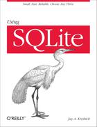
CROSS
                                          JOIN
A CROSS
JOIN matches every row of the first table with every row of the
second table. If the input tables have x
and y columns, respectively, the resulting
table will have x+y columns. If the input
tables have n and m
rows, respectively, the resulting table will have
n·m rows. In mathematics, a CROSS JOIN is known as a
Cartesian product.
The syntax for a CROSS JOIN is quite simple:
SELECT ... FROM t1 CROSS JOIN t2 ...
Figure 5-1 shows
how a CROSS JOIN is
calculated.
Because CROSS
JOINs have the potential to generate extremely
large tables, care must be taken to only use them when
appropriate.
INNER
                                          JOIN
An INNER
JOIN is very similar to a CROSS
JOIN, but it has a built-in condition that is
used to limit the number of rows in the resulting table. The
conditional is normally used to pair up or match rows from the
two source tables. An INNER
JOIN without any type of conditional expression
(or one that always evaluates to true) will result in a CROSS JOIN. If the input tables
have x and y columns,
respectively, the resulting table will have no more than
x+y columns (in some cases, it can
have fewer). If the input tables have n and
m rows, respectively, the resulting
table can have anywhere from zero to n·m
rows, depending on the condition. An INNER JOIN is the most common type of join, and
is the default type of join. This makes the INNER keyword optional.
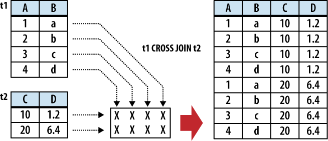
There are three primary ways to specify the
conditional. The first is with an ON expression. This provides a simple
expression that is evaluated for each potential row. Only those
rows that evaluate to true are actually joined. A JOIN...ON looks like
this:
SELECT ... FROM t1 JOIN t2 ON conditional_expression ...An example of this is shown in Figure 5-2.
If the input tables have
C and D columns,
respectively, a JOIN...ON
will always result in C+D columns.
The conditional expression can be used to
test for anything, but the most common type of expression tests
for equality between similar columns in both tables. For
example, in a business employee database, there is likely to be
an employee table that
contains (among other things) a name column and an eid column (employee ID number). Any other
table that needs to associate rows to a specific employee will
also have an eid column that
acts as a pointer or reference to the correct employee. This
relationship makes it very common to have queries with ON expressions similar
to:
SELECT ... FROM employee JOIN resource ON employee.eid = resource.eid ...
This query will result in an output table
where the rows from the resource table are correctly matched to their
corresponding rows in the employee table.
This JOIN
has two issues. First, that ON condition is a lot to type out for something
so common. Second, the resulting table will have two eid columns, but for any given
row, the values of those two columns will always be identical.
To avoid redundancy and keep the phrasing shorter, inner join
conditions can be declared with a USING expression. This expression specifies a
list of one or more columns:
SELECT ... FROM t1 JOIN t2 USING ( col1 ,... ) ...
Queries from the employee database would now look something like this:
SELECT ... FROM employee JOIN resource USING ( eid ) ...
To appear in a USING condition, the column name must exist in
both tables. For each listed column name, the USING
condition will test for equality between the pairs
of columns. The resulting table will have only one instance of
each listed column.
If this wasn’t concise enough, SQL provides an additional
shortcut. A
NATURAL JOIN is similar to a
JOIN...USING, only it
automatically tests for equality between the values of every
column that exists in both tables:
SELECT ... FROM t1 NATURAL JOIN t2 ...
If the input tables have
x and y columns,
respectively, a JOIN...USING
or a NATURAL JOIN will result
in anywhere from max(x,y) to
x+y columns.
Assuming eid is the only column identifier to appear in
both the employee and
resource table, our
business query becomes extremely simple:
SELECT ... FROM employee NATURAL JOIN resource ...
NATURAL
JOINs are convenient, as they are very concise,
and allow changes to the key structure of various tables without
having to update all of the corresponding queries. They can also
be a tad dangerous unless you follow some discipline in naming
your columns. Because none of the columns are explicitly named,
there is no error checking in the sanity of the join. For
example, if no matching columns are found, the JOIN will automatically (and
without warning) degrade to a CROSS
JOIN, just like any other INNER JOIN. Similarly, if two
columns accidentally end up with the same name, a NATURAL JOIN will automatically
include them in the join condition, if you wanted it or
not.
OUTER JOIN
The OUTER
JOIN is an extension of the INNER
JOIN. The SQL standard defines three types of
OUTER JOINs: LEFT, RIGHT, and FULL. Currently, SQLite only supports the
LEFT OUTER JOIN.
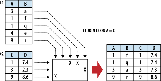
OUTER
JOINs have a conditional that is identical to
INNER JOINs, expressed
using an ON, USING, or NATURAL keyword. The initial
results table is calculated the same way. Once the primary
JOIN is calculated, an
OUTER join will take
any unjoined rows from one or both tables, pad them out with
NULLs, and append them to the resulting table. In the case of a
LEFT OUTER JOIN, this
is done with any unmatched rows from the first table (the table
that appears to the left of the word JOIN).
Figure 5-3 shows
an example of a LEFT OUTER
JOIN.
The result of a LEFT OUTER JOIN will contain at least one
instance of every row from the lefthand table. If the input
tables have x and y
columns, respectively, the resulting table will have no more
than x+y columns (the exact number depends
on which conditional is used). If the input tables have
n and m rows,
respectively, the resulting table can have anywhere from
n to n·m
rows.
Because they include unmatched rows,
OUTER JOINs are often
specifically used to search for unresolved or “dangling”
rows.
Table aliases
Because the JOIN operator combines the columns of different tables into one,
larger table, there may be cases when the resulting working
table has multiple columns with the same name. To avoid
ambiguity, any part of the SELECT statement can qualify any column
reference with a source-table name. However, there are some
cases when this is still not enough. For example, there are some
situations when you need to join a table to itself, resulting in
the working table having two instances of the same source-table.
Not only does this make every column name ambiguous, it makes it
impossible to distinguish them using the source-table name.
Another problem is with subqueries, as they don’t have concrete
source-table names.
To avoid ambiguity within the SELECT statement, any instance
of a source-table, view, or subquery can be assigned an alias.
This is done with the AS
keyword. For example, in the cause of a self-join, we can assign
a unique alias for each instance of the same table:
SELECT ... FROM x AS x1 JOIN x AS x2 ON x1.col1 = x2.col2 ...
Or, in the case of a subquery:
SELECT ... FROM ( SELECT ... ) AS sub ...
Technically, the AS keyword
is optional, and each source-table name can simply
be followed with an
alias name. This can be quite confusing, however, so it is
recommended you use
the AS keyword.
If any of the subquery columns conflict with
a column from a standard source table, you can now use the
sub qualifier as a
table name. For example, sub.col1.
Once a table alias has been assigned, the original source-table name becomes invalid and cannot be used as a column qualifier. You must use the alias instead.
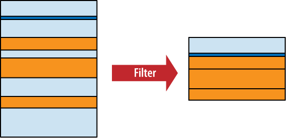
WHERE Clause
The WHERE
clause is used to filter rows from the working table
generated by the FROM clause. It is
very similar to the WHERE clause
found in the UPDATE and DELETE commands. An expression is
provided that is evaluated for each row. Any row that causes the
expression to evaluate to false or NULL is discarded. The resulting
table will have the same number of columns as the original table, but
may have fewer rows. It is not considered an error if the WHERE clause eliminates every row in
the working table. Figure 5-4 shows how the
WHERE clause works.
Some WHERE clauses can get quite
complex, resulting in a long series of AND operators used to join sub-expressions together.
Most filter for a specific row, however, searching for a specific key
value.
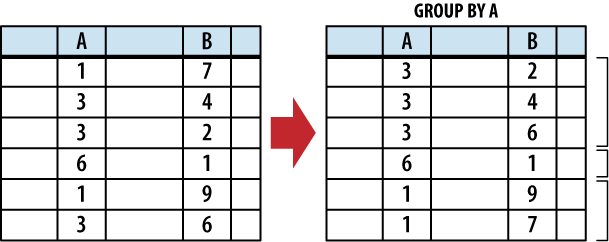
GROUP BY Clause
The GROUP BY
clause is used to collapse, or “flatten,” groups of rows. Groups can be
counted, averaged, or otherwise aggregated together. If you need to
perform any kind of inter-row operation that requires data from more
than one row, chances are you’ll need a GROUP
BY.
The GROUP BY
clause provides a list of grouping expressions and optional
collations. Very often the expressions are simple column references,
but they can be arbitrary expressions. The syntax looks like
this:
GROUP BYgrouping_expression[COLLATEcollation_name] [,...]
The grouping process has two steps. First, the
GROUP
                                    BY
expression list is
used to arrange table rows into different groups. Once the groups are
defined, the SELECT header
(discussed in the next section) defines how those groups are flattened
down into a single row. The resulting table will have one row for each
group.
To split up the working table into groups, the list of expressions is evaluated across each row of the table. All of the rows that produce equivalent values are grouped together. An optional collation can be given with each expression. If the grouping expression involves text values, the collation is used to determine which values are equivalent. For more information on collations, see ORDER BY Clause.
Figure 5-5 shows how
the rows are grouped together with the GROUP
BY clause.
Once grouped together, each collection of rows is
collapsed into a single row. This is typically done using aggregate
functions that are defined in the SELECT heading, which is described in the next
section, on page .
Because it is common to GROUP BY using expressions that are defined in the
SELECT header, it is possible
to simply reference SELECT heading
expressions in the GROUP BY
expression list. If a GROUP BY
expression is given as a literal integer, that number is used as a
column index in the result table defined by the SELECT header. Indexes start at one
with the leftmost column. A GROUP
BY expression can also reference a result column
alias. Result column aliases are explained in the next section.
SELECT Header
The SELECT
header is used to define the format and content of the final result table.
Any column you want to appear in the final results table must be
defined by an expression in the SELECT header. The SELECT heading is the only required step in the
SELECT command
pipeline.
The format of the header is fairly simple, consisting of a list of expressions. Each expression is evaluated in the context of each row, producing the final results table. Very often the expressions are simple column references, but they can be any arbitrary expression involving column references, literal values, or SQL functions. To generate the final query result, the list of expressions is evaluated once for each row in the working table.
Additionally, you can provide a column name
using the AS
keyword:
SELECTexpression[AScolumn_name] [,...]
Don’t confuse the AS keyword used in the SELECT header with the one used in the FROM clause. The SELECT header uses the AS keyword to assign a column name to
one of the output columns, while the FROM clauses uses the AS keyword to assign a source-table alias.
Providing an output column name is optional, but
recommended. The column name assigned to a results table is not
strictly defined unless the user provides an AS column alias. If your application searches for a
specific column name in the query results, be sure to assign a known
name using AS. Assigning a column
name will also allow other parts of the SELECT statement to reference an output column by
name. Steps in the SELECT pipeline
that are processed before the SELECT header, such as the WHERE and GROUP BY
clause, can also reference output columns by name, just as long as the
column expression does not contain an aggregate function.
If there is no working table (no FROM clause), the expression list is
evaluated a single time, producing a single row. This row is then used
as the working table. This is useful to test and evaluate standalone
expressions.
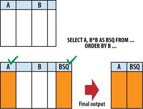
Although the SELECT header appears to filter columns from the
working table, much like the WHERE
clause filters rows, this isn’t exactly correct. All of the columns
from the original working table are still available to clauses that
are processed after the SELECT
header. For example, it is possible to sort the results (via ORDER BY, which is processed after the
SELECT header) using a column
that doesn’t appear in the query output.
It would be more accurate to say that the SELECT header tags specific columns
for output. Not until the whole SELECT pipeline has been processed and the results
are ready to be returned, are the unused columns stripped out. Figure 5-6 illustrates this point.
In addition to the standard expressions, SELECT supports two wildcards. A simple asterisk (*) will cause
every user-defined column from every source table in the FROM clause to be output. You can also
target a specific table (or table alias) using the format table_name.*
Be aware that the SELECT wildcards will not return any automatically
generated ROWID columns. To return
both the ROWID and the user-defined
columns, simply ask for them both:
SELECT ROWID, * FROM table;Wildcards do include any user-defined INTEGER PRIMARY KEY column that have
replaced the standard ROWID column.
See Primary keys for more information about how
ROWID and INTEGER PRIMARY KEY columns
interact.
In addition to determining the columns of the
query result, the SELECT header
determines how row-groups (produced by the GROUP BY clause) are flattened into a single row.
This is done using
aggregate functions. An aggregate function
takes a column expression as input and aggregates, or combines, all of
the column values from the rows of a group and produces a single
output value. Common aggregate functions include count(), min(), max(), and
avg(). Appendix E provides a full list of all the built-in
aggregate
functions.
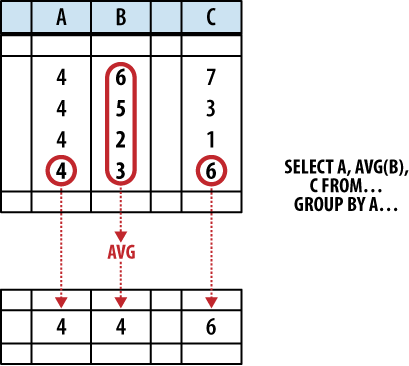
Any column or expression that is not passed
through an aggregate function will assume whatever value was contained
in the last row of the group. However, because SQL tables are
unordered, and because the SELECT
header is processed before the ORDER
BY clause, we don’t really know which row is “last.”
This means the values for any unaggregated output will be taken from
some essentially random row in the group. Figure 5-7 shows how
this works.
In some cases, picking the value from a random row
is not a bad thing. For example, if a SELECT header expression is also used as a GROUP BY expression, then we know that
column has an equivalent value in every row of a group. No matter
which row you choose, you will always get the same value.
Where you can run into trouble is when the
SELECT header uses column
references that were not part of the GROUP
BY clause, nor were they passed through aggregate
functions. In those cases there is no deterministic way to figure out
what the output value will be. To avoid this, when using a GROUP BY clause, SELECT header expressions should only
use column references as aggregate function inputs, or the header
expressions should match those used in the GROUP BY clause.
Here are some examples. In this case all of the expressions are bare column references to help make things clear:
SELECT col1, sum( col2 ) FROM tbl GROUP BY col1; -- well formed
This is a well formed statement. The GROUP BY clause shows that the rows
are being grouped based off the values in col1. That makes it safe for col1 to appear in the SELECT header, since every row in a particular group
will have an equivalent value in col1. The SELECT
header also references col2, but it
is fed into an aggregate function. The aggregate function will take
all of the col2 values from
different rows in the group and produce a logical answer—in this case,
a numerical summation.
The result of this statement will be two columns.
The first column will have one row for each unique value from col1. Each row of the second column
will have the sum of all the values in col2 that are associated with the col1 value listed in the first result
column. More detailed examples can be found at the end of the
chapter.
This next statement is not well formed:
SELECT col1, col2 FROM tbl GROUP BY col1; -- NOT well formed
As before, the rows are grouped based off the
value in col1, which makes it safe
for col1 to appear in the SELECT header. The column col2 appears bare, however, and not as
an aggregate parameter. When this statement is run, the second return
column will contain random values from the original col2 column.
Although every row within a group should have an equivalent value in a
column or expression that was used as a grouping key, that doesn’t
always mean the values are the exact same. If a collation such as
NOCASE was used, different
values (such as 'ABC' and 'abc') are considered equivalent. In
these cases, there is no way to know the specific value that will be
returned from a SELECT header. For
example:
CREATE TABLE tbl ( t ); INSERT INTO tbl VALUES ( 'ABC' ); INSERT INTO tbl VALUES ( 'abc' ); SELECT t FROM tbl GROUP BY t COLLATE NOCASE;
This query will only return one row, but there is no way to know which specific value will be returned.
Finally, if the SELECT header contains an aggregate function, but the
SELECT statement has no
GROUP BY clause, the entire
working table is treated as a single group. Since flattened groups
always return one row, this will cause the query to return only one
row—even if the working table contained no rows.
HAVING Clause
Functionally, the
HAVING clause is identical to the
WHERE clause. The HAVING clause consists of a filter
expression that is evaluated for each row of the working table. Any
row that evaluates to false or NULL is filtered out and removed. The
resulting table will have the same number of columns, but may have
fewer rows.
The main difference between the WHERE clause and the HAVING clause is where they appear in
the SELECT pipeline. The HAVING clause is processed after the
GROUP BY and SELECT clauses, allowing HAVING to filter rows based off the
results of any GROUP BY aggregate.
HAVING clauses can even have
their own aggregates, allowing them to filter on aggregate results
that are not part of the SELECT
header.
HAVING clauses
should only contain filter expressions that depend on the GROUP BY output. All other filtering
should be done in the WHERE
clause.
Both the HAVING
and WHERE clauses can reference
result column names defined in the SELECT header with the AS keyword. The main difference is that the WHERE clause can only reference
expressions that do not contain aggregate functions, while the
HAVING clause can reference
any result column.
DISTINCT Keyword
The DISTINCT
keyword will scan the result set and eliminate any duplicate rows.
This ensures the returned rows constitute a proper set. Only the
columns and values specified in the SELECT header are considered when determining if a
row is a duplicate or not. This is one of the few cases when NULLs are
considered to have “equality,” and will be eliminated.
Because SELECT
DISTINCT must compare every row against every other
row, it is an expensive operation. In a well-designed database, it is
also rarely required. Therefore, its usage is somewhat unusual.
ORDER BY Clause
The ORDER BY
clause is used to sort, or order, the rows of the results table. A
list of one or more sort expressions is provided. The first expression
is used to sort the table. The second expression is used to sort any
equivalent rows from the first sort, and so on. Each expression can be
sorted in ascending or descending order.
The basic format of the ORDER BY clause looks like this:
ORDER BYexpression[COLLATEcollation_name] [ASC|DESC] [,...]
The expression is evaluated for each row. Very
often the expression is a simple column reference, but it can be any
expression. The resulting value is then compared against those values
generated by other rows. If given, the named collation is used to sort
the values. A collation defines a specific sorting order for text
values. The
ASC or DESC keywords can be used to force the sort in an
ascending or descending order. By default, values are sorted in an
ascending order using the default collation.
An ORDER BY
expression can utilize any source column, including those that do not
appear in the query result. Like GROUP
BY, if an ORDER BY
expression consists of a literal integer, it is assumed to be a column
index. Column indexes start on the left with 1, so the phrase ORDER BY 2 will sort the results table
by its second column.
Because SQLite allows different datatypes to be stored in the same column, sorting can get a bit more interesting. When a mixed-type column is sorted, NULLs will be sorted to the top. Next, integer and real values will be mixed together in proper numeric order. The numbers will be followed by text values, with BLOB values at the end. There will be no attempt to convert types. For example, a text value holding a string representation of a number will be sorted in with the other text values, and not with the numeric values.
In the case of numeric values, the natural sort
order is well defined. Text values are sorted by the active collation,
while BLOB values are always sorted using the BINARY collation. SQLite comes with three built-in
collation functions. You can also use the API to define your own
collation functions. The three built-in collations are:
-
BINARY Text values are sorted according to the semantics of the POSIX
memcmp()call. The encoding of a text value is not taken into account, essentially treating it as a large binary string. BLOB values are always sorted with this collation. This is the default collation.-
NOCASE Same as
BINARY, only ASCII uppercase characters are converted to lowercase before the comparison is done. The case-conversion is strictly done on 7-bit ASCII values. The normal SQLite distribution does not support UTF-aware collations.-
RTRIM Same as
BINARY, only trailing (righthand) whitespace is ignored.
While ORDER BY
is extremely useful, it should only be used when it is actually
needed—especially with
very large result tables. Although SQLite can sometimes make use of an
index to calculate the query results in order, in many cases SQLite
must first calculate the entire result set and then sort it, before
rows are returned. In that case, the intermediate results table must
be held in memory or on disk until it is fully computed and can then
be sorted.
Overall, there are plenty of situations where
ORDER BY is justified, if not
required. Just be aware there can be some significant costs involved
in its use, and you shouldn’t get in the habit of tacking it on to
every query “just because.”
LIMIT and OFFSET Clauses
The LIMIT and
OFFSET clauses allow you to extract a specific subset of rows from the
final results table. LIMIT defines
the maximum number of rows that will be returned, while OFFSET defines the number of rows to
skip before returning the first row. If no OFFSET is provided, the LIMIT is applied to the top of the table. If a
negative LIMIT is provided, the
LIMIT is removed and will
return the whole table.
There are three ways to define a LIMIT and OFFSET:
LIMITlimit_countLIMITlimit_countOFFSEToffset_countLIMIToffset_count,limit_count
Caution
Note that if both a limit and offset are given using the third format, the order of the numbers is reversed.
Here are some examples. Notice that the OFFSET value defines how many rows are
skipped, not the position of the first row:
LIMIT 10             -- returns the first 10 rows (rows 1 - 10)
LIMIT 10 OFFSET 3    -- returns rows  4 - 13
LIMIT 3  OFFSET 20   -- returns rows 21 - 23
LIMIT 3, 20          -- returns rows  4 - 23 (different from above!)
Although it is not strictly required, you usually
want to define an ORDER BY if
you’re using a LIMIT. Without an
ORDER BY, there is no
well-defined order to the result, making the limit and offset somewhat
meaningless.